


Highlights
What are the main findings?
- DO is a non-optically active parameter, but it can be indirectly estimated using satellite-derived optical variables. A temporal lag exists between satellite-derived surface optical variables and bottom-water DO response; explicitly accounting for this delay significantly improves the accuracy of bottom DO retrieval.
- The inversion framework successfully reproduced the spatiotemporal variation in bottom-water DO in the Bohai Sea, revealing two main hypoxic zones in summer.
What are the implications of the main findings?
- The delayed response of bottom-water DO to surface bio-optical signals indicates that biogeochemical processes linked to organic matter sinking and oxygen-consuming decomposition in bottom waters influence DO variability.
- The inversion framework reveals the feasibility of monitoring coastal bottom-water hypoxia using multi-source satellite remote sensing, providing a scalable and cost-effective approach to long-term ecological assessment, marine management, and early warning for hypoxia events.
Abstract
Seasonal hypoxia in bottom waters of the Bohai Sea poses an escalating threat to marine ecosystems, yet monitoring it via satellite remote sensing continues to be challenging due to the inaccessibility of bottom layers. However, surface bio-optical signals do not instantaneously reflect variation in bottom-water dissolved oxygen (DO); instead, a distinct temporal lag exists between surface biological activity and its influence on bottom DO. Leveraging this insight, an inversion framework was established, integrating multi-source remote sensing data with decision tree-based machine learning models to estimate bottom-water DO concentration. We evaluated multiple lag intervals for satellite-derived bio-optical variables and adopted a 14-day lag as representative of the delayed impact of surface processes on bottom DO. An optimized feature set selected via a genetic algorithm (GA) was used to train the XGBoost model, which achieved high predictive performance (R2 = 0.86, RMSE = 0.79 mg/L, MAPE = 8.89%). Interpretability analysis identified the sea surface temperature as the dominant driver of bottom-water DO variation in the Bohai Sea. The framework successfully reproduced the spatiotemporal variability in bottom DO from 2022 to 2024 in the Bohai Sea and captured the locations of summer hypoxic zones. Further analysis demonstrated that incorporating physically based bottom-layer variables substantially enhances model accuracy (R2 = 0.89, RMSE = 0.68 mg/L, MAPE = 7.85%), underscoring their critical role in regulating bottom-water DO concentrations. Building on the established inversion framework and integrating extended in situ and satellite observations, we reconstruct the long-term temporal distribution of bottom DO in the Bohai Sea from 2014 to 2025, revealing the considerable potential of satellite data for monitoring bottom-water DO conditions in coastal seas.
1. Introduction
Dissolved oxygen (DO) is a fundamental indicator of aquatic ecosystem health. Its concentration is influenced by both natural factors (e.g., water temperature, salinity, freshwater input, and eutrophication processes) and human activities (e.g., agricultural fertilization, urbanization, and industrial wastewater discharge). DO levels below 2 mg/L are generally defined as hypoxia, while values under 4 mg/L are considered low-oxygen conditions. These conditions can persist for days to months, often resulting in the mortality or displacement of aerobic organisms, thereby disrupting ecosystem structure and function. Globally, hypoxic zones have doubled in number roughly every ten years since the 1960s [1]. A global oceanic oxygen decline of 1–7% is projected by the end of the next century [2]. As such, systematic monitoring of DO in the water column is essential for ecological risk prevention and the sustainable management of marine resources.
In recent years, summertime bottom hypoxia in the Bohai Sea has attracted significant interest among the research community [3,4,5]. Water stratification in the Bohai Sea typically begins to develop in April and reaches its peak intensity in August [6]. This pronounced stratification strongly suppresses vertical mixing between surface and bottom waters, thereby impeding the downward transport of oxygen-rich surface water to the bottom [7]. Concurrently, the prevailing anticyclonic circulation during summer facilitates the lateral advection of hypoxic waters, further modulating the spatial distribution of hypoxic zones [8]. Moreover, strong wind events can partially alleviate or even suppress hypoxia development by enhancing vertical mixing [9,10]. Intensified anthropogenic activities have exacerbated a suite of recurrent environmental issues, including eutrophication and harmful algal blooms [11]. Driven by substantial terrestrial nutrient inputs, primary productivity in the Bohai Sea is markedly enhanced during summer. Pronounced phytoplankton blooms are frequently observed in regions such as northeast of the Yellow River estuary [12]. Upon senescence, these phytoplankton generate organic particulate matter that sinks to the seabed, where microbial degradation consumes DO [13].
In situ data collection through shipboard surveys and fixed-station observations is costly and often fails to provide adequate spatial and temporal resolution for effective water quality monitoring. The rapid advancement of satellite remote sensing has enabled full-area coverage, regular data acquisition, and dynamic environmental monitoring, making it a valuable tool for water quality assessment. Optically active parameters such as total suspended matter, colored dissolved organic matter (CDOM), and chlorophyll-a (Chl-a) exhibit distinct absorption and scattering characteristics within specific spectral ranges, allowing their estimation through reflectance analysis across various remote sensing spectral bands [14,15,16]. Unlike optically active constituents, parameters such as total nitrogen and DO lack strong absorption or scattering signatures and therefore cannot be directly inferred from spectral reflectance. However, they often show some correlation with optically active components in aquatic systems [17,18,19]. Recent studies have made notable progress in establishing machine learning-based mapping models between DO and multi-spectral remote sensing reflectance (Rrs) [20,21,22]. However, these studies have largely been confined to DO in surface waters. In fact, hypoxic events of ecological concern typically occur in bottom waters, yet there are currently few systematic efforts to retrieve or predict bottom-water DO using remote sensing. Li et al. [23] estimated the spatiotemporal variation in hypoxic zones in the Gulf of Mexico using 14 surface-derived variables from MODIS, although the model’s accuracy was limited. Zhang et al. [24] predicted bottom-water DO distributions over the East China Sea shelf by integrating satellite-derived variables with reanalysis-based sea surface fields; however, the incorporation of DO data derived from numerical simulations to compensate for sparse in situ measurements may have introduced additional uncertainties. Although current methods are restricted by challenges related to accuracy and data scarcity, ongoing advancements in satellite remote sensing capabilities, data fusion techniques, and machine learning algorithms are progressively improving the reliability of bottom-water DO estimation.
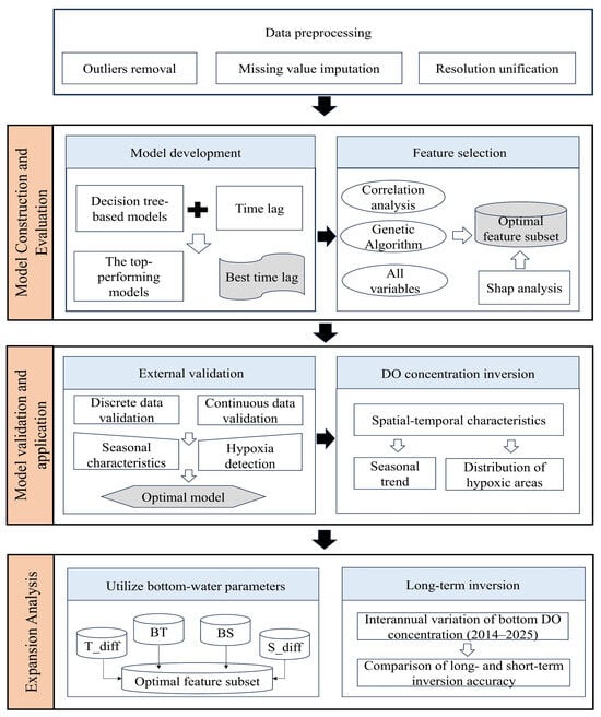
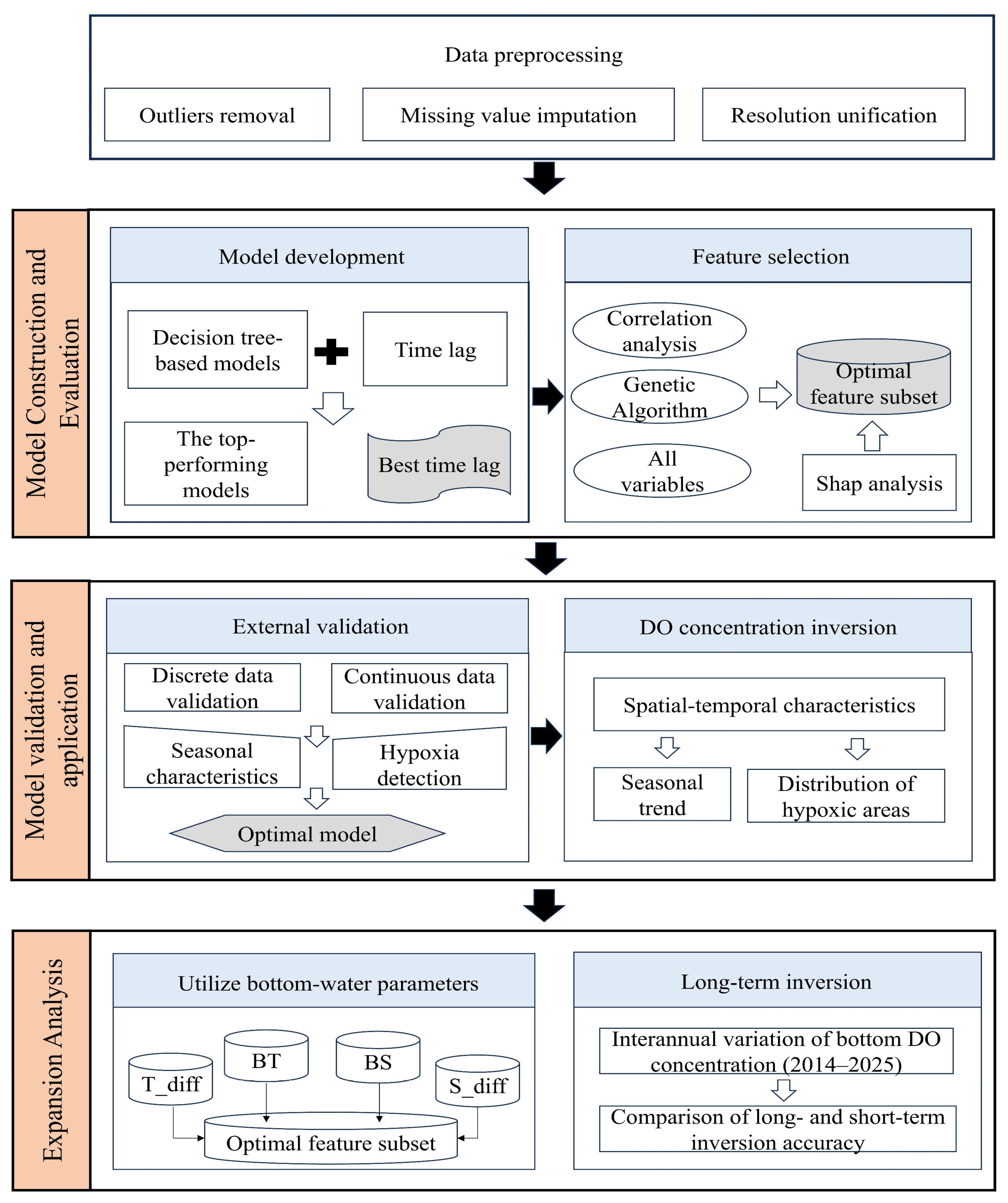
Given that summer hypoxia in the Bohai Sea results from the combined effects of physical and biogeochemical processes, we select explanatory variables that capture this coupled physical–biological framework. In this study, we develop a machine learning model to estimate bottom-water DO concentration in the Bohai Sea using satellite remote sensing data. The overall technical approach is illustrated in Figure 1. Accounting for time lags between surface optical signals and bottom biogeochemical responses, the model reproduces the spatiotemporal distribution of bottom DO from 2022 to 2024. The model performance improves when bottom-layer variables such as bottom temperature and stratification strength are included as predictors. By establishing spectral consistency between GOCI and GOCI-II, we apply the trained model to generate bottom DO estimates spanning the period from 2014 to 2025.
Figure 1.
The technical approach taken in this research.
2. Materials and Methods
2.1. Study Region
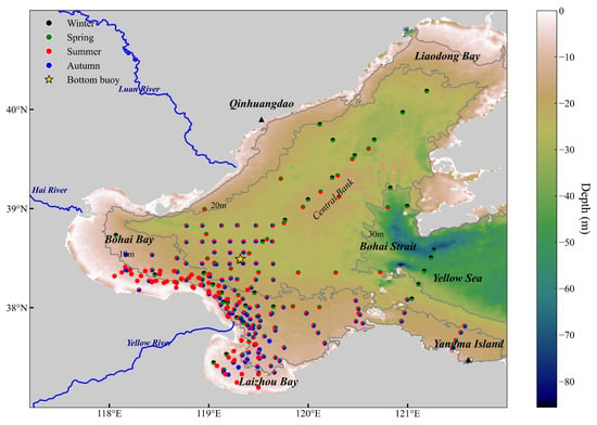
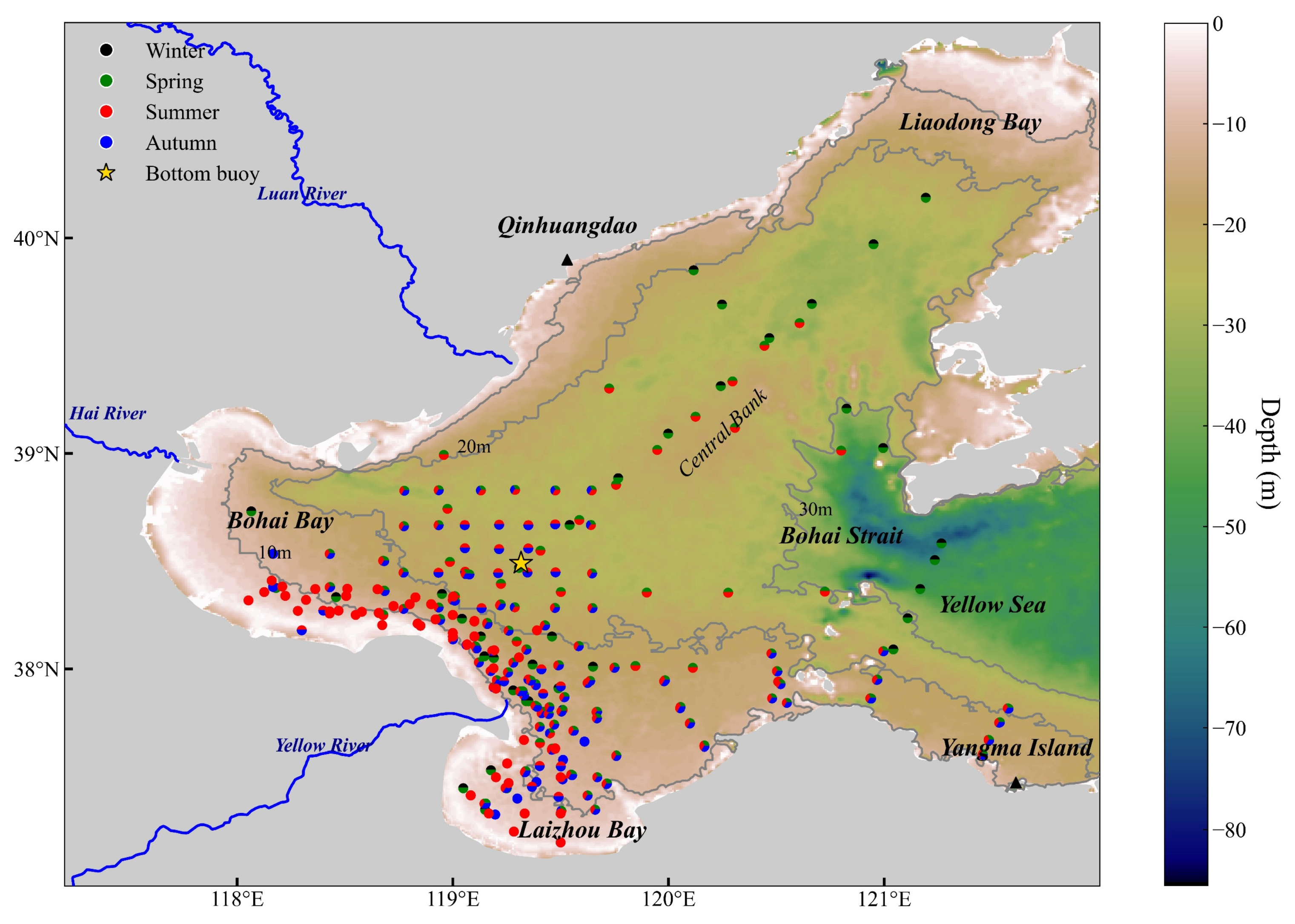
The Bohai Sea has been selected as the study area (Figure 2). As a semi-enclosed inland sea in China with an average depth of 18 m, it is surrounded by land on three sides and connected to the North Yellow Sea solely through the Bohai Strait. This enclosed configuration, comparable to that of the Baltic Sea and Chesapeake Bay, facilitates the development and persistence of seasonal oxygen depletion in certain regions [25]. Within the central Bohai Sea lies a shallow area (Central Bank), and hypoxic conditions frequently occur during summer in the depressions to its northwest and southwest [8,10,26].
Figure 2.
DO sampling stations across different seasons from 2022 to 2024 in the Bohai Sea. Seasonal samplings are indicated in green (spring), red (summer), blue (autumn), and black (winter). Most stations were resampled across different seasons. The star marks the location of the bottom buoy.
2.2. Data Sources
This study includes multi-source data (Table 1). A total of 592 in situ bottom-water DO observations were collected from 217 survey stations in the Bohai Sea between 2022 and 2024 (Figure 2 and Figure S1), with most measurements taken during spring, summer, and autumn. Additionally, we used DO concentration data collected from a bottom buoy in the central Bohai Sea between 20 June and 25 August 2023 (Figure 2). The monitoring system was equipped with an EXO2 multiparameter water quality sonde (YSI Inc., Yellow Springs, OH, USA) integrating a dissolved oxygen sensor. These data were recorded at half-hourly intervals and were employed for the application and validation of the models. Based on the national water quality standard (GB 3097-1997 [27]), seawater with DO levels below 4 mg/L is classified as severely polluted and meets Class IV criteria. Accordingly, hypoxia is defined as DO concentrations at or below 4 mg/L in this study.
Table 1.
Description of data sources.
This study primarily utilizes remote sensing observations from the Geostationary Ocean Color Imager (GOCI) and its upgraded version, GOCI-II, both operating from geostationary orbit. GOCI, mounted on South Korea’s Communication, Ocean and Meteorological Satellite (COMS), acquired eight scenes per day and measured radiance in eight spectral bands spanning 412–865 nm. It served as a key input dataset for long-term bottom-water DO concentration inversion, as reported in Section 4.2.
Although GOCI ceased operations in March 2021, it was succeeded by GOCI-II, launched aboard the GEO-KOMPSAT-2B satellite on 18 February 2020. As the next-generation geostationary ocean color sensor, GOCI-II provides improved spatial resolution (250 m) and maintains a high temporal sampling frequency (10 observations per day). In addition to the 12-band Rrs data (see Table 1), six Level-2 GOCI-II products were selected for analysis: Chl-a, CDOM, primary production (PP), low sea surface salinity (LSSS), sea surface current (SSC), and total suspended sediment (TSS). SSC_speed (m/s) and SSC_direction (°) are directly provided by the GOCI-II Level-2 SSC product.
Sea surface temperature (SST) data were obtained from the Multiscale Ultrahigh Resolution (MUR) SST product, a Group for High Resolution Sea Surface Temperature Level 4 analysis. The MUR SST is provided globally at a spatial resolution of 0.01°and integrates observations from multiple satellite sensors, including AMSR-E, AMSR2, MODIS, WindSat, and AVHRR, along with in situ measurements. The data were accessed via https://search.earthdata.nasa.gov/, accessed on 27 August 2025.
The Hybrid Coordinate Ocean Model (HYCOM) is a global ocean general circulation model that combines the advantages of isopycnic, terrain-following, and z-level coordinates to better resolve complex ocean dynamics. HYCOM data have been previously applied for DO-related studies in the Bohai Sea [8,10]. Bottom-water environmental variables, specifically bottom temperature (BT) and bottom salinity (BS), were obtained from HYCOM and used in the analysis presented in Section 4.1.
All multi-source datasets, originally varying in spatial resolution and coverage, were resampled onto a uniform 1 × 1 km grid using linear interpolation. This processing framework is primarily based on GOCI-II ocean color observations and MUR sea surface temperature data and is designed to investigate how surface-water environmental parameters influence the spatiotemporal patterns of bottom-water DO concentrations in the Bohai Sea. The contributions of additional datasets, including historical GOCI records and HYCOM-simulated bottom conditions, will be evaluated in subsequent analyses and discussion.
2.3. Methods
2.3.1. Machine Learning Algorithms
To identify suitable approaches to bottom-water DO inversion, several mainstream machine learning algorithms are selected and compared in this study. An emphasis is placed on decision tree-based models, which are well suited for capturing nonlinear relationships and feature interactions, and have demonstrated strong adaptability and generalization in DO inversion and prediction tasks [24,28,29].
Among these, eXtreme Gradient Boosting (XGB), Light Gradient Boosting Machine (LGB), and Categorical Boosting (CB) represent widely used implementations of the gradient boosting decision tree algorithm, offering strong nonlinear modeling capabilities and effective identification of feature importance. Each employs distinct algorithmic designs to enhance performance and efficiency. XGB introduces an explicit regularization term in its objective function to penalize model complexity, thereby improving generalization. LGB accelerates training through a leaf-wise tree growth strategy and histogram-based feature binning, which is particularly advantageous for large datasets. CB addresses prediction bias by implementing ordered boosting, a permutation-driven approach that uses independent samples to compute gradients and natively supports categorical features without preprocessing. These characteristics make them well suited for modeling complex, nonlinear relationships in environmental data such as bottom-water DO.
Meanwhile, random forest (RF) and extremely randomized trees (ERT) are employed as representative Bagging-based methods. These models generate diverse ensembles of decision trees and aggregate their outputs, enhancing robustness against overfitting and noise. The structures and underlying principles of the five models are detailed in Text S1. All models were implemented in Python 3.11. Specifically, XGB, CB, and LGB were implemented using their respective dedicated libraries (xgboost, catboost, and lightgbm), while RF and ERT were implemented using the scikit-learn library. Detailed hyperparameter configurations are provided in Table S1 [30,31,32,33,34].
All models were trained and evaluated using a consistent preprocessing framework, which included data standardization, an 8:2 training-to-testing split, and hyperparameter tuning via cross-validation and grid search. This ensured methodological consistency and reliable comparison among model performances.
2.3.2. Time Lag Effect
DO concentrations of bottom water at a given time are influenced by sea surface environmental conditions from preceding periods, necessitating the inclusion of temporal lag effects in modeling efforts [35,36]. Numerical simulations have demonstrated a lag of 1–8 weeks between surface diatom production and bottom-water hypoxia in the Yangtze River estuary [37]. Similarly, studies in Chesapeake Bay have shown that winter and spring wind conditions can affect summer hypoxia through alterations to circulation patterns [38]. A time lag has also been observed between satellite-derived surface parameters and in situ bottom-water DO concentrations. For example, Li et al. [23] identified lag periods of 0–5 days and 16–19 days between surface-water phenomena, such as algal blooms, and the onset of bottom hypoxia using ocean color variables. In light of these findings, the present study assumes that remote sensing explanatory variables from within 1 month before DO sampling may influence bottom-water DO concentrations at the time of observation. Due to the limitations of optical remote sensing data, such as reduced availability caused by cloud cover and atmospheric interference [39], the 1-month lag period is divided into five discrete time intervals: 0 (no lag), 7, 14, 21, and 28 days. For each interval, the corresponding remote sensing variables are extracted to evaluate the influence of time-lagged environmental conditions on bottom-water DO. For GOCI and GOCI-II-derived variables (e.g., Rrs, Chla), the matching observation time was constrained to within ±8 h of the target lag time. For SST, BT, and BS, no time lag was applied, and the temporal matching window was set to ±2 h.
2.3.3. Model Performance Evaluation
To assess the predictive performance of the machine learning models on the test set, three statistical metrics were employed: the coefficient of determination (R2), the root mean square error (RMSE), and the mean absolute percentage error (MAPE). The R2 metric reflects the proportion of variance in the observed values that can be explained by the predicted values; values closer to 1 indicate a better model fit. RMSE measures the average magnitude of prediction errors in absolute terms, with smaller values representing higher predictive accuracy. MAPE quantifies the relative error between predicted and observed values, where lower percentages indicate stronger model generalization and stability. The corresponding formulas for these metrics are given in Equations (1)–(3):
where n represents the total number of DO observation samples, and yi, , and denote the i-th actual observed DO value, the corresponding predicted DO value, and the mean of all observed DO values, respectively.
2.3.4. Identification of Key Input Variables
To enhance model interpretability and reduce potential redundancy among input variables, a feature subset selection procedure was implemented following the identification of the optimal time lag. Given that hypoxia arises from coupled physical–biological processes, individual predictors are likely to exhibit varying degrees of association with bottom-water DO. A genetic algorithm (GA) coupled with XGB was employed to search for the optimal combination of predictors. The GA used the negative RMSE on the validation set as the fitness function, thereby favoring subsets that maximize predictive accuracy. Each individual in the GA population represented a binary mask indicating the inclusion (1) or exclusion (0) of each variable. The search was conducted over 20 generations with a population size of 50, using tournament selection, two-point crossover, and bit-flip mutation.
2.3.5. Explanatory Ability of the Model
In today’s complex, data-driven decision-making environments, the interpretability of artificial intelligence models has become increasingly critical. The emergence of eXplainable artificial intelligence (XAI) has addressed this need through improvements to the transparency and comprehensibility of model behavior, which is essential for fostering user trust, diagnosing errors, and refining model performance [40]. Among various XAI techniques, SHapley Additive exPlanations (SHAP) has been widely adopted as a state-of-the-art method [41]. Rooted in Shapley values from cooperative game theory, SHAP offers a unified framework to quantify the contribution of each input feature to a model’s output by fairly distributing the prediction influence across all possible feature combinations, expressed through Equation (4):
where ϕi represents the SHAP value of the i-th feature; S denotes any subset of features that excludes feature i; N denotes the complete collection of input features; and fx(S) represent the model output when only the features in subset S ⊆ N are active. The operator “∪” denotes set union and “!” denotes the factorial operator. The magnitude of ϕi quantifies the influence of feature i on the prediction; i.e., a larger absolute value indicates a greater influence. A positive SHAP value suggests that the feature increases the prediction, while a negative value implies a suppressive effect. SHAP values near zero indicate minimal impact on the current prediction. This formulation evaluates each feature’s importance in the context of all possible feature combinations, thereby enabling detailed, instance-level interpretability of model outputs.
3. Results
3.1. Model Performance Comparison
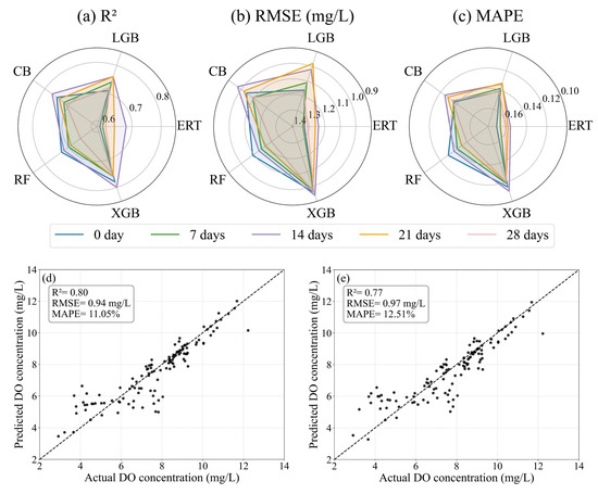
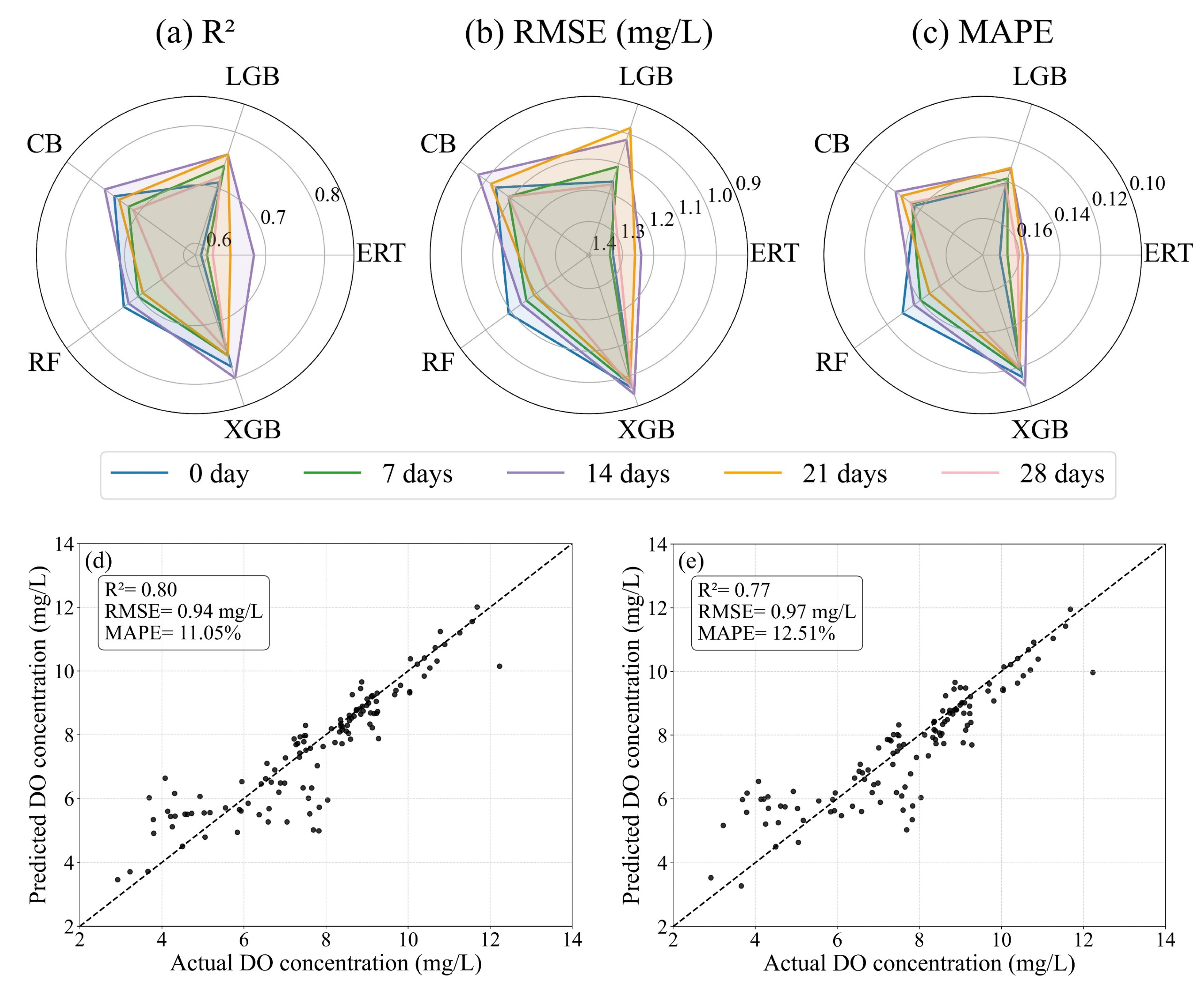
For each time lag, all GOCI-II variables, together with SST, were used as inputs to train the five tree-based models. Across all lag windows, XGB, LGB, CB, and RF generally achieved R2 values above 0.7 (Figure 3a), indicating that these decision tree-based models show a reasonable capacity to capture patterns in DO concentration. Most models achieved peak performance with a 14-day time lag. Specifically, XGB (R2 = 0.80, RMSE = 0.94 mg/L, MAPE = 11.05%) and CB (R2 = 0.77, RMSE = 0.97 mg/L, MAPE = 12.51%) achieved the best performance among all models (Figure 3d,e). Although RF performed best among all models with a 0-day lag, its performance was still inferior to that of XGB and CB. In contrast, ERT demonstrated the weakest predictive performance across the time lags, likely due to its fully randomized splitting mechanism, which selects split values randomly from the feature range. This approach may reduce accuracy when modeling complex or nonlinear relationships. The other four models optimize split points by minimizing error or loss functions at each node, which enhances predictive accuracy. Therefore, XGB and CB with a 14-day lag were selected for further analysis in this study.
Figure 3.
(a–c) Model performance on the test set under different time lags (averaged over 100 training repetitions). (d,e) Performance of XGB and CB with a 14-day time lag. (d) XGB model, (e) CB model.
3.2. Comparative Evaluation of Feature Subsets
With the optimal time lag fixed at 14 days, we constructed three distinct input feature subsets, denoted as Subset 1, Subset 2, and Subset 3, to evaluate the trade-offs between model complexity and predictive performance (Table 2). Subset 1 was based on Pearson correlation analysis between each predictor and in situ bottom DO concentrations (Figure S2a). Only variables with absolute correlation coefficients exceeding 0.25 were retained, resulting in six features. For instance, SST exhibited the strongest correlation with DO (r = −0.88), followed by PP (r = −0.35). Subset 2 was identified through the GA that used negative RMSE on the validation set as the fitness criterion. Variable selection frequencies (Figure S2b) quantify this evolutionary process, with higher values indicating a stronger contribution to minimizing validation error. SST emerged as the most critical predictor, appearing in all 20 generations. Ultimately, this process yielded an optimal combination of nine variables. Subset 3 included all 20 available variables derived from GOCI-II data and MUR SST.
Table 2.
Features in each subset.
Each subset was used to train both XGB and CB models under identical hyperparameter configurations and data splits. Their predictive performances on the internal test set are summarized in Table 3, which shows that models trained on Subset 2 achieve the best balance of accuracy and parsimony, consistently outperforming those based on Subset 1 and Subset 3. Therefore, Subset 2 is adopted as the input feature set for subsequent modeling in Section 3.3, Section 3.4, and Section 3.5.
Table 3.
Predictive performance of XGB and CB models using different feature subsets.
3.3. Interpretability of the Model
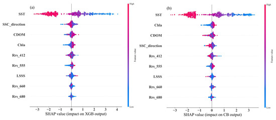
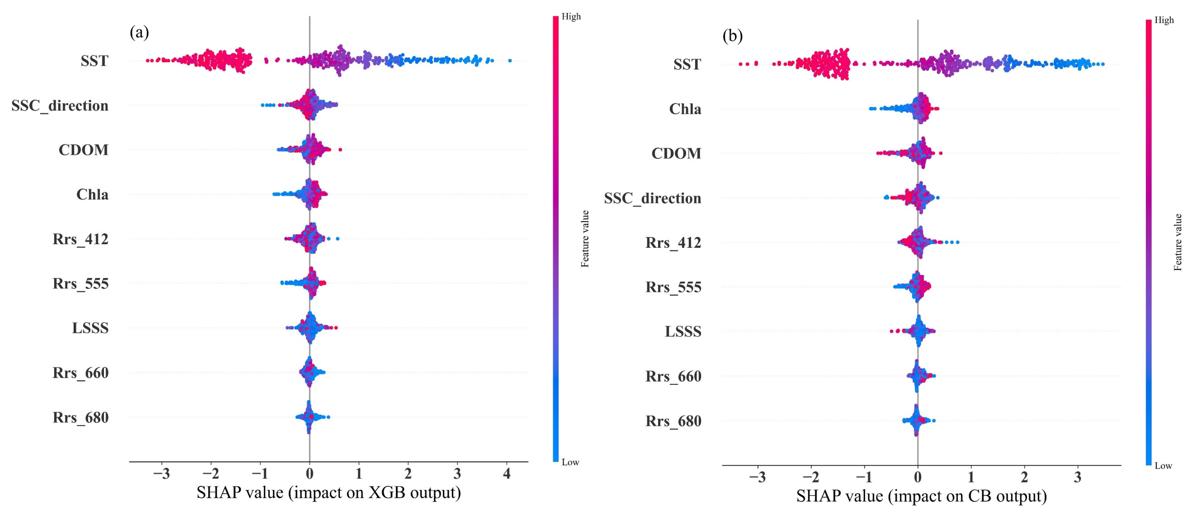
SHAP interpretability analysis reveals the nonlinear contributions of the eight GA-selected variables to bottom DO predictions in both the XGB and CB models (Figure 4). SST emerges as the most influential predictor in both models, with higher SST values consistently associated with negative SHAP contributions, indicating that elevated SST tends to reduce bottom DO concentrations. This effect is primarily attributed to enhanced stratification, which suppresses vertical mixing and restricts the downward transport of oxygen-rich surface waters.
Figure 4.
SHAP values of explanatory variables under a 14-day time lag: (a) XGB model. (b) CB model.
Among the spectral reflectance bands, Rrs_412 and Rrs_555 (blue-green wavelengths) exhibit substantially higher importance than the red bands (Rrs_660 and Rrs_680) in both models. The stronger influence of the blue-green bands reflects their sensitivity to surface organic matter dynamics [42], with the impact on bottom DO being delayed due to the time required for particulate material to settle and undergo microbial decomposition in deeper layers. This delayed response is explicitly accounted for in our time-lagged modeling framework.
Furthermore, Chl-a shows consistently positive SHAP contributions across both models, suggesting that, within the adopted 14-day time lag window, it primarily functions as a proxy for recent photosynthetic oxygen production, and the associated oxygenation signal has not yet been offset by subsequent oxygen consumption from organic matter remineralization. Concurrently, SSC_direction also demonstrates discernible influence in both models, underscoring the significant role of oceanic dynamical processes in shaping the spatial distribution of DO.
3.4. External Validation Against Independent in Situ Measurements
To further assess the applicability and reliability of the XGB and CB models for bottom-water DO concentration inversion, two independent validation experiments were conducted.
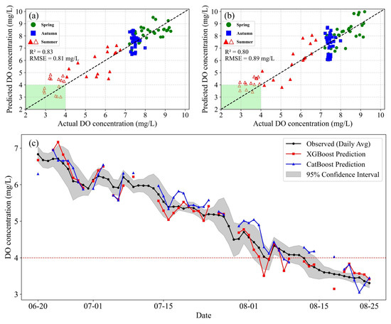
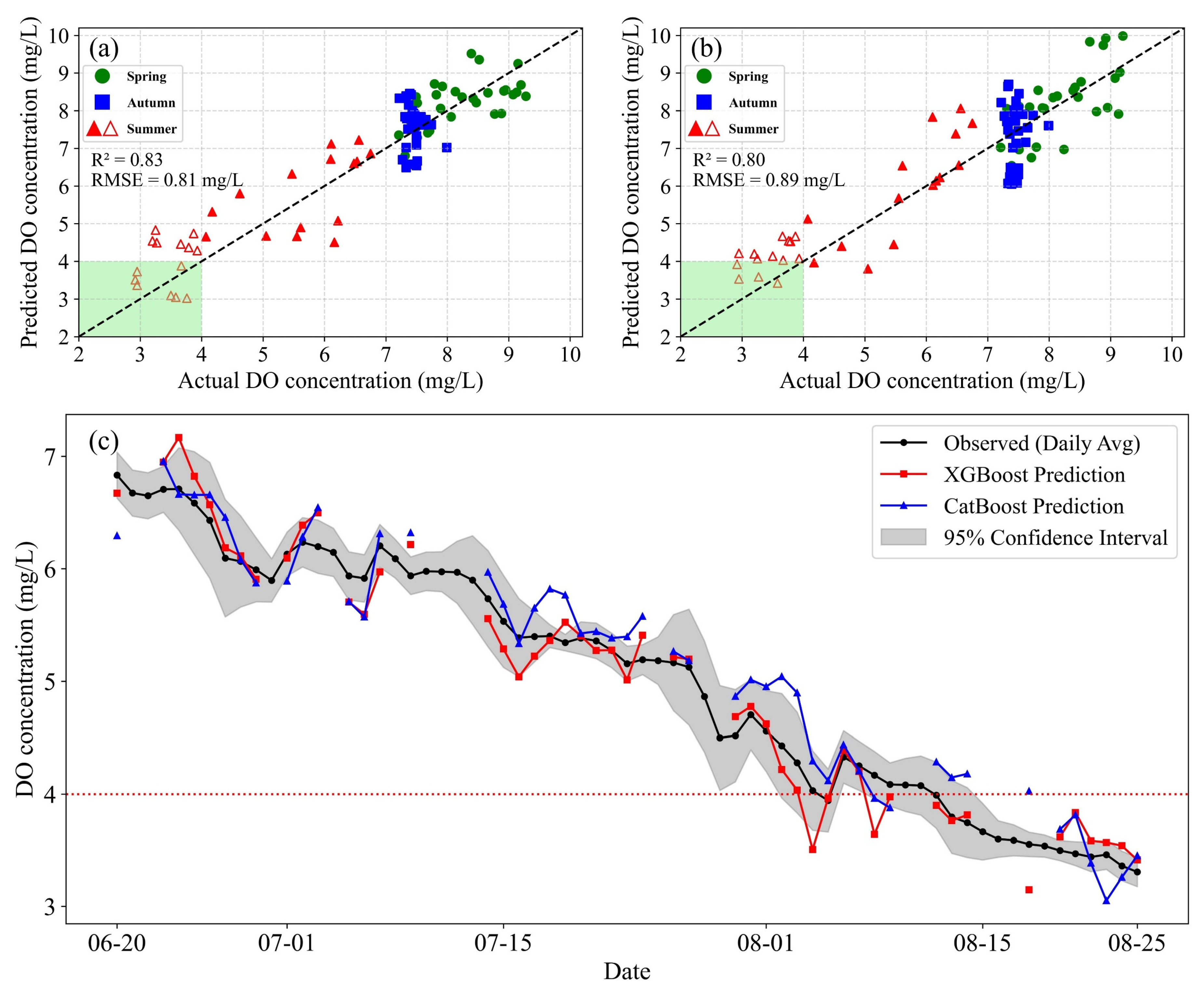
Seasonal hypoxia in the central Bohai Sea has recently been documented, with Guo et al. [9] reporting a pronounced hypoxic event in 2022 based on field observations. The first experiment in this study utilizes in situ DO data collected from 29 sampling stations during the same cruise, covering three seasons: 28 May–2 June (spring), 29 August–4 September (summer), and 8–15 November (autumn). During the summer survey, hypoxic conditions (DO ≤ 4 mg/L) were observed at 14 stations (Figure S3). This well-documented hypoxia event provides a robust observational basis for evaluating the performance of models in detecting hypoxic conditions. A comparison between the inversion results generated using the XGB and CB models and the corresponding field measurements showed that both models successfully captured the seasonal distribution patterns of DO (Figure 5a,b). Among them, the XGB model exhibited greater sensitivity in identifying hypoxic stations (Figure 5a). Specifically, Figure S4 presents the results from independent validation experiment 1, showing that across Spring, Summer, and Autumn, the predicted mean DO concentrations and their corresponding distribution ranges for both models were generally consistent with the in situ measurements. Additionally, compared to the preliminary modeling experiments that used all input variables to determine the optimal time lag (Figure 3d,e), both models driven by Subset 2 show improved overall performance, including in the low oxygen range, where DO ≤ 4 mg/L, further confirming the effectiveness of the selected feature subset. Furthermore, in situ bottom DO concentrations from the 29 independent validation stations were overlaid onto the inversion maps of selected days for each season (Figure S5). The colors of the overlaid dots broadly match the surrounding background fields, indicating a reasonable spatial consistency between the observed and inverted DO concentrations.
Figure 5.
(a,b) Independent validation experiment 1. (a) XGB model, (b) CB model. Solid symbols indicate non-hypoxic stations; hollow symbols indicate hypoxic stations. The green shaded area marks the stations correctly identified as hypoxic by the model. The autumn validation points appear vertically stacked due to the limited range of observed DO concentrations, although the model still predicts a wider spread of values. (c) Independent validation experiment 2. Comparison of predicted DO concentrations from the XGB and CB models with bottom-recorded DO concentrations, when satellite data are available. The red dotted line represents the hypoxia concentration threshold.
The second experiment is based on time-series data collected from a bottom buoy deployed in the central Bohai Sea in 2023 (Figure 2). DO concentrations recorded by the bottom buoy were processed into daily averaged time series for analysis. The inversion results derived from this dataset show that both the XGB and CB models accurately capture the seasonal trend of DO concentration during summer (Figure 5c). Predicted values generally fall within the confidence interval, indicating a stable and reliable model performance over time. Under hypoxic conditions, the XGB model demonstrates notably superior predictive accuracy.
The results of the two experiments collectively demonstrate that both XGB and CB models are effective in inverting bottom-water DO concentrations from remote sensing data, exhibiting high accuracy and strong practical applicability. Among the two, the XGB model consistently outperforms in identifying hypoxic conditions across both spatial and temporal dimensions. Accordingly, XGB is selected as the benchmark model for bottom-water DO inversion in subsequent analyses.
3.5. The Spatial–Temporal Variation in the DO Concentration
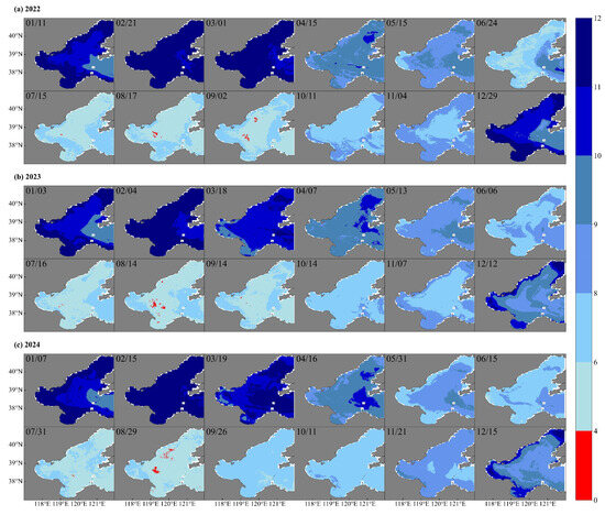
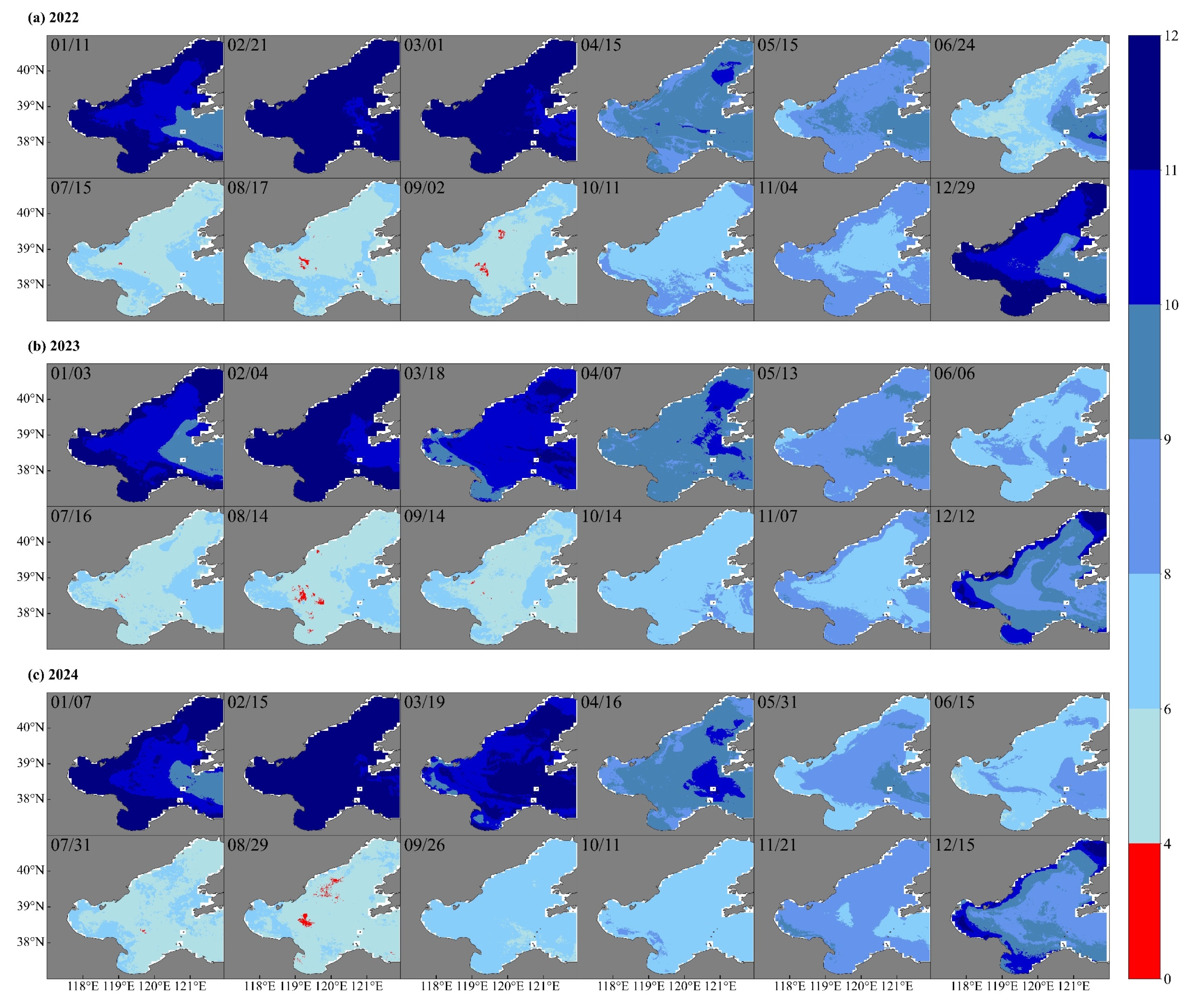
Using the established optimal inversion model, which is the XGB model configured with the optimal feature subset selected using GA, bottom-water DO concentrations in the Bohai Sea were successfully retrieved for the period of 2022–2024 (Figure 6). To reduce the influence of adverse meteorological conditions, such as cloud cover, that can interfere with electromagnetic wave propagation and degrade remote sensing data quality [43,44], the day with the most favorable weather conditions in each month was selected for inversion. This approach was designed to produce outputs that most accurately reflect actual environmental conditions. The resulting 3-year dataset reveals pronounced spatiotemporal variability in bottom-water DO concentrations across the Bohai Sea.
Figure 6.
Spatiotemporal distribution of inverted DO concentrations from 2022 to 2024.
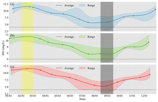
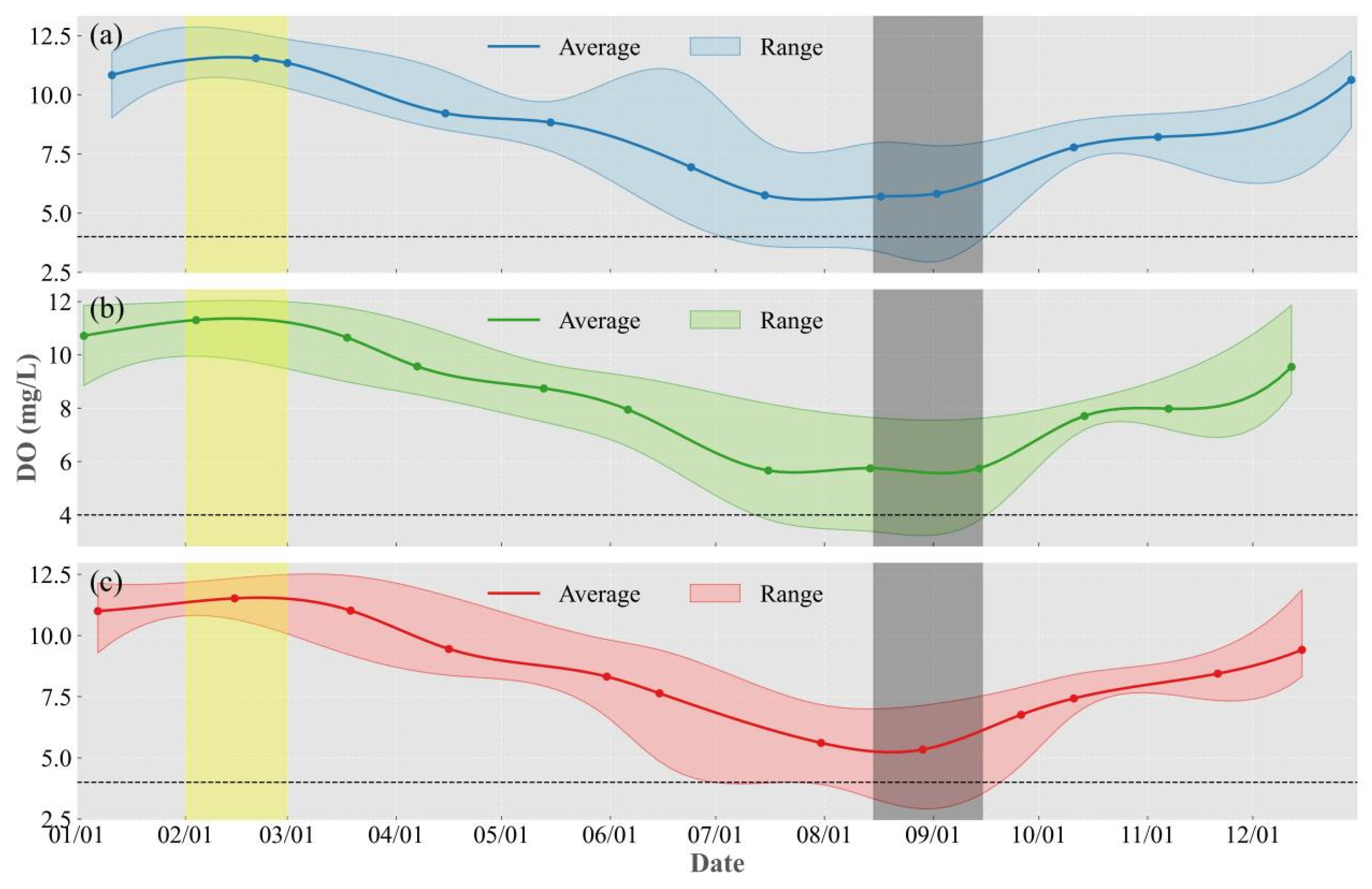
The inversion results reveal a distinct annual cycle in bottom-water DO concentrations in the Bohai Sea (Figure 7). DO levels peak between February and March, decline steadily thereafter, reach their lowest levels in late August, and begin to recover in September. This seasonal pattern aligns with previous numerical simulation findings [8]. In 2022, bottom-water DO concentrations peaked at approximately 12.5 mg/L in early February, followed by a gradual decline to around 2.9 mg/L by late August. From September onward, concentrations increased and nearly returned to initial levels by the end of the year. A similar trend was observed in 2023, although the peak was slightly lower at approximately 12.0 mg/L, and the minimum was slightly higher at about 3.4 mg/L. In 2024, the DO cycle remained largely consistent with the preceding years, reaching a peak of around 12.4 mg/L and a minimum of 2.9 mg/L. This three-year record highlights a consistent seasonal pattern: bottom-water DO concentrations are relatively high in winter and spring, moderate in autumn, and lowest in summer. During winter, bottom-water DO concentrations reach their annual peak, with an average of 10.72 mg/L. This increase is supported by relatively strong wind conditions associated with the East Asian monsoon [45,46], which enhance vertical mixing and facilitate DO exchange throughout the water column. Nutrient levels also rise during this period [47], establishing a basis for spring phytoplankton growth. In spring, the average bottom-water DO concentration remains relatively high, at approximately 9.68 mg/L. The lowest DO concentrations occur in summer, with the bottom-water average decreasing to 6.26 mg/L and hypoxic conditions arising in some regions. Ocean warming during this period intensifies stratification, while lower wind speeds and weakened turbulent kinetic energy limit vertical mixing [48], reducing oxygen transfer to the bottom layers. Simultaneously, elevated temperatures accelerate the decomposition and mineralization of organic matter, further increasing oxygen demand in the bottom waters [9,49]. By autumn, the average bottom-water DO concentration rises to 7.32 mg/L. This recovery is attributed to declining SST and increasing wind speeds, which enhance vertical mixing and contribute to the mitigation of hypoxic conditions.
Figure 7.
(a–c) Mean and extreme bottom DO concentrations for 2022–2024; from top to bottom, panels correspond to 2022, 2023, and 2024. Each point represents the spatially averaged bottom DO concentration across the entire Bohai Sea derived from the inversion model on the specific date corresponding to the DO concentration spatial mapping shown in Figure 6. Yellow and gray bands indicate peak and minimum DO periods, respectively.
Based on the inversion results during the study period (2022–2024), two primary seasonal hypoxic zones were identified, both located within the dual cold-water masses in the central Bohai Sea (Figure 6). These zones are located in the deep water surrounding the Central Bank, where strong summer stratification impedes vertical exchange of dissolved oxygen between surface and bottom waters, creating stable conditions conducive to the development and persistence of hypoxia. This spatial distribution is consistent with previous observations derived from field measurements [50,51] and numerical simulations, which also reported persistent hypoxia in the double-core cold-water region from 2014 to 2019 [10]. By mid-July, hypoxia had already developed in the southern cold-water region of the Bohai Sea. The hypoxic extent in this region continued to expand in August, persisted through mid-September, and disappeared by the end of September. In the northern cold-water region, a hypoxic zone developed with a similar temporal pattern, lasting until late September. Smaller and shorter-lived hypoxic zones were also detected in Laizhou Bay. These were less persistent due to the bay’s shallow depth and limited water volume and the influence of tidal action, wind-driven mixing, and coastal currents, which enhance vertical water exchange and prevent sustained oxygen depletion. Additionally, seasonal hypoxia was identified in nearshore waters east of Yangma Island in both 2022 and 2024. In this area, hypoxic conditions emerged by mid-August and largely dissipated by early September, in agreement with observations reported by Zheng et al. [52].
4. Discussion
4.1. Modeling Gains from Incorporating Bottom-Water Parameters
While surface-derived remote sensing variables provide useful proxies for processes influencing bottom DO, they lack direct information on the physical state of the bottom layer. To address this limitation, we augmented the original subset of nine variables selected by the GA with four HYCOM-derived bottom-layer parameters: BT, BS, and the differences between surface and bottom temperature (T_diff) and salinity (S_diff). To verify the reasonableness of these HYCOM-simulated variables, we compared them against the in situ bottom measurements collected at the 29 stations in independent validation experiment 1 (Figure S6).
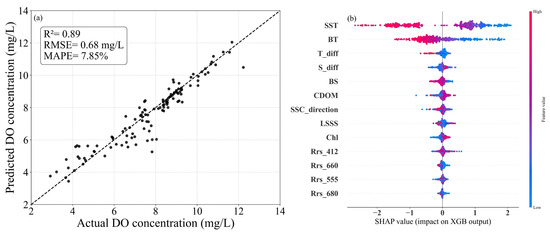
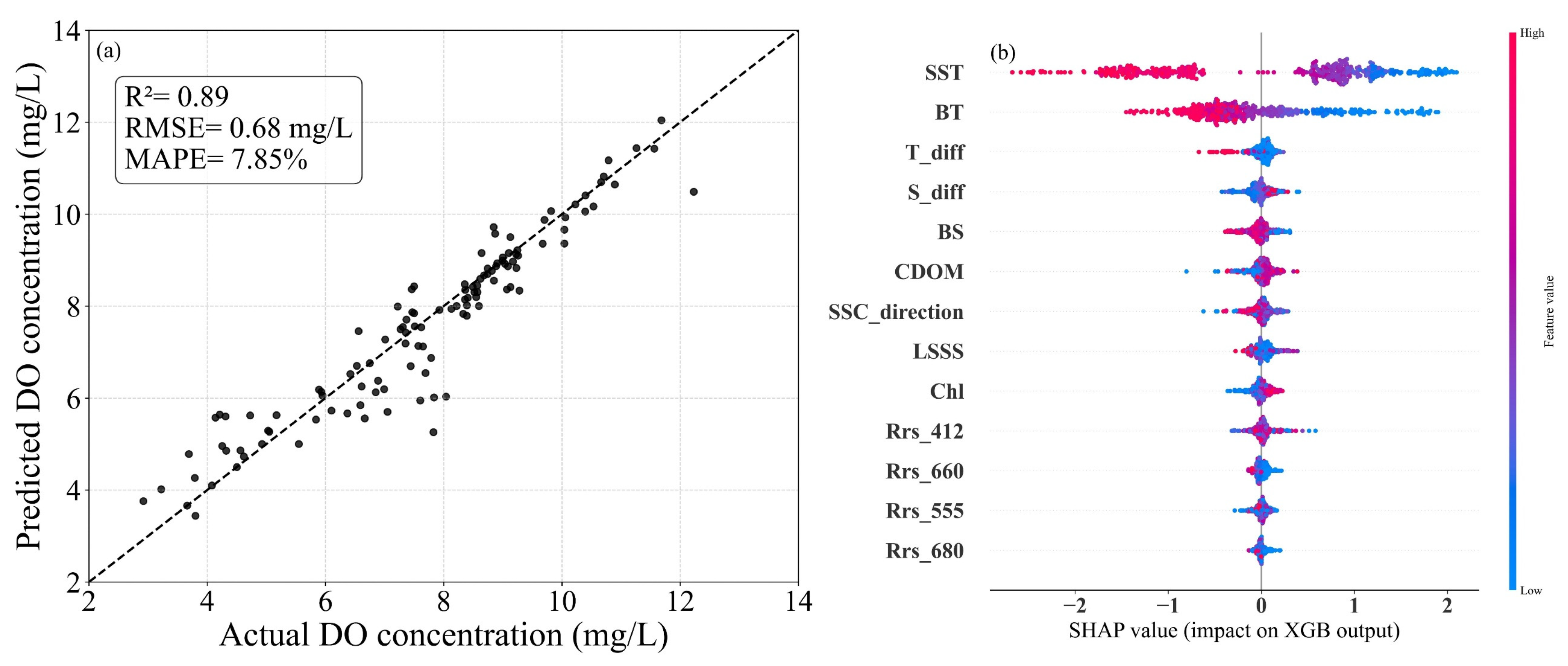
The XGB model was then retrained using this expanded input set under identical hyperparameter and validation settings. Model performance improved markedly after incorporating these bottom-layer descriptors: R2 increased from 0.86 to 0.89, RMSE decreased from 0.79 mg/L to 0.68 mg/L, and MAPE dropped from 8.89% to 7.85% (Figure 8a). This improvement highlights the critical role of explicit bottom-condition information in accurately capturing DO concentrations, particularly in coastal systems such as the Bohai Sea where vertical stratification is pronounced in summer.
Figure 8.
Under the condition of incorporating bottom-water body parameters: (a) the performance of the XGB model; (b) SHAP values of explanatory variables.
SHAP analysis of the augmented model (Figure 8b) revealed that BT ranks as the second most important predictor after SST. This is physically interpretable: BT directly controls the solubility of oxygen in bottom waters and also modulates microbial metabolic rates, thereby indirectly influencing oxygen consumption [53,54]. In contrast, S_diff was consistently assigned low importance by both models relative to T_diff, suggesting that salinity-driven stratification plays a comparatively minor role in regulating bottom DO, which aligns with prior studies [55].
4.2. Feasibility of Long-Term Inversion Using Combined GOCI and GOCI-II Data
To enable long-term monitoring of bottom-water DO concentrations in the Bohai Sea, we extended the inversion framework beyond the 2022–2024 period by incorporating an expanded in situ dataset comprising 1528 DO observations collected between 2014 and 2025 (including the original 592 samples) (Figure S7). Although the optimal variable set derived from GOCI-II data during 2022–2024 yielded the best performance, some of its input variables are not available during the earlier GOCI. To ensure consistency across the full time series, we used only the eight spectral bands common to both GOCI (2011–2021) and GOCI-II (2020–present), Rrs at 412, 443, 490, 555, 660, 680, 745, and 865 nm, together with MUR SST. Prior to model training, cross-calibration was performed between GOCI and GOCI-II Rrs data in the overlapping bands, following the approach described by Qin et al. [56] to minimize inter-sensor biases. The long-term XGB model was trained on this consistent input set to support the long-term analysis of bottom DO.
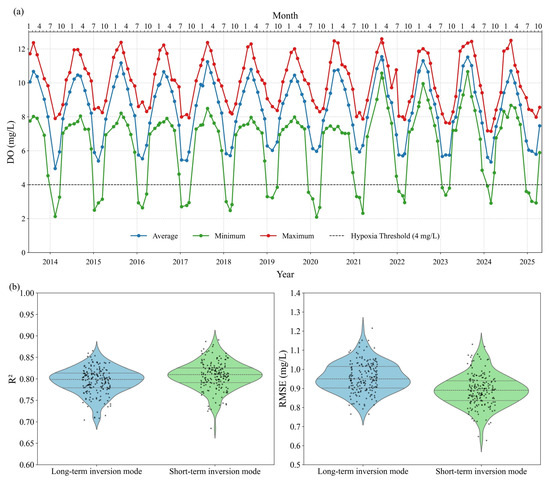
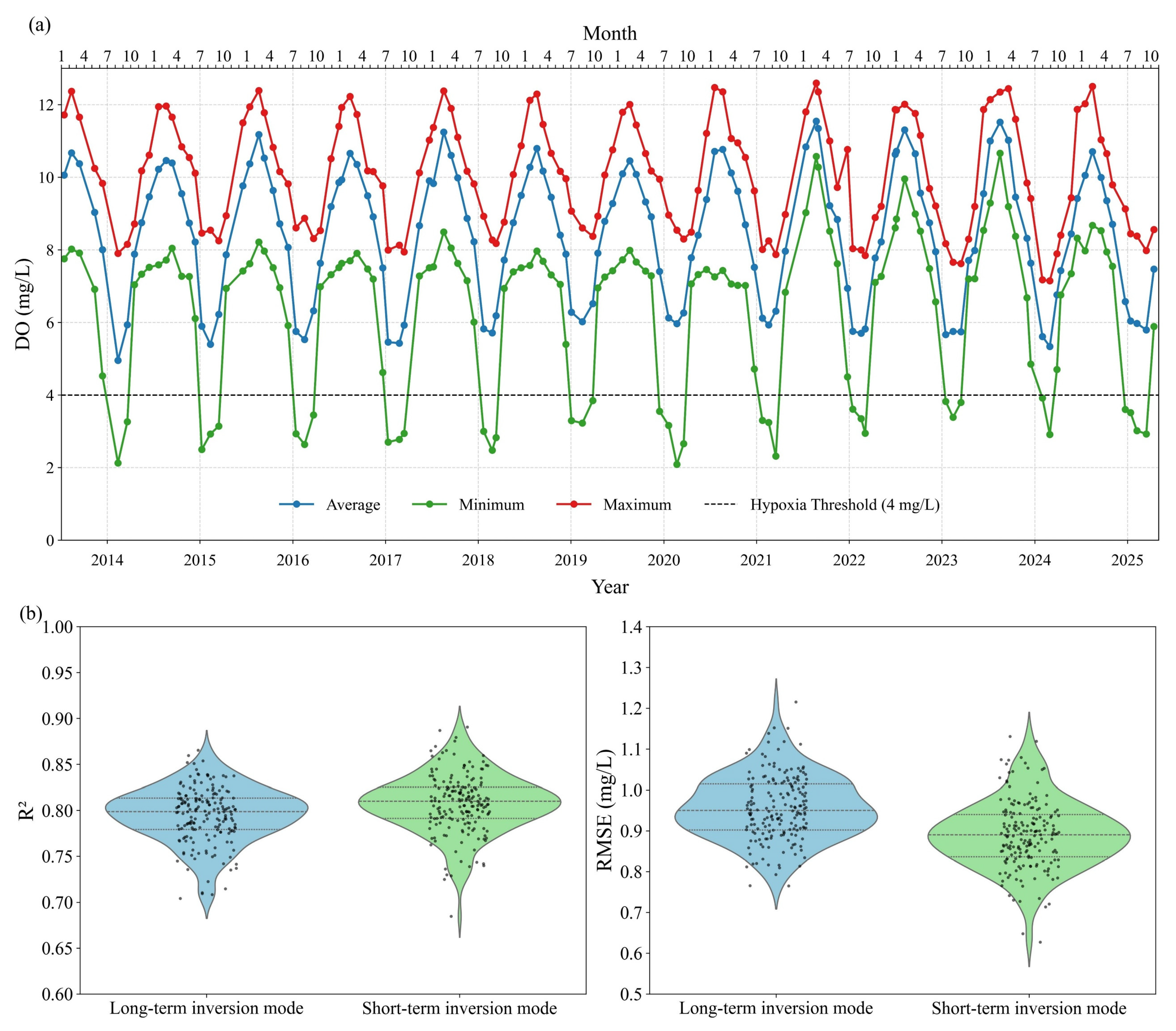
The resulting 12-year DO time series, though not derived from continuous daily inversion, reveals a highly consistent seasonal cycle in agreement with the patterns described in Section 3.5 (Figure 9a). Analysis of annual minimum DO concentrations during July–September shows that values frequently fall below the hypoxia threshold of 4 mg/L, with many years recording minima of 2–3 mg/L or even lower in localized regions. Examination of the full record does not indicate a systematic worsening trend in summer hypoxia over the 2014–2025 period. However, the seasonal occurrence of hypoxia highlights the need for sustained monitoring to assess ecological risks in the Bohai Sea.
Figure 9.
(a) The interannual variation (from 2014 to 2025) of the bottom DO concentration in the Bohai Sea obtained through inversion using the XGB model (each point corresponds to the optimal inversion date within the month). (b) Between 2022 and 2024, 180 dates were selected and used to perform long-term and short-term inversions with the XGB model. The left panel shows the distribution of R2 values for each sample in the test set under both inversion modes, while the right panel shows the corresponding distribution of RMSE values.
To evaluate the consistency between the short-term (2022–2024) and long-term (2014–2025) inversion frameworks, we systematically compared the performance of the XGB model in terms of R2 and RMSE on the test set, using 180 representative dates from their overlapping period. The results show that both frameworks demonstrate good predictive performance: the median R2 values for both short-term and long-term inversions are around 0.8, indicating that each approach effectively captures the spatiotemporal variability of bottom DO concentrations (Figure 9b). Meanwhile, the median RMSE of the long-term inversion exceeds that of the short-term inversion by about 0.06 mg/L—a difference that could be attributed to the lower spatial resolution of GOCI relative to GOCI-II, as well as reduced consistency between the two sensors in the blue spectral bands [57], which somewhat limits retrieval accuracy. Figure S8 presents a spatial comparison of bottom DO concentrations derived from the long-term and short-term inversions during periods of frequent hypoxia. These results confirm the feasibility of cross-sensor (GOCI and GOCI-II) inversion for bottom DO, a conclusion further supported by prior studies on the retrieval of other aquatic parameters [58]. Short-term inversion provides higher accuracy and is well suited for analyzing recent DO dynamics, while long-term inversion enables the assessment of bottom DO over a broader temporal scale, albeit with slightly lower accuracy. These two frameworks are thus complementary and jointly enable both high-quality monitoring and long-term trend assessment of bottom DO in the Bohai Sea.
5. Conclusions
In this study, we developed and evaluated five decision tree-based machine learning models for bottom-water DO retrieval in the Bohai Sea, based on multi-source remote sensing data from 2022 to 2024. Central to our approach is the explicit consideration of the temporal lag in bottom-water DO response to surface bio-optical signals. Based on an optimal feature set selected via the GA, the XGB model achieved optimal performance with a 14-day temporal lag window, yielding satisfactory predictive accuracy on the internal test set (R2 = 0.86, RMSE = 0.79 mg/L, MAPE = 8.89%) and exhibiting good generalization on independent validation datasets. According to SHAP-based interpretability analysis, SST emerged as the dominant factor influencing bottom DO concentration. Spatiotemporal analysis of the retrieved DO concentrations captured pronounced seasonal variation and identified two seasonal hypoxic zones in the central Bohai Sea.
To assess the extensibility of the approach, bottom-layer temperature and salinity were incorporated as additional predictors, which substantially improved the model accuracy (R2 = 0.89, RMSE = 0.68 mg/L, MAPE = 6.75%), demonstrating the critical value of including bottom physical parameters for enhancing DO retrieval capability. Furthermore, by leveraging the spectral continuity between GOCI and GOCI-II, a preliminary framework was developed to support consistent long-term reconstruction of bottom DO concentrations in the Bohai Sea, offering a viable pathway toward monitoring changes in coastal hypoxia.
This study has several limitations. Firstly, the determination of the optimal time lag was based on evaluating a few discrete, isolated lag intervals. This approach may overlook more complex or continuous lag–response relationships between surface conditions and bottom DO. Future work could employ more sophisticated methods, such as cross-wavelet analysis, to provide a more comprehensive and continuous characterization of these temporal lags across different time scales. Secondly, this study was focused on reconstructing the seasonal cycle of bottom DO; we did not analyze interannual variability in hypoxic event dynamics such as onset, duration, or spatial extent, nor did we link these features to year-specific oceanographic conditions. Future work should investigate these aspects to better understand the drivers of interannual differences in hypoxia. Thirdly, wind plays a critical role in driving vertical mixing and modulating bottom oxygen replenishment, particularly during storm events, so future work could consider incorporating high-resolution wind-forcing data such as those from ERA5. Integrating such dynamic drivers is key to enabling short-term early warning of hypoxic events.
Supplementary Materials
The following supporting information can be downloaded at: https://www.mdpi.com/article/10.3390/rs18050838/s1, Figure S1: The distribution of sampling stations over the past three years. Figure S2: (a) Correlation between each variable and DO. (b) Feature selection frequency of GA. Figure S3: The sampling data range used in the first independent verification experiment. Figure S4: In the independent verification test 1, the mean values and distribution ranges of the DO concentration as observed in situ and predicted by the two models. Figure S5: Spatial validation of inverted DO concentrations by overlaying in situ measurements from the 29 stations onto the DO inversion map for a selected day within the corresponding spring, summer, and autumn sampling periods. Figure S6: During repeated observations at 29 stations in the central Bohai Sea, comparisons were made between in situ measurements and model outputs for both bottom temperature and salinity. Figure S7: (a) Monthly distribution of DO concentrations from field sampling sites during 2014–2025, shown as violin plots with medians highlighted in red; (b) spatial distribution of the same sampling sites. Figure S8: Spatial distribution of bottom-water DO concentration in the Bohai Sea during periods when hypoxia commonly occurs, as estimated using the XGB model under long-term and short-term inversion schemes, along with the difference between two inversion results. Each row corresponds to a specific date. Table S1: Hyperparameter configurations of each model. Text S1: Introduction to the model algorithm [30,31,32,33,34].
Author Contributions
Conceptualization, S.L.; Methodology, T.L. and Y.J.; Validation, T.L.; Investigation, J.G., D.J., C.H. and H.T.; Resources, D.J.; Data Curation, J.G., Y.J., D.J., C.H. and H.T.; Writing—Original Draft, T.L.; Writing—Review and Editing, J.G. and S.L.; Visualization, T.L.; Supervision, J.G. and S.L.; Project Administration, J.G.; Funding Acquisition, J.G. All authors have read and agreed to the published version of the manuscript.
Funding
This work was supported in part by the National Natural Science Foundation of China under Grant U2106211 and Grant 42076197.
Data Availability Statement
The data presented in this study are available upon request from the corresponding author.
Acknowledgments
Some of the data used in this study were provided by the Data Center of the Yantai Institute of Coastal Zone Research, Chinese Academy of Sciences. Additional data and samples were collected aboard R/V Lanhai101 during the open research cruises NORC2025-01, NORC2024-01, and NORC2023-01, supported by the NSFC Shiptime Sharing Project (Nos. 42449901, 42349901, 42249901).
Conflicts of Interest
The authors declare no conflicts of interest.
Abbreviations
The following abbreviations are used in this manuscript:
| DO | dissolved oxygen |
| CDOM | colored dissolved organic matter |
| Chl-a | chlorophyll-a |
| GOCI | Geostationary Ocean Color Imager |
| GOCI-II | Geostationary Ocean Color Imager II |
| Rrs | remote sensing reflectance |
| PP | primary production |
| LSSS | low sea surface salinity |
| SSC | sea surface current |
| TSS | total suspended sediment |
| SST | sea surface temperature |
| MUR | Multiscale Ultrahigh Resolution |
| HYCOM | Hybrid Coordinate Ocean Model |
| BT | bottom temperature |
| BS | bottom salinity |
| XGB | eXtreme Gradient Boosting |
| LGB | Light Gradient Boosting Machine |
| CB | Categorical Boosting |
| RF | random forest |
| ERT | extremely randomized tree |
| GA | genetic algorithm |
| XAI | eXplainable artificial intelligence |
| SHAP | SHapley Additive exPlanations |
| T_diff | the differences between surface and bottom temperature |
| S_diff | the differences between surface and bottom salinity |
References
- Diaz, R.J.; Rosenberg, R. Spreading Dead Zones and Consequences for Marine Ecosystems. Science 2008, 321, 926–929. [Google Scholar] [CrossRef] [Scilit]
- Keeling, R.F.; Körtzinger, A.; Gruber, N. Ocean Deoxygenation in a Warming World. Annu. Rev. Mar. Sci. 2010, 2, 199–229. [Google Scholar] [CrossRef] [Scilit]
- Zhang, W.; Zhang, H.; Song, G.; Zhao, L.; Wei, H. Physical and biogeochemical processes in controlling the seasonal variation of dissolved oxygen in the Bohai and Yellow Seas. Front. Mar. Sci. 2025, 12, 1600636. [Google Scholar] [CrossRef] [Scilit]
- Wei, H.; Zhao, L.; Zhang, H.; Lu, Y.; Yang, W.; Song, G. Summer hypoxia in Bohai Sea caused by changes in phytoplankton community. Anthr. Coasts 2021, 4, 77–86. [Google Scholar] [CrossRef] [Scilit]
- Wu, M.; Sun, J.; Shi, L.; Guo, J.; Morovati, K.; Lin, B.; Li, Y. Vertical water renewal and dissolved oxygen depletion in a semi-enclosed Sea. J. Hydrol. 2024, 637, 131369. [Google Scholar] [CrossRef] [Scilit]
- Zhai, W.; Zhao, H.; Zheng, N.; Xu, Y. Coastal acidification in summer bottom oxygen-depleted waters in northwestern–northern Bohai Sea from June to August in 2011. Chin. Sci. Bull. 2012, 57, 753–758. [Google Scholar] [CrossRef] [Scilit]
- Guo, J.; Ji, D.; Zheng, X.; Li, Y.; Tang, H.; Hou, C. Stratification in central Bohai Sea and how it has shaped hypoxic events in summer. Acta Oceanol. Sin. 2024, 43, 93–104. [Google Scholar] [CrossRef] [Scilit]
- Zhang, H.; Wei, H.; Zhao, L.; Zhao, H.; Guo, S.; Zheng, N. Seasonal evolution and controlling factors of bottom oxygen depletion in the Bohai Sea. Mar. Pollut. Bull. 2022, 174, 113199. [Google Scholar] [CrossRef] [Scilit]
- Guo, J.; Jin, Y.; Liu, S.; Li, T.; Ji, D.; Hou, C.; Tang, H. Investigation of the causes and mechanisms of hypoxia in the central Bohai Sea in the summer of 2022. Mar. Pollut. Bull. 2024, 206, 116710. [Google Scholar] [CrossRef] [Scilit]
- Wang, H.; Zhang, H.; Wei, H.; Zuo, H. Temporal variations of the two oxygen depleted zones in the Bohai Sea. Front. Mar. Sci. 2023, 10, 1247579. [Google Scholar] [CrossRef] [Scilit]
- Song, N.-Q.; Wang, N.; Lu, Y.; Zhang, J.-R. Temporal and spatial characteristics of harmful algal blooms in the Bohai Sea during 1952–2014. Cont. Shelf Res. 2016, 122, 77–84. [Google Scholar] [CrossRef] [Scilit]
- Cao, J.; Wang, Y.; Liu, X.; Zhou, Y.; Liu, Y.; Yuan, Y. Analysis on the causes of hypoxia in the bottom of the central Bohai Sea in summer 2020. Mar. Environ. Sci. 2023, 42, 254–261. [Google Scholar] [CrossRef]
- Li, Z.; Wei, H.; Zhang, H.; Zhao, H.; Zheng, N.; Song, G. The interannual difference in summer bottom oxygen deficiency in Bohai Sea. Oceanol. Limnol. Sin. 2021, 52, 601–613. [Google Scholar] [CrossRef]
- Qiu, Z.; Liu, D.; Yan, N.; Yang, C.; Chen, P.; Zhang, C.; Duan, H. Improving the observations of suspended sediment concentrations in rivers from Landsat to Sentinel-2 imagery. Int. J. Appl. Earth Obs. Geoinf. 2024, 134, 104209. [Google Scholar] [CrossRef] [Scilit]
- Ling, Z.; Sun, D.; Wang, S.; Qiu, Z.; Huan, Y.; Mao, Z.; He, Y. Remote sensing estimation of colored dissolved organic matter (CDOM) from GOCI measurements in the Bohai Sea and Yellow Sea. Environ. Sci. Pollut. Res. 2020, 27, 6872–6885. [Google Scholar] [CrossRef] [Scilit]
- Harvey, E.T.; Kratzer, S.; Philipson, P. Satellite-based water quality monitoring for improved spatial and temporal retrieval of chlorophyll-a in coastal waters. Remote Sens. Environ. 2015, 158, 417–430. [Google Scholar] [CrossRef] [Scilit]
- Chen, L.; Liu, L.; Liu, S.; Shi, Z.; Shi, C. The Application of Remote Sensing Technology in Inland Water Quality Monitoring and Water Environment Science: Recent Progress and Perspectives. Remote Sens. 2025, 17, 667. [Google Scholar] [CrossRef] [Scilit]
- Ding, L.; Qi, C.; Li, G.; Zhang, W. TP Concentration Inversion and Pollution Sources in Nanyi Lake Based on Landsat 8 Data and InVEST Model. Sustainability 2023, 15, 9678. [Google Scholar] [CrossRef] [Scilit]
- Tan, Z.; Ren, J.; Li, S.; Li, W.; Zhang, R.; Sun, T. Inversion of Nutrient Concentrations Using Machine Learning and Influencing Factors in Minjiang River. Water 2023, 15, 1398. [Google Scholar] [CrossRef] [Scilit]
- Kim, Y.H.; Son, S.; Kim, H.-C.; Kim, B.; Park, Y.-G.; Nam, J.; Ryu, J. Application of satellite remote sensing in monitoring dissolved oxygen variabilities: A case study for coastal waters in Korea. Environ. Int. 2020, 134, 105301. [Google Scholar] [CrossRef] [Scilit]
- Dong, L.; Wang, D.; Song, L.; Gong, F.; Chen, S.; Huang, J.; He, X. Monitoring Dissolved Oxygen Concentrations in the Coastal Waters of Zhejiang Using Landsat-8/9 Imagery. Remote Sens. 2024, 16, 1951. [Google Scholar] [CrossRef] [Scilit]
- Batur, E.; Maktav, D. Assessment of Surface Water Quality by Using Satellite Images Fusion Based on PCA Method in the Lake Gala, Turkey. IEEE Trans. Geosci. Remote Sens. 2019, 57, 2983–2989. [Google Scholar] [CrossRef]
- Li, Y.; Robinson, S.V.J.; Nguyen, L.H.; Liu, J. Satellite prediction of coastal hypoxia in the northern Gulf of Mexico. Remote Sens. Environ. 2023, 284, 113346. [Google Scholar] [CrossRef] [Scilit]
- Zhang, C.; Meng, Q.; Ma, X.; Liu, A.; Zhou, F. Modeling Bottom Dissolved Oxygen on the East China Sea Shelf Using Interpretable Machine Learning. J. Mar. Sci. Eng. 2025, 13, 359. [Google Scholar] [CrossRef] [Scilit]
- Zhang, W.; Pan, S.; Yu, L.; Zhang, H.; Chen, F.; Song, G.; Hu, J.; Wei, Q.; Zhao, H.; Chen, J.; et al. Dissolved oxygen depletion in Chinese coastal waters. Water Res. 2025, 272, 123004. [Google Scholar] [CrossRef] [Scilit]
- Zhou, F.; Huang, D.; Xue, H.; Xuan, J.; Yan, T.; Ni, X.; Zeng, D.; Li, J. Circulations associated with cold pools in the Bohai Sea on the Chinese continental shelf. Cont. Shelf Res. 2017, 137, 25–38. [Google Scholar] [CrossRef] [Scilit]
- GB 3097-1997; Marine Water Quality Standard. National Standard of the People’s Republic of China: Beijing, China, 1997.
- Liang, W.; Liu, T.; Wang, Y.; Jiao, J.J.; Gan, J.; He, D. Spatiotemporal-aware machine learning approaches for dissolved oxygen prediction in coastal waters. Sci. Total Environ. 2023, 905, 167138. [Google Scholar] [CrossRef] [Scilit]
- Politikos, D.V.; Petasis, G.; Katselis, G. Interpretable machine learning to forecast hypoxia in a lagoon. Ecol. Inform. 2021, 66, 101480. [Google Scholar] [CrossRef] [Scilit]
- Chen, T.; Guestrin, C. XGBoost: A Scalable Tree Boosting System. In Proceedings of the 22nd ACM SIGKDD International Conference on Knowledge Discovery and Data Mining (KDD’16), San Francisco, CA, USA, 13–17 August 2016; Association for Computing Machinery: New York, NY, USA, 2016; pp. 785–794. [Google Scholar]
- Ke, G.; Meng, Q.; Finley, T.; Wang, T.; Chen, W.; Ma, W.; Ye, Q.; Liu, T.-Y. LightGBM: A Highly Efficient Gradient Boosting Decision Tree. In Proceedings of the 31st International Conference on Neural Information Processing Systems (NeurIPS’17), Long Beach, CA, USA, 4–9 December 2017; pp. 3149–3157. [Google Scholar]
- Ostroumova, L.; Gusev, G.; Vorobev, A.; Dorogush, A.V.; Gulin, A. CatBoost: Unbiased boosting with categorical features. In Proceedings of the 32nd International Conference on Neural Information Processing Systems (NeurIPS’18); Curran Associates Inc.: Red Hook, NY, USA, 2017; pp. 6639–6649. [Google Scholar]
- Breiman, L. Random Forests. Mach. Learn. 2001, 45, 5–32. [Google Scholar] [CrossRef] [Scilit]
- Geurts, P.; Ernst, D.; Wehenkel, L. Extremely randomized trees. Mach. Learn. 2006, 63, 3–42. [Google Scholar] [CrossRef] [Scilit]
- Yu, X.; Shen, J.; Du, J. A Machine-Learning-Based Model for Water Quality in Coastal Waters, Taking Dissolved Oxygen and Hypoxia in Chesapeake Bay as an Example. Water Resour. Res. 2020, 56, e2020WR027227. [Google Scholar] [CrossRef] [Scilit]
- Khani, S.; Rajaee, T. Modeling of Dissolved Oxygen Concentration and Its Hysteresis Behavior in Rivers Using Wavelet Transform-Based Hybrid Models. CLEAN—Soil Air Water 2017, 45. [Google Scholar] [CrossRef] [Scilit]
- Zhou, F.; Chai, F.; Huang, D.; Wells, M.; Ma, X.; Meng, Q.; Xue, H.; Xuan, J.; Wang, P.; Ni, X.; et al. Coupling and Decoupling of High Biomass Phytoplankton Production and Hypoxia in a Highly Dynamic Coastal System: The Changjiang (Yangtze River) Estuary. Front. Mar. Sci. 2020, 7, 259. [Google Scholar] [CrossRef] [Scilit]
- Lee, Y.J.; Boynton, W.R.; Li, M.; Li, Y. Role of Late Winter–Spring Wind Influencing Summer Hypoxia in Chesapeake Bay. Estuaries Coasts 2013, 36, 683–696. [Google Scholar] [CrossRef] [Scilit]
- Gawlikowski, J.; Ebel, P.; Schmitt, M.; Zhu, X.X. Explaining the Effects of Clouds on Remote Sensing Scene Classification. IEEE J. Sel. Top. Appl. Earth Obs. Remote Sens. 2022, 15, 9976–9986. [Google Scholar] [CrossRef] [Scilit]
- Barredo Arrieta, A.; Díaz-Rodríguez, N.; Del Ser, J.; Bennetot, A.; Tabik, S.; Barbado, A.; Garcia, S.; Gil-Lopez, S.; Molina, D.; Benjamins, R.; et al. Explainable Artificial Intelligence (XAI): Concepts, taxonomies, opportunities and challenges toward responsible AI. Inf. Fusion 2020, 58, 82–115. [Google Scholar] [CrossRef] [Scilit]
- Lundberg, S.M.; Lee, S.-I. A unified approach to interpreting model predictions. In Proceedings of the 31st International Conference on Neural Information Processing Systems, Long Beach, CA, USA, 4–9 December 2017. [Google Scholar]
- Park, S.; Lee, T.; Kim, K. High-resolution spatio-temporal monitoring of coastal hypoxia using machine learning models and GOCI–MODIS satellite data. Mar. Pollut. Bull. 2026, 222, 118871. [Google Scholar] [CrossRef] [Scilit]
- Wu, T.; Hu, X.; Zhang, Y.; Zhang, L.; Tao, P.; Lu, L. Automatic cloud detection for high resolution satellite stereo images and its application in terrain extraction. ISPRS J. Photogramm. Remote Sens. 2016, 121, 143–156. [Google Scholar] [CrossRef] [Scilit]
- Li, C.; Ma, J.; Yang, P.; Li, Z. Detection of cloud cover using dynamic thresholds and radiative transfer models from the polarization satellite image. J. Quant. Spectrosc. Radiat. Transf. 2019, 222–223, 196–214. [Google Scholar] [CrossRef] [Scilit]
- Chen, Y.; Zhai, F.; Gu, Y.; Cao, J.; Liu, C.; Liu, X.; Liu, Z.; Li, P. Seasonal variability in dissolved oxygen in the Bohai Sea, China. J. Oceanol. Limnol. 2022, 40, 78–92. [Google Scholar] [CrossRef] [Scilit]
- Bian, C.; Wensheng, J.; Thomas, P.; Jürgen, S. Hydrography-Physical Description of the Bohai Sea. J. Coast. Res. 2016, 74, 1–12. [Google Scholar] [CrossRef] [Scilit]
- Wang, J.; Yu, Z.; Wei, Q.; Yao, Q. Long-Term Nutrient Variations in the Bohai Sea Over the Past 40 Years. J. Geophys. Res. Ocean. 2019, 124, 703–722. [Google Scholar] [CrossRef] [Scilit]
- Guo, Y.; Wang, H.; Bi, N.; Wu, X. Dynamics controlling seasonal variability of the dissolved oxygen in the Bohai Sea: A numerical study. Mar. Pollut. Bull. 2024, 209, 117246. [Google Scholar] [CrossRef] [Scilit]
- Song, G.; Zhao, L.; Chai, F.; Liu, F.; Li, M.; Xie, H. Summertime Oxygen Depletion and Acidification in Bohai Sea, China. Front. Mar. Sci. 2020, 7, 252. [Google Scholar] [CrossRef] [Scilit]
- Wei, Q.; Wang, B.; Yao, Q.; Xue, L.; Sun, J.; Xin, M.; Yu, Z. Spatiotemporal variations in the summer hypoxia in the Bohai Sea (China) and controlling mechanisms. Mar. Pollut. Bull. 2019, 138, 125–134. [Google Scholar] [CrossRef] [Scilit] [PubMed]
- Zhao, H.-D.; Kao, S.-J.; Zhai, W.-D.; Zang, K.-P.; Zheng, N.; Xu, X.-M.; Huo, C.; Wang, J.-Y. Effects of stratification, organic matter remineralization and bathymetry on summertime oxygen distribution in the Bohai Sea, China. Cont. Shelf Res. 2017, 134, 15–25. [Google Scholar] [CrossRef] [Scilit]
- Zheng, X.; Liu, H.; Xing, Q.; Li, Y.; Guo, J.; Tang, C.; Zou, T.; Hou, C. Key drivers of hypoxia revealed by time-series data in the coastal waters of Muping, China. Mar. Environ. Res. 2024, 199, 106613. [Google Scholar] [CrossRef] [Scilit]
- Robinson, C. Microbial Respiration, the Engine of Ocean Deoxygenation. Front. Mar. Sci. 2019, 5, 533. [Google Scholar] [CrossRef] [Scilit]
- Park, S.; Kim, K.; Hibino, T.; Kim, K. Machine learning-based prediction of seasonal hypoxia in eutrophic estuary using capacitive potentiometric sensor. Mar. Environ. Res. 2024, 196, 106445. [Google Scholar] [CrossRef] [Scilit]
- Zhang, H.; Li, Y.; Tang, C.; Zou, T.; Yu, J.; Guo, K. Spatial characteristics and formation mechanisms of bottom hypoxia zone in the Bohai Sea during summer. Chin. Sci. Bull. 2016, 61, 1612–1620. (In Chinese) [Google Scholar] [CrossRef] [Scilit]
- Qin, Y.; Cui, J.; Guo, J.; Liu, S.; Wang, X.; Ji, D.; Hou, C.; Tang, H.; Yasir, M. Research on Long-Term Time Series Chlorophyll Concentration Inversion Method Based on Multisensor Consistency Transformation. IEEE J. Sel. Top. Appl. Earth Obs. Remote Sens. 2025, 18, 28409–28421. [Google Scholar] [CrossRef] [Scilit]
- Shin, J.; Jo, Y.H.; Khim, B.K.; Kim, S.M. U-Net Super-Resolution Model of GOCI to GOCI-II Image Conversion. IEEE Trans. Geosci. Remote Sens. 2024, 62, 1–12. [Google Scholar] [CrossRef] [Scilit]
- Guo, Y.; Wei, X.; Huang, Z.; Li, H.; Ma, R.; Cao, Z.; Shen, M.; Xue, K. Retrievals of Chlorophyll-a from GOCI and GOCI-II Data in Optically Complex Lakes. Remote Sens. 2023, 15, 4886. [Google Scholar] [CrossRef] [Scilit]

Disclaimer/Publisher’s Note: The statements, opinions and data contained in all publications are solely those of the individual author(s) and contributor(s) and not of MDPI and/or the editor(s). MDPI and/or the editor(s) disclaim responsibility for any injury to people or property resulting from any ideas, methods, instructions or products referred to in the content. |
© 2026 by the authors. Licensee MDPI, Basel, Switzerland. This article is an open access article distributed under the terms and conditions of the Creative Commons Attribution (CC BY) license.