


Highlights
What are the main findings?
- Calibration-aware loss functions (Brier, focal, and entropy regularization) improve multi-task sea ice mapping in the AI4Arctic dataset compared with cross-entropy (CE) training.
- The combined objective (CE + Brier + focal + entropy) achieves the best overall balance, with a higher combined score and substantially lower ECE, especially for FLOE.
What are the implications of the main findings?
- Better-calibrated confidence maps make AI4Arctic predictions more trustworthy for operational use, particularly near ice edges and mixed-ice regimes.
- Calibration-focused training is a lightweight alternative to architecture changes and can be integrated into existing sea ice segmentation pipelines with minimal overhead.
Abstract
Deep learning has become a key approach for automated sea ice mapping in the AI4Arctic Sea Ice Challenge dataset, yet most studies focus on accuracy metrics and rarely evaluate whether predicted probabilities are reliable for operational use. This paper investigates calibration-aware training for multi-task sea ice segmentation of sea ice concentration (SIC), stage of development (SOD), and floe size (FLOE) using the U-Net model. We train the network with cross-entropy (CE) and augment the objective with focal loss, Brier loss, and an entropy-regularization term to reduce overconfidence and improve calibration. Experiments follow a scene-level Monte Carlo cross-validation protocol on the ready-to-train AI4Arctic Sea Ice Challenge dataset (AI4Arctic) dataset and are evaluated using for SIC, F1 for SOD and FLOE, a weighted combined score, and expected calibration error (ECE) and reliability diagrams. Results show that calibration-aware loss functions improve test performance relative to the CE loss, and the full objective (CE + Brier + focal + entropy) achieves the highest combined score of and reduces FLOE ECE to 0.044. Qualitative comparisons further indicate cleaner spatial structures and fewer scattered errors, particularly for FLOE. Overall, the proposed loss design improves both segmentation quality and confidence reliability, supporting more trustworthy sea ice products for decision-making.
1. Introduction
Sea ice is a central element of the polar climate system because it regulates air–sea heat exchange, freshwater storage, and ocean circulation [1]. In the Arctic, rapid warming has accelerated changes in sea ice extent, thickness, and seasonal persistence, creating substantial impacts on weather patterns, marine ecosystems, and human activities in northern regions [2]. At the same time, reduced sea ice coverage has increased accessibility to Arctic waters and stimulated interest in shipping corridors and offshore operations [3]. These trends create a growing need for accurate and timely sea ice information products that can support both climate research and operational decision-making.
Operational sea ice monitoring traditionally relies on expert-generated ice charts produced by national ice services [4]. These charts summarize ice conditions using manual interpretation of satellite imagery, together with additional contextual information such as weather data and ship observations. Although this workflow remains highly valuable, it has major constraints. Manual charting requires substantial human effort; it cannot scale to the increasing volume of satellite acquisitions, and it often provides limited spatial detail compared to modern satellite sensor resolution [5]. In addition, expert interpretation can introduce subjectivity, which may lead to inconsistencies across analysts, regions, or seasons. These challenges motivate automated sea ice classification systems that can provide near-real-time outputs at higher spatial resolution and broader coverage than manual products.
Remote sensing offers a practical basis for automation because it provides repeatable and wide-area observations across the Arctic [6]. Among remote sensing modalities, synthetic aperture radar (SAR) has become one of the most important tools for sea ice mapping due to its ability to operate independently of sunlight and its limited sensitivity to cloud cover [7]. SAR also captures surface roughness and structural properties that relate to ice deformation, floe boundaries, and ice type [8]. However, SAR-only interpretation remains difficult in many conditions. Similar backscatter patterns can occur for different surface states, such as wind-roughened open water and certain ice types, which leads to ambiguous textures and potential confusion between classes [9]. Multi-sensor strategies address this limitation by combining SAR with complementary information sources, such as passive microwave radiometry, meteorological reanalysis variables, and geographic context layers. The goal is to reduce ambiguity and support more stable classification across diverse environmental conditions and seasonal transitions. This need for multimodal fusion appears clearly in recent studies, which highlight improved mapping accuracy when auxiliary channels accompany SAR inputs [10].
A complete description of sea ice conditions requires more than a single variable. In operational use, three parameters are especially important: sea ice concentration (SIC), stage of development (SOD), and floe size (FLOE). SIC represents the fraction of the surface covered by ice, SOD provides information related to ice age and thickness, and FLOE describes the size distribution and continuity of ice pieces. Joint estimation of these variables offers a more realistic picture of navigational risk and ice regime evolution than any single map alone. This motivates multi-task learning frameworks that can predict SIC, SOD, and FLOE simultaneously. A prominent example is the multi-task U-Net pipeline developed for the AutoICE competition, which demonstrated that a unified architecture can deliver competitive results across all three products and support automated operational mapping [11].
To accelerate progress in this area, the European Space Agency (ESA) laboratory, together with collaborating institutions, launched the AutoICE challenge and released the AI4Arctic Sea Ice Challenge dataset (AI4Arctic) as a standardized benchmark for training and evaluation [12]. This dataset has rapidly become a foundation for research on deep learning-based sea ice classification. By providing a large-scale multimodal dataset with consistent formatting and evaluation protocols, AI4Arctic supports systematic comparisons between architectures and training strategies. Recent studies emphasize that performance gains come not only from larger networks but also from careful design of the input feature set [10]. Ablation studies on the AI4Arctic dataset with the U-Net model [13] indicate that many Advanced Microwave Scanning Radiometer 2 (AMSR2) channels provide measurable improvements in estimation accuracy, and that adding time and geographic coordinates can strengthen classification of major ice types. Among ECMWF Reanalysis v5 (ERA5) parameters, wind-related variables appear particularly useful for reducing errors in melting or transitional conditions.
Despite these advantages, AI4Arctic also introduces scientific and engineering challenges that shape current research directions. First, the label source is operational ice charts, which represent expert knowledge but do not provide true pixel-level ground truth at the native SAR resolution. Ice charts describe ice conditions within manually drawn polygons, which means that fine-scale spatial variability inside a polygon may not be represented. This creates uncertainty during supervised training, since a model learns from labels that can be spatially coarse relative to the SAR texture. Second, the three tasks share physical constraints, especially for open water. A model that predicts open water for SIC should not simultaneously assign thick ice categories in SOD or FLOE at the same locations. However, standard multi-task training can produce inconsistent boundaries between outputs. A hierarchical multi-task U-Net approach and a water-consistency loss were introduced to reduce such contradictions, which shows that enforcing cross-task coherence is essential for practical use cases such as navigation [14].
Another major limitation arises from the difficulty of producing dense, high-resolution labels at scale [15]. Fully supervised models require pixel-level targets, yet manual annotation at SAR resolution is expensive and prone to error [16]. Weakly supervised learning offers an alternative that matches the operational reality of polygon-based ice chart labels [17]. In AI4Arctic, weak supervision can treat the polygon-level SIC values as training targets without rasterizing them into potentially misleading pixel labels. A weakly supervised method based on region-level loss computes the mismatch between the ice-chart SIC value and the average predicted SIC within each polygon. This approach supports pixel-level SIC inference and avoids direct dependence on noisy pixel labels derived from polygon filling.
Related work extends this idea to sea ice type classification by using regional label representations that describe the ice type distribution within each polygon, which improves mapping resolution and class-wise accuracy compared to a fully supervised U-Net baseline [18].
Beyond label limitations, cross-scene generalization remains a central research gap [19]. Models trained in one geographic domain may lose accuracy when deployed in another region. This problem is particularly important for operational services that require stable performance across the Arctic. Recent work proposes multimodal fusion domain adaptation (MFDA) to address cross-scene sea ice retrieval on AI4Arctic [20]. MFDA combines self-supervised pretraining for multimodal representation learning, a unified CNN–Transformer fusion architecture, and a domain adaptation module between encoder and decoder to reduce semantic gaps between regions. The MFDA study constructs explicit source and target domains within the dataset and shows that pretraining on unlabeled multimodal data can support improved transfer performance under limited labeled samples. This direction aligns with broader trends in remote sensing, where self-supervised learning can exploit large unlabeled archives and reduce dependence on expensive reference data.
Other studies emphasize the need to bridge multiscale features with global context for multitask segmentation. For example, Multi-scale feature fusion with global context network (MFGC-Net) introduces cross-scale interaction and transformer-based context modeling to strengthen multiscale fusion and long-range dependency extraction [21]. These methods indicate a shift from purely local convolutional processing toward hybrid CNN–Transformer designs that can better represent complex sea ice morphology.
A further direction involves integrating additional physical variables that are not included in the base AI4Arctic channels. For example, thermal infrared measurements can add information related to surface temperature gradients, melt conditions, and ice–water contrast under certain regimes. A preliminary assessment fuses Visible Infrared Imaging Radiometer Suite (VIIRS) ice surface temperature (IST) with AI4Arctic inputs for SIC estimation and tests both input-level and feature-level fusion strategies [22]. Results suggest that IST can improve SIC prediction in cases where SAR texture becomes ambiguous or passive microwave data alone lacks spatial detail.
In another study, a polarization-aware U-Net called PA-CG-U-Net was proposed, which used separate HH and HV encoders and a CrossGate attention module to fuse features across polarizations [23]. The model improved SIC, SOD, and FLOE segmentation compared to a standard U-Net, produced cleaner predictions, and showed more stable performance across multiple training runs, with further gains when AMSR2 data were included.
Deep learning models for sea ice classification are usually evaluated using accuracy-oriented metrics, such as F1 score and score [24]. These metrics quantify how often predictions match the reference labels, but they do not describe how trustworthy the predicted probabilities are. In many operational settings, the probability output of a model is as important as the final class label. For example, a prediction of “thick first-year ice” with 0.55 confidence should be treated very differently from the same label with 0.95 confidence, especially for risk-aware navigation and route planning. This motivates the study of model calibration, which focuses on the agreement between predicted confidence and true correctness [25].
A model is considered well-calibrated when its confidence values reflect real outcome frequencies [26]. As a simple interpretation, among all pixels predicted with 80% confidence, roughly 80% of them should be correct. In contrast, an overconfident model produces probabilities that are too high relative to its true accuracy, while an underconfident model assigns probabilities that are too low even when it is often correct [27]. Modern neural networks often become overconfident after standard supervised training, especially when optimization targets only classification accuracy (e.g., cross-entropy minimization) [25]. This is a known issue in computer vision, where high-confidence mistakes can appear even when overall segmentation scores remain strong.
Calibration is not only a statistical property. It also affects decision-making in real workflows [28]. In sea ice products, model outputs may support downstream tasks such as route selection and hazard avoidance [3]. If confidence values are inflated, an operator may incorrectly trust a prediction in difficult regimes such as melt season or marginal ice zones. If confidence values are too low, the model may appear unreliable even when its class labels are often correct. Therefore, calibration provides a missing dimension of model quality that complements standard performance metrics.
While calibration has been studied in general semantic segmentation tasks within computer vision and remote sensing [26,29], multi-task sea ice mapping presents additional challenges that are not addressed by standard formulations. In the AI4Arctic setting, the model must jointly predict SIC, SOD, and FLOE from multimodal SAR-based inputs under weak supervision derived from polygon-level ice charts. These outputs are physically coupled and must remain consistent across tasks (e.g., open water in SIC should not correspond to thick ice in SOD), while the reference labels may contain spatial uncertainty due to manual charting. As a result, miscalibration in one task may propagate inconsistencies across the others, and overconfident predictions can degrade the reliability of downstream decision support systems. This creates a need for calibration-aware training strategies that operate in a multi-task, weakly supervised setting rather than as a post-hoc adjustment to single-output segmentation models.
Most sea ice classification studies based on the AI4Arctic dataset focus on improving segmentation performance through architecture design, multimodal fusion, or loss engineering. Although model calibration has been widely studied in medical image analysis studies [30], it has received limited attention in sea ice mapping. This creates a gap between research benchmarking and operational needs, since real deployment benefits from both high accuracy and trustworthy confidence estimates. To close this gap, we study calibration-aware training strategies for multi-task sea ice classification and analyze their impact on segmentation quality and uncertainty reliability across SIC, SOD, and FLOE products. The contributions of this paper are:
- Calibration using loss functions is proposed for multi-task sea ice mapping.
- Calibration-aware loss functions applicable to this objective are investigated, and their effects on segmentation performance and confidence reliability are evaluated.
- A comprehensive evaluation is performed on the AI4Arctic Sea Ice Challenge dataset for SIC, SOD, and FLOE by comparing baseline and calibration-aware training objectives using both segmentation performance metrics and calibration measures.
The remainder of this paper is organized as follows. Section 2 describes the AI4Arctic Sea Ice Challenge dataset used in this study. Section 3 presents the materials and methods, which include the U-Net architecture, the calibration-aware loss functions, the calibration metrics, and the training strategy. Section 4 presents evaluation metrics for classification and calibration assessment. Section 5 reports the quantitative, qualitative, and calibration results. Section 6 discusses the main findings and their implications for multi-task sea ice mapping. Finally, Section 7 concludes the paper and outlines directions for future work.
2. Dataset
This study uses the AI4Arctic Sea Ice Challenge dataset, which was developed to support standardized training and evaluation of deep learning models for automated sea ice mapping. The dataset was released within the AutoICE challenge framework. It provides co-registered multi-source observations together with operational ice chart labels.
Each scene in the AI4Arctic dataset is distributed as a Network Common Data Form (NetCDF) file that includes dual-polarized Sentinel-1 SAR imagery and several auxiliary geophysical variables. The core high-resolution input is Sentinel-1 SAR imagery, provided in horizontal–horizontal (HH) and horizontal–vertical (HV) polarizations. The dataset also includes passive microwave brightness temperature observations from AMSR2, numerical weather prediction variables derived from ERA5 reanalysis, and supporting layers such as incidence angle and distance-to-land maps. The SAR data are available at approximately 80 m pixel spacing, while AMSR2 and ERA5 variables are provided at a coarser spatial resolution of about 2 km.
The dataset provides reference labels derived from operational ice charts produced by expert analysts at the Greenland Ice Service (DMI) and the Canadian Ice Service (CIS). These charts are used to define three primary sea ice mapping tasks: SIC, SOD, and FLOE. SIC describes the fractional ice coverage and is commonly represented as discrete concentration classes. SOD characterizes ice age and thickness categories, while FLOE represents floe-size regimes that describe ice fragmentation and break-up state.
In this work, we use the ready-to-train (RTT) version of the AI4Arctic dataset, which is designed to simplify model development by providing preprocessed and normalized inputs aligned across modalities. It contains 532 scenes, with 512 scenes for training and 20 scenes for testing.
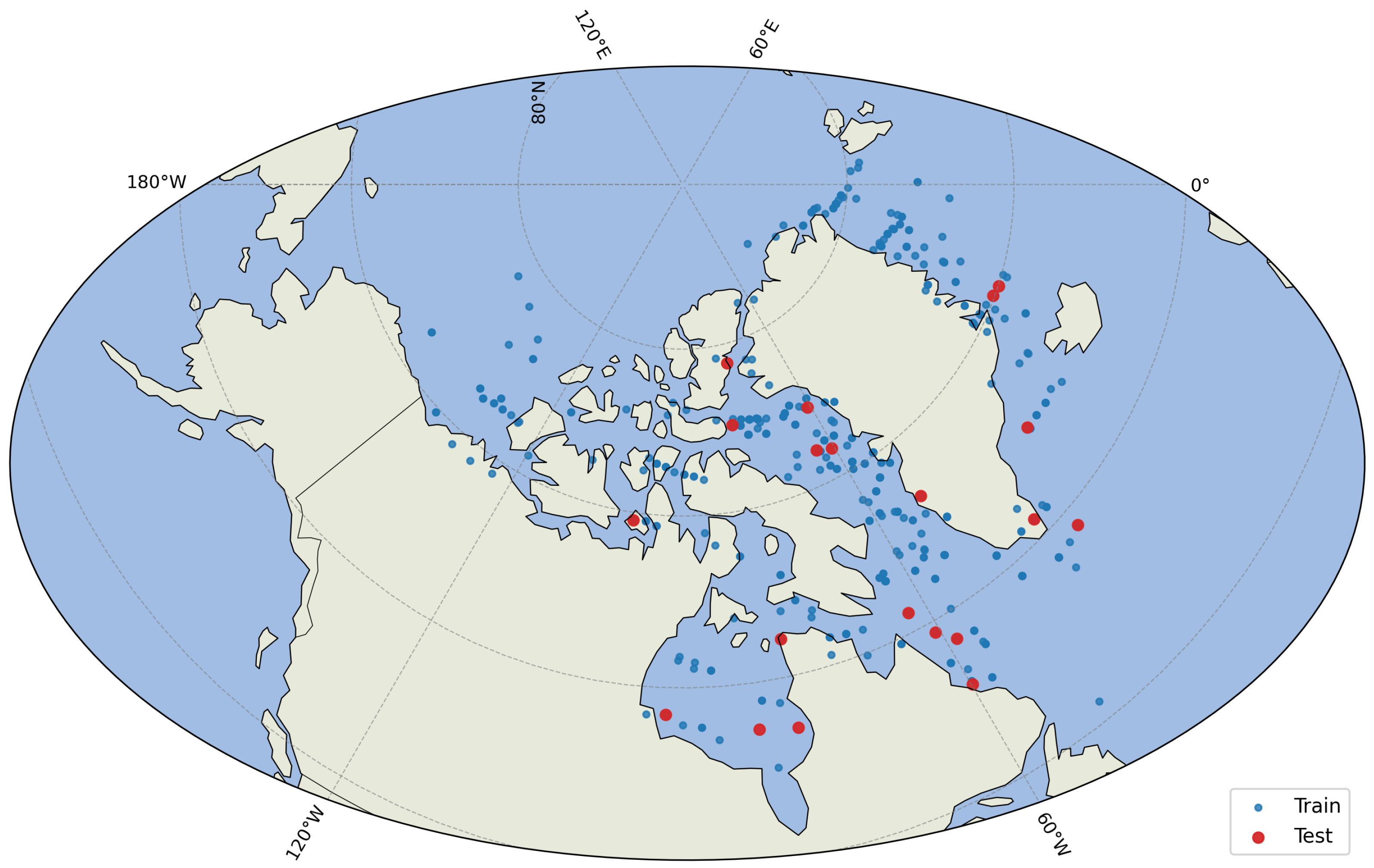
The spatial distribution of the training and test scenes is illustrated in Figure 1. The dataset covers a wide Arctic region, and the test scenes are geographically separated from the training scenes to evaluate model generalization across different locations.
Figure 1.
Spatial distribution of the AI4Arctic training and test scenes.
The RTT dataset provides an official split consisting of 512 training scenes and 20 geographically independent test scenes defined by the AutoICE challenge organizers. These test scenes are selected to be spatially separated from the training data in order to evaluate cross-scene generalization under realistic deployment conditions. Following the standard AI4Arctic benchmark protocol, we retain this fixed test set to enable direct comparability with prior studies. In addition, the test set includes 20 scenes, of which 10 correspond to the freezing season and 10 correspond to the melting season. This seasonal balance introduces variability in environmental conditions and SAR backscatter characteristics and supports evaluation of model performance across different sea ice regimes, which have been shown to affect deep learning–based SIC prediction performance under melting-season conditions [31].
3. Materials and Methods
3.1. U-Net Model
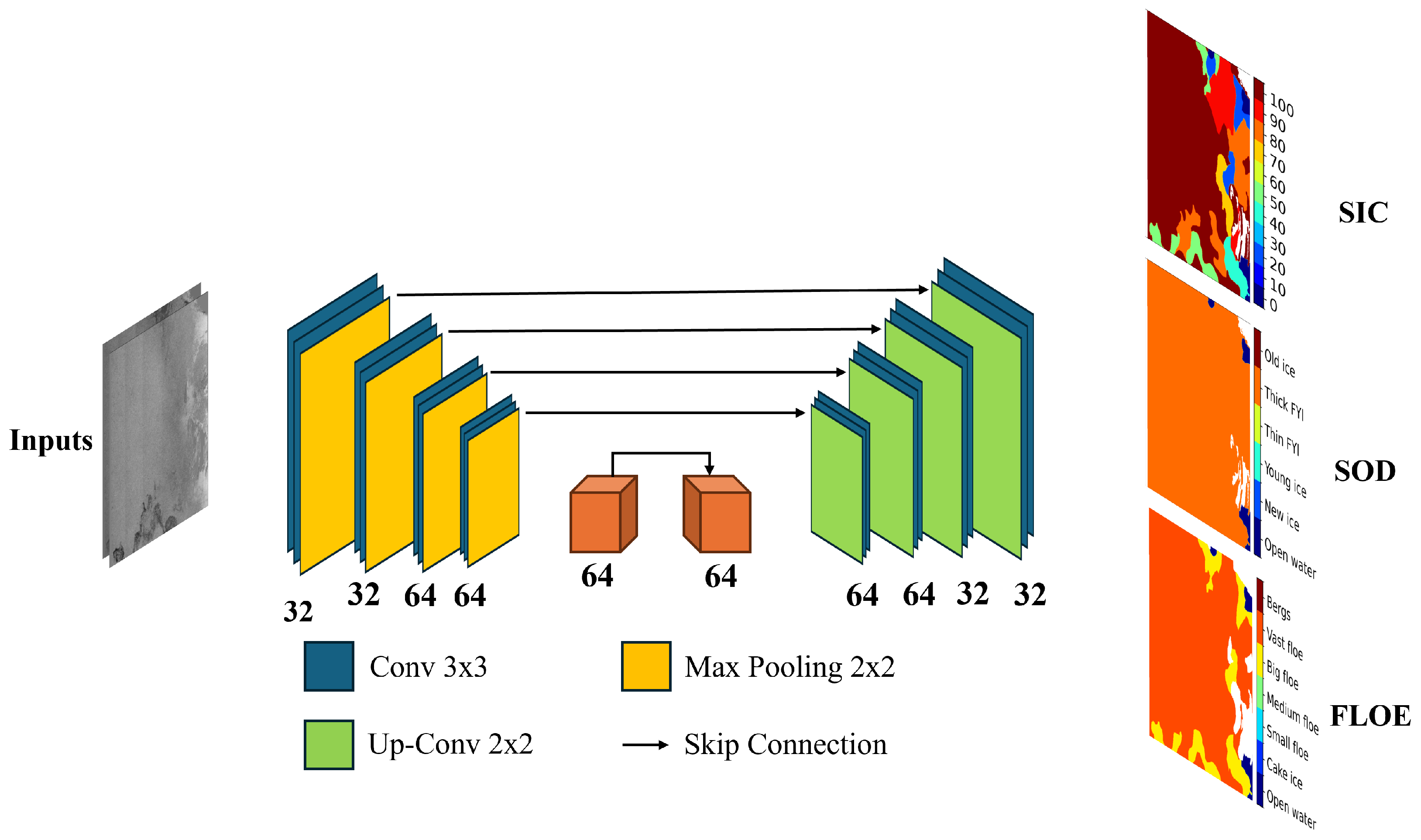
As the main objective of this study is not to develop a new model but to investigate the importance of calibration, we use a U-Net encoder–decoder network as the baseline architecture for multi-task sea ice mapping. The encoder extracts multi-scale features through repeated convolution and downsampling blocks, while the decoder restores spatial resolution through upsampling blocks and skip connections that transfer high-resolution encoder features to the decoder. This design supports accurate localization of boundaries and fine-scale structures in SAR imagery. Figure 2 illustrates the U-Net architecture used in this work.
Figure 2.
U-Net model architecture.
The model outputs three dense segmentation maps for SIC, SOD, and FLOE. The network shares the backbone feature extractor, and produces task-specific logits through three output heads. Each head maps the shared decoder features to the class dimension of its task using a convolution, which yields logits for each chart , where B is the batch size, H and W are the height and width of the input patch, and is the number of classes for task c.
3.2. Loss Functions
Training uses a per-task segmentation loss with four components: cross-entropy with label smoothing, focal cross-entropy, Brier loss, and an entropy-based regularization term. These losses are designed for the AI4Arctic multi-task setting, where the model predicts pixel-wise maps for SIC, SOD, and FLOE, and where the output probabilities are used not only to select a class label, but also to represent prediction confidence. This is important for operational sea-ice products, because low-confidence regions often correspond to uncertain ice regimes such as marginal ice zones, mixed ice types, and boundary transitions, where errors are more likely and decision-making benefits from uncertainty awareness.
Let denote logits for a given task, and let denote the ground-truth labels with ignore index . Define the valid set over all pixels in the batch. Let
denote the softmax probability (the predicted probability for class k at pixel i) assigned to class k at pixel index i, where is the logit predicted for class k at pixel i, K is the total number of classes for the task, and the summation over j normalizes the exponentiated logits across all classes so that and .
In multi-class sea-ice mapping, calibration errors often appear as overconfident wrong predictions, particularly for minority or visually ambiguous categories such as small floes, fragmented ice, or transition zones between open water and ice. For this reason, we evaluate calibration-aware objectives that regularize predicted probabilities to improve calibration rather than optimizing only classification accuracy.
3.2.1. Cross-Entropy Loss with Label Smoothing
We use multi-class cross-entropy (CE) as the main supervision term for each task. CE encourages the correct class probability to increase relative to other classes, which improves segmentation accuracy. However, CE alone is known to promote overconfident probability outputs, because it strongly rewards assigning near-one probability to the predicted class even when the input is uncertain or labels are noisy. This issue is relevant for AI4Arctic, since ice chart labels are polygon-based and may not perfectly represent fine-scale SAR variability. Let K denote the number of classes for the current task (e.g., for SIC, for SOD, and for FLOE), and let be the ground-truth class label at pixel index i. The network outputs logits for each class , which are converted to probabilities through the softmax function. Pixels with an ignore label are excluded using the valid index set , and denotes the number of valid pixels used in the loss.
To reduce overconfidence and improve generalization under label uncertainty, we apply label smoothing with parameter (set to in our experiments). Instead of using a hard one-hot target, label smoothing defines a softened target distribution :
where represents the target probability assigned to class k at pixel i. The label-smoothed cross-entropy loss is then computed as
This loss encourages the model to assign high probability to the correct class and prevents probabilities from collapsing to exactly one, which helps reduce overconfident predictions.
3.2.2. Focal Cross-Entropy Loss
Sea ice segmentation on AI4Arctic is affected by class imbalance and uneven difficulty across pixels. Large homogeneous regions, such as open water or dominant ice regimes, are easy to classify and contribute a large portion of the gradient, while rare classes and boundary regions contribute less, even though they are also very important for practical interpretation. To address this, we add focal cross-entropy, which downweights well-classified pixels and focuses training on harder examples [32].
The focal loss is
where is the focusing parameter. When a pixel is already classified with high confidence (), the factor becomes small, and its contribution to the loss decreases. In contrast, misclassified or uncertain pixels have smaller and receive a larger loss weight. This shifts training toward boundary regions and minority ice categories, which can improve calibration indirectly by helping the model to reduce high-confidence errors on hard samples.
3.2.3. Brier Loss
While CE and focal loss are likelihood-based objectives that mainly optimize class separation, they do not directly penalize confidence misalignment. To improve calibration, we use the multi-class Brier loss [33], which measures squared error between the predicted probability vector and the one-hot target distribution. For pixel i, the one-hot target indicator is
where denotes the indicator function, if the ground-truth class at pixel i equals k, and otherwise. The Brier loss is computed over valid pixels as
The Brier loss penalizes incorrect confidence even when the predicted class is correct, because it evaluates the full probability distribution. In our sea-ice setting, this is useful because it discourages inflated confidence in ambiguous regions and reduces the probability of producing sharp but unreliable predictions.
3.2.4. Entropy Penalty
Deep neural networks, including U-Net architectures, trained with standard objectives can become overly confident [25]. To regularize confidence, we add an entropy-based penalty computed from the predictive distribution [34]. The per-pixel predictive entropy is defined as
where is the entropy at pixel i. We compute the entropy penalty by averaging across valid pixels:
Unlike CE and focal loss, which push probability mass toward the correct class, the entropy term controls the sharpness of the predicted softmax class-probability distribution and reduces excessive certainty. This is particularly helpful for AI4Arctic, where label uncertainty and mixed ice regimes can make overly confident predictions unreliable.
3.2.5. Per-Task Combined Loss and Multi-Task Objective
Each loss component targets a different source of miscalibration and error. CE provides the main discriminative signal, focal loss increases attention to hard and minority pixels, Brier loss directly penalizes probability miscalibration, and entropy regularization limits overconfident distributions. Their combination, therefore, links segmentation quality with probability reliability, which is essential when confidence maps are used to interpret uncertainty across SIC, SOD, and FLOE products. For each chart , the task loss is a weighted combination that matches our training code:
The final training objective sums up tasks:
We use a global and chart-specific weights for the other terms, which allows different regularization strength across SIC, SOD, and FLOE. Overall, these losses convert the U-Net from an accuracy-optimized model into a calibration-aware model that produces more meaningful confidence maps for sea-ice decision support.
The loss weights and focal parameters mentioned in Table 1 were selected through cross-validation experiments to balance segmentation accuracy and calibration across SIC, SOD, and FLOE. These weights combine complementary effects: CE provides class separation, focal emphasizes hard pixels, Brier penalizes miscalibrated probabilities, and the entropy term reduces extreme confidence peaks. Together, they aim to improve both segmentation quality and calibration for SIC, SOD, and FLOE.
Table 1.
Chart-specific loss weights and focal parameters used in training.
The weighting coefficients associated with the calibration-oriented loss components were obtained through a cross-validation-based hyperparameter tuning procedure. A grid-search strategy explored task-specific weight combinations for the Brier, focal, and entropy loss terms across the SIC, SOD, and FLOE outputs. Each candidate configuration was trained under the same Monte Carlo cross-validation protocol used throughout this study. The resulting models were assessed on the validation splits using both segmentation performance metrics (SIC R2, SOD F1, FLOE F1) and ECE. Final weight values were selected based on CS together with validation ECE in order to jointly account for segmentation accuracy and probabilistic reliability.
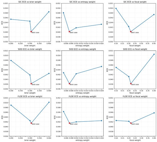
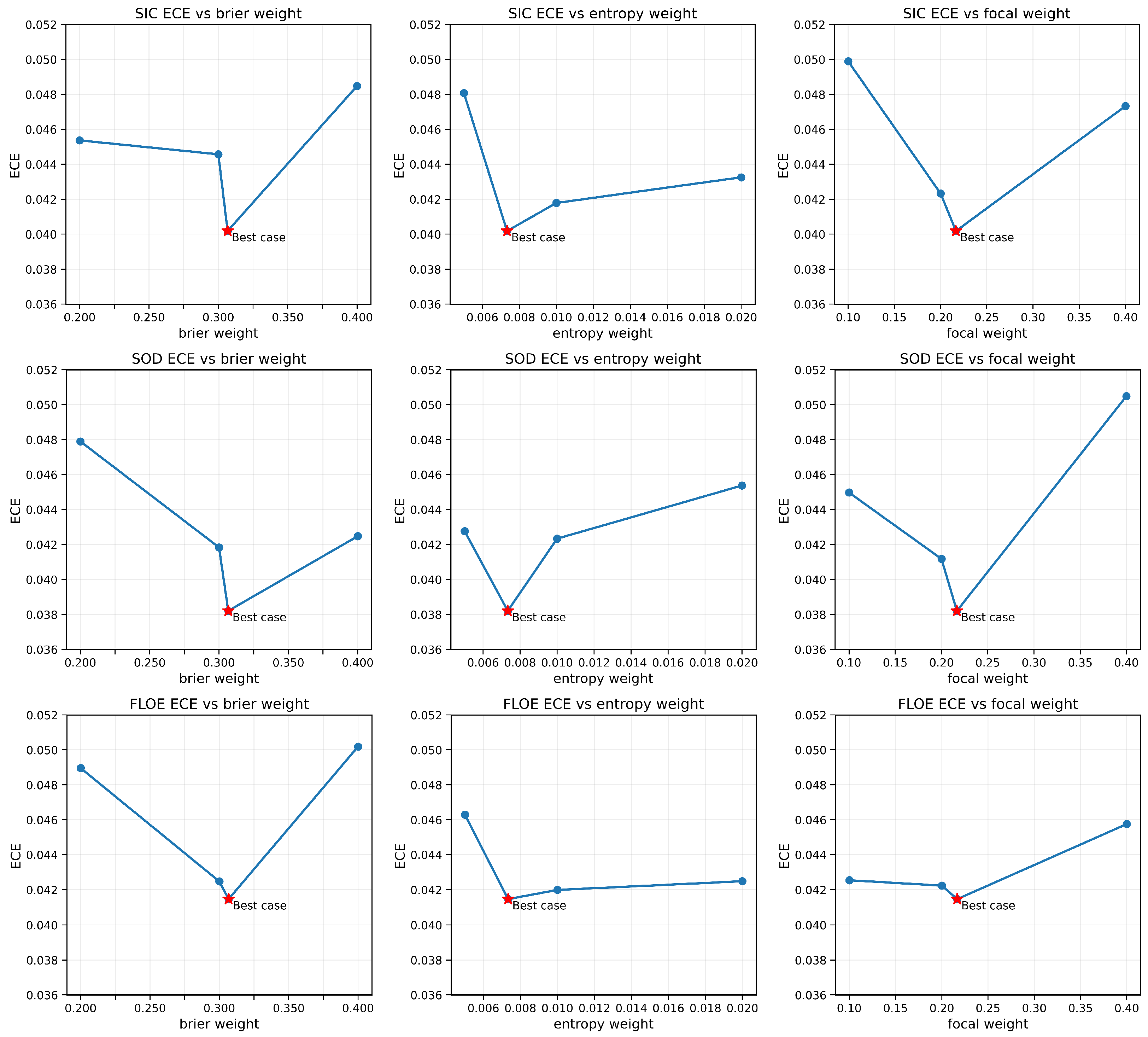
To check how sensitive the calibration is to the exact loss weights in Table 1, we ran a sensitivity study where we varied one loss weight at a time (Brier, entropy, or focal) over the values tested in our sweep, while keeping the rest of the training setup unchanged. Each setting was retrained using the same Monte Carlo cross-validation procedure, and we report the mean ECE for SIC, SOD, and FLOE.
Figure 3 summarizes the ECE trends for each task under the three weight sweeps. In every panel, the red star marks the selected best-case weight from Table 1. Across all tasks, ECE changes gradually with weight adjustments and stays within a limited band, which suggests that the chosen weights do not rely on a single fragile setting and that calibration remains stable under moderate perturbations of the loss weights.
Figure 3.
Sensitivity of model performance to variations in focal, Brier, and entropy loss weights. The red star denotes the selected configuration reported in Table 1.
3.3. Calibration Metrics
We evaluate probability reliability using reliability diagrams and scalar calibration metrics computed on the test set. For each pixel i, the model outputs a probability vector over the K classes of the corresponding task. The predicted class label is
and the associated confidence score is defined as the maximum predicted probability,
To construct reliability diagrams, we partition maximum softmax probability into M confidence bins (e.g., ) based on , and compare the actual accuracy in each bin with the mean confidence. For bin , the accuracy and confidence are computed as
where is the number of pixels in bin , is the ground-truth label. A perfectly calibrated model follows the diagonal relation across bins.
We summarize calibration using the expected calibration error (ECE), which measures the average mismatch between confidence and accuracy across bins [25]:
where N is the total number of evaluated pixels. Lower ECE values indicate better calibration. We report ECE separately for SIC, SOD, and FLOE to capture task-dependent differences in confidence behavior.
3.4. Training Strategy
Model training follows a scene-level Monte Carlo cross-validation protocol. For each run, we randomly select 20 scenes from the RTT dataset as validation scenes, and use the remaining scenes for training. We repeat this procedure for 10 splits to reduce sensitivity to a single train/validation partition and to obtain more reliable performance estimates.
Due to the large spatial extent of AI4Arctic scenes, training is performed using random patch sampling. Each training iteration returns one mini-batch of patches and the corresponding labels for SIC, SOD, and FLOE. We train for 60 epochs, with 500 iterations per epoch and batch size 16. Data augmentation is applied during training using random horizontal and vertical flips, random rotations, and random scaling, which increases sample diversity and improves robustness to orientation and scale variations in SAR textures.
During optimization, the network is trained in a multi-task setting where SIC, SOD, and FLOE are learned jointly. For each mini-batch, the model produces three logit maps (one per task), and the total training objective is computed as the sum of task-specific losses. Each task loss combines cross-entropy with label smoothing as the primary supervision term, and includes additional focal, Brier, and entropy components with chart-dependent weights. This design allows the training objective to balance segmentation accuracy and probability quality. The combined loss is backpropagated to update shared encoder–decoder parameters and task-specific heads simultaneously.
Optimization uses stochastic gradient descent (SGD) with momentum () and weight decay (). At the end of each epoch, the model is evaluated on the validation scenes, and the best checkpoint is selected based on the validation score.
All model and hyperparameter selections, including loss-weight tuning and the choice of the final training objective, were performed exclusively using validation scenes from the Monte Carlo cross-validation splits of the RTT training set. The held-out test set was not accessed during model selection and was used only once for final performance evaluation. This protocol prevents test-set leakage and ensures that reported test results reflect unbiased generalization performance.
4. Evaluation Metrics
Model performance is evaluated using task-specific metrics, together with a combined score that summarizes overall multi-task performance.
To evaluate SIC predictions, we use the coefficient of determination (), which measures how well the predicted values explain the variance in the reference data. The score is defined as
where and denote the ground-truth and predicted SIC values at pixel i, respectively, is the mean of the ground-truth SIC values over all valid pixels, and N is the total number of evaluated pixels. An value of 1 indicates perfect agreement, while lower values indicate increasing prediction error relative to the variance of the reference data.
For SOD and FLOE, we use the F1 score, which balances precision and recall. For a given class, precision and recall are defined as
where , , and denote the numbers of true positives, false positives, and false negatives, respectively. The F1 score is then computed as
To provide a single scalar measure of overall performance across all sea ice products, we report a combined score that aggregates SIC, SOD, and FLOE metrics using task-specific weights. The combined score is defined as
Higher weights are assigned to SIC and SOD to show their greater operational importance and relative difficulty.
5. Results
5.1. Quantitative Results
Table 2 and Table 3 present an ablation study of the proposed composite objective, where the U-Net model is trained using different combinations of the four loss components (CE, focal, Brier, and entropy). This analysis evaluates the individual and joint contributions of each loss term to segmentation accuracy and calibration performance, and investigates whether retaining all components is necessary for optimal multi-task mapping. Overall, all loss variants achieve strong and consistent cross-validation performance, with relatively small standard deviations across splits, which indicates stable training behavior.
Table 2.
Cross-validation performance (Avg ± Std) for different loss functions.
Table 3.
Test performance for different loss functions.
For cross-validation, the CE loss achieves a CS of . Adding calibration-oriented terms produces comparable or slightly improved results depending on the task. In addition to improving mean performance, several loss combinations reduce the cross-validation standard deviation, which indicates more consistent optimization and improved robustness across Monte Carlo splits. For example, CE + Brier reduces the CS variability from to , and the full objective (CE + Brier + focal + entropy) further maintains a lower variability of . This reduction in dispersion suggests that the additional loss terms act as regularizers, which stabilize training dynamics and reduce performance fluctuations caused by scene-to-scene diversity.
The highest cross-validation CS is obtained by the full objective (CE + Brier + focal + entropy), which reaches and also achieves the best FLOE score (). This suggests that combining hard-example emphasis (focal loss) with probability-regularization terms (Brier and entropy) can improve floe-size segmentation and preserve competitive SIC and SOD performance.
On the test set, the CE loss achieves a CS of . All modified objectives outperform this baseline in terms of CS, which confirms that auxiliary loss terms improve generalization. The best overall test performance is achieved by CE + Brier + focal + entropy, which obtains the highest CS of . This configuration also produces strong results across all tasks, with SIC , SOD F1 , and FLOE F1 . Compared with the CE loss, the full objective improves CS by , with the largest gain observed for FLOE, which increases from to . These results indicate that FLOE classification benefits the most from the additional loss components.
Across all test experiments, several loss combinations show competitive performance. CE + focal provides the highest SIC score (), while CE + focal + entropy achieves the highest FLOE score (). However, the full loss combination provides the most balanced improvement across tasks and achieves the best overall CS, which makes it the most effective configuration for multi-task sea ice mapping in this study.
5.2. Qualitative Results
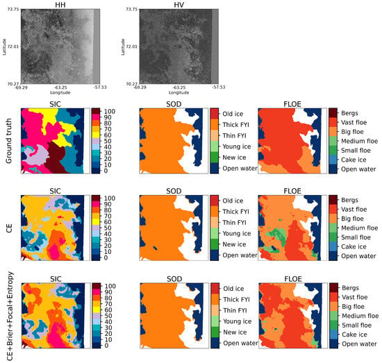
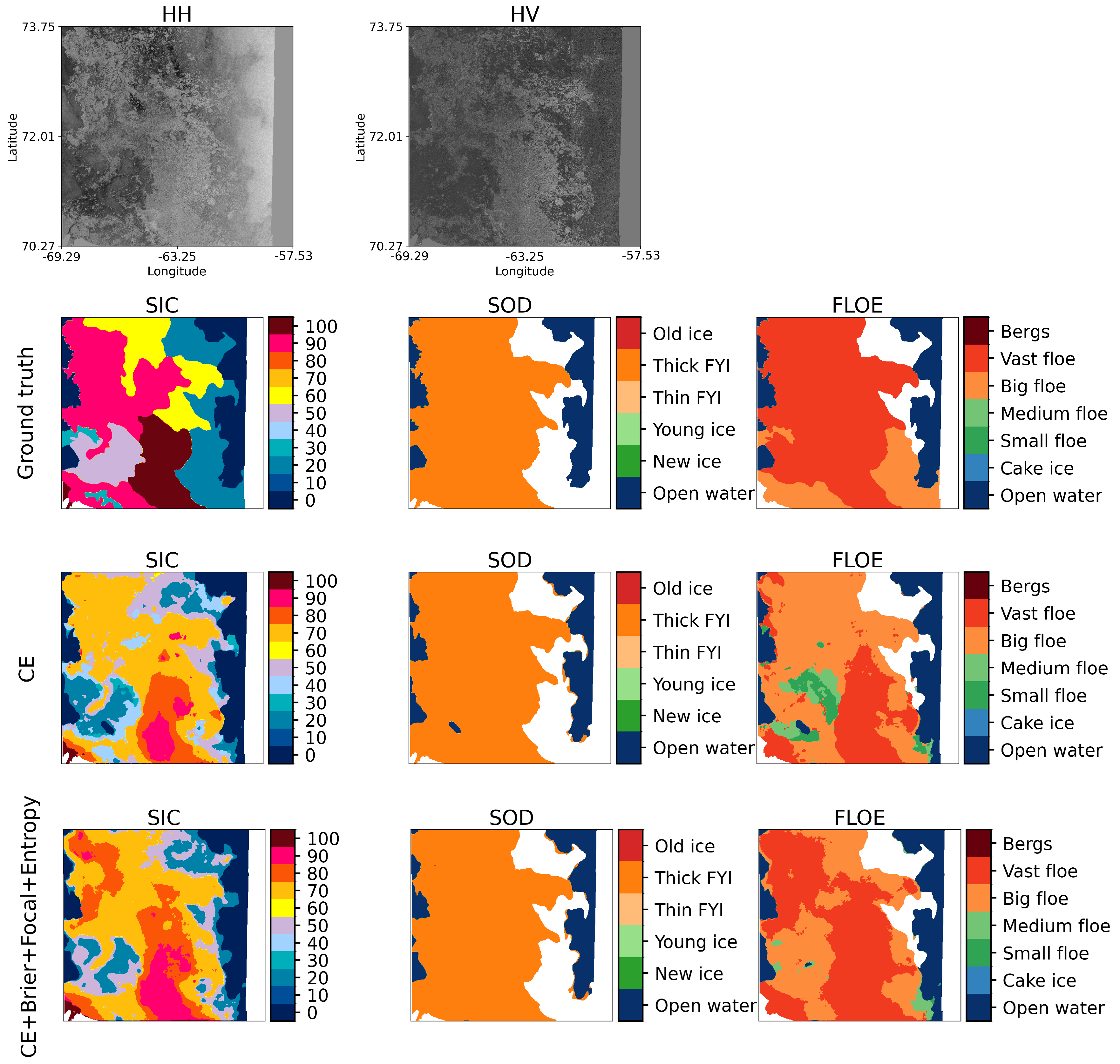
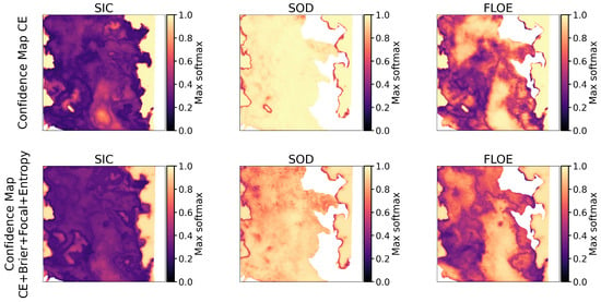
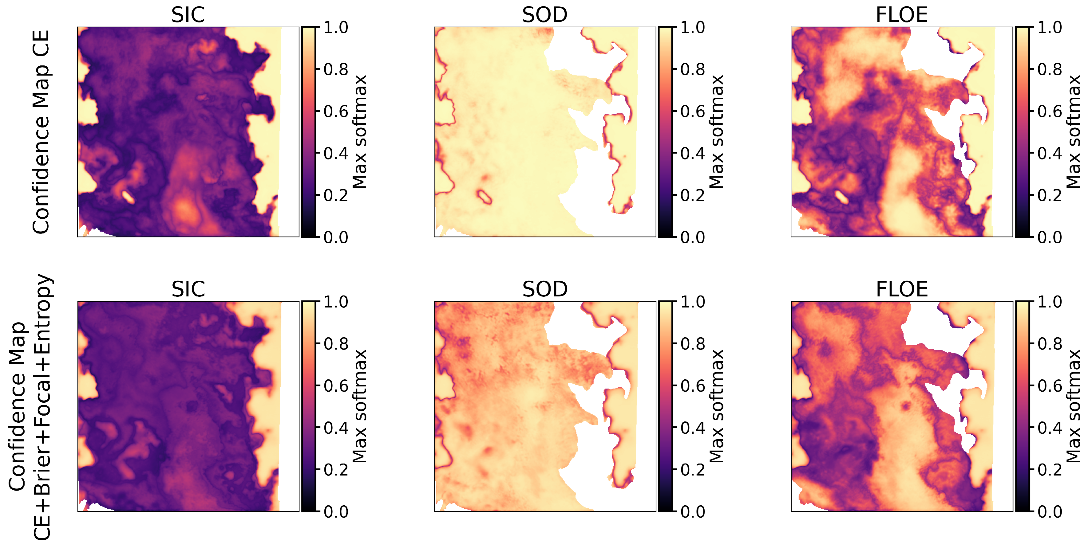
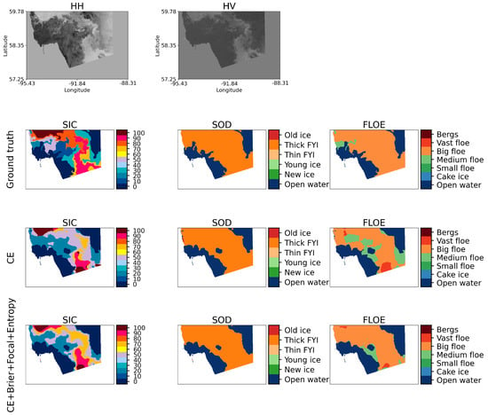
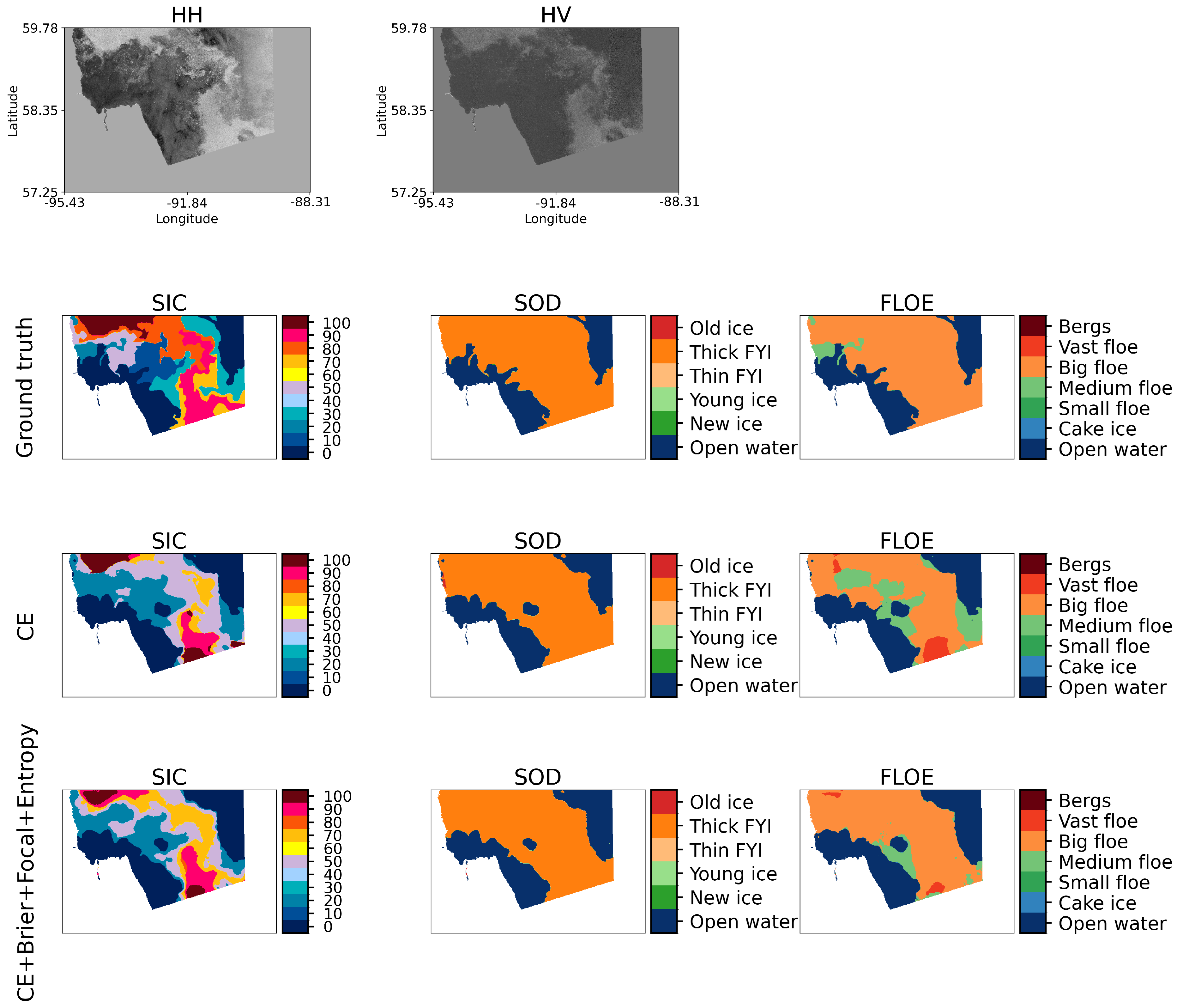
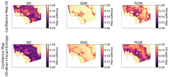
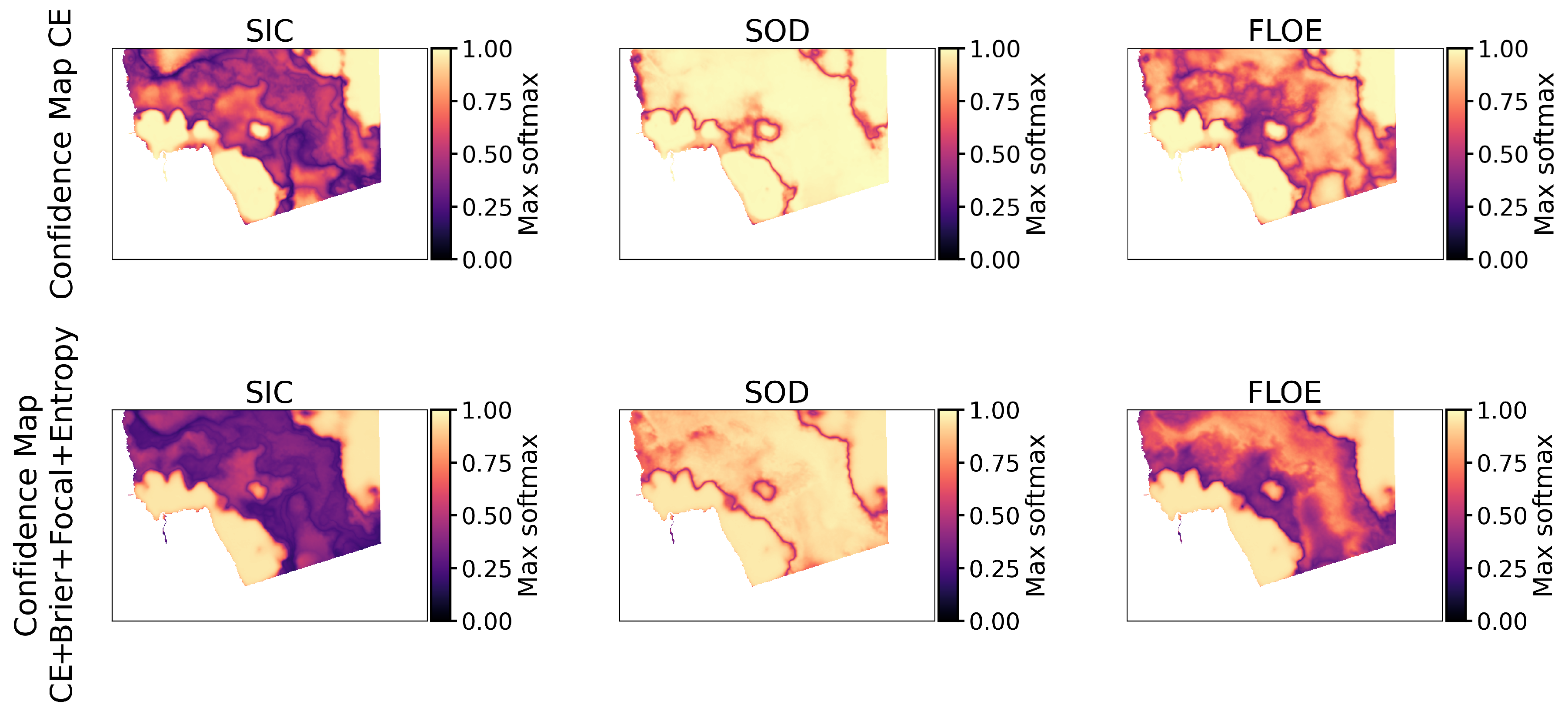
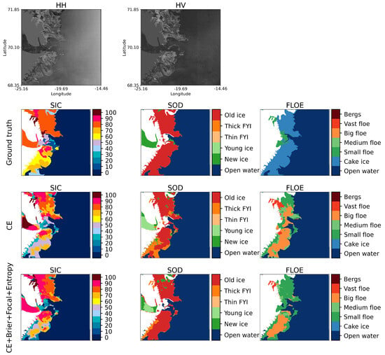
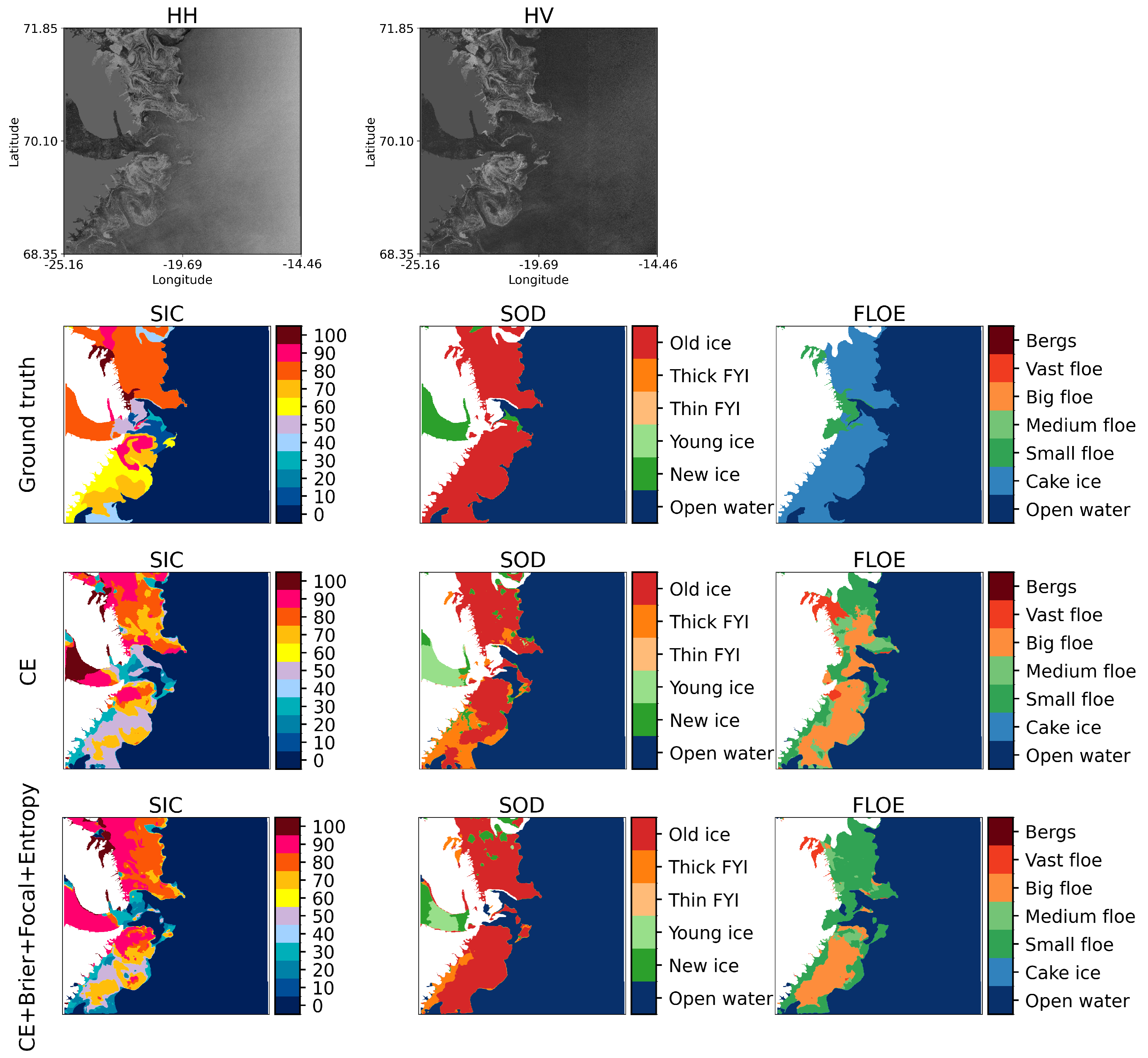
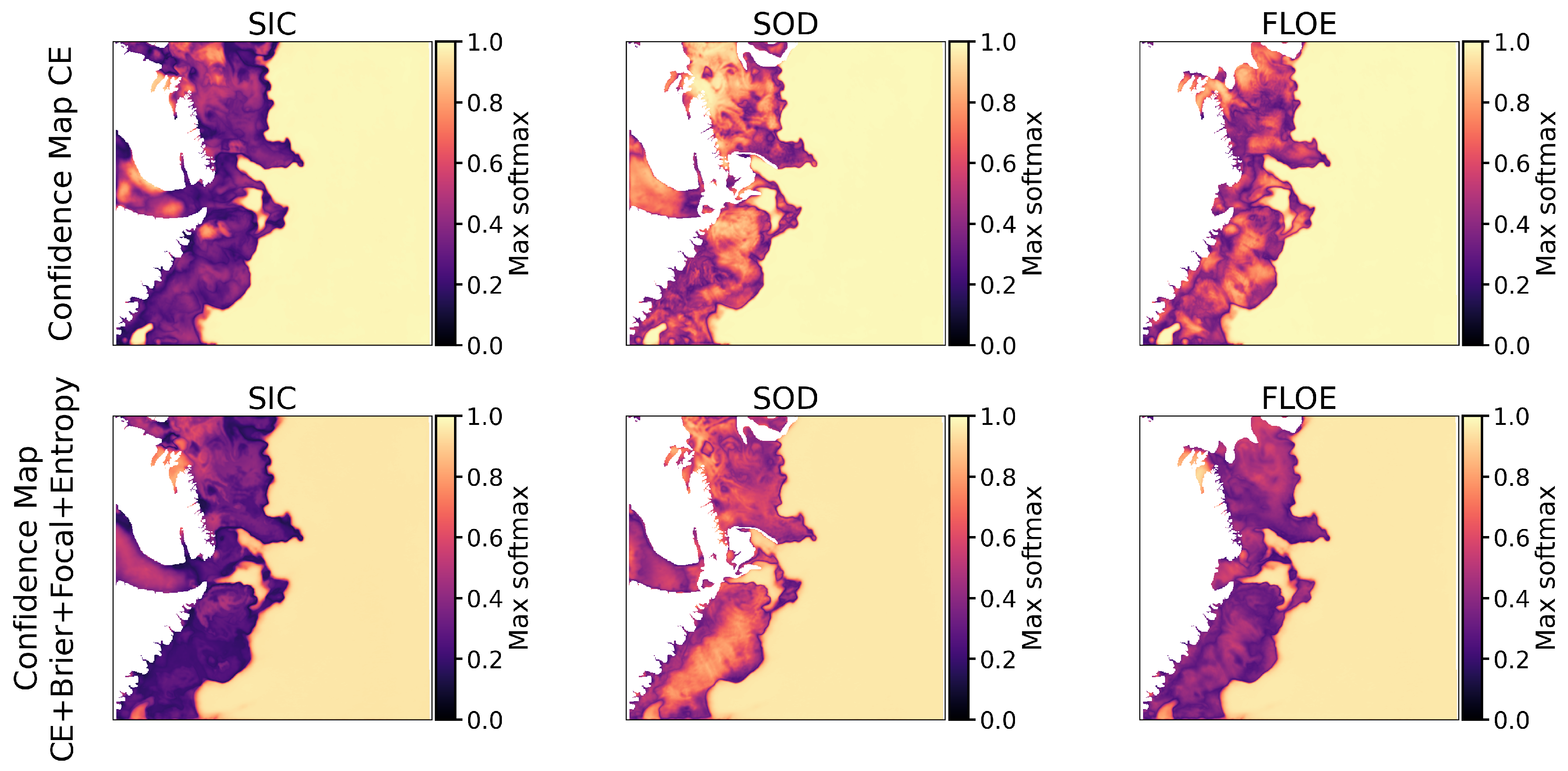
Figure 4, Figure 5, Figure 6, Figure 7, Figure 8 and Figure 9 show qualitative results for three representative test scenes, including the Sentinel-1 HH/HV inputs, the ground-truth ice chart labels, and the corresponding predictions from the CE and CE + Brier + focal + entropy losses. In addition, each figure includes confidence maps (maximum softmax probability) for SIC, SOD, and FLOE, which provide a spatial view of prediction certainty and help interpret model behavior near boundaries and mixed-ice regimes. Across all scenes, both objectives reproduce the main sea ice versus open-water structure, but the calibration-aware objective produces segmentation outputs that are visually closer to the reference charts and confidence patterns that are more spatially meaningful.
Figure 4.
Ground truth and model predictions of the 20180716T110418-cis-prep scene.
Figure 5.
Confidence maps of loss functions for the 20180716T110418-cis-prep scene.
Figure 6.
Ground truth and model predictions of the 20200719T123046-cis-prep scene.
Figure 7.
Confidence maps of loss functions for the 20200719T123046-cis-prep scene.
Figure 8.
Ground truth and model predictions of the 20201013T080448-dmi-prep scene.
Figure 9.
Confidence maps of loss functions for the 20201013T080448-dmi-prep scene.
For SIC, the CE loss often shows noisy class transitions and scattered misclassified regions inside large ice areas, especially in heterogeneous zones where the SAR texture varies gradually. This effect appears clearly in Figure 4, where CE introduces fragmented concentration patches that do not follow the smoother chart polygons. The calibration-aware objective reduces this speckle-like behavior and produces more coherent concentration fields, with cleaner boundaries between dominant concentration regimes. A similar trend is observed in Figure 6, where the CE prediction contains more small-scale inconsistencies along the ice edge, while the combined loss achieves a more continuous concentration gradient and fewer isolated class islands. These qualitative differences match the quantitative results, where the combined loss provides stronger generalization and improved combined score.
For SOD, both losses typically identify the prevailing ice development stage over large regions, which indicates that this task is less sensitive to the choice of loss. However, CE tends to introduce boundary noise in areas close to the marginal ice zone. In Figure 8, the CE prediction produces irregular class patches along transition areas, while the combined loss produces smoother and more stable SOD regions that better match the chart structure. This improvement is important because SOD classes often show gradual physical transitions, and excessive spatial fragmentation reduces interpretability for operational use.
For FLOE, the difference between objectives is the most pronounced. Under CE training, floe-size predictions show strong patch-level variability, with frequent switches between neighboring floe categories inside regions that should be more homogeneous. This behavior is visible in all three scenes, particularly in Figure 4, where CE produces scattered small-floe and medium-floe regions within dominant floe regimes. The calibration-aware objective substantially reduces this instability and produces clearer regional separation between floe classes, with fewer isolated misclassifications. In Figure 6, the combined loss also improves the continuity of floe-size zones and better aligns the predicted class structure with the reference map. These observations are consistent with the test-set improvements for FLOE F1 reported in Table 3, which indicates that FLOE benefits the most from the proposed objective.
The confidence maps shown in Figure 5, Figure 7 and Figure 9 provide additional insight into why the calibration-aware objective performs better. For both objectives, confidence tends to be high in uniform interior regions (large open-water areas or dominant ice regimes) and lower near boundaries, which is expected because mixed pixels and label uncertainty are more common at transitions. However, the CE confidence maps are often overly saturated, with large areas assigned very high confidence even when the corresponding segmentation contains visible errors or fragmented patterns. In contrast, the calibration-aware objective produces confidence maps with sharper spatial contrast: uncertainty is concentrated near ice edges, narrow channels, and mixed-regime zones, while homogeneous regions remain confidently predicted. This behavior is most evident for FLOE, where the combined loss produces both smoother segmentation and confidence fields that better reflect scene complexity. Overall, these qualitative results support the conclusion that calibration-aware loss design improves not only the visual consistency of SIC/SOD/FLOE maps but also the spatial reliability of confidence estimates, which is critical for risk-aware interpretation of automated sea ice products.
5.3. Calibration Results
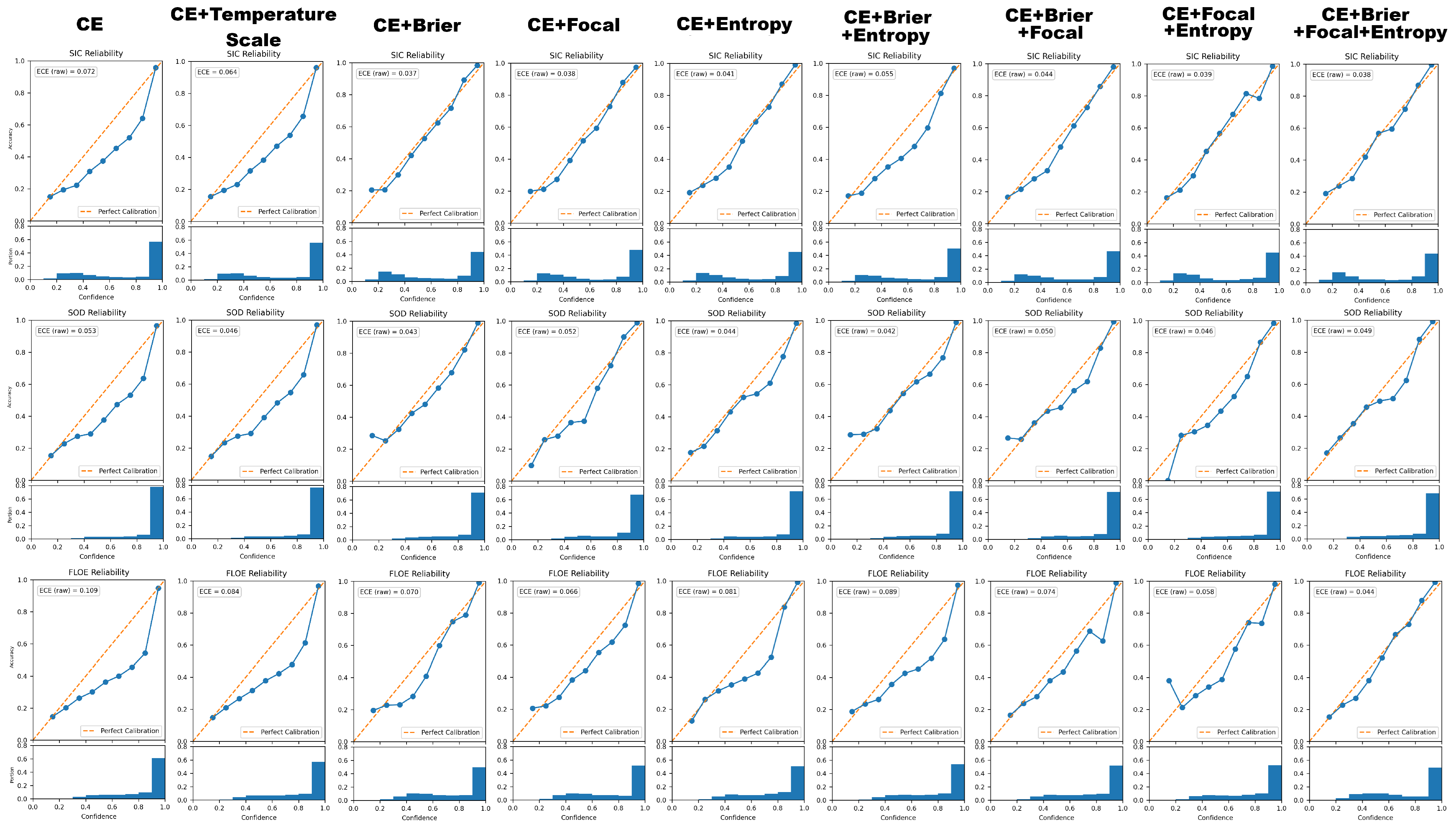
Table 4 and Figure 10 summarize the calibration behavior of the U-Net model under different loss configurations using expected calibration error (ECE) and reliability diagrams for SIC, SOD, and FLOE. The CE loss exhibits noticeable overconfidence across all tasks, which is reflected by relatively high ECE values of for SIC, for SOD, and for FLOE. This effect is also visible in the reliability plots, where the accuracy curve lies below the diagonal line in the high-confidence regime, which indicates that predicted probabilities are higher than the true accuracy.
Table 4.
ECE of different loss functions on the test dataset.
Figure 10.
Calibration plots of different loss functions for SIC, SOD, and FLOE computed on the test dataset. The blue line represents the calibration curve obtained by grouping predictions into confidence bins and plotting the observed accuracy against the predicted confidence for each bin.
Introducing calibration-oriented loss components substantially improves probability reliability. Adding the Brier loss produces a clear reduction in ECE for all three tasks and decreases SIC ECE from to , SOD ECE from to , and FLOE ECE from to . This improvement is consistent with the role of the Brier term, which penalizes the squared difference between predicted probabilities and the one-hot target distribution and therefore discourages overly confident incorrect predictions.
In addition to the proposed training-time calibration strategies, we also evaluated a standard post-processing calibration approach based on temperature scaling applied to a CE-trained model. Temperature scaling [25] is widely adopted as a lightweight calibration method that adjusts predicted probabilities without modifying the underlying decision boundaries. As shown in Table 4, temperature scaling reduces SIC ECE from 0.072 to 0.064, SOD ECE from 0.053 to 0.046, and FLOE ECE from 0.109 to 0.084. However, training-time calibration using hybrid loss functions consistently achieves substantially lower ECE across all tasks compared to temperature scaling. For instance, CE + Brier reduces SIC ECE to 0.037, while the full objective (CE + Brier + focal + entropy) further improves FLOE calibration to 0.044 compared to 0.084 achieved through post-processing.
Focal loss also reduces ECE relative to CE, particularly for FLOE (), which suggests that emphasizing hard pixels can indirectly improve confidence calibration in the most challenging task. Entropy regularization provides moderate improvements compared with CE, but it is less effective than Brier-based objectives when used alone. The most consistent calibration improvements are achieved when multiple loss components are combined. In particular, the full objective (CE + Brier + focal + entropy) yields the lowest FLOE ECE () and maintains low ECE for SIC () and SOD (). The corresponding reliability curves are closer to the diagonal across a wider confidence range, which indicates improved alignment between predicted confidence and actual correctness.
From an operational perspective, ECE quantifies the expected difference between predicted confidence and observed accuracy. For example, an ECE of 0.109 implies that a prediction made with 80% confidence may be correct only about 69% of the time on average. Reducing FLOE ECE to 0.044 decreases this mismatch, such that an 80% confidence prediction is expected to be correct approximately 76% of the time. In practical deployment, improved calibration allows confidence maps to serve as more reliable indicators of uncertainty in downstream navigation and risk-assessment workflows.
Overall, these results show that calibration-focused losses can significantly reduce overconfidence in multi-task sea ice segmentation. The improvements are most pronounced for FLOE, which also shows the largest calibration error under the CE loss. This behavior highlights the importance of explicitly optimizing probability quality in addition to segmentation accuracy, especially for difficult and imbalanced sea ice products.
5.4. Convergence Behavior
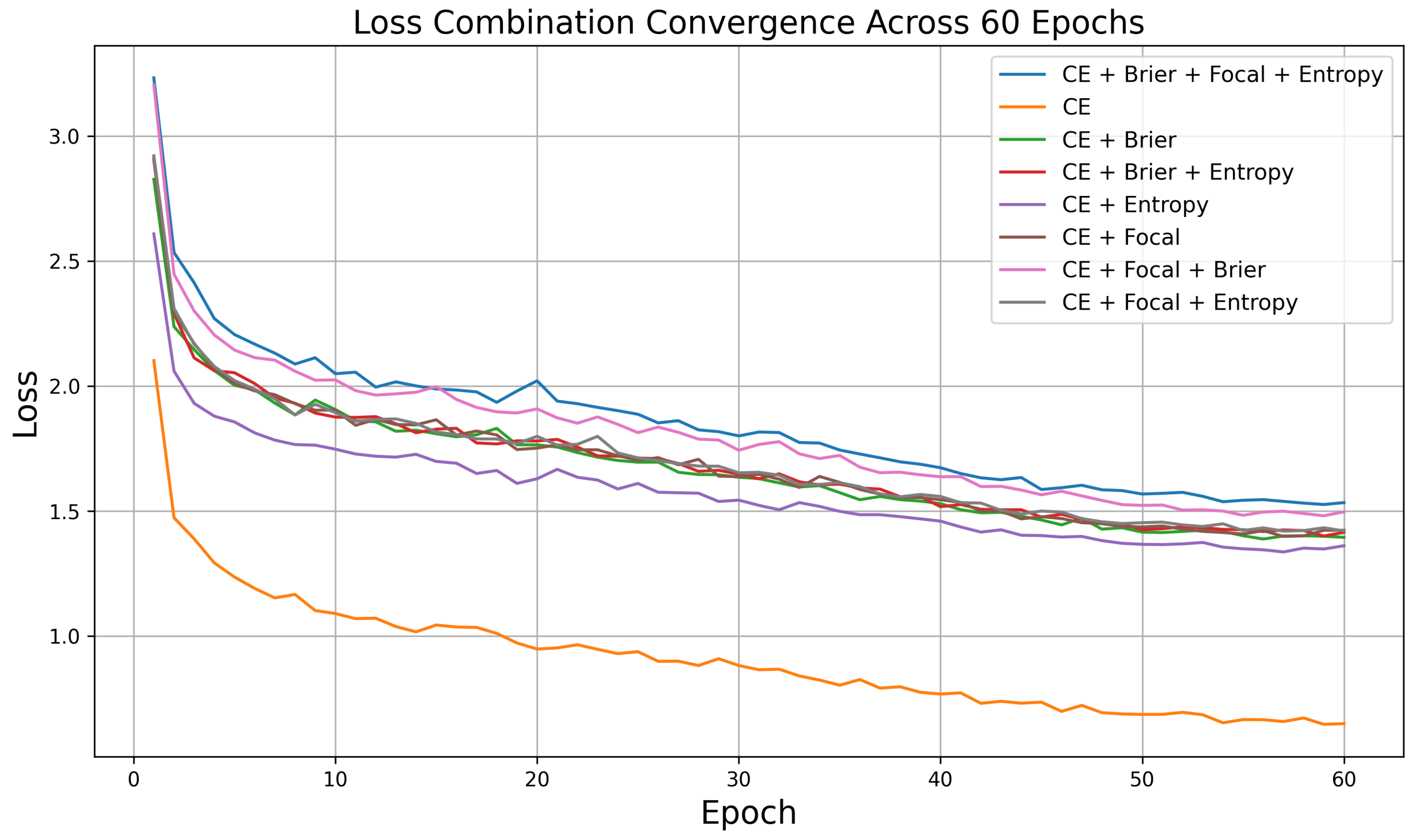
To investigate whether the introduction of multiple loss components affects optimization efficiency, we analyzed the training convergence behavior of different loss configurations over a fixed 60-epoch schedule. As illustrated in Figure 11, all evaluated multi-loss formulations show convergence patterns comparable to the baseline cross-entropy loss. In particular, the validation loss decreases consistently throughout training without evidence of delayed convergence or optimization instability when additional terms such as Brier, focal, or entropy losses are added.
Figure 11.
Training convergence of different loss combinations across 60 epochs.
These observations indicate that the proposed multi-task, multi-loss strategy does not significantly increase the complexity of the optimization process during training. Although additional loss terms introduce a modest computational overhead during gradient computation in the backward pass, they do not modify the forward inference pathway of the network. Consequently, inference-time latency and deployment-time computational requirements remain identical to those of the baseline cross-entropy model, which supports the suitability of the proposed approach for operational sea-ice monitoring applications.
The additional calibration-oriented loss terms increase the computational cost during training by approximately 20 s per epoch (from 39.8 s to 60.4 s per epoch) due to the extra gradient computations introduced during loss evaluation and backpropagation. All experiments were conducted on a single NVIDIA H100 80GB HBM3 GPU (3g.40gb MIG instance). In contrast, inference time remains effectively unchanged because the proposed calibration components are applied only during optimization and do not alter the network architecture or forward propagation pathway. On 20 held-out test scenes, the mean per-scene forward time is about 4.5 ms for the CE and CE + Brier + focal + entropy losses.
5.5. Seasonal Performance Analysis
Seasonal stratification of model evaluation is essential in Arctic sea ice studies, as demonstrated in recent deep learning–based SIC prediction frameworks that explicitly restrict analysis to the melting season in order to account for thermodynamic regime shifts and associated surface scattering variability across seasonal ice states [35,36]. Sea ice surface characteristics exhibit significant seasonal variability, particularly between the winter freezing period and the summer melting phase. During freeze-up conditions, newly formed ice and relatively uniform thermodynamic growth produce more homogeneous surface textures in synthetic aperture radar (SAR) imagery. In contrast, the melting season introduces wet snow layers, fragmented floe structures, surface melt ponds, and increased roughness variability, all of which affect radar backscatter behavior and increase classification uncertainty.
To evaluate the stability of the proposed calibration-focused loss framework under such environmental variability, we conducted an additional seasonal analysis on the test dataset. The test set contains 20 scenes, where 10 correspond to the freezing season and 10 correspond to the melting season. This seasonal balance enables a controlled comparison of model performance across distinct thermodynamic regimes.
Table 5 and Table 6 summarize SIC, SOD, FLOE, and CS performance for each evaluated loss configuration under freezing-season and melting-season conditions, respectively.
Table 5.
Test performance on freezing season scenes for different loss functions.
Table 6.
Test performance on melting season scenes for different loss functions.
The results show that model behavior varies across seasonal regimes due to differences in ice morphology and surface scattering properties. During the freezing season, most loss configurations achieve comparable SIC performance, while improvements in FLOE classification remain relatively moderate. In contrast, melting-season scenes show larger performance gains in FLOE and SOD metrics when calibration-aware loss components, such as Brier and entropy terms, are introduced.
Importantly, the proposed multi-loss calibration framework maintains stable performance across both seasonal regimes. Loss combinations consisting of calibration-oriented terms show improved consistency in CS values between freezing and melting conditions, which indicates enhanced robustness under environmentally diverse scenarios. This stability is particularly relevant for operational applications, where seasonal variability in sea ice texture may otherwise degrade model reliability and confidence estimation.
Further investigation across additional environmental categories, such as wet versus dry snow conditions or regional ice types, may provide deeper insight into calibration behavior under specific scattering regimes and remains an area for future work.
6. Discussion
This study investigated calibration-aware training objectives for multi-task sea ice mapping on the AI4Arctic dataset, with a focus on improving probability reliability without sacrificing segmentation performance. The quantitative results show that combining the CE loss with focal, Brier, and entropy terms leads to consistent gains in the combined score on the test set. In particular, the full objective (CE + Brier + focal + entropy) provides the best overall generalization, which suggests that these loss components complement each other by addressing different aspects of the learning problem. CE drives discriminative class separation, focal loss increases emphasis on difficult and minority pixels, and Brier/entropy terms regulate the probability distribution to reduce overconfident predictions.
A key observation is that FLOE benefits the most from the proposed losses, both in accuracy and calibration. FLOE segmentation is typically more ambiguous than SIC and SOD because floe-size boundaries can be visually subtle in SAR imagery, and the class distribution is often highly imbalanced. The test results show a clear improvement in FLOE F1 when additional loss terms are used, and the calibration analysis reveals that FLOE has the largest baseline ECE under CE training. The reduction of FLOE ECE from (CE) to (full objective) indicates that calibration-focused losses can substantially improve the trustworthiness of floe-size predictions, which is important for operational use cases that require reliable confidence estimates.
The cross-validation statistics further highlight the stabilizing effect of the proposed objective. Several configurations reduce the standard deviation of the combined score across Monte Carlo splits, which indicates lower sensitivity to the specific validation-scene selection and more consistent optimization. This effect is particularly evident when Brier loss is included, which supports the interpretation that probability-based penalties act as regularizers and reduce performance variability across different training runs. More stable training is valuable in the AI4Arctic setting because scenes differ strongly in geographic region, seasonal conditions, and ice types.
Qualitative comparisons support the quantitative trends. The model trained with the full objective produces SIC maps with smoother and more coherent spatial patterns, and FLOE maps with fewer scattered misclassifications and clearer regional separation. For SOD, both CE and the full objective achieve similar large-scale patterns, but the combined loss reduces local noise near complex boundaries, which is consistent with its lower calibration error and improved generalization.
An additional qualitative insight is provided by the confidence maps shown in Figure 5, Figure 7 and Figure 9. In general, high-confidence regions align with homogeneous areas such as open water and dominant ice regimes, while lower confidence occurs near the marginal ice zone, narrow leads, and mixed-ice transitions where SAR texture is ambiguous and label uncertainty is higher. However, the CE baseline often produces overly saturated confidence patterns, where large areas remain highly confident even when the corresponding segmentation contains fragmented or noisy class assignments. In contrast, the calibration-aware objective achieves confidence maps with more meaningful spatial structure, where uncertainty is concentrated around boundaries and heterogeneous zones, and confidence remains high mainly in stable regions. This behavior is consistent with the lower ECE values reported in Table 4 and indicates that the proposed loss combination improves not only segmentation accuracy but also the reliability of pixel-wise confidence.
Overall, the results demonstrate that calibration-aware loss design is an effective and lightweight approach to improve both predictive performance and probability reliability for multi-task sea ice mapping on AI4Arctic. The improvements are most pronounced for FLOE, which indicates that confidence calibration is especially important for challenging and imbalanced sea ice products.
It is also important to consider the role of label uncertainty in the AI4Arctic dataset when interpreting calibration improvements. The reference SIC, SOD, and FLOE labels are derived from operational ice charts, which are defined at the polygon level and may not capture fine-scale spatial variability observable in SAR imagery. As a result, pixel-level supervision obtained from rasterized chart labels can introduce label noise, particularly near boundaries or in heterogeneous ice regimes. Under weakly labeled supervision, improved calibration with respect to the training targets does not necessarily imply improved alignment with the true underlying sea ice state. In some cases, calibration-aware objectives may encourage the model to assign high confidence to predictions that agree with noisy labels rather than with the physical surface condition. This presents a potential limitation when pursuing highly confident outputs in the presence of uncertain supervision. In operational contexts, however, calibrated confidence remains useful as an indicator of agreement with the available chart-based reference, especially when combined with spatial consistency checks or downstream expert interpretation. Future work could explore calibration strategies that explicitly account for label uncertainty, such as region-level supervision or uncertainty-aware loss formulations, in order to better align predictive confidence with physical truth rather than solely with chart-derived annotations.
7. Conclusions
This paper examined calibration-aware training objectives for multi-task sea ice mapping on the AI4Arctic Sea Ice Challenge dataset using the U-Net model. We evaluated standard cross-entropy training against loss configurations that incorporate focal loss, Brier loss, and an entropy penalty, with the goal of improving both segmentation performance and calibration for SIC, SOD, and FLOE. Across Monte Carlo cross-validation splits, all objectives produced strong and consistent performance, while several calibration-aware variants reduced performance variability, which indicates more stable training. On the held-out test set, all modified objectives improved the combined score compared to cross-entropy alone. The best overall performance was achieved by the full objective (CE + Brier + focal + entropy), which obtained the highest combined score of and delivered balanced gains across the three products, with the largest improvement observed for FLOE. Calibration analysis further showed that the CE loss is overconfident, particularly for FLOE. Adding calibration-focused terms substantially reduced ECE, and the full objective achieved the lowest FLOE ECE of and maintained low ECE for SIC and SOD. Reliability diagrams confirmed that these losses shift the confidence–accuracy relationship closer to the ideal diagonal, which improves the practical interpretability of model probabilities. Overall, the results indicate that calibration-aware loss design is an effective and lightweight strategy to improve both accuracy and confidence reliability for AI4Arctic sea ice segmentation. Future work can extend this direction through explicit post-hoc calibration, calibration analysis under regional and seasonal distribution shifts, and consistency constraints across SIC, SOD, and FLOE to further strengthen operational usability.
Author Contributions
Conceptualization, N.A. and M.H.; methodology, software, validation, data curation, writing—original draft preparation, N.A.; writing—review and editing, supervision, project administration, M.H. and W.H. All authors have read and agreed to the published version of the manuscript.
Funding
This work was supported in part by the Natural Sciences and Engineering Research Council of Canada Discovery Grants under Grant NSERC (RGPIN-2024-04442), in part by NSERC Discovery Grant (RGPIN-2023-06005), and in part by Clean Arctic Shipping Initiative funded by Canada First Research Excellence Fund (CFREF).
Data Availability Statement
The data used in this study are openly available in the AI4Arctic Sea Ice Challenge Dataset repository at https://doi.org/10.11583/DTU.c.6244065.v2.
Acknowledgments
The authors appreciate the support and efforts of the laboratory and the department.
Conflicts of Interest
The authors declare no conflicts of interest.
References
- Lyu, H.; Huang, W.; Mahdianpari, M. A meta-analysis of sea ice monitoring using spaceborne polarimetric SAR: Advances in the last decade. IEEE J. Sel. Top. Appl. Earth Obs. Remote Sens. 2022, 15, 6158–6179. [Google Scholar] [CrossRef] [Scilit]
- Meier, W.N.; Hovelsrud, G.K.; van Oort, B.E.H.; Key, J.R.; Kovacs, K.M.; Michel, C.; Haas, C.; Granskog, M.A.; Gerland, S.; Perovich, D.K.; et al. Arctic sea ice in transformation: A review of recent observed changes and impacts on biology and human activity. Rev. Geophys. 2014, 52, 185–217. [Google Scholar] [CrossRef] [Scilit]
- Wagner, P.M.; Hughes, N.; Bourbonnais, P.; Stroeve, J.; Rabenstein, L.; Bhatt, U.; Little, J.; Wiggins, H.; Fleming, A. Sea-ice information and forecast needs for industry maritime stakeholders. Polar Geogr. 2020, 43, 160–187. [Google Scholar] [CrossRef] [Scilit]
- Zakhvatkina, N.; Smirnov, V.; Bychkova, I. Satellite SAR data-based sea ice classification: An overview. Geosciences 2019, 9, 152. [Google Scholar] [CrossRef] [Scilit]
- Alkaee Taleghan, S.; Barrett, A.P.; Meier, W.N.; Banaei-Kashani, F. IceBench: A benchmark for deep-learning-based sea-ice type classification. Remote Sens. 2025, 17, 1646. [Google Scholar] [CrossRef] [Scilit]
- Li, W.; Hsu, C.-Y.; Tedesco, M. Advancing arctic sea ice remote sensing with AI and deep learning: Opportunities and challenges. Remote Sens. 2024, 16, 3764. [Google Scholar] [CrossRef] [Scilit]
- Zhang, G.; Xie, H.; Fernandez, A.; Kinnard, C.; Lhermitte, S. Remote sensing of the global cryosphere: Status, processes, and trends. Remote Sens. Environ. 2026, 334, 115220. [Google Scholar] [CrossRef] [Scilit]
- Han, H.; Kim, J.-I.; Hyun, C.-U.; Kim, S.H.; Park, J.-W.; Kwon, Y.-J.; Lee, S.; Lee, S.; Kim, H.-C. Surface roughness signatures of summer arctic snow-covered sea ice in X-band dual-polarimetric SAR. GIScience Remote Sens. 2020, 57, 650–669. [Google Scholar] [CrossRef] [Scilit]
- Geldsetzer, T.; Yackel, J.J. Sea ice type and open water discrimination using dual co-polarized C-band SAR. Can. J. Remote Sens. 2009, 35, 73–84. [Google Scholar] [CrossRef] [Scilit]
- Chen, X.; Pena Cantu, F.J.; Patel, M.; Xu, L.; Brubacher, N.C.; Scott, K.A.; Clausi, D.A. A comparative study of data input selection for deep learning-based automated sea ice mapping. Int. J. Appl. Earth Obs. Geoinf. 2024, 131, 103920. [Google Scholar] [CrossRef] [Scilit]
- Chen, X.; Patel, M.; Pena Cantu, F.; Park, J.; Noa Turnes, J.; Xu, L.; Scott, K.A.; Clausi, D.A. MMSeaIce: Multi-task mapping of sea ice parameters from AI4Arctic sea ice challenge dataset. EGUsphere 2023, 2023, 1–17. [Google Scholar] [CrossRef] [Scilit]
- Buus-Hinkler, J.; Wulf, T.; Stokholm, A.R.; Korosov, A.; Saldo, R.; Pedersen, L.T.; Arthurs, D.; Solberg, R.; Longépé, N.; Kreiner, M.B. AI4Arctic Sea Ice Challenge Dataset; Technical University of Denmark, Collection: Kongens Lyngby, Denmark, 2022. [Google Scholar] [CrossRef]
- Ronneberger, O.; Fischer, P.; Brox, T. U-Net: Convolutional networks for biomedical image segmentation. In Medical Image Computing and Computer-Assisted Intervention—MICCAI 2015; Navab, N., Hornegger, J., Wells, W.M., Frangi, A.F., Eds.; Springer International Publishing: Cham, Switzerland, 2015; pp. 234–241. [Google Scholar]
- Pena Cantu, F.J.; Chen, X.; Liu, Y.; Kanani, K.; Park, J.; Tunes, J.N.; Xu, L.; Scott, K.A.; Clausi, D.A. A hierarchical multitask U-Net for automated sea ice mapping from AI4Arctic sea ice challenge dataset. In Proceedings of the OCEANS 2023—MTS/IEEE U.S. Gulf Coast, Biloxi, MS, USA, 25–28 September 2023; pp. 1–7. [Google Scholar] [CrossRef] [Scilit]
- Kortum, K.; Singha, S.; Spreen, G.; Hutter, N.; Jutila, A.; Haas, C. SAR deep learning sea ice retrieval trained with airborne laser scanner measurements from the MOSAiC expedition. Cryosphere 2024, 18, 2207–2222. [Google Scholar] [CrossRef] [Scilit]
- Huang, Y.; Ren, Y.; Li, X. Deep learning techniques for enhanced sea-ice types classification in the Beaufort Sea via SAR imagery. Remote Sens. Environ. 2024, 308, 114204. [Google Scholar] [CrossRef] [Scilit]
- Chen, X.; Patel, M.; Xu, L.; Chen, Y.; Scott, K.A.; Clausi, D.A. Weakly supervised learning for pixel-level sea ice concentration extraction using AI4Arctic sea ice challenge dataset. IEEE Geosci. Remote Sens. Lett. 2024, 21, 1500205. [Google Scholar] [CrossRef] [Scilit]
- Chen, X.; Patel, M.; Xu, L.; Scott, K.A.; Clausi, D.A.; Huang, W. Enhancing sea ice type classification from AI4Arctic dataset based on regional loss representations. In Proceedings of the IGARSS 2024—2024 IEEE International Geoscience and Remote Sensing Symposium, Athens, Greece, 7–12 July 2024; pp. 178–182. [Google Scholar] [CrossRef] [Scilit]
- Jalayer, S.; Alkaee Taleghan, S.; Pires de Lima, R.; Vahedi, B.; Hughes, N.; Banaei-Kashani, F.; Karimzadeh, M. Enhancing and interpreting deep learning for sea ice charting using the AutoICE benchmark. Remote Sens. Appl. Soc. Environ. 2025, 38, 101538. [Google Scholar] [CrossRef] [Scilit]
- Chen, Y.; Yan, Q.; Bashmachnikov, I.; Huang, K.; Mu, F.; Zhang, Z.; Xu, M.; Zhao, J. MFDA: Unified multi-task architecture for cross-scene sea ice classification. IEEE Trans. Geosci. Remote Sens. 2024, 62, 4303221. [Google Scholar] [CrossRef] [Scilit]
- Ma, T.; Chen, X.; Xu, L.; Ma, P.; Yu, P. MFGC-Net: Bridging and fusing multiscale features and global contexts for multitask sea ice fine segmentation. IEEE J. Sel. Top. Appl. Earth Obs. Remote Sens. 2025, 18, 14015–14035. [Google Scholar] [CrossRef] [Scilit]
- de Loë, L.; Xu, L.; Scott, K.A. Fusing ice surface temperature with the AI4Arctic dataset for enhanced sea ice concentration estimation: A preliminary assessment. In Proceedings of the OCEANS 2024, Halifax, NS, Canada, 23–26 September 2024; pp. 1–9. [Google Scholar] [CrossRef] [Scilit]
- Ahmadian, N.; Hamilton, M.; Huang, W. Polarization-aware crossGate U-Net for sea ice classification. IEEE Geosci. Remote Sens. Lett. 2026, 23, 1500305. [Google Scholar] [CrossRef] [Scilit]
- Chen, X.; Patel, M.; Pena Cantu, F.J.; Park, J.; Noa Turnes, J.; Xu, L.; Scott, K.A.; Clausi, D.A. MMSeaIce: A collection of techniques for improving sea ice mapping with a multi-task model. Cryosphere 2024, 18, 1621–1632. [Google Scholar] [CrossRef] [Scilit]
- Guo, C.; Pleiss, G.; Sun, Y.; Weinberger, K.Q. On calibration of modern neural networks. In Proceedings of the 34th International Conference on Machine Learning; Precup, D., Teh, Y.W., Eds.; PMLR: New York, NY, USA, 2017; Volume 70, pp. 1321–1330. [Google Scholar]
- Andersson, T.R.; Hosking, J.S.; Pérez-Ortiz, M.; Paige, B.; Elliott, A.; Russell, C.; Law, S.; Jones, D.C.; Wilkinson, J.; Phillips, T.; et al. Seasonal Arctic sea ice forecasting with probabilistic deep learning. Nat. Commun. 2021, 12, 5124. [Google Scholar] [CrossRef] [Scilit]
- Ao, S.; Rueger, S.; Siddharthan, A. Two sides of miscalibration: Identifying over and under-confidence prediction for network calibration. In Proceedings of the Thirty-Ninth Conference on Uncertainty in Artificial Intelligence; Evans, R.J., Shpitser, I., Eds.; PMLR: New York, NY, USA, 2023; Volume 216, pp. 77–87. [Google Scholar]
- Verboom, S.D.; Kroes, J.; Pires, S.; Broeders, M.J.M.; Sechopoulos, I. AI Should Read Mammograms Only When Confident: A Hybrid Breast Cancer Screening Reading Strategy. Radiology 2025, 316, e242594. [Google Scholar] [CrossRef] [Scilit]
- Wang, D.; Gong, B.; Wang, L. On calibrating semantic segmentation models: Analyses and an algorithm. In Proceedings of the IEEE/CVF Conference on Computer Vision and Pattern Recognition (CVPR), Vancouver, BC, Canada, 17–24 June 2023; pp. 23652–23662. [Google Scholar]
- Sambyal, A.S.; Niyaz, U.; Krishnan, N.C.; Bathula, D.R. Understanding calibration of deep neural networks for medical image classification. Comput. Methods Programs Biomed. 2023, 242, 107816. [Google Scholar] [CrossRef] [Scilit] [PubMed]
- Ren, Y.; Li, X.; Zhang, W. A data-driven deep learning model for weekly sea ice concentration prediction of the Pan-Arctic during the melting season. IEEE Trans. Geosci. Remote Sens. 2022, 60, 4304819. [Google Scholar] [CrossRef] [Scilit]
- Lin, T.-Y.; Goyal, P.; Girshick, R.; He, K.; Dollár, P. Focal loss for dense object detection. In Proceedings of the IEEE International Conference on Computer Vision (ICCV), Venice, Italy, 22–29 October 2017. [Google Scholar]
- Brier, G.W. Verification of forecasts expressed in terms of probability. Mon. Weather Rev. 1950, 78, 1–3. [Google Scholar] [CrossRef] [Scilit]
- Grandvalet, Y.; Bengio, Y. Semi-supervised learning by entropy minimization. In Advances in Neural Information Processing Systems; Saul, L., Weiss, Y., Bottou, L., Eds.; MIT Press: Cambridge, MA, USA, 2004; Volume 17. [Google Scholar]
- Ren, Y.; Li, X. Predicting the daily sea ice concentration on a subseasonal scale of the Pan-Arctic during the melting season by a deep learning model. IEEE Trans. Geosci. Remote Sens. 2023, 61, 4301315. [Google Scholar] [CrossRef] [Scilit]
- Dai, Y.; Li, X.-M.; Yuan, H. Pan-Arctic winter sea ice classification using Sentinel-1 dual-polarized SAR images. Remote Sens. Environ. 2026, 333, 115140. [Google Scholar] [CrossRef] [Scilit]

Disclaimer/Publisher’s Note: The statements, opinions and data contained in all publications are solely those of the individual author(s) and contributor(s) and not of MDPI and/or the editor(s). MDPI and/or the editor(s) disclaim responsibility for any injury to people or property resulting from any ideas, methods, instructions or products referred to in the content. |
© 2026 by the authors. Licensee MDPI, Basel, Switzerland. This article is an open access article distributed under the terms and conditions of the Creative Commons Attribution (CC BY) license.