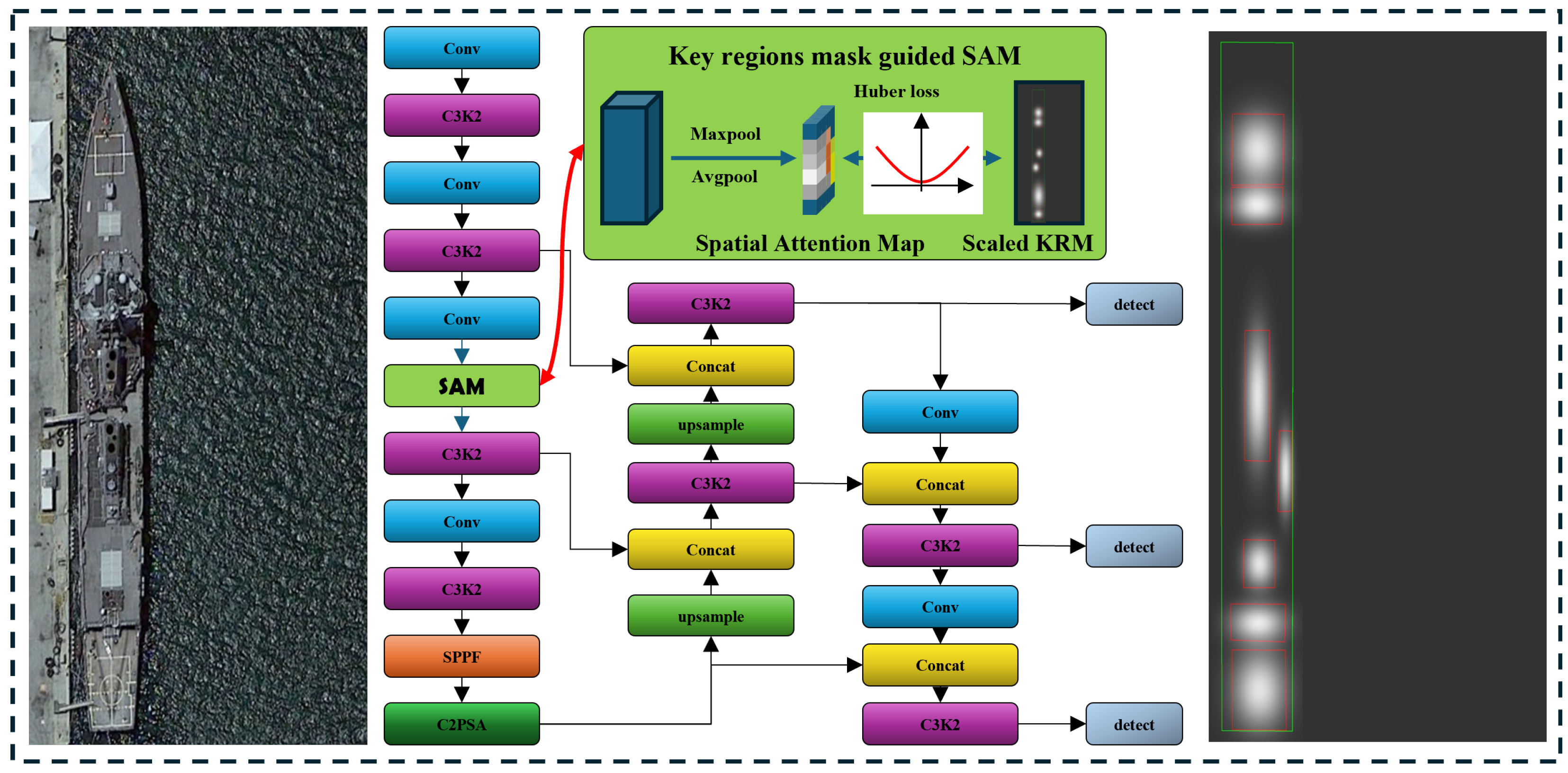
Figure 1.
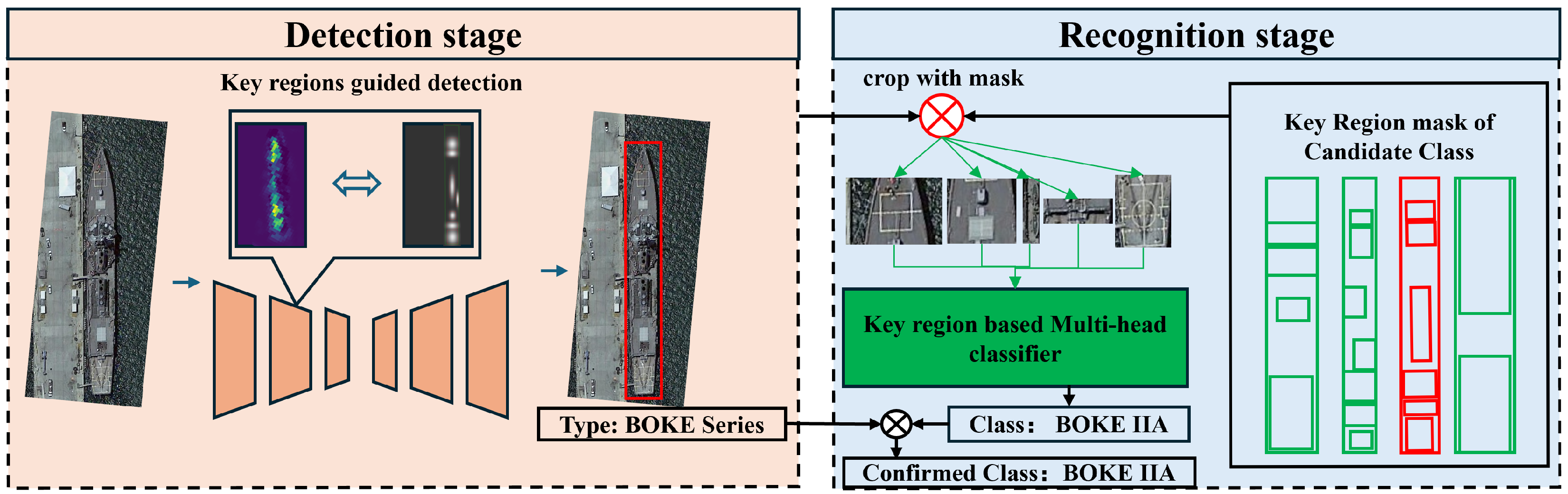
Framework of the proposed method, incorporating detection stage and recognition stage, which play the role of hypothesis and verification, respectively. With the key-region-guided detector, a bounding box with type is generated. Several groups of slices of key regions are generated with the bounding box and key region mask (KRM). Final results are decided by a multi-head classifier, the inputs of which are slices of key regions. In this figure, red and green boxes are bounding boxes.
Figure 1.
Framework of the proposed method, incorporating detection stage and recognition stage, which play the role of hypothesis and verification, respectively. With the key-region-guided detector, a bounding box with type is generated. Several groups of slices of key regions are generated with the bounding box and key region mask (KRM). Final results are decided by a multi-head classifier, the inputs of which are slices of key regions. In this figure, red and green boxes are bounding boxes.
Figure 2.
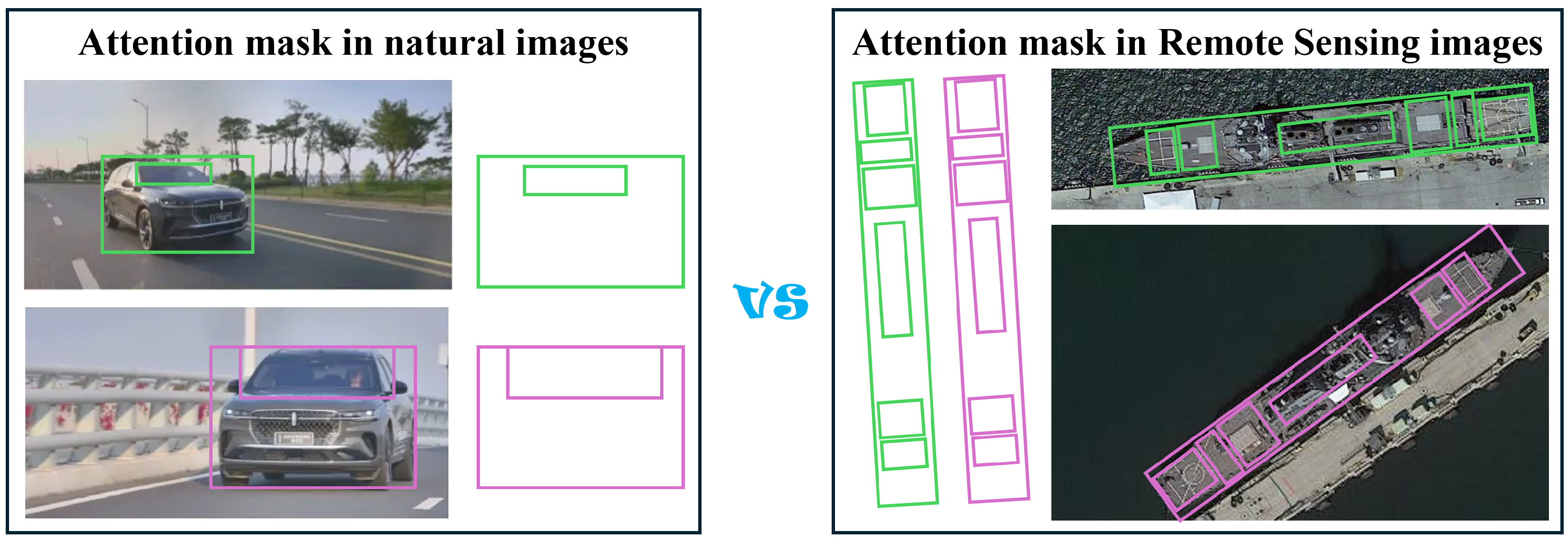
Differences between attention mask in natural images and RS images. In natural images, locations of key regions are not consistent in different viewing angles. The colorful boxes in this figure are bounding boxes of key regions.
Figure 2.
Differences between attention mask in natural images and RS images. In natural images, locations of key regions are not consistent in different viewing angles. The colorful boxes in this figure are bounding boxes of key regions.
Figure 3.
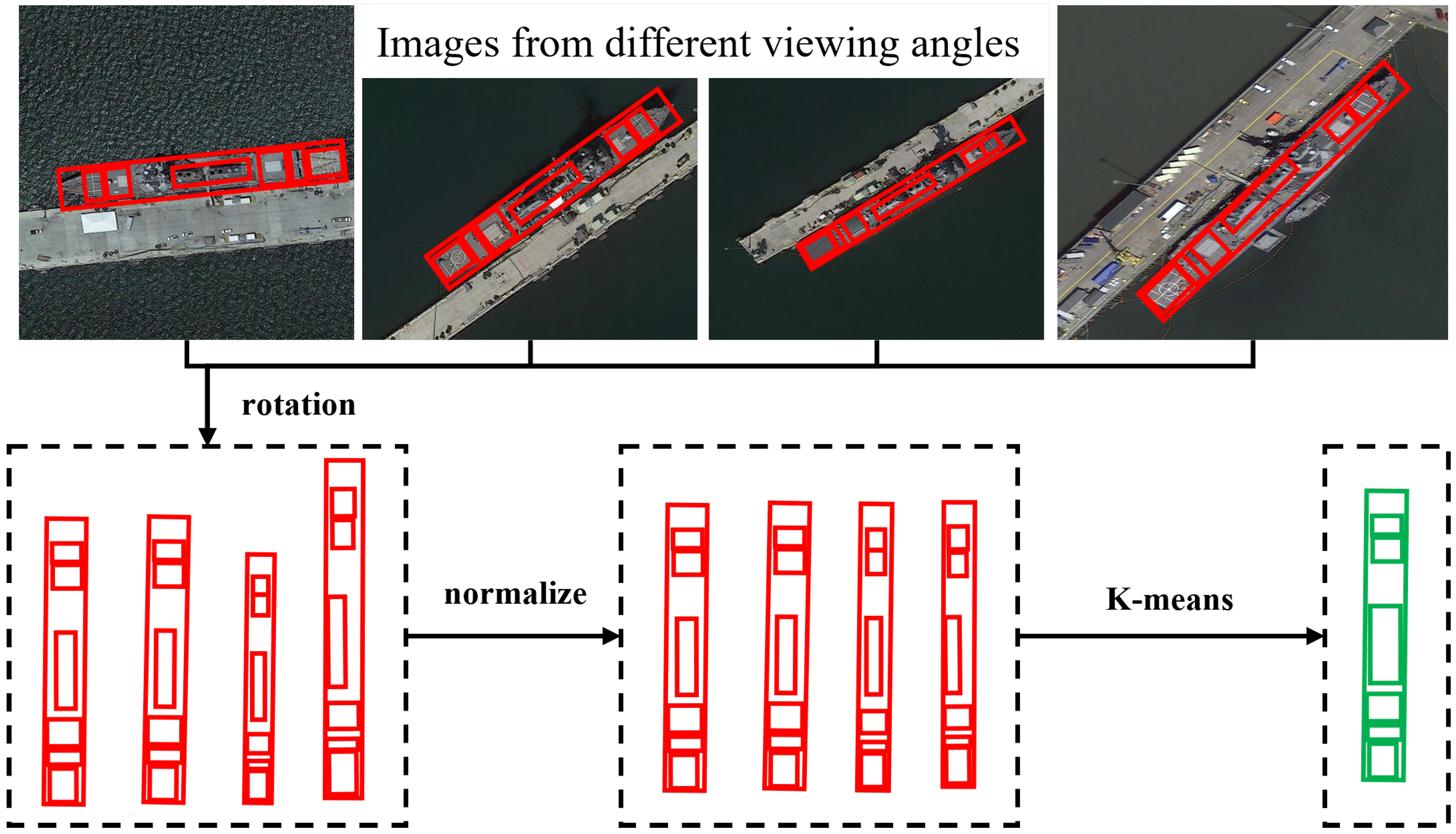
The generation of KRM of different ships via clustering diverse key regions (red boxes) from different viewing angles. Final key regions are suitable for different observation angles. Bounding boxes of the same class of ships from different viewpoints are uniformly rotated with the stern-to-bow direction as the y-axis and normalized to the same length. Accordingly, all key regions are resized and rotated using the same criteria to achieve mask alignment. Then, the normalized coordinates of key regions for each sample are recorded with the lower-left corner as the origin point. Finally, the KRM is (green box) generated with K-means, where .
Figure 3.
The generation of KRM of different ships via clustering diverse key regions (red boxes) from different viewing angles. Final key regions are suitable for different observation angles. Bounding boxes of the same class of ships from different viewpoints are uniformly rotated with the stern-to-bow direction as the y-axis and normalized to the same length. Accordingly, all key regions are resized and rotated using the same criteria to achieve mask alignment. Then, the normalized coordinates of key regions for each sample are recorded with the lower-left corner as the origin point. Finally, the KRM is (green box) generated with K-means, where .
Figure 4.
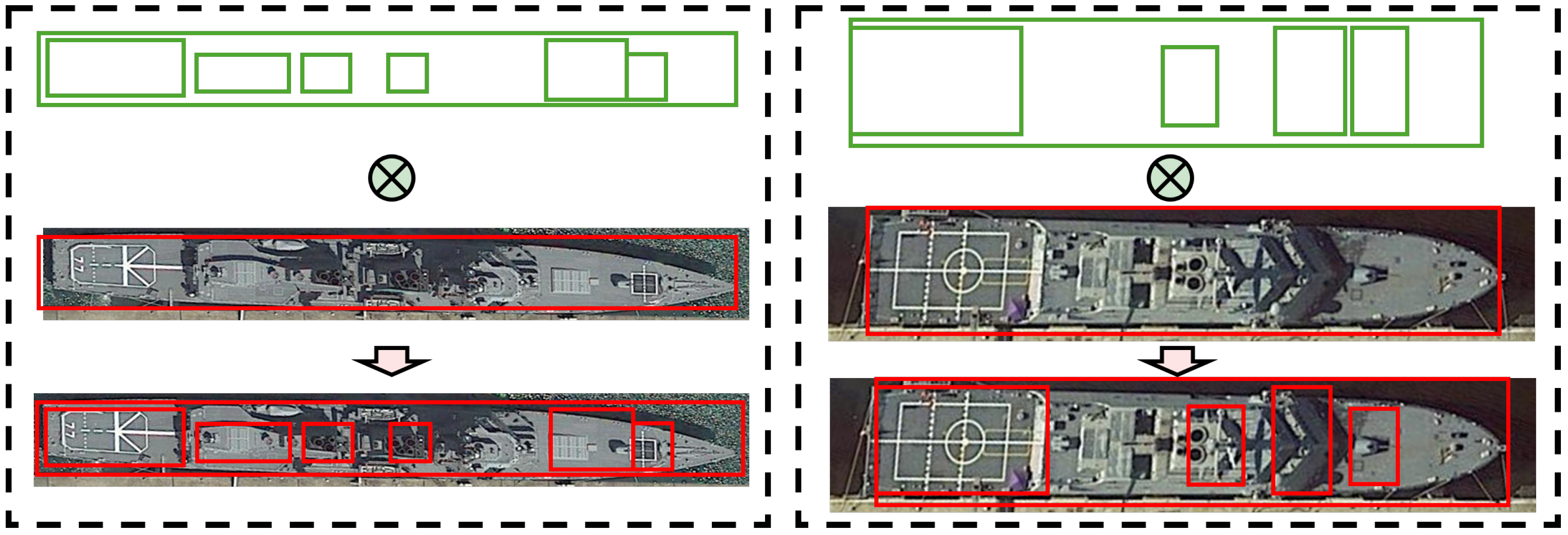
Attention masks are generated with bounding box (red boxes) and normalized template matrix (green boxes).
Figure 4.
Attention masks are generated with bounding box (red boxes) and normalized template matrix (green boxes).
Figure 5.
A spatial attention module (SAM) is embedded into the backbone network. The primary function of the detect module is to perform detection on feature maps of different resolutions. During the training phase, its output is constrained by an attention mask. Then in the inference, the module can focus on the key regions like human beings. Scaled KR-mask, generated by 1/8 down-sampling of the labeled mask, is adopted as ground truth of the spatial attention map. A Huber loss is formulated between the spatial attention map and scaled KRM.
Figure 5.
A spatial attention module (SAM) is embedded into the backbone network. The primary function of the detect module is to perform detection on feature maps of different resolutions. During the training phase, its output is constrained by an attention mask. Then in the inference, the module can focus on the key regions like human beings. Scaled KR-mask, generated by 1/8 down-sampling of the labeled mask, is adopted as ground truth of the spatial attention map. A Huber loss is formulated between the spatial attention map and scaled KRM.
Figure 6.
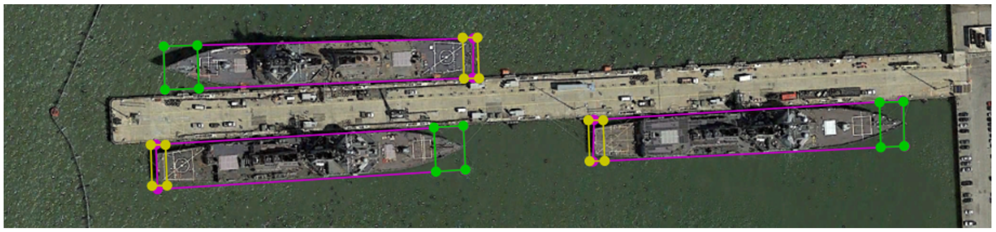
The stern, the bow and the ship are marked with a green, yellow and purple box respectively, to guide the mask generation method and target localization.
Figure 6.
The stern, the bow and the ship are marked with a green, yellow and purple box respectively, to guide the mask generation method and target localization.
Figure 7.
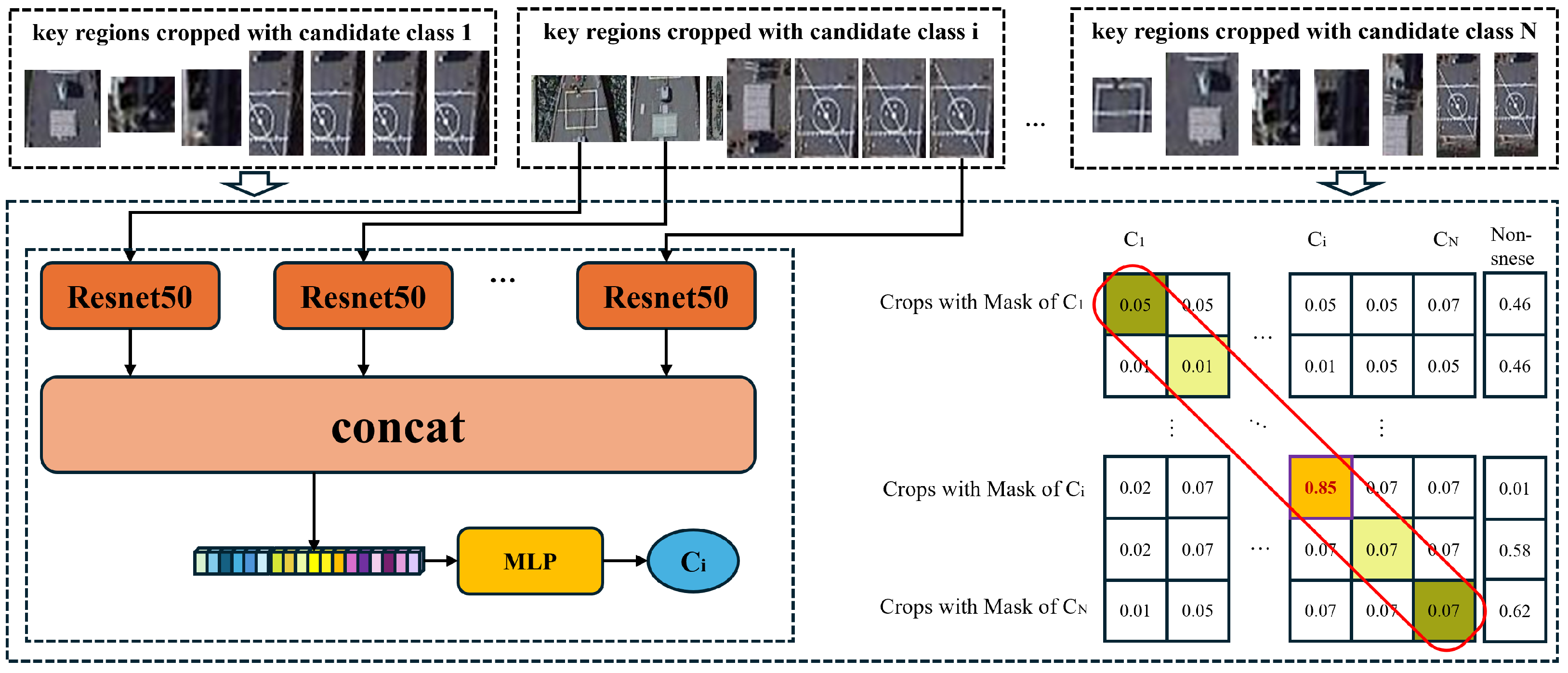
Framework of the proposed key regions-based MHC algorithm. Given N groups of key regions cropped with KRM of different candidate class, features are extracted with Resnet50. Features of key regions are concatenated in order and fed into a MLP layer, leading to a fixed-length (N + 1 classes) numerical vector. When all possible slices generated with the N masks are processed by the classifier, an N × (N + 1)-dimensional matrix is formed. The category corresponding to the maximum value along the diagonal of the first N × N submatrix (red box) represents the most probable ship class.
Figure 7.
Framework of the proposed key regions-based MHC algorithm. Given N groups of key regions cropped with KRM of different candidate class, features are extracted with Resnet50. Features of key regions are concatenated in order and fed into a MLP layer, leading to a fixed-length (N + 1 classes) numerical vector. When all possible slices generated with the N masks are processed by the classifier, an N × (N + 1)-dimensional matrix is formed. The category corresponding to the maximum value along the diagonal of the first N × N submatrix (red box) represents the most probable ship class.
Figure 8.
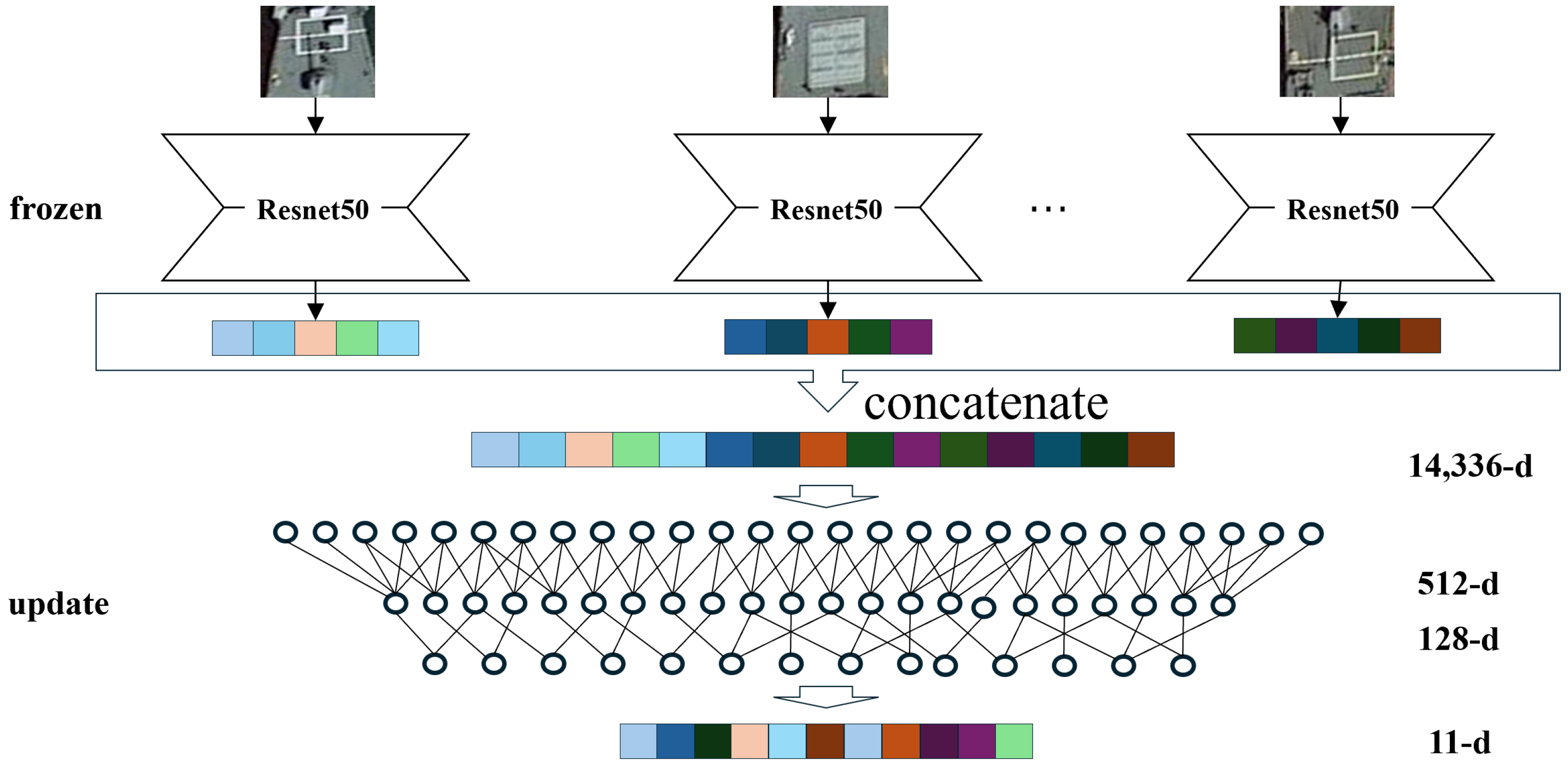
The entire training of MHC consists of two stages. The first stage is the training of the feature extractor ResNet50, which is frozen in the second stage. The second one is the training of the classification-aware layer in MHC.
Figure 8.
The entire training of MHC consists of two stages. The first stage is the training of the feature extractor ResNet50, which is frozen in the second stage. The second one is the training of the classification-aware layer in MHC.
Figure 9.
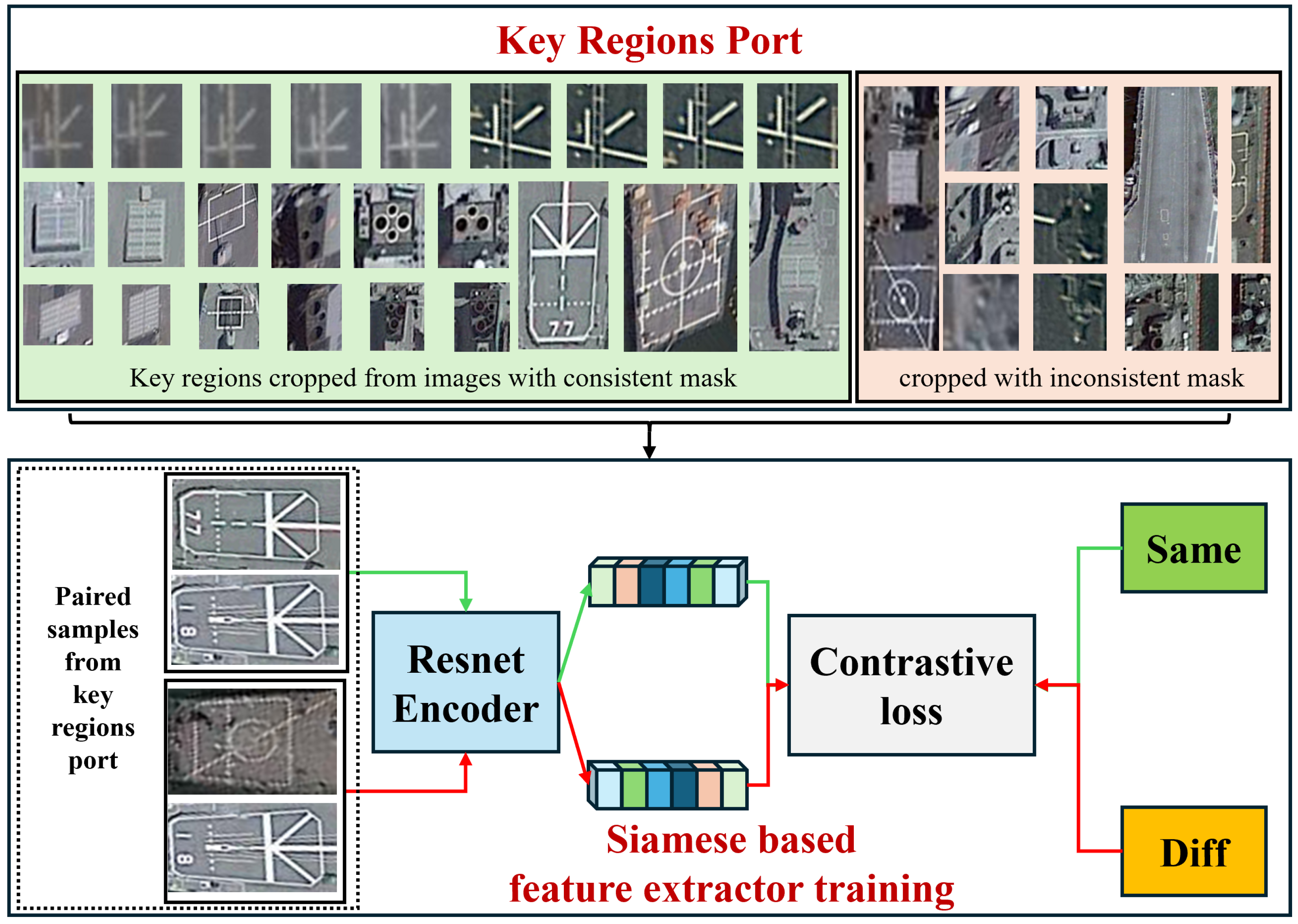
Generation schematic of the proposed contrastive learning-based feature extractor. Key regions port is composed of two parts, key regions cropped from images with consistent and inconsistent mask. With the same or different key regions from key region of the port paired, the siamese-network-based discriminator is trained with contrastive loss.
Figure 9.
Generation schematic of the proposed contrastive learning-based feature extractor. Key regions port is composed of two parts, key regions cropped from images with consistent and inconsistent mask. With the same or different key regions from key region of the port paired, the siamese-network-based discriminator is trained with contrastive loss.
Figure 10.
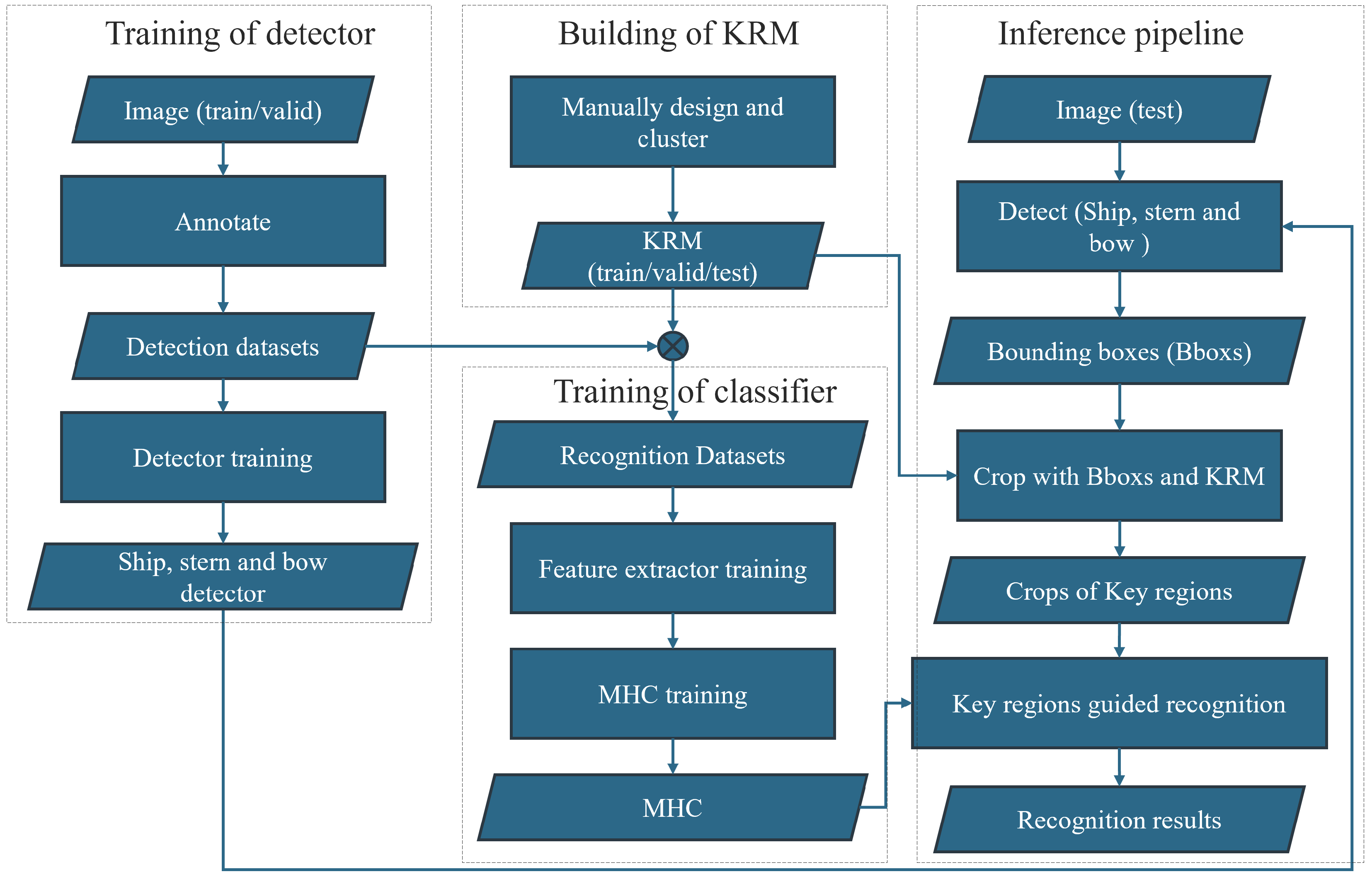
The block diagram of the proposed method. The overall framework consists of four parts, Building of the KRM, Training of the detector, Training of the classifier and the Inference pipeline.
Figure 10.
The block diagram of the proposed method. The overall framework consists of four parts, Building of the KRM, Training of the detector, Training of the classifier and the Inference pipeline.
Figure 11.
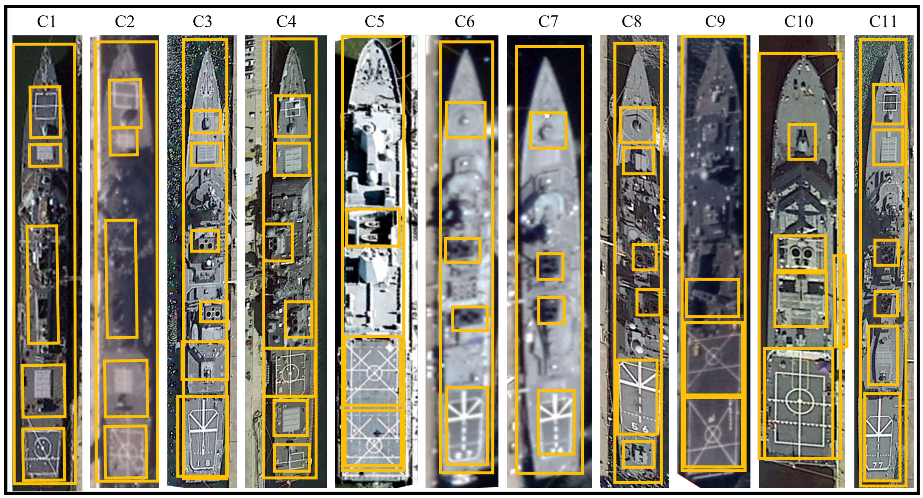
Samples in the DCL-11 dataset. The yellow bounding box is the key region mask for the proposed method.
Figure 11.
Samples in the DCL-11 dataset. The yellow bounding box is the key region mask for the proposed method.
Figure 12.
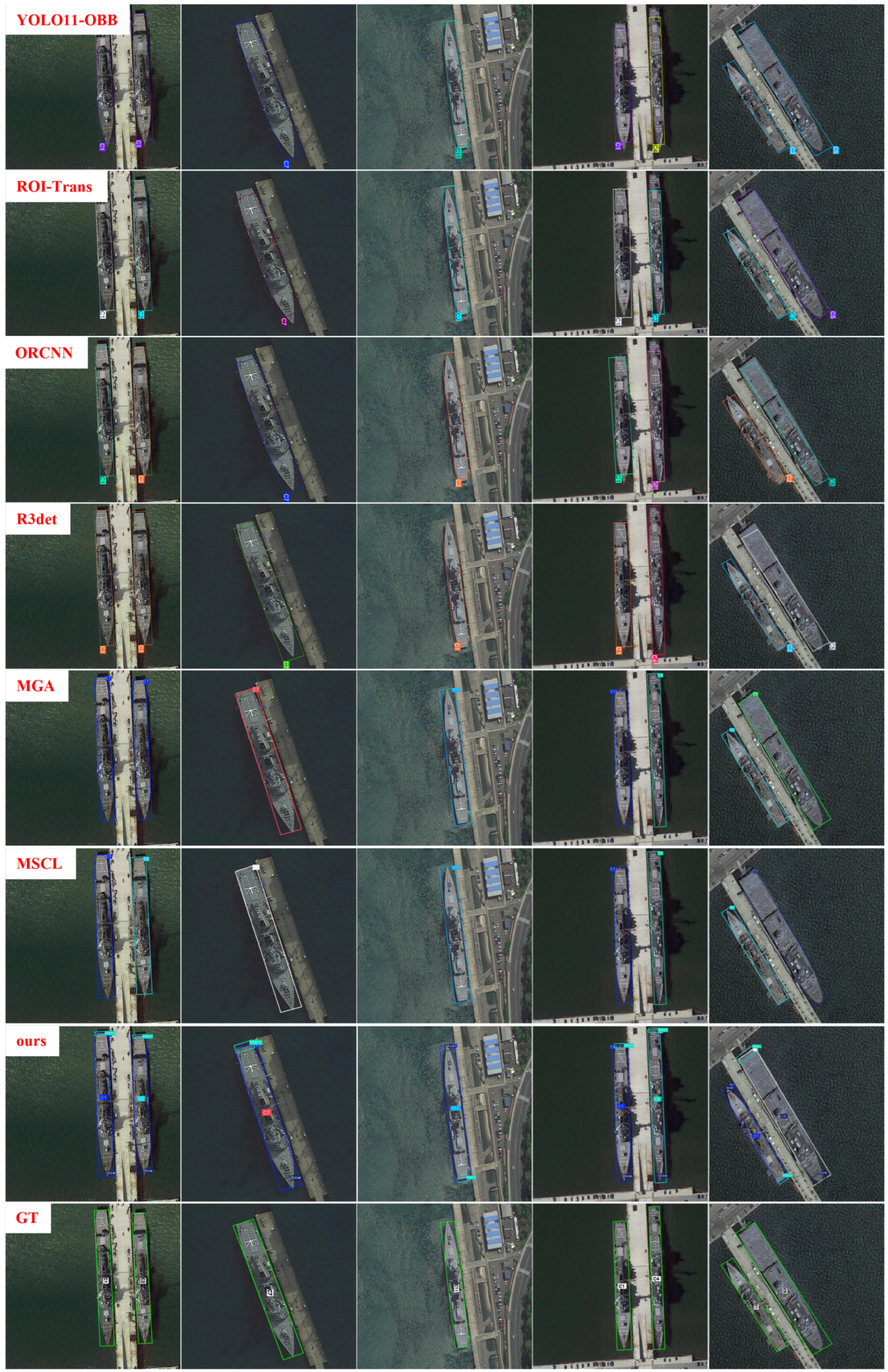
Detection and recognition results of SOTA and the proposed method. The ground truth are list in the last row. The colorful boxes are bounding box of ships.
Figure 12.
Detection and recognition results of SOTA and the proposed method. The ground truth are list in the last row. The colorful boxes are bounding box of ships.
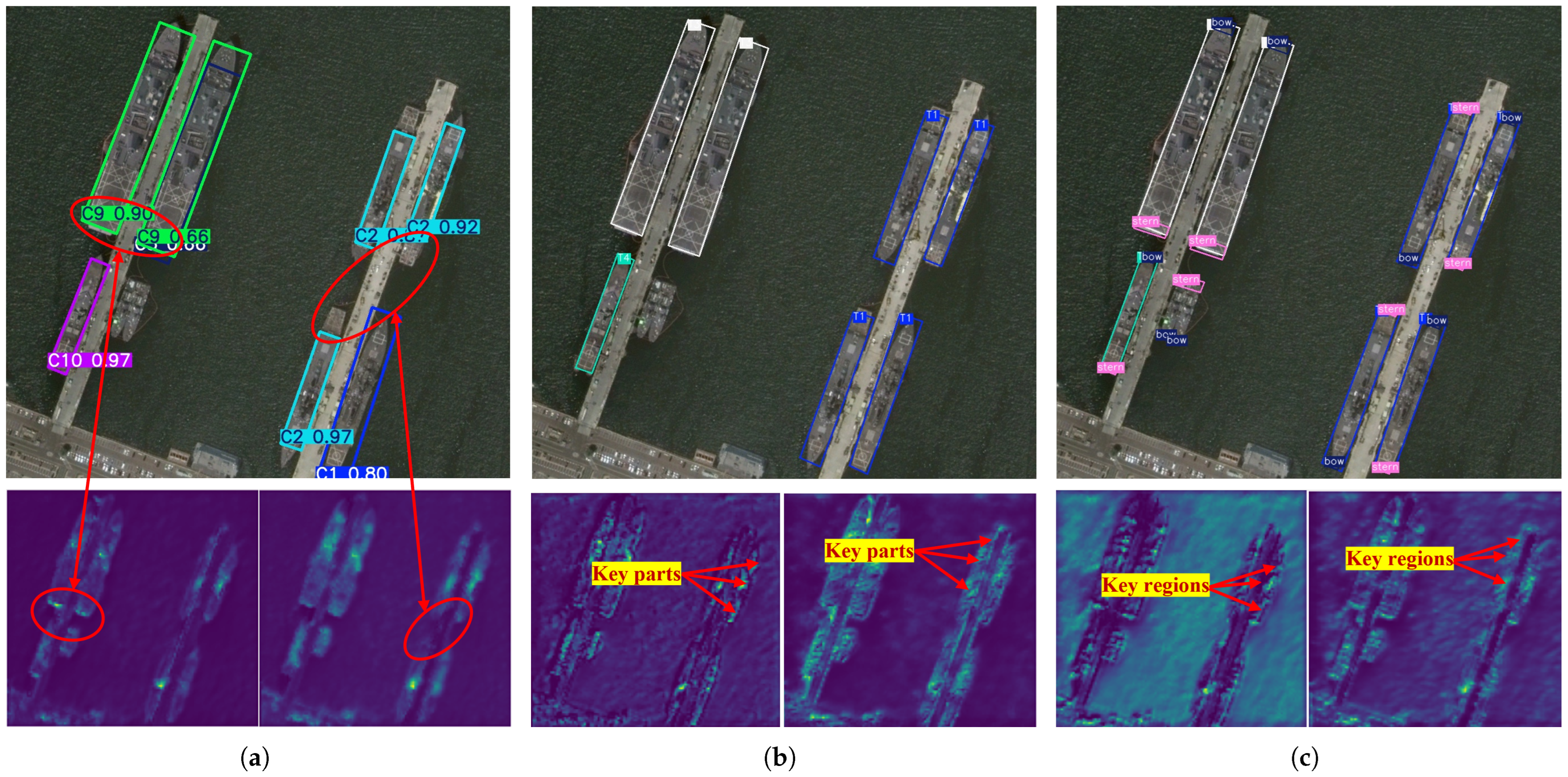
Figure 13.
Comparative visualization results and feature visualization heatmaps before and after incorporating the KR-guided-attention module and the part-to-whole (PTW) relation regulation mechanism. (a) Detection results of YOLO11-OBB and visualized feature map (C3k2). (b) Detection results of YOLO11-OBB with the KR-guided-attention module and visualized feature map (C3k2). (c) Detection results of YOLO11-OBB with the KR-guided-attention module and and the part-to-whole relation regulation mechanism, followed with visualized feature map (C3k2).
Figure 13.
Comparative visualization results and feature visualization heatmaps before and after incorporating the KR-guided-attention module and the part-to-whole (PTW) relation regulation mechanism. (a) Detection results of YOLO11-OBB and visualized feature map (C3k2). (b) Detection results of YOLO11-OBB with the KR-guided-attention module and visualized feature map (C3k2). (c) Detection results of YOLO11-OBB with the KR-guided-attention module and and the part-to-whole relation regulation mechanism, followed with visualized feature map (C3k2).
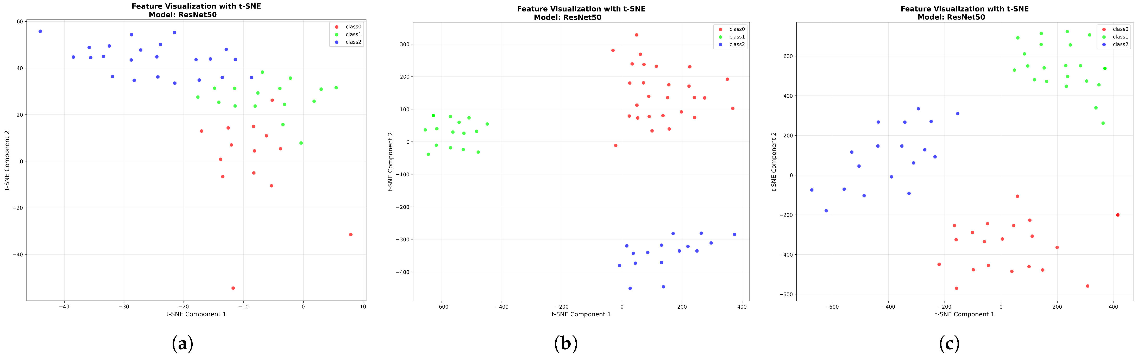
Figure 14.
(a) The visualized dimensionality-reduced feature of whole ship extracted with trained ResNet50, where class0, class1, and class2 correspond to the boke-II, boke-IIA, and Kongo-class, respectively. (b) The visualized dimensionality-reduced feature of helicopter decks from the three ship classes with trained ResNet50, where class0, class1, and class2 correspond to the helicopter decks of the boke-II, boke-IIA, and Kongo-class, respectively. (c) The visualized dimensionality-reduced concatenated key-region features from the three ship classes using ResNet50, where class0, class1, and class2 represent the key-region combinations of the boke-II, boke-IIA, and Kongo-class, respectively.
Figure 14.
(a) The visualized dimensionality-reduced feature of whole ship extracted with trained ResNet50, where class0, class1, and class2 correspond to the boke-II, boke-IIA, and Kongo-class, respectively. (b) The visualized dimensionality-reduced feature of helicopter decks from the three ship classes with trained ResNet50, where class0, class1, and class2 correspond to the helicopter decks of the boke-II, boke-IIA, and Kongo-class, respectively. (c) The visualized dimensionality-reduced concatenated key-region features from the three ship classes using ResNet50, where class0, class1, and class2 represent the key-region combinations of the boke-II, boke-IIA, and Kongo-class, respectively.
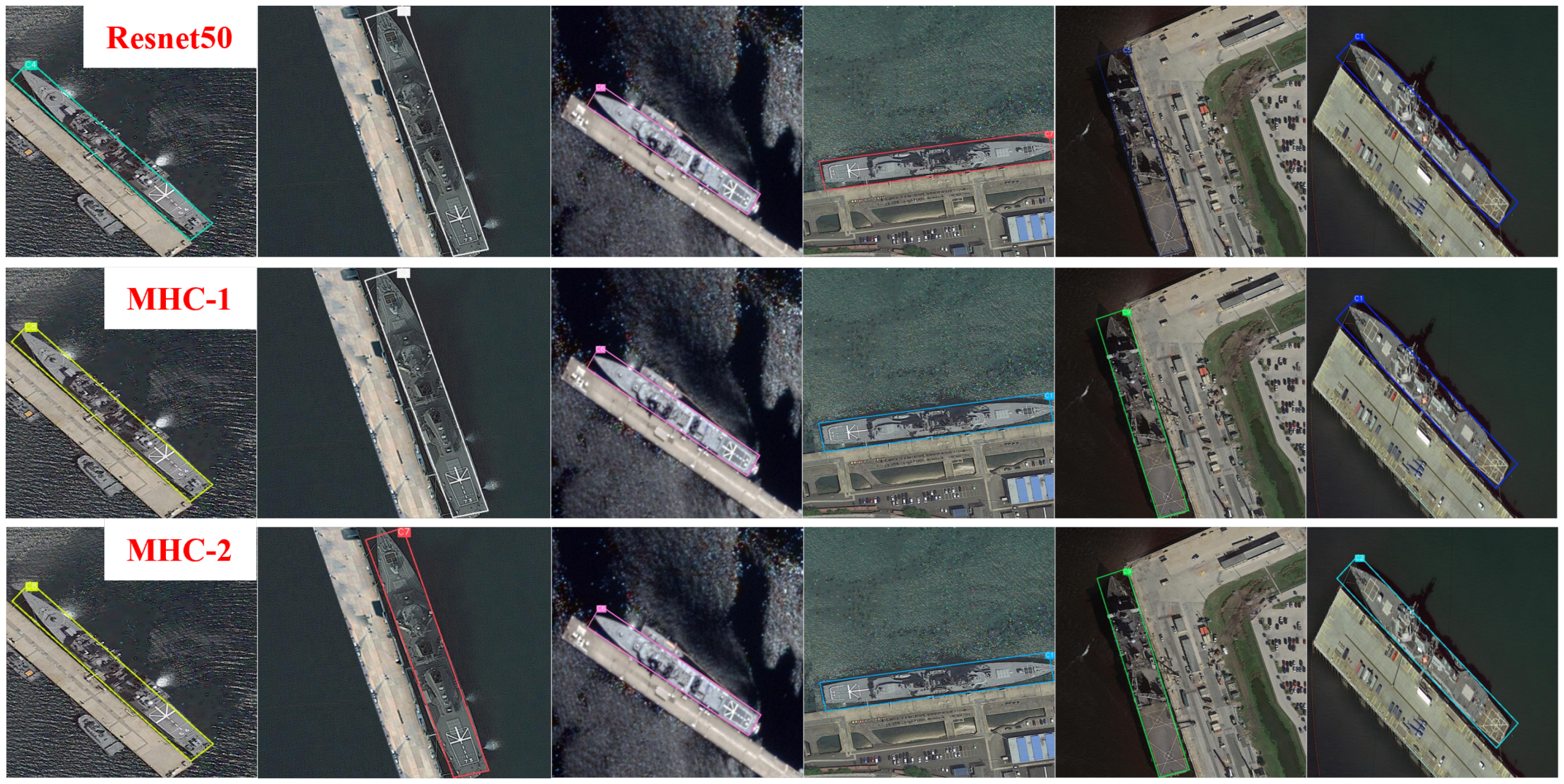
Figure 15.
Classification result of module with Resnet50, MHC-1 and MHC-2.
Figure 15.
Classification result of module with Resnet50, MHC-1 and MHC-2.
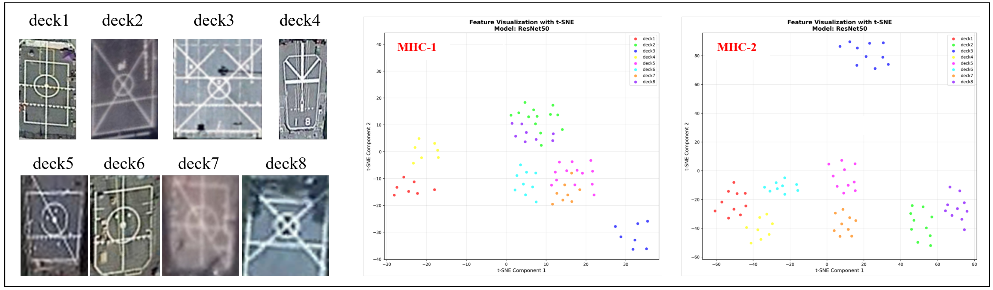
Figure 16.
Eight kinds of classical helicopter deck and their feature in T-SNE with MHC-1 and MHC-2.
Figure 16.
Eight kinds of classical helicopter deck and their feature in T-SNE with MHC-1 and MHC-2.
Figure 17.
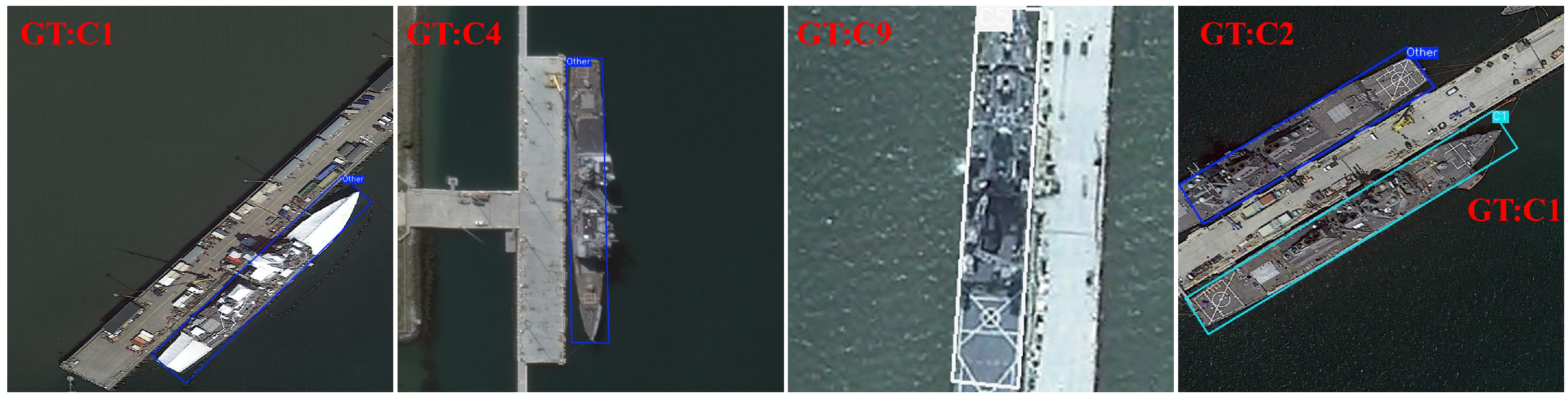
Fail cases caused by incomplete boxes and occlusion. GT indicates ground truth.
Figure 17.
Fail cases caused by incomplete boxes and occlusion. GT indicates ground truth.
Table 1.
The composition of the dataset DCL-11.
Table 1.
The composition of the dataset DCL-11.
| Ship Type | Ship Class | Count | Total |
|---|
| Spruance Series | Ticonderoga | 701 | 904 |
| Asagiri | 203 |
| Burke Series | Murasame | 202 | 2079 |
| Arleigh Burke-II | 550 |
| Arleigh Burke-IIA | 510 |
| Kongo | 275 |
| Akizuki | 286 |
| Atago | 256 |
| Littoral Combat Ship Series | Independence | 655 | 655 |
| Dock Landing Ship Series | San Antonio | 876 | 1608 |
| Whitby Island | 732 |
Table 2.
MAP of algorithms with different weighting setting about and with PTW and MHC-2.
Table 2.
MAP of algorithms with different weighting setting about and with PTW and MHC-2.
| | Case 1 | Case 2 | Case 3 | Case 4 | Case 5 | Case 6 | Case 7 | Case 8 |
|---|
| 1.000 | 0.950 | 0.925 | 0.900 | 0.875 | 0.850 | 0.825 | 0.800 |
| 0.050 | 0.050 | 0.075 | 0.100 | 0.125 | 0.150 | 0.175 | 0.200 |
| MAP | 93.71 | 93.79 | 93.96 | 94.12 | 94.49 | 94.31 | 93.69 | 93.12 |
Table 3.
MAP of the proposed and SOTA detection methods.
Table 3.
MAP of the proposed and SOTA detection methods.
| Class | RoITrans | R3Det | O-RCNN | YOLOv11 | MGANet | MSCL-Net | KRGY-MHC |
|---|
| C1 | 93.53 | 93.33 | 93.46 | 93.22 | 94.5 | 94.36 | 96.53 |
| C2 | 93.71 | 94.29 | 93.17 | 93.19 | 94.88 | 94.21 | 96.19 |
| C3 | 91.25 | 91.39 | 91.13 | 91.84 | 92.26 | 92.12 | 93.28 |
| C4 | 93.21 | 93.18 | 93.32 | 93.47 | 94.24 | 94.18 | 96.21 |
| C5 | 90.82 | 90.92 | 91.86 | 90.75 | 91.81 | 91.95 | 93.86 |
| C6 | 89.76 | 91.16 | 89.98 | 91.22 | 92.30 | 92.16 | 91.08 |
| C7 | 91.31 | 91.29 | 88.42 | 91.32 | 92.36 | 92.22 | 91.89 |
| C8 | 93.38 | 93.45 | 93.23 | 93.09 | 94.31 | 94.42 | 96.32 |
| C9 | 90.72 | 90.8 | 90.64 | 90.91 | 91.78 | 91.85 | 93.71 |
| C10 | 93.78 | 93.92 | 93.25 | 93.37 | 94.09 | 94.21 | 96.08 |
| C11 | 91.63 | 90.75 | 91.76 | 90.63 | 92.18 | 91.93 | 94.22 |
Table 4.
MAP of six kind of algorithms.
Table 4.
MAP of six kind of algorithms.
| | Case1 | Case2 | Case3 | Case4 | Case5 | Case6 |
|---|
| YOLO-OBB | ✓ | ✓ | ✓ | ✓ | ✓ | ✓ |
| KRGY | | ✓ | | ✓ | ✓ | ✓ |
| PTW | | | ✓ | ✓ | ✓ | ✓ |
| Resnet50 | | | | ✓ | | |
| MHC-1 | | | | | ✓ | |
| MHC-2 | | ✓ | ✓ | | | ✓ |
| MAP | 92.28 | 93.65 | 93.71 | 93.82 | 94.28 | 94.49 |
Table 5.
The silhouette score of three different inputs in
Figure 14.
Table 5.
The silhouette score of three different inputs in
Figure 14.
| | Class0 | Class1 | Class2 |
|---|
| Feature of whole ship | 0.062 | 0.377 | 0.316 |
| Feature of key regions | 0.665 | 0.669 | 0.637 |
| Feature of grouped key regions | 0.480 | 0.723 | 0.436 |
Table 6.
The silhouette score of 8 kinds of classical helicopter decks with MHC-1 and MHC-2 in
Figure 16.
Table 6.
The silhouette score of 8 kinds of classical helicopter decks with MHC-1 and MHC-2 in
Figure 16.
| | Deck1 | Deck2 | Deck3 | Deck4 | Deck5 | Deck6 | Deck7 | Deck8 |
|---|
| MHC-1 | 0.529 | 0.096 | 0.713 | 0.538 | 0.094 | 0.517 | 0.318 | 0.220 |
| MHC-2 | 0.501 | 0.495 | 0.808 | 0.569 | 0.567 | 0.624 | 0.651 | 0.559 |
Table 7.
Impact on the recognition rate of a small amount of positioning deviation of bounding box extraction in the first stage.
Table 7.
Impact on the recognition rate of a small amount of positioning deviation of bounding box extraction in the first stage.
| Case | Case1 | Case2 | Case3 | Case4 | Case5 |
|---|
| Positioning Deviation | | | | | |
| Recognition Rate | | | | | |




 ,
,