


Highlights
What are the main findings?
- An AutoML-based daily model integrating FLUXNET-CH4, ERA5-Land, MODIS, and HWSD data accurately predicts daily rice paddy CH4 fluxes (CC = 0.897 for 5-fold and CC = 0.819 for leave-one-year-out cross-validation).
- Variable importance shifts with temporal resolution: soil temperature dominates daily emissions (~50% contribution), whereas the hourly model exhibits a more multivariate structure, where vegetation status (NDVI) and soil moisture become more influential in regulating diurnal emission sensitivities and short-term dynamics.
What are the implications of the main findings?
- The 500 m daily gridded CH4 maps, validated by robust temporal generalization (LOYO), support the refinement of national inventories and the implementation of spatially targeted mitigation strategies, such as precise water management timing.
- The multi-resolution framework provides a quantitative basis for selecting temporal resolution in operational emission monitoring, balancing mapping efficiency with process-level interpretability.
Abstract
Agriculture is a major global source of methane (CH4), and accurate emission estimates are essential for refining national greenhouse gas inventories and supporting climate-resilient policies. This study develops a high-resolution estimation framework for CH4 emissions from Korean rice paddies by integrating multi-source datasets, including Moderate Resolution Imaging Spectroradiometer (MODIS) vegetation indices, European Centre for Medium-Range Weather Forecasts (ECMWF) Reanalysis Version 5 (ERA5)-Land meteorological variables, and Harmonized World Soil Database (HWSD) soil properties. Using CH4 flux observations from four global rice ecosystems (Italy, Japan, South Korea, and USA), we constructed parallel daily and hourly machine learning models using an automated machine learning (AutoML) framework to compare their performance and process-level interpretability. The daily model demonstrated high predictive accuracy with correlation coefficients (CC) of 0.897 in 5-fold cross-validation and 0.819 in Leave-One-Year-Out (LOYO) cross-validation. Shapley Additive Explanations (SHAP) analysis revealed that while soil temperature is the dominant predictor for daily emissions (explaining ~50% of the variance), variable importance shifts significantly at finer resolutions. The hourly model exhibited a more complex multivariate structure. In this high-resolution context, although Normalized Difference Vegetation Index (NDVI) remains constant diurnally, its importance strengthens as a critical regulator of emission sensitivity, interacting with hourly meteorological fluctuations to capture short-term dynamics. The resulting 500 m daily gridded maps provide a robust foundation for national inventory refinement and spatially targeted mitigation planning. Our findings suggest that while the daily model offers optimal computational efficiency for long-term monitoring, the hourly model is superior for mechanistic understanding and detecting episodic emission events. This multi-resolution framework establishes an empirical basis for selecting appropriate temporal scales in operational greenhouse gas monitoring systems.
1. Introduction
Rice paddies are a major anthropogenic source of global methane (CH4) emissions, accounting for a substantial fraction of the agricultural sector’s greenhouse gas footprint, particularly in Asia. The flooded conditions of paddy fields create anaerobic environments that promote the activity of methanogenic microorganisms, leading to significant methane release during the growing season. Approximately 10% of global methane emissions are estimated to originate from rice cultivation [1,2]. These emissions exhibit pronounced temporal and spatial heterogeneity, driven by seasonally concentrated cropping cycles and irrigation-based water management.
A defining challenge in studying rice paddy methane emissions is their extreme spatiotemporal variability. Emission rates fluctuate in response to climatic conditions, soil properties, water management practices, and rice phenological stages [3,4]. This variability complicates accurate quantification at regional and national scales, as point-based measurements at individual sites often fail to represent the diverse environmental and management conditions across larger areas. Spatial heterogeneity arises from regional differences in environmental factors, while temporal variability occurs across multiple scales—ranging from diurnal fluctuations driven by temperature and plant physiology to seasonal and interannual patterns linked to cultivation cycles and meteorology [5,6,7,8].
Despite the importance of rice cultivation in South Korea, studies on nationwide methane emissions remain limited in both spatial and temporal resolution [9,10]. Previous research has primarily relied on point-based observations or linear regression approaches. However, these methods face several limitations: (1) their coarse temporal resolution (often monthly or annual) fails to capture short-term dynamics such as flooding-to-drainage transitions, rapid soil temperature changes, and vegetation development; (2) estimates based on administrative statistics or static emission factors cannot account for fine-scale, field-level management differences [10,11]; and (3) they struggle to model the nonlinear, interacting processes governing methane production and transport. As a result, a clear gap remains in South Korea in nationwide methane emission estimates at sub-kilometer spatial and daily temporal resolutions that can capture nonlinear driver interactions and short-term dynamics.
Recent advances in high-resolution spatial datasets—including vegetation indices from the Moderate Resolution Imaging Spectroradiometer (MODIS), meteorological and soil data from European Centre for Medium-Range Weather Forecasts (ECMWF) Reanalysis Version 5 (ERA5)-Land, and soil information from the Harmonized World Soil Database (HWSD)—have enabled the development of data-driven models that integrate multi-source information. However, many of these studies remain constrained by coarse spatial or temporal resolutions, or focus on site-scale applications, limiting their ability to resolve daily variability and field-level emission hotspots [5,6,7,8]. Furthermore, Automated Machine Learning (AutoML) frameworks now allow for efficient nonlinear modeling by automating model selection and hyperparameter optimization. Despite the availability of these tools, no previous study has integrated these datasets to reconstruct rice paddy methane emissions in South Korea at both high spatial and daily temporal resolutions. Furthermore, the impact of temporal resolution (hourly vs. daily) on identifying dominant drivers and variable importance has not yet been systematically evaluated.
In this study, we develop the first nationwide methane emission maps for South Korean rice paddies at 500 m spatial and daily temporal resolution. We achieve this by integrating ground-based flux measurements (FLUXNET-CH4), meteorological reanalysis (ERA5-Land), satellite remote sensing (MODIS), and soil properties (HWSD) within an automated machine learning framework. We construct parallel daily and hourly models using identical data sources and validation schemes to assess how temporal resolution influences model performance and variable importance.
Our findings establish a framework for selecting appropriate temporal scales based on specific application goals. By integrating multi-source data, this study extends previous research on spatiotemporal emission dynamics [12] and regional-scale estimates [6]. We demonstrate that while soil temperature dominates daily variability, the hourly model reveals a multivariate structure where vegetation status and soil moisture act as critical regulators of diurnal sensitivity. These high-resolution maps provide a valuable dataset to complement traditional emission-factor approaches, supporting the improvement of national greenhouse gas inventories and the design of effective water-management mitigation strategies.
2. Materials and Methods
2.1. Study Area
This study encompasses the entire rice cultivation area of South Korea. Rice paddies, which constitute approximately 16% of the national land area, are predominantly distributed across Jeollanam-do, Jeollabuk-do, Chungcheongnam-do, and Gyeonggi-do. These regions feature hot, humid summers and extensive irrigation infrastructure, providing optimal conditions for rice production. However, the characteristic flooding and organic matter inputs also foster anaerobic environments conducive to CH4 production, making these areas significant sources of agricultural emissions. CH4 flux is primarily concentrated during the irrigation season in South Korea, typically from July to October (from transplanting to harvest), and varies significantly with water management, soil properties, organic amendments, and climatic factors. Here, we estimated daily CH4 emissions and quantified their spatiotemporal dynamics at a national scale using satellite-derived datasets. To ensure high-precision analysis, the study domain was restricted to rice paddies by masking the Farm Map land cover dataset from the National Geospatial Information Platform. This approach minimizes potential uncertainties from non-agricultural land or other crop types, allowing for a focused assessment of methane-active paddy fields. All environmental predictors used in this study are provided at a native spatial resolution of 500 m. Accordingly, flux tower observations were assigned to the corresponding 500 m grid cell containing each tower location.
2.2. Research Framework and Workflow
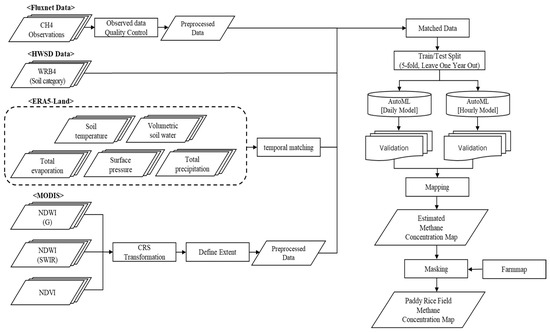
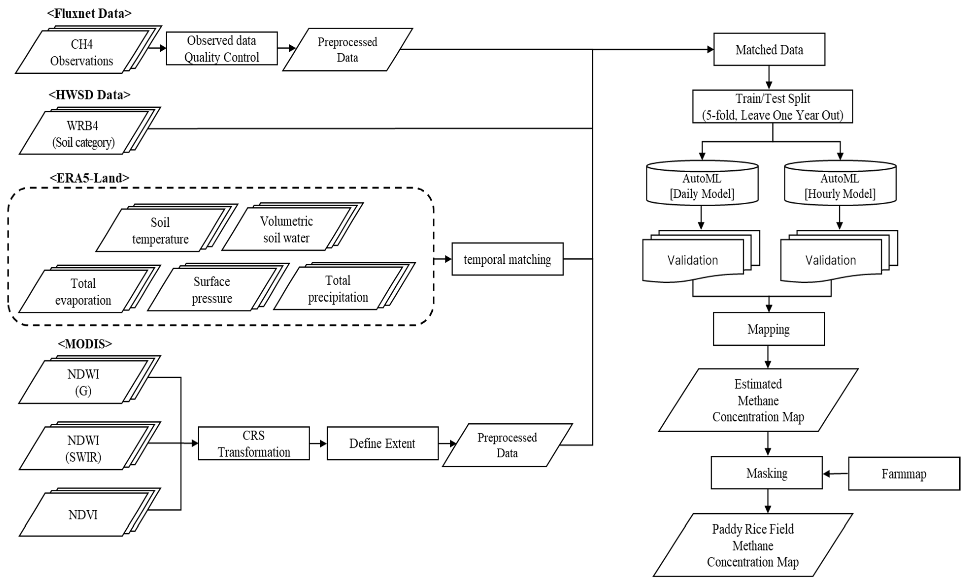
A systematic workflow was established to develop high-resolution CH4 emission maps for rice paddies by integrating in situ flux observations with multi-source satellite and environmental datasets (Figure 1). The research process was conducted in four primary stages:
Figure 1.
Methodological framework and workflow for national-scale rice paddy CH4 emission mapping in South Korea. The workflow includes (i) collection of CH4 flux observations and multi-source environmental predictors (MODIS vegetation indices, ERA5-Land meteorological variables, and HWSD soil category), (ii) quality control and preprocessing (coordinate transformation, spatial extent definition, and resampling), (iii) temporal matching between flux observations and predictor variables, and (iv) model training and validation using AutoML for both daily and hourly emission estimation (5-fold cross-validation and leave-one-year-out validation). The trained models were applied to generate gridded methane emission maps, which were subsequently masked using the national rice paddy farm map to produce rice paddy–specific CH4 emission products.
- Data Preprocessing and Quality Control: Methane flux measurements were subjected to rigorous quality control to eliminate outliers and filter out abnormal temporal variability.
- Data Integration and Harmonization: MODIS-derived vegetation indices, ERA5-Land meteorological variables, and HWSD soil properties were preprocessed and harmonized to a consistent 500 m spatial resolution. These environmental drivers were then spatiotemporally collocated with the flux observations to construct a robust training dataset.
- Model Development and Validation: Daily and hourly methane prediction models were developed using an AutoML framework. The models’ predictive accuracy and generalization performance were evaluated using both 5-fold cross-validation and Leave-One-Year-Out (LOYO) validation.
- Mapping and Masking: Finally, the trained models were applied to national-scale gridded input data to generate 500 m methane emission maps. A high-resolution rice paddy mask was applied to the results to strictly restrict predictions to active cultivation areas.
- Implementation details: All analyses were implemented in Python (v3.9.21) using FLAML (v2.3.5) and scikit-learn (v1.4.2) libraries.
2.3. Datasets
The model input variables were selected to comprehensively represent the meteorological conditions, vegetation status, surface water levels, and soil characteristics that drive methane production in rice paddies. To achieve this, we integrated MODIS-derived vegetation indices, meteorological and soil reanalysis data from ERA5-Land, soil properties from the HWSD, and ground-based methane flux observations from FLUXNET-CH4. This multi-source integration enables a spatially explicit representation of methane emission characteristics across the diverse climatic and pedological (soil) conditions found throughout South Korea.
2.3.1. FLUXNET In situ Data
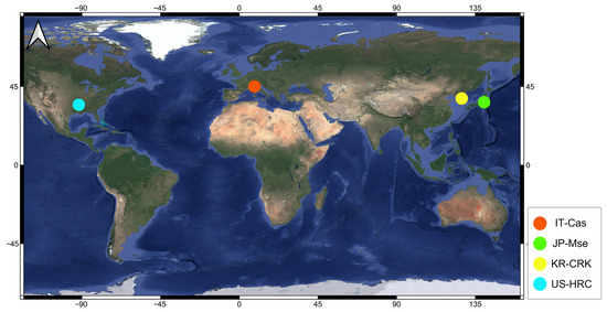
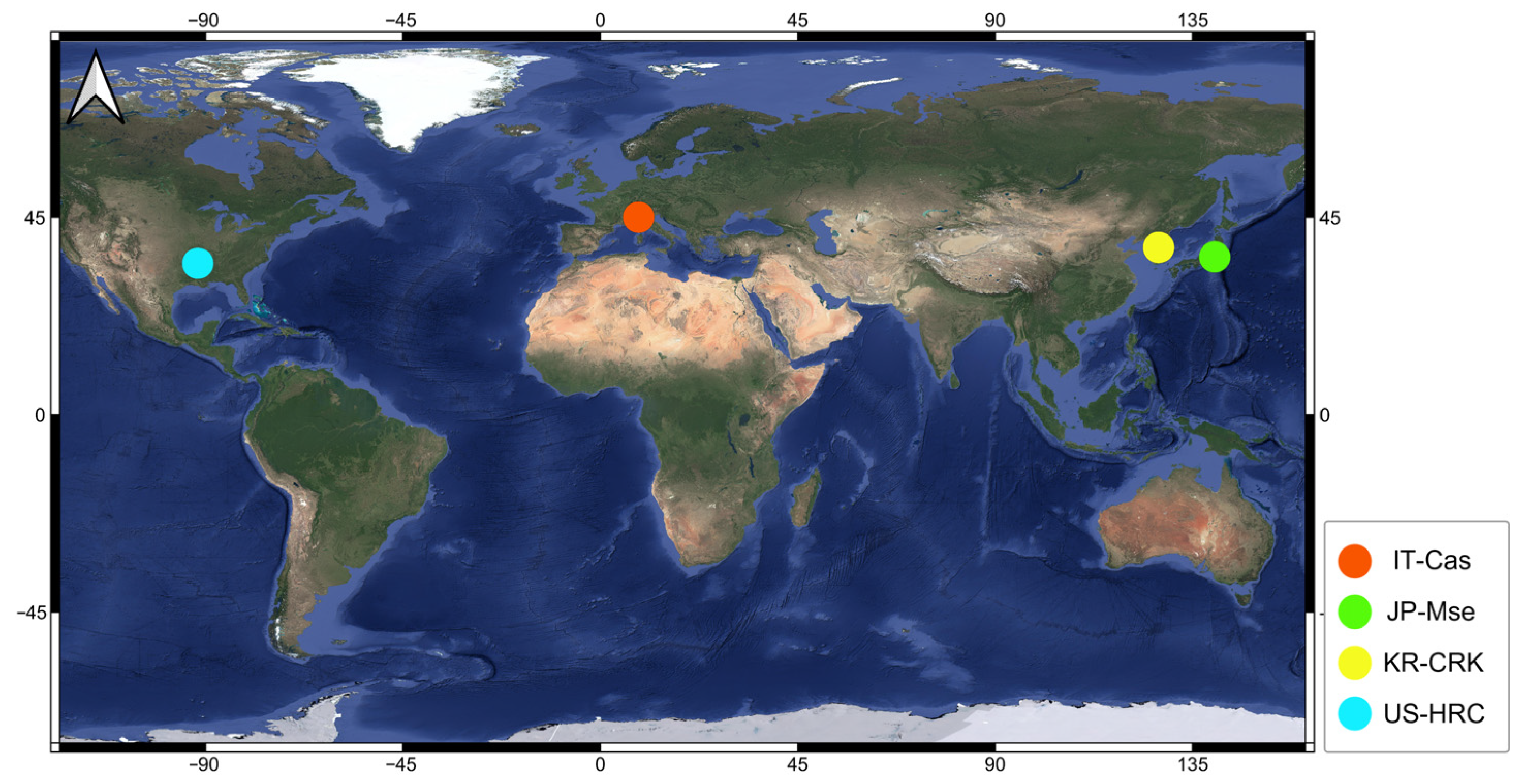
Methane flux data were sourced from the FLUXNET-CH4 Community Product, which provides standardized, quality-controlled CH4 measurements derived from a global network of eddy covariance towers [13,14]. To ensure the model’s robustness, we utilized observations from four rice paddy sites representing a variety of climatic conditions: IT-Cas (Castellaro, Mantua, Italy), JP-Mse (Mase, Tsukuba, Japan), KR-CRK (Cheorwon, Gangwon, South Korea), and US-HRC (Humnoke Rice Site, Lonoke County, AR, USA) (Table 1; Figure 2).
Table 1.
Summary of geographic locations and observation periods for the four FLUXNET-CH4 rice paddy sites used in this study.
Figure 2.
Geographic distribution of the four FLUXNET-CH4 rice paddy eddy covariance sites used in this study. The sites include IT-Cas (Italy), JP-Mse (Japan), KR-CRK (South Korea), and US-HRC (United States). These sites were used to provide CH4 flux observations spanning diverse climatic and environmental conditions for model training and validation.
Data spanning 2009–2018 were extracted to construct a decade-long dataset that captures both seasonal dynamics and interannual variability. This geographic and climatic diversity is instrumental in developing a generalized model that is not localized to a single site, making it suitable for national-scale methane mapping in South Korea. Following rigorous quality control, the final dataset comprised 1940 validated daily observations.
Extending methane flux observations to broader Asian rice systems would be valuable; however, long-term, consistently quality-controlled public datasets across China, India, and Southeast Asia remain limited. Moreover, field studies from tropical rice systems (e.g., the Philippines) report substantial diurnal and seasonal variability in CH4 fluxes, suggesting that indiscriminate pooling of heterogeneous datasets may increase uncertainty in model integration and interpretation [15,16].
International flux sites were included not to directly transfer site-specific emission magnitudes to South Korea, but to broaden the range of environmental conditions used to learn methane–environment response relationships. Importantly, national-scale predictions for South Korea were constrained using Korea-specific rice paddy masks and environmental inputs.
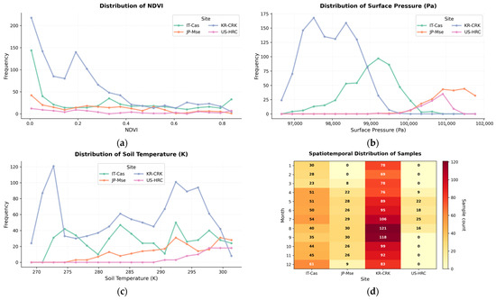
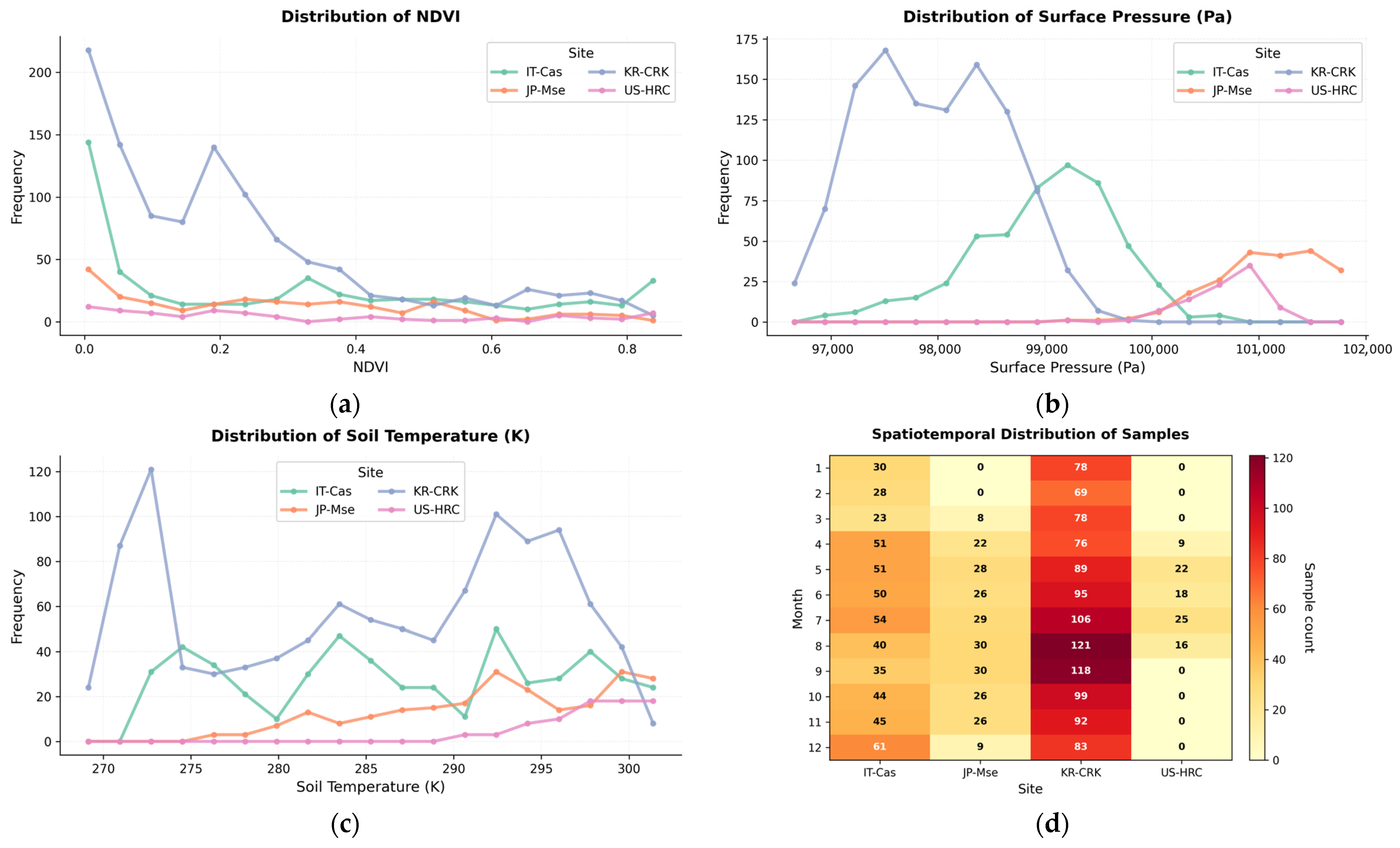
The daily model was trained using 1940 quality-controlled observations. To assess representativeness, we examined the distribution of samples across months, sites, and key environmental gradients. The dataset spans a broad range of vegetation status (NDVI), soil temperature (ST), and atmospheric conditions across the four sites, indicating coverage of diverse environmental states relevant to methane emissions (Figure 3). However, the monthly distribution is not uniform across sites (e.g., higher sample density at KR-CRK and seasonal gaps at some sites), implying that model learning may be disproportionately influenced by more frequently observed conditions. We therefore interpret the national-scale results with this sampling imbalance in mind and discuss it as a limitation.
Figure 3.
Distribution of the daily training samples across sites, seasons, and key environmental gradients. Panels show the frequency distributions of (a) NDVI, (b) SP (Pa), and (c) ST (K) for each flux site. (d) Heatmap showing the monthly distribution of samples across the four sites, illustrating seasonal and site-specific sampling density.
2.3.2. MODIS Satellite Products
Vegetation and surface water conditions were characterized using MODIS satellite data processed via the Google Earth Engine (GEE) platform (Table 2). Three MODIS-based indices—the Normalized Difference Vegetation Index (NDVI), the Normalized Difference Water Index (NDWI), and the Green Normalized Difference Water Index (GNDWI)—were derived from the daily MODIS/Terra Surface Reflectance product (MOD09GA.061) [17].
Table 2.
Summary of MODIS-derived vegetation and water indices with their respective spatial and temporal resolutions.
All indices were extracted for the 2009–2018 period and resampled to a spatial resolution of 500 m to serve as primary model inputs. Specifically, NDVI was utilized to represent vegetation vigor and phenological development, while NDWI was used to characterize vegetation water status [18]. GNDWI was incorporated to capture the flooding and drainage dynamics essential to rice paddy ecosystems [19]. Collectively, these indices provide critical spatiotemporal information on crop growth and water management, enabling the model to effectively learn the environmental drivers of methane emissions.
MODIS vegetation indices (NDVI, NDWI, and GNDWI) are provided at daily resolution and were treated as daily state variables. For the hourly model, the daily values were held constant across all hourly time steps within the same day, reflecting that vegetation structural and optical properties typically vary more slowly than meteorological drivers. Accordingly, sub-daily variability in CH4 emissions was primarily captured through hourly meteorological inputs.
2.3.3. ERA5-Land Meteorological Data
Meteorological and environmental variables were derived from ERA5-Land, a high-resolution land surface reanalysis product provided by the ECMWF. ERA5-Land provides spatially and temporally consistent data on surface atmospheric and soil conditions, encompassing key variables that influence methane dynamics.
For the 2009–2018 study period, we extracted five primary variables: soil temperature (ST), volumetric soil water (SWVL1), surface pressure (SP), total evaporation (E), and total precipitation (TP) (Table 3). These variables capture the seasonal and regional climatic variability inherent to rice paddy ecosystems. They serve as fundamental model inputs, allowing the system to learn the specific environmental conditions that govern methane production, oxidation, and transport processes.
Table 3.
Summary of meteorological and soil variables derived from the ERA5-Land dataset, including their spatial and temporal resolutions.
ERA5-Land variables available only at daily resolution were assigned uniformly to all hourly time steps within the corresponding day, rather than being temporally interpolated. This approach preserves daily water and energy constraints while allowing the model to learn sub-daily emission variability from hourly meteorological drivers.
2.3.4. HWSD Soil Data
Soil properties play a critical role in the production and oxidation of methane within rice paddy ecosystems. We utilized soil classification data from the HWSD, based on the World Reference Base for Soil Resources (WRB) classification system. The WRB is an internationally standardized framework developed by the Food and Agriculture Organization (FAO) that categorizes soils according to their formation processes, moisture regimes, and organic matter accumulation.
By applying the WRB classification, we identified the dominant soil types in rice-growing regions and incorporated the spatial distribution of soil environments conducive to anaerobic conditions—a primary driver of methane production. Furthermore, the use of this standardized system ensures consistency and extensibility across international observation sites, such as those in Italy, Japan, and USA, facilitating a robust comparative analysis.
2.3.5. Farm Map: Rice Paddy Masking Data
Rice paddy masking was performed using the Farm Map dataset, a high-resolution land-cover map provided by the National Geospatial Information Platform, operated by the Ministry of Land, Infrastructure and Transport. The Farm Map dataset provides a detailed delineation of agricultural land types throughout South Korea.
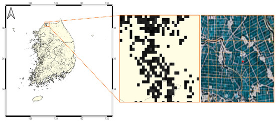
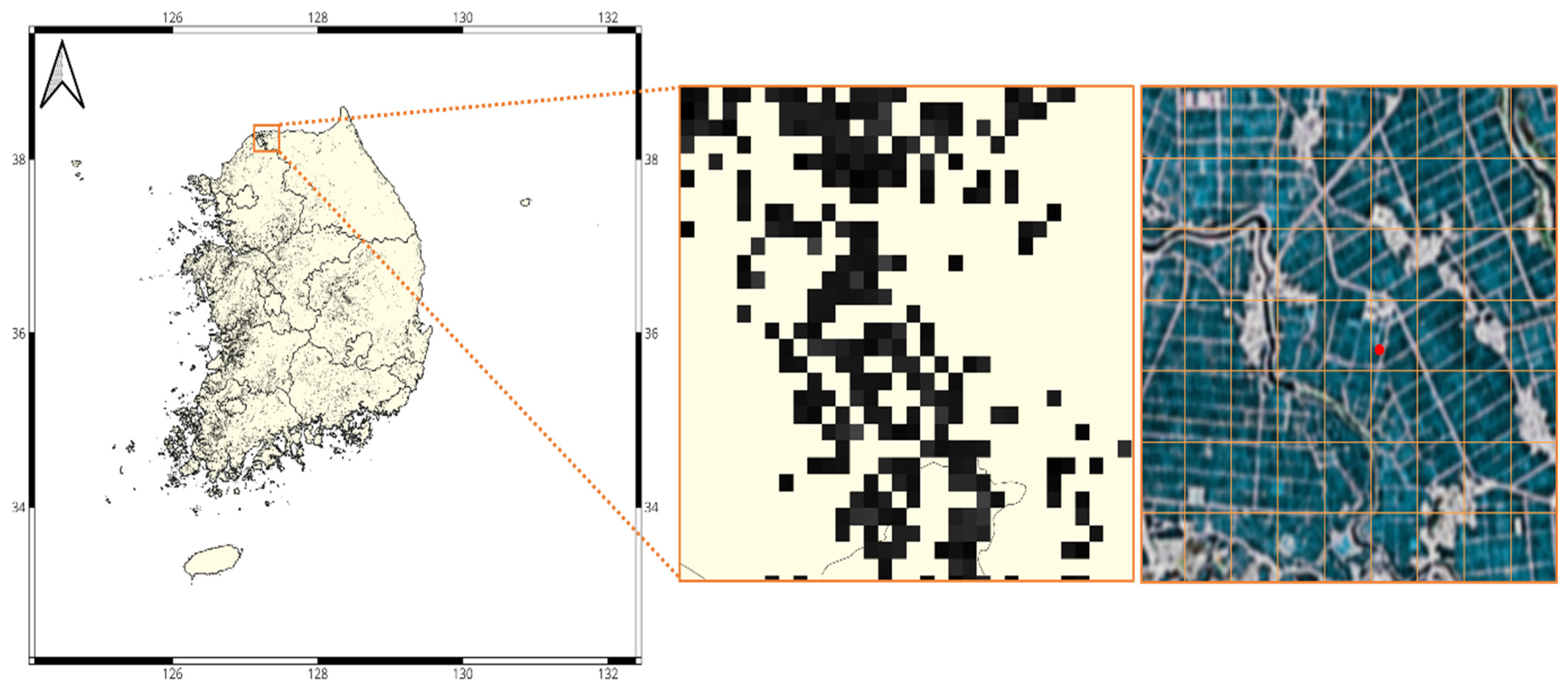
For this study, we extracted and masked only the areas classified as rice paddies. Because the analysis explicitly targets pixels classified as rice paddies, the 500 m grid cells used for model training predominantly represent homogeneous rice land cover (Figure 4). This procedure eliminates noise from non-target land-cover types and ensures that model predictions are strictly confined to regions directly associated with methane emissions from rice cultivation. All input datasets utilized in this study are publicly available and offer consistent spatiotemporal coverage. By integrating climatic, soil, vegetation, and spatial data, the resulting compiled dataset facilitates high-precision estimation of methane emissions across South Korean rice paddies.
Figure 4.
National distribution of rice paddies in South Korea and an example of their representation on a 500 m grid. The left panel shows the polygon-based rice paddy map used in this study. The middle panel illustrates the aggregation of rice paddy polygons to 500 m grid cells. The right panel provides a close-up example highlighting mixed land-use conditions within a grid cell and the assignment of an eddy covariance flux tower location.
2.4. Data Preprocessing
2.4.1. Flux Data Quality Control
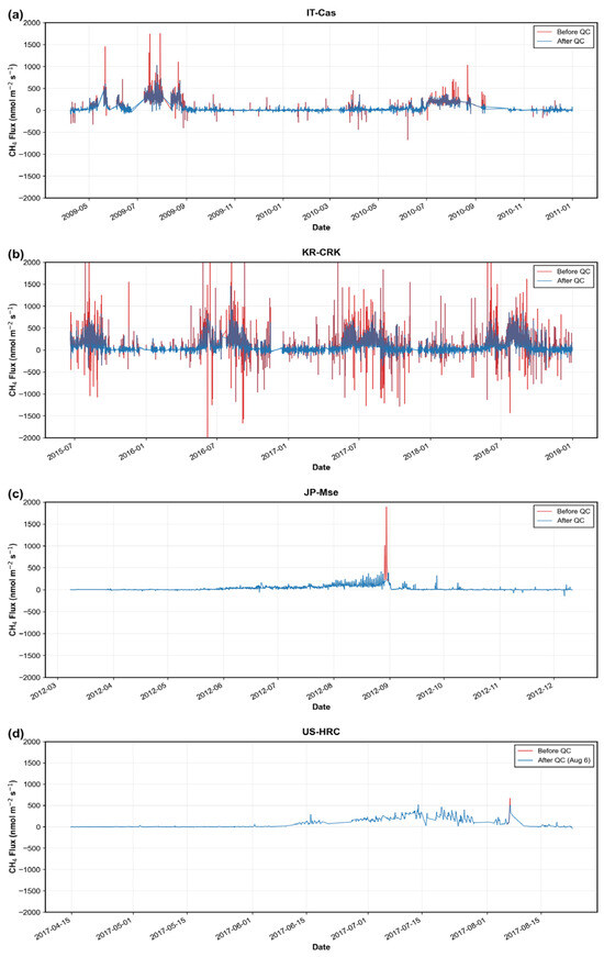
To ensure the reliability of methane flux observations, a two-stage quality control (QC) procedure was implemented. The first stage involved point-level QC to eliminate outliers and short-term spikes. Following the standardized framework of the FLUXNET-CH4 Community Product [13,14], physically implausible flux values indicative of sensor malfunction or measurement error were excluded. Specifically, CH4 flux values exceeding 1500 nmol CH4 m−2 s−1 or falling below −500 nmol CH4 m−2 s−1 were removed.
Subsequently, distribution-based criteria were applied: values outside the 1st and 99th percentiles of the overall distribution, as well as those deviating more than three times the median, were excluded. To further eliminate transient spikes caused by sensor noise or external disturbances, an additional filter was applied based on the following criteria:
- CH4 > 100 and |CH4 − Median| > 3 × Median Absolute Deviation (MAD)
As eddy covariance methane flux measurements are sensitive to turbulence conditions and instrumentation quality, their underlying assumptions and limitations were addressed in accordance with previous studies [20]. Representative examples of outliers removed during this initial QC stage are highlighted with red circles in Figure 5a,b.
Figure 5.
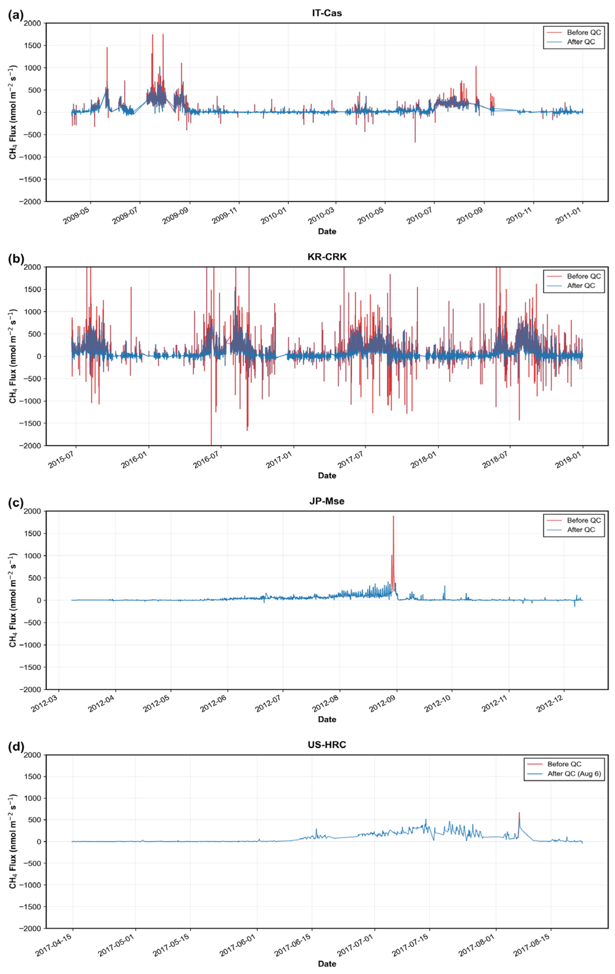
Example of quality control (QC) filtering at rice paddy flux sites: (a) IT-Cas (Castellaro, Mantua, Italy), (b) KR-CRK (Cheorwon, Gangwon, South Korea), (c) JP-Mse (Mase, Tsukuba, Japan), and (d) US-HRC (Humnoke Rice Site, AR, USA). Outlier data points (red) were removed during the first-stage QC process to eliminate extreme values and short-term spikes (a,b), and during the second-stage QC process to remove abnormal day-scale variability (c,d), leaving the cleaned dataset (blue). The x-axis range is unified from −2000 to 2000 for comparability.
In the second stage, extreme-day filtering was applied to eliminate abnormal day-scale variability persisting after point-level QC in Figure 5c,d. When extreme flux values—defined as the upper 0.5% of the distribution—were concentrated within a single day and resulted in an implausibly high daily mean, the entire day was excluded as being distorted by spikes. Furthermore, a site-cluster-specific baseline was established using the mean daily flux; days exceeding three times this baseline were identified as extremes caused by transient disturbances or operational issues and subsequently removed. This two-stage QC procedure effectively reduced measurement noise and anomalous variability, ensuring that only data with temporal continuity and physical plausibility were retained for model training and validation.
After quality control, temporal gaps remained in the hourly and daily CH4 flux time series due to data screening and instrument limitations. We did not gap-fill or interpolate these missing flux values, as doing so would introduce additional assumptions into the training data. Instead, the models were trained using only time steps with valid flux observations together with the corresponding environmental predictor variables. FLUXNET-CH4 observations were retained at their native temporal resolution. These data were used directly for the hourly model, whereas for the daily model, flux observations were aggregated from hourly to daily resolution.
2.4.2. Spatiotemporal Resolution Matching
To integrate heterogeneous datasets, a preprocessing pipeline was implemented to harmonize temporal and spatial resolutions. Ground-based CH4 flux observations from FLUXNET-CH4 were first screened for missing values and designated as the reference variable. Meteorological data from ERA5-Land and MODIS satellite products were collected for the period 2009–2018; all input datasets were subsequently resampled to a unified daily temporal resolution and a 500 m spatial resolution. MODIS-derived NDVI and NDWI were obtained from daily products via GEE, with spatial resampling applied to ensure alignment with the target resolution. Soil data from the HWSD, originally provided in binary (.bil) and Microsoft Access (.mdb) formats, were processed by extracting WRB4 soil classifications and converting them into CSV format to facilitate spatial merging based on geographic coordinates. To define the study domain, rice paddy Shapefiles from the Farm Map were rasterized to a 500 m grid. These masks were applied consistently across all variables, ensuring spatial alignment and restricting the analysis to rice cultivation areas.
Point-based CH4 flux observations from eddy covariance towers were assigned to the 500 m grid cell containing each tower location. ERA5-Land variables originally provided at 9 km resolution were resampled to 500 m using bilinear interpolation to ensure spatial consistency with MODIS-derived predictors.
2.4.3. Input Variable Suitability
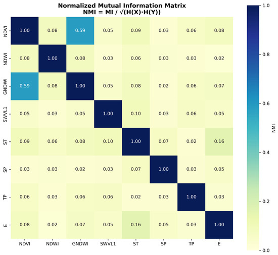
To assess redundancy among input variables, Normalized Mutual Information (NMI) was calculated for all variable pairs. The results indicated that NMI values remained below 0.1 for most combinations, suggesting limited information overlap and high independence among features (Figure 6). A relatively higher NMI was observed for the GNDWI–NDVI pair; however, this stems from the shared vegetation-related spectral characteristics inherent in both indices. Crucially, GNDWI represents the likelihood of surface water presence, whereas NDVI reflects vegetation vitality and phenology—two fundamentally different functions. Consequently, these indices capture complementary aspects of methane emission processes, providing distinct information to the model without semantic redundancy.
Figure 6.
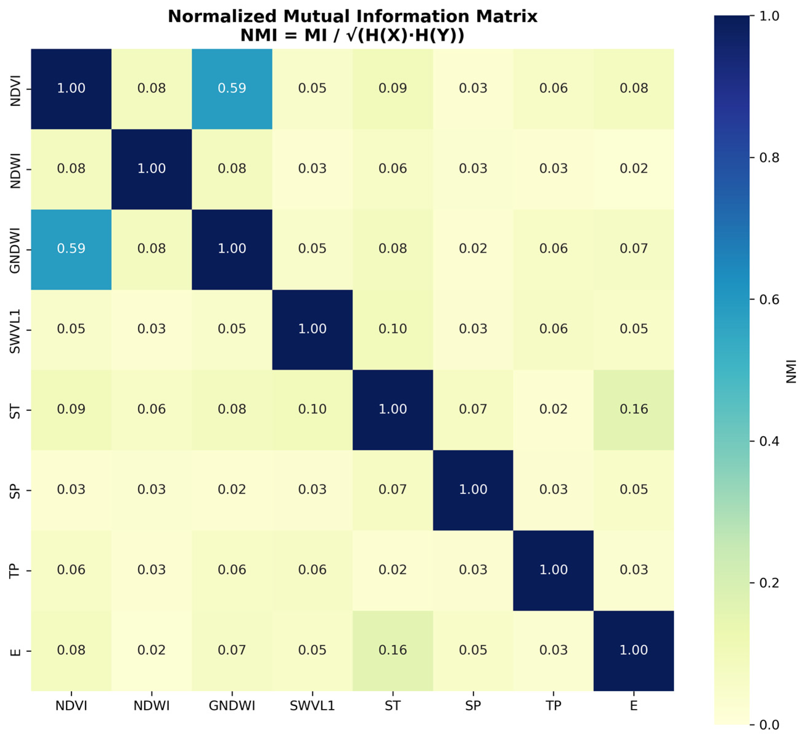
Normalized Mutual Information (NMI) matrix of the input variables. Low NMI values across most pairs indicate high statistical independence and minimal redundancy. The relatively higher NMI between NDVI and GNDWI reflects shared vegetation-related spectral characteristics; however, these indices are fundamentally distinct, representing vegetation phenology and surface water presence, respectively.
2.5. Modeling
2.5.1. Machine Learning Model
Methane prediction models were developed using Fast and Lightweight AutoML (FLAML), an efficient framework that automates algorithm selection and hyperparameter optimization through cost-aware search strategies [21]. FLAML evaluates a diverse range of regression algorithms—including gradient boosting, random forests, and ensemble methods—to identify the optimal configuration based on cross-validation performance. By minimizing the need for manual tuning, this approach allows for a comprehensive exploration of the model space, making it particularly well-suited for climate–ecosystem predictions characterized by complex, nonlinear relationships.
For large-area, high-resolution methane mapping, existing approaches such as emission factor inventories, process-based models, and remote sensing-assisted empirical methods each present practical limitations, including coarse spatial representation, extensive input and parameter requirements, or simplified empirical relationships [6,22,23].
The AutoML framework adopted in this study was therefore selected to address these constraints by enabling automated model selection and hyperparameter optimization across heterogeneous input datasets. By integrating multi-source drivers at 500 m spatial and daily temporal resolutions with minimal manual intervention, and by applying SHAP-based post hoc interpretation, the framework aims to balance predictive skill, computational efficiency, and interpretability for national-scale applications.
Separate models were trained for daily and hourly temporal resolutions, utilizing quality-controlled datasets of 1940 and 25,051 observations, respectively. The target variable for both models was CH4 flux, expressed in units of nmol CH4 m−2 s−1. Both models employed an identical set of input features:
- ERA5-Land meteorological variables: ST, SWVL1, SP, E, and TP.
- MODIS vegetation indices: NDVI, NDWI, and GNDWI.
- HWSD soil classification: WRB4.
2.5.2. Daily and Hourly Model Development
The daily model was trained using daily-averaged input variables and flux observations. This approach effectively filters out diurnal noise while emphasizing day-to-day variability, seasonal patterns, and interannual trends. This temporal resolution is particularly well-suited for capturing long-term drivers such as crop phenology, seasonal temperature progression, and water management cycles.
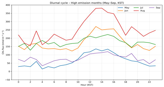
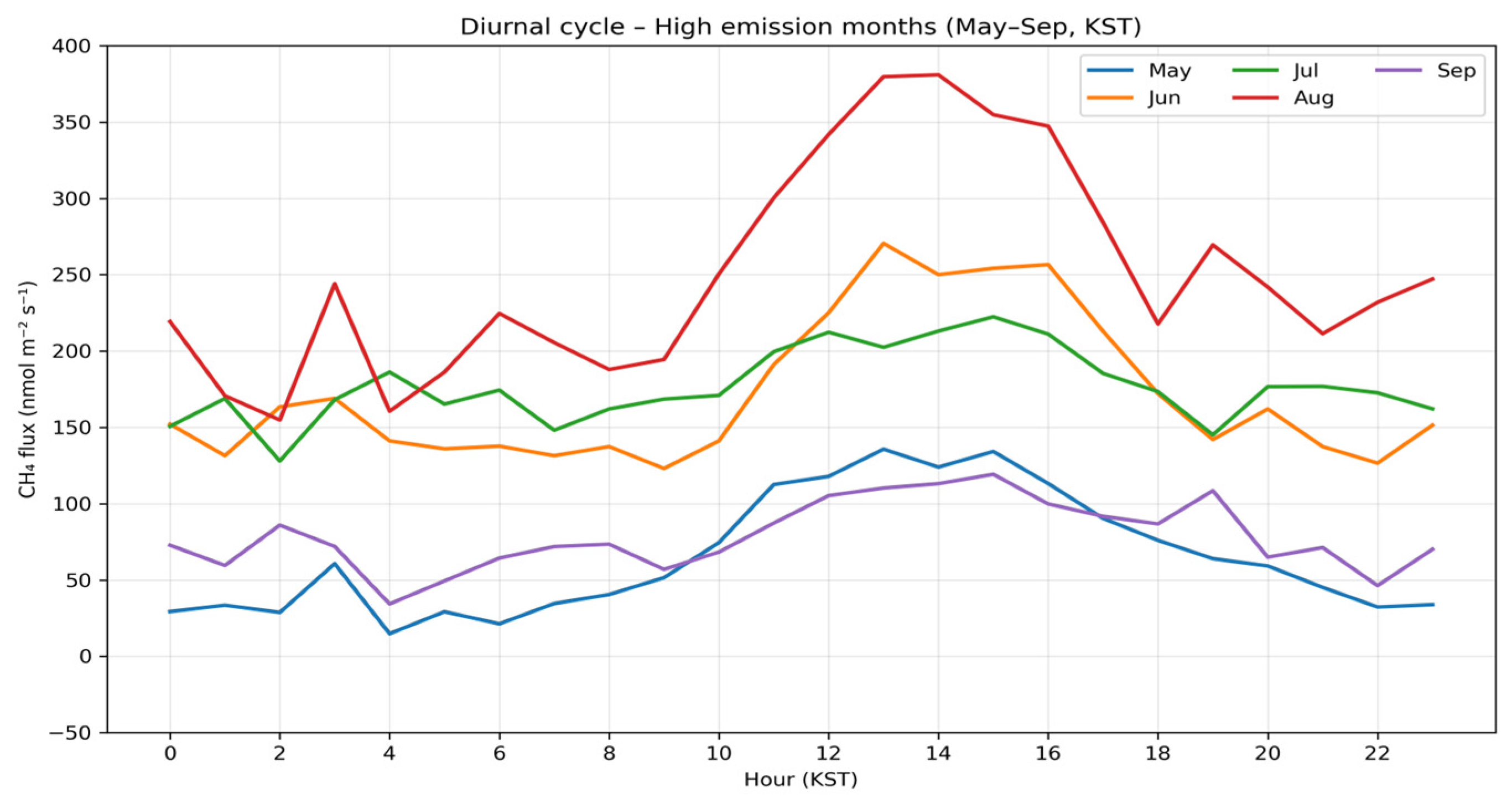
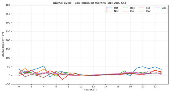
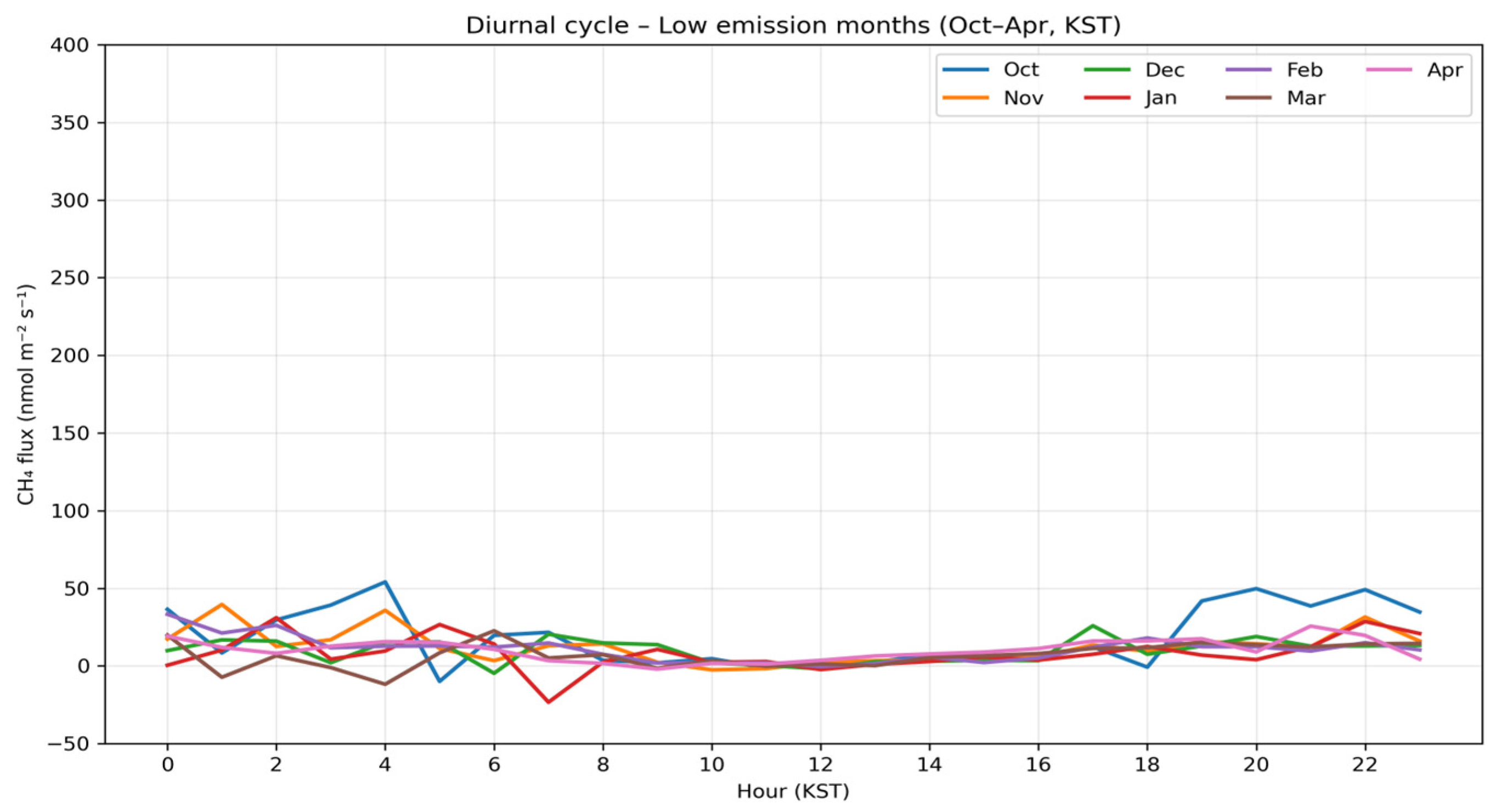
In contrast, the hourly model was designed to explicitly capture diurnal emission dynamics, including pronounced midday flux peaks during the growing season (May–September) and the variance between daytime and nighttime emissions (Figure 7 and Figure 8) [24]. Since these diurnal features are lost when data are aggregated into daily means, hourly modeling is essential for accurately reproducing sub-daily emission dynamics during high-emission periods. The parallel development of daily and hourly models—using consistent input features and validation frameworks—enables a direct comparison of how temporal resolution influences both model performance and variable importance.
Figure 7.
Diurnal variations in CH4 flux during the growing season (May–September). The curves represent monthly mean hourly averages, highlighting pronounced midday emission peaks and significant seasonal shifts in flux magnitude.
Figure 8.
Monthly diurnal variations in CH4 flux during the non-growing season (October–April). In contrast to the growing season, the flux magnitudes remain significantly lower with suppressed diurnal cycles, reflecting reduced microbial activity and altered environmental drivers during the colder months. The x-axis range is fixed for comparability.
2.6. Validation
2.6.1. Cross-Validation
To evaluate the generalization performance of the prediction models, two complementary validation strategies were employed: 5-fold and LOYO cross-validation.
In 5-fold cross-validation, the entire dataset was randomly partitioned into five subsets of equal size. Each subset served as a validation set once, while the remaining four subsets were used for training. This process was repeated five times, and the average performance across all folds was calculated to assess overall model accuracy. This approach effectively captures the data distribution and mitigates overfitting, thereby enhancing model generalization.
LOYO cross-validation partitions the data by calendar year, using one specific year for validation and the remaining years for training. This procedure is iteratively performed for each available year. LOYO explicitly tests the model’s ability to extrapolate relationships learned from specific years to independent, unseen years. Consequently, it represents a realistic validation strategy for temporally structured datasets and enables an assessment of predictive performance for future or unobserved years—a capability particularly relevant for policy-oriented applications.
For datasets with spatiotemporal structures, the integration of these two strategies is essential for evaluating both temporal and spatial generalization performance [25]. By combining AutoML-based model selection with these dual validation schemes, we minimized selection bias and established a robust prediction framework that explicitly accounts for spatiotemporal generalizability.
2.6.2. Evaluation Metrics
Model performance was quantitatively evaluated using four widely adopted regression metrics: Mean Absolute Error (MAE), Mean Bias Error (MBE), Root Mean Square Error (RMSE), and the Correlation Coefficient (CC). These metrics provide complementary perspectives on prediction error and the degree of agreement between predicted and observed values, enabling a comprehensive assessment of model accuracy, bias, and reliability.
- MBE quantifies the average signed error, indicating whether the model systematically underestimates (negative values) or overestimates (positive values) emissions. Identifying such directional bias is crucial in the context of agricultural methane emissions, as it can significantly impact mitigation planning and policy decisions; therefore, reporting MBE alongside absolute accuracy metrics is essential [26].
- MAE represents the average absolute difference between predicted and observed values, offering an intuitive measure of overall prediction accuracy. Because it treats all errors equally regardless of direction, MAE is well-suited for evaluating general performance and remains relatively insensitive to outliers, providing a stable metric across diverse methane flux ranges [27].
- RMSE is calculated as the square root of the mean squared error and, unlike MAE, assigns greater weight to larger errors. This makes it particularly effective for identifying significant prediction discrepancies and evaluating model performance under high-emission or extreme-value conditions [28].
- CC measures the strength of the linear relationship between predicted and observed values, reflecting the model’s ability to reproduce temporal or spatial patterns. CC values range from −1 to 1, with values approaching 1 indicating strong positive agreement. Even in the presence of absolute errors, CC provides valuable insight into the model’s capacity to capture relative variability and trends.
Collectively, these four metrics ensure a robust assessment of predictive performance for methane emissions from rice paddies under complex environmental conditions.
2.6.3. SHAP Analysis for Variable Importance
Shapley Additive Explanations (SHAP) analysis was employed to quantify the contribution of each input feature to the model’s predicted values [29]. SHAP values represent the marginal impact of a variable on a specific observation: a positive value indicates that the variable drives an increase in methane emissions, whereas a negative value signifies a decrease. This analysis enables the identification of dominant environmental and vegetation-related drivers and reveals how their relative importance shifts between daily and hourly temporal resolutions.
Although multicollinearity can undermine parameter stability in traditional linear regression, the tree-based models selected by the AutoML framework—such as Random Forest, Extra Trees, and Gradient Boosting—are structurally less sensitive to feature interdependence. Rather than relying on explicit coefficient estimation, these models utilize hierarchical splitting rules, making them inherently more robust to multicollinearity. Consequently, the presence of correlated input variables is expected to have a negligible impact on overall predictive performance.
2.7. Methane Mapping Procedure
2.7.1. Spatial Continuum: Extension of Point-Based Methane Prediction
Using the AutoML-based prediction models, input variables—including MODIS vegetation indices (NDVI, NDWI, and GNDWI), ERA5-Land meteorological data (SP, ST, and TP), and WRB4-based soil classifications—were applied to gridded rice paddy areas across South Korea for the period 2020–2022. This process extended the point-based methane predictions derived from flux observation sites to a high-resolution spatial continuum covering national rice cultivation areas. This step is instrumental in estimating methane emissions in regions lacking direct monitoring by leveraging the models’ spatial generalization capabilities, providing a robust foundation for analyzing the dynamic spatial distribution of emissions.
2.7.2. Generation of Daily Methane Flux Grid Maps
To ensure predictions were restricted to actual rice cultivation areas, the Farm Map dataset from the national geospatial platform was rasterized at a 500 m spatial resolution to serve as a rice paddy masking layer. On a daily basis, only grid cells classified as rice paddies within the Farm Map were extracted, ensuring that prediction results were limited to areas where methane emissions realistically occur.
Through this masking-based spatial processing, daily methane emission maps were constructed for the three-year study period (2020–2022). These maps enable intuitive visualization of spatial methane distributions and facilitate the detection of hotspots, analysis of cumulative changes across rice growth stages, and comparison of seasonal and interannual variability. Such high-resolution, raster-based spatiotemporal analyses provide essential data for developing greenhouse gas mitigation strategies in the agricultural sector and for advancing national methane monitoring systems.
3. Results
3.1. Model Performance
3.1.1. Daily Model Performance
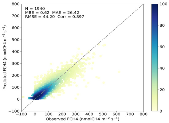
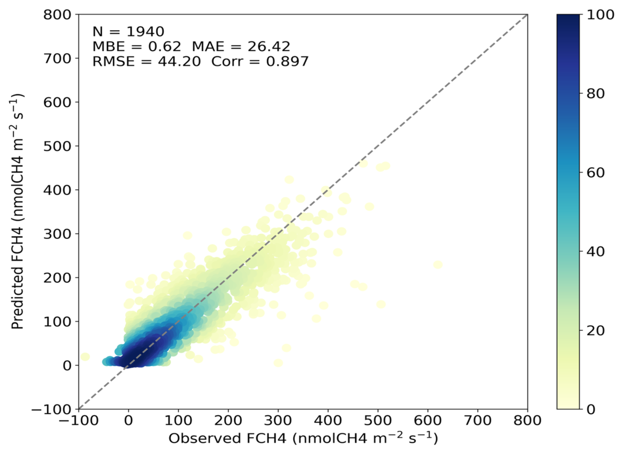
The daily model was trained on a total of 1940 observations. Based on 5-fold cross-validation, the model achieved a CC of 0.897, with an MAE of 26.42 nmol CH4 m−2 s−1 and an RMSE of 44.20 nmol CH4 m−2 s−1 (Table 4; Figure 9). The MBE was near zero, indicating the absence of systematic overestimation or underestimation across the entire observation range.
Table 4.
Performance metrics of the daily model using 5-fold cross-validation.
Figure 9.
Scatter plots of the daily model using 5-fold cross-validation.
LOYO (Leave-One-Year-Out) cross-validation was performed to evaluate temporal generalization. The model demonstrated consistently high performance, yielding an overall CC of 0.819, an MAE of 37.46 nmol CH4 m−2 s−1, and an RMSE of 58.51 nmol CH4 m−2 s−1 (Table 5). On an annual basis, CC values ranged from 0.73 to 0.91, while MAE values varied between 24 and 51 nmol CH4 m−2 s−1.
Table 5.
Performance metrics of the daily model using LOYO cross-validation.
3.1.2. Hourly Model Performance
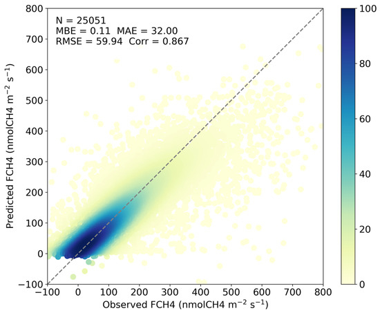
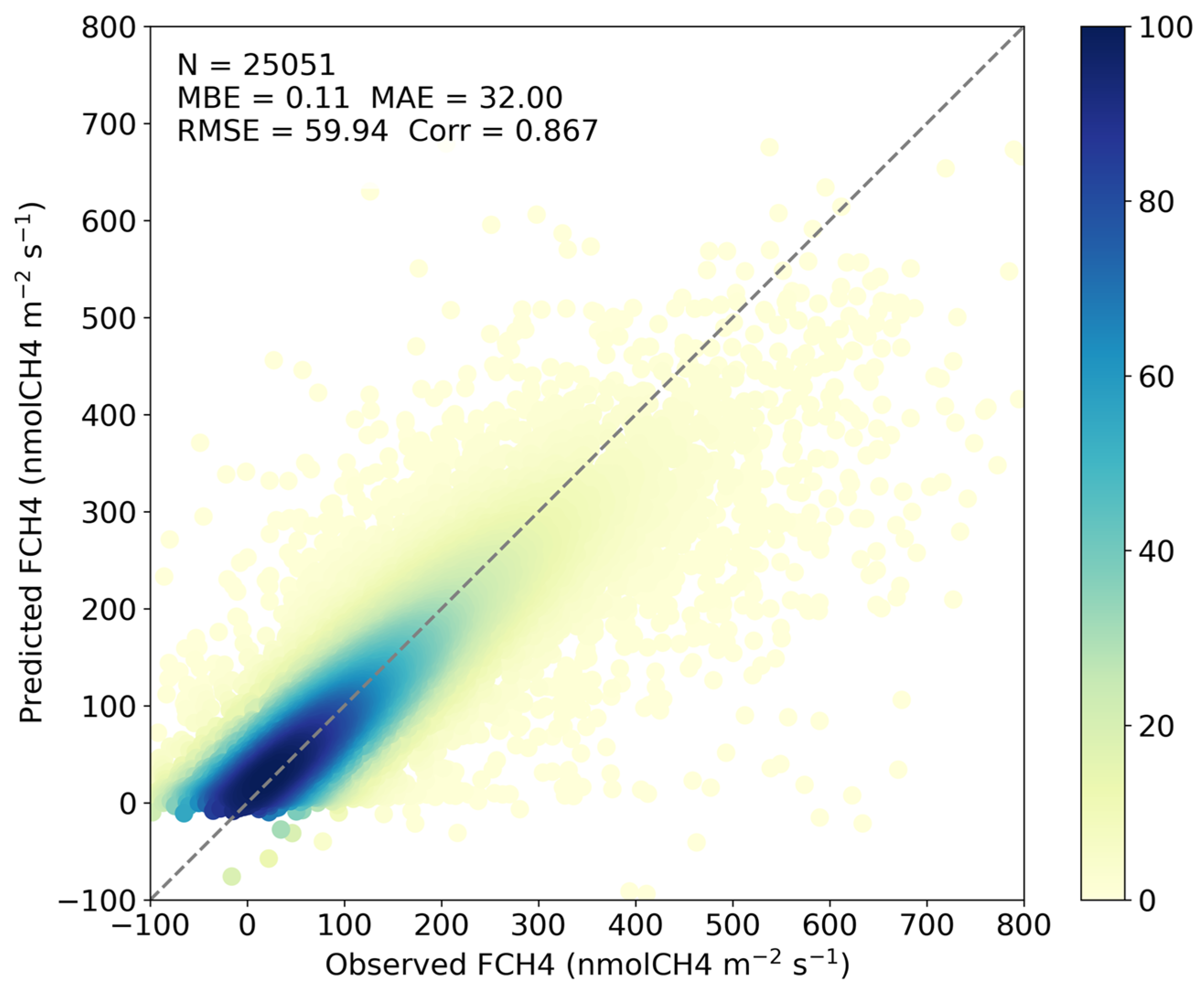
The hourly model was trained on a total of 25,051 observations. In 5-fold cross-validation, the model achieved a CC of 0.867 and an MAE of 32.000 nmol CH4 m−2 s−1 (Table 6; Figure 10). Although the CC was high, it was slightly lower than that of the daily model.
Table 6.
Performance metrics of the hourly model using 5-fold cross-validation.
Figure 10.
Scatter plots of the hourly model using 5-fold cross-validation.
In the LOYO validation, the hourly model achieved an overall CC of 0.715 and an MAE of 52.15 nmol CH4 m−2 s−1 (Table 7). Annual MAE values ranged from 33.89 to 67.34 nmol CH4 m−2 s−1, with an overall MBE of 1.06 nmol CH4 m−2 s−1. Across the LOYO folds, five out of the seven years exhibited CC values exceeding 0.7. All timestamps were standardized to KST for LOYO grouping, resulting in the exclusion of five records affected by boundary shifts. Among the four sites (IT-Cas, JP-Mse, KR-CRK, and US-HRC), no single site shows a tendency toward consistently poor performance in the hourly model (Table 7).
Table 7.
Performance metrics of the hourly model using LOYO cross-validation.
3.1.3. Model Performance Across Environmental Condition Intervals
The performance metrics of the hourly model, categorized by environmental condition intervals, are summarized in Table 8, Table 9, Table 10 and Table 11. In the soil temperature-based analysis, the normalized RMSE (nRMSE) was relatively high (4.173) at low temperatures (258.4–272.5 K) but declined sharply as temperatures rose, reaching a minimum of 0.308 in the high-temperature range (295.6–297.6 K) (Table 8). Notably, within the primary growing-season range (>287 K), the nRMSE remained consistently below 1.
Table 8.
Evaluation of hourly model performance across different soil temperature intervals.
Table 9.
Evaluation of hourly model performance across different NDVI intervals.
Table 10.
Evaluation of hourly model performance across different evaporation intervals.
Table 11.
Evaluation of hourly model performance across different seasons.
Regarding NDVI, the nRMSE was approximately 1.2 in low vegetation intervals but improved significantly to 0.3–0.5 as NDVI increased (Table 9). A similar trend was observed in the evaporation-based analysis; the nRMSE rose to approximately 1.3 under near-zero evaporation, although MAE values in this range remained low (14–20 nmol CH4 m−2 s−1) (Table 10). As evaporation increased, the nRMSE decreased to 0.2–0.6, with bias remaining within ±1 across all intervals. Seasonal analysis revealed that during the peak growing season (June–August), the MAE and nRMSE ranged from 22–25 nmol CH4 m−2 s−1 and 0.48–0.53, respectively. During transitional periods (April–May and September–October), the MAE was stable at approximately 24 nmol CH4 m−2 s−1 (Table 11), while winter months exhibited relatively higher nRMSE values. The high nRMSE in the low-temperature range is primarily attributed to the small magnitude of the mean CH4 flux during winter, rather than a lack of model precision.
3.2. Variable Importance
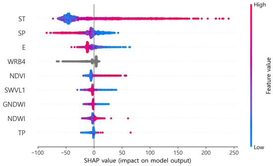
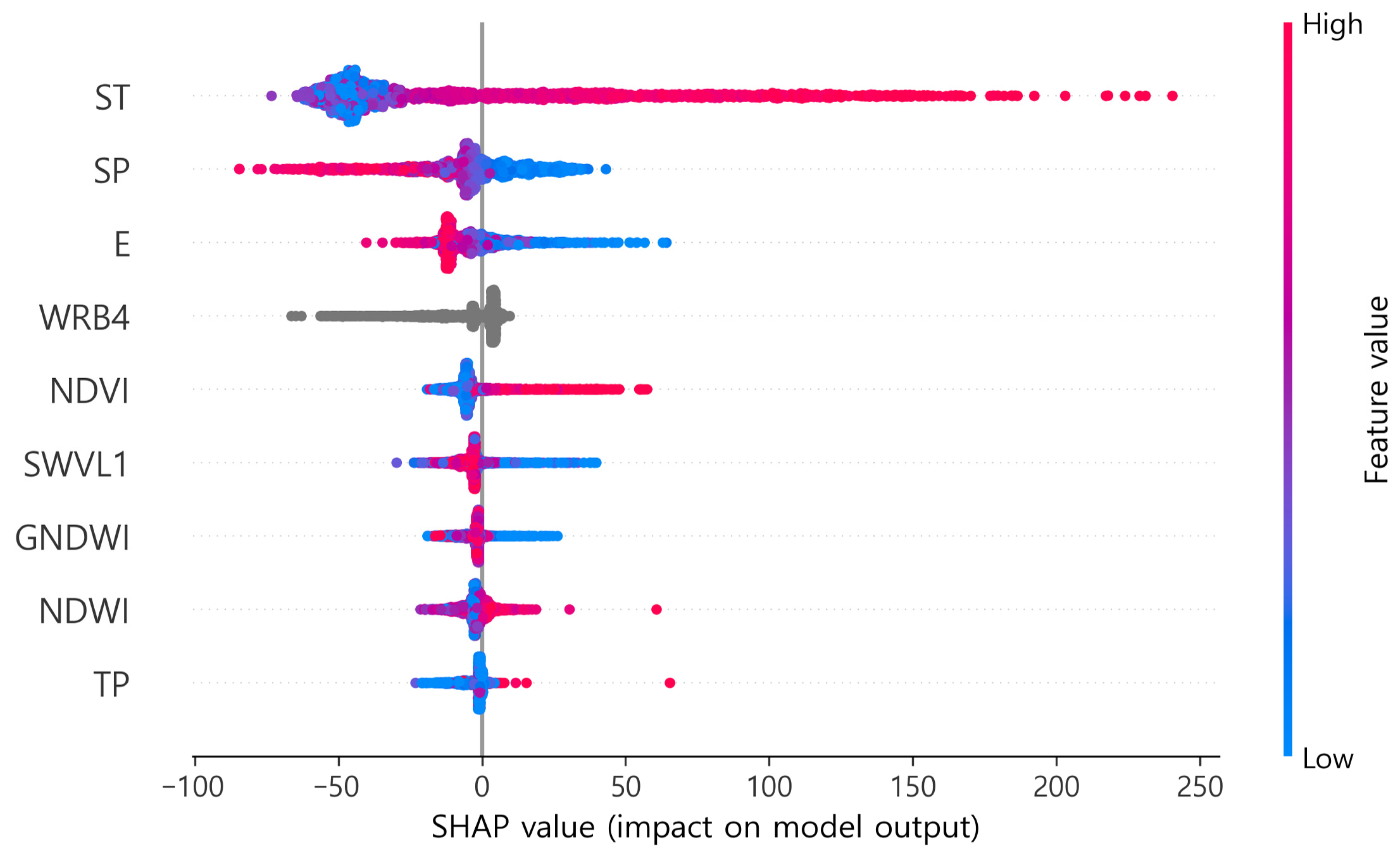
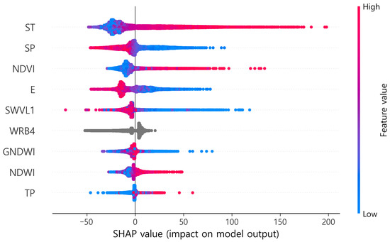
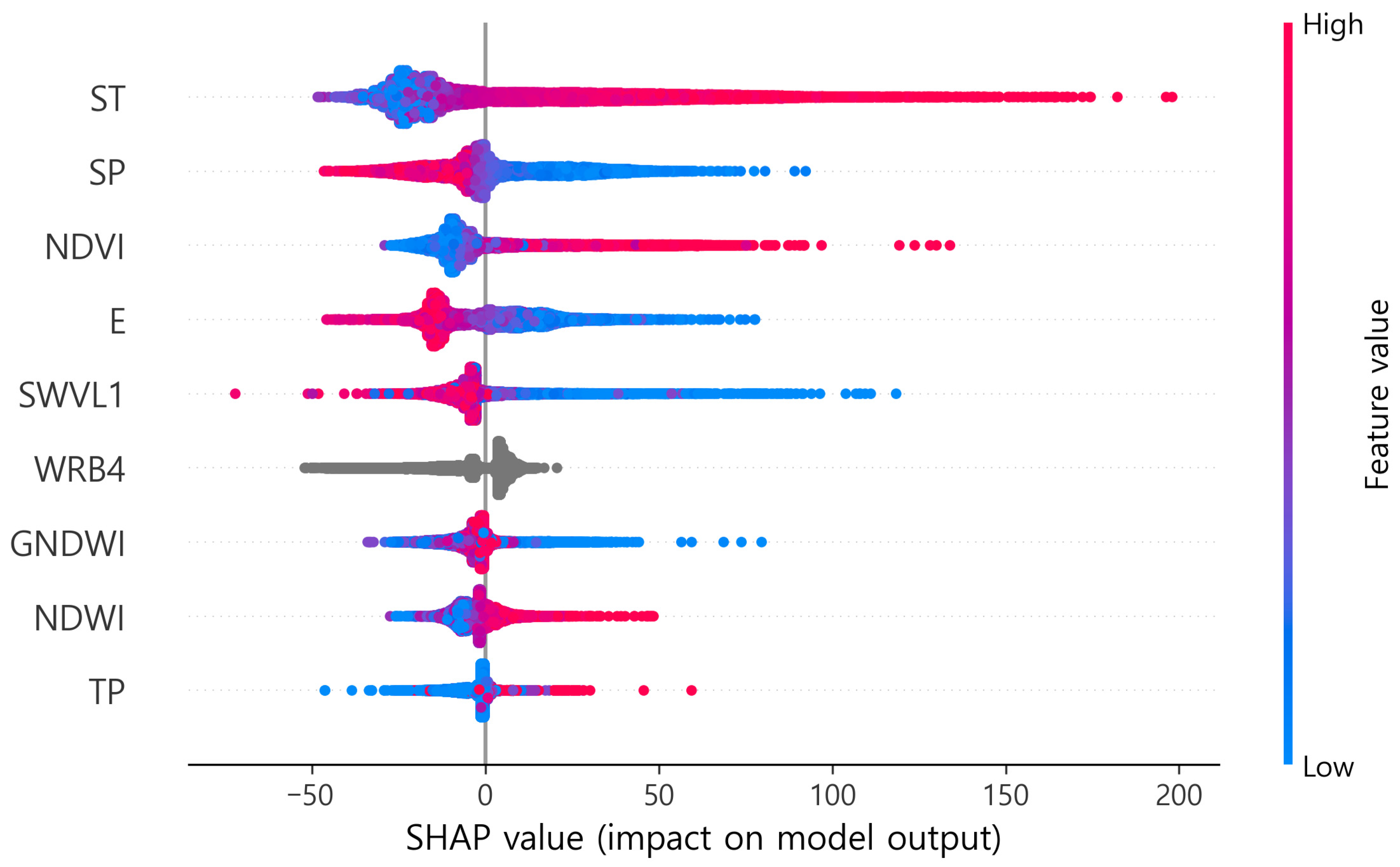
SHAP analysis revealed distinct variable importance structures between the daily and hourly models (Table 12 and Table 13; Figure 11 and Figure 12). In the daily model, ST emerged as the most dominant driver with a SHAP value of 50.19, accounting for approximately half of the total contribution. This was followed by SP (13.97), E (9.16), and WRB4 (7.94). Conversely, NDVI (7.59) and SWVL1 (5.33) exhibited relatively lower importance. In the hourly model, however, the importance was more distributed across multiple variables, including ST (27.88), SP (13.20), NDVI (12.81), E (12.47), and SWVL1 (8.24). Notably, the relative contribution of ST decreased from approximately 50% in the daily model to about 28% in the hourly model, while the importance of NDVI and SWVL1 increased by approximately 1.7 and 1.5 times, respectively.
Table 12.
Contribution of predictor variables to the daily model performance, ranked by SHAP magnitude.
Table 13.
Contribution of predictor variables to the hourly model performance, ranked by SHAP magnitude.
Figure 11.
SHAP summary plot illustrating the feature importance and their impact on the daily model’s output.
Figure 12.
SHAP summary plot illustrating the feature importance and their impact on the hourly model’s output.
3.3. Model Evaluation and Spatial Application for Korean Rice Paddies
3.3.1. Temporal Evaluation of the Daily Model at the Korean Site
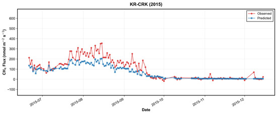
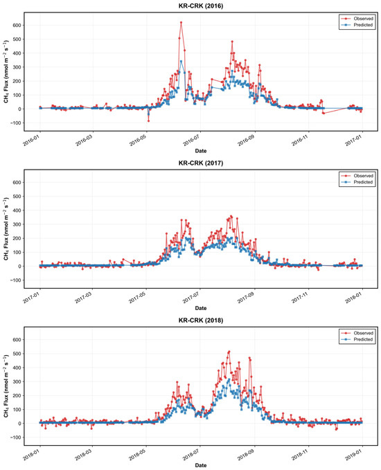
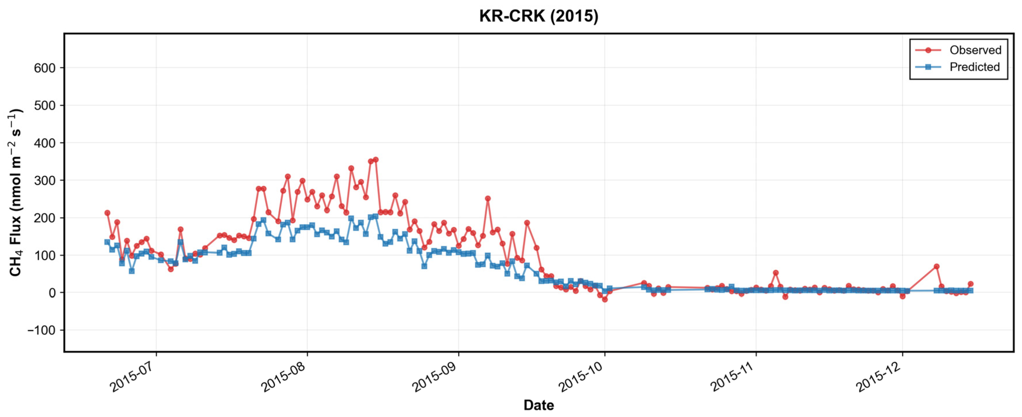
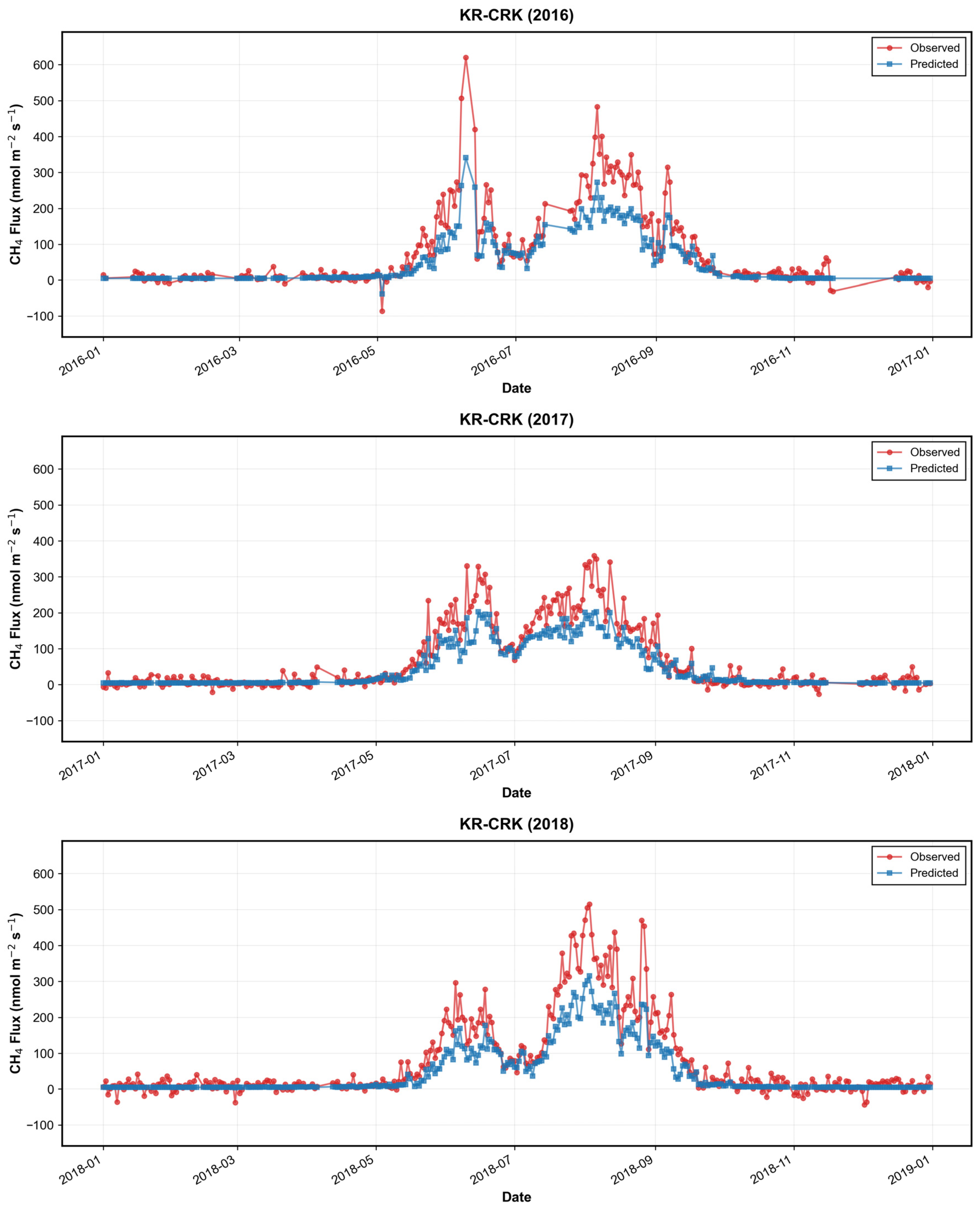
Figure 13 compares observed CH4 fluxes with daily model predictions at the Korean rice paddy site (KR-CRK) for the 2015–2018 period. The model successfully captured seasonal variations corresponding to transplanting, growing, and harvesting periods across all years. Furthermore, it adequately reproduced both the peak emissions during the summer growing season and the minimal emissions during fallow periods. Notably, during the mid-growing season (late June to July)—a period characterized by a temporary decrease or a slowdown in the increasing trend of observed emissions—the model predictions consistently aligned with the overall observed trends.
Figure 13.
Year-by-year comparison between observed and predicted daily CH4 fluxes at the KR-CRK site from 2015 to 2018. The red lines with circles represent the observations from eddy covariance, while the blue lines with squares denote the daily model predictions. The plots illustrate the model’s ability to capture seasonal dynamics, including the high emission peaks during the summer growing season and the near-zero fluxes during fallow periods.
3.3.2. Spatial Mapping of Monthly Methane Emissions Across Korean Rice Paddies
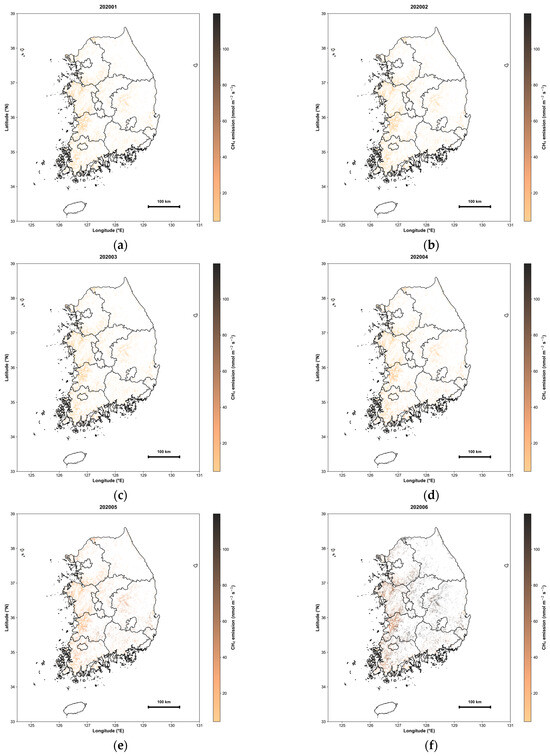
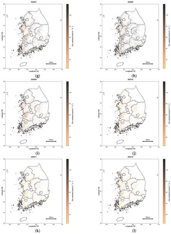
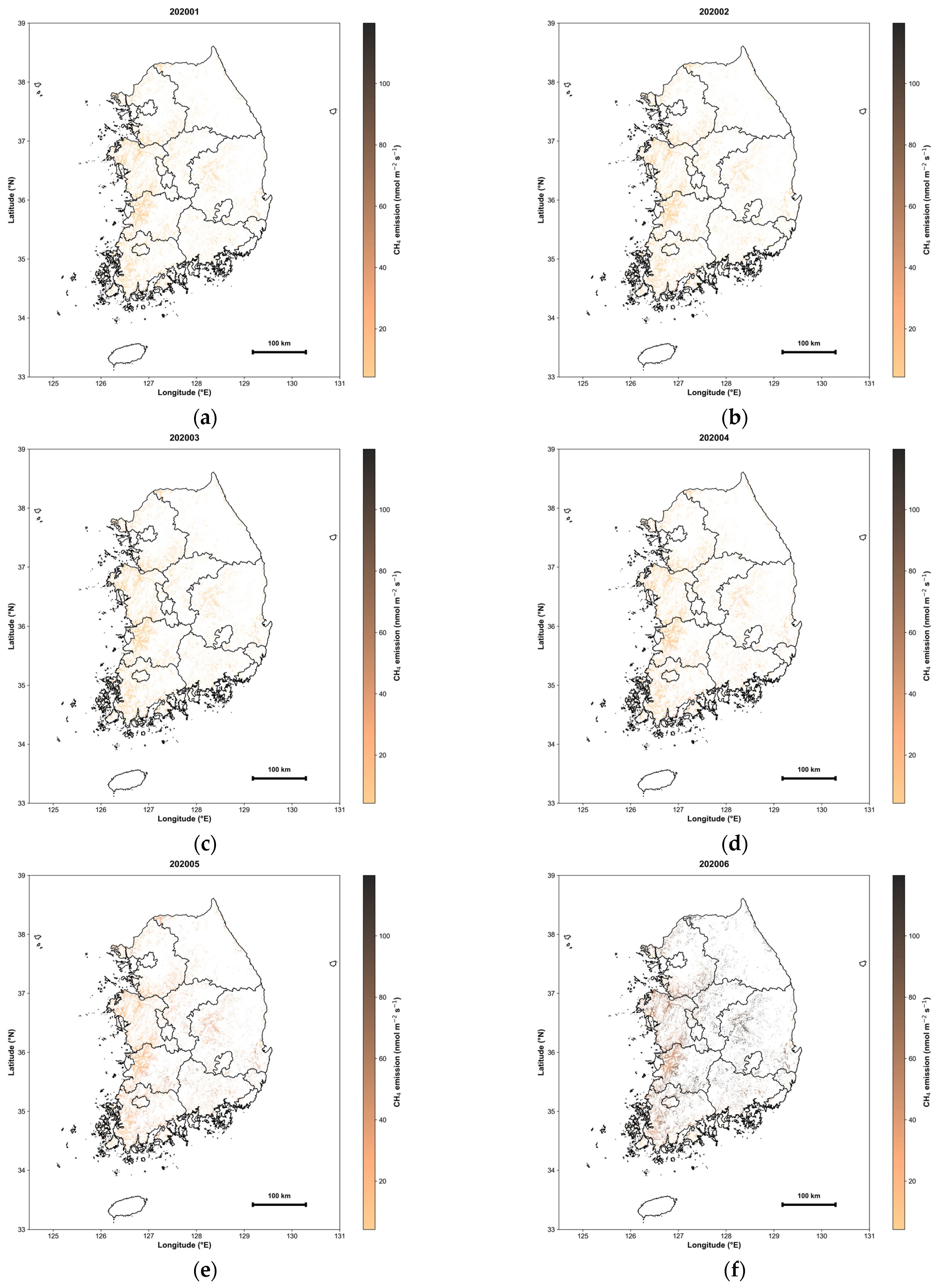
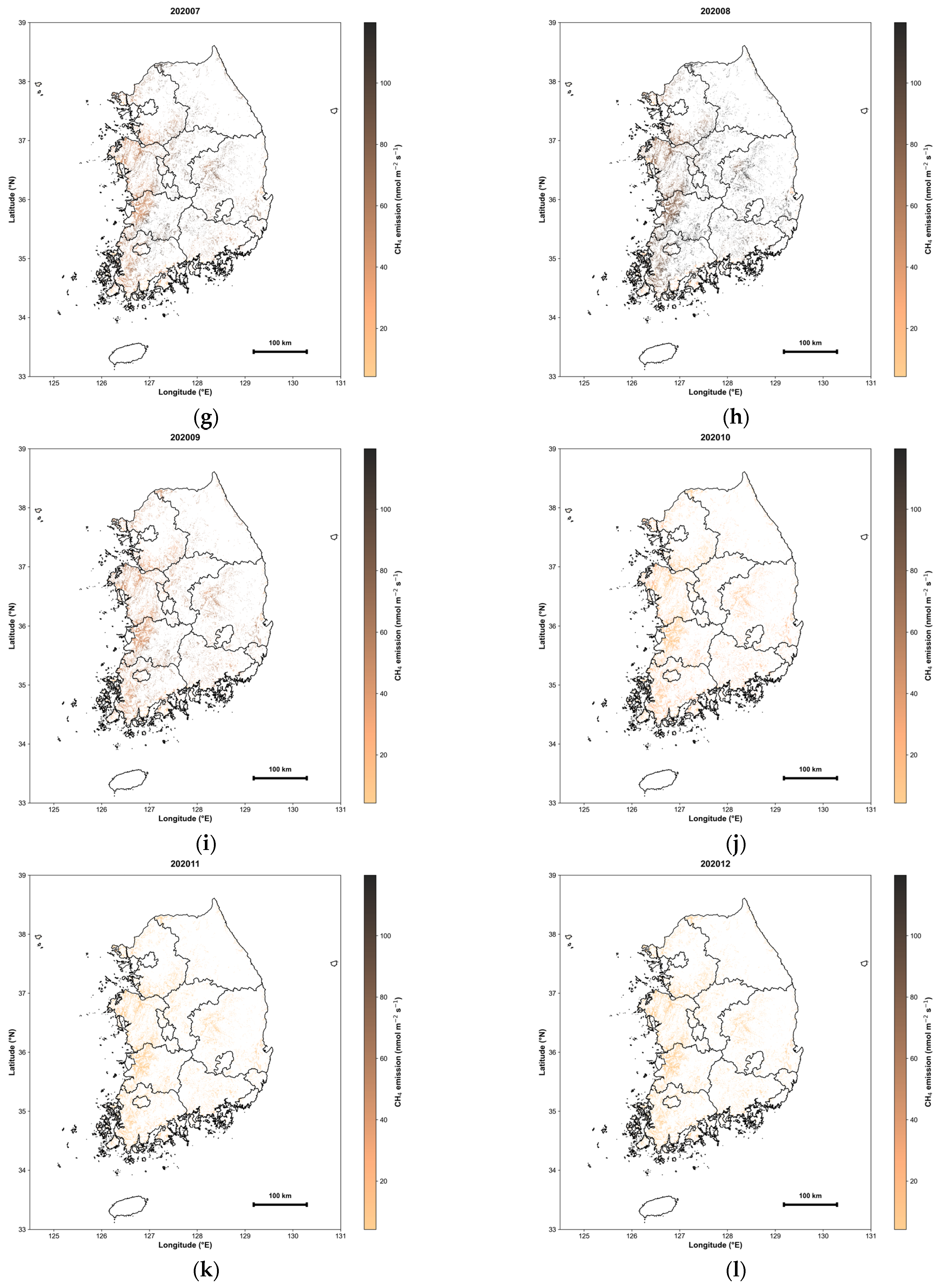
The daily model was applied to a 500 m grid across South Korean rice paddy areas for the 2020–2022 period. Daily emission maps were generated and subsequently aggregated into monthly means to analyze spatiotemporal patterns (Figure 14). CH4 emissions exhibited a distinct seasonal periodicity, reflecting stage-specific agricultural practices alongside hydrological and climatic conditions. Spatially, the recurrent formation of high-emission clusters was observed during specific periods.
Figure 14.
Monthly mean gridded CH4 emission maps for South Korean rice paddies in 2020 (nmol CH4 m−2 s−1: (a–l) represent January through December, respectively. The maps illustrate the spatiotemporal evolution of emissions, highlighting the transition from low-emission fallow periods to high-emission peaks during the peak growing season.
From January to April, most paddies remained drained, with mean emissions staying below 50 nmol CH4 m−2 s−1. Following the onset of transplanting-related flooding in May, emissions increased markedly across flooded regions. During the peak growing season (July–August), extensive high-emission areas—with monthly means exceeding 200 nmol CH4 m−2 s−1—emerged in major rice-producing provinces, including Jeollanam-do, Jeollabuk-do, Chungcheongnam-do, and Gyeonggi-do. Some of these regions exhibited even higher emission hotspots. In September and October, emissions dropped rapidly to approximately 100 nmol CH4 m−2 s−1 as fields were drained for harvest, further declining to below 50 nmol CH4 m−2 s−1 by year-end.
3.3.3. Uncertainty Mapping of Daily Methane Emission Estimates
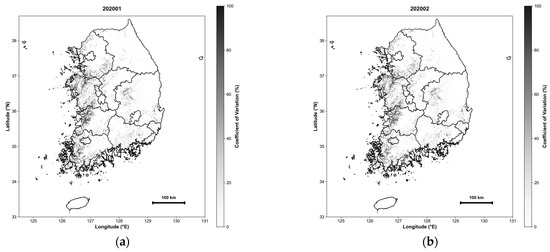
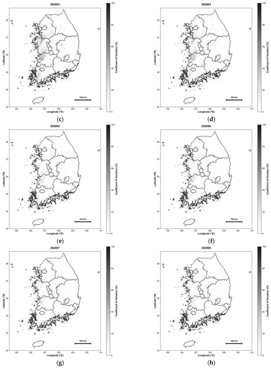
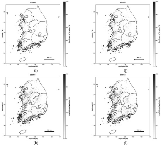
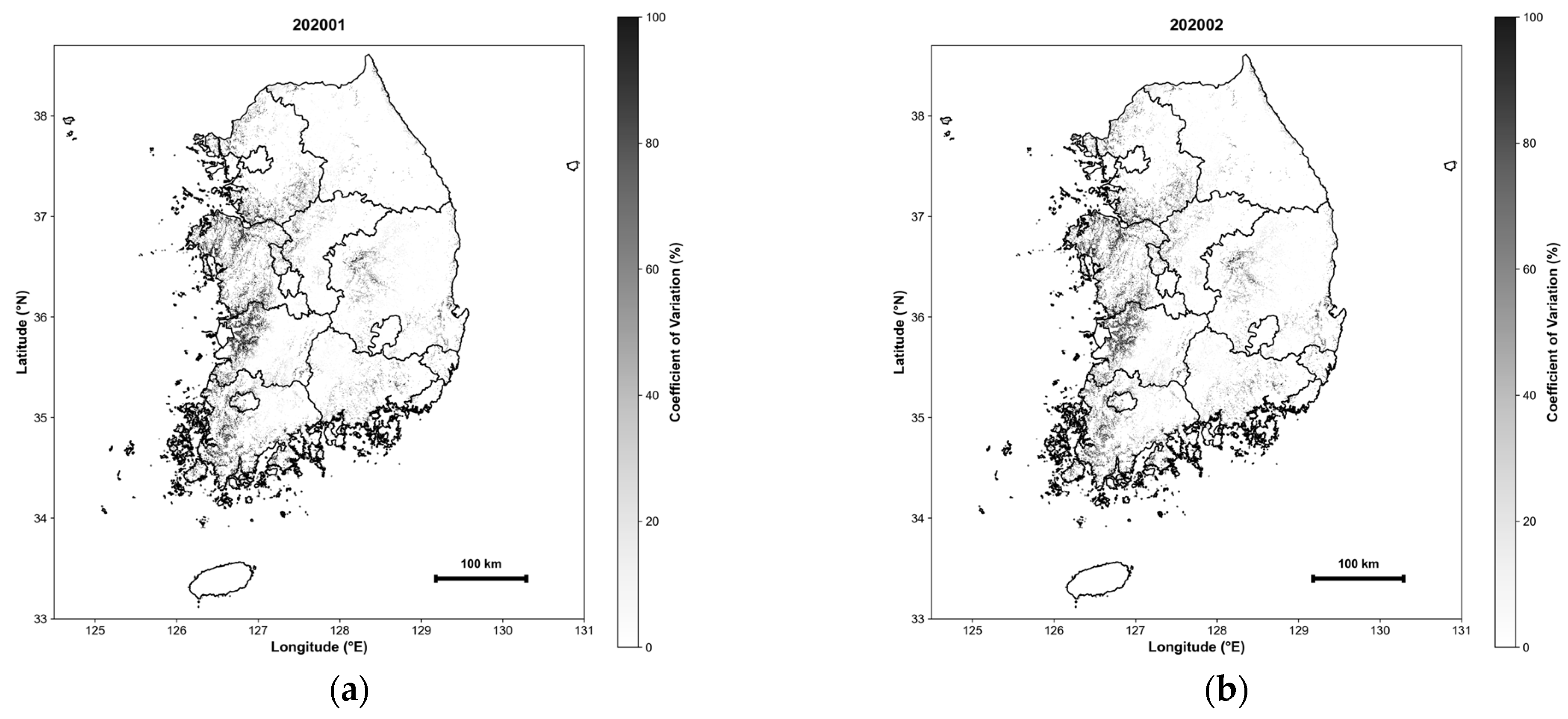
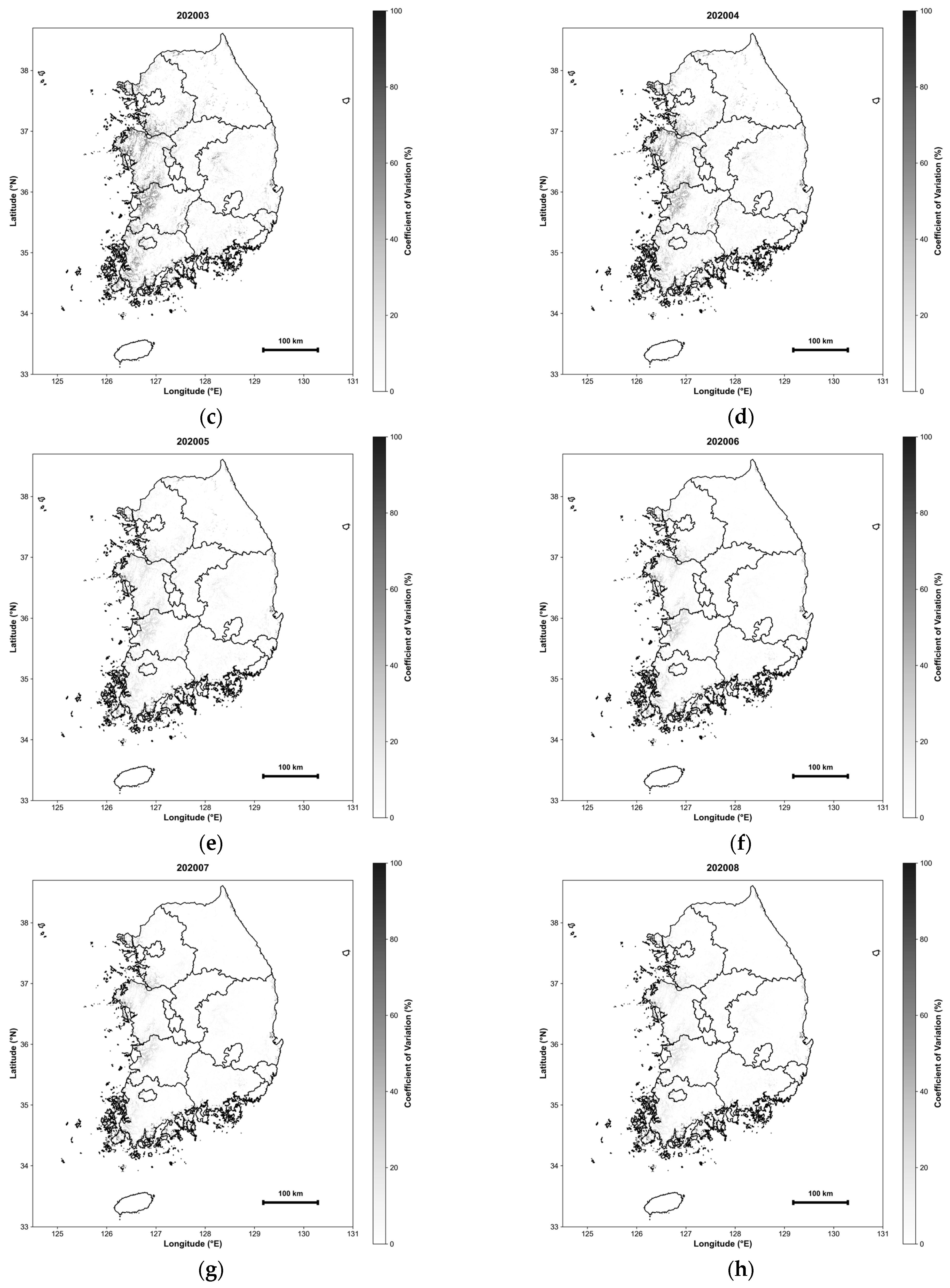
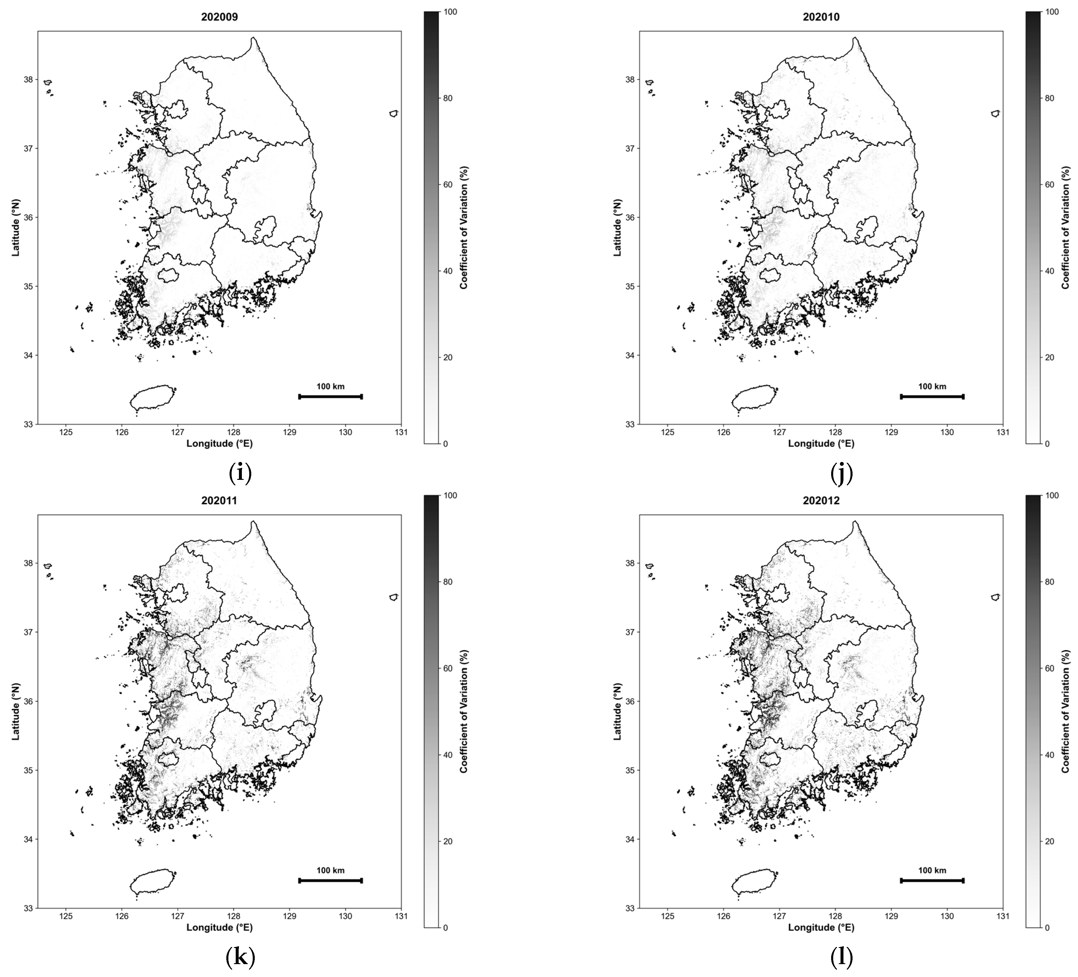
To spatially characterize the predictive uncertainty within the emission maps, we quantified the dispersion of model outputs using the coefficient of variation (CV = [standard deviation/mean] × 100) of the monthly mean CH4 emissions. For each grid cell and month, the CV was calculated across predictions generated by 21 distinct machine-learning model configurations including random forest (RF), extremely randomized trees (ERT), gradient boosting regression (GBR), and adaptive boosting (AdaBoost). This approach captures inter-model dispersion as a proxy for model-dependent uncertainty, reflecting the sensitivity of the mapped emissions to alternative algorithms and training variants rather than the temporal variability of CH4 fluxes.
The resulting uncertainty maps exhibit a pronounced seasonal pattern (Figure 15). Higher relative uncertainty is observed during the non-growing season (November–February), while lower uncertainty prevails during the main growing period (May–August). The elevated wintertime CV is primarily attributable to a low-mean effect, where CH4 emissions approach zero and small absolute prediction discrepancies result in disproportionately large relative CV values. In contrast, predictions across model configurations are more consistent during the growing season, yielding lower relative uncertainty and supporting more robust spatial interpretations during peak-emission periods.
Figure 15.
Monthly uncertainty maps of daily methane emission estimates over South Korean rice paddies, quantified by the coefficient of variation (CV). Panels (a–l) represent January through December, respectively. The CV was calculated for each pixel-month based on predictions from 21 alternative machine learning models including random forest (RF), extremely randomized trees (ERT), gradient boosting regression (GBR), and adaptive boosting (AdaBoost).
4. Discussion
4.1. Trade-Offs Between Daily and Hourly Models: Accuracy, Efficiency, and Applicability
A comprehensive comparison of the validation results reveals that the daily and hourly models offer complementary strengths, each suited to distinct applications. Consistent with the validation results (Table 4, Table 5, Table 6 and Table 7), the daily model outperformed the hourly model, showing higher correlation coefficients and lower error metrics. This superiority is likely due to the daily averaging process, which attenuates measurement noise and high-frequency variability, thereby facilitating more stable predictions. In particular, the enhanced temporal generalization of the daily model in LOYO validation suggests that seasonally recurring processes and water management schedules are more consistently captured at a daily scale.
In contrast, despite the inherent challenges of training on methane flux data with high short-term variability, the hourly model achieved stable performance across multiple years and international sites. This demonstrates the model’s robustness and its ability to effectively reproduce both seasonal and diurnal emission patterns in unobserved years. However, the differences in computational efficiency are pronounced; the hourly model requires 24 times more input data than the daily model, imposing significantly higher storage and post-processing burdens. For large-scale applications, such as national methane mapping using 500 m grids, these costs must be carefully weighed.
Empirically, daily resolution proved to be a pragmatic choice that balances predictive performance with practical applicability. Nevertheless, the hourly model holds distinct scientific value by capturing information lost through daily averaging. High-resolution analysis is essential for identifying episodic events like ebullition, which can contribute substantially to total emissions but occur over very short durations. Consequently, while the daily model is ideal for national inventory development and long-term policy evaluation, the hourly model is better suited for investigating emission mechanisms and designing real-time monitoring systems. This study underscores the importance of selecting a temporal resolution aligned with specific research objectives.
4.2. Process Interpretation from Variable Importance Across Temporal Resolutions
The variable importance analysis demonstrates that temporal resolution fundamentally alters the environmental processes that emerge as dominant controls. In the daily model, ST accounted for approximately half of the total contribution, appearing as the primary driver. This suggests that under daily averaging, gradual thermal regulation—associated with seasonal temperature fluctuations—governs methane emission variability. In contrast, the importance of variables like NDVI and SWVL1 was relatively diminished, likely because their short-term variations are smoothed during the averaging process.
Conversely, the hourly model revealed a more complex, multivariate dependency structure, where ST, NDVI, SWVL1, SP, and E all exhibited significant importance. At this finer temporal resolution, the model evaluates the specific environmental conditions required for an emission event to occur—for instance, determining the necessary level of vegetation (NDVI) for a given temperature and pressure at that specific hour. The statistical contribution (SHAP value) of NDVI is captured more prominently in the hourly model than in the daily model. As the temporal resolution increases, the broad thermal control effect becomes relatively diluted; instead, variables that represent localized and transient characteristics, such as NDVI and SWVL1, carry greater weight in explaining the short-term emission dynamics. This suggests that these factors act as more direct drivers of hourly methane variability, reflecting the intricate biogeochemical interactions that occur within shorter timeframes.
Furthermore, the elevated importance of surface pressure and evaporation indicates that physical and biogeochemical processes—such as turbulent mixing intensity, ebullition triggering, and immediate post-precipitation responses—play a pivotal role in hourly emission dynamics. These findings imply that the choice of temporal resolution is a critical factor that shapes the interpretative direction of methane emission mechanisms, even when utilizing identical input datasets. Consequently, our results suggest that while daily models are robust for carbon accounting, hourly models are indispensable for a high-fidelity understanding of the biogeochemical pathways of methane emissions.
4.3. Comparison with Existing Rice Paddy Methane Estimation Approaches
Previous rice paddy methane (CH4) estimation approaches include emission factor (EF)-based inventories, process-based models (e.g., DNDC), and remote sensing-assisted empirical or data-driven methods. EF inventories are suitable for national reporting but offer limited spatial detail, whereas process-based models are mechanistically interpretable yet require extensive inputs and parameterization. RS-based approaches enable spatial upscaling but are often constrained by relatively coarse spatial and/or temporal resolution [6,22].
In this context, our AutoML framework integrates multi-source environmental drivers to generate 500 m daily CH4 emission estimates with minimal manual tuning, while SHAP-based post hoc interpretation facilitates comparison of dominant controls with previous mechanistic and RS-based studies. Representative approaches and reported drivers are summarized in Table 14 to contextualize the proposed framework without re-implementing existing models.
Table 14.
Comparison of representative approaches for rice paddy CH4 estimation. Dominant drivers are summarized as reported in the original studies.
Temperature has been widely reported as a primary control on daily CH4 emissions, consistent with its dominance in our daily model. By contrast, the increased contribution of vegetation (NDVI) and moisture-related proxies in the hourly model suggests a timescale-dependent shift in dominant controls that may be obscured under coarser temporal aggregation.
4.4. Performance Under Different Environmental Regimes
Analysis across environmental condition intervals indicates that the hourly model performs particularly well during high-emission periods, which contribute most significantly to annual totals. This is a critical finding, given that methane emissions from rice paddies are highly concentrated within specific seasonal windows. In the soil temperature-based analysis, relative errors decreased sharply as temperatures rose, with the nRMSE remaining below 1.0 across all intervals within the primary growing-season range. Conversely, while relatively larger errors occurred at lower temperatures, their impact on annual emission estimates is considered limited due to the negligible absolute flux levels during these periods.
Furthermore, the NDVI-based analysis showed that model performance peaked under conditions of well-developed vegetation. This aligns with the established role of plant-mediated transport as a primary pathway for methane release during the growing season [30], suggesting that predictive stability improves when methane flux signals are more pronounced. Seasonal analysis corroborated these findings, demonstrating robust performance during the growing and transitional seasons, despite higher uncertainty in winter. Ultimately, these results confirm that the hourly model is highly reliable under the key conditions that govern annual methane budgets, ensuring that uncertainties during low-emission periods do not pose a substantial practical limitation.
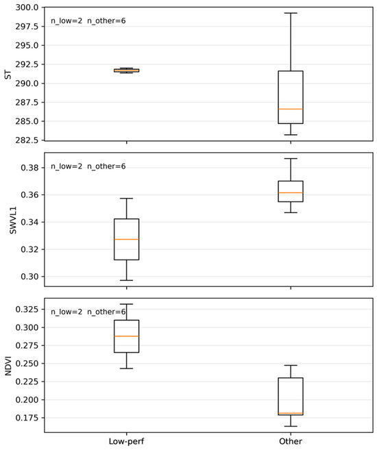
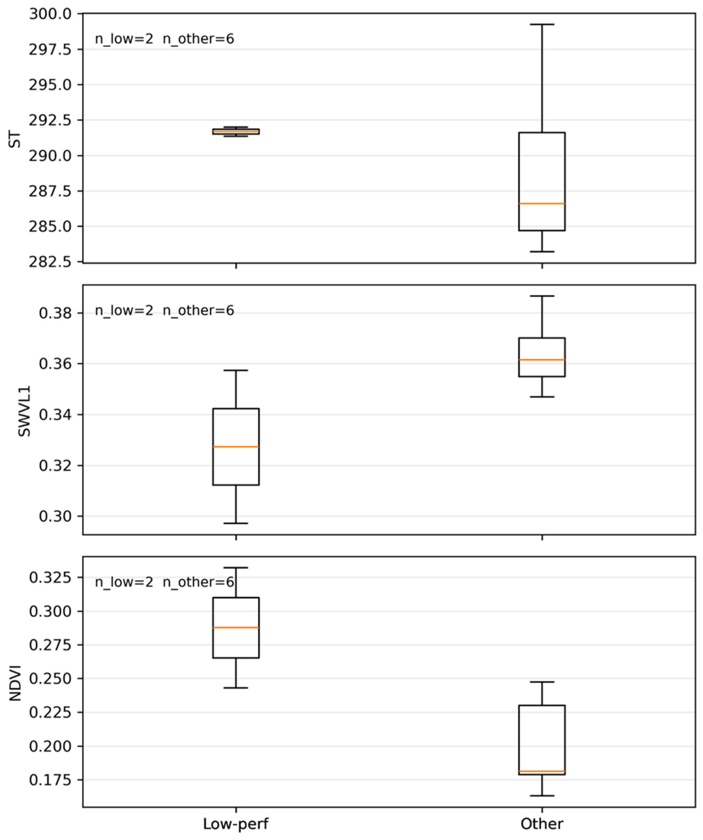
To explore the causes of performance degradation under LOYO validation, we examined two representative low-performance cases in the daily model (2009 at IT-Cas and 2015 at KR-CRK). Using daily matchup data, we compared key environmental variables between these low-performance years and other years (Figure 16). The low-performance years exhibit distinct distributions of ST, SWVL1, and vegetation indices that frequently fall outside the interquartile range of other samples. This indicates that reduced LOYO performance is mainly associated with limited temporal generalization to anomalous interannual environmental conditions rather than simple overfitting. This reflects the limited representation of anomalous interannual conditions in the training data and is discussed further in Section 4.7.
Figure 16.
Site-year median distributions of key environmental variables for representative low-performance years (2009 at IT-Cas and 2015 at KR-CRK), compared with other years.
4.5. Seasonal Coupling Between Soil Temperature and CH4 Fluxes
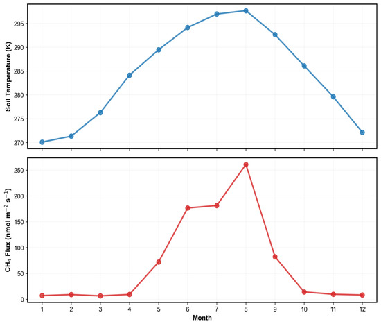
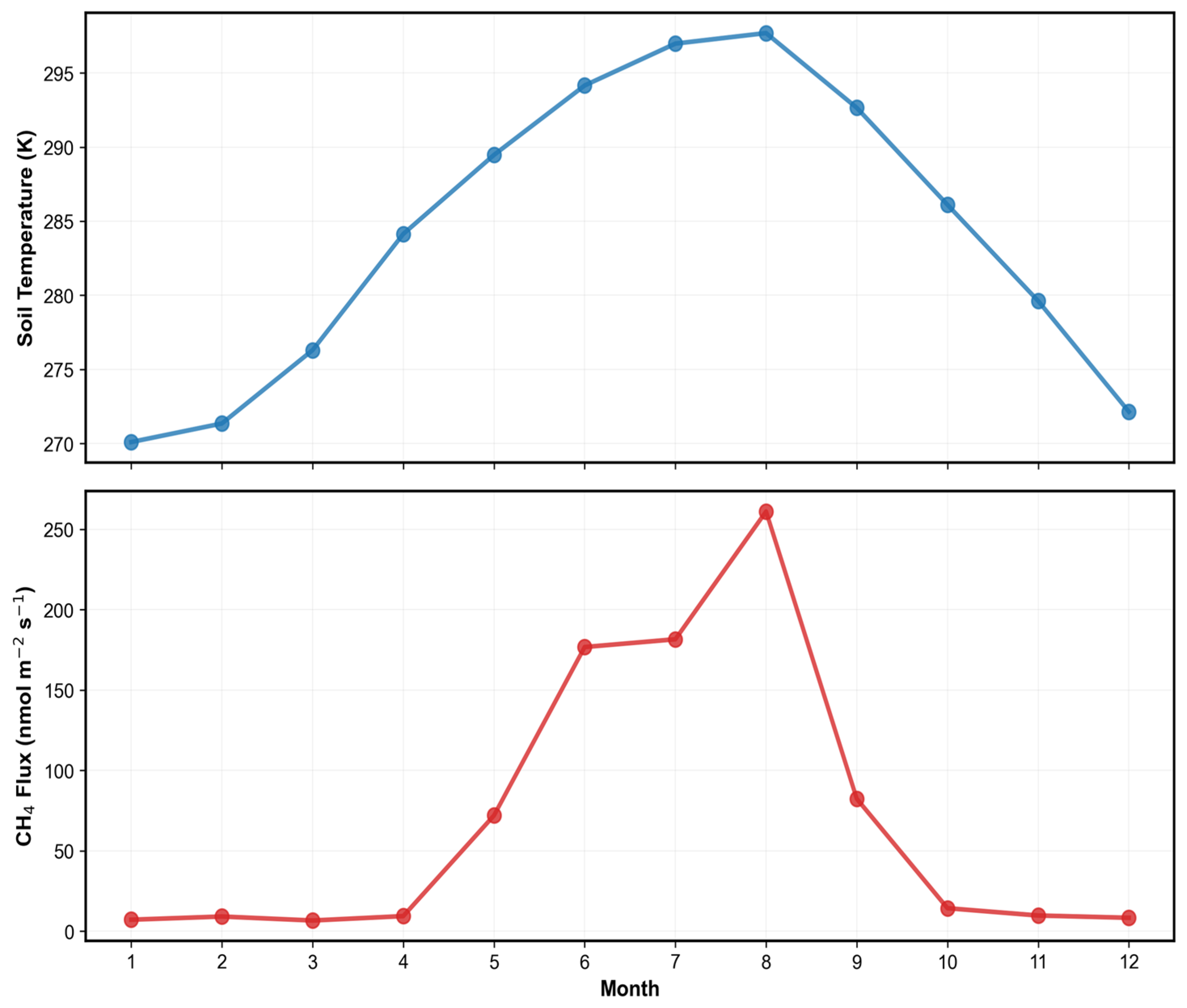
Analysis of the daily model’s results reveals that the temperature-dominated structure of monthly mean CH4 flux is rooted in the strong seasonal coupling between ST and observed CH4 flux. This dominance arises because actual emissions closely mirror the seasonal trajectory of ST. Both variables increase concurrently from May, peak during July and August, and decline sharply after September. This synchronicity confirms, in alignment with previous studies, that seasonal variability in rice paddy methane emissions is primarily driven by temperature-dependent methanogenesis [31,32].
Beyond temperature, emissions are influenced by vegetation development and flooding dynamics; however, as these processes remain relatively stable at the daily scale, ST retains exceptional explanatory power. This robust coupling also offers critical implications for predicting emissions under climate change scenarios. Global warming-induced temperature increases [33] are likely to elevate soil temperatures during the growing season, thereby accelerating methane production. Furthermore, an extended growing season—characterized by earlier spring warming and delayed autumn cooling—may prolong high-emission windows, ultimately leading to a substantial increase in annual methane budgets (Figure 17).
Figure 17.
Monthly variations and seasonal coupling of ST (top) and methane flux (bottom) at the KR-CRK site. The blue and red lines represent the multi-year monthly means of ST (K) and CH4 flux (nmol CH4 m−2 s−1), respectively. The plots illustrate a high degree of synchrony between the two variables, with both reaching their seasonal peaks during the warm summer months (July–August) and declining concurrently during the fallow period.
4.6. Implications for National-Scale Mapping and Management of Rice Paddy Methane Emissions
The application of the daily model to South Korean rice paddies demonstrated that seasonal emission patterns—closely tied to transplanting, growing, and harvesting stages—were stably reproduced. While prediction deviations during abrupt emission shifts represent a source of uncertainty for multi-year estimations, the overall model performance robustly supports the reliability of national-scale spatial assessments. The monthly emission maps clearly revealed strong seasonal periodicity and spatial clustering in response to agricultural practices, as well as hydrological and climatic drivers.
Notably, high-emission areas were concentrated during the peak growing season, when flooded conditions and high temperatures overlap. This aligns with existing literature highlighting plant-mediated transport as a primary pathway for methane release during this period. These findings distinguish between regions and periods of negligible versus concentrated emissions, visually confirming that the growing season is the primary determinant of annual totals in inventory assessments. Consequently, the gridded maps produced in this study serve as a valuable tool for identifying emission hotspots and prioritizing management areas. Furthermore, they provide a scientific basis for selecting optimal periods and regions to implement mitigation strategies, such as alternate wetting and drying (AWD), consistent with previously reported methane reduction potentials [34].
4.7. Limitations
We acknowledge that the US-HRC site provides CH4 flux observations limited to the summer period, and that independent in situ flux measurements across multiple rice-growing regions in South Korea are currently scarce. These constraints limit direct experimental validation of winter emissions and region-specific generalization within South Korea. Expanding long-term flux observations across diverse Korean rice systems, including winter periods, will be essential for further evaluation and for improving national-scale methane emission estimates in future studies. Nevertheless, a single tower may not fully capture sub-grid heterogeneity within a 500 m pixel, and this potential scaling uncertainty should be considered when interpreting gridded emission estimates.
Although the AutoML framework (FLAML) inherently controls model complexity through cross-validation–based model selection and hyperparameter optimization, further improvements in temporal generalization may be achieved through additional regularization strategies and feature engineering. Future work will explore approaches such as temporal feature augmentation (e.g., lagged predictors), site-aware weighting, and regularized ensemble configurations to enhance robustness under anomalous interannual conditions.
4.8. Future Work
As a direct extension of this study, we plan to expand the current AutoML-based framework to other Asian rice-growing regions, with Japan as the primary candidate for immediate application. This geographic expansion aims to address the reviewer’s recommendation to enhance the model’s regional representativeness and mechanistic generalizability across diverse Asian ecosystems. The proposed future research will follow a structured five-step procedure:
- Data Collection and Quality Control
First, we will utilize in situ methane flux observations from the JP-Mse site, which is already part of the FLUXNET-CH4 Community Product. To ensure data reliability, the same two-stage QC procedure developed in this study—comprising point-level outlier elimination and extreme-day filtering—will be applied to the Japanese flux time series.
- Spatiotemporal Feature Integration
Second, we will harmonize Japan-specific environmental drivers with our existing framework. This involves extracting MODIS-derived vegetation indices (NDVI, NDWI, and GNDWI) via Google Earth Engine to characterize phenology and flooding dynamics, alongside collocating ERA5-Land meteorological variables and HWSD soil properties at the 500 m grid level.
- AutoML Model Development and Validation
Third, separate daily and hourly models will be trained using FLAML framework to capture both seasonal totals and high-frequency episodic events in the Japanese context. The model’s temporal generalizability will be rigorously assessed through LOYO cross-validation.
- Spatial Mapping and Masking
Fourth, we will generate 500 m gridded methane emission maps for Japan. To ensure spatial accuracy, we will integrate high-resolution national land-cover maps of Japan as a masking layer, strictly restricting predictions to active rice cultivation areas and minimizing noise from non-target land types.
- Mechanistic Interpretation (SHAP)
Finally, we will employ SHAP analysis to compare the dominant controls of methane emissions between Korea and Japan. This comparative approach will reveal whether the dominance of soil temperature observed in this study holds true across different regions or if site-specific water management and cropping systems (e.g., single vs. double-season rice) introduce distinct multivariate dependencies.
5. Conclusions
This study developed an AutoML-based framework for estimating CH4 emissions from rice paddies by integrating FLUXNET-CH4 observations, MODIS remote sensing, ERA5-Land reanalysis, and HWSD soil data. Our framework enables multi-temporal estimations—spanning hourly to annual scales—and successfully produced high-resolution (500 m) daily CH4 emission maps for South Korean rice paddies. This approach addresses the limitations of conventional annual or region-based inventories, providing a robust basis for a quantitative re-examination of spatiotemporal emission structures.
The daily model exhibited superior predictive performance and temporal generalization, achieving CC of 0.897 in 5-fold cross-validation and 0.819 in LOYO cross-validation. The hourly model also maintained consistent performance (CC: 0.867 for 5-fold; 0.715 for LOYO), despite the challenges of high short-term variability. Comparative analysis indicated that while the daily resolution is optimal for national-scale mapping due to its computational efficiency and accuracy in reproducing seasonal totals, the hourly resolution offers critical insights into episodic events and diurnal structures, facilitating process-oriented interpretations.
SHAP-based analysis revealed that ST is the primary driver in the daily model, whereas the hourly model showed enhanced multivariate dependence on NDVI, SWVL1, SP, and evaporation. This highlights that the dominant controlling mechanisms can diverge depending on temporal resolution, necessitating careful consideration during model interpretation. Furthermore, the high-resolution maps identified that South Korean rice paddy emissions are spatially concentrated during the flooded growing season (July–August), underscoring water management as a pivotal anthropogenic control. These findings provide empirical evidence to refine national greenhouse gas inventories and support the design of spatially targeted mitigation policies, such as alternate wetting and drying (AWD). Future research should aim to further reduce uncertainty by expanding flux networks and integrating these AutoML approaches with process-based models. To this end, we plan to extend this AutoML-based framework to Japan by integrating in situ flux data from the JP-Mse site with national-scale environmental datasets, providing a comparative basis for understanding methane dynamics across diverse Asian rice ecosystems.
Author Contributions
Conceptualization, J.J. and Y.L.; methodology, J.J. and Y.L.; formal analysis, J.J.; data curation, J.J.; writing—original draft preparation, J.J.; writing—review and editing, S.H.K., M.K., J.C., G.Y. and Y.L.; supervision, Y.L. All authors have read and agreed to the published version of the manuscript.
Funding
This work was supported by Korea Environment Industry & Technology Institute (KEITI) through Research and Development on the Technology for Securing the Water Resources Stability in Response to Future Change Project, funded by Korea Ministry of Climate, Energy and Environment (MCEE) (RS-2024-00332300).
Data Availability Statement
All data supporting the findings of this study are available from the corresponding author upon reasonable request.
Conflicts of Interest
The authors declare no conflicts of interest.
Abbreviations
The following abbreviations are used in this manuscript:
| AutoML | Automated Machine Learning |
| CC | Correlation Coefficient |
| CH4 | Methane |
| CV | Cross-Validation |
| ECMWF | European Centre for Medium-Range Weather Forecasts |
| ERA5-Land | ECMWF Reanalysis v5 for Land |
| E | Evaporation |
| FAO | Food and Agriculture Organization |
| FLAML | Fast and Lightweight AutoML |
| FLUXNET-CH4 | FLUXNET Methane Flux Community Product |
| GEE | Google Earth Engine |
| GHG | Greenhouse Gas |
| GNDWI | Green Normalized Difference Water Index |
| HWSD | Harmonized World Soil Database |
| LOYO | Leave-One-Year-Out |
| MAE | Mean Absolute Error |
| MBE | Mean Bias Error |
| MODIS | Moderate Resolution Imaging Spectroradiometer |
| NDVI | Normalized Difference Vegetation Index |
| NDWI | Normalized Difference Water Index |
| NMI | Normalized Mutual Information |
| nRMSE | Normalized Root Mean Square Error |
| QC | Quality Control |
| RMSE | Root Mean Square Error |
| SHAP | Shapley Additive Explanations |
| SP | Surface Pressure |
| ST | Soil Temperature |
| SWVL1 | Soil Water Volume Layer 1 |
| TP | Total Precipitation |
| WRB4 | World Reference Base for Soil Resources (Version 4) |
References
- Yan, X.; Akiyama, H.; Yagi, K.; Akimoto, H. Global estimations of the inventory and mitigation potential of methane emissions from rice cultivation conducted using the 2006 Intergovernmental Panel on Climate Change Guidelines. Glob. Biogeochem. Cycles 2009, 23, GB2002. [Google Scholar] [CrossRef] [Scilit]
- Saunois, M.; Bousquet, P.; Poulter, B.; Peregon, A.; Ciais, P.; Canadell, J.G.; Dlugokencky, E.J.; Etiope, G.; Bastviken, D.; Houweling, S.; et al. The global methane budget 2000–2017. Earth Syst. Sci. Data 2020, 12, 1561–1623. [Google Scholar] [CrossRef] [Scilit]
- Wassmann, R.; Lantin, R.S.; Neue, H.U.; Buendia, L.V.; Corton, T.M.; Lu, Y. Characterization of methane emissions from rice fields in Asia. III. Mitigation options and future research needs. Nutr. Cycl. Agroecosyst. 2000, 58, 23–36. [Google Scholar] [CrossRef] [Scilit]
- Minamikawa, K.; Sakai, N.; Yagi, K. Methane emission from paddy fields and its mitigation options on a field scale. Microbes Environ. 2006, 21, 135–147. [Google Scholar] [CrossRef] [Scilit]
- Ouyang, Z.; Jackson, R.B.; McNicol, G.; Fluet-Chouinard, E.; Runkle, B.R.K.; Papale, D.; Knox, S.H.; Cooley, S.; Delwiche, K.B.; Feron, S.; et al. Paddy rice methane emissions across Monsoon Asia. Remote Sens. Environ. 2023, 284, 113335. [Google Scholar] [CrossRef] [Scilit]
- Sun, M.; Zhang, Y.; Ma, J.; Yuan, W.; Li, X.; Cheng, X. Satellite data based estimation of methane emissions from rice paddies in the Sanjiang Plain in northeast China. PLoS ONE 2015, 10, e0176765. [Google Scholar] [CrossRef] [Scilit] [PubMed]
- Gwon, H.-S.; Choi, E.-J.; Lee, S.-I.; Lee, H.-S.; Lee, J.M.; Kang, S.-S. Research Review of Methane Emissions from Korean Rice Paddies. J. Clim. Change Res. 2022, 13, 117–134. [Google Scholar] [CrossRef] [Scilit]
- Song, Y.; Song, C.; Choi, S.E.; Kim, J.; Kim, M.; Hwang, W.; Roh, M.; Lee, S.; Lee, W.K. Estimating methane emissions in rice paddies at the parcel level using drone-based time series vegetation indices. Drones 2024, 8, 459. [Google Scholar] [CrossRef] [Scilit]
- Hwang, Y.; Ryu, Y.; Huang, Y.; Kim, J.; Iwata, H.; Kang, M. Comprehensive assessments of carbon dynamics in an intermittently irrigated rice paddy. Agric. For. Meteorol. 2020, 285–286, 107933. [Google Scholar] [CrossRef] [Scilit]
- Choi, S.W.; Kim, J.; Kang, M.S.; Lee, S.H.; Kang, N.G.; Shim, K.M. Estimation and mapping of methane emissions from rice paddies in Korea: Analysis of regional differences and characteristics. Korean J. Agric. For. Meteorol. 2018, 20, 88–100. [Google Scholar] [CrossRef]
- Choi, S.W.; Kim, H.Y.; Kim, Y.W.; Kang, M.S.; Kim, J. Estimation and mapping of methane emission from rice paddies in Gyeonggi-do using the modified water management scaling factor. Korean J. Agric. For. Meteorol. 2016, 18, 320–326. [Google Scholar] [CrossRef] [Scilit]
- Zhang, G.; Xiao, X.; Dong, J.; Xin, F.; Zhang, Y.; Qin, Y.; Doughty, R.B.; Moore, B., III. Fingerprint of rice paddies in spatiotemporal dynamics of atmospheric methane concentration in monsoon Asia. Nat. Commun. 2020, 11, 554. [Google Scholar] [CrossRef] [Scilit]
- Knox, S.H.; Jackson, R.B.; Poulter, B.; McNicol, G.; Fluet-Chouinard, E.; Zhang, Z.; Hugelius, G.; Bousquet, P.; Canadell, J.G.; Saunois, M.; et al. FLUXNET-CH4 synthesis activity: Objectives, observations, and future directions. Bull. Am. Meteorol. Soc. 2019, 100, 2607–2632. [Google Scholar] [CrossRef] [Scilit]
- FLUXNET-CH4 Community Product. FLUXNET-CH4 Version 1.0. Available online: https://fluxnet.org/data/fluxnet-ch4-community-product/ (accessed on 15 December 2025).
- Alberto, M.C.R.; Wassmann, R.; Buresh, R.J.; Quilty, J.R.; Correa, T.Q.; Sandro, J.M.; Centeno, C.A.R. Measuring methane flux from irrigated rice fields by eddy covariance method using open-path gas analyzer. Field Crops Res. 2014, 160, 12–21. [Google Scholar] [CrossRef] [Scilit]
- Centeno, C.A.R.; Alberto, M.C.R.; Wassmann, R.; Bicaldo, I.L.; Correa, T.Q. Assessing diel variation of CH4 flux from rice paddies through temperature patterns. Atmos. Environ. 2017, 167, 190–201. [Google Scholar] [CrossRef] [Scilit]
- Vermote, E.; Wolfe, R. MODIS/Terra Surface Reflectance Daily L2G Global 1 km and 500 m SIN Grid V061 (MOD09GA) [Data Set]; NASA Land Processes Distributed Active Archive Center (LP DAAC): Sioux Falls, SD, USA, 2021. [Google Scholar] [CrossRef]
- Gao, B.-C. NDWI—A normalized difference water index for remote sensing of vegetation liquid water from space. Remote Sens. Environ. 1996, 58, 257–266. [Google Scholar] [CrossRef] [Scilit]
- Xiao, X.; Boles, S.; Frolking, S.; Li, C.; Babu, J.Y.; Salas, W.; Moore, B., III. Mapping paddy rice agriculture in South and Southeast Asia using multi-temporal MODIS images. Remote Sens. Environ. 2006, 100, 95–113. [Google Scholar] [CrossRef] [Scilit]
- Muñoz-Sabater, J.; Dutra, E.; Agustí-Panareda, A.; Albergel, C.; Arduini, G.; Balsamo, G.; Boussetta, S.; Choulga, M.; Harrigan, S.; Hersbach, H.; et al. ERA5-Land: A state-of-the-art global reanalysis dataset for land applications. Earth Syst. Sci. Data 2021, 13, 4349–4383. [Google Scholar] [CrossRef] [Scilit]
- FAO; IIASA; ISRIC; ISSCAS; JRC. Harmonized World Soil Database (Version 1.2); FAO: Rome, Italy; IIASA: Laxenburg, Austria, 2012. [Google Scholar]
- Kim, G.-Y.; Jeong, H.-C.; Ju, O.-J.; Kim, H.-K.; Park, J.-H.; Gwon, H.-S.; Kim, P.-J. Establishment of baseline emission factor of methane in Korean rice paddy soil. Korean J. Environ. Agric. 2013, 32, 359–365. [Google Scholar] [CrossRef] [Scilit]
- Hwang, W.; Kim, C.; Cho, K.; Hyun, S.J. Characteristics of greenhouse gas emissions from rice paddy fields in South Korea under climate change scenario RCP-8.5 using the DNDC model. Pedosphere 2021, 31, 332–341. [Google Scholar] [CrossRef] [Scilit]
- Hatala, J.A.; Detto, M.; Baldocchi, D.D. Gross ecosystem photosynthesis causes a diurnal pattern in methane emission from rice. Geophys. Res. Lett. 2012, 39, L06409. [Google Scholar] [CrossRef] [Scilit]
- Roberts, D.R.; Bahn, V.; Ciuti, S.; Boyce, M.S.; Elith, J.; Guillera-Arroita, G.; Hauenstein, S.; Lahoz-Monfort, J.J.; Schröder, B.; Thuiller, W.; et al. Cross-validation strategies for data with temporal, spatial, hierarchical, or phylogenetic structure. Ecography 2017, 40, 913–929. [Google Scholar] [CrossRef] [Scilit]
- Moriasi, D.N.; Arnold, J.G.; Van Liew, M.W.; Bingner, R.L.; Harmel, R.D.; Veith, T.L. Model evaluation guidelines for systematic quantification of accuracy in watershed simulations. Trans. ASABE 2007, 50, 885–900. [Google Scholar] [CrossRef] [Scilit]
- Willmott, C.J.; Matsuura, K. Advantages of the mean absolute error (MAE) over the root mean square error (RMSE) in assessing average model performance. Clim. Res. 2005, 30, 79–82. [Google Scholar] [CrossRef] [Scilit]
- Chai, T.; Draxler, R.R. Root mean square error (RMSE) or mean absolute error (MAE)?—Arguments against avoiding RMSE in the literature. Geosci. Model Dev. 2014, 7, 1247–1250. [Google Scholar] [CrossRef] [Scilit]
- Lundberg, S.M.; Lee, S.-I. A unified approach to interpreting model predictions. In Proceedings of the Advances in Neural Information Processing Systems 30 (NIPS 2017), Long Beach, CA, USA, 4–9 December 2017; pp. 4765–4774. [Google Scholar]
- Hosono, T.; Nouchi, I. The dependence of methane transport in rice plants on the root zone temperature. Plant Soil 1997, 191, 233–240. [Google Scholar] [CrossRef] [Scilit]
- Conrad, R. Microbial ecology of methanogens and methanotrophs. Adv. Agron. 2007, 96, 1–63. [Google Scholar] [CrossRef] [Scilit]
- Yvon-Durocher, G.; Allen, A.P.; Bastviken, D.; Conrad, R.; Gudasz, C.; St-Pierre, A.; Thanh-Duc, N.; del Giorgio, P.A. Methane fluxes show consistent temperature dependence across microbial to ecosystem scales. Nature 2014, 507, 488–491. [Google Scholar] [CrossRef] [Scilit]
- IPCC. Climate Change 2021: The Physical Science Basis; Masson-Delmotte, V., Zhai, P., Pirani, A., Connors, S.L., Péan, C., Berger, S., Caud, N., Chen, Y., Goldfarb, L., Gomis, M.I., et al., Eds.; Contribution of Working Group I to the Sixth Assessment Report of the Intergovernmental Panel on Climate Change; Cambridge University Press: Cambridge, UK; New York, NY, USA, 2021. [Google Scholar]
- Nelson, A.; Wassmann, R.; Sander, B.O.; Palao, L.K. Climate-determined suitability of the water-saving technology “alternate wetting and drying” in rice systems: A scalable methodology demonstrated for a province in the Philippines. PLoS ONE 2015, 10, e0145268. [Google Scholar] [CrossRef] [Scilit]

Disclaimer/Publisher’s Note: The statements, opinions and data contained in all publications are solely those of the individual author(s) and contributor(s) and not of MDPI and/or the editor(s). MDPI and/or the editor(s) disclaim responsibility for any injury to people or property resulting from any ideas, methods, instructions or products referred to in the content. |
© 2026 by the authors. Licensee MDPI, Basel, Switzerland. This article is an open access article distributed under the terms and conditions of the Creative Commons Attribution (CC BY) license.