A Multimodal Feature Fusion Framework for UAV Positioning in Weak GNSS Environments Using a Priori High-Resolution Satellite Imagery

Highlights

What are the main findings?

• This paper proposes a real-time UAV positioning framework for weak GNSS environments, which establishes high-precision cross-modal alignment between drone and satellite imagery via a “Multimodal features + LightGlue” strategy.
• A synergistic point-line-plane feature fusion module is designed to provide robust geometric constraints, effectively mitigating the feature sparsity and matching failures common in low-texture and high-dynamic scenarios.

What are the implications of the main findings?

• The shift from GNSS-dependency to a robust multimodal geometric fusion paradigm offers a mission-critical solution for UAV autonomy, ensuring high-precision positioning continuity and operational security in GNSS-denied environments.
• The systematic analysis of how altitude, scale, and seasonal dynamics influence performance reveals that future robust positioning architectures should prioritize adaptive feature selection to ensure operational stability under variable deployment conditions.

Abstract

To address the challenges of unmanned aerial vehicle (UAV) navigation in weak global navigation satellite system (GNSS) environments, this study proposes a novel multimodal feature fusion framework for real-time positioning using a priori high-resolution satellite imagery. This framework utilizes georeferenced satellite images as matching sources and employs a “Multimodal features + LightGlue” algorithm to achieve high-precision cross-modal matching. By combining point, line, and plane features for enhanced robustness in low-texture scenarios, the system further integrates LightGlue’s lightweight confidence classifier to accelerate inference while maintaining high accuracy on challenging image pairs. Consequently, the proposed method outperforms LoFTR, RoMa, SuperPoint + SuperGlue, and SuperPoint + LightGlue in matching performance. Experimental results demonstrate that at a flight altitude of 80 m, the average real-time positioning error is 0.73 m, which increases to 6.24 m at 480 m. Factors such as ground object type, seasonal changes, flight altitude, and satellite image scale significantly influence accuracy. This research demonstrates that the visual navigation system meets practical operational needs for real-time UAV positioning in GNSS-deprived environments.

1. Introduction

UAVs have a long history of technological development, evolving from their initial roles as training aids and target drones to versatile platforms capable of tasks such as target search, information reconnaissance, and disaster relief [1,2]. Therefore, the autonomous positioning and navigation system, as one of the most important components of UAVs, has gradually become the focus topic in this research field. At present, the main navigation technologies of UAVs include the global navigation satellite system (GNSS), inertial navigation system (INS), computer vision navigation system, etc. [3,4]. However, in weak GNSS environments, such as mountain terrain occlusion, geomagnetic interference, and even fierce electronic warfare or electromagnetic interference, the GNSS signal that UAV navigation mainly depends on is interfered with, which may lead to large deviations in UAV self-positioning, making UAVs inoperable or unstable, and even threatening the safety of operators and other people’s lives and property [5,6]. The inertial navigation system has high short-term accuracy, but errors will gradually accumulate over time, which cannot meet the flight mission of UAVs with highly dynamic and long-time flight [7,8,9].

In order to ensure the navigation and positioning accuracy of UAVs in weak GNSS environments, visual navigation schemes might fill the gaps in GNSS and improve the navigation accuracy of UAVs [10,11,12,13,14]. Computer vision navigation is a navigation technology that uses visual sensors to perceive external environmental information as the basis for drone flight [15,16,17].

In 2007, Trawny et al. proposed an estimation algorithm that integrated inertial and visual measurements to study the pose estimation of spacecraft during planetary surface descent in order to achieve fixed-point landing [18]. In 2009, Conte et al. proposed a drone navigation system based on aerial image registration to explore the possibility of using geographic reference satellite images or aerial images to assist drone navigation and positioning in the event of GNSS failure [19]. In 2012, Lee et al. replaced the inertial navigation system with a monocular vision system and proposed a vision-based TRN system [20]. They estimated relative plane motion using ground features and combined the translation information obtained by the vision system with the measured terrain height to achieve a vision-based autonomous navigation system for UAVs. In 2015, Dumble et al. proposed an effective terrain-assisted navigation method, which also matched the terrain information in the drone view with existing terrain databases to achieve drone positioning [21]. In 2021, Mughal used drone onboard cameras and pre-stored geographic reference images for drone localization, proposing a deep learning framework to extract features from drone images. These features were matched with pre-prepared images with geographic markers to complete the drone localization work [22]. In 2022, Sui et al. proposed a fast two-stage matching method without detectors to improve the visual positioning algorithm of low-altitude drones. They used feature point matching and perspective transformation modules in both coarse and fine matching stages to improve the visual positioning accuracy of low-altitude drones. The average positioning accuracy of this method was 2.24 m [23]. In 2023, Wu et al. proposed a new hierarchical visual localization method based on graph neural networks to learn the intrinsic connections of feature points and improve matching accuracy. Finally, the absolute coordinates of the drone were calculated, with an average localization error of 10.8 m [24]. In 2024, Liu et al. proposed a deep learning-based framework for airport runway line detection and the fusion of visual information with IMU data to achieve robust UAV landing localization [25]. In 2025, Tong et al. introduced a robust top-view absolute positioning method (RTAPM) that integrated point-line feature matching with visual-inertial joint optimization to ensure reliable UAV navigation in GNSS-denied environments [26].

However, high precision UAV visual navigation is still challenging due to low matching accuracy, high time complexity, and poor performance, especially in large-scale, low-texture areas in the field, where the matching effect cannot meet the needs of a wide range of drone applications [27]. It should be noted that the ‘time complexity’ mentioned here primarily refers to the online inference performance during flight rather than the offline training phase. Therefore, high-accuracy and fast image matching algorithms are crucial for vision-based autonomous navigation of UAVs.

Common feature matching algorithms include scale-invariant feature transform (SIFT) [28], speeded-up robust feature (SURF) [29], features from accelerated segment test (FAST) [30], oriented FAST and rotating BRIEF (ORB) [31], binary robust invariant scalable keypoints (BRISK) [32], etc. Although these classic feature extraction methods have strong interpretability in theory, their robustness is not strong and they are easily affected by uncertain factors, such as sun lighting and occlusion. For matching between images with excessive perspective changes, incorrect matching often occurs due to large differences between images. With the advancement of computer computing power and the emergence of large, labeled datasets, deep learning has gradually become an increasingly mainstream means of solving problems in the field of computer vision.

The SuperPoint algorithm proposed in 2018 trained a network for extracting image features and feature descriptors using self-supervision, but its performance in actual matching was not satisfactory, which also reflects the shortcomings of SuperPoint in self-supervised training [33]. In 2020, based on the SuperPoint algorithm, the SuperGlue algorithm was proposed. SuperGlue is a feature matching algorithm based on graph convolutional neural networks, which uses key point encoding, a multi-head attention mechanism, optimal transmission optimization allocation, and other main technologies to construct a learnable feature matching machine. The key points and descriptors are calculated using SuperPoint, and the best matching key points are obtained through this matching machine [34]. Compared with traditional feature matching algorithms, it solves the problem of insufficient texture features or local features not being representative, which leads to ineffective feature matching. The LoFTR algorithm proposed in 2021 uses a self-attention layer and cross-attention layer in the transformer to obtain feature descriptors based on two images, enabling the algorithm to generate dense matching in low-texture areas [35]. In 2024, RoMa was developed by Parskatt, which is an open-source dense feature matching algorithm that performs pixel-level dense feature matching, estimates dense transformations between image pairs, and provides reliable matching confidence [36]. In 2023, LightGlue improved upon SuperGlue by retaining its multi-head attention mechanism and introducing a lightweight confidence classifier that achieved faster inference speed and lower computational complexity on easily matched image pairs, while still maintaining high accuracy on challenging image pairs [37]. In 2025, Wang et al. demonstrated that the combination of SuperPoint and LightGlue achieved optimal performance in challenging large-angle scenarios, yielding approximately ten times more matches than traditional SIFT through its adaptive pruning and robust matching mechanisms [38].

Despite recent advancements, existing UAV visual positioning methods still face several limitations: (1) a high reliance on single-point features, which often leads to matching failures in low-texture or repetitive urban environments; (2) significant modal gaps and perspective differences between UAV and satellite imagery that traditional descriptors struggle to bridge; and (3) the inefficient utilization of structural geometric information, such as lines and planes, which are abundant in urban scenes.

To address these issues, the innovations of this study are as follows:

(1) A synergistic point-line-plane feature fusion strategy is proposed to provide multi-level geometric constraints, significantly enhancing matching robustness in complex environments.

(2) A high-precision cross-modal alignment method is developed by optimizing the LightGlue framework, leveraging its graph-based attention mechanism to handle the domain gap between drone and satellite imagery.

(3) A robust UAV positioning framework specifically for weak GNSS environments is established, achieving reliable absolute localization through the integration of multimodal features and prior satellite information.

Building upon these improvements, we propose a novel multimodal features fusion framework that integrates point, line, and plane features for real-time UAV positioning in weak GNSS environments. The framework utilizes geo-referenced high-resolution satellite imagery as the database. During operation, UAV images are captured via an onboard monocular camera and a multimodal feature-based LightGlue algorithm is employed for robust cross-modal matching. Finally, the drone’s absolute coordinates are determined through a dedicated positioning algorithm to ensure reliable navigation in GNSS-denied scenarios.

2. Methodology

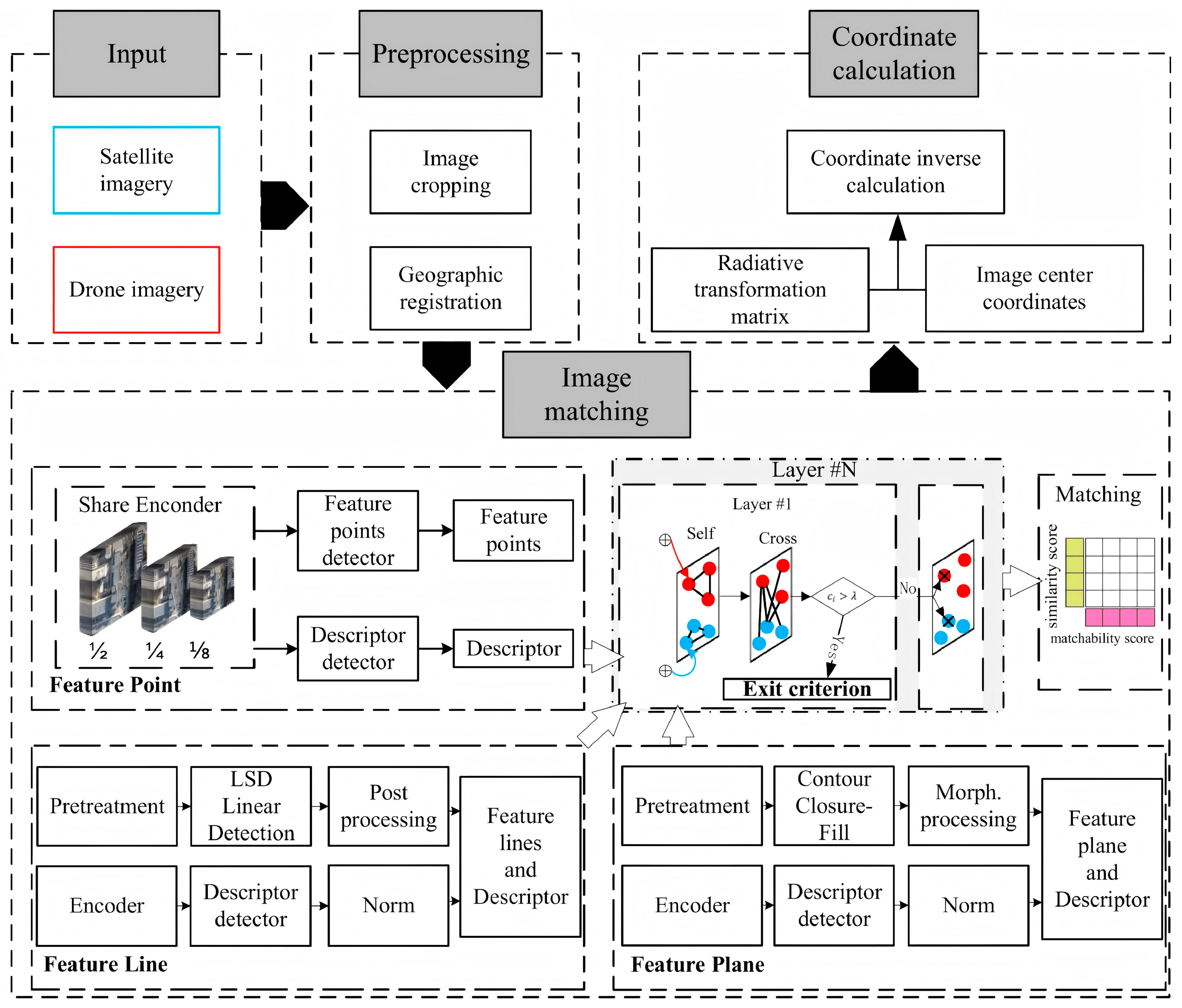
In this study, satellite orthorectified optical images containing geographic information are matched with real-time optical images collected by drones to calculate the real-time position of the drones. Therefore, the matching effect greatly affects the accuracy of the calculated drone coordinates. We use the LightGlue image matching algorithm based on multimodal features method to complete the most important image matching work. The algorithm flow for real-time UAV positioning is shown in Figure 1. First, the input images are preprocessed, including orthorectified, radiometric, and georegistered satellite optical images, as well as orthorectified and radiometric corrected drone images. Then, the images to be matched are input and the SuperPoint algorithm is used to extract the feature points and descriptors of the images to be matched. Compared with other feature extraction algorithms, the SuperPoint algorithm uses a shared encoder that adopts a network structure similar to VGG to reduce the size of the input image. This not only calculates pixel-level feature points and feature descriptors simultaneously in one forward propagation but also greatly improves model efficiency and performance by reducing image dimensionality. In addition, feature lines are extracted via a Line Segment Detector (LSD), and feature planes are delineated through edge detection and closed-contour analysis. Crucially, the descriptors for these feature lines and planes are calculated following the SuperPoint paradigm. By leveraging the shared convolutional backbone, all multimodal primitives are derived from a common semantic basis—specifically, the dense feature tensor generated before the final spatial sampling. This ensures that complex geometric structures are effectively converted into high-dimensional semantic tokens. Through a standardized pipeline of bicubic interpolation and L2 normalization, these multimodal features are homogenized into unit-length vectors, achieving intrinsic mathematical alignment.

Next, the extracted multimodal features and descriptors are input into the LightGlue network. The LightGlue network proposes a self-attention mechanism and a cross-attention mechanism to extract fusion information between feature points within the same image and visual correlation information between feature points between two images. By actively searching for context, the feature point specificity is increased, which can eliminate some singular matches and ultimately obtain the matching relationship of image features. In addition, LightGlue has added a lightweight confidence classifier to help determine whether to stop the inference process. If only a few points have high confidence, the inference process continues to the next layer, but unmatched points with low confidence are removed. This approach can achieve faster inference speed on easily matched image pairs while still maintaining accuracy on challenging image pairs. Finally, coordinate calculation is performed to obtain the affine transformation matrix of the two images in two-dimensional space through the correspondence between the same named points of the two images to be matched. Because the drone image is captured vertically by the drone, the center position of the drone-captured image is the location of the drone. By using satellite images with geographic information and affine transformation matrices to calculate the center position of the drone image, the plane coordinates of the drone can be obtained.

2.1. SuperPoint Network

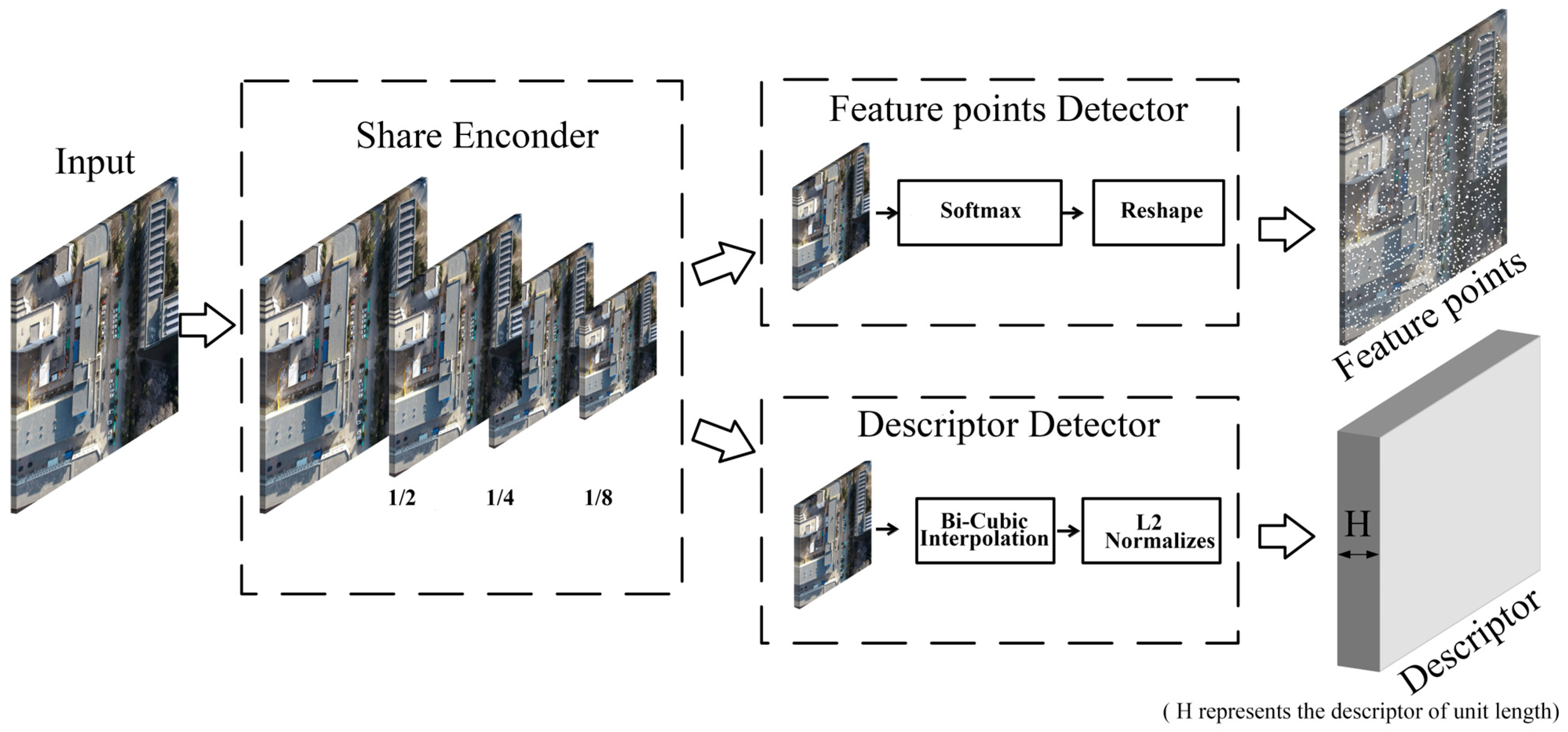
SuperPoint is a self-supervised training network framework for extracting feature points and computing descriptors, which does not require manual labeling of data but continuously improves performance through self-iteration. Compared with traditional neural networks, SuperPoint uses a fully convolutional model to process full-size images, and the feature point and descriptor extraction part uses a shared encoder, which can simultaneously calculate pixel-level feature points and feature descriptors in one forward propagation, improving model efficiency and performance. The SuperPoint network structure diagram is shown in Figure 2.

2.1.1. Share Encoder

Previous methods typically required two feedforward propagations, with feature points and descriptors calculated separately and lacking sharing. However, SuperPoint networks solved this problem by using a shared encoder. The SuperPoint network first uses a VGG-style encoder to reduce the dimensionality of the image and extract features in order to reduce the computational complexity of the subsequent network and improve performance.

2.1.2. Feature Points Detector

The feature point detection network essentially calculates the probability of each pixel becoming a feature point. Among them, a Dustbin channel is added to the input network for output when there are no feature points in the local area. The Dustbin channel can avoid generating a relatively large-value output in the 64-dimensional features of Softmax when there are no feature points in the image, forming noise points that affect the final result.

2.1.3. Point Descriptor Detector

The extraction of feature descriptors is similar to feature point extraction, which also inputs the image output from the encoder. The feature map output through convolution is then subjected to the Bi Cubic Interpolation and L2 Normalization algorithms to obtain descriptors of unit length.

2.1.4. Loss Function

The final loss is the sum of two intermediate losses, one is feature point detection and the other is descriptor computation, which can optimize both losses of a pair of images simultaneously.

$$\mathcal{L}\left(\mathcal{X},{\mathcal{X}}^{\prime },\mathcal{D},{\mathcal{D}}^{\prime };Y,Y^{\prime },S\right)={\mathcal{L}}_p\left(\mathcal{X},Y\right)+{\mathcal{L}}_p\left({\mathcal{X}}^{\prime },Y^{\prime }\right)+\lambda {\mathcal{L}}_d\left(\mathcal{D},{\mathcal{D}}^{\prime },S\right)$$

(1)

The final inputs are $\mathcal{X}, {\mathcal{X}}^{\prime }, \mathcal{D}, {\mathcal{D}}^{\prime }, Y, Y^{\prime }, \mathrm{a}\mathrm{n}\mathrm{d} S$, where $\mathcal{X}$ is the input feature point, $Y$ is the feature point label, $\mathcal{D}$ is the output feature descriptor, and $S$ is the correspondence of feature points. In addition, $\lambda$ is used here to balance the loss relationship between the feature point detection network and the descriptor computing network.

The feature point correlation loss ${\mathcal{L}}_p$ defines a cross-entropy loss:

$${\mathcal{L}}_p\left(\mathcal{X},Y\right)={\displaystyle \frac{1}{H_c{W}_c}}{\sum }_{h=1w=1}^{H_c{,W}_c}{l}_p\left(x_{hw};y_{hw}\right)$$

(2)

wherein

$$l_p\left(x_{hw};y_{hw}\right)=-\mathit{log}\left({\displaystyle \frac{\mathit{exp}\left(x_{hw}\right)}{{\sum }_{k=1}^{65}\mathit{exp}\left(x_{hw}\right)}}\right)$$

(3)

Among them, $H_c=H/8$, $W_c=W/8$, where $y_{hw}$ is the true value, that is, the pixel in the 8 × 8 grid that is the feature point; and $x_{hw}$ is a feature vector with a length of 65, and each value of the vector represents the response value of the corresponding feature point on the pixel.

The eigenvector related loss ${\mathcal{L}}_d$ is defined as a hinge loss:

$${\mathcal{L}}_d\left(\mathcal{D},{\mathcal{D}}^{\prime },S\right)={\displaystyle \frac{1}{{\left(H_c{W}_c\right)}^2}}{\sum }_{h=1w=1}^{H_c{,W}_c}{\sum }_{h^{\prime }=1w^{\prime }=1}^{H_c{,W}_c}{l}_d\left(d_{hw},{d^{\prime }}_{h^{\prime }{w}^{\prime }};s_{hw{h}^{\prime }{w}^{\prime }}\right)$$

(4)

wherein

$$l_d\left(d_{hw},{d^{\prime }}_{h^{\prime }{w}^{\prime }};s_{hw{h}^{\prime }{w}^{\prime }}\right)={\lambda }_d\times s\times max\left(0,m_p-d^T{d}^{\prime }\right)+\left(1-s\right)\times max\left(0,d^T{d}^{\prime }-m_n\right)$$

(5)

Among them, ${\lambda }_d$ is the defined weight, and $s$ (representing $s_{hw{h}^{\prime }{w}^{\prime }}$) is a function that determines whether it is the same feature point through homography matrix correlation:

$$s_{hw{h}^{\prime }{w}^{\prime }}=\left\{\begin{array}{c}1, if‖\widehat{\mathcal{H}{p}_{hw}}-p_{h^{\prime }{w}^{\prime }}‖\le 8\\ 0, otherwise\end{array}\right.$$

(6)

where $p_{hw}$ is the center point of an 8 × 8 grid. When the distance between $\widehat{\mathcal{H}{p}_{hw}}$ and $p_{h^{\prime }{w}^{\prime }}$ is less than 8 pixels, the matching is considered successful. In addition, when the matching is successful, a penalty will be imposed when the similarity $d^T{d}^{\prime }$ is greater than the positive sample threshold $m_p$. When matching fails, a penalty will be imposed when the similarity $d^T{d}^{\prime }$ is less than the negative sample threshold $m_p$. So, when matching is successful, the similarity should be high, and when matching fails, the similarity should be low.

2.2. Feature Line Extraction

Feature line extraction accurately extracts representative line or edge features from images and is widely used in target recognition, image registration, 3D reconstruction, motion analysis, and industrial quality inspection scenarios. Line features provide long-range geometric constraints in weakly textured areas of an image by detecting continuous edge structures such as building contours and road boundaries. The line feature extraction method used in this paper is mainly based on LSD (Line Segment Detector).

2.2.1. Line Segment Detector

Line Segment Detector (LSD) is a line segment detection algorithm used in computer vision. It is a method for extracting lines and segments from images that is characterized by high efficiency, robustness, and scalability. The core idea of the LSD method is to merge pixels with similar gradient directions to form line features. Firstly, Gaussian filtering is used to smooth the input image and remove the influence of noise. The gradient magnitude and level-line angle of each pixel are then calculated to capture the local orientation and intensity variations. Subsequently, by integrating similar pixels in the image gradient field, line support regions (LSRs) are formed. For each line segment support domain, there may be a feature line inside. By calculating whether the main direction and gradient direction of pixels in the support domain meet the set threshold angle, it is determined whether there is a feature line based on the proportion of pixels in the domain that meet the threshold condition. Finally, the possible line features detected are pixel-merged to obtain the line feature detection result.

The LSD algorithm is an excellent method for extracting line segments, which can provide feature descriptions for weakly textured areas in images by adding LSD-extracted line features. However, in practical use, LSD extraction of line segments is prone to detecting many outliers, resulting in a large number of invalid short line features. Invalid short lines have little reference value for subsequent image matching, and a large number of short lines will increase computational costs and affect the real-time performance of the algorithm. In addition, some feature lines may be the same straight line.

In response to the problems of excessive ineffective short lines and broken lines in LSD, this paper adopts a strategy of length constraint and short line merging on the original line features extracted by LSD. For the line features extracted by LSD, the normalized coordinates corresponding to endpoints $l_A$ and $l_B$ are $l_A=(x_1,y_1)$ and $l_B=(x_2,y_2)$, respectively. The length is calculated using the distance formula.

By setting a threshold, line segments with a length less than the threshold are removed. After length constraint, invalid short lines are removed, but there are cases where feature lines are broken. By merging these broken line features into long line features, more effective line features can be extracted and algorithm accuracy can be improved.

In response to the limitation of the LSD algorithm, two short lines that are judged to be the same line are merged by using the minimum distance and angle between two line segments as the criteria for judgment. First, the angle difference is calculated between two line segments and line segment pairs with angle differences less than the threshold are retained. Then, the horizontal and vertical distances of the retained line segment combinations are calculated. The line segment pairs with distances that meet the threshold are merged, and merged line segments with better quality are included in subsequent matching to improve the reliability of matching. For the two extracted line segments $l_1$ and $l_2$, its endpoints are $S_1=\left(x_1,y_1\right)$, ${ E}_1=\left(x_2,y_2\right)$ and $S_2=\left(x_3,y_3\right)$, $E_2=(x_4,y_4)$, respectively, and the shorter of the two line segments is set to its length $d$. The angles of line segments $l_1$ and $l_2$ relative to the vertical direction are calculated as ${\theta }_1$ and ${\theta }_2$, respectively. When the angle difference $\Delta \theta$ between two line segments is less than the threshold $M$, further judgment needs to be made by the distance between the two line segments to remove line segments that are parallel but too far apart. For line segments $l_1$ and $l_2$, their horizontal distance is denoted as $S_h$ and vertical distance is denoted as $S_v$. Only when $S_h$ and $S_v$ are less than $d/2$, will $l_1$ and $l_2$ be merged. The calculation formulas for the horizontal distance between two line segments, denoted as $S_h$, and the vertical distance, denoted as $S_v$, are as follows:

$$S_h=min\left(\begin{array}{c}\left|x_1-x_3\right|,\left|x_2-x_3\right|\\ \left|x_1-x_4\right|,\left|x_2-x_4\right|\end{array}\right)$$

(7)

$$S_v=min\left(\begin{array}{c}\left|y_1-y_3\right|,\left|y_2-y_3\right|\\ \left|y_1-y_4\right|,\left|y_2-y_4\right|\end{array}\right)$$

(8)

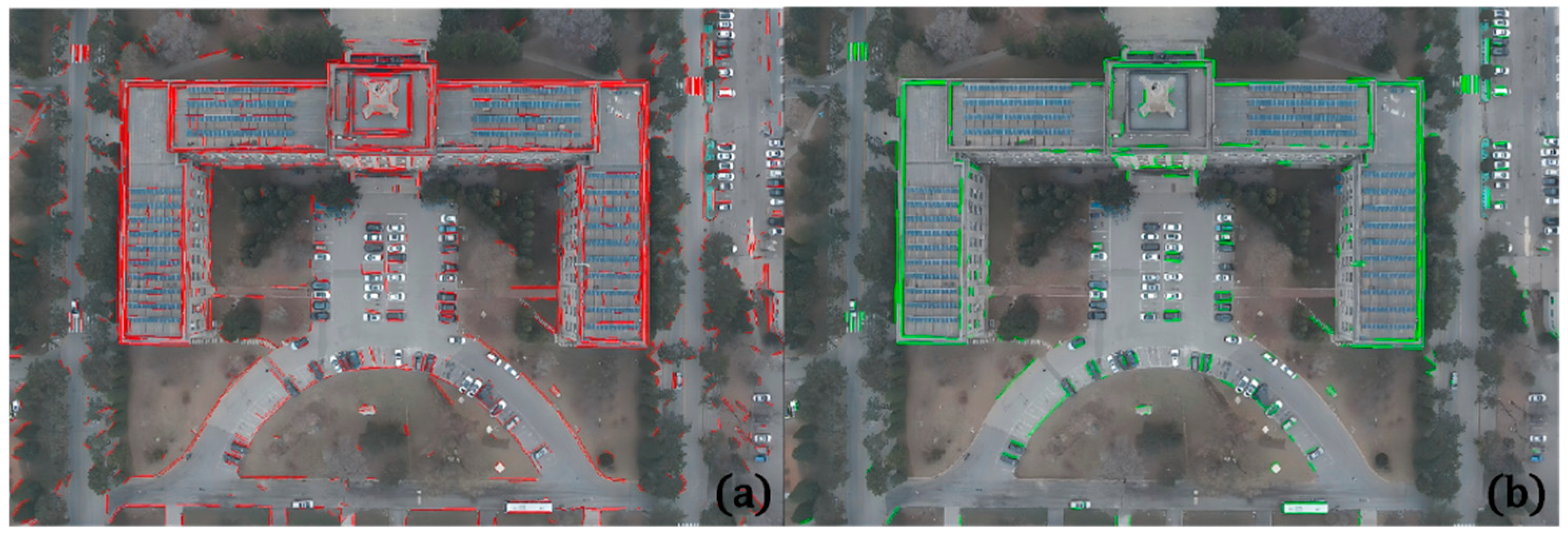
The comparison before and after post-processing of line features is shown in Figure 3. It can be clearly seen from the figure that a large number of discrete line segments are merged into complete structural lines, while reducing cluttered short lines and reducing the number of line segments by 67%.

2.2.2. Line Descriptor Detector

The descriptor calculation for feature lines is designed to be consistent with point-based encoding to facilitate seamless multimodal integration. Initially, the image is processed through a shared convolutional encoder to produce a dense feature tensor generated before the final spatial sampling, which encapsulates fundamental semantic attributes such as spatial, textural, and spectral information. For each detected and merged line segment, a spatial search is conducted on this dense tensor within a 5-pixel proximity of the line’s geometric path. The descriptors of pixels exhibiting the highest saliency response strengths along the segment are sampled through bicubic interpolation and L2 normalization and are subsequently utilized as representative semantic tokens for the feature line in the matching stage. This strategy effectively transforms geometric line structures into high-dimensional tokens that are mathematically aligned with point features.

2.3. Feature Plane Extraction

A feature plane is a closed region with significant semantic or structural features extracted through algorithms in the fields of computer vision and image processing. Its principle is based on techniques such as edge detection, morphological optimization, connected component analysis, and geometric constraint screening. The feature plane utilizes region segmentation techniques to capture the overall structural information of the scene (such as water bodies and vegetation coverage areas), and together with feature points and lines, performs multi-level feature expression on the image. This article extracts feature planes by first using gradient detection methods such as Canny operator to generate edge maps and then using a contour search algorithm to convert continuous edges into closed contours. Then, a morphological closure operation is used to connect broken edges and fill voids, combined with an erosion dilation operation to eliminate noise. Finally, effective regions are selected through connected region labeling and geometric features such as area and perimeter.

2.3.1. Closed Contour Detection

In this paper, the Suzuki algorithm was utilized to detect the closed contour, which can efficiently extract the contours of objects from binary images and determine the nested relationships between these contours. It is widely used in fields such as computer vision and image processing for tasks such as object detection and image segmentation. The algorithm first scans the binary image line by line, starting from the top left corner of the image and traversing each pixel in order from left to right and top to bottom. When encountering an unmarked pixel with a foreground value, it is used as the starting point for a new contour. Let the image be $I(x,y)$, where $x$ is the column coordinate and $y$ is the row coordinate. If $I(x,y)\ne 0$ and has not been marked as visited before, then $(x,y)$ can be used as the starting point.

Starting from the starting point, the next boundary point is searched according to a certain neighborhood rule. Taking the 8-neighborhood as an example, for the current point $\left(x_n,y_n\right)$, the coordinates of its 8-neighborhood points are $\left(x_n+i,y_n+j\right)$, where $i,j\in \left\{-\mathrm{1,0},1\right\}$ and $\left(i,j\right)\ne \left(\mathrm{0,0}\right)$. During the tracking process, the next boundary point is determined by checking whether the neighboring points are non-zero pixels and have not been visited. Assuming the current point is $P_n=\left(x_n,y_n\right)$, and the next point $P_{n+1}=\left(x_{n+1},y_{n+1}\right)$, the search rule can be expressed as follows:

$$\left\{\begin{array}{l}I\left(x_{n+1},y_{n+1}\right)\ne 0\\ \mathit{Point}\left(x_{n+1},y_{n+1}\right) \mathit{is} \mathit{not} \mathit{visited}\end{array}\right.$$

(9)

When the tracking returns to the starting point, the tracking of a contour ends. When $P_m=\left(x_m,y_m\right)$ satisfies $x_m=x_0$ and $y_m=y_0$ (where $\left(x_0,y_0\right)$ is the starting point), a contour extraction is completed.

During the process of tracking contours, passing pixels are marked to avoid duplicate tracking. Meanwhile, a unique identifier is assigned to each contour. In addition, the Suzuki algorithm constructs a hierarchical structure based on the nested relationships between contours. If a contour is completely contained within another contour, the internal contour is called a child contour, and the external contour is called a parent contour. By maintaining a tree structure to represent this hierarchical relationship, each node contains information about the contour as well as pointers to its parent node, child nodes, previous contour, and next contour. The above process is continuously repeated to scan the image until all foreground pixels have been marked or tracked, thereby extracting all contours and their hierarchical structures from the image.

2.3.2. Morphological Post-Processing

Mathematical morphology is a tool for analyzing and processing images based on morphological structural elements. Its basic idea is to use structural elements to explore images, see if the elements of the structure can be well filled into the image, and verify the effectiveness of the method. There are four basic operations in mathematical morphology: dilation, erosion, opening, and closing. When processing binary and grayscale images, they play different roles based on the characteristics of the image.

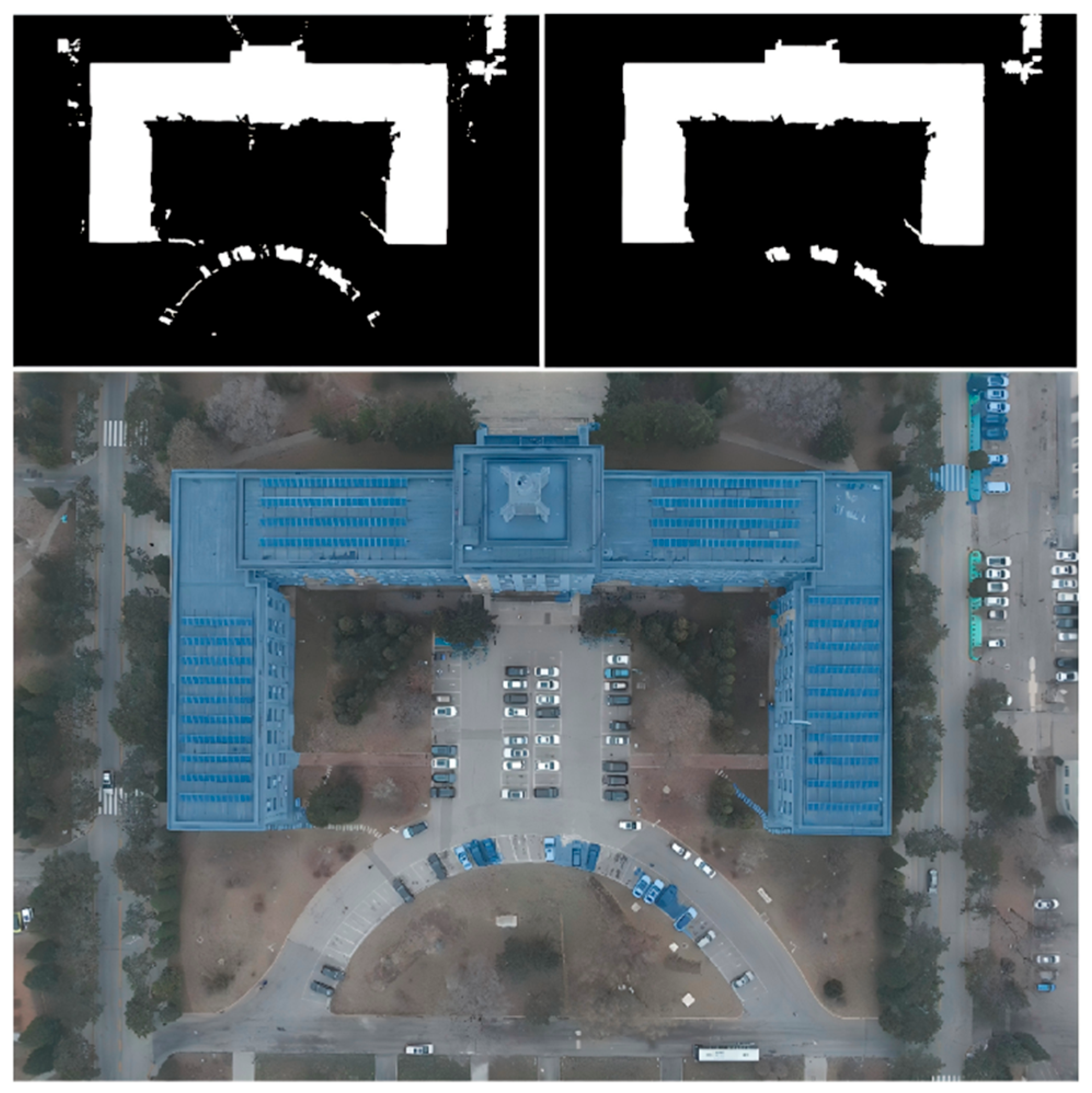
Post-processing is a key step in feature plane extraction, aimed at eliminating noise interference and enhancing contour integrity. The core process includes morphological operations and connected region analysis. Firstly, the extracted contour lines are closed to close disconnected contours caused by occlusion or other reasons. Then, the closed areas are filled to form a preliminary feature plane, as shown in Figure 4. From the figure, it can be seen that the extracted feature plane contains many small noise points and cluttered edge lines. Using the 8-neighborhood Connected Components Labeling (CCL) algorithm, the binary image is segmented into independent regions. Let the labeled image be $L\left(x,y\right)$, the area $A_k$ of each connected region $C_k$ is calculated as follows:

$$A_k={\sum }_{(x,y)\in C_k}L\left(x,y\right)$$

(10)

The effective area is filtered through threshold $A_{min}$, components with an area greater than the threshold are retained, small noise areas are effectively removed, and the semantic integrity of the feature plane is improved.

The feature plane extraction results are shown in Figure 4. Post-processing combines morphological operations with connected region analysis, significantly improving the integrity and noise resistance of the feature plane.

To maintain cross-modal consistency, the feature plane descriptors are extracted using the same shared encoder and the dense feature tensor generated before the final spatial sampling. Based on the segmented plane masks, the framework performs a targeted filtering within the closed boundaries of each plane. Specifically, the descriptors corresponding to pixels with peak saliency scores within mask regions are selected as representative surface tokens. By undergoing the same normalization and interpolation pipeline as the point and line modalities, these surface-based descriptors are projected into the unified semantic space, ensuring that area-level structural information is mathematically aligned and seamlessly integrated with point and line primitives.

2.4. LightGlue Network

LightGlue is a deep learning-based local feature matching method that combines attention mechanisms with adaptive features based on SuperGlue. It can be flexibly adjusted according to the difficulty of the matching problem, achieving faster inference speed on easily matched image pairs while maintaining accuracy on challenging image pairs. It should be noted that while the offline training of graph-based architectures is computationally intensive, the LightGlue framework is specifically optimized for online inference efficiency. By incorporating an adaptive depth mechanism and dynamic sparse message passing to prune unreliable features, the model adaptively adjusts its computational load based on the difficulty of the match, thereby fulfilling the strict real-time requirements for onboard UAV processing. Crucially, the inputs to this network are the homogenized multimodal tokens (points, lines, and surfaces) sampled from the dense feature tensor. This ensures that geometric structures are integrated into the matcher as semantically aligned 256-dimensional vectors. 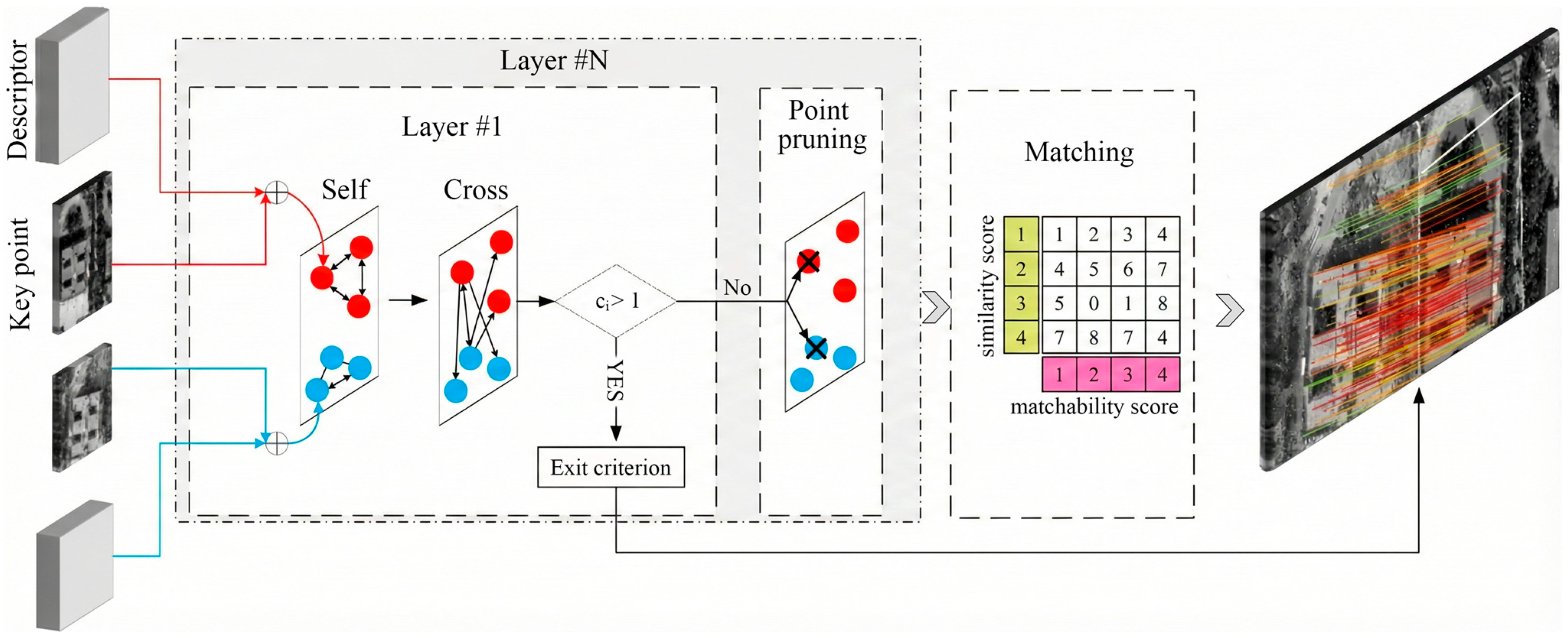The algorithm principle of LightGlue is shown in Figure 5. The main body is composed of a pile of $N$ identical layers, which jointly process two sets of keypoints and descriptors. Each layer consists of self-attention units and cross-attention units that update the representation of each point. Among them, the classifier decides whether to stop reasoning at each layer to avoid unnecessary calculations. Finally, the lightweight matchmaker combines the similarity score and the matchability score to determine whether two points match.

2.4.1. Transformer Backbone

Key points and descriptors from two images are input, with each layer consisting of one self-attention unit and one cross-attention unit, totaling $N$ layers.

• Self-attention: Each point focuses on all points in the same image. For each point $i$, two-dimensional point position $p_i$ normalized by the image size and descriptor $d_i$ are initialized by descriptor $d_i$ to obtain state $x_i$. Current state $x_i$ is decomposed into key vector $k_i$ and query vector $q_i$ through a linear transformation. Rotational encoder $R$ is used to define attention score $a_{ij}$ between points $i$ and $j$ in order to capture their relative positions:

  $$a_{ij}=q_i^{{\rm T}}R\left(p_j-p_i\right)k_i$$

  (11)

  By dividing the space into 1/2 $2D$ subspaces and rotating and projecting them onto learnable basis vectors, position encoding is achieved. Rotational encoding enables the model to retrieve points $j$ with learned relative positions. This encoding is the same in all layers and is only computed once and cached. In our multimodal framework, the self-attention mechanism explicitly models the intra-modal spatial dependencies and geometric topology within each image. Specifically, it characterizes the structural constraints that line and surface primitives impose on the spatial distribution of nearby point features, thereby enhancing the geometric consistency of the local descriptors before matching.
• Cross-attention: Each point in image $I$ will focus on all points in another image $S$. This layer facilitates the dynamic weighted fusion between the UAV and satellite feature sets. By calculating affinity scores across different modalities, the cross-attention mechanism adaptively adjusts the importance of each token based on the environmental context. $k_i$ is set for each point, and the cross-attention score is expressed as follows:

  $$a_{ij}^{IS}=k_i^{I {\rm T}}{k}_j^{S }\stackrel{!}{=}{a}_{ji}^{SI}$$

  (12)

2.4.2. Correspondence Prediction

A lightweight head was designed to predict feature matching based on updated states at any level.

• Assignment scores: First, the pairwise similarity score matrix $S\in R^{m\times n}$ is calculated:

  $$S_{ij}={Linear\left(x_i^I\right)}^{{\rm T}}Linear\left(x_j^S\right)$$

  (13)

  Among them, $\mathrm{L}\mathrm{i}\mathrm{n}\mathrm{e}\mathrm{a}\mathrm{r}\left(·\right)$ is a learning linear transformation with bias. This score encodes the affinity corresponding to each pair of points. In addition, the matching score ${\sigma }_i$ for each point is also calculated:

  $${\sigma }_i=Sigmoid\left(Linear\left(x_i\right)\right)$$

  (14)

  The matching score ${\sigma }_i$ indicates the likelihood of having corresponding points.
• Correspondences: The similarity score and the matching score are combined to form a Soft partial assignment matrix:

  $$P_{ij}={\sigma }_i^I{\sigma }_j^S{Softmax\left(S_{kj}\right)}_i{Softmax\left(S_{ik}\right)}_j$$

  (15)

  A point pair $\left(i,j\right)$ will only have a corresponding relationship if and only if both points are predicted to be compatible and their similarity is higher than any other point in the two images.

2.4.3. Adaptive Depth and Width

A lightweight confidence classifier was designed to predict the allocation of update states for any given layer. The confidence classifier helps determine whether to stop the inference process. If there are a few points with high confidence, the inference process continues to the next layer, but unmatched points with low confidence will be deleted.

• Confidence classifier: LightGlue’s backbone enhances the visual descriptors of input through context. When image pairs are easy to match, the prediction results of the early layers are the same as those of the later layers and have high confidence. These predicted results can be output and reasoning can be stopped. At the end of each layer, LightGlue uses a compact multilayer perceptron (MLP) to infer the confidence level of each point prediction assignment:

  $$c_i=Sigmoid\left(MLP\left(x_i\right)\right)\in \left[\mathrm{0,1}\right]$$

  (16)

  Compact MLP only adds minimal overhead in inference time and typically saves more time.
• Exit criterion: For a given layer $\mathcal{l}$, if $c_i>{\lambda }_{\mathcal{l}}$, the point is considered trustworthy. If a sufficient proportion of points are reliable, reasoning can be stopped.
• Point pruning: When the stopping criterion is not met, points predicted as both reliable and unmatched are likely to not be helpful for matching other points in subsequent levels. These points are usually located in areas that are clearly invisible in the image. Therefore, these points are discarded at each level and only the remaining points are passed to the next level. This significantly reduces computational complexity, taking into account the quadratic complexity of attention, and does not affect accuracy.

2.5. Absolute Positioning Algorithm for Drones

Because the width of the satellite image is too large, the satellite image is trimmed to a width similar to that of the UAV image, and the geographical coordinates of the upper left corner and the lower right corner of each satellite image are input. After image matching, the affine transformation matrix of the two images in two-dimensional space is obtained through the corresponding relationship of the same name points of the two images to be matched. Because the UAV image is taken vertically by the UAV, the central position of the UAV image is where the UAV is located. Then, the central position of the UAV image is calculated through the satellite image with geographic information and the affine transformation matrix, and the plane coordinates of the UAV can be obtained.

3. Experimental Data

3.1. Data Source Introduction

The satellite data used in this article were Google Earth image level 20 data with a spatial resolution of 0.15 m. Specifically, to ensure the model possessed both universal feature representation and task-specific adaptability, the training process was conducted on the public COCO 2017 dataset, supplemented by a representative selection of paired UAV and satellite images. The research scope was selected within the Nanhu Campus of Northeastern University, which has different ground environments, such as buildings, grasslands, gardens, and forests, meeting the needs of real-time positioning of drones in complex environments. In addition, in order to prove the progressiveness of the algorithm in this paper in weakly textured areas, the green space near the Yunlong Lake Bridge in the suburb of Yuhong District, Shenyang City was selected as the research scope. Aerial imagery was collected using a DJI M300 RTK drone integrated with a DJI P1 photogrammetric camera (DJI, Shenzhen, China). The camera system was equipped with a 35 mm fixed-focus lens and a high-resolution 45-megapixel sensor, ensuring high-fidelity image capture and precise geometric feature extraction. Images were collected at heights of 80 m, 130 m, 180 m, 230 m, 280 m, 330 m, 380 m, 430 m, and 480 m to conduct positioning experiments and analyze accuracy.

3.2. Image Preprocessing

The preprocessing of remote sensing images included orthorectification and geographic registration. Through orthorectification of remote sensing images, significant geometric errors, such as translation, scaling, and rotation, were largely eliminated. However, for real-time positioning of UAV, more accurate geographic coordinates are required. Therefore, further registration between remote sensing images or between remote sensing images and a fixed reference frame is required, also known as remote sensing image registration. We used the network RTK technique to measure the coordinates of control points, and then used these control points and some matching points in the image to obtain a geometric correction model, and used this model to correct the image. Finally, the Google Earth image was cropped to a width similar to that of the drone image to improve image registration efficiency.

4. Results

4.1. Comparison of Different Matching Algorithms

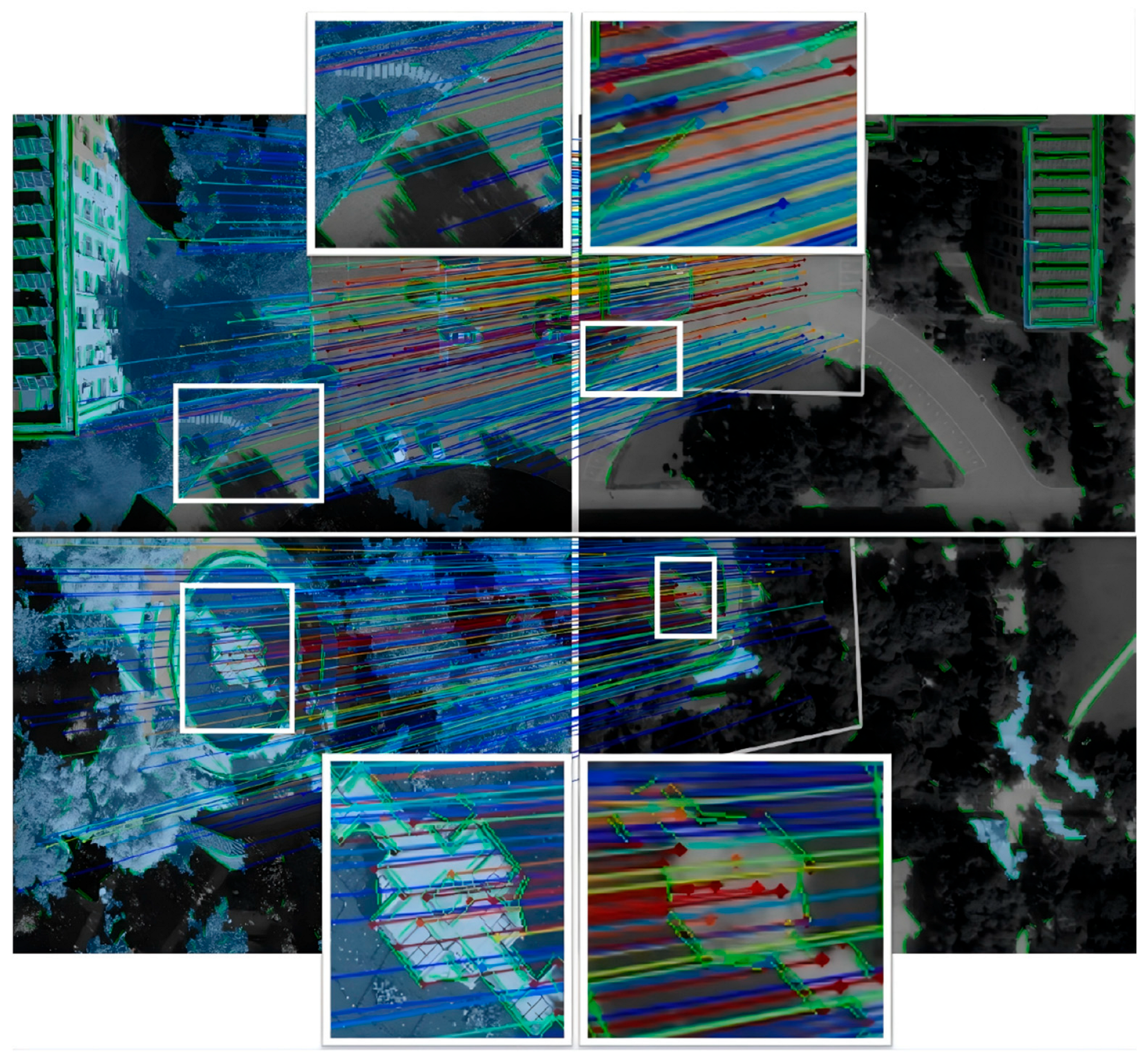
In order to achieve better matching results in weakly textured areas and improve the stability of the matching algorithm, this study improves the original matching algorithm by adding line features and plane features on the basis of the original algorithm. Both are input together with the point features extracted by SuperPoint into the LightGlue matching algorithm to complete image matching.

The Multimodal features + LightGlue image matching algorithm significantly enhances the matching stability of weakly textured regions by introducing a multimodal features collaboration mechanism while maintaining the original lightweight and efficient advantages of the SuperPoint + LightGlue framework. The core of this improvement strategy lies in constructing a complementary fusion system of geometric and semantic features: line features provide long-range geometric constraints by detecting continuous edge structures in the image, while plane features use region segmentation techniques to capture the overall structural information of the scene, forming a hierarchical feature expression with traditional point features.

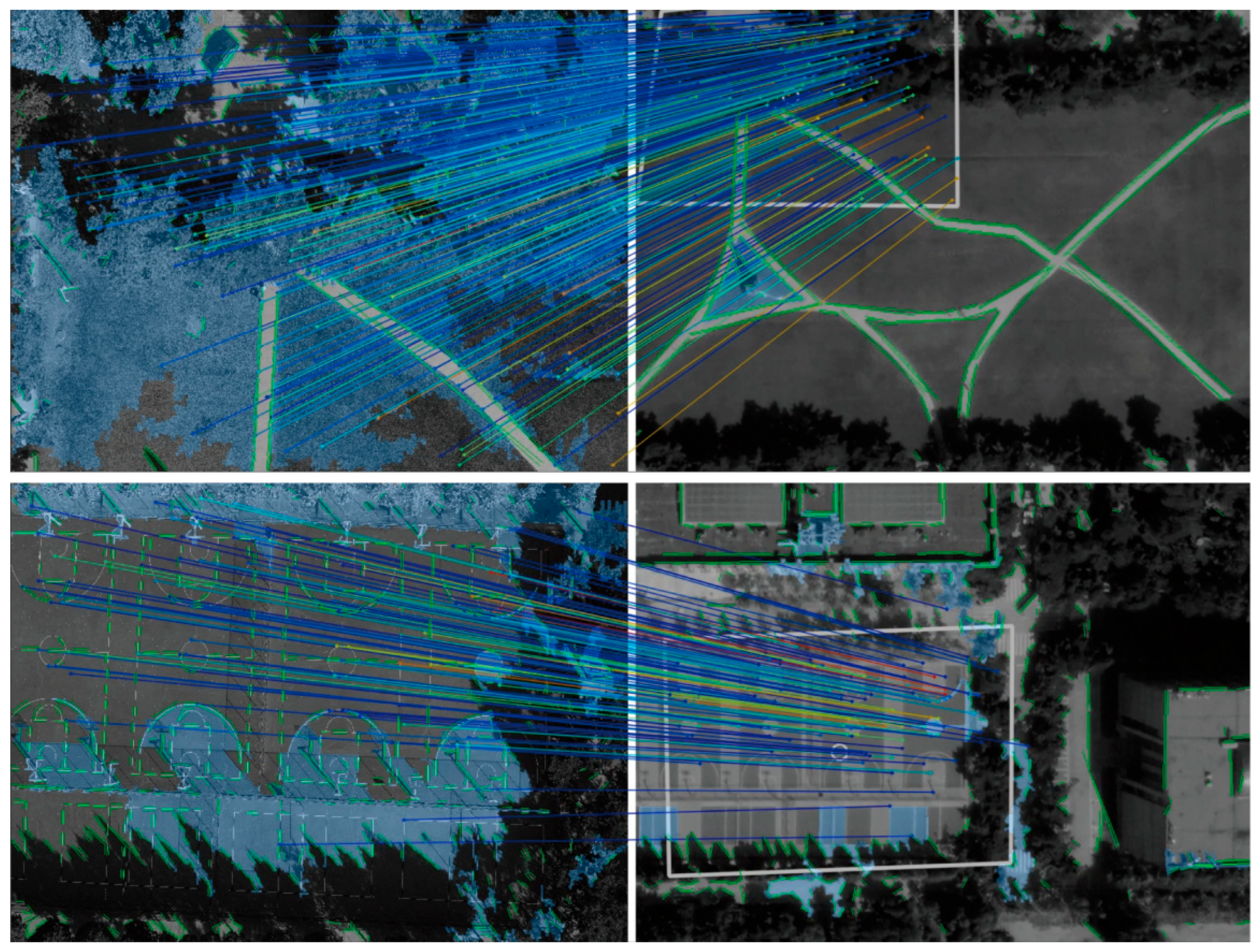
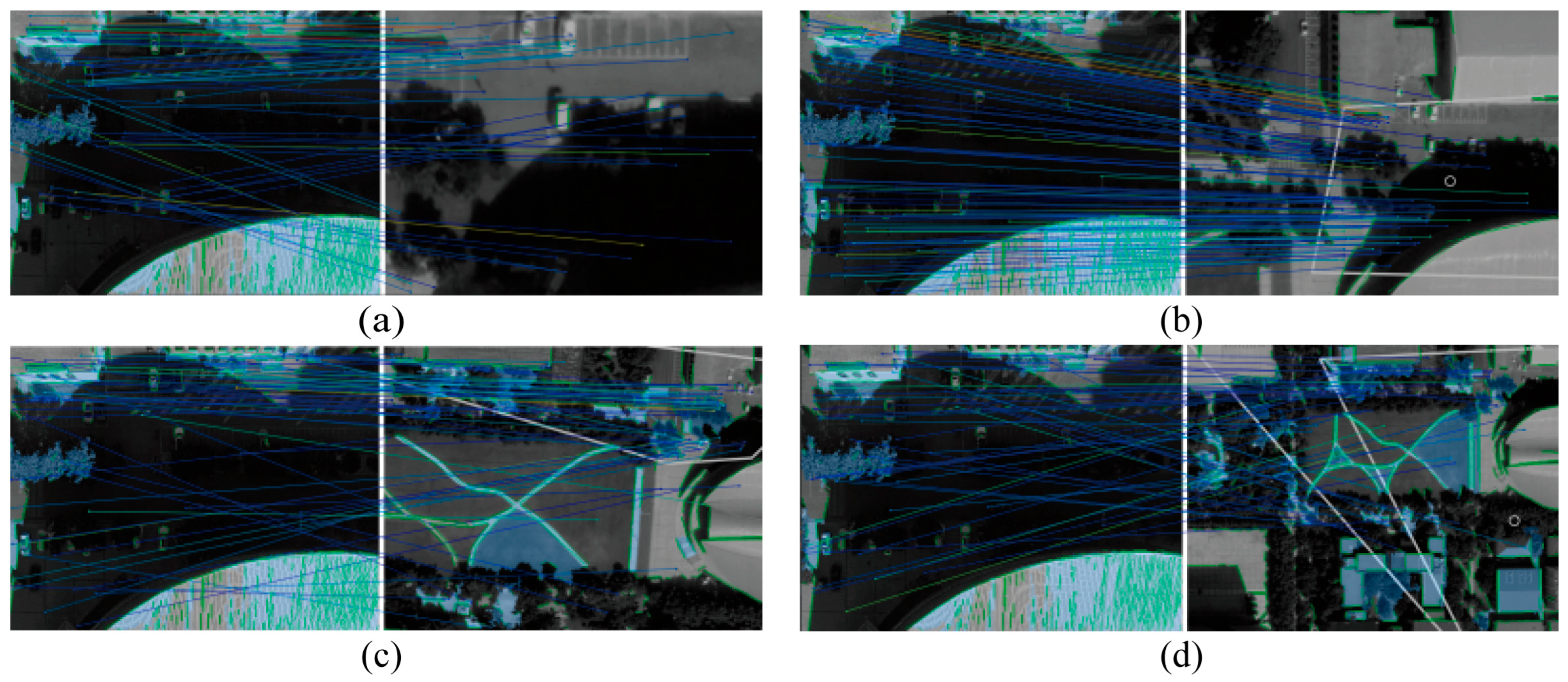
The experimental results shown in Figure 6 indicate that the newly added line plane features contribute a large number of effective matching points in complex scenes with drastic changes in brightness and uneven texture distribution, especially in low-contrast grassland and forest areas commonly seen in drone images, where the density of matching points is significantly increased. Although the average error has slightly increased, the mismatch rate has been reduced and the geometric consistency of the overall matching results has been significantly improved through the verification of regional consistency of plane features and directional constraints of line features.

Regarding computational efficiency, the proposed multimodal framework adheres to a sparse matching paradigm, which is inherently more optimized than dense pixel-level regression methods like LoFTR and RoMa. While the integration of line and plane features introduces a marginal preprocessing overhead, these structural primitives provide robust geometric priors that facilitate faster convergence within the transformer-based LightGlue engine. By leveraging the adaptive “early-exit” mechanism of the matcher, the framework can dynamically terminate computation once confident correspondences are established, often requiring fewer attention layers than single-feature approaches to resolve ambiguities. Consequently, this architectural design ensures that the enhanced matching stability does not come at the cost of prohibitive latency, fulfilling the requirements for near-real-time UAV positioning tasks.

By using feature matching algorithms to match drone images with previous satellite images, real-time localization of drones can be achieved, and the matching results directly affect the accuracy of localization. To rigorously evaluate the performance of the proposed framework, four state-of-the-art image matching algorithms—SuperPoint + SuperGlue [33,34], LoFTR [35], RoMa [36], and SuperPoint + LightGlue [33,37]—were selected as baselines for a comprehensive comparative analysis. Thirty images collected by a drone at an altitude of 80 m in the internal area of the school were selected and matched with satellite images. In addition, experiments were conducted at a flight altitude of 380 m in weakly textured areas (including forests, farmland, etc.) to verify the advantages of our algorithm in weakly textured areas. The matching results are shown in

Table 1. Comparison of matching results of five image matching algorithms.

Algorithm	Position Error (m)
	Within the School	Weak Texture Area
LoFTR	4.18	4.74
RoMa	2.48	8.09
SuperPoint + SuperGlue	0.86	7.21
SuperPoint + LightGlue	0.72	5.89
Multimodal features + LightGlue	0.73	4.62

The positioning error in the table is the average positioning error of the 30 drone images. There are many buildings, roads, etc. in the internal area of the school, with strong texture features. The weakly textured areas mainly include areas with unclear texture features such as forests, farmland, and grasslands.

.

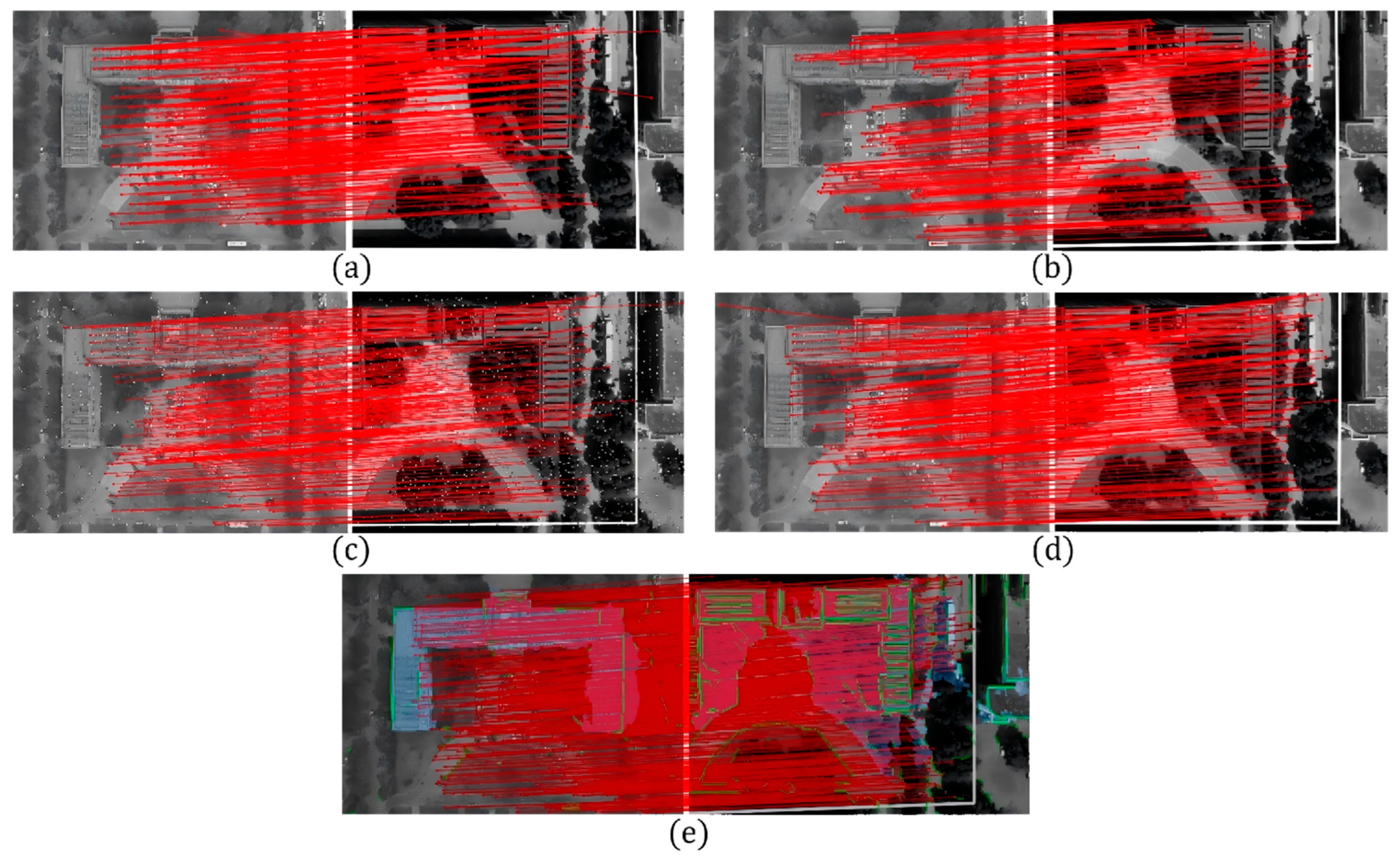
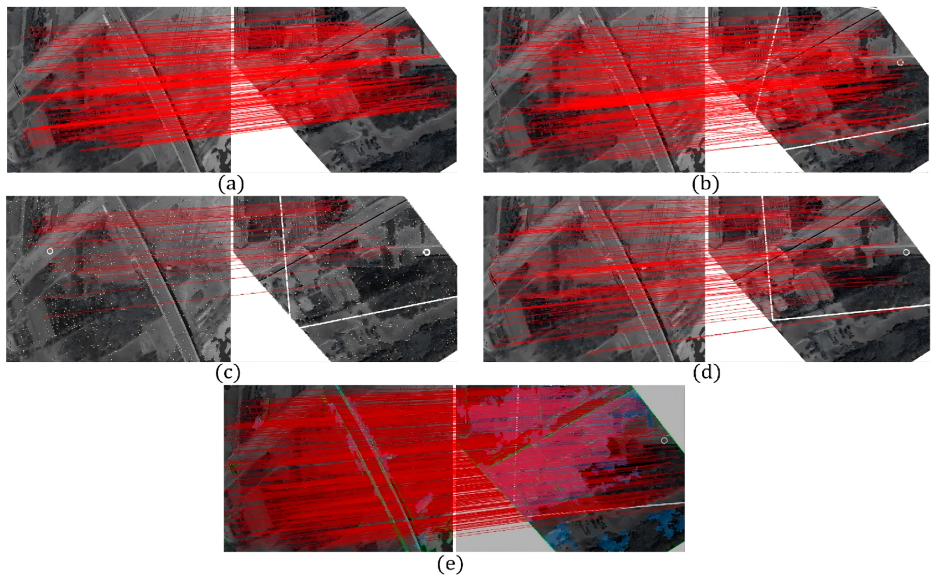
Based on a comprehensive analysis of Table 1 and Figure 7 and Figure 8, it can be seen that in the internal area of the school, due to the presence of numerous buildings, roads, etc., the texture features are rich. The positioning error of the “SuperPoint + SuperGlue” algorithm is 0.86 m, the positioning error of the “SuperPoint + LightGlue” algorithm is 0.72 m, and the positioning error of the “Multimodal features + LightGlue” algorithm proposed in this article is 0.73 m. By comparison, the positioning error of the “LoFTR” algorithm is 4.18 m, and the positioning error of the “RoMa” algorithm is 2.48 m. This indicates that in texture-rich areas, the matching strategy based on the LightGlue algorithm performs better, thanks to the adaptive nature of the LightGlue algorithm. In addition, thanks to the accuracy of SuperPoint feature point extraction, the matching strategy using the SuperPoint algorithm also performs well. The algorithm proposed in this paper, which uses point features, line features, and plane features simultaneously, also has high positioning accuracy.

In the weakly textured area, the positioning error of the “LoFTR” algorithm is 4.74 m, the positioning error of the “RoMa” algorithm is as high as 8.09 m, the positioning error of the “SuperPoint + SuperGlue” algorithm is 7.21 m, the positioning error of the “SuperPoint + LightGlue” algorithm is 5.89 m, and the positioning error of the “Multimodal features + LightGlue” algorithm is 4.62 m.

It can be seen that the positioning errors of various algorithms generally increase in weakly textured areas, but the “Multimodal features + LightGlue” algorithm proposed in this paper has a relatively small positioning error in this area, demonstrating certain advantages. This is because the introduction of multimodal features integrates multiple feature information, making up for the shortcomings of single features in weak texture areas. Combined with the adaptive reasoning ability of the LightGlue algorithm, it can better adapt to the complex situation of weakly textured areas, improving matching accuracy and thereby reducing positioning errors.

Based on the results of two sets of experiments, the “Multimodal features + LightGlue” algorithm demonstrated good performance in different scenarios, maintaining relatively low positioning errors in both texture-rich and weakly textured areas. This verifies the effectiveness and superiority of the algorithm in complex scenarios, providing more reliable technical support for real-time positioning of drones.

4.2. Accuracy Analysis

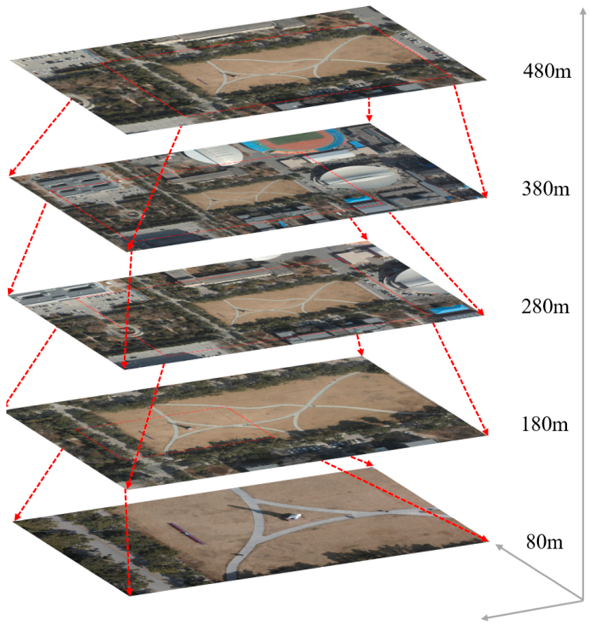
Without using GNSS, the real-time position of the UAV is calculated based on the SuperPoint + LightGlue algorithm. Experiments were carried out at heights of 80 m, 130 m, 180 m, 230 m, 280 m, 330 m, 380 m, 430 m, and 480 m relative to the ground height. The UAV position at the time of image acquisition was calculated. The horizontal distance between the actual position of UAV and the calculated position was used to evaluate the accuracy.

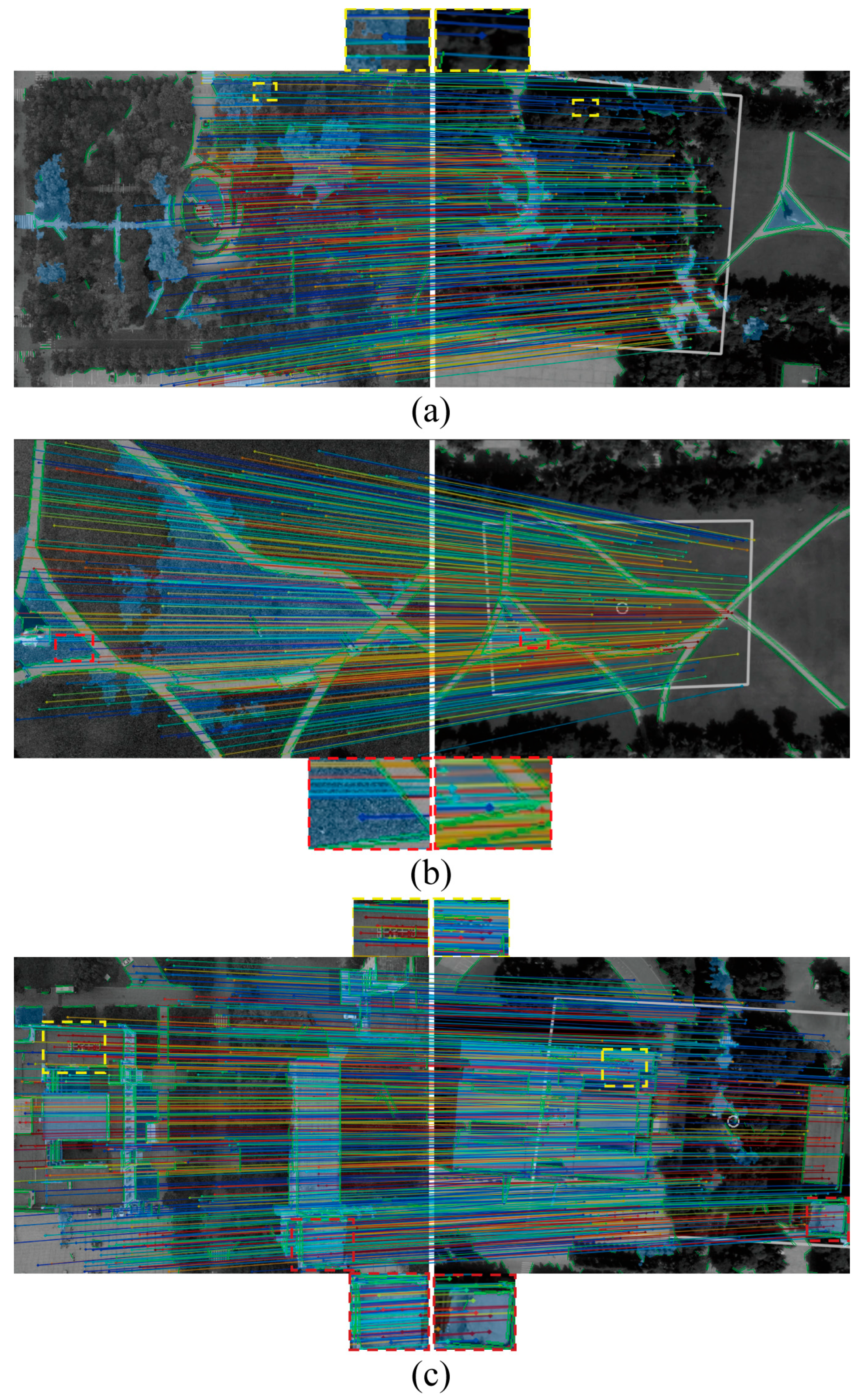
The real-time positioning results of the UAV are shown in Figure 9. It can be seen that there is a significant difference in scale and rotation between the drone images and satellite images, but they also have good matching effects. The SuperPoint + LightGlue algorithm performs well in terms of scale invariance, rotation invariance, and detection robustness.

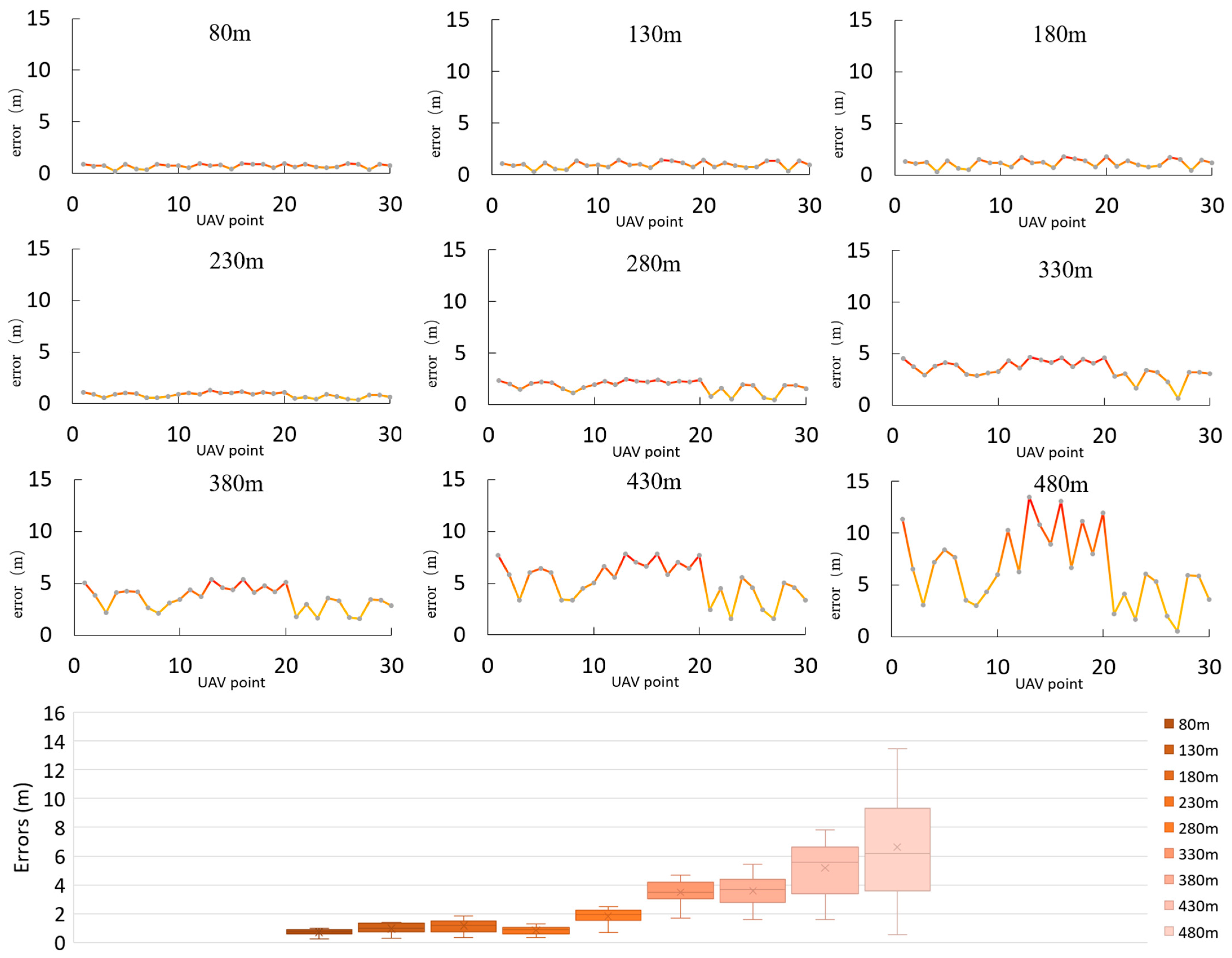
The error of each point of the UAV at different heights is shown in Figure 10 and

Table 2. Statistical analysis of UAV positioning errors.

Height (m)	Mean Error (m)	Max Error (m)	Min Error (m)	Error Less Than 1 m	Error Less Than 5 m	Error Less Than 10 m	Number of Images
80	0.73	1.02	0.22	100%	-	-	30
130	0.95	1.31	0.35	57%	100%	-	30
180	1.21	1.78	0.34	37%	100%	-	30
230	0.88	1.33	0.36	70%	100%	-	30
280	1.83	2.42	0.44	13%	100%	-	30
330	3.32	4.42	0.57	3%	100%	-	30
380	3.43	5.21	1.59	0%	87%	100%	30
430	5.51	6.43	1.58	0%	40%	100%	30
480	6.24	12.54	0.52	3%	33%	77%	30

. When the heights are 80 m, 130 m, 180 m, 230 m, 280 m, 330 m, 380 m, 430 m, and 480 m, the average errors of UAV real-time positioning are 0.73 m, 0.95 m, 1.21 m, 0.88 m, 1.83 m, 3.32 m, 3.43 m, 5.51 m, and 6.24 m, respectively. The highest accuracy is 0.25 m, and the worst is 13.47 m. Additionally, 84% of the points are less than 5 m, 54% are less than 2 m, and 32% are less than 1 m.

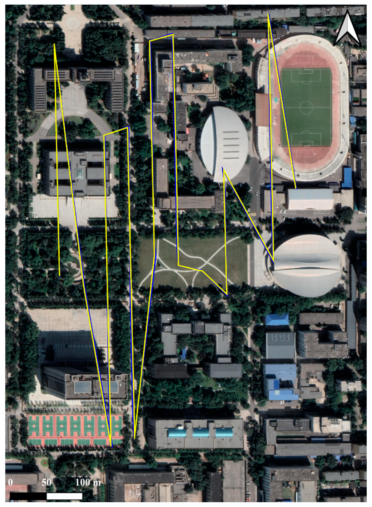
The comparison between the real trajectory and the calculated trajectory of the drone is shown in Figure 11. This trajectory is the trajectory of the drone flying at an altitude of 80 m. It can be seen from the figure that the calculated trajectory is highly consistent with the real trajectory.

5. Discussion

5.1. Effect of the Type of Ground Objects and the Change in Season on Matching Results

In Figure 10, it can be observed that at the same flight altitude, the accuracy fluctuates significantly and is relatively low for some points. To address this, we conducted an analysis from two aspects: the type of ground objects and the change in season.

Figure 12 demonstrates the impact of differences in ground object type on positioning accuracy, where Figure 12a,b indicate that the matching result between the drone and satellite images is located in areas with relatively high tree and grassland coverage. From the local magnification of the matching points, it can be seen that there is a deviation in the matching points, which undoubtedly affects the accuracy of positioning. The drone flight altitude at this point is 180 m, and the positioning errors of drones over grasslands and forests are 1.81 m and 1.78 m, respectively, which belongs to the point with a large error at a flight altitude of 180 m. When the drone is above the building, as shown in Figure 12c, the positioning error is 0.32 m. This is mainly because images with more buildings have more distinct texture features and more selectable feature points, resulting in better matching effects and higher accuracy.

Another reason for the large error is that the drone images and satellite images were taken at different time periods, and vegetation and other ground objects change greatly with time and season, where these differences can be observed in Figure 13, directly affecting the image matching effect and leading to the low positioning accuracy of UAVs. To verify this result, we selected drone images from winter and summer and satellite images from summer for matching.

Thirty images taken at a height of 80 m were selected for accuracy comparison. The positioning error of drone images taken in winter is 1.34 m, and the positioning error of drone images taken in summer is 0.73 m. The experiment also proved that the positioning accuracy will be affected when the UAV flies over a large area of trees and grass. As shown in Figure 14, the Google image was collected on 31 March 2024, and the drone image was collected on 22 March 2025. In agricultural areas, not only are there fewer texture features, but human activities such as spring sowing and autumn harvesting greatly change their texture features.

5.2. Effect of Height and the Scale of Satellite Imagery on Matching Results

In order to verify the universality of the matching algorithm in the low airspace of UAVs and meet the application needs of UAVs in a complex environment, UAV positioning experiments were carried out at 80 m, 130 m, 180 m, 230 m, 280 m, 330 m, 380 m, 430 m, and 480 m away from the ground. The positioning results are shown in

Table 3. Image parameters of UAV flying at different altitudes.

Height (m)	Spatial Resolution (cm)	Coverage Area (m2)	Mean Error (m)
80	0.94	3952	0.73
130	1.63	11,883	0.95
180	2.26	22,845	1.21
230	2.89	37,357	0.88
280	3.52	55,420	1.83
330	4.14	76,662	3.32
380	4.77	101,769	3.43
430	5.40	130,427	5.51
480	6.00	161,021	6.24

. Overall, as the height increases, the spatial resolution of drone images decreases and the positioning accuracy gradually decreases.

As the UAV rises in height, the spatial resolution of the UAV image is also lower. As shown in Table 3, when the flight altitude is 80 m, the spatial resolution of the image is 0.94 cm, and when the flight altitude is 480 m, the spatial resolution of the image is 6 cm. The spatial resolution of UAV images taken 80 m from the ground is more than 6 times that of UAV images taken 480 m from the ground. In addition, since the image taken by the UAV is orthophoto, the plane coordinate of the central position of the UAV image is determined to be the real-time coordinate of the UAV. However, factors such as flight attitude fluctuations, wind-induced jitter, and gimbal angular bias introduce an offset angle ($\theta$), causing the calculated coordinates to deviate from the true position. This deviation causes the calculated image center to shift away from the true horizontal position of the UAV, serving as the primary source of positioning error. Quantitatively, this geometric displacement ($E$) is governed by the relationship $E=H\cdot \mathit{tan}(\theta )$. Consequently, the positioning error exhibits a progressive increase as a function of altitude, as the same angular perturbation is amplified over greater vertical distances. To further quantify this sensitivity, the theoretical horizontal errors associated with angular deviations of $1^{\circ }$, ${0.1}^{\circ }$, and ${0.01}^{\circ }$ across the experimental altitudes are detailed in

Table 4. Theoretical horizontal positioning errors induced by different angular deviations across various flight altitudes.

Flight Altitude (m)	$1^{\circ }$ Error (m)	${0.1}^{\circ }$ Error (m)	${0.01}^{\circ }$ Error (m)
80	1.40	0.14	0.014
130	2.27	0.23	0.023
180	3.14	0.31	0.031
230	4.01	0.40	0.040
280	4.89	0.49	0.049
330	5.76	0.58	0.058
380	6.63	0.66	0.066
430	7.51	0.75	0.075
480	8.38	0.84	0.084

.

It is known that for a UAV shooting at different heights, the field of view of UAV images is different, as shown in Figure 15. The coverage area of UAV images taken 480 m above the ground is about 161,021 ${\mathrm{m}}^2$ and the coverage area of UAV images taken 80 m above the ground is about 3952 ${\mathrm{m}}^2$. The coverage area of the UAV image taken at a height of 480 m from the ground is about 40 times that of a UAV image taken 80 m from the ground. The larger the field of vision, the more features in the image, which means that more feature points can be detected and more image pairs can be matched. This is also the reason why the positioning error becomes lower when the drone flies at an altitude of 230 m.

In addition, the scale of satellite imagery also affects the accuracy of drone positioning. Given that the ground sampling distance (GSD) of UAV imagery varies with flight altitude, we introduced the side-length ratio ($R$) to quantitatively define the satellite image scale $R=L_{sat}/L_{uav}$, where $L_{sat}$ and $L_{uav}$ represent the actual ground side lengths covered by the satellite reference image and the UAV real-time image, respectively. We believe this dimensionless ratio provides a more scale-adaptive metric for multi-altitude operations, ensuring a consistent geometric relationship regardless of variations in spatial resolution.

Taking a set of images collected by a drone at 180 m as an example, the impact of satellite image scale is verified by comparing the UAV images with satellite imagery at four different side-length ratios of approximately 1, 1.5, 4, and 8 (corresponding to scale levels 1 to 4 in Figure 16). Figure 16 shows the matching results across these varying field-of-view ranges. The experimental observations indicate that the optimal matching effect is achieved at scale level 2, where the ratio is approximately 1.5.

This performance gain may stem from the relative scale of identical features between the UAV and satellite images at this specific ratio being inherently more suitable for the matching algorithm’s operational requirements. Additionally, the 1.5 ratio provides a contextual buffer; compared to the 1.0 ratio, it likely offers the necessary surrounding structural information for feature descriptors. In our test, this is accompanied by an 18% increase in the number of successfully matched feature pairs. However, when the ratio increases to 4 or 8, the successful matching rate tends to decrease. This trend may be attributed to the expanded search area introducing excessive irrelevant textures or repetitive patterns. Furthermore, it is also possible that the increased ambiguity or blurring of feature structures within a broader search space leads to a decrease in the successful matching rate.

6. Conclusions

In response to the problem of GNSS signal interference or GNSS signal loss in weak GNSS environments, we propose the Multimodal features + LightGlue image matching algorithm, which matches the real-time collected images of a drone with previous satellite images and then calculates the real-time position of the drone. To verify the advancement of the proposed algorithm, it is compared with four advanced image matching methods, that is LoFTR, RoMa, SuperPoint + SuperGlue, and SuperPoint + LightGlue. The results indicate that the Multimodal features + LightGlue image matching algorithm proposed in this paper is more suitable for matching drone images with satellite images and has better matching accuracy in areas with strong and weak texture features. The experimental results show that the positioning accuracy gradually decreases with increasing altitude from 80 m to 480 m, while the average error of real-time positioning of drones increases from 0.73 m to 6.24 m. From the analysis of the experimental results, it can be seen that the positioning accuracy of drones is mainly affected by the type of ground objects, seasonal changes, the altitude of drone flight, and the scale of satellite images. Overall, this study provides both a theoretical basis and practical solutions for drone localization in complex scenarios, holding significant potential for engineering applications.