A Bias Correction Scheme for FY-3E/HIRAS-II Data Assimilation Based on EXtreme Gradient Boosting

Highlights

What are the main findings?

• The XGBoost bias correction can effectively eliminate the linear and nonlinear biases.
• The bias correction based on linear regression may not be applicable to HIRAS-II.

What are the implications of the main findings?

• The mean and standard deviation of O-B in all channels are the smallest after XGBoost bias correction and the effective observations through quality control are the largest.
• The XGBoost bias correction can improve the accuracy of temperature analysis fields.

Abstract

More and more spaceborne infrared hyperspectral atmospheric observations are assimilated into data assimilation systems. The key to bias correction (BC) of these instruments depends on selecting predictors. However, it is difficult to find a set of predictors that are highly correlated with the O-B biases in all FY-3E/HIRAS-II channels, due to its multi-channel characteristics. A machine learning model XGBoost (EXtreme Gradient Boosting) BC scheme for FY-3E/HIRAS-II is established in this article. The selected predictors include model skin temperature, model total column water vapor, 1000–300 hPa thickness, 200–50 hPa thickness, scan position, observed brightness temperature (BT) and simulated BT. The method is also compared with the operational static BC and the variational BC, to validate its effect. The two-week data assimilation experiments show that the XGBoost BC is the most effective among the three BC schemes. The mean and standard deviation of O-B in all channels are the smallest after BC, and the effective observations through quality control are the largest, followed by the static BC. The static BC and variational BC are performed based on linear regression, which may lead to a small loss of valid observations in some channels that are weakly correlated with the predictor, whereas machine learning algorithms can search for the nonlinear correlation between biases and predictors. Compared with ERA5, both temperature- and humidity-analysis fields based on XGBoost BC are closest to ERA5 at all levels, and the root mean square errors do not change much over time.

1. Introduction

The purpose of data assimilation (DA) is to provide optimal initial conditions for numerical weather prediction (NWP) [1]. Due to the advantages of wide coverage and high spatial–temporal resolution, satellite observations have become an extremely important data source for DA. Among them, the spaceborne infrared hyperspectral atmospheric sounders can obtain a large amount of atmospheric radiance data with high vertical resolution. These observations have been widely used in NWP and have had a positive impact [2]. Fengyun-3E (FY-3E) is the world’s only dawn–dusk polar-orbiting meteorological satellite, and its launch effectively supplements the gap in satellite observations in the 6 h assimilation window [3]. HIRAS-II (Hyperspectral Infrared Atmospheric Sounder-II) is the world’s only infrared atmospheric sounder operating in dawn–dusk orbit, whose radiance data are accurately assimilated and can potentially improve the accuracy of NWP.

The difference between the observed value O and the simulated value B (simulated by the observation operator) is called bias (O-B). The biases in observations are highly susceptible to damaging the DA analysis, and thus affect the forecast accuracy of NWP [4,5]. Biases in assimilating the satellite radiance observations are particularly noteworthy because satellite observations now comprise the vast majority of all existing atmospheric observations [6]. There are inevitable systematic biases between observations and simulations, which can corrupt NWP forecasts in a short period [7]. The simulated errors may originate from the accuracy of the radiative transfer model or the NWP forecast data (e.g., the temperature and humidity profiles, surface temperature, wind speed as input to the fast radiative transfer model). Furthermore, the use of a fixed surface emissivity value (over land) for IR instruments will introduce significant additional error [8]. The observed errors may arise from residual biases in the satellite data calibration, data preprocessing steps, etc. These errors combine to form the systematic biases between the satellite observations and the model simulations. The accuracy of NWP will be greatly affected if the systematic biases are not corrected [4,9]. Before applying satellite observations to DA systems, the systematic biases must be reasonably estimated and corrected to meet the assumption that both observation and background errors are unbiased, as required by the variational assimilation method [10].

At present, the bias correction (BC) of satellite DA is based on the linear relationship between biases and predictors. The variational BC updates the BC coefficients simultaneously during iterative minimization by adding predictor coefficients to the control variables. Although the coefficients change with time and weather systems, it is still essentially fitting the linear relationship between predictors and biases through a linear regression [9,11]. Therefore, the key to BC depends on selecting highly linearly correlated predictors. Eyre used the MSU (Microwave Sounding Unit) radiance as predictors to implement BC for TOVS (The TIROST Operational Vertical Sounder) [7]. Harris and Kelly established a two-step BC method (scan-angle BC and airmass BC), using 1000–300 hPa thickness, 200–50 hPa thickness, model skin temperature and model total column water vapor as predictors for the airmass BC after scan-angle BC [12]. The above BC schemes are static offline operations, and the BC coefficients are fitted by multiple linear regression based on the long-term statistical biases and predictors without considering the evolution of biases with time, so the assimilation systems have to be interrupted and restarted on many occasions, for manual retuning of the bias corrections [13]. Therefore, it is of great significance to consider a dynamic BC method that can periodically update the BC coefficients. Among them, an adaptive offline BC (also known as “cycling” BC) is commonly employed in the early operational data assimilation. This approach periodically re-estimates BC coefficients using a sliding time window, allowing them to be updated cyclically and thus exhibit time-varying characteristics [4]. Subsequently, many scholars developed variational BC schemes that dynamically update BC coefficients by adding coefficients in the control variable. The fundamental difference between the two adaptive BC methods is that the former updates the coefficients prior to the analysis (assuming the NWP model fields to be correct), while the latter updates them within the analysis (assuming that the observation bias does not change abruptly). Derber and Wu used a function reflecting the vertical variation of atmospheric temperature as a predictor when assimilating MSU radiance data in the NECP (the National Centers for Environmental Prediction)–GSI (Gridpoint Statistical Interpolation) operational system [14]. The predictor has been used in the NECP-GSI operational system until now. Dee established the variational BC module in the ECMWF (European Centre for Medium-Range Weather Forecasts) DA system and selected different predictors for different satellite instruments [15]. Zhu et al. modified the variational BC scheme in NCEP-GSI and improved the scan-angle predictor to implement the variational BC in one step [16]. Li et al. evaluated the applicability of airmass predictors in the GSI operational DA system for S-NPP/CrIS, and proposed a BC scheme based on the CrIS periodic O-B bias characteristics [2]. Otkin et al. established a BC scheme with a Taylor series polynomial expansion of the OMB biases, and successfully eliminated linear and nonlinear biases in the all-sky assimilation of SEVIRI (Spinning Enhanced Visible and Infrared Imager) radiance data. The study also demonstrated the feasibility of using observed BT as a predictor [17]. Zhang et al. used a BC scheme based on Random Forest to correct the biases of FY-4A/AGRI (Advanced Geosynchronous Radiation Imager) infrared radiance. Their results showed that the observed BT and simulated BT had a certain effect on removing nonlinear biases [18]. Currently, there are fewer studies on the BC for FY-3E/HIRAS-II. Liu et al. assimilated FY-3E/HIRAS-II radiance observations based on the CMA (China Meteorological Administration)-GFS (Global Forecast System), and 1000–300 hPa thickness, 200–50 hPa thickness and 50–10 hPa thickness are used as predictors in the BC [19]. Chen and Guan used four predictors (background field temperature, total water vapor, 1000–300 hPa thickness and 200–50 hPa thickness) as the optimal combination for FY-3E/HIRAS-II, after evaluating the importance of predictors [20]. However, it is difficult to find a set of predictors that are highly correlated with all assimilated channels, due to the multi-channel characteristic of FY-3E/HIRAS-II. It may lead to residual nonlinear biases after BC if the predictors are weakly correlated with some assimilated channels.

The tree algorithms have been widely used in regression problems. One of the excellent properties of regression tree is the flexibility in fitting, because it can accurately capture the nonlinear characteristics of data [21]. Zhang et al. proposed a BC method based on Random Forest, effectively eliminating the linear and nonlinear biases in the all-sky assimilation of FY-4A/AGRI infrared channels 9 and 10 [18]. It verified the effectiveness of the regression tree in nonlinear BC. Due to the multi-channel (thousands of channels) characteristic of FY-3E/HIRAS-II, the number of FY-3E/HIRAS-II observations in one assimilation process is several hundred times that of FY-4A/AGRI. Therefore, a machine learning model with faster training and testing speeds is needed for the FY-3E/HIRAS-II BC. XGBoost (eXtreme Gradient Boosting) is an ensemble learning algorithm based on gradient boosting, which has fast speed and generalization ability when dealing with large-scale and complex datasets [22].

Therefore, this study selects a combination of predictors to establish a new FY-3E/HIRAS-II BC scheme based on XGBoost. It is also compared with the commonly used static BC scheme and the variational BC scheme in the WRFDA (Weather Research and Forecasting Data Assimilation) system. Finally, the effect of the different BC schemes is objectively evaluated through two-week FY-3E/HIRAS-II DA experiments.

2. Data and Model

2.1. HIRAS-II Data

HIRAS-II is an infrared atmospheric sounder operating in dawn–dusk orbit. It observes the atmosphere through a cross-track scan mode, and each scan line includes 28 contiguous ground fields of regard (FORs). Each FOR is composed of a 3 × 3 field-of-view (FOV, the spatial resolution at nadir is 14 km) array. HIRAS-II provides continuous infrared radiance in the band cover 3.92~15.38 μm (650~2550 cm⁻¹), with a channel spacing of 0.625 cm⁻¹. The HIRAS-II data are obtained from Fengyun Satellite Data http://data.nsmc.org.cn/DataPortal/cn/home/index.html (accessed on 24 February 2026).

ERA5 (ECMWF Reanalysis version 5) is the fifth-generation ECMWF reanalysis for the global climate and weather for the past 8 decades. ERA5 is a regular grid dataset with a horizontal spatial resolution of 0.25° × 0.25° and 37 vertical levels from 1000 hPa to 1 hPa. The data contains various atmospheric and surface parameters. The ERA5 data can be obtained from the Copernicus Climate Change Service: https://cds.climate.copernicus.eu (accessed on 24 February 2026).

2.2. HIRAS-II Clear-Sky Assimilation Module in WRFDA

In this study, the WRFDA v4.5.1 is used to evaluate the effectiveness of different BC methods on the FY-3E/HIRAS-II DA experiments. WRFDA is a DA system developed by the National Center for Atmospheric Research (NCAR), and can assimilate various observations. The fundamental principle of the WRFDA three-dimensional variational assimilation system is to minimize the cost function $J\left(x\right)$ [23]:

$$J\left(x\right)={\displaystyle \frac{1}{2}}{\left(x-x_b\right)}^T{B}^{-1}\left(x-x_b\right)+{\displaystyle \frac{1}{2}}{\left(y-H\left(x\right)\right)}^T{\left[O+F\right]}^{-1}\left(y-H\left(x\right)\right)$$

(1)

where $x_b$ is the background field, $y$ is the observation field, $x$ is the atmospheric state vector, $B$ is the background error covariance, $\left[O+F\right]$ is the observation and direct mode error covariance, and $H$ is the observation operator. (The fast radiative transfer mode RTTOV v12.3 is used as the observation operator in this article, in which the emissivity of land surface is set to the fixed value 0.98. The terrain height used in simulating the HIRAS-II BT by RTTOV is from HIRAS-II level 1 data.)

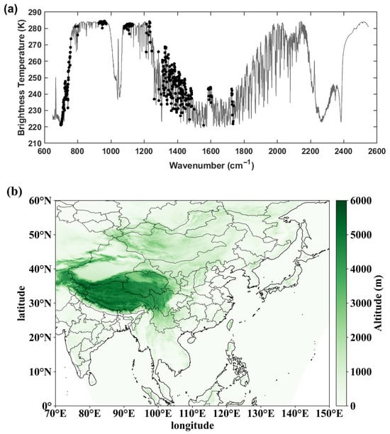
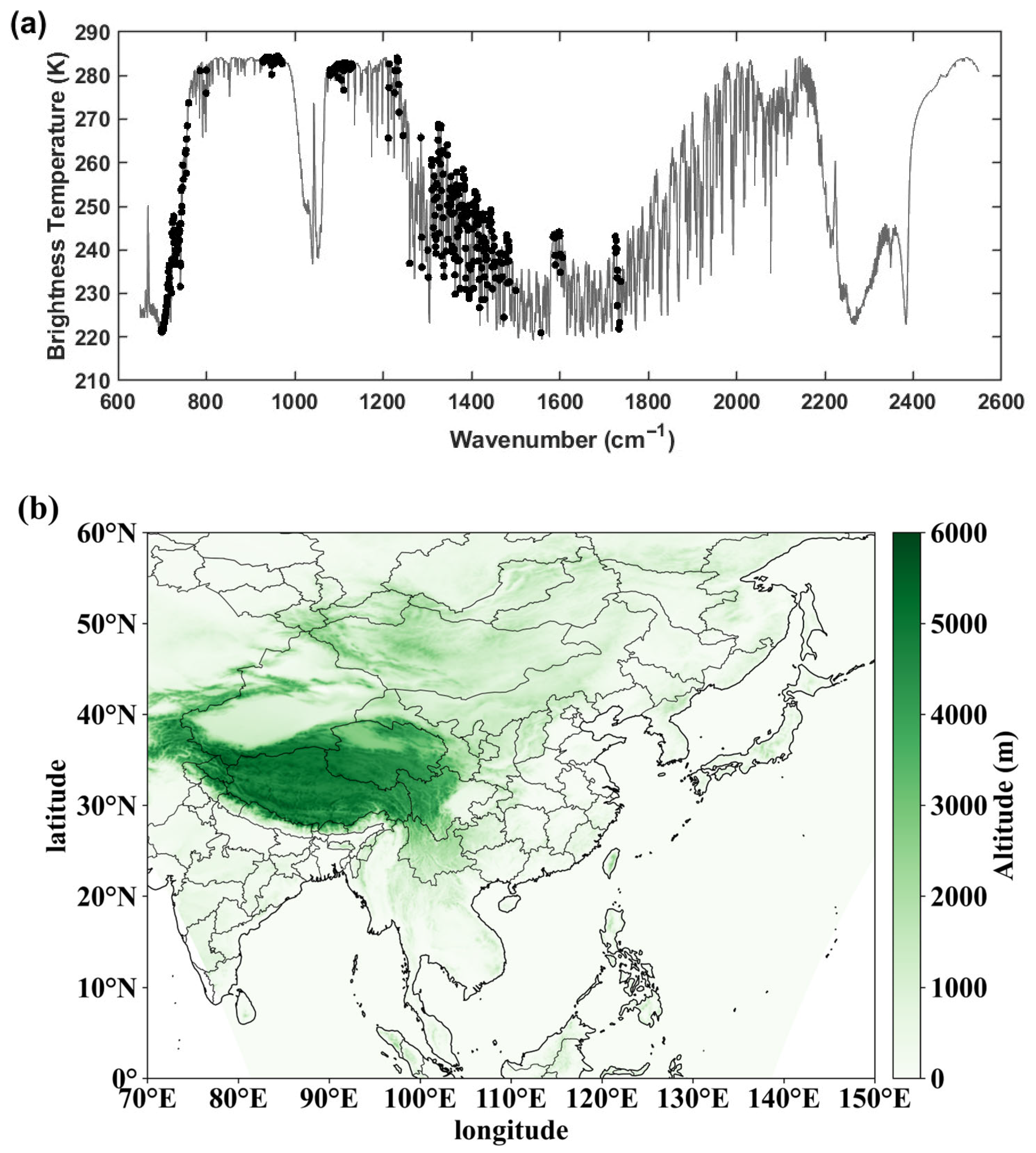
The FY-3E/HIRAS-II DA has not been implemented in WRFDA. A new FY-3E/HIRAS-II DA module is established in WRFDA by adding quality control (QC) and reading interfaces. Based on the 537 assimilated channels recommended in the FY-3E/HIRAS-II L1C level products users’ guide provided by the Fengyun Satellite Remote Sensing Data Service Network (https://img.nsmc.org.cn/PORTAL/NSMC/DATASERVICE/OperatingGuide/FY3E/FY-3E_Product_Instruction_HIRAS-II_DAS.pdf (accessed on 24 February 2026)), the shortwave channels with poor quality and which are susceptible to non-local thermal equilibrium (NLTE) effects are excluded. The O₃ absorption channels are also excluded (in the absence of real O₃ profiles, there are significant positive biases in bright temperatures simulated using default values [24]). A total of 401 HIRAS-II channels are selected to assimilate (the wavenumbers of the assimilated channels are provided in the Supplementary Materials). Figure 1 shows the simulated BT of all HIRAS-II channels calculated by RTTOV using a US76 standard atmosphere profile. The black dots in Figure 1 represent the assimilated HIRAS-II channels. The weight functions of the 401 selected channels show that the selected channels include longwave CO₂ channels, water vapor channels on the left wing and some window channels and cover almost uniformly at all heights. For data thinning, only the observation from the central fifth FOV within each FOR (including 3 $\times$ 3 FOVs) is retained. The detailed QC steps are as follows: (a) reject observations affected by clouds using the MR (Minimum Residual) cloud detection method [25] (the HIRAS-II channels used in the method are listed in the Supplementary Materials); (b) reject observations in channels where the peak height of weight function is lower than the terrain; (c) if the observed BT in any channel exceeds a threshold value (150–350 K), all channel observations in the FOV are discarded. If the absolute value of O-B in any channel is greater than three times its standard deviation, the channel is discarded; and (d) the observations from coastal pixels (land–sea boundaries) are discarded. The main research region of this article is the Chinese region, and the specific area (approximately between 0°N~60°N and 70°E~150°E) is shown in Figure 1b. The green shading represents the terrain heights. The region can acquire the largest number of FY-3E/HIRAS-II observations within the 6 h assimilation time window (almost full coverage at assimilation times at 0000 UTC and 1200 UTC).

Figure 1. (a) Simulated HIRAS-II BT (gray line) by the RTTOV using the US76 standard atmospheric profile, and the assimilated 401 HIRAS-II channels (black dots). (b) The research domain; green shading is altitude.

3. Bias Estimation and BC Schemes

3.1. Bias Estimation

In the satellite DA system, observation (O) error and background (B) error are assumed to be unbiased. If the unbiased assumption does not hold, the biases ${\mu }_o=\overline{O-T}$ and ${\mu }_b=\overline{B-T}$ of the observation error and background error must be subtracted from the observed BT and simulated BT, respectively, where $T$ denotes the true value. The O-B in the cost function is replaced with the following equation, due to the existence of observation error and background error [9]:

$$\left(O-{\mu }_o\right)-\left(B-{\mu }_b\right)=O-B-\left({\mu }_o-{\mu }_b\right)=O-B-{\mu }_{O-B}$$

(2)

where observation error is ${\mu }_o=\overline{O-T}$, background error is ${\mu }_b=\overline{B-T}$, $T$ is the true value, and ${\mu }_{O-B}$ is the bias of observed and simulated BT. The above expression provides the theoretical basis for BC and bias estimation. Since

$$\overline{O-B}-{\mu }_{O-B}=\left(\overline{O-T}-{\mu }_o\right)-\left(\overline{B-T}-{\mu }_b\right)=0$$

(3)

then

$${\mu }_{O-B}=\overline{O-B}$$

(4)

Therefore, the ${\mu }_{O-B}$ can be estimated without knowing the $T$ based on the O-B samples, without the need to estimate ${\mu }_o$ and ${\mu }_b$ separately.

3.2. BC Schemes

3.2.1. Static BC Scheme

This study establishes a static BC scheme based on the Harris and Kelly method [13]. The scheme includes two steps: the scan-angle BC and the airmass BC.

HIRAS-II is a cross-track scanning instrument; the FOV is prone to deformation when the satellite instrument scans both sides, leading to unavoidable biases relative to the nadir FOV [26]. The optical path length is longer as the scan angle increases, which leads to scan-angle biases. In addition, although the fast radiative transfer models can simulate the BT at different scan angles now, the atmospheric inhomogeneity increases with the increase in scan angle. If the model cannot fully simulate atmospheric inhomogeneity, it may also lead to biases in the simulated BT, which depends on the scan angle [27]. For each channel, the mean difference of each scan position relative to the nadir FOV is calculated:

$$S\left(\theta \right)=\overline{R}\left(\theta \right)-\overline{R}\left(\theta =0\right)$$

(5)

where $\overline{R}$ is the mean BT at different scan positions, $\theta$ is the scan position, and $S\left(\theta \right)$ is the scan-angle BC coefficient, applying the following equation can obtain the bias corrected after the scan-angle BC:

$$R^{\prime }\left(\theta \right)=R\left(\theta \right)-S\left(\theta \right)$$

(6)

The four airmass predictors (namely 1000–300 hPa thickness, 200–50 hPa thickness, model surface skin temperature and model total column water vapor) are the default set used for all instruments in WRFDA [28]. The multiple linear regression is established to calculate the airmass bias for each channel $j$, based on the association of the predictors $x_i(\mathrm{i}=\mathrm{1,2},\dots ,4)$ with the airmass bias:

$$r_j=\sum _{i=1}^n{a}_{ji}{x}_i+c_j$$

(7)

where $a_{ji}$ and $c_j$ are calculated by the least-squares fitting and $r_j$ is the airmass bias in each channel, applying the following equation can accomplish airmass BC:

$$R_j^{″}=R_j^{\prime }-r_j$$

(8)

where $R_j^{\prime }$ is the bias after scan-angle BC in each channel, and $R_j^{″}$ is the bias after airmass BC.

3.2.2. Variational BC Scheme

The static BC scheme does not consider the variation in BC coefficients over time, whereas the variational BC scheme is often adopted in practical DA systems. The BC coefficients of predictors are added to the cost function $J\left(x\right)$ in Equation (1), and adaptively updated in the process of minimizing the cost function:

$$\begin{array}{c}J\left(x\right)={\displaystyle \frac{1}{2}}{\left(x-x_b\right)}^T{B}^{-1}\left(x-x_b\right)+{\displaystyle \frac{1}{2}}{\left(y-H\left(x\right)\right)}^T{\left[O+F\right]}^{-1}\left(y-H\left(x\right)\right)\\ +{\displaystyle \frac{1}{2}}{\left(\beta -{\beta }_b\right)}^T{B}_{\beta }^{-1}\left(\beta -{\beta }_b\right)\end{array}$$

(9)

where $\beta$ is the BC coefficients, ${\beta }_b$ is the priori estimate of $\beta$, and $B_{\beta }$ is the error covariance of $\beta$.

The Static BC corrects scan-dependent biases using a pre-computed, position-specific offset $S\left(\theta \right)$, while the VarBC models it via a low-order polynomial fit with coefficients solved within the assimilation. The scan-dependent predictors for VarBC include scan position, the second order of scan position and the third order of scan position. These coefficients will be updated with other predictor coefficients during the WRFDA minimization process. Therefore, the seven predictors used in WRFDA variational BC are 1000–300 hPa thickness, 200–50 hPa thickness, model surface skin temperature, model total column water vapor, scan position, the second order of scan position and the third order of scan position. The airmass bias in each channel is the sum of the products of all predictors and BC coefficients:

$$r_j^{\prime }={\sum }_{i=1}^n{\beta }_{i,j}{\times P}_{n,i,j}$$

(10)

where $r_j^{\prime }$ is the airmass bias in each channel, $\beta$ is BC coefficients, and $P$ is the predictors.

3.2.3. BC Scheme Based on the XGBoost

Based on the research of Qtkin et al. [17] and Zhang et al. [18], the scan position, observed BT and simulated BT are added as predictors to the combination of predictors used in the static BC scheme proposed by Chen and Guan [20]. The optional predictors for FY-3E/HIRAS-II are model skin temperature, model total column water vapor, 1000–300 hPa thickness, 200–50 hPa thickness, scan position, observed BT, and simulated BT.

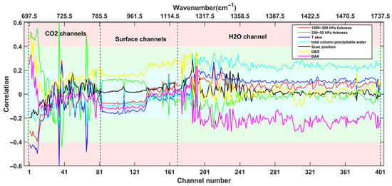
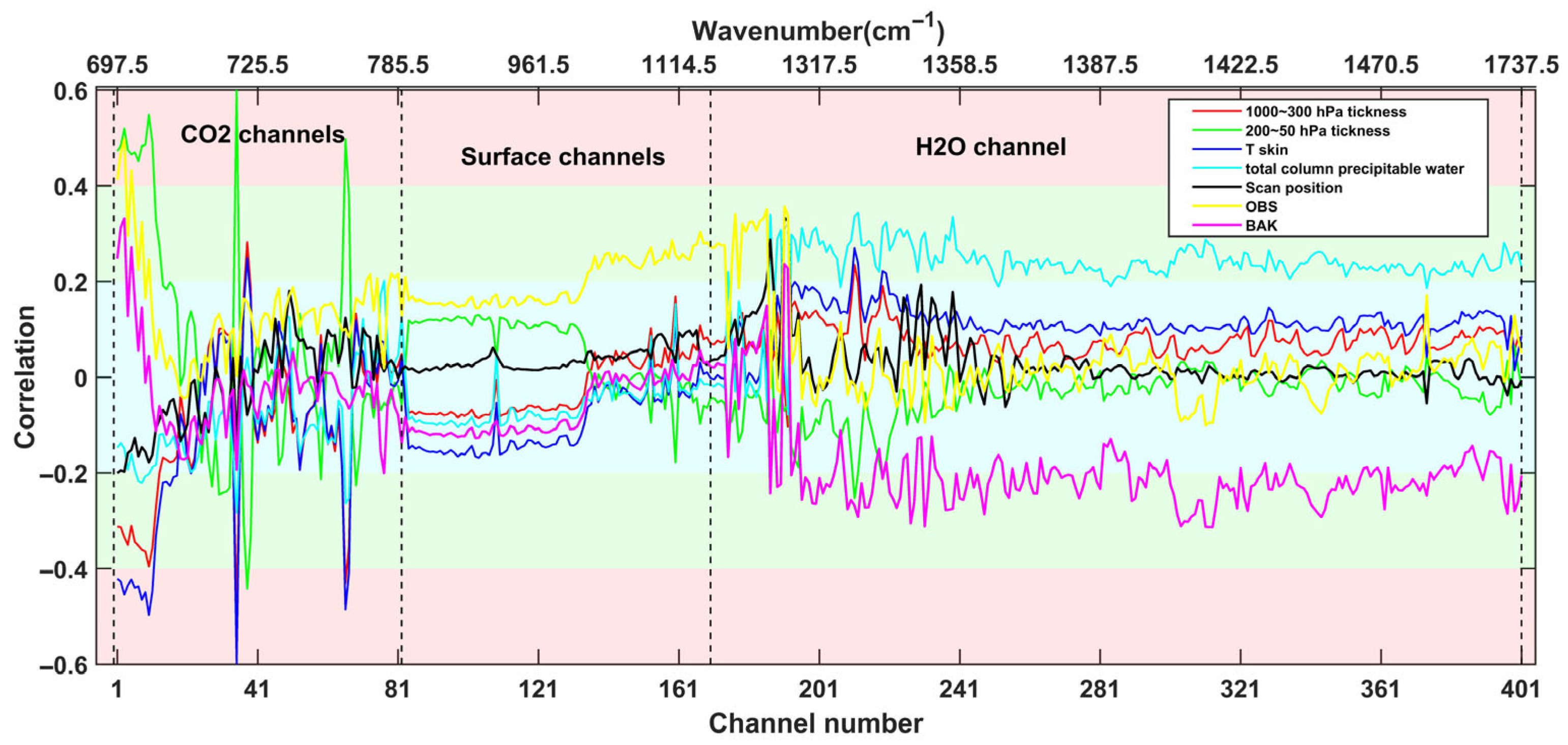
To investigate the correlation between the systematic biases in the FY-3E/HIRAS-II assimilated channels and the seven selected predictors, the Pearson correlation coefficients between each HIRAS-II channel O-B and each predictor are calculated (Figure 2). Data are collected from clear-sky FOVs over the ocean from 13 to 26 July 2023. The lower horizontal axis in Figure 2 is the serial number of the assimilated channels, and the upper horizontal axis is the wavenumber of the assimilated channels. The vertical coordinate is the Pearson correlation coefficient; the closer the value is to 1 (or −1), the higher the correlation. The solid lines with different colors represent different predictors. The blue shading indicates a low correlation (the correlation coefficient $\left|r\right|<0.2$), the green shading indicates a moderate correlation (the correlation coefficient $0.2\ll \left|r\right|<0.4$) and the red shading indicates a relatively high correlation (the correlation coefficient $0.4\ll \left|r\right|<0.6$). Figure 2 displays the fact that the biases of high-level longwave CO₂ channels 1–17 have relatively high correlation with 200–50 hPa thickness and model surface skin temperature, while the majority of the other CO₂ channels have a relatively low correlation (<0.2) with all predictors. For the window channels, the correlation coefficients of all predictors are relatively low, and basically within 0.2. The correlation coefficients between the water vapor channels and the predictors of model total column water vapor and simulated BT are moderate, while the correlation coefficient with other predictors is generally less than 0.2. It is worth noting that the O-B of high-level CO₂ channels correlate well with all predictors, including model skin temperature and even total column water vapor (although with the smallest value). Furthermore, the O-B of window channels show weak correlation with skin temperature. It is important to realize that the calculated correlation is between O-B and the predictors, not the radiances themselves. We are talking about the departure between observed and calculated background radiances. It does not necessarily follow that if a channel senses a given level of the atmosphere, the bias will depend on this level; it may come from another level altogether, due to correlations present in the background field [13]. It can be seen from Figure 2 that traditional linear BC schemes (e.g., static BC and variational BC) may not be able to completely eliminate the systematic biases in some specific FY-3E/HIRAS-II channels.

Figure 2. Correlation between O-B and predictors estimated from clear-sky data for the 401 assimilated channels. Different colored solid lines represent different predictors. The blue shading indicates a low correlation (the correlation coefficient $\left|\mathrm{r}\right|<0.2$), the green shading indicates a moderate correlation (the correlation coefficient $0.2\ll \left|\mathrm{r}\right|<0.4$) and the red shading indicates a relatively high correlation (the correlation coefficient $0.4\ll \left|\mathrm{r}\right|<0.6$).

The correlation between the FY-3E/HIRAS-II O-B and the selected predictors (Figure 2) shows that the linear correlation in some FY-3E/HIRAS-II channels does not indicate high correlation or significant relationships. The above schemes based on linear regression may lead to residual biases. XGBoost is an optimized Gradient Boosting Decision Tree (GBDT) algorithm whose core strengths include efficiency, flexibility and regularization ability in handling large-scale datasets. XGBoost uses second-order Taylor expansion in optimizing the loss function, which makes the algorithm more accurate in handling weak linear or nonlinear problems [22].

Therefore, this study establishes a BC scheme for FY-3E/HIRAS-II based on the XGBoost machine learning model. The XGBoost training data is FY-3E/HIRAS-II O-B and the predictors acquired from clear-sky FOVs over the ocean from 0000 UTC 13 to 1800 UTC 26 July 2023; all available samples within every 6 h assimilation window are used. The model input is model surface skin temperature, model total column water vapor, 1000–300 hPa thickness, 200–50 hPa thickness, scan position, observed BT, and simulated BT. The advantage of adding scan position is the elimination of the scan-angle BC, achieving both scan-angle BC and airmass BC in one step. The model output is FY-3E/HIRAS-II O-B. The total number of samples are 138,150 pairs; all samples are divided into 70% training data and 30% validation data. Data splitting is achieved by selecting three validation samples from every seven training samples, to ensure independence between training and validation sets. The 70% training data is used to train the model, while the other 30% subset is used to continuously adjust the hyperparameters of XGBoost, to obtain the optimal model. The model is tested using subsequent 14-day independent observations. The 401 separate channel-specific models are trained because the BT for each channel is different. The hyperparameters of XGBoost are continuously tuned and optimized through the metrics of Mean Absolute Error (MAE) and Root Mean Square Error (RMSE). The MAE and RMSE are computed as:

$$MAE={\displaystyle \frac{1}{N}}\sum _{n=1}^N\left|R_n^{test}-R_n^{pred}\right|$$

(11)

$$RMSE=\sqrt{{\displaystyle \frac{1}{N}}{\sum _{n=1}^N{(R}_n^{test}-R_n^{pred})}^2}$$

(12)

where $R_n^{test}$ is the truth from each sample of the testing data, and $R_n^{pred}$ is the corresponding prediction for each sample. Lower values of MAE and RMSE generally indicate that the model has better prediction ability. This article also uses the RMSE and MAE as criteria to select models. The RF (Random Forest) model is an ensemble learner comprising multiple decision trees, known for its high prediction accuracy and interoperability. The average RMSE of the validation set for the XGB model and RF model is 0.1736 and 0.6216, respectively. The average MAE for the XGB model and RF model is 0.1271 and 0.3782, respectively. Since the scheme is also a static BC scheme, the bias estimation needs to be updated frequently, so training time is also one of the factors worth considering. There is a significant difference in training time between the two models. It takes about 26 h for the RF model to train on the 12th Gen Intel Core i5-12400F CPU, while training the XGB model only takes 3.5 h. This is also the advantage of the XGB model in handling hyperspectral radiance data with large data volume.

4. Experiment Design and Results

Four parallel experiments are designed to examine the effect of different BC schemes on FY-3E/HIRAS-II DA. The first experiment (NOBC) is a control experiment that assimilates conventional data and FY-3E/HIRAS-II observations without BC. The second experiment (STC) assimilates conventional data and FY-3E/HIRAS-II observations with static BC. The third experiment (VAR) and the fourth experiment (XGB) are consistent with the second experiment, except using variational BC and XGBoost BC, respectively.

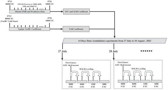
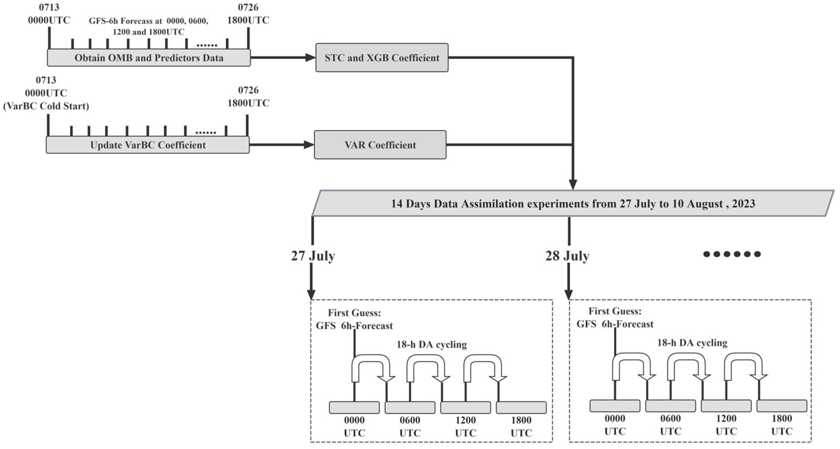
The complete experiment procedure is illustrated in Figure 3. The STC BC coefficients and XGB model are statistically trained, based on the offline O-B and predictors obtained from every assimilation time during the period 13 to 26 July 2023 (two weeks before the experiments). Due to the lack of FY-3E/HIRAS-II DA module in WRFDA, a variational BC cold-start method (i.e., the initial coefficients of each predictor are set to 0) is adopted, to train the variational BC coefficients for FY-3E/HIRAS-II in this article. The variational BC coefficients were cold-started at 0000 UTC 13 July 2023, and were continuously updated at each subsequent assimilation time from 0600 UTC 13 July to 1800 UTC 26 July 2023, to stabilize the coefficients. Then the variational BC coefficients updated after 14 days are applied to the subsequent assimilation experiments (27 July to 10 August 2023) and similarly updated at each assimilation time.

Figure 3. Schematic illustration of BC scheme establishment and the DA cycling experiments.

The 14-day assimilation experiments are conducted from 0000 UTC 27 July to 1800 UTC 10 August 2023. The detailed cycling assimilation procedure is shown in Figure 3. Each day, experiments with different BC schemes are all cold-started at 0000 UTC, using the GFS 6 h forecast data as the initial background field, and then cyclically consecutive assimilate observations at 0600, 1200, and 1800 UTC. The WRF-ARW V4.4 model 6 h forecast is used to generate the background field for the next assimilation time. The research domain for all experiments is approximately between 0°N~60°N and 70°E~150°E, as shown is Figure 1b. The domain is configured with 889 × 828 horizontal grids with a 9 km spatial resolution and 60 vertical levels up to 10 hPa.

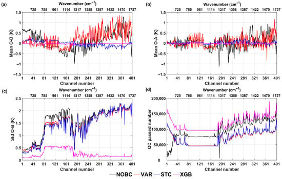
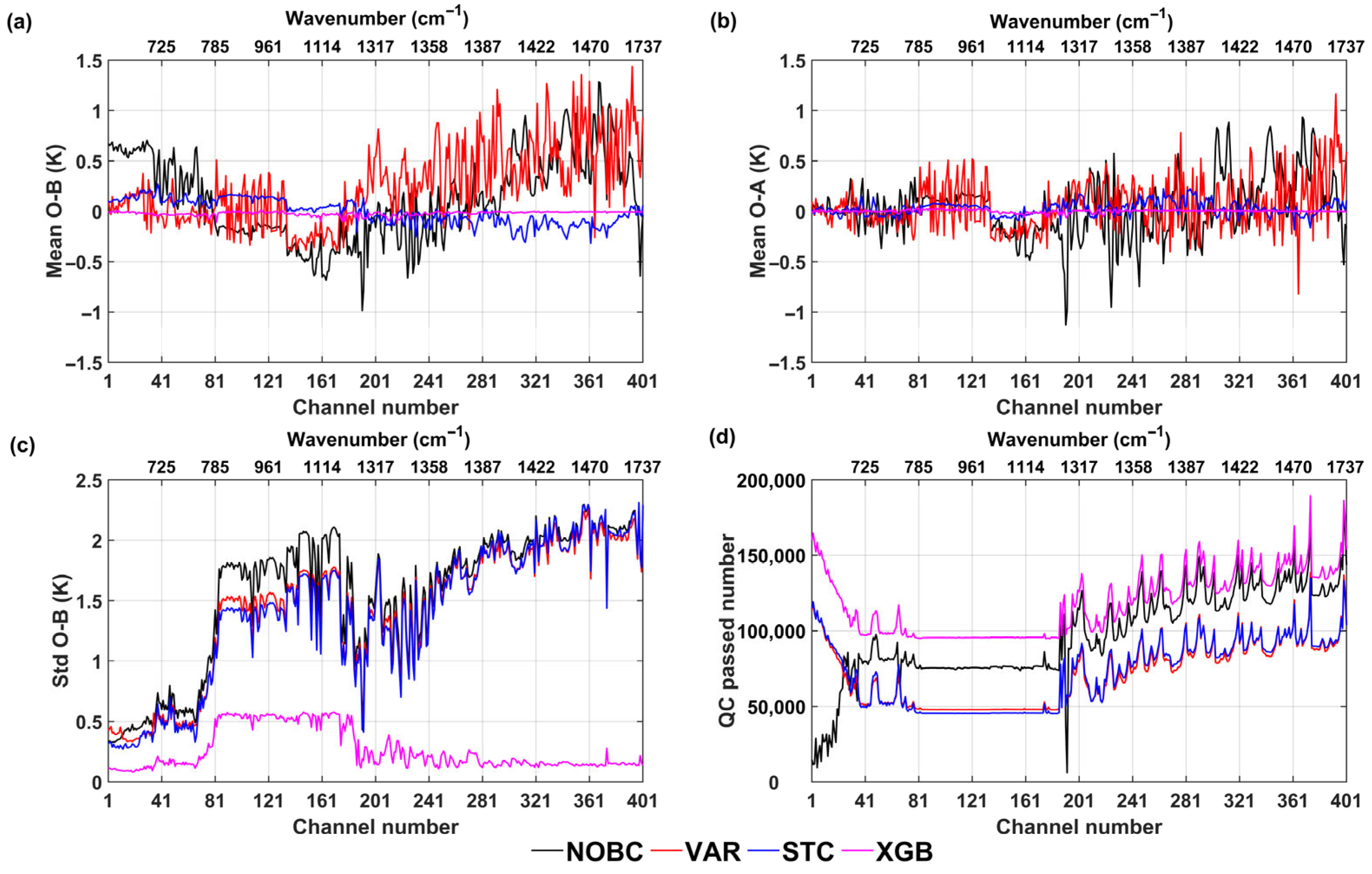
The impact of different BC schemes on the FY-3E/HIRAS-II DA is shown in Figure 4. Figure 4a,c,d illustrate the impact of different BC schemes before DA. The lower horizontal axes in Figure 4a,c,d are the serial numbers of the assimilated channels. The upper horizontal axes are the wavenumber of the assimilated channels, and the vertical axes are the mean O-B, the standard deviation of O-B, and the number of observations passing through QC, respectively. The solid lines with different colors represent different BC schemes. The black lines, and the red, blue and purple lines are the results of without BC VAR BC, STC BC and XGB BC, respectively. From Figure 4a, it can be seen that all BC schemes have obvious effects on the longwave CO₂ channels (No. 1~81). The XGB has the most significant correction effect, with the mean O-B in all longwave CO₂ channels approaching 0 after BC. There are still some residual biases after STC and VAR BC, and the mean O-B value of each channel is related to the correlation (Figure 2). The mean O-B gradually increases as the correlation decreases. The biases of window channels No. 82~134 have weak correlations (<0.2) with all predictors. There are still mean O-B biases of about 0.2 K in these channels after STC BC. After VAR BC, there are significant oscillations in the mean O-B, with a maximum of 0.5 K. The mean O-A of window channels No. 82~134 do not decrease in VAR BC. After XGB BC, both mean O-B and mean O-A in window channels No. 82~134 are generally around 0. For the near-surface channels No. 135~164, the mean O-B before BC and after STC and VAR BC are comparable, but the standard deviation of O-B is large (>1.5 K). Only the XGB has a mean O-B close to 0 and a standard deviation reduced to 0.5 K, followed by the STC. For the water vapor channels (No. 175~401), the mean O-B and standard deviations (about 2 K) before BC and after VAR BC are large, and increase slightly with decreasing peak heights of the weight function. The biases of water vapor channels No. 262~401 are not completely eliminated after VAR and STC BC, and the standard deviations are also not significantly improved. This may be related to the weak correlation with the used predictors (the total column water vapor is around 0.2, and the other predictors are less than 0.2). The mean O-B after XGB BC stabilizes near 0, with a standard deviation below 0.2 K. It can be seen from Figure 4d that more observations pass QC (quality control) after XGB BC, but not after STC and VAR BC. The effect of different BC schemes on the assimilated analysis is shown in Figure 4b. The analysis biases become smaller for all BC schemes after assimilation compared to Figure 4a, especially for the CO₂ channels at a large height. The mean O-A of XGB is the smallest, approaching 0 K. Overall, it is unclear whether the mean and standard deviation of O-B or the mean O-A are the smallest for XGB and the second smallest for STC in all channels.

Figure 4. (a) Mean O-B, (b) mean O-A, (c) O-B standard deviation, and (d) the number of data which passed QC, counted from experiments from 27 July to 10 August 2023. (Only data that passed the QC process are used. Different colored solid lines represent different BC schemes).

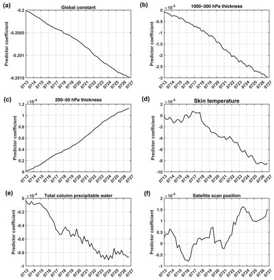
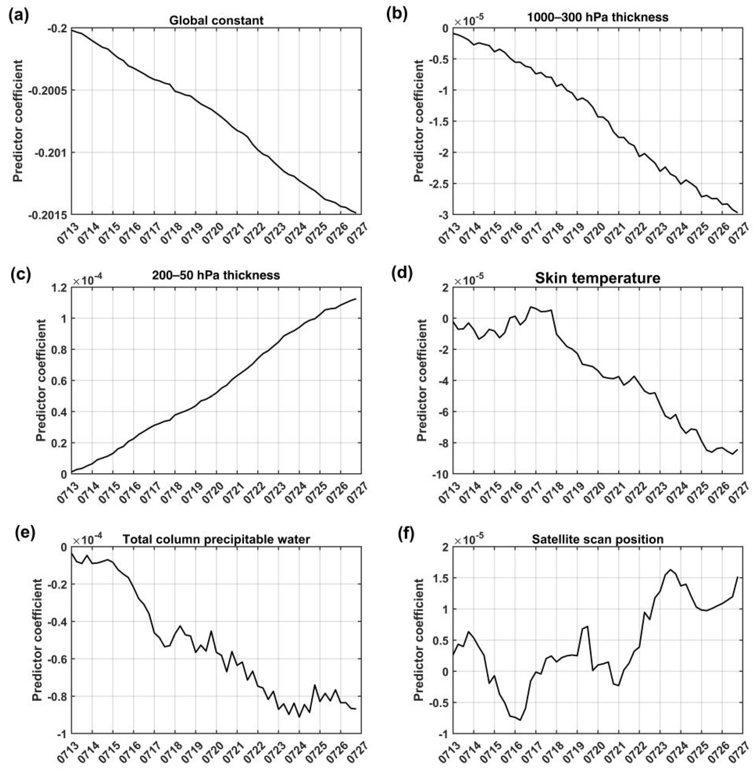
There is currently no FY-3E/HIRAS-II DA module within WRFDA V4.5.1, and no reference variational BC coefficients as with other mature instruments. Therefore, the FY-3E/HIRAS-II variational BC coefficients are trained by cold-start, referring to the WRFDA users’ guide. The evolution of variational BC coefficients in channel 263 (1375 cm⁻¹) are shown in Figure 5. Figure 5a–f show the coefficients evolution of 1000–300 hPa thickness, 200–50 hPa thickness, model surface skin temperature, model total column water vapor and scan position, respectively. The horizontal axes represent the assimilation time, and the vertical axes represent the coefficients. When WRFDA variational BC cold-start (00UTC 13 July), the coefficient of constant is set to the mode of the O-B samples in this channel, and the coefficients of the other predictors evolve from 0. As can be seen from the vertical axis of Figure 5, the magnitude of the different variable coefficients varies greatly. The coefficient of constant is close to −0.2 (Figure 5a), while the coefficients of the other five predictors (Figure 5b–f) are with a magnitude of the order of 10⁻⁴ and 10⁻⁵. That is to say, all these coefficients evolve very slowly during the assimilation cycle and the constant term plays an absolutely dominant role. As a result, only the constant predictor with slow evolution contributes significantly during actual DA experiments, which may result in the poor performance of the VAR BC scheme. Currently, only the intuitive evolution of variational coefficient update in the system is presented, and its physical mechanism requires further analysis in the future. A preliminary guess is that, due to the characteristics of HIRAS-II hyperspectral observations, each channel only contains radiance information from a very thin layer of the atmosphere (the weight-function response range of infrared instruments is much narrower than that of microwave instruments), while predictors such as 1000–300 thickness, 200–50 thickness, and total column water vapor represent information from considerably thicker atmospheric layers. Therefore, each channel can only make minor adjustments to the atmospheric state parameters of a very thin layer after assimilation, which may not be able to be fed back into these predictors representing considerably thicker atmospheres. Additionally, the weak linear correlations between the selected predictors and biases are also the reason why VarBC degrades to a constant-only correction.

Figure 5. Time series of the variational coefficients for (a) constant, (b) 1000–300 hPa thickness, (c) 200–50 hPa thickness, (d) model surface skin temperature, (e) model total column water vapor and (f) scan position, from 13 to 26 July 2023. The background constraint parameter “VARBC_NBGERR” is set to 2000.

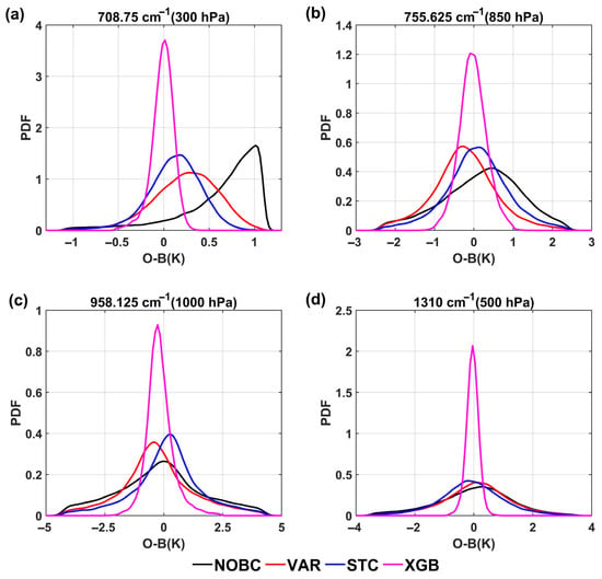
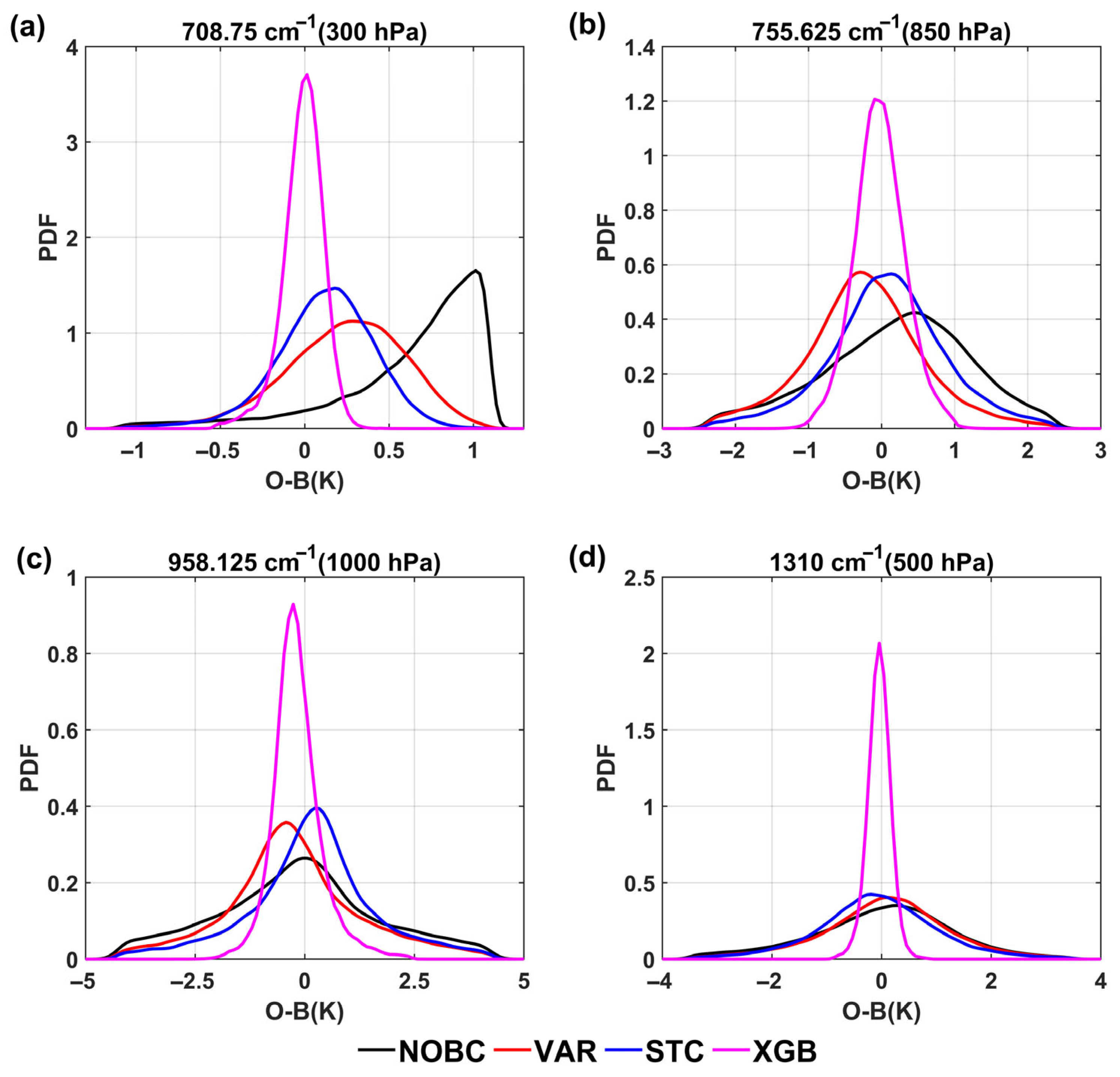
A core objective of bias correction is to make the O-B distribution unbiased and Gaussian. The results with probability density function (PDF) plots of O-B (before and after correction) for representative channels (two CO₂ channels, one window channel and one H₂O) are shown in Figure 6. Figure 6a–d show the results of the CO₂ channel with a wavenumber of 708.75 cm⁻¹ (the peak height of weight function is 850 hPa), the CO₂ channel with a wavenumber of 755.625 cm⁻¹ (the peak height of weight function is 500 hPa), the window channel with a wavenumber of 958.125 cm⁻¹, and the water vapor channel with a wavenumber of 1310 cm⁻¹ (the peak height of weight function is 500 hPa), respectively. The horizontal axes represent the value of O-B, and the vertical axes represent the PDF. The different color lines are different BC schemes. For 708.75 cm⁻¹ channel (Figure 6a), the O-B distribution exhibits a pronounced negative skewness before BC; the degree of negative skewness is reduced but still present after STC and VAR BC. After XGB BC, the overall distribution conforms to a Gaussian distribution with a mean of 0, but there are still some biases in the left tail that have not been eliminated. The O-B distributions of the 755.625 cm⁻¹ channel and 1310 cm⁻¹ channel are more consistent with Gaussian after BC, but there are still certain biases after VAR and STC BC. The O-B of the two channels after XGB BC follow unbiased Gaussian distributions. Figure 6c indicates that the window channel exhibits a slight positive skew after XGB BC. The standard deviations of O-B for all channels have significantly decreased, and effectively center the distribution around zero after XGB BC.

Figure 6. The probability density function (PDF) of O-B for (a) the 708.75 cm⁻¹ channel, (b) the 755.625 cm⁻¹ channel, (c) the 968.125 cm⁻¹ channel and (d) the 1310 cm⁻¹ channel before and after BC, from 27 July to 10 August 2023.

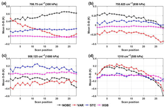
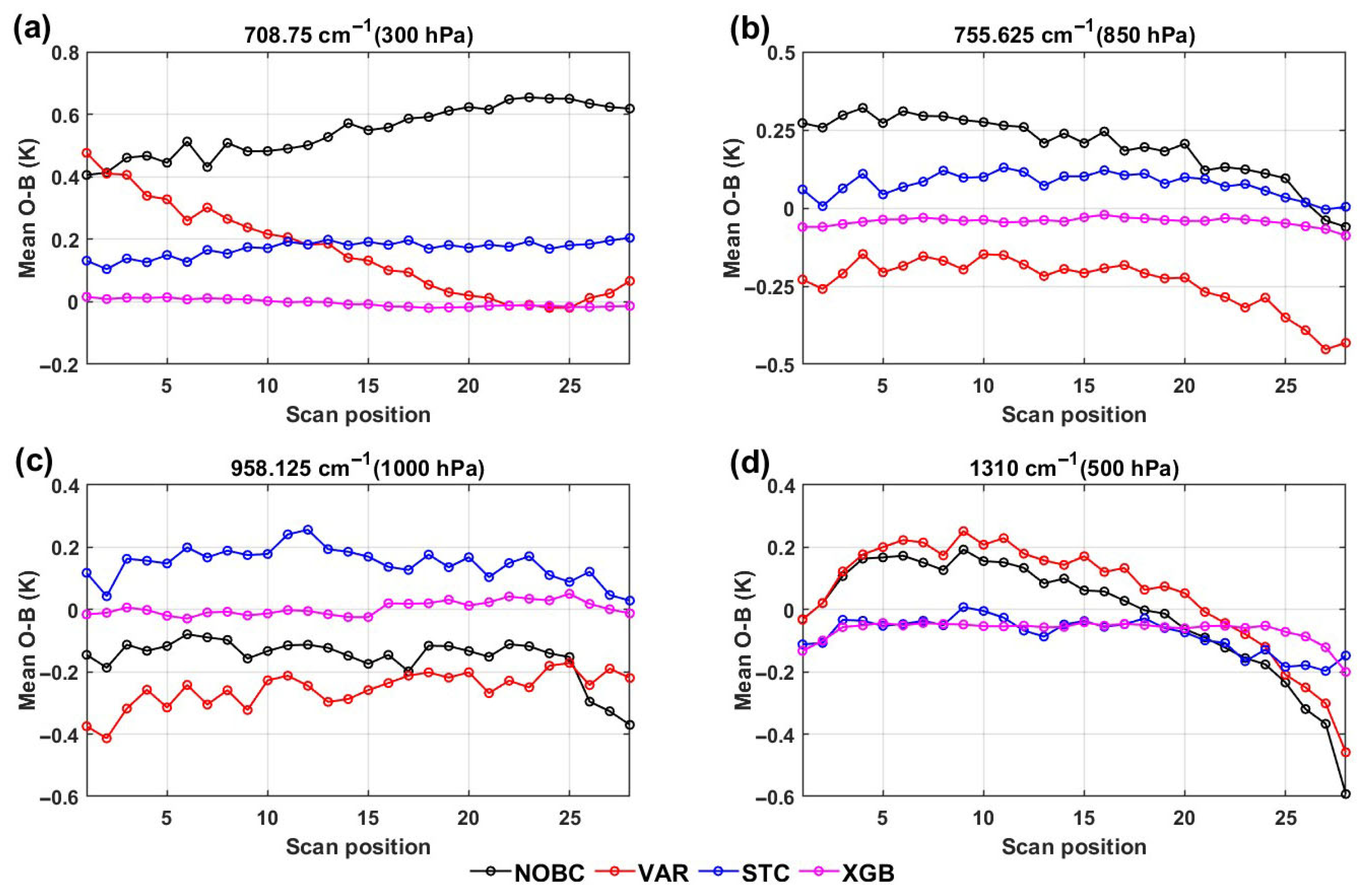
The FY-3E/HIRAS observations suffer from obvious scanning biases. The STC BC implements a scan-angle BC based on the pre-computed, position-specific scan BC coefficients. The VAR BC adds the scan position as predictors; their coefficients are updated during the minimization process to quantitatively correct scan biases. The XGB BC also attempts to eliminate the lime effect by using the scan position as one of predictors. It is necessary to demonstrate the correction effects of different BC schemes on scan biases. Figure 7 shows the scan variations of O-B biases before and after BC for four representative channels (the same as in Figure 6). The horizontal axes are the scan positions, and the vertical axes are the mean O-B. The different lines indicate different BC schemes. The mean O-B shows obvious scan-dependent biases for all channels (black lines). The scan-dependent biases are not eliminated after VAR BC (red lines), which may be caused by the failure of VAR BC. In general, the mean O-B are reduced after STC and XGB BC. However, there are residual scan-dependent biases after STC BC (blue lines). The XGB BC scheme (purple lines) performs better in reducing the scan-dependent biases, especially for the 708.75 cm⁻¹ channel (Figure 7a).

Figure 7. The scan variations of O-B for (a) the 708.75 cm⁻¹ channel, (b) the 755.625 cm⁻¹ channel, (c) the 968.125 cm⁻¹ channel and (d) the 1310 cm⁻¹ channel before and after BC, from 27 July to 10 August 2023.

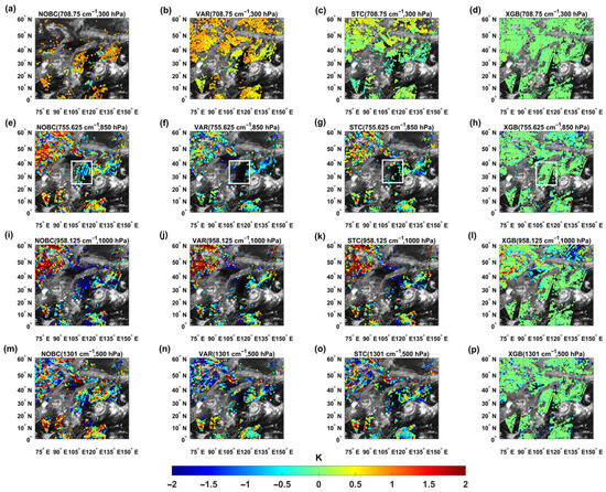
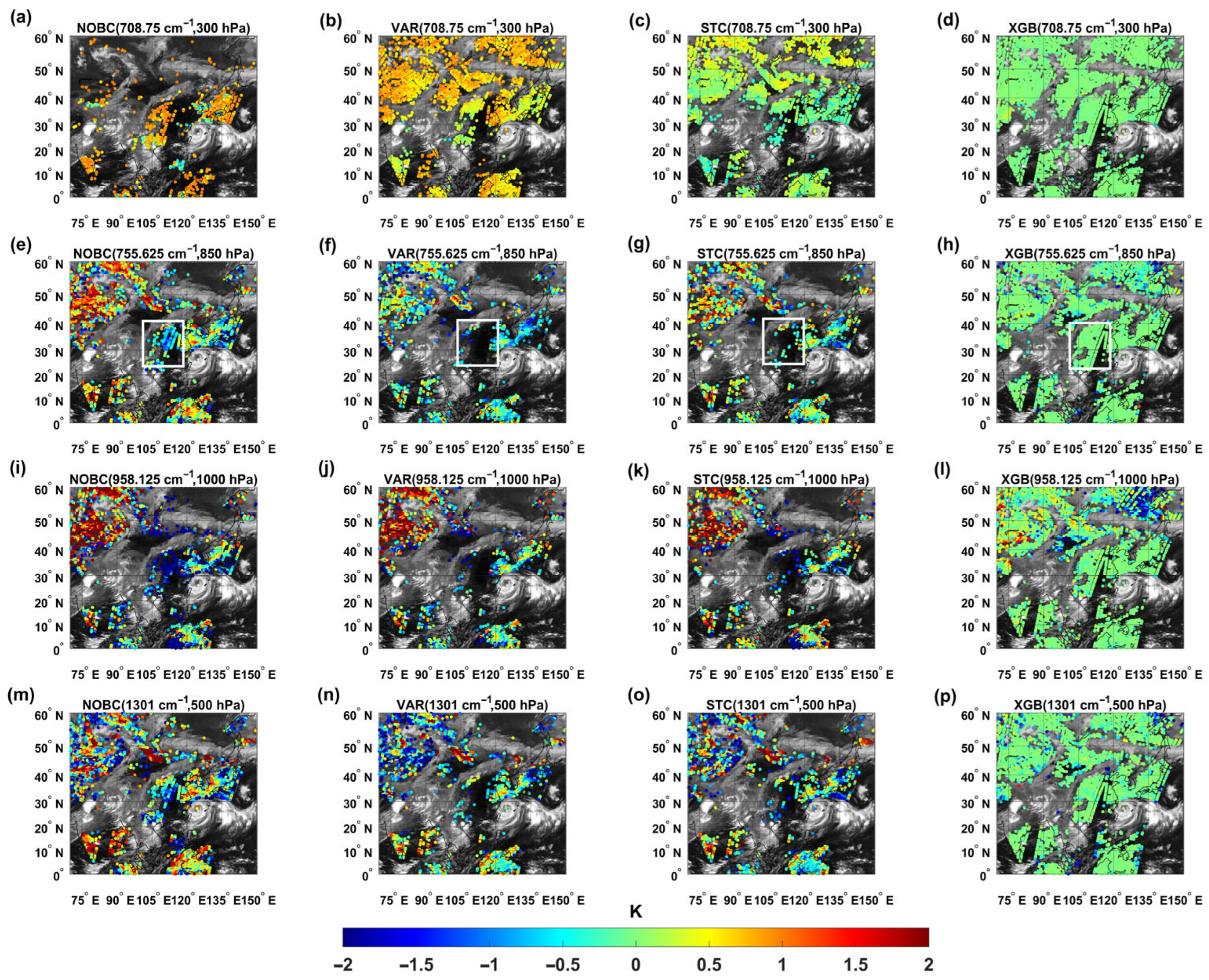
Figure 8 shows the bias distribution of different BC schemes at 0000 UTC 4 August 2023. The first-to-fourth column subplots show the results of the NOBC, VAR, STC and XGB, respectively. The first-to-fourth rows represent the temperature channel with a central wavenumber of 708.75 cm⁻¹ (the peak height is 300 hPa), the temperature channel with a central wavenumber of 755.625 cm⁻¹ (850 hPa), the window channel with a central wavenumber of 955.125 cm⁻¹ (1000 hPa), and the water vapor channel with a central wavenumber of 1310 cm⁻¹ (500 hPa), respectively. The colors in all subplots represent the O-B value of the FOVs, and the black shading is a cloud image displayed by FY-4A/AGRI longwave-infrared window channel observations. Figure 8a–d shows the O-B distribution in a CO₂ channel with a higher peak weight function, which is mainly used for remote sensing of temperatures near 300 hPa. It can be seen that all BC schemes have obvious correction effects in the channel, compared with NOBC (Figure 8a), and more observations are assimilated due to the reduction in O-B. XGB has the most significant correction effect. For the temperature channel at 850 hPa (Figure 8e–h), the number of observations assimilated decreases relative to the high channel, especially over the cloudy and surrounding region. Although the O-B was reduced in all BC schemes, the number of observations assimilated after STC and VAR BC is significantly reduced, as shown in the white rectangles in Figure 8e–h. It can be seen from the cloud image that the region is a clear-sky area, originally with a small O-B (−1~0.5 K); in these, FOVs increase after the VAR and STC BC, resulting in some valid observations unable to pass QC. This is probably due to the low correlation between the predictors and the O-B in this channel. The results in the window channel are shown in Figure 8i–l. The overall biases are not significantly decreased after STC and VAR BC. Most of the biases are eliminated after XGB BC, but there are still some biases in high-latitude regions. Figure 8m–p show the results in a water vapor channel at 500 hPa. Similarly, the biases are smallest after XGB BC, thus allowing most observations to pass QC. Some effective observations are discarded after VAR and STC BC.

Figure 8. Spatial distributions of the HIRAS-II O-B for NOBC (a,e,i,m), VAR (b,f,j,n), STC (c,g,k,o) and XGB (d,h,l,p) for (a–d) 708.75 cm⁻¹ channel (300 hPa), (e–h) 755.625 cm⁻¹ channel (850 hPa), (i–l) 958.125 cm⁻¹ channel (1000 hPa) and (m–p) 1310 cm⁻¹ channel (500 hPa) at 0000 UTC 4 August 2023. The black shading indicates the observed FY-4A AGRI BT of the window channel 13 with a central wavelength of 12 µm.

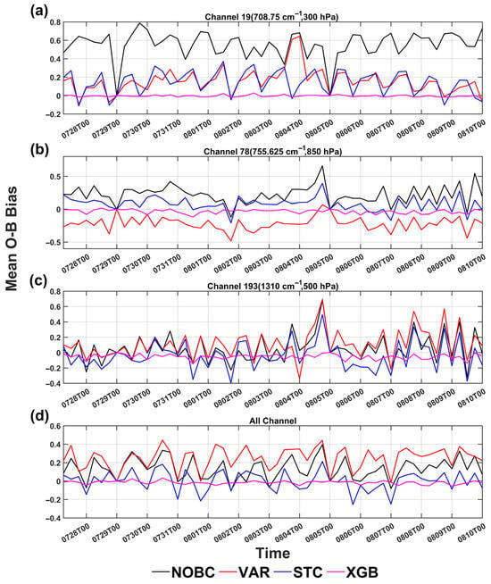
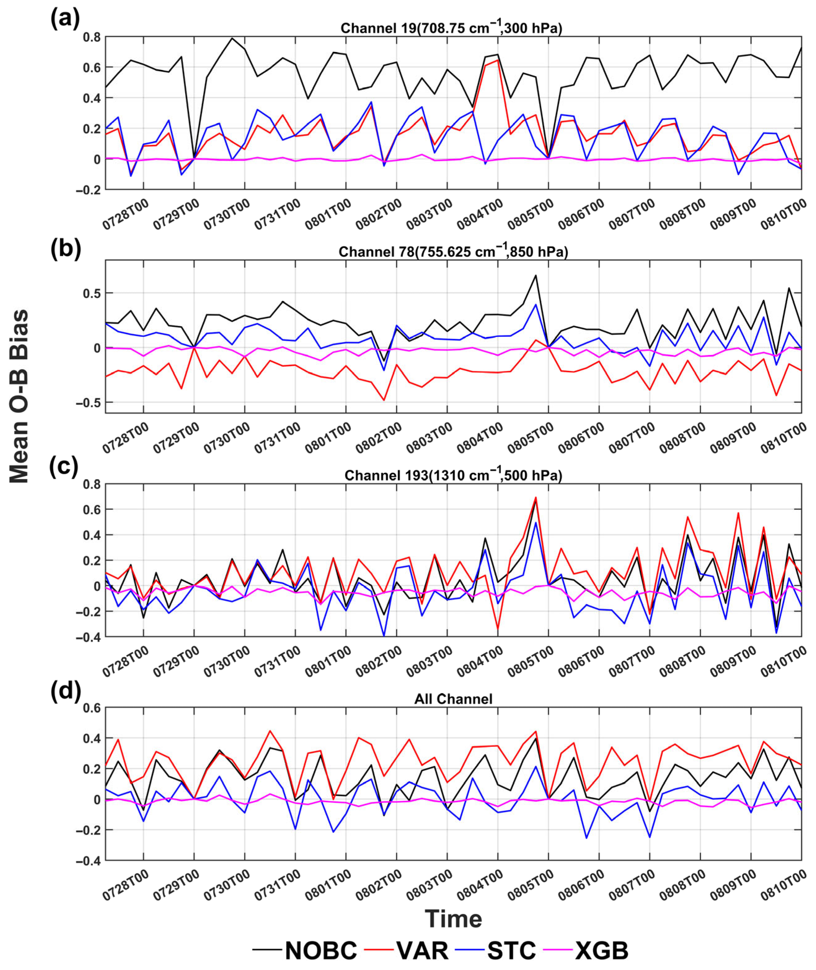
The STC and XGB are essentially offline BC, so it is necessary to verify the stability in long-term assimilation experiments. The change in mean O-B with time for different BC schemes is shown in Figure 9. The horizontal axis represents assimilation time, and the vertical axis is mean O-B. The solid lines with different colors represent different BC schemes. Figure 9a–d are the results in channels with a wavenumber of 708.75 cm⁻¹, 755.625 cm⁻¹, and 1310 cm⁻¹, and the average of all channels, respectively. It can be seen from Figure 9a that the correction effects of all schemes are quite significant (the O-B was significantly reduced). However, the mean biases do not change much before and after STC and VAR BC, with the channel heights decreasing, especially for the water vapor channel (Figure 9c). This is mainly due to the weaker correlation between the O-B and predictors in these water vapor absorption bands. The mean O-B values still fluctuate over time after VAR and STC BC, for whole channels (Figure 9d). The XGB scheme is the most stable, with the biases approaching 0, followed by the STC scheme.

Figure 9. Time series of the mean O-B for different bias-correction experiments for (a) the 708.75 cm⁻¹ channel (300 hPa), (b) the 755.625 cm⁻¹ channel (850 hPa), (c) the 1310 cm⁻¹ channel (500 hPa) and (d) all channels, from 27 July to 10 August 2023.

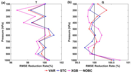
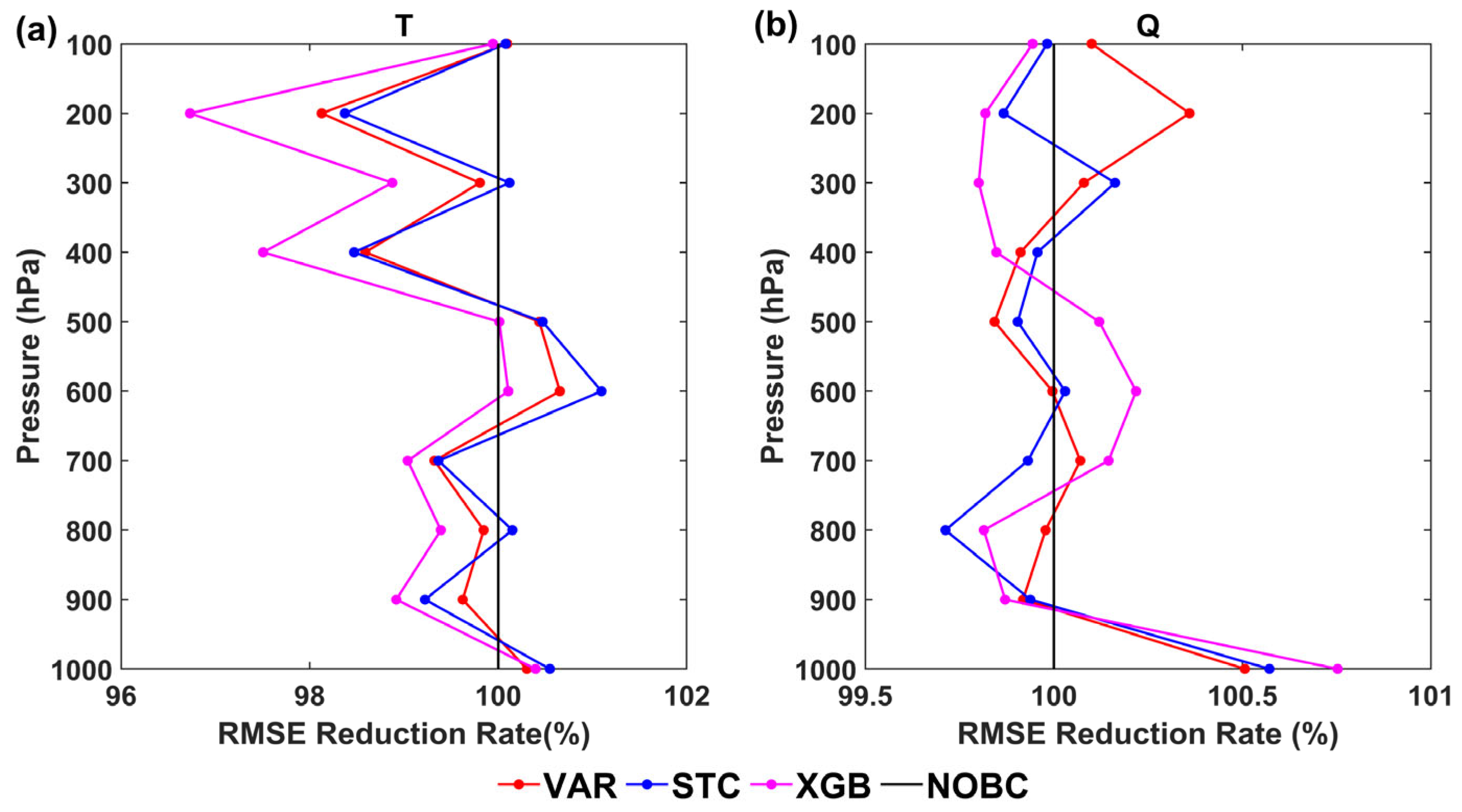
Independent ERA5 objective analysis fields are selected as the truth to further evaluate the impact of different BC schemes on the DA analysis fields, because the GFS 6 h forecast data are used as the first guess in all assimilation experiments. The analysis fields with different BC schemes for a total of 56 assimilation times from 27 July to 10 August 2023 are compared with ERA5. Figure 10a,b show the vertical RMSE profiles normalized by the experiment NOBC. The horizontal axis is the RMSE variation relative to experiment NOBC. The value less than 100% indicates a decrease in RMSE (the analysis field is improved) after BC, and the value greater than 100% means the RMSE increases (the analysis field is not improved). Figure 10a indicates that the temperature analysis fields in the upper and lower levels are effectively improved after BC. XGB reduced the temperature RMSE at 200 hPa by approximately 3.8% (from 0.78 K to 0.75 K) compared to NOBC, which was a larger reduction than that achieved by Static BC (1.6%) or Var BC (1.8%). The XGB scheme is the most significant improvement among these three schemes, especially in the upper-temperature analysis fields. From Figure 10b, all BC schemes show slight variations in the water vapor analysis fields relative to NOBC, with changes in RMSE within 0.3%. Figure 4 shows excellent O-B correction for water vapor channels, yet Figure 10b shows minimal impact (~0.3% RMSE change) on the analyzed humidity fields. The radiance received by the water vapor absorption band is not only related to the water vapor content in the atmosphere, but also to temperature. Furthermore, the water vapor content changes rapidly and significantly over time and space, making it difficult for observations within a 6 h assimilation window to respond in a timely manner. Additionally, it may be due to the relatively large observation errors in the HIRAS-II water vapor channels and lower weight given to humidity fields in the background error covariance. Further research will be conducted in the future.

Figure 10. Averaged vertical RMSE profiles (normalized by the RMSE from the NOBC experiment) of (a) temperature and (b) water vapor compared with ERA5.

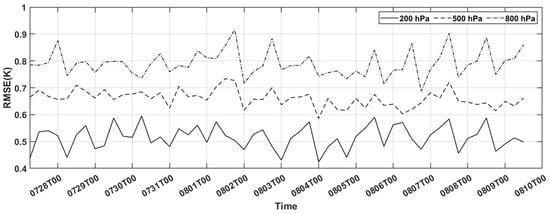
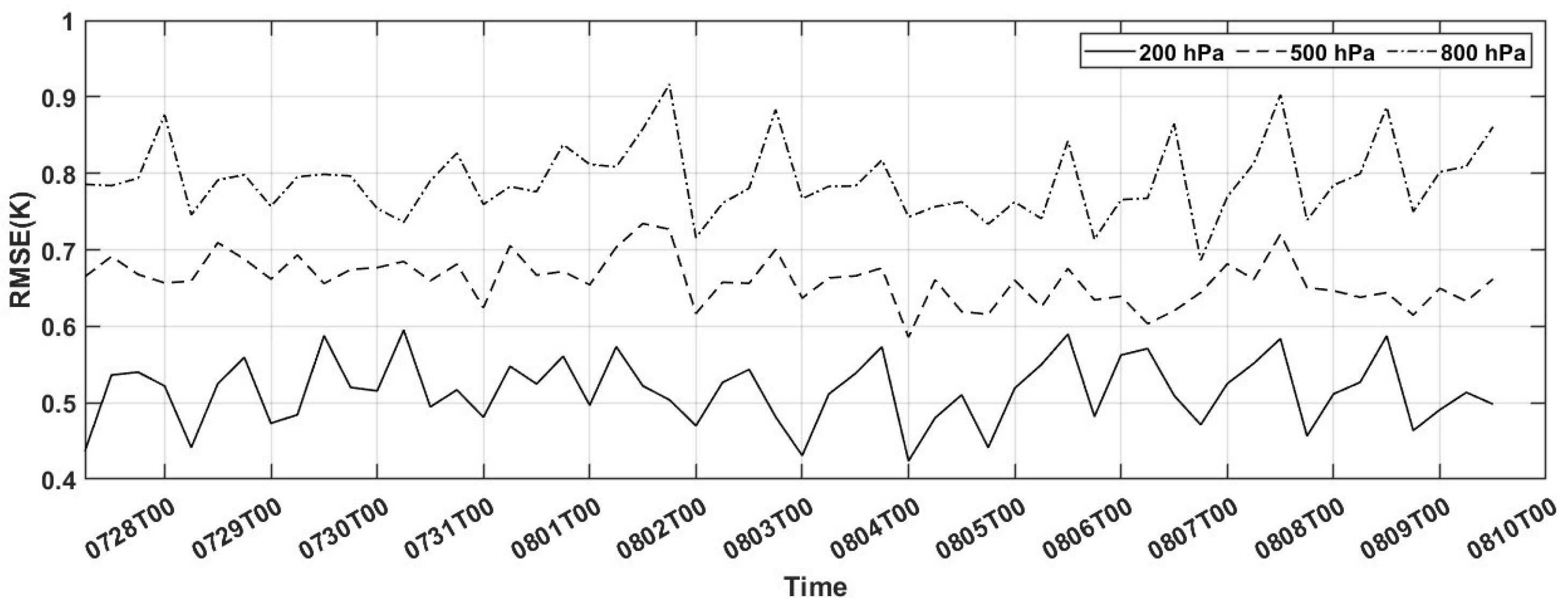
Figure 11 shows the RMSE variation of the XGB scheme temperature analysis over time at different height levels. The horizontal axis is the assimilation time and the vertical axis is RMSE. Solid, dashed and dotted lines represent the level at 200 hPa, 500 hPa and 800 hPa, respectively. It is obvious from Figure 11 that the temperature RMSE of different heights remains relatively stable over a long period. The analysis field gets closer to the ERA5 as the height increases. The observation error of the 703.75 cm⁻¹ channel (200 hPa), 726.875 cm⁻¹ channel (500 hPa) and 753.75 cm⁻¹ channel (800 hPa) is 0.17 K, 0.25 K and 0.32 K, respectively. The variation in RMSE with time for different height layers is within 0.1 K, indicating that the XGB model in the experimental region is robust during the cycling assimilation.

Figure 11. Time series of the temperature RMSE for XGB experiments at (solid line) 200 hPa, (dash line) 500 hPa and (dotted line) 800 hPa, from 27 July to 10 August 2023.

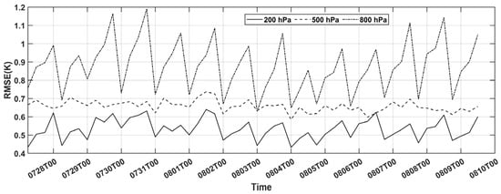
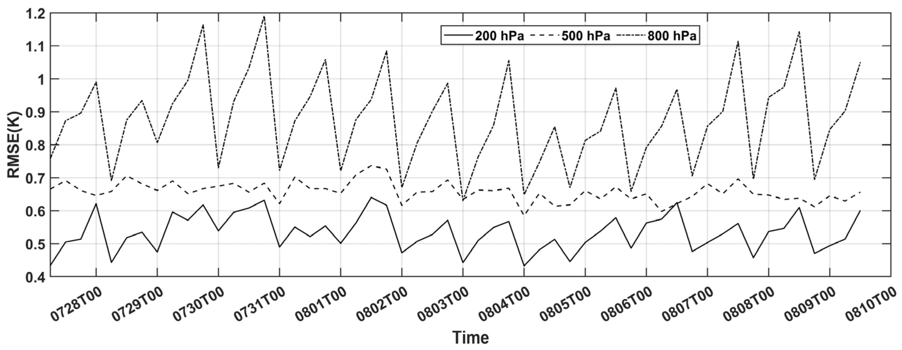
The temperature RMSE time series of the NOBC experiments are shown in Figure 12, in order to compare them with the XGB experiments. The temperature RMSE at 200 hPa and 800 hPa shows a growing trend and larger oscillations compared with the XGB experiments, especially at 800 hPa, with a maximum change approaching 0.5 K. The RMSE variation at 200 hPa is within 0.2 K, while it is comparable to that of XGB experiments at 500 hPa. The XGB scheme maintains stable analysis quality over time, and it shows more stable or non-deteriorating performance, relative to the NOBC experiments.

Figure 12. As in Figure 11, but for the NOBC experiments.

5. Conclusions

Three different BC schemes including a new machine learning XGBoost scheme for the FY-3E/HIRAS-II radiance observations based on innovation O-B from 13 to 26 July 2023 are established in this article. The impact of different BC schemes on FY-3E/HIRAS-II DA is objectively evaluated through two-week DA experiments from 27 July to 10 August 2023. The main conclusions are as follows:

(1)

Among the three BC schemes (static BC, variational BC and XGBoost BC), the XGBoost BC is the most effective in correcting O-B. The mean and standard deviation of O-B in all HIRAS-II channels are the smallest after XGB BC, followed by the STC BC. The correction amount for O-B in all schemes gradually decreases as the channel detection height decreases.

(2)

Since the static BC and the variational BC schemes are linear regression correction in nature, the nonlinear biases cannot be eliminated completely, especially for these HIRAS-II assimilated channels with which O-B has a weak correlation with correction predictors. The O-B of these channels are still large after BC, and lead to the loss of some valid observations.

(3)

The variational BC coefficients evolution proceeds slowly in longtime assimilation experiments. Except for the constant predictor, the other predictors have no significant effect. Preliminary research indicates that variational BC is not applicable to HIRAS-II.

(4)

The BC scheme based on XGBoost can effectively eliminate the linear and nonlinear biases of FY-3E/HIRAS-II observations. The mean values of O-B after XGB BC are near 0 and remain stable over a long time, which demonstrates its strong robustness. The computational efficiency of the XGBoost scheme is comparable to the static BC scheme, and faster than the variational BC scheme.

(5)

Compared with the independent ERA5 analysis fields, the RMSE of temperature analysis fields for the XGB scheme is the smallest at all levels, and the root mean square errors do not change much over time. this indicates that the improved bias correction translates into a persistently more accurate atmospheric analysis, which is the ultimate goal for improving NWP initial conditions.

A key finding from this study is that the predictors designed for broad atmospheric layers (e.g., 1000–300 thickness, 200–50 thickness, and total column water vapor) may be inadequate for hyperspectral instruments that sense very thin layers. There are many infrared hyperspectral instruments that have been assimilated operationally now, such as AIRS (Atmospheric Infrared Sounder), IASI (Infrared Atmospheric Sounding Interferometer) and CrIS (the Cross-track Infrared Sounder). Therefore, it is of potential significance to select new predictors specifically for hyperspectral infrared data, which may also improve the effect of Var BC. Despite the promising results mentioned above, there are still deficiencies and limitations. The training data is sourced exclusively from clear-sky oceanic FOVs, and the uncertainty of land surface emissivity and skin temperature might affect the model’s generalizability. This article primarily investigates the impact of different BC schemes on the assimilation of FY-3E/HIRAS-II radiance data. The deficiencies in channel selection and quality control have led to suboptimal results in the direct assimilation of FY-3E/HIRAS-II radiance data. For instance, the study region includes Western China, which features complex underlying surfaces with highly variable infrared surface emissivity, while a fixed surface emissivity value of 0.98 (default) is used in RTTOV. Although the bias estimation includes the RTTOV simulation error, the final results indicate that the biases have not been completely eliminated (Figure 6c). There is potential for improving assimilation effects (and BC effects in window channels) through implementing a quality control (QC) step to reject pixels over terrain with large emissivity variability. In addition, typically, only the long-wave HIRAS-II channels are assimilated operationally. To verify the impact of different BC schemes on the remaining channels (which may be assimilated in the future), a total of 401 HIRAS-II channels are assimilated in this study. However, the observation error covariance matrix used is diagonal, and the correlation between channels may lead to suboptimal assimilation effects for HIRAS-II. Due to space limitations, this study only discusses the impact of different bias corrections on the assimilation analysis field. The subsequent companion paper will continue to explore its influence on the numerical weather forecasts.

References

- Liu, Z.Q.; Zhang, F.Y.; Wu, X.; Xue, J.S. A regional ATOVS radiance-bias correction scheme for radiance assimilation. Acta Meteorol. Sin. 2007, 1, 113–123. (In Chinese) [Google Scholar] [CrossRef]
- Li, X.; Zou, X.; Zeng, M. An Alternative Bias Correction Scheme for CrIS Data Assimilation in a Regional Model. Mon. Weather Rev. 2019, 147, 809–839. [Google Scholar] [CrossRef] [Scilit]
- Zhang, P.; Hu, X.Q.; Sun, L.; Xu, N.; Chen, L.; Zhu, A.J.; Lin, M.Y.; Lu, Q.F.; Yang, Z.D.; Yang, J.; et al. The On-Orbit Performance of FY-3E in an Early Morning Orbit. Am. Meteorol. Soc. 2024, 105, 144–175. [Google Scholar] [CrossRef] [Scilit]
- Auligné, T.; McNally, A.P.; Dee, D.P. Adaptive bias correction for satellite data in a numerical weather prediction system. Q. J. R. Meteorol. Soc. 2007, 133, 631–642. [Google Scholar] [CrossRef] [Scilit]
- Auligné, T. An objective approach to modelling biases in satellite radiances: Application to AIRS and AMSU-A. Q. J. R. Meteorol. Soc. 2007, 133, 1789–1801. [Google Scholar] [CrossRef] [Scilit]
- Dee, D.; Uppala, S. Variational bias correction of satellite radiances data in the ERA-Interim reanalysis. Q. J. R. Meteorol. Soc. 2009, 135, 1830–1841. [Google Scholar] [CrossRef] [Scilit]
- Eyre, J.R. A Bias Correction Scheme for Simulated TOVS Brightness Temperatures; Technical Memorandum; ECMWF: Reading, UK, 1992; Volume 186, 34p. Available online: https://discover.library.noaa.gov/discovery/fulldisplay/alma991000723769707381/01NOAA_INST:NOAA (accessed on 20 February 2026).
- Hocking, J.; Rayer, P.; Rundle, D.; Saunders, R. RTTOV v12 User Guide; NWP SAF: Reading, UK, 2019; Available online: https://www.nwpsaf.eu/site/software/rttov/documentation/ (accessed on 20 February 2026).
- Zou, X.L. Atmospheric Satellite Observations: Variation Assimilation and Quality Assurance; Academic Press: San Diego, CA, USA, 2020; 388p. [Google Scholar] [CrossRef] [Scilit]
- Di, D. Data Assimilation Research for Geosynchronous Interferometric Infrared Sounder Onboard FengYun-4 Satellite. Ph.D. Thesis, Chinese Academy of Meteorological Sciences, Beijing, China, 2019. [Google Scholar]
- Yin, R.Y.; Han, W.; Gao, Z.Q.; Di, D. The evaluation of FY4A’s Geostationary Interferometric Infrared Sounder (GIIRS) long-wave temperature sounding channels using the GRAPES global 4D-Var. Q. J. R. Meteorol. Soc. 2020, 146, 1459–1476. [Google Scholar] [CrossRef] [Scilit]
- Harris, B.A.; Kelly, G. A satellite radiance-bias correction scheme for data assimilation. Q. J. R. Meteorol. Soc. 2001, 127, 1453–1468. [Google Scholar] [CrossRef] [Scilit]
- Uppala, S.; Kallberg, P.; Simmons, A.; Andrae, U.; Bechtold, V.D.C.; Fiorino, M.; Gibson, J.K.; Haseler, J.; Hernandez, A.; Kelly, G.A.; et al. The ERA-40 re-analysis. Q. J. R. Meteorol. Soc. 2005, 131, 2961–3012. [Google Scholar] [CrossRef] [Scilit]
- Derber, J.C.; Wu, W.S. The use of TOVS cloud-cleared radiances in the NCEP SSI analysis system. Mon. Weather Rev. 1998, 126, 2287–2299. [Google Scholar] [CrossRef] [Scilit]
- Dee, D. Variational bias correction of radiance data in the ECMWF system. In Proceedings of the ECMWF Workshop on Assimilation of High Spectral Resolution Sounders in NWP, Reading, UK, 26 June–1 July 2004; ECMWF: Reading, UK, 2004; Available online: https://www.ecmwf.int/sites/default/files/elibrary/2004/8930-variational-bias-correction-radiance-data-ecmwf-system.pdf (accessed on 20 February 2026).
- Zhu, Y.; Derber, J.; Collard, A.; Dee, D.P.; Treadon, R.; Gayno, G.; Jung, J.A. Enhanced radiance bias correction in the National Centers for Environmental Prediction’s Gridpoint Statistical Interpolation data assimilation system. Q. J. R. Meteorol. Soc. 2014, 140, 1479–1492. [Google Scholar] [CrossRef] [Scilit]
- Otkin, J.A.; Potthast, R.; Lawless, A.S. Nonlinear bias correction for satellite data assimilation using Taylor series polynomials. Mon. Weather Rev. 2018, 146, 263–285. [Google Scholar] [CrossRef] [Scilit]
- Zhang, X.W.; Xu, D.; Min, J.; Li, H.; Shen, F.; Lei, Y. A Machine Learning-Based Bias Correction Scheme for the All-Sky Assimilation of AGRI Infrared Radiances in a Regional OSSE Framework. IEEE Trans. Geosci. Remote Sens. 2024, 62, 5407314. [Google Scholar] [CrossRef] [Scilit]
- Liu, R.X.; Lu, Q.; Wu, C.; Ni, Z.; Wang, F. Assimilation of Hyperspectral Infrared Atmospheric Sounder Data of FengYun-3E Satellite and Assessment of Its Impact on Analyses and Forecasts. Remote Sens. 2024, 16, 908. [Google Scholar] [CrossRef] [Scilit]
- Chen, H.; Guan, L. A bias correction scheme for FY-3E/HIRAS-II observation data assimilation. Atmos. Meas. Tech. 2025, 18, 5591–5606. [Google Scholar] [CrossRef] [Scilit]
- Chang, Y.; Kim, H. Tree-Structured Nonlinear Regression. Korean J. Appl. Stat. 2011, 24, 759–768. [Google Scholar] [CrossRef] [Scilit]
- Chen, T.; Guestrin, C. Xgboost: A scalable tree boosting system. In Proceedings of the 22nd ACM SIGKDD International Conference on Knowledge Discovery and Data Mining; Association for Computing Machinery: New York, NY, USA, 2016; pp. 785–794. [Google Scholar] [CrossRef] [Scilit]
- Barker, D.M.; Huang, W.; Guo, Y.R.; Bourgeois, A.J.; Xiao, Q.N. A Three-Dimensional Variational Data Assimilation System for MM5: Implementation and Initial Results. Mon. Weather Rev. 2004, 132, 897–914. [Google Scholar] [CrossRef] [Scilit]
- Guan, L.; Liu, W. Influence of ozone concentration on simulated brightness temperature of spaceborne high-spectral infrared atmospheric sounder. Prog. Geophys. 2022, 37, 1818–1824. (In Chinese) [Google Scholar] [CrossRef]
- Eyre, J.; Menzel, W. Retrieval of cloud parameters from satellite sounder data: A simulation study. J. Appl. Meteorol. 1989, 28, 267–275. [Google Scholar] [CrossRef] [Scilit]
- Zhang, C.; Qi, C.; Yang, T.; Gu, M.; Zhang, P.; Lee, L.; Xie, M.; Hu, X. Evaluation of FY-3E/HIRAS-II Radiometric Calibration Accuracy Based on OMB Analysis. Remote Sens. 2022, 14, 3222. [Google Scholar] [CrossRef] [Scilit]
- Zou, X.; Wang, X.; Weng, F.; Guan, L. Assessments of Chinese Fengyun Microwave Temperature Sounder (MWTS) measurements for weather and climate applications. J. Atmos. Ocean. Technol. 2011, 28, 1206–1227. [Google Scholar] [CrossRef] [Scilit]
- Wang, W.; Bruyère, C.; Duda, M.; Dudhia, J.; Gill, D.; Kavulich, M.; Werner, K.; Chen, M.; Lin, H.C.; Michalakes, J.; et al. User’s Guide for the Advanced Research WRF (ARW) Modeling System Version 4.4. 2022. Available online: https://www2.mmm.ucar.edu/wrf/users/docs/user_guide_v4/v4.4/contents.html (accessed on 20 February 2026).
Disclaimer/Publisher’s Note: The statements, opinions and data contained in all publications are solely those of the individual author(s) and contributor(s) and not of MDPI and/or the editor(s). MDPI and/or the editor(s) disclaim responsibility for any injury to people or property resulting from any ideas, methods, instructions or products referred to in the content. |
© 2026 by the authors. Licensee MDPI, Basel, Switzerland. This article is an open access article distributed under the terms and conditions of the Creative Commons Attribution (CC BY) license.