


Highlights
What are the main findings?
- FADS-Fusion increased the SN8 baseline model mAP performance by a modest +1.93% while a +12.3% increase for Precision and a −15.0% decrease in Recall are statistically significant when fusing the SN8 baseline with the SNUNet model,
- While uncertainty correlates with a drop in performance, this relationship depends on values for class-weighted uncertainty and location.
- Uncertainty mapping provides a visual assessment of quality for the FADS-Fusion output.
What is the implication of the main finding?
- The FADS-Fusion uncertainty map offers both a quantitative and qualitative method for explainability to assess performance and see where the fused models agree (results are reliable) or disagree (a human can validate that specific location in the post-flood imagery).
- This uncertainty quantification for explainability can aid disaster responders to make better decisions about which locales need more attention when allocating limited resources.
Abstract
Machine Learning (ML) modeling for disaster management is a growing field, but existing works focus more on mapping the extent of floods or broad categories of damage and they lack methods for explainability to help users understand model outputs. In this study, we propose Flood Assessment using Dempster–Shafer Fusion (FADS-Fusion), a tool for addressing post-flood damage assessment using Dempster–Shafer fusion to combine outputs from multiple deep learning models. FADS-Fusion is generalized to use any pretrained models, once outputs are post-processed for consistency, making it applicable for other disaster management or change detection applications. The novelty of our work comes from the application of Dempster–Shafer for multi-model fusion and uncertainty quantification on a flood dataset for segmenting both buildings and roads. We trained and evaluated models using the SpaceNet 8 challenge dataset and demonstrated that the fusion of the SpaceNet 8 Baseline (SN8) and Siamese Nested UNet (SNUNet) models has a modest overall improvement +1.93% to mAP, while a +12.3% increase for Precision and a −15.0% decrease in Recall are statistically significant compared to the baseline. FADS-Fusion also quantifies uncertainty by using the conflict of evidence, with a discount factor, with Dempster–Shafer fusion as both a quantitative and qualitative explainability method. While uncertainty correlates with a drop in performance, this relationship depends on values for class-weighted uncertainty and location. Mapping uncertainty back onto the original image allows for a visual inspection on fusion quality and indicates areas where a human will need to reassess. Our work demonstrates that FADS-Fusion improves post-flood segmentation performance and adds the benefit of uncertainty quantification for explainability, an aspect important for reliability and user decision-making but understudied in ML for disaster management in the literature.
1. Introduction
Flooding from severe weather events costs human lives, particularly in the Global South, and economic value globally [1,2,3,4]. In the United States, the economic loss from natural disasters in 2017 exceeded $300 billion, and from Hurricane Harvey alone “$125 billion in socioeconomic losses” [5]. Timely flood response and disaster management are required to minimize fatalities and economic loss. Post-flood satellite imagery can help responders assess infrastructure damage (e.g., to buildings and roads) and develop a response plan, but accurate assessment of the imagery takes time and experience. Artificial Intelligence (AI) and deep learning algorithms can process large volumes of imagery, increasing the speed of post-flooding assessment and moving the bottleneck to the speed of data collection rather than human assessment.
The core challenges in post-flood damage assessment with remote sensing imagery include the need for human expertise, time to assess, lack of available data for training, noise or weather conditions, and registration errors for geolocation [6,7,8]. Road detection and extraction are challenging problems in and of themselves, regardless of the data and models used [9]. In this study, we focus on deep learning, which can address the need for timely assessment to identify damaged infrastructure in post-flood events, but requires the up-front cost of human expertise to label the data. Currently, the availability of data for training deep learning models remains a significant challenge [6].
Because deep learning models are a black box, assessing their outputs, especially in a timely manner, is difficult. To address this, we focus on using multi-model decision-level fusion, as this can help make use of pretrained models with different advantages and disadvantages depending on the context of the flood and available data. Model fusion can improve performance and reduce the uncertainty associated with a single model [10], or, as we shall explore in this work, how it can better quantify model uncertainty. Model fusion can also help create more robust and transferrable models [11,12,13,14]. Using only a single model can restrict you to that model’s required data sources [7], while using multi-model fusion could potentially allow you to mix models of different modalities depending on what data is available.
Uncertainty Quantification (UQ), however, can be performed with a single model, but this usually requires either: (1) test-time augmentations (i.e., augmenting a single image a few dozen times and calculating uncertainty based on how the model’s output changes) [10]; or (2) training a model with dropout and running inference with the dropout on, which produces more stochastic outputs and with a few dozen iterations the uncertainty can be calculated [15]. The disadvantage of these methods is the number of iterations to calculate uncertainty (10–50 times to get enough sample outputs), and the dropout method requires the model to be trained with dropout, which takes more training time. With model fusion, we can reduce the inference time by only using two or a handful of models. On the other hand, our method does require greater computational resources at inference to run multiple models at once, though this could be solved via batching and saving intermediate outputs from single models.
In this study, we propose Flood Assessment using Dempster–Shafer Fusion (FADS-Fusion), a deep learning-based tool to identify and segment flooded and non-flooded buildings and roads using pre- and post-disaster Electro-Optical (EO) satellite imagery. FADS-Fusion combines the output from two deep learning models using Dempster–Shafer fusion with the goal of improving performance of the image segmentation and quantifying the uncertainty of the fused segmentation. Deep learning models have been used for change detection, damage assessment, and building and road segmentation, but to the best of our knowledge this combination of image segmentation for flooded infrastructure has little attention in the academic literature (see Section 2). FADS-Fusion also includes a method of UQ via the conflict of evidence in the Dempster–Shafer fusion process as a form of model explainability, a need that is currently lacking in many of the AI applications for disaster management. FADS-Fusion uses existing models without the need to retrain them, showing where they agree or conflict (i.e., where predictions are uncertain) and providing first responders additional context to understand model predictions and aid decision-making.
We use pre-trained deep learning image segmentation (i.e., pixel-wise classification) models fine-tuned on the SpaceNet 8 Challenge dataset. We fuse segmentation predictions from two models using the Dempster–Shafer theory of evidence with a discounting factor to create a fused segmentation mask and quantify uncertainty between the predictions. This means that, per pixel of the original image, we combine the probability of predictions (e.g., there is 90% probability this pixel is a flooded road) from two models, either increasing our confidence of what is in that pixel or highlighting areas where the models are uncertain because predictions conflict.
While we employ existing methodologies for deep learning and Dempster–Shafer fusion, our work is empirically novel [16] in that we apply existing methods to a new problem and dataset. To the best of our knowledge, Dempster–Shafer fusion has not been used for disaster response in this manner: (1) to segment flooded buildings and roads, and (2) to quantifying and map uncertainty in the fused output to assess the relationship between uncertainty and performance both quantitatively and qualitatively. The main contributions of this work are:
- Proposing FADS-Fusion, a tool for multi-model fusion using Dempster–Shafer for flood assessment. We fuse multiple pretrained deep learning models, whereas most data fusion for flood assessment has focused on single model fusion [6,9,10,17].
- Demonstrating that uncertainty quantification via FADS-Fusion using Dempster–Shafer theory provides both a quantitative and qualitative explainability of fused model uncertainty and performance. Previous works have tended to focused on uncertainty quantification to explain model performance [7] or as a form of model confidence [18].
2. Existing Machine Learning Methods in Disaster Management
In this section, we review the literature on AI and Machine Learning (ML) for disaster management, specifically focusing on disaster response, as it is the most applicable to our problem and the SpaceNet 8 Challenge dataset we use. We also include some articles from beyond the flood management domain that are relevant to change or damage detection in pre- and post-disaster images.
AI/ML models are becoming more common in disaster management to help make sense of scenarios and support decisions in a timely manner. This includes, but is not limited to, event mapping and damage assessment using unsupervised ML, traditional ML models, deep learning, and even some instances of reinforcement learning [5]. Linardos et al. [19] surveyed 55 articles that used ML for disaster management (between 2017 and September 2021) and found that approximately 20% focused on damage assessment, the majority using deep learning, and that 20% focused on flooding events. We found a wide variety of combinations for models and data in damage assessment: (Convolutional Neural Network) CNN, Support Vector Machine (SVM), and Artificial Neural Network (ANN) for twitter images and data [20,21,22]; CNN, SVM, and K-Means using Unmanned Aerial Vehicle (UAV) aerial imagery [23,24]; crowd-sourcing in post-earthquake satellite imagery [25,26]; and CNN models for flood detection in aerial imagery is also another common application of deep learning for disaster monitoring and response [27,28,29,30]. Munawar [1] and Munawar et al. [31] found that AI offered several improvements to post-flood response, which can help reduce fatalities, but they also called for more research in post-disaster applications of AI.
2.1. Approaches for Flood Detection
Deep learning methods have been used for flood detection and inundation mapping for several years, and CNN models have even outperformed other ML and traditional approaches [32]. Specifically, UNet- and SegNet-based models can quickly detect and label flooded regions in satellite imagery [33]. However, these approaches, with single source satellite imagery, cannot always discern between flood water and permanent water features.
More recent approaches have made use of data fusion to combine different sources (e.g., EO and Synthetic Aperture Radar (SAR) satellite imagery), resolutions, or temporality of images to improve flood detection and inundation mapping. Sanderson et al. [7] proposed an SAR and EO feature fusion model by combining Sentinel-1 and Sentinel-2 images and demonstrated that it improved performance over state-of-the-art UNet++ and DeepLabV3+ models for flood inundation mapping via segmentation. Wu et al. [34] proposed a multi-scale feature fusion model for water feature extraction and segmentation that combined different SAR polarizations in Sentinel-1 imagery, making use of extracted convolutional layer features in the model, and demonstrating an improvement over PSPNet, UNet, and DeeplabV3+ models.
Data fusion not only helps make use of different data modalities (e.g., EO and SAR), but can also make use of data collected at different times. Specifically, fusing pre- and post-disaster imagery can help isolate the extent of flooding. Drakonakis et al. [6] fused pre- and post-disaster Sentinel-1 and Sentinel-2 images (four images in total) to create flood segmentation maps that differentiate flood from existing waters using their proposed OmbriaNet, a modified UNet-like model. Rudner et al. [17] also fused pre- and post-disaster Sentinel-1 and Sentinel-2 images to create a flooded building segmentation map, but fused this with post-disaster Very High Resolution (VHR) imagery in their proposed Multi3Net model.
More recent research has used Siamese or Twin Neural Network (TNN) approaches, which specifically focus on a single pre- and post-disaster image pair to create the flood segmentation map. Ghasemian Sorboni et al. [35] and Yadav et al. [36] both proposed a TNN model that extracted features from a pair of SAR images and fused them to create a flood change segmentation map. Fang et al. [37] proposed SNUNet-CD, a modified nested UNet architecture for pre- and post-disaster pair-wise image input that also contains a Channel Attention Module (CAM) which combines extracted features into a single segmentation mask for general change detection in VHR images. Finally, Hänsch et al. [4] proposed a TNN using a single UNet model for both the pre- and post-disaster images to pass through separately before their segmentation masks are combined into a single mask to predict flooded buildings and roads in EO imagery. By focusing on temporal changes in the imagery, these TNN-based (or other temporal fusion) approaches can isolate impacted areas that single sources or even multi-modal sources cannot.
Other recent work in remote sensing image segmentation attempts to address the challenges of high-resolution remote sensing imagery that might contain sparse information. Li et al. [38,39] developed frequency-aware denoising and fusion modules to identify and use the most informative parts of the input bands. While not expressly for disaster management, their work demonstrates how deep learning models are continuing to evolve and make better use of remote sensing imagery. They also demonstrate the strength of feature-level fusion.
2.2. Approaches for Road Extraction
Road extraction from satellite and aerial imagery is a current challenge in the remote sensing field, regardless of method, but Machine Learning approaches like deep learning feature fusion, post-processing, and Generative Adversarial Networks (GANs) outperform traditional road extraction methods [40]. Doshi et al. [41] used a Residual Inception Skip network, based on a convolutional encoder–decoder architecture, for segmenting buildings and roads in pre- and post-disaster images and calculated a Disaster Impact Index with local grid normalization rather than outputting a pixel-wise segmentation of the image. Dotel et al. [42] used UNet-based models to segment roads from pre- and post-disaster images separately, then applied morphological closing and opening on each segmentation mask, differenced and denoised the masks, and finally calculated the impact via the ratio of changed pixels from the pre-disaster mask. Like the temporal fusion and TNN models in the previous section, these specific efforts relied on detecting change between the pre- and post-disaster images. Given the additional challenge, however, of detecting the smaller road features compared to flooded regions, Doshi et al. [41] and Dotel et al. [42] had to employ additional post-processing.
Weixing et al. [9] used a combination of Multiple Scale Retinex and a dark channel prior algorithm for processing aerial imagery and then fused the results using Dempster–Shafer theory to create a finalized road segmentation. Wang et al. [10] developed DeepDSFusion for general change detection, including road segmentation, by combining test-time augmentations with a deep learning model fusing outputs with Dempster–Shafer theory to improve pixel-wise segmentation. These recent road extraction and segmentation approaches have begun making use of Dempster–Shafer theory, as opposed to data fusion or additional post-processing, to improve results.
2.3. Dempster–Shafer as Method for Change Detection
While less common in the flood detection review (Section 2.1), Dempster–Shafer has been a common approach in change detection and other remote sensing labeling tasks, such as road extraction (Section 2.2). Han et al. [43] used weighted Dempster–Shafer theory with VHR sensor imagery over time to create an Object-Based Change Detection (OBCD) segmentation by combining outputs from a Machine Learning segmentation model and a Pixel-Based Change Detection (PBCD) model. Du et al. [44] used Dempster–Shafer for model-fusion of DeepLabv3+ segmentations on multi-spectral data and hand-crafted features from a Random Forest model, then they sent the fused result to an “object-constrained higher-order conditional random field (CRF) framework” for final labeling of land cover. Zhang et al. [45] also used Dempster–Shafer for multi-model fusion to combine outputs from a subjective Bayesian model, which considered important environmental factors, and Region Convolutional Neural Network (RCNN) using Dempster–Shafer to detect oil spills in SAR imagery. Zhu et al. [46] used multiple CNN models to segment single-band SAR images and then Dempster–Shafer to fuse the results for Land-Cover and Land-Use (LCLU) classification, including roads, and showed an improvement over single band models. Li et al. [47] used Dempster–Shafer theory to fuse RGB images and thermal images from separate cameras for pedestrian detection; they used intermediate confidence networks for each sensor to determine both the belief and uncertainty before fusing the results. Dempster–Shafer has been used for multi-temporal, -model, and -modal fusion as described above. It offers a general approach for fusing disparate data sources by combining the output from multiple models or multiple outputs from the same model.
2.4. The Need for Uncertainty Quantification
Developing and deploying any AI tool for disaster management requires explainability and interpretability for users to make better decisions from their outputs, and more work needs to be done to include these aspects for flood-related AI models [5,19,48]. One way to accomplish this is through uncertainty quantification, but we found few articles that applied this approach to disaster management. Cheng et al. [18] used Monte Carlo Dropout in a CNN classifier model, which allows a single input image to generate a distribution of results, that predicted the level of structural damage to buildings. The authors also stated the need to include more model explainability for decision-makers and that “overlooking uncertainty can lead to erroneous decisions, especially in highly-consequential tasks such as damage assessment” [18]. Xu et al. [49] developed an uncertainty-aware flood mapping neural network to make better use of data uncertainty in spatial knowledge data labels, and showed this improved performance and lowered uncertainty of the model predictions. On the other hand, Sanderson et al. [7] used class-specific gradients within their SAR and EO feature fusion model to create a saliency map of the regions in the images that were most influential to help explain the model’s decision. More research is required for deep learning explainability, especially for disaster response applications, including making better use of aleatoric (or data) uncertainty as part of the model inputs and epistemic (or model) uncertainty to provide better human understanding of the model predictions in flood management [50]. In this study, we focus on explaining epistemic uncertainty through multi-model Dempster–Shafer fusion, which to our knowledge has not been studied before.
3. Pre- and Post-Flood Data
The SpaceNet 8 Challenge dataset is a curated collection of pansharpened RGB satellite images with a 0.3–0.8 m resolution, from the Maxar Open Data Program, comprising pre- and post-flood images for two regions in Louisiana (East and West) before and after hurricane Ida in August 2021 and one region in western Germany before and after heavy rainfall in July 2021 [4]. All pre-flood images are 1300 × 1300 pixels but post-flood images vary in dimensions. Lower resolution can lead to mixed pixels, where a “single pixel may contain more than one type of land cover” [7,51]. Higher resolution imagery requires both a larger model and more GPU memory for inference, so there is a cost to this increased fidelity. For the sake of model accuracy and reducing uncertainty, we favor the higher resolution and therefore resample the post-flood images to match the 1300 × 1300-pixel resolution of the pre-flood images. We resize using bilinear resampling with the Rasterio 1.3.9 Python library (https://rasterio.readthedocs.io/en/stable/index.html, accessed on 10 April 2024).
Ground truth labels are converted to pixel-wise segmentation masks with four channels, one for each class: buildings, roads, flooded buildings, and flooded roads. They were originally stored as GeoJSON files, but the SpaceNet 8 GitHub (https://github.com/SpaceNetChallenge/SpaceNet8/tree/main, accessed on 19 February 2024) provided code to process these into the segmentation masks for training and testing. Figure 1 shows one example pair of pre- and post-flood images with ground truth labels: non-flooded infrastructure in green and flooded in blue. Because labels are only for post-flood conditions, both images in the pair have the post-flood labels.
Figure 1.
Side-by-side comparison of a Pre-flooding Event image on the left and a Post-flooding Even image on the right. The images are from the Germany region of the dataset and both have the Post-flooding ground truth labels added. Lines in blue are flooded roads while lines in green are non-flooded roads. Likewise, Polygons in blue are flooded buildines while those in green are not flooded.
The Louisiana-East and Germany regions are in the training set, while Louisiana-West is in the testing set. Unfortunately, there were no publicly available labels for the testing set, so we randomly divide the Louisiana-East (599 images) and Germany (202 images) regions into a seven-fold cross-validation split stratified by region. This creates folds with a 71.4/14.3/14.3 training/validation/testing ratio and approximately the same ratio images from each region in each fold and split. Seven folds were chosen to balance the number of images in the training, validation, and testing sets because a set of 801 images is not much for training computer vision algorithms. The small dataset size raises concerns for statistical robustness and overfitting. The seven-fold split leaves roughly 15% of the data for testing and validation and about 70% for training, which we believe is a good tradeoff for each model to have enough training and testing data to get valid results. The goal of cross-validation is also to vary training and testing data, so randomness in folds is washed out. We also limit the training epochs to around 50–60 (see Section 6). Despite these measures, the small dataset is an inherent limitation on our study and its generalizability.
The distribution of buildings, roads, and flooded objects between the two regions is similar, so no additional stratifying or sampling methods are required to ensure each fold represents the overall dataset. Figure 2 shows cumulative distribution function (CDF) plots for the number of Buildings (left), Roads (middle), and Flooded Objects (right) labels per image for the Louisiana-East (orange) and Germany (blue) regions. Similarity of distributions for each region and label means each fold should approximately have the same distributions of object classes. Another important note, the CDF for Flooded Objects (right) shows that approximately 70% of the images have no Flooded Object labels, meaning most post-flood images will not have flooded objects in them. This imbalance does seem to have a negative impact on performance on images where flooding is present, and this is discussed further in Section 7 and Section 8.
Figure 2.
Cumulative distribution function (CDF) plots for the count of Buildings (left), Roads (middle), and Flooded Objects (right) labels per image for the Louisiana-East (orange) and Germany (blue) regions. The X-axis is the number of labels per image and the y-axis is the proportion of images with that number of labels or fewer. The similarity of CDF curves between the Louisiana-East and Germany regions shows that they have approximately the same distributions of object classes.
Deep learning provides better flood predictions and mapping for disaster management but these models require a large dataset and constant updating to stay relevant [48]. Other common flood-related databases include xBD, a large image database for building damage assessment; HOWAS21, tabular flood damage data in Germany; and the Federal Insurance and Mitigation Administration (FIMA) National Flood Insurance Program (NFIP) Redacted Claims Data Set, a tabular dataset for flood damage and insurance assessment in the United States [5]. Our goal is to focus on identifying and segmenting roads and buildings and classifying them as either normal or flooded. Most existing datasets focus on extent of flooded area, general change detection over time, quantifying the extent of building damage from a variety of different disaster types, or road extraction. No other dataset matched the exact requirements we are interested in, and therefore we only focus on using the SpaceNet 8 Challenge dataset.
4. FADS-Fusion
4.1. Deep Learning Models
In this section, we describe the deep learning models we use with FADS-Fusion. Two have a TNN architecture, where both pre- and post-flood images are input into the model. The third is a You Only Look Once (YOLO) model, which was pretrained on only single RGB-channel images, so only the post-flood images are used with that model. The following subsections describe each model in more detail.
4.1.1. SpaceNet 8 Baseline
The SpaceNet 8 challenge provided a baseline TNN based on a UNet backbone using pretrained weights from a ResNet34 model [4]. Figure 3 shows the model architecture, where pre- and post-flood images pass through the UNet portion on the left separately and sequentially, meaning first the pre-flood then the post-flood image. For the UNet portion, the series of down convolutions are shown as blue arrows, the upsamples as green, and the skip connections in gray. For more details on this baseline model see Hänsch et al. [4] and for more details on UNet in general see Ronneberger et al. [52]. The black-and-white images represent the intermediate outputs which are then concatenated (circled plus) and passed through two additional convolutional layers. The final output is a four-channel segmentation mask where each channel represents a different class and every pixel has a predicted probability for that class [4]. The final output in Figure 3 sums the segmentation predictions to simplify the figure.
Figure 3.
The SpaceNet 8 challenge baseline model is a TNN built using a UNet backbone using ResNet34 weights [4]. The pre- and post-flood images are input into the UNet portion separately and sequentially, which go through a series of convolutions (blue arrows), through a bottleneck, and then series of upsampling (green arrows) with skip connections (gray dashed arrows). The intermediate outputs (black-and-white images) are concatenated (the circled plus) and then pass through two additional convolutional layers. The final output is a four-channel segmentation mask, with a separate channel for each class. Here, we sum the segmentation predictions to simplify the figure.
4.1.2. SNUNet
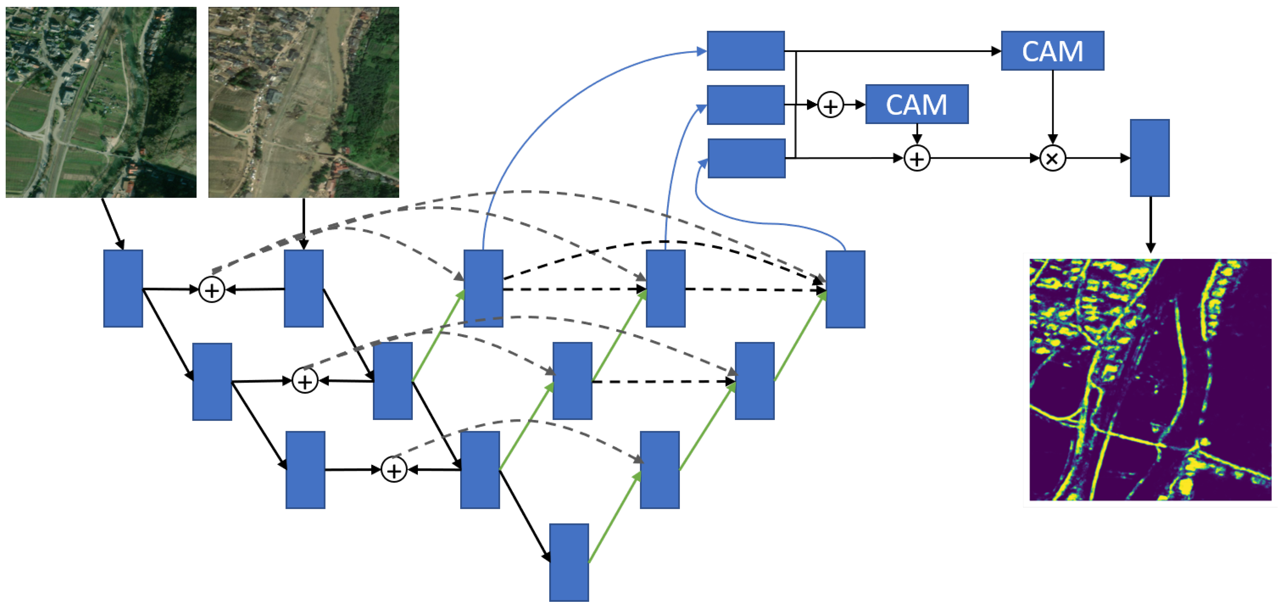
The second TNN-based approach is the SNUNet model from Fang et al. [37]. This model transforms a nested UNet architecture into a TNN by adding another input node and series of down convolutions for the pre-flood image. We did modify the original architecture to reduce the size from four convolutional layers down to only three to get a model that trains faster and works better with our smaller dataset, and our version of the model is shown in Figure 4. Pre- and post-flood image convolutional features are concatenated after each layer (circled plus) then passed via skip connections (dotted gray lines). Each down convolution of the post-flood features has a series of upsamples (green arrows) with the skip connections. Each of the three upsampling series has its own outputs, which are passed through a series of concatenations and CAMs before a final convolutional layer outputs the segmentation mask. For additional details on the model please see Fang et al. [37].
4.1.3. YOLOv8
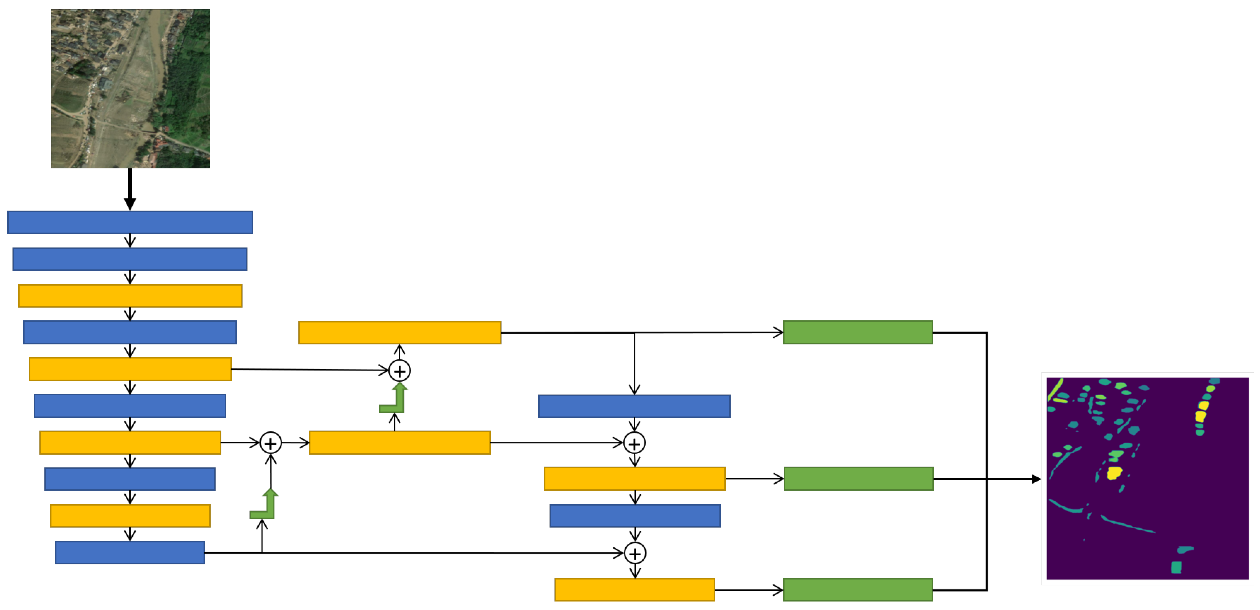
YOLO version 8 (YOLOv8) is a recent version of the YOLO style of object detectors developed by Ultralytics [53]. It is primarily an object detection model but does provide segmentations through a modified head that appends segmentations to detected objects [54]. Figure 5 shows a simplified YOLOv8 architecture based on Terven et al. [54], where a single post-flood image passes through a backbone of convolutional layers. Three different feature layers are pulled and sent through the feature extractor, a series of concatenations, upsamples, and convolutions to extract and mix features at different resolutions. The final set of three extracted features are then sent to three different classification and segmentation heads and combined for the final output. For additional details on YOLOv8 please see Jocher et al. [53] and Terven et al. [54].
We include YOLOv8 because it is a common computer vision algorithm that is easy to use and implement on new datasets. Despite these benefits, YOLOv8 is not the optimal solution for all computer vision tasks, and as we will see in Results (Section 7) it is not the best solution for this segmentation task either. We believe that its inclusion demonstrates the strength of FADS-Fusion with a discount factor to mitigate degradation from a single poor-performing model during fusion. Although this is not optimal, it does explore the benefits of FADS-Fusion.
Figure 4.
The Siamese Nested UNet (SNUNet) model is a TNN built from a modifed nested UNet model, based on the work by Fang et al. [37]. We modified the original architecture to reduce the size from four convolutional layers to three (as shown above) to get a model that trains faster and works better with our smaller dataset. Pre- and post-flood images are input into separate nodes of the model, which are then followed by a series of down convolutions (black arrow to blue box of output feature maps), concatenations (the circled plus), skip connections (gray dashed arrows), and upsamples (green arrows). The backbone outputs are then passed through concatenations and Channel Attention Modules (CAMs) before a final convolutional layer. We sum the segmentation predictions to simplify the figure.
4.2. Dempster–Shafer Theory
Dempster–Shafer Theory is both a theory of evidence and a way to reason probabilistically using the evidence [55], and specifically for FADS-Fusion we use a version of the combination rule from Li et al. [47] to fuse segmentations from the models discussed in the previous section. Besides the benefits of combining evidence to improve performance or measure uncertainty via conflict, Dempster–Shafer Theory also has “characteristics of strong anti-interference, low sensor dependence, and relatively strong fault tolerance”, making it ideal for combining disparate sources for robust results [45].
During inference, we consider a model’s segmentation prediction its belief in the probability of each class per pixel. We ensure that the tensor output matches a standard structure of [B, C, M, N], where B is the batch size, C the number of classes, and M and N are the image width and height. Class probabilities are in the order Building, Flooded Building, Road, Flooded Road, and Empty. We add the Empty class, which is the belief that no objects are in a given pixel, to the ground truth by assigning it a value of 1 for each pixel that is not labeled as another class. This means that each model’s predicted probabilities should sum to 1 (and Empty can be thought of as 1 minus the sum of the four other class beliefs), and we ensure this by using the softmax function [10].
Figure 5.
You Only Look Once version 8 (YOLOv8) takes a single post-flood image and passes it through a backbone of convolutional layers (blue boxes) and C2f (cross-stage partial bottleneck with two convolutions) modules (yellow boxes). Different layers are pulled for the feature extractor portion of the model, upsampled (green arrow), concatenated (the circled plus), passed through more convolutions and C2f modules, and then three extracted features layers are passed into the modified segmentation heads (green boxes) and combined for the final segmentation mask. This figure is based on Figure 17 from Terven et al. [54].
We also apply a discount factor, , which modifies the belief of each model to account for uncertainties in their prediction. The discount factor is the complement of reliability , which can also be considered the degree of trust in the prediction [56]. We use the Mean Average Precision (mAP) performance metric on a validation set as the reliability and modify the predictions with the following equations from [57]:
For the remainder of this article, the beliefs m are modified using Equation (1) and will omit the superscript α. Because there is no prior value of , which is the frame of discernment or list of all outcomes possible [56,57], before this modification the belief in will always match the discount factor ().
We use mAP because it does not depend on a threshold, and therefore the discount factor is not dependent on determining an optimal threshold. Average Precision (AP) does tend to be optimistic in terms of model performance—see Pedregosa et al. [58]—which has also been our experience with it compared to Matthew’s Correlation Coefficient (MCC) or F1. So, mAP will not over-penalize models and dilute the FADS-Fusion results in greater uncertainty because a metric is strict. In the end, we made a judgment call based on these characteristics. Other metrics will work, depending on how you want models to behave, so Intersection over Union (IoU) could focus on particular classes of interest, or Precision or Recall depending on the nature of the problem. Reducing IoU to the Jaccard Index or using MCC would also work.
For a particular outcome A, the fused belief is the summation for all outcomes, k, where the product of outputs from model n, where , show agreement with outcome A divided by the summation for all outcomes where the products of outputs from the models are not in conflict. This form of the fusion is shown in Equation (2):
where A is the fused outcome, k is an outcome (e.g., building or flooded road) from a total of K possibilities, P is the probability of outcome k, and m is the belief, so is the belief from model n that outcome k has occurred in some pixel, which is the same as for model after creating the null class and calculating the softmax above.
For this study, we treat as uncertainty of the actual ground truth, meaning that for a particular model there is an probability the model is uncertain, and the ground truth could be any of the classes. This creates the condition where will have outcome A when using the Dempster–Shafer Fusion Equation (2). We can also consider the uncertainty of the fusion by setting , which is detailed in the next section.
4.3. Uncertainty from Dempster–Shafer
Although Dempster–Shafer can be susceptible to counterintuitive outcomes if the evidence contains high conflict (for example model 1 has a high belief in “building” while model 2 has high belief in “road”) [59], it does provide a way to help make sense of the results, and the discount factor helps to mitigate the impact of high conflict. For FADS-Fusion, we calculate uncertainty via the belief in (Equation (3)), which is the frame of discernment of all possible outcomes, which are supposed to be mutually exclusive [56,57]. Because the prediction cannot be narrowed to a single outcome, we say the model is uncertain.
Because is primarily based on a model’s performance on a validation set, we make the assumption that represents the epistemic uncertainty of the model. However, the influence of aleatoric (or data) uncertainty cannot be entirely removed from , especially because the dataset is small. Our use of cross-validation attempts to limit the impact of aleatoric uncertainty, but it is a limitation of our approach that aleatoric uncertainty cannot entirely be removed from and the uncertainty, U, we calculate in Equation (3).
To see how uncertainty, U, is associated with different class predictions (e.g., is there more or less uncertainty for flooded versus non-flooded objects) we weigh U by the fused belief in each class k as shown in Equation (4):
Details of these implementations can be found in the FADS-Fusion GitHub repository at https://github.com/vtnsi/FADS-Fusion.
5. Evaluating Segmentation Performance
Models are evaluated separately and then fused in pairs using the FADS-Fusion process from the previous section. We use three different metrics for evaluation: Precision (P), Recall (R), mAP, MCC, and IoU. By relying on P, R, mAP (Equation (7)), MCC (Equation (8)) and IoU (Equation (9)), we provide a deeper understanding of model performance than just using any single metric alone. mAP and MCC are calculated to include performance on all the classes, but IoU is at the class level to provide a breakdown of performance on individual classes. The metrics are calculated using functions provided by TorchMetrics [60].
Equation (5) for P, where is true positives and is false positives, calculated with a threshold of 0.5 [60]:
Equation (6) for R, where is true positives and is false negatives, calculated with a threshold of 0.5 [60]:
Equation (7) for mAP averages the class specific precision, where is the average precision for class k and K is the total number of classes [60]:
Equation (8) for the multi-class MCC below is from Pedregosa et al. [58], where k is an outcome from a total of K classes, c is the number of pixels correctly predicted, s is the total number of pixels, is the number of times class k was predicted, and is the number of times class k was correctly predicted:
Finally, Equation (9) for IoU below is from Pedregosa et al. [58], but the values are calculated from the confusion matrix function available in TorchMetrics [60]. Here, are ground truth pixels with class k, are the predicted pixels with class k, are the number of pixels correctly predicted as class k, and is the number of pixels labeled class k by either the model prediction or the ground truth:
Evaluation of prediction uncertainty, U, calculated by the conflict of evidence in the Dempster–Shafer fusion process, is evaluated qualitatively. We plot and compare U at different locations and at different levels of performance to assess the quality of model predictions. By comparing examples of U mapped to the original image at different levels of mAP/MCC, we can see a pattern of prediction/performance quality and the locations where the models struggle to predict. We also create regression scatter plots of the class specific uncertainty, , and U to examine the relationship of uncertainty with model performance.
6. Experimental Setup
All models were trained using a 40 GB partition of a single NVIDIA H100 GPU with PyTorch 2.0.1 [61] and CUDA 11.8. We also used PyTorch Lightning [62] as an additional deep learning framework for training and evaluating the single models and the FADS-Fusion models. Data processing required Geospatial Data Abstraction Library (GDAL) and the Python Package pygdal [63], both of which are version 3.4.1 for our system.
Construction of the seven folds for cross-validation is done by randomly selecting image pairs for the train, validation, and test sets but stratifies them by locations, so each split of each fold has approximately the same ratio of images from Germany and Louisiana as the overall dataset. Data augmentations are not applied onto the training images, which can be seen as a limitation of our work, but the focus was to understand the impact of model fusion only. However, the YOLOv8 package automatically includes augmentations, which were set to the values presented in Table 1 from tuning the model on the pre-flood images.
Table 1.
Augmentation parameters for the YOLOv8 model used in this study. These values were tuned by the Ultralytics tuning function used on pre-flood images.
Each single model required its own set of hyperparameters, but we mostly used the defaults from Hänsch et al. [4] for the SN8 model and from Fang et al. [37] for the SNUNet model. For the YOLOv8 model we used the tune feature offered by Ultralytics [53] to set the hyperparameters on our dataset. Hyperparameters are listed for each model in Table 2 below. The learning rate in Ultralytics is specified by the starting learning rate (lr0) and the ratio of lr0 that defines the final learning rate (lrf), so the final learning rate is , and we used the default scheduler in Ultralytics for training, so step size and gamma are not set.
Table 2.
Hyperparameters for training the SN8, SNUNet, and YOLO models used in this study. Note that the YOLO hyperparameters use the default Ultralytics scheduler with a starting learning rate of and that is the ratio of the learning rate will reach at the end of training.
7. Results
7.1. Cross-Validation Fold and Image-Level Results
The results for each model across all the seven-fold test sets are aggregated together for a fold-level comparison of each metric. Figure 6 shows mAP as a candlewick plot, with the mean value across all folds at the level fo the bar and a 95% confidence interval as the vertical line centered at the top of the bar. We can see that the baseline SpaceNet 8 model (SN8) is the best performing single model (i.e., not fused) with a 0.672 mAP and 0.642 MCC. The YOLO model does poorly, much more than expected for such a popular object detection model, but they can struggle with small objects in the image and that is likely what happened here [64]. The SNUNet model does moderate with a 0.537 mAP, 0.550 MCC, and a larger confidence interval. Fusing these models together, we can see that the mean performance of the SN8 and SNUNet models fused via FADS-Fusion (SN8 + SNUNet) marginally improve performance: the mAP increases to 0.685 (1.93% improvement) and MCC to 0.654 (1.87% improvement), demonstrating a small benefit of decision fusion of these models.
Figure 6.
Mean Average Precision (mAP) results for each model across the seven cross-validation folds. SN8, SNUNet, and YOLO are the individual models and SN8 + SNUNet and SN8 + YOLO are combined using the FADS-Fusion process. Fusing model outputs improves performance above the baseline SN8 model, although that improvement is marginal.
Even with under-performing single models, like YOLO, there can be some improvement from Dempster–Shafer fusion because we include the discount factor to limit the influence of the worse model. We still see some benefit with fusing SN8 and YOLO (SN8 + YOLO): mAP increases to 0.684 (1.79% improvement), but MCC drops to 0.641 (0.16% decrease) compared to the SN8 model alone.
Across all metrics we used, shown in Table 3, we see that SN8 + SNUNet performs the best in all metrics except Recall (−15.0%), where SN8 performs best. FADS-Fusion demonstrates a fairly robust improvement across all but one metric, even though improvements are small. We see the largest improvements for flooded and non-flooded road IoUs (+5.50% and +2.33% respectively) and Precision (+12.3%) of the SN8 + SNUNet model over the SN8 baseline. Meaning the Dempster–Shafer fusion with a discount factor process makes a marked improvement for road extraction, especially for flooded roads, and in reducing false positives (given the increased Precision) but increasing false negatives (given the decrease in Recall). We performed a paired t-test comparing each metric of the SN8 baseline and SN8 + SNUNet fusion models, with results presented in Table 4. The only differences which are statistically significant are the +12.3% increase for Precision and the −15.0% decrease in Recall. In terms of segmentation performance, this means the FADS-Fusion process reduces false positives, focusing on areas where the two models agree more, but this can increase false negatives. While the FADS-Fusion process for the SN8 + SNUNet model appears to increase performance across the other metics (mAP, MCC, IoUs), these are modest and not statistically significant. Performance could vary on different datasets, and therefore we acknowledge that these results are more exploratory than definitive.
Table 3.
Tabulated results for each model across the seven cross-validation folds. This includes the mAP values that match the bars in Figure 6 as well as the rest of the metrics used for evaluation. The best performing value per column is in bold. The SN8 + SNUNet model performs the best for each metric except Recall.
Table 4.
Tabulated t-test results comparing the SN8 + SNUNet fusion model to the SN8 baseline based on image level performance for each metric. The only statistically significant differences are between Precision and Recall (Statistic and p-Value in bold), with the SN8 + SNUNet having greater Precision performance over the baseline but lesser Recall.
We also analyze metrics at the image level, meaning we record and pool the metrics calculated per image. We also split these image level results by the presence or absence of flooded objects (buildings or roads) to see how performance changes. Because, as noted in Section 3, the majority of image pairs have no flooded objects in the post-disaster image, we expect to see a difference in performance in this split. Figure 7 shows the mAP of each model split by images without flooded objects (blue) and images with at least one flooded object (orange). There is a noticeable drop in mAP for each model when there is flooding in the image, which is not ideal for a flood detection model but indicates that the lack of images with flooded objects in the dataset is detrimental to performance in that domain.
Figure 7.
Mean Average Precision (mAP) results for each model based on individual image results. Here, we have also split the images based on the presence of any flooded buildings or roads (orange) or no flooded objects (blue). Performance trends are similar to those for the fold-level results in Figure 6, but we see that all models perform worse with the flooded images.
Overall, the models compare to each other similarly to how they compared with the fold-level results in Figure 6. We do see that the SN8 + SNUNet FADS-Fusion results have improved for images without flooded objects over the SN8 model; from an mAP of 0.690 for SN8 to 0.701 for SN8 + SNUNet (+1.59%) and an MCC of 0.597 to 0.604 (+1.17%). For images with flooded objects the fusion improves mAP from 0.585 for SN8 to 0.595 for SN8 + SNUNet (+1.71%) and an MCC of 0.524 to 0.526 (+0.38%). The Dempster–Shafer fusion results for SN8 + SNUNet have better performance across all the metrics in Table 5 and Table 6, except for Recall, demonstrating the improvement is robust, albeit small. We also see a small improvement for the SN8 + YOLO FADS-Fusion results, but just for mAP and Precision, as all other metrics have decreased compared to SN8 alone in either Table 5 or Table 6.
Table 5.
Tabulated results for each model aggregating results for images with flooding present. This includes the mAP values that match the bars in Figure 7 as well as the rest of the metrics used for evaluation. The best performing value per column is in bold. The SN8 + SNUNet model performs the best for each metric except flooded-building IoU and Recall.
Table 6.
Tabulated results for each model aggregating results for images with no flooding present. This includes the mAP values that match the bars in Figure 7 as well as the rest of the metrics used for evaluation. The best performing value per column is in bold. The SN8 + SNUNet model performs the best for each metric except Recall.
7.2. Fusion Uncertainty Quantification
Dempster–Shafer fusion provides a method for quantifying uncertainty between the model outputs being fused together using evidence conflict, which was detailed in Section 4.3. Because uncertainty is calculated per pixel we can map the uncertainty onto the image to gain insights about the models’ predictions. In Figure 8 there are nine examples of uncertainty mapped back onto images with varying levels of total uncertainty and mAP performance for the SN8 + SNUNet FADS-Fusion model. Values for mAP, MCC, and mean uncertainty for these images are in Table 7.
Figure 8.
Nine examples of uncertainty from the SN8 + SNUNet fusion using the FADS-Fusion process are mapped back onto images with varying levels of total uncertainty (x-axis) and mAP performance (y-axis). Images moving from left to right have low, mid, and high uncertainty and images from bottom to top have low, mid, and high mAP performance. Values for mAP, MCC, and mean uncertainty for these images are listed in Table 7.
Table 7.
mAP, MCC, and mean uncertainty values for the images shown in Figure 8, including a label of low, mid, or high mAP and uncertainty and a note on why the mAP value is in the tier it is in.
The columns on the left have low uncertainty and tend to have fewer objects. As the column moves right the uncertainty increases and so does the number of objects in the image. The total amount of calculated uncertainty corresponds with the total number of objects in the image rather than how well the fusion process performed with that image. Fused outputs where uncertainty tends to outline the objects (the right two columns of the top row) correspond with better performance; we see clear boundaries for buildings and roads, meaning the fused models have agreement on where the objects are but conflict on exact boundaries. We also see several buildings and some roads highlighted either in partial or full, indicating that one model struggled while the other model did not.
Images where roads or buildings have uncertainty filling the inner regions, however, have poorer performance. These are areas where a human user would need to double check to confirm the predictions of the model. Based on the visual quality of these uncertainty map images we can assess how confident we can be about the performance of the fusion model. This provides users/operators a way to easily and visually assess what is going on and identify where they need to look to make a manual assessment.
Higher uncertainty correlates more with object count in the image than with actual performance of the models. Figure 9 shows the correlation between object count and uncertainty; however, both a high uncertainty and a high object count do not indicate that FADS-Fusion will perform worse on a sample image pair. In Figure 10, both images have a large number of objects. The image on the right of Figure 10, however, has a higher mean uncertainty, 0.1791, but the SN8 + SNUNet fusion model performs better on it, with an mAP of 0.8834 and an MCC of 0.7549. The image on the left has a mean uncertainty of 0.1769, while its performance metrics are an mAP of 0.4845 and an MCC of 0.5675. Although both images have a high object count we can see that the image on the left has many object interiors filled with greater uncertainty values while the image on the right mostly has uncertainty at the edges of objects (with some exceptions).
Figure 9.
Scatter plot with linear regression to show the correlation between object count in an image and the uncertainty from FADS-Fusion.
Figure 10.
Comparison of two fused images with high uncertainty. The uncertainty from the SN8 + SNUNet fusion using the FADS-Fusion process are mapped back onto images. On the left, mean uncertainty is 0.1769 and we can see many object interiors filled with greater uncertainty values. On the right, mean uncertainty is 0.1791 and we can see most of the mapped uncertainty at the edges of objects. The fused results for the image on the right have a greater mAP and MCC than the one on the left. Higher uncertainty does not mean worse performance, but a visual assessment of the uncertainty can provide insight on performance.
To try and better understand the relationship between uncertainty and performance, Figure 11 shows a scatter plot of class-weighted uncertainty, (Equation (4)), overlaid with a regression line compared to MCC. Each subplot shows the mean uncertainty weighted by each individual class from all the pixels within an image, and we can see MCC tends to increase with non-flooded building and road uncertainty while it decreases with flooded building and road uncertainty. There are two mechanisms going on here: (1) more objects in the image means mistakes are less critical to overall performance, so higher uncertainty becomes associated with improved performance in non-flooded images, and (2) the models have difficulty with flooded images because they are underrepresented in the dataset, so higher uncertainty in flooded images is associated with reduced performance because there are more flooded objects to identify and one or both models are struggling with segmenting them. Knowing this and the number of predicted flooded objects and looking at the uncertainty map can provide a more complete evaluation of the model performance.
Figure 11.
Scatter plots of class-weighted uncertainty, (Equation (4)), on the x-axis compared with MCC values per image on the y-axis, and regression line. Uncertainty has mild positive correlation for non-flooded buildings and roads, and mild negative correlation for flooded buildings and roads.
Finally, to better understand the relationship between uncertainties (total and class-weighted), presence of flooding, and other potential factors impacting MCC performance, we performed an Analysis of Variance (ANOVA) using an Ordinary Least Squares (OLS) linear regression model using the Statsmodels Python package [65]. We included second and third order interactions between these factors, then created a reduced-order model based on the main factors and significant interactions. This model fit the data with an adjusted value of 0.347 and a p-value of 6.92 .
The coefficients of this reduced order model are presented in Table 8. A table of ANOVA results for the statistically significant variables of the reduced order model are presented in Table 9. The total image uncertainty is significant with a negative effect (−59.08) on performance, meaning a 0.001 increase in uncertainty will result in a −0.05908 drop in MCC. This decrease is slight, and total uncertainty interacts with building and road-weighted uncertainty, as well as location. It is also important to note that while the interactions of uncertainties have high coefficients in the OLS model, because the values of uncertainty are so small the interactions will also be small.
Table 8.
Coefficients and statistical test results for an Ordinary Least Squares (OLS) linear regression model using the Statsmodels Python package [65]. This model fits uncertainties, object count, location, presence of flooding, and fold, along with second and third order interactions between these variables, with the MCC performance of the SN8 + SNUNet fusion model.
Table 9.
Tabulated ANOVA results for the variables and interactions of variables that are statistically significant from from the Ordinary Least Squares (OLS) linear regression model using the Statsmodels Python package [65] to fit uncertainties, object count, location, presence of flooding, and fold with the MCC performance of the SN8 + SNUNet fusion model. These results are derived from the model summarized in Table 8.
Despite the correlation between uncertainty and object count, the latter does not have a statistically significant impact on performance nor does its interactions with the other variables. It is also surprising that flood presence is not statistically significant, as we saw a drop in performance for all models between images with Flooded infrastructure compared to images without (see Figure 7). Other factors that are significant include fold and location. This means that performance on data in Louisiana-East is greater than Germany, which coincides with the amount of data from each in the datasets (599 images from Louisiana and only 202 from Germany). The significance of the fold on performance indicates that despite stratifying the folds by location, there are differences amongst them. This could mean that there is variation in the data that is hard to balance by splitting into folds, and future work with this dataset could require greater care in designing splits.
7.3. Computational Costs
During inference, the additional computational costs for the FADS-Fusion (loading a second model, combining outputs, and calculating uncertainty) are small relative to the cost of loading and processing the data. The SN8 Baseline uses about 10.6 GB of GPU memory to load the model and perform the inference on the entire test set. The SNUNet model uses about 15 GB of GPU memory for the same task. When fusing the models, however, there is only the addition of one model and not the data, so the total GPU memory is 16.1 GB to load both models and perform the inference and calculate uncertainty, approximately a 1 GB increase in GPU memory.
There is a similar but less pronounced difference with the SN8 and YOLO model fusion. The YOLOv8 model has more variability in the amount of GPU memory required, using an average of 13.9 GB of GPU across the seven folds, but this ranged from 11.0 GB to 19.0 GB. Fusing SN8 + YOLO required an average of 14.2 GB, with a range of 12.2 GB to 17.7 GB. It is unclear why there is so much variability, but we can conservatively estimate a 1 GB increase in GPU memory.
Memory was recorded using the nvidia-smi command line utility during model evaluations. The difference in time was negligible, as all models and model fusion took a minute or less to run inference on the whole test set.
8. Discussion
8.1. Dempster–Shafer for Improved Infrastructure Segmentation
The baseline SN8 model from Hänsch et al. [4] was the best performing individual model both at the cross-validation fold level and at the image level. When using FADS-Fusion to fuse the outputs from this model with the SNUNet (SN8 + SNUNet), the mAP performance increases by +1.93% at the fold level, +1.59% at the non-flooded image level, and +1.71% at the flooded image level. Although these improvements are modest, we show that the FADS-Fusion has the potential to improve performance over the single models for segmenting infrastructure in pre- and post-flood image; however, we acknowledge that these results are more exploratory than definitive. There are statistically significant differences for the SN8 + SNUNet model of +12.3% for Precision and −15.0% in Recall compared to the SN8 Baseline. This indicates that FADS-Fusion can reduce false positives by focusing on areas where the two models agree more, but this can increase false negatives. The dataset for this task was small, with 801 images that had to be divided between training, validation, and testing, meaning approximately 570 images for training. Also, the majority of post-disaster images did not have any flooded infrastructure in them. Given these facts, the number of samples for the models to learn what flooded infrastructure looks like is small. Therefore, the marginal increases of FADS-Fusion on the suite of metrics is not unexpected and demonstrates its applicability to this task.
While our approach is another in a long line of deep learning algorithms for disaster management, there is less research focused on flooding and damage detection [19]. Our work is methodologically novel in that the application of Dempster–Shafer for multi-model fusion and uncertainty quantification on a flood dataset for segmenting both buildings and roads, and whether they are flooded or not, has not been done in the existing literature. It also addresses one of the open challenges for “improving the model performance in the inference stage... without the need to retrain a deep learning model” [10]. Most previous work focused on single-model feature-level fusion [6,7,17,34,38,39], which offered improvements but required custom model architecture for their particular combination of data sources. And road segmentation work was primarily done in isolation of buildings, as road detection is a challenging problem in and of itself [9,42]. The closest previous works to our study were Ghasemian Sorboni et al. [35] and Yadav et al. [36], but they both focused on using pre- and post-flood images to label flood waters only and not discern flooded from non-flooded infrastructure. Although our SNUNet model is based on the model from Fang et al. [37], those authors did not apply their model to flood detection. Our approach with Dempster–Shafer applies to high resolution imagery and generalizes to tasks that already have any existing pre-trained model, so unlike the majority of previous works, a custom architecture is not required for our approach to be applied to new tasks. It does require, however, that the outputs from models are standardized to fuse them properly, but this can be a post-processing step.
While FADS-Fusion offers effective segmentation of flooded and non-flooded buildings and roads in our study, the improvement over the single SN8 model was modest at best. Most other works saw greater improvements in IoU metrics for building or road segmentation [6,7,17]. And, while not a direct comparison because of the differences in data, our FADS-Fusion approach increased Precision at the cost of Recall and the work by Wang et al. [10], with test-time augmentations and Dempster–Shafer Fusion, also increased Precision at the cost of Recall for road segmentation. Our study builds on these previous works by turning Dempster–Shafer to multi-model fusion, which can make use of pretrained models with different advantages and disadvantages depending on the context of the flood, location, and available data modalities. While multi-model fusion is known to improve performance and reduce the uncertainty over a single model [10] and can help create more robust and transferrable models [11,12,13,14]; our study found a more modest improvement in performance metrics of the multi-model fusion via FADS-Fusion, but a statistically significant increase in Precision at a cost of Recall.
8.2. Dempster–Shafer for Uncertainty Quantification
For uncertainty quantification, we used conflict of evidence between two models and applied a discount factor to belief (model prediction) with the the Dempster–Shafer theory combination rule (Section 4.2). This not only allowed us to assess disagreement between the fused models but also weigh uncertainty by class and localize it in the original image. While total uncertainty in the images correlated with a drop in performance (see Table 8), this relationship also depends on the values for class-weighted uncertainty for building and road as well as the location. This means that uncertainty can be used as a quantitative indicator of performance but additional criteria are needed. Future work could extend the FADS-Fusion UQ by building an additional model to predict performance, or relative change, based on uncertainty and image metadata.
The other advantage of FADS-Fusion uncertainty quantification, localizing uncertainty in the image, gives the user the ability to visually assess the quality of the fusion (i.e., the model performance) and see where the models conflict (i.e., where is the area a human needs to correct or inspect). One of the needs highlighted in several previous studies is explainability and interpretability for flood-related AI [5,19,48]. Most of the approaches we found relied on additional models to calculate uncertainty [47] or needed to modify the main deep learning model to use uncertainty [18,49]. Our approach, using Dempster–Shafer for model fusion, directly addresses this need in the literature via both qualitative and quantitative means. More research is required; however, FADS-Fusion offers a starting point to address the need for explainability in post-flood disaster response modeling. It also demonstrates that multi-model fusion is one path towards uncertainty quantification and explainability for post-flood damage assessment, which has not been done, as far as we know, in the literature before.
Uncertainty quantification can be performed with only a single model, but this requires: (1) test-time augmentations, i.e., augmenting a single image a few dozen times and calculating uncertainty based on how the model outputs change [10]; or (2) training a model with dropout and running inference with the dropout on, which produces more stochastic outputs and with a few dozen iterations the uncertainty can be calculated [15]. The disadvantage of these methods is the number of iterations to calculate uncertainty (10–50 times to get enough sample outputs), and the dropout method requires the model to be trained with dropout (which takes more training time). With multi-model fusion, we can reduce the inference time by only using two or a handful of models. A user could select two models trained in the same or similar regions to improve performance and not degrade inference time. On the other hand, if the region is different from data used to train the available models, a user could select several models for fusion and effectively ensemble the poor decisions out. The discount factor can be set based on a pretrained model’s past performance, or the user can set it based on their knowledge of how the model would apply in a new situation. In short, it offers greater flexibility. On the other hand, our method does require greater computational resources at inference to run multiple models at once, though this could be solved via batching and saving intermediate outputs from single models.
8.3. Limitations
Dempster–Shafer fusion can have counterintuitive results when models are in high conflict [66]. Applying a discount factor helps mitigate this, which is why the fused results of SN8 + YOLO work but essentially match the performance of SN8 for most metrics except mAP, Precision, and Recall (Table 3). The discount factor, however, would not help in situations where the reliabilities of two models are similar and their predictions are in high conflict. Calculating and mapping uncertainty can help identify where this issue could be occurring, but it would not correct the issue, it would just highlight the area for a human user to inspect and correct later. In either case, we feel that using both the fused results and the uncertainty map with models that have similar behavior is the best way to minimize this issue.
The other limitation we faced was the size of the dataset—801 images divided amongst training, validation, and testing, leaving approximately 570 images for training. Also, the majority of post-disaster images did not have any flooded infrastructure in them and as a result we see the model under-perform in images that have flooding. This is, however, a typical small and imbalanced data problem. The small dataset size does raise concerns for statistical robustness and overfitting. To address this we employed cross-validation to average out the randomness of each fold and limited the training epochs to around 50–60 (see Section 6). Despite these measures, the small dataset is an inherent limitation on our study and its generalizability.
Given the task to label both flooded buildings and roads, we did not find any datasets that contained the same combination of flooded and non-flooded labels for buildings and roads. Most focused on one type of infrastructure or identifying generally flooded areas. More data would improve the performance of the base models even more, and therefore make the Dempster–Shafer fused results better and help address the issues with the conflict mentioned above.
9. Conclusions
We developed FADS-Fusion, a tool which uses Dempster–Shafer’s Combination Rule, with a discount factor, for segmentation model fusion and uncertainty quantification to assess flood damage in pre- and post-flood satellite imagery. We fine-tuned the SpaceNet 8 Baseline TNN (SN8), a modified SNUNet TNN, and YOLOv8 models on the SpaceNet 8 challenge dataset for pixel-wise segmentation of non-flooded buildings, non-flooded roads, flooded buildings, and flooded roads. All results were post-processed to match structure and create a null class, and then we fused results from two models (SN8 + YOLO and SN8 + SNUNet).
We found that the UNet-based architectures (SN8 and SNUNet) outperformed the YOLOv8 architecture for segmentation. Using FADS-Fusion with SN8 + SNUNet gave a modest improvement in mAP at the fold-level (+1.93%) and image-level (+1.59% for non-flooded and +1.71% for flooded), and we acknowledge that these results are more exploratory than definitive results. However, there is a +12.3% increase for Precision and a −15.0% decrease in Recall, which are statistically significant compared to the baseline. For the image-level results, we split the metrics by the presence or absence of flooded objects and showed the difficulty with flooded images in the dataset, as not every pre- and post-flood image pair had flooded objects. Overall, the models performed worse on the images with flooding compared to non-flooded image pairs, but this can be addressed in future efforts by using a larger dataset.
We used the conflict of evidence and discount factors based on each model’s mAP performance on a validation set with FADS-Fusion to quantify the uncertainty between the two models, then weighted this by class probability for each pixel. While total image uncertainty correlates with a drop in performance (see Table 8), this relationship also depends on the values for class-weighted uncertainty for building and road as well as the location. This means that uncertainty can be used as a quantitative indicator of performance but additional criteria are needed. Quantifying uncertainty also provides additional context by mapping it onto the original image to show quality of segmentation, as well as the areas a human user should double check. Conflict in Dempster–Shafer does come with the caveat that a greater difference in model predictions can lead to counter-intuitive results. Even with this caveat, we demonstrated that quantifying uncertainty provides explainability in post-flood damage assessment for better context and decision-making, something that is still in need of more research for the use of AI in disaster management.
Decision-level model fusion makes better use of existing deep learning models which could be trained on data from particular regions or have advantages/disadvantages for certain scenarios. For example, some models might be better at identifying roads but struggle with flood waters, while another might be better at detecting buildings. We demonstrated that the FADS-Fusion tool improves performance and provides UQ for post-flood damage assessment, but it could be expanded to other segmentation tasks related to post-disaster management or change detection. Future work could extend the FADS-Fusion UQ by building an additional model to predict performance, or relative change, based on uncertainties and image metadata. It could also focus on expanding FADS-Fusion to other, larger, datasets to address limitations caused by the dataset size; or explore different metrics to use for the discount factor or to try optimizing a value.
Author Contributions
Conceptualization, D.S. and C.S.; methodology, D.S.; software, D.S.; formal analysis, D.S.; data curation, D.S. and C.S.; writing—original draft preparation, D.S.; writing—review and editing, D.S. and C.S. All authors have read and agreed to the published version of the manuscript.
Funding
This research received no external funding.
Data Availability Statement
The original data presented in the study are openly available from SpaceNet as a public AWS dataset at https://spacenet.ai/sn8-challenge/ (accessed on 27 March 2024) or https://registry.opendata.aws/spacenet (accessed on 27 March 2024). Code for the FADS-Fusion tool is available on GitHub at https://github.com/vtnsi/FADS-Fusion.
Acknowledgments
We would like to thank the Virginia Tech National Security Institute and the Virginia Tech Center for Geospatial Information Technology for their guidance and support of this work. We would also like to thank the anonymized reviewers for their constructive feedback and help to improve this article.
Conflicts of Interest
The authors declare no conflicts of interest.
Abbreviations
The following abbreviations are used in this manuscript:
| AI | Artificial Intelligence |
| ANN | Artificial Neural Network |
| ANOVA | Analysis of Variance |
| AP | Average Precision |
| CAM | Channel Attention Module |
| CDF | Cumulative Distribution Function |
| CNN | Convolutional Neural Network |
| CRF | Conditional Random Field |
| EO | Electro-Optical |
| FADS-Fusion | Flood Assessment using Dempster–Shafer Fusion |
| FIMA | Federal Insurance and Mitigation Administration |
| FN | False Negative |
| FP | False Positive |
| GAN | Generative Adversarial Network |
| GDAL | Geospatial Data Abstraction Library |
| GPU | Graphics Processing Unit |
| IoU | Intersection Over Union |
| LCLU | Land-Cover and Land-Use |
| lr | Learning Rate |
| mAP | Mean Average Precision |
| MCC | Matthew’s Correlation Coefficient |
| ML | Machine Learning |
| NFIP | National Flood Insurance Program |
| OBCD | Object-Based Change Detection |
| OLS | Ordinary Least Squares |
| P | Precision |
| PBCD | Pixel-Based Change Detection |
| R | Recall |
| RCNN | Region Convolutional Neural Network |
| RGB | Red Green Blue |
| SAR | Synthetic Aperture Radar |
| SN8 | SpaceNet 8 (Baseline) |
| SNUNet | Siamese Nested UNet |
| SVM | Support Vector Machine |
| TN | True Negative |
| TNN | Twin Neural Network |
| TP | True Positive |
| UAV | Unmanned Aerial Vehicle |
| UQ | Uncertainty Quantification |
| VHR | Very High Resolution |
| YOLO | You Only Look Once |
References
- Munawar, H.S. Flood disaster management: Risks, technologies, and future directions. Mach. Vis. Insp. Syst. Image Process. Concepts Methodol. Appl. 2020, 1, 115–146. [Google Scholar]
- Union of Concerned Scientists. Climate Change, Extreme Precipitation, and Flooding: The Latest Science; Union of Concerned Scientists: Cambridge, MA, USA, 2018. [Google Scholar]
- Eekhout, J.P.; Hunink, J.E.; Terink, W.; de Vente, J. Why increased extreme precipitation under climate change negatively affects water security. Hydrol. Earth Syst. Sci. 2018, 22, 5935–5946. [Google Scholar] [CrossRef] [Scilit]
- Hänsch, R.; Arndt, J.; Lunga, D.; Gibb, M.; Pedelose, T.; Boedihardjo, A.; Petrie, D.; Bacastow, T.M. Spacenet 8-the detection of flooded roads and buildings. In Proceedings of the IEEE/CVF Conference on Computer Vision and Pattern Recognition, New Orleans, LA, USA, 19–20 June 2022; pp. 1472–1480. [Google Scholar]
- Sun, W.; Bocchini, P.; Davison, B.D. Applications of artificial intelligence for disaster management. Nat. Hazards 2020, 103, 2631–2689. [Google Scholar] [CrossRef] [Scilit]
- Drakonakis, G.I.; Tsagkatakis, G.; Fotiadou, K.; Tsakalides, P. Ombrianet—supervised flood mapping via convolutional neural networks using multitemporal sentinel-1 and sentinel-2 data fusion. IEEE J. Sel. Top. Appl. Earth Obs. Remote Sens. 2022, 15, 2341–2356. [Google Scholar] [CrossRef] [Scilit]
- Sanderson, J.; Mao, H.; Abdullah, M.A.; Al-Nima, R.R.O.; Woo, W.L. Optimal Fusion of Multispectral Optical and SAR Images for Flood Inundation Mapping through Explainable Deep Learning. Information 2023, 14, 660. [Google Scholar] [CrossRef] [Scilit]
- Sghaier, M.O.; Lepage, R. Change detection using multiscale segmentation and Kullback-Leibler divergence: Application on road damage extraction. In Proceedings of the 2015 8th International Workshop on the Analysis of Multitemporal Remote Sensing Images (Multi-Temp), Annecy, France, 22–24 July 2015; pp. 1–4. [Google Scholar]
- Weixing, W.; Limin, L.; Zhen, Z. Road extraction in vague images on gray scale consistency and improved MSR and DS evidence. Multimed. Tools Appl. 2022, 81, 43657–43678. [Google Scholar] [CrossRef] [Scilit]
- Wang, Z.; Wang, Z.; Zeng, H.; You, S.; Zhang, Q. DeepDSFusion: A General Multiscale Decision Fusion Method for Segmentation Tasks on High-Resolution Imagery with Deep Learning. IEEE Geosci. Remote Sens. Lett. 2023, 20, 6007505. [Google Scholar] [CrossRef] [Scilit]
- Krometis, J.A.; Sobien, D.; Kyer, A.; Kauffman, J.A. Sensor Data Fusion for Adversarial Patch Attack Mitigation. In Proceedings of the AIAA SCITECH 2026 Forum, Orlando, FL, USA, 12–16 January 2026; p. 0431. [Google Scholar]
- Peterson, K.T.; Sagan, V.; Sidike, P.; Hasenmueller, E.A.; Sloan, J.J.; Knouft, J.H. Machine learning-based ensemble prediction of water-quality variables using feature-level and decision-level fusion with proximal remote sensing. Photogramm. Eng. Remote Sens. 2019, 85, 269–280. [Google Scholar] [CrossRef] [Scilit]
- Feilhauer, H.; Asner, G.P.; Martin, R.E. Multi-method ensemble selection of spectral bands related to leaf biochemistry. Remote Sens. Environ. 2015, 164, 57–65. [Google Scholar] [CrossRef] [Scilit]
- Ghulam, A.; Kusky, T.M.; Teyip, T.; Qin, Q. Sub-canopy soil moisture modeling in n-dimensional spectral feature space. Photogramm. Eng. Remote Sens. 2011, 77, 149–156. [Google Scholar] [CrossRef] [Scilit]
- Costa, M.; Sobien, D.; Garg, R.; Cheung, W.; Krometis, J.; Kauffman, J.A. Uncertainty quantification in data fusion classifier for ship-wake detection. Remote Sens. 2024, 16, 4669. [Google Scholar] [CrossRef] [Scilit]
- Sovacool, B.K.; Axsen, J.; Sorrell, S. Promoting novelty, rigor, and style in energy social science: Towards codes of practice for appropriate methods and research design. Energy Res. Soc. Sci. 2018, 45, 12–42. [Google Scholar] [CrossRef] [Scilit]
- Rudner, T.G.; Rußwurm, M.; Fil, J.; Pelich, R.; Bischke, B.; Kopačková, V.; Biliński, P. Multi3net: Segmenting flooded buildings via fusion of multiresolution, multisensor, and multitemporal satellite imagery. In Proceedings of the AAAI Conference on Artificial Intelligence, Honolulu, HI, USA, 27 January–1 February 2019; Volume 33, pp. 702–709. [Google Scholar]
- Cheng, C.S.; Behzadan, A.H.; Noshadravan, A. Uncertainty-aware convolutional neural network for explainable artificial intelligence-assisted disaster damage assessment. Struct. Control Health Monit. 2022, 29, e3019. [Google Scholar] [CrossRef] [Scilit]
- Linardos, V.; Drakaki, M.; Tzionas, P.; Karnavas, Y.L. Machine learning in disaster management: Recent developments in methods and applications. Mach. Learn. Knowl. Extr. 2022, 4, 446–473. [Google Scholar] [CrossRef] [Scilit]
- Rizk, Y.; Jomaa, H.S.; Awad, M.; Castillo, C. A computationally efficient multi-modal classification approach of disaster-related Twitter images. In Proceedings of the 34th ACM/SIGAPP Symposium on Applied Computing, Limassol, Cyprus, 8–12 April 2019; pp. 2050–2059. [Google Scholar]
- Cervone, G.; Sava, E.; Huang, Q.; Schnebele, E.; Harrison, J.; Waters, N. Using Twitter for tasking remote-sensing data collection and damage assessment: 2013 Boulder flood case study. Int. J. Remote Sens. 2016, 37, 100–124. [Google Scholar] [CrossRef] [Scilit]
- Nguyen, D.T.; Ofli, F.; Imran, M.; Mitra, P. Damage assessment from social media imagery data during disasters. In Proceedings of the 2017 IEEE/ACM International Conference on Advances in Social Networks Analysis and Mining, Sydney, Australia, 31 July–3 August 2017; pp. 569–576. [Google Scholar]
- Akshya, J.; Priyadarsini, P. A hybrid machine learning approach for classifying aerial images of flood-hit areas. In Proceedings of the 2019 International Conference on Computational Intelligence in Data Science (ICCIDS), Chennai, India, 21–23 February 2019; pp. 1–5. [Google Scholar]
- Yang, L.; Cervone, G. Analysis of remote sensing imagery for disaster assessment using deep learning: A case study of flooding event. Soft Comput. 2019, 23, 13393–13408. [Google Scholar] [CrossRef] [Scilit]
- van Aardt, J.A.; McKeown, D.; Faulring, J.; Raqueño, N.; Casterline, M.; Renschler, C.; Eguchi, R.; Messinger, D.; Krzaczek, R.; Cavillia, S.; et al. Geospatial disaster response during the Haiti earthquake: A case study spanning airborne deployment, data collection, transfer, processing, and dissemination. Photogramm. Eng. Remote Sens. 2011, 77, 943–952. [Google Scholar] [CrossRef] [Scilit]
- Bevington, J.S.; Eguchi, R.T.; Gill, S.; Ghosh, S.; Huyck, C.K. A comprehensive analysis of building damage in the 2010 Haiti earthquake using high-resolution imagery and crowdsourcing. In Time-Sensitive Remote Sensing; Springer: New York, NY, USA, 2015; pp. 131–145. [Google Scholar]
- Hernández, D.; Cecilia, J.M.; Cano, J.C.; Calafate, C.T. Flood detection using real-time image segmentation from unmanned aerial vehicles on edge-computing platform. Remote Sens. 2022, 14, 223. [Google Scholar] [CrossRef] [Scilit]
- Ichim, L.; Popescu, D. Segmentation of vegetation and flood from aerial images based on decision fusion of neural networks. Remote Sens. 2020, 12, 2490. [Google Scholar] [CrossRef] [Scilit]
- Munawar, H.S.; Ullah, F.; Qayyum, S.; Heravi, A. Application of deep learning on uav-based aerial images for flood detection. Smart Cities 2021, 4, 1220–1242. [Google Scholar] [CrossRef] [Scilit]
- Rahnemoonfar, M.; Chowdhury, T.; Sarkar, A.; Varshney, D.; Yari, M.; Murphy, R.R. Floodnet: A high resolution aerial imagery dataset for post flood scene understanding. IEEE Access 2021, 9, 89644–89654. [Google Scholar] [CrossRef] [Scilit]
- Munawar, H.S.; Hammad, A.W.; Waller, S.T. A review on flood management technologies related to image processing and machine learning. Autom. Constr. 2021, 132, 103916. [Google Scholar] [CrossRef] [Scilit]
- Bentivoglio, R.; Isufi, E.; Jonkman, S.N.; Taormina, R. Deep learning methods for flood mapping: A review of existing applications and future research directions. Hydrol. Earth Syst. Sci. Discuss. 2022, 26, 4345–4378. [Google Scholar] [CrossRef] [Scilit]
- Katiyar, V.; Tamkuan, N.; Nagai, M. Near-real-time flood mapping using off-the-shelf models with SAR imagery and deep learning. Remote Sens. 2021, 13, 2334. [Google Scholar] [CrossRef] [Scilit]
- Wu, H.; Song, H.; Huang, J.; Zhong, H.; Zhan, R.; Teng, X.; Qiu, Z.; He, M.; Cao, J. Flood detection in dual-polarization SAR images based on multi-scale deeplab model. Remote Sens. 2022, 14, 5181. [Google Scholar] [CrossRef] [Scilit]
- Ghasemian Sorboni, N.; Wang, J.; Najafi, M.R. Urban flood mapping using Sentinel-1 and RADARSAT Constellation Mission image and convolutional Siamese network. Nat. Hazards 2024, 120, 5711–5742. [Google Scholar] [CrossRef] [Scilit]
- Yadav, R.; Nascetti, A.; Ban, Y. Attentive dual stream siamese u-net for flood detection on multi-temporal sentinel-1 data. In Proceedings of the IGARSS 2022-2022 IEEE International Geoscience and Remote Sensing Symposium, Kuala Lumpur, Malaysia, 17–22 July 2022; pp. 5222–5225. [Google Scholar]
- Fang, S.; Li, K.; Shao, J.; Li, Z. SNUNet-CD: A densely connected Siamese network for change detection of VHR images. IEEE Geosci. Remote Sens. Lett. 2021, 19, 1–5. [Google Scholar] [CrossRef] [Scilit]
- Li, X.; Xu, F.; Yu, A.; Lyu, X.; Gao, H.; Zhou, J. A frequency decoupling network for semantic segmentation of remote sensing images. IEEE Trans. Geosci. Remote Sens. 2025, 63, 1–21. [Google Scholar] [CrossRef] [Scilit]
- Li, X.; Xu, F.; Zhang, J.; Zhang, H.; Lyu, X.; Liu, F.; Gao, H.; Kaup, A. Frequency-Guided Denoising Network for Semantic Segmentation of Remote Sensing Images. IEEE Trans. Geosci. Remote Sens. 2026, 64, 5400217. [Google Scholar] [CrossRef] [Scilit]
- Liu, P.; Wang, Q.; Yang, G.; Li, L.; Zhang, H. Survey of road extraction methods in remote sensing images based on deep learning. PFG–J. Photogramm. Remote Sens. Geoinf. Sci. 2022, 90, 135–159. [Google Scholar] [CrossRef] [Scilit]
- Doshi, J.; Basu, S.; Pang, G. From satellite imagery to disaster insights. arXiv 2018, arXiv:1812.07033. [Google Scholar] [CrossRef] [Scilit]
- Dotel, S.; Shrestha, A.; Bhusal, A.; Pathak, R.; Shakya, A.; Panday, S.P. Disaster assessment from satellite imagery by analysing topographical features using deep learning. In Proceedings of the 2020 2nd International Conference on Image, Video and Signal Processing, Singapore, Singapore, 20–22 March 2020; pp. 86–92. [Google Scholar]
- Han, Y.; Javed, A.; Jung, S.; Liu, S. Object-based change detection of very high resolution images by fusing pixel-based change detection results using weighted Dempster–Shafer theory. Remote Sens. 2020, 12, 983. [Google Scholar] [CrossRef] [Scilit]
- Du, S.; Du, S.; Liu, B.; Zhang, X. Incorporating DeepLabv3+ and object-based image analysis for semantic segmentation of very high resolution remote sensing images. Int. J. Digit. Earth 2021, 14, 357–378. [Google Scholar] [CrossRef] [Scilit]
- Zhang, T.; Guo, J.; Xu, C.; Zhang, X.; Wang, C.; Li, B. A new oil spill detection algorithm based on Dempster-Shafer evidence theory. J. Oceanol. Limnol. 2022, 40, 456–469. [Google Scholar] [CrossRef] [Scilit]
- Zhu, J.; Pan, J.; Jiang, W.; Yue, X.; Yin, P. SAR image fusion classification based on the decision-level combination of multi-band information. Remote Sens. 2022, 14, 2243. [Google Scholar] [CrossRef] [Scilit]
- Li, Q.; Zhang, C.; Hu, Q.; Fu, H.; Zhu, P. Confidence-aware fusion using dempster-shafer theory for multispectral pedestrian detection. IEEE Trans. Multimed. 2022, 25, 3420–3431. [Google Scholar] [CrossRef] [Scilit]
- Khan, S.M.; Shafi, I.; Butt, W.H.; Diez, I.d.l.T.; Flores, M.A.L.; Galán, J.C.; Ashraf, I. A systematic review of disaster management systems: Approaches, challenges, and future directions. Land 2023, 12, 1514. [Google Scholar] [CrossRef] [Scilit]
- Xu, Z.; Xiao, T.; He, W.; Wang, Y.; Jiang, Z. Spatial knowledge-infused hierarchical learning: An application in flood mapping on earth imagery. In Proceedings of the 31st ACM International Conference on Advances in Geographic Information Systems, Hamburg, Germany, 13–16 November 2023; pp. 1–10. [Google Scholar]
- Kumar, V.; Azamathulla, H.M.; Sharma, K.V.; Mehta, D.J.; Maharaj, K.T. The state of the art in deep learning applications, challenges, and future prospects: A comprehensive review of flood forecasting and management. Sustainability 2023, 15, 10543. [Google Scholar] [CrossRef] [Scilit]
- Wang, P.; Wang, L.; Leung, H.; Zhang, G. Super-resolution mapping based on spatial–spectral correlation for spectral imagery. IEEE Trans. Geosci. Remote Sens. 2020, 59, 2256–2268. [Google Scholar] [CrossRef] [Scilit]
- Ronneberger, O.; Fischer, P.; Brox, T. U-net: Convolutional networks for biomedical image segmentation. In Medical Image Computing and Computer-Assisted Intervention–MICCAI 2015, Proceedings of the 18th International Conference, Munich, Germany, 5–9 October 2015; Part III 18; Springer International Publishing: Cham, Switzerland, 2015; pp. 234–241. [Google Scholar]
- Jocher, G.; Chaurasia, A.; Qiu, J. Ultralytics YOLOv8; Ultralytics: San Francisco, CA, USA, 2023. [Google Scholar]
- Terven, J.; Córdova-Esparza, D.M.; Romero-González, J.A. A comprehensive review of yolo architectures in computer vision: From yolov1 to yolov8 and yolo-nas. Mach. Learn. Knowl. Extr. 2023, 5, 1680–1716. [Google Scholar] [CrossRef] [Scilit]
- Shafer, G. A Mathematical Theory of Evidence; Princeton University Press: Princeton, NJ, USA, 1976; Volume 42. [Google Scholar]
- Elouedi, Z.; Mellouli, K.; Smets, P. Assessing sensor reliability for multisensor data fusion within the transferable belief model. IEEE Trans. Syst. Man Cybern. Part B (Cybern.) 2004, 34, 782–787. [Google Scholar] [CrossRef] [Scilit] [PubMed]
- Guo, H.; Shi, W.; Deng, Y. Evaluating sensor reliability in classification problems based on evidence theory. IEEE Trans. Syst. Man Cybern. Part B (Cybern.) 2006, 36, 970–981. [Google Scholar] [CrossRef] [Scilit] [PubMed]
- Pedregosa, F.; Varoquaux, G.; Gramfort, A.; Michel, V.; Thirion, B.; Grisel, O.; Blondel, M.; Prettenhofer, P.; Weiss, R.; Dubourg, V.; et al. Scikit-learn: Machine Learning in Python. J. Mach. Learn. Res. 2011, 12, 2825–2830. [Google Scholar]
- Zadeh, L.A. Review of a mathematical theory of evidence. AI Mag. 1984, 5, 81. [Google Scholar]
- Detlefsen, N.S.; Borovec, J.; Schock, J.; Jha, A.H.; Koker, T.; Di Liello, L.; Stancl, D.; Quan, C.; Grechkin, M.; Falcon, W. Torchmetrics-measuring reproducibility in pytorch. J. Open Source Softw. 2022, 7, 4101. [Google Scholar] [CrossRef] [Scilit]
- Ansel, J.; Yang, E.; He, H.; Gimelshein, N.; Jain, A.; Voznesensky, M.; Bao, B.; Bell, P.; Berard, D.; Burovski, E.; et al. PyTorch 2: Faster Machine Learning Through Dynamic Python Bytecode Transformation and Graph Compilation. In ASPLOS ’24: Proceedings of the 29th ACM International Conference on Architectural Support for Programming Languages and Operating Systems; ACM: New York, NY, USA, 2024; Volume 2. [Google Scholar] [CrossRef] [Scilit]
- Falcon, W.; The PyTorch Lightning Team. PyTorch Lightning. 2019. Available online: https://zenodo.org/records/7786025 (accessed on 8 April 2024).
- Warmerdam, F.; Dezhin, A. pygdal 3.4.1 Python Package. 2022. Available online: https://pypi.org/project/pygdal/3.4.1.10/ (accessed on 19 February 2024).
- Diwan, T.; Anirudh, G.; Tembhurne, J.V. Object detection using YOLO: Challenges, architectural successors, datasets and applications. Multimed. Tools Appl. 2023, 82, 9243–9275. [Google Scholar] [CrossRef] [Scilit]
- Seabold, S.; Perktold, J. statsmodels: Econometric and statistical modeling with python. In Proceedings of the 9th Python in Science Conference, Austin, TX, USA, 28 June–3 July 2010. [Google Scholar]
- Jiang, W.; Zhuang, M.; Qin, X.; Tang, Y. Conflicting evidence combination based on uncertainty measure and distance of evidence. SpringerPlus 2016, 5, 1217. [Google Scholar] [CrossRef] [Scilit]
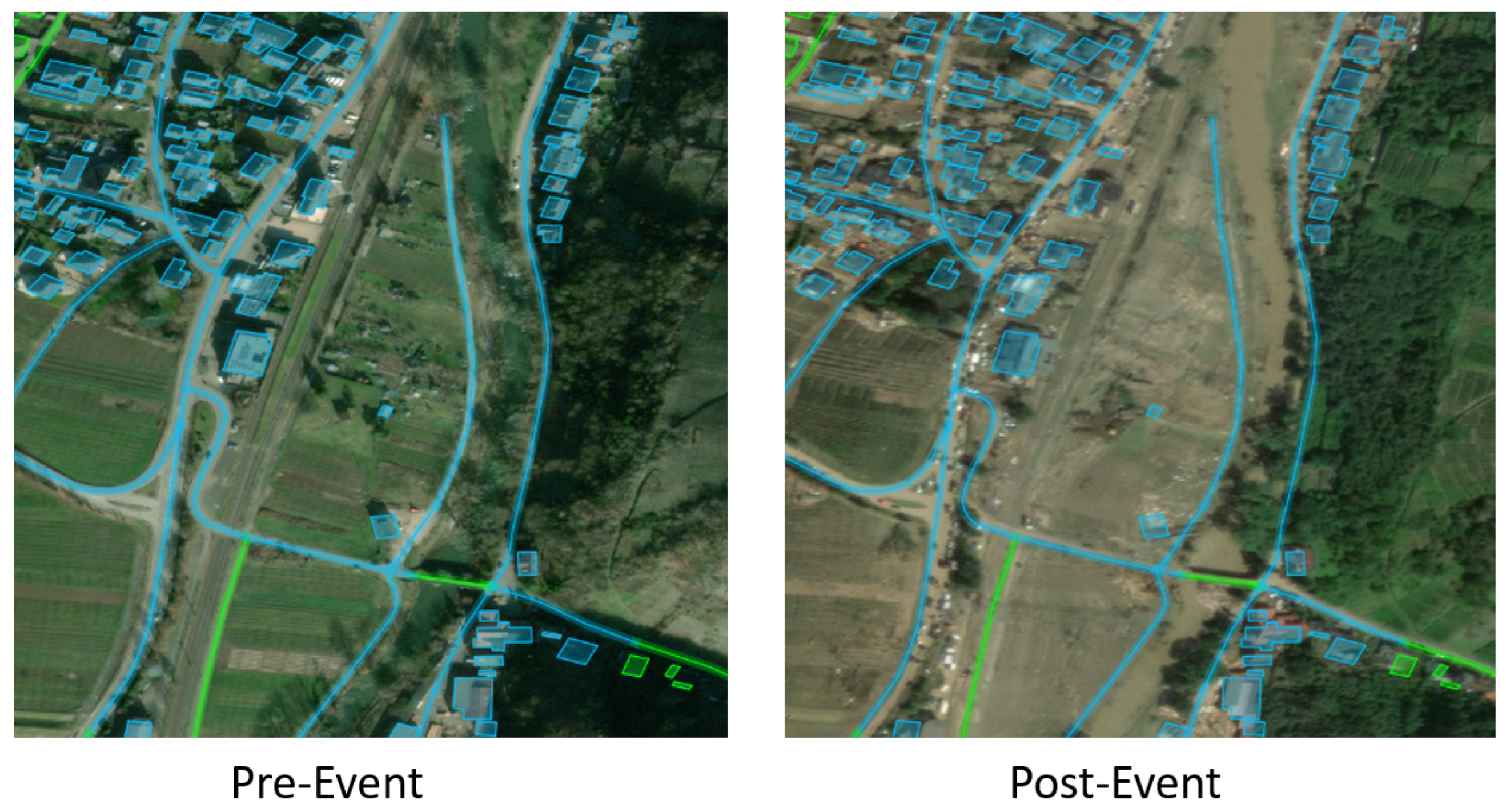
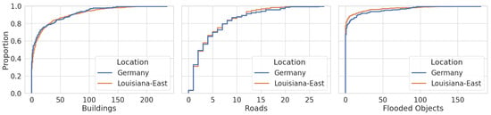
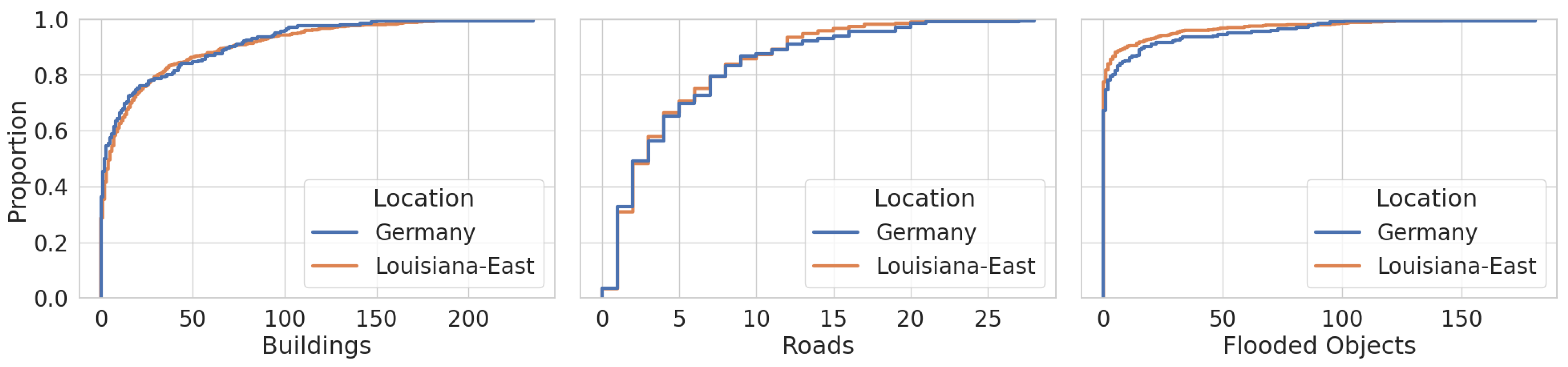
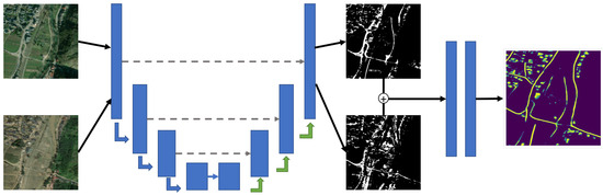
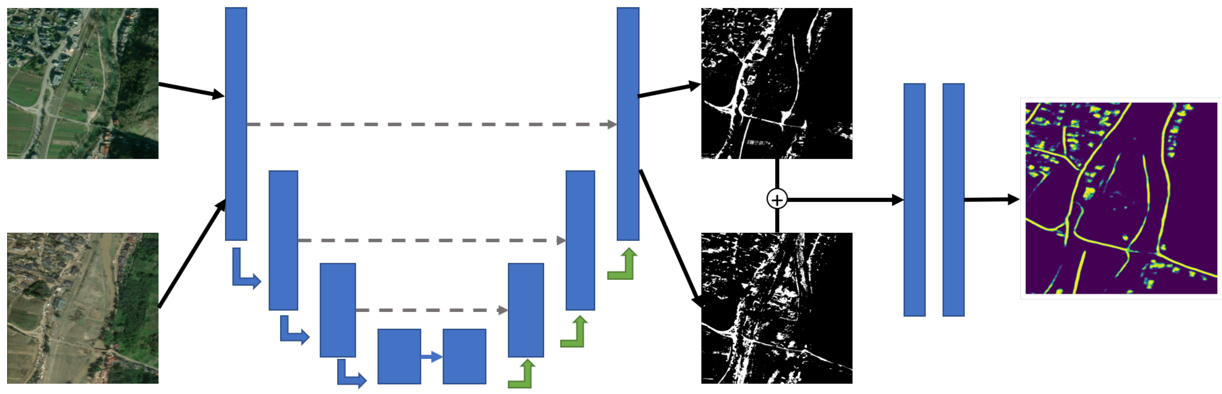
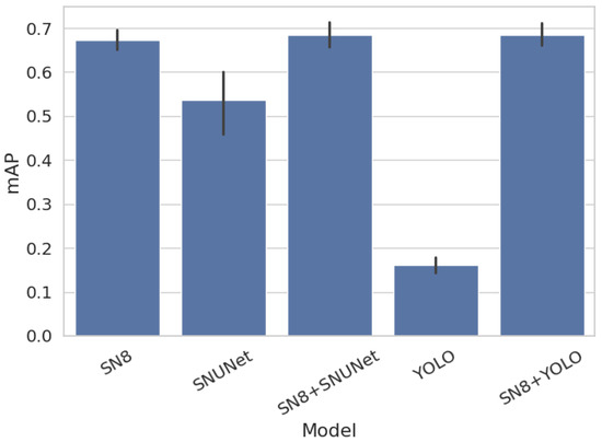
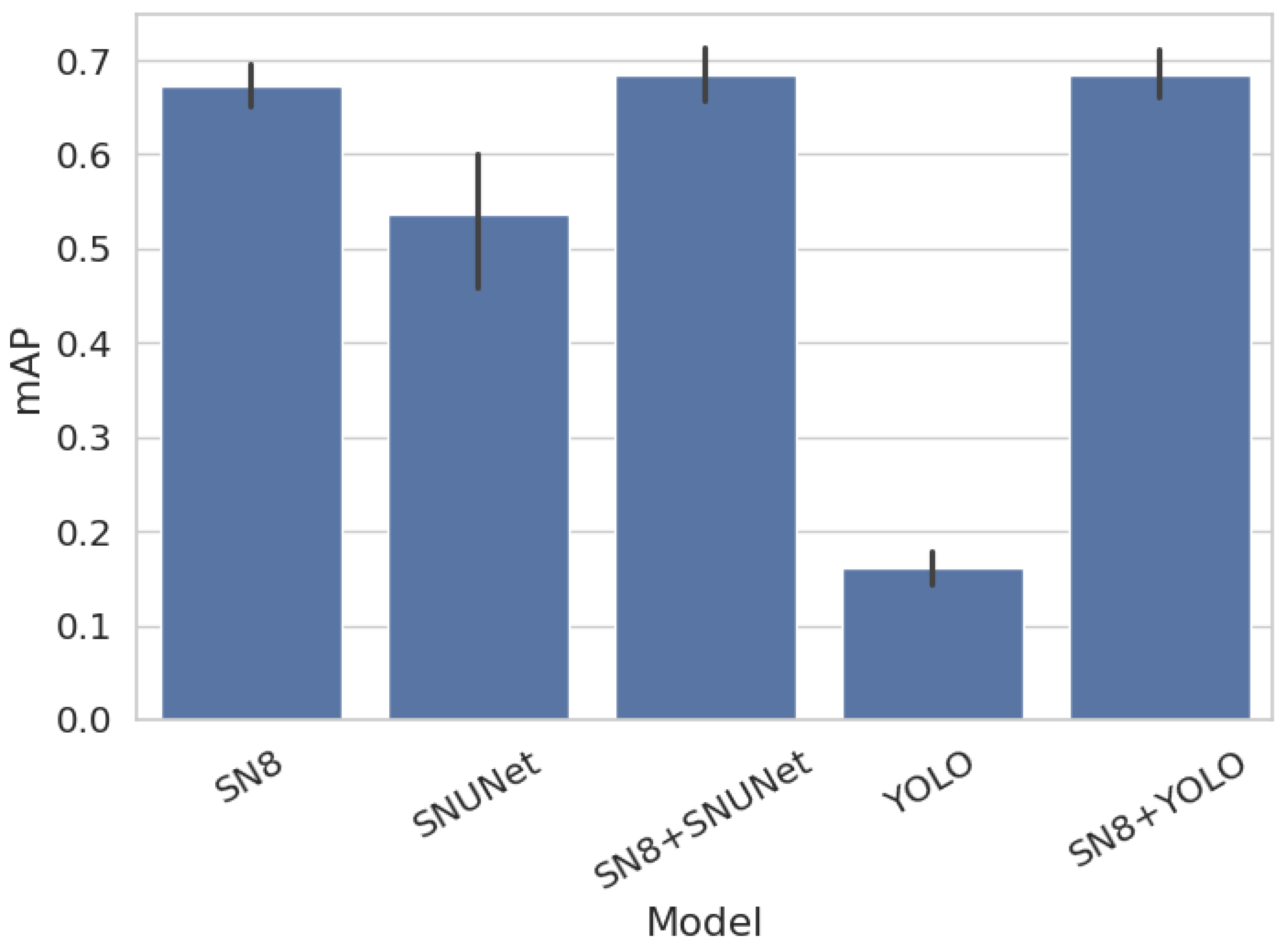
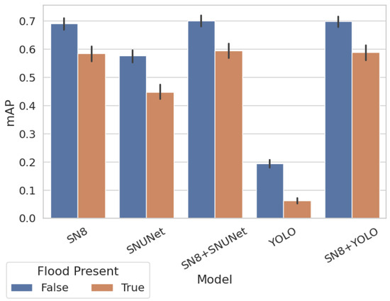
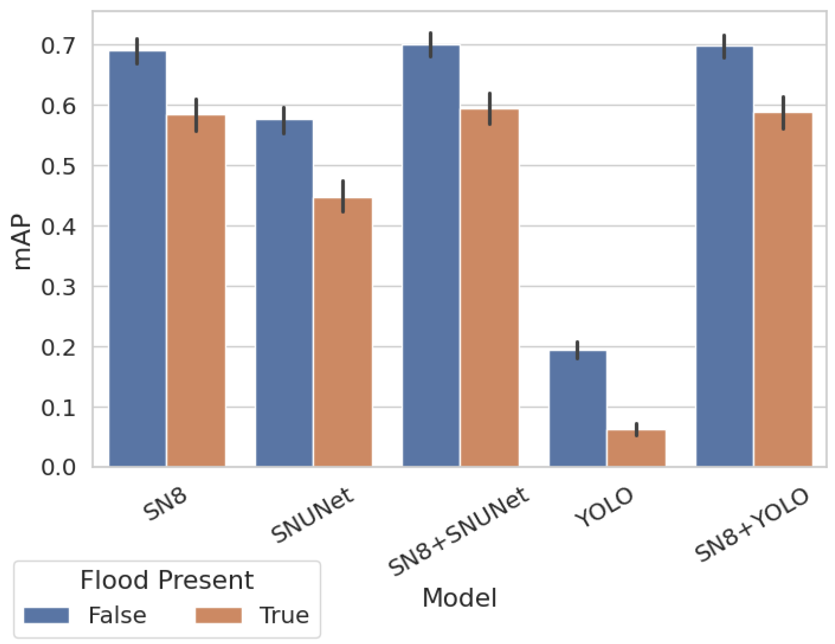
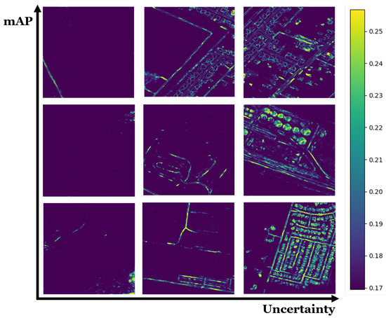
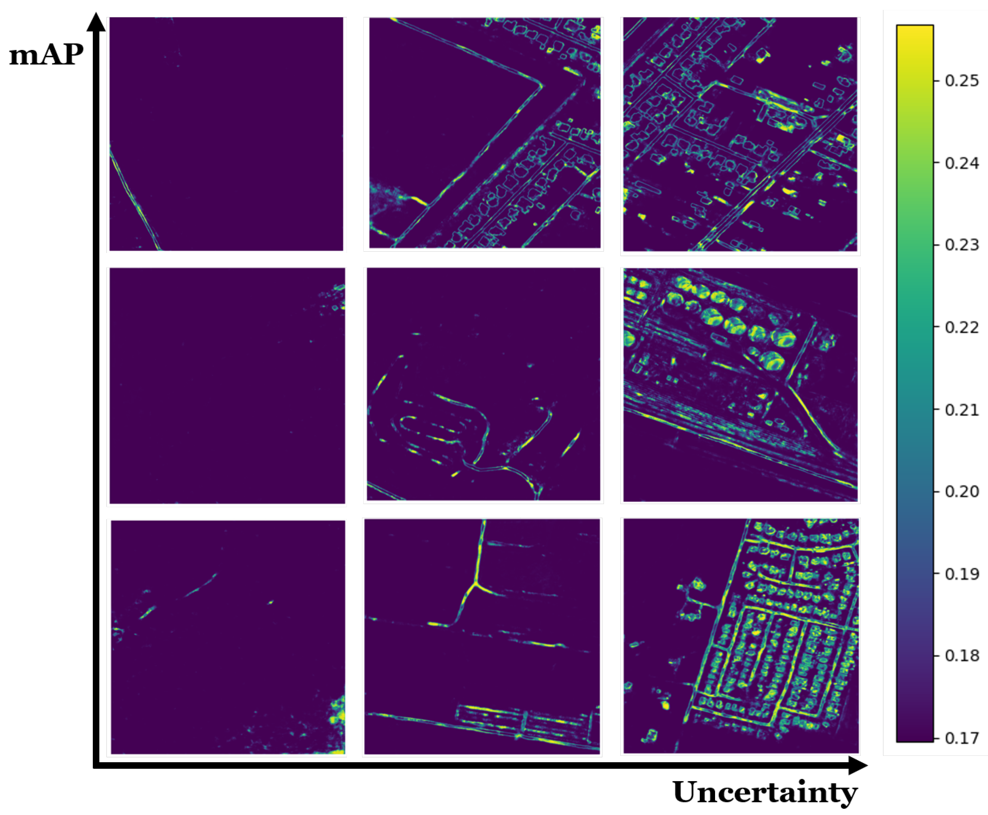
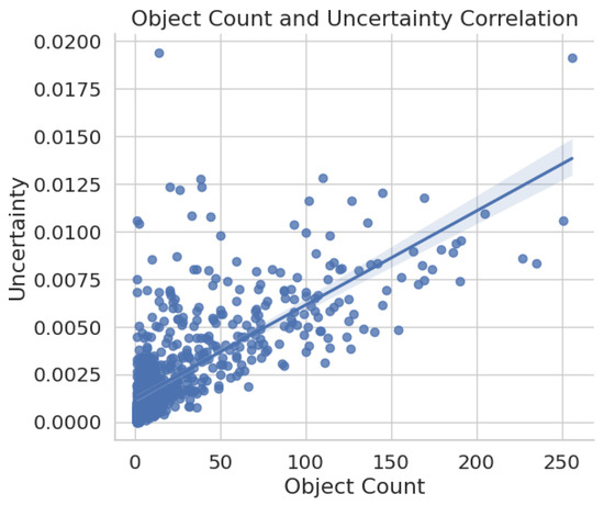
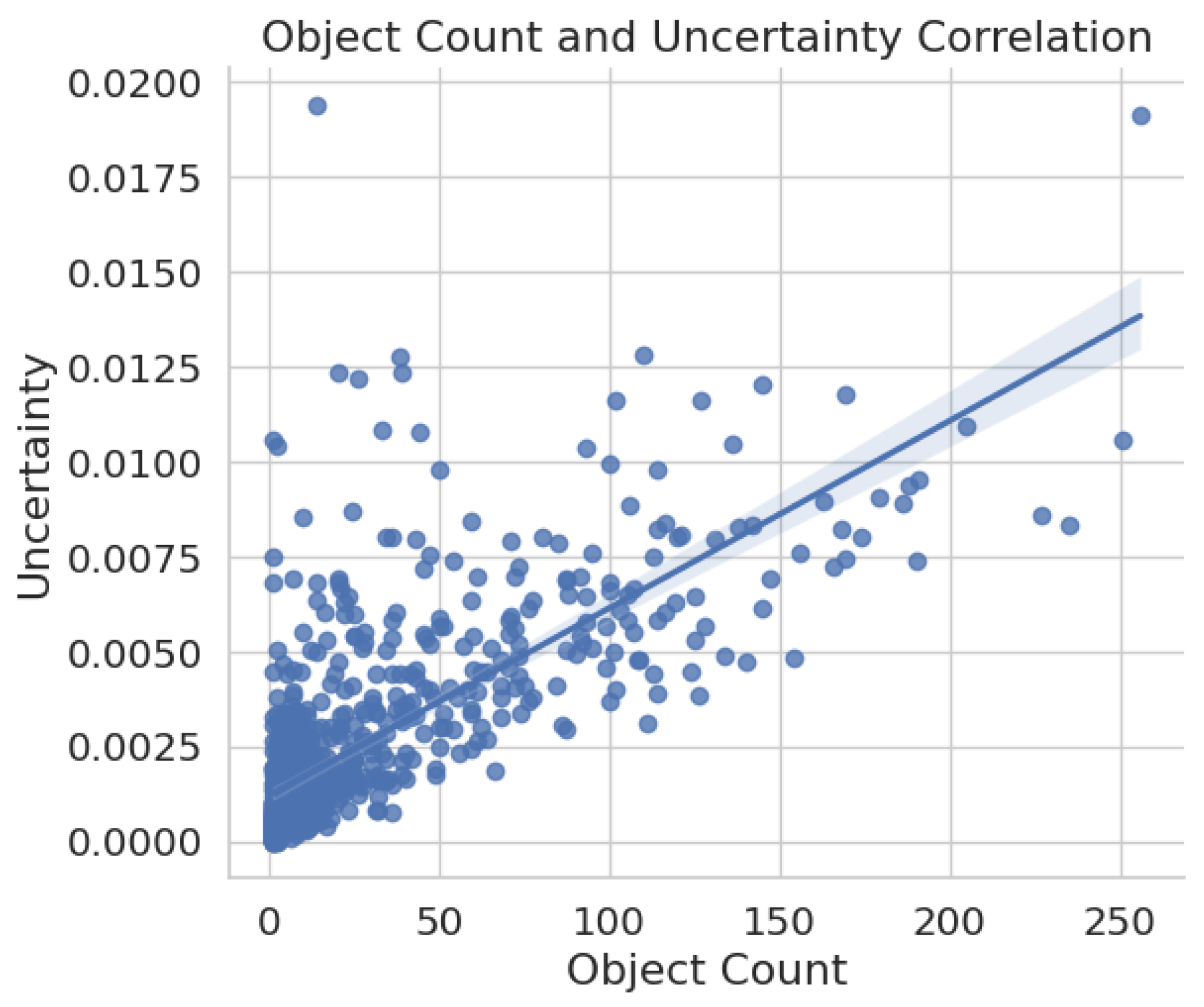
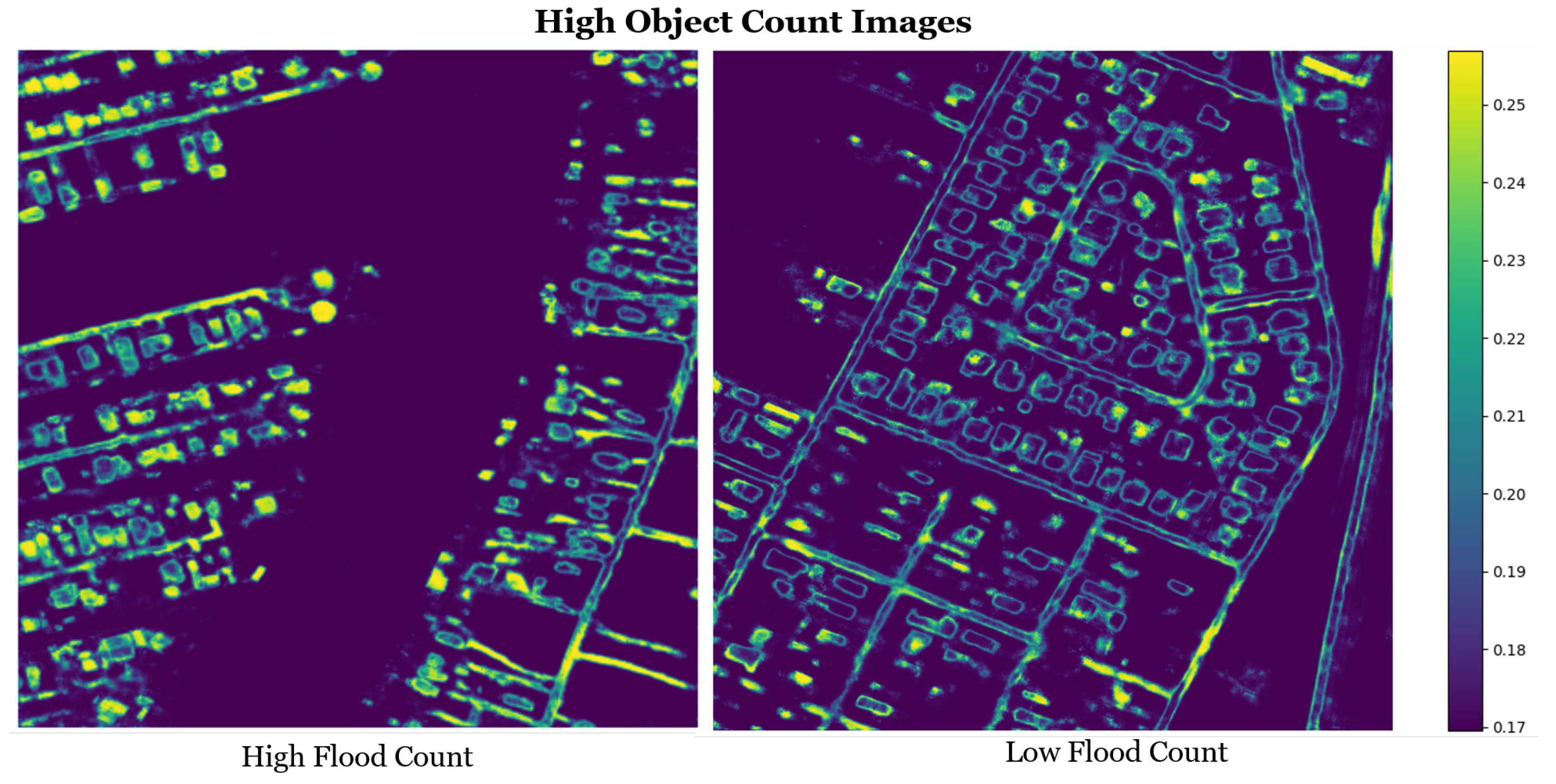
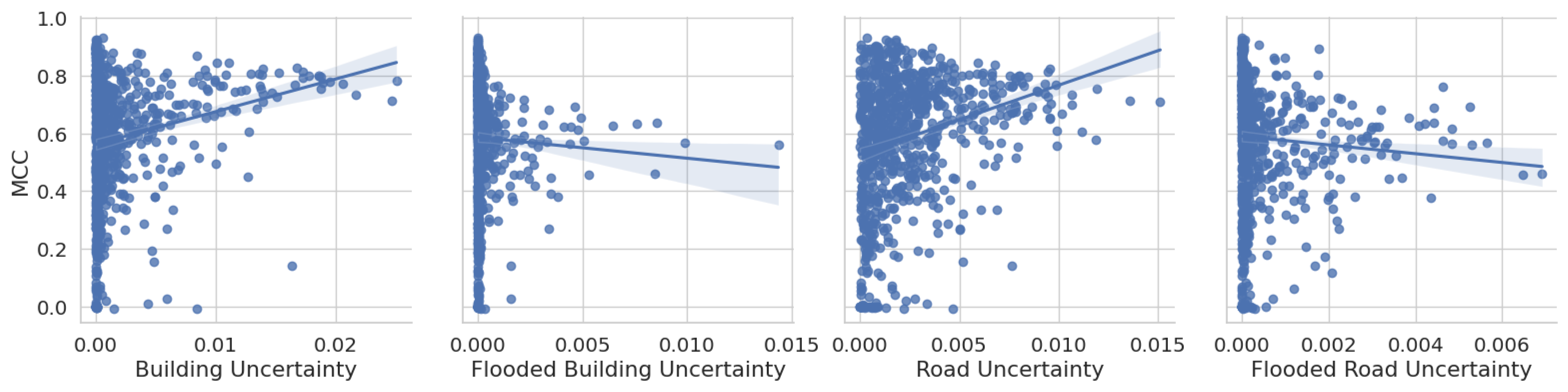

Disclaimer/Publisher’s Note: The statements, opinions and data contained in all publications are solely those of the individual author(s) and contributor(s) and not of MDPI and/or the editor(s). MDPI and/or the editor(s) disclaim responsibility for any injury to people or property resulting from any ideas, methods, instructions or products referred to in the content. |
© 2026 by the authors. Licensee MDPI, Basel, Switzerland. This article is an open access article distributed under the terms and conditions of the Creative Commons Attribution (CC BY) license.