


Highlights
What are the main findings?
- Identification of the optimal time-window combination for Soil Salinity Content (SSC) retrieval. Leveraging the Google Earth Engine (GEE) platform, this study systematically evaluated various time-window and image composition strategies. The results indicate that the Median composition strategy utilizing data from the preceding growing season (July–September) represents the optimal approach for retrieving spring soil salinity in the Yellow River Delta.
What are the implications of the main findings?
- Elucidation of the Mechanism for Predicting Subsequent Year Salinity Using “Legacy” Vegetation Signals. The study reveals a strong correlation between the spectral characteristics of vegetation from the preceding growing season and top SSC in the subsequent spring. This suggests that variations in vegetation growth induced by summer salt stress—such as reduced chlorophyll content and altered canopy structure—serve as stable “legacy signals” that effectively reflect background soil salinization levels.
- Proposal of a New Paradigm for Salinization Early Warning. Distinct from traditional “instantaneous monitoring,” this study proposes an early warning framework based on historical vegetation stress features. We demonstrate that predicting spring soil salinization risk using remote sensing data from the previous year—prior to spring crop canopy closure—is both feasible and highly accurate. This provides a critical time lead for precision management in agricultural irrigation districts.
Abstract
Soil salinization is a primary bottleneck for the sustainable development of agriculture in the Yellow River Delta (YRD). Conventional remote sensing monitoring predominantly relies on single-phase instantaneous spectral responses, which are highly vulnerable to transient environmental interferences, such as surface moisture fluctuations. This study proposes a novel predictive framework based on legacy vegetation signals. By integrating multi-temporal Sentinel-2 imagery from the 2024 growing season, we quantified the cumulative physiological feedback of crops from the preceding year and developed a spring soil salinity content (SSC) inversion model for 2025 using the LightGBM algorithm. The results demonstrate that the median compositing technique significantly enhances model robustness against outliers. Furthermore, the optimal time window for capturing these legacy signals for spring salinity monitoring was identified as July to September. Compared with traditional immediate monitoring models, the LightGBM model based on previous-season legacy signals achieved superior predictive accuracy (R2 = 0.84), effectively mitigating the impact of stochastic noise. This research validates the critical role of long-term vegetation memory in salinity early warning and provides a robust scientific foundation for the precision management of coastal saline-alkali land.
1. Introduction
Soil salinization is a pervasive environmental challenge that threatens global ecological stability. In China, saline-alkali land spans approximately 9.21 million hectares, accounting for 6.62% of the total cultivated area [1]. This phenomenon not only severely impedes the sustainable development of agricultural production but also jeopardizes regional ecological security. Globally, over 100 countries face challenges related to soil salinization, and it is estimated that by 2050, 50% of the world’s cultivated land will be affected by salinization [2]. This vulnerability is particularly pronounced in complex coastal wetland environments, such as the Yellow River Delta (YRD), where dynamic salinity fluctuations significantly compromise ecosystem balance and agricultural productivity [3]. The salinization crisis in the YRD is singularly acute, with saline-alkali soils covering approximately 442,900 hectares—of which 236,300 hectares are classified as severely salinized or barren [4]. Such extensive degradation severely curtails local agricultural output and adversely impacts biodiversity and ecosystem health [5]. Consequently, accurate monitoring and assessment of soil salinization are imperative for formulating effective land management strategies and ensuring food security.
Traditionally, the determination of soil salt content (SSC) has relied heavily on field sampling and laboratory chemical analysis. Although these methods offer high precision, they are inherently time-consuming and labor-intensive, precluding large-scale and high-frequency monitoring [6,7,8]. In recent years, the rapid proliferation of remote sensing technology—specifically advancements in proximal, satellite, and airborne sensing—has catalyzed novel solutions for efficient, accurate, and periodic salinity monitoring [9]. For instance, diagnostic spectral bands and salinity parameters have been identified using UAV imagery and in situ measurements, with their efficacy verified via Grey Relational Analysis (GRA) and Pearson correlation coefficients [10]. Furthermore, satellite platforms like Landsat 8 and Sentinel-2 have been extensively deployed for electrical conductivity (EC) mapping due to their spectral diversity and cost-effectiveness, which are pivotal for understanding soil genesis and optimizing agricultural management [9]. The integration of multi-scale platforms with ground observations has proven instrumental in enhancing inversion accuracy [11]. By fusing multi-platform data, researchers can mitigate the limitations of single data sources and more comprehensively capture the spatial variability and dynamic characteristics of soil salinity [12]. Notably, advancements in artificial intelligence have further facilitated the extraction of critical insights from massive, multi-source datasets.
Machine learning provides a robust and high-precision framework for integrating multi-source remote sensing data and modeling complex non-linear relationships. By leveraging the advantages of machine learning, researchers can significantly enhance the reliability and accuracy of soil salinity estimations [12]. Ensemble learning models, in particular, exhibit exceptional performance due to their capacity to effectively capture the intricate non-linear interactions between spectral information and salinity gradients [13]. The pedogenesis of soil salinization is inherently complex, with spectral signatures susceptible to the confounding influences of soil texture, soil organic matter (SOM), and moisture content. Consequently, characterizing salinity through a single variable remains arduous, and linear models typically yield subpar results in regions with high spatial heterogeneity [14,15]. While algorithms like Support Vector Regression (SVR), Random Forest (RF), and Extremely Randomized Trees (ET) have achieved high accuracy across various regions [13,16], their predictive stability can fluctuate under different environmental conditions. Thus, evaluating the performance of multiple regression algorithms is pivotal for constructing adaptive and reliable prediction models [1]. Despite the success of Artificial Neural Networks (ANNs) and Multivariate Adaptive Regression Splines (MARS), the influence of multi-temporal satellite observations across distinct phenological stages is frequently marginalized. In contexts where variables like soil moisture, vegetation cover, and surface roughness change dynamically, single-phase data often struggle to capture the comprehensive spectral response of soil salinity [12]. Traditional ‘immediate monitoring’ primarily relies on the concurrent spectral response of soil and sparse early-spring vegetation. However, such methods are frequently compromised by short-term hydro-meteorological noise, such as transient surface moisture from snowmelt. In contrast, the ‘legacy vegetation signal’ method leverages the cumulative physiological feedback of crops from the preceding peak growing season. This approach provides a more stable and representative characterization of the soil’s intrinsic saline-alkali status, effectively decoupling the long-term salinity influence from instantaneous environmental interference. Remote sensing inversion of soil salinity faces multifaceted challenges, including scale effects derived from varying spatial resolutions and seasonal fluctuations in salt concentration. These complexities necessitate more refined data selection and modeling strategies. Consequently, leveraging multi-temporal remote sensing data is paramount for capturing seasonal dynamic variations and performing targeted model optimization, which is essential for enhancing the accuracy and timeliness of regional salinization monitoring [3].
To address these challenges, this study proposes an integrated research approach to characterize soil salinity dynamics in the Yellow River Delta. Specifically, we developed a modeling framework that bridges the gap between historical vegetation performance and current soil states. Using multi-temporal Sentinel-2 imagery, we first extracted a suite of spectral indices to quantify ‘legacy vegetation signals’ from the previous growing season. Subsequently, these legacy features, alongside instantaneous environmental variables, were integrated into machine learning architecture. By systematically comparing the performance of legacy-based and instantaneous-based models, we aimed to validate whether long-term vegetation memory provides a more robust proxy for spring salinity early warning. The results are expected to provide new theoretical insights and technical support for regional soil degradation monitoring.
2. Materials and Methods
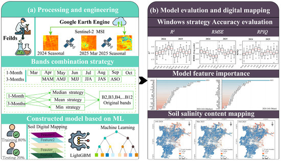
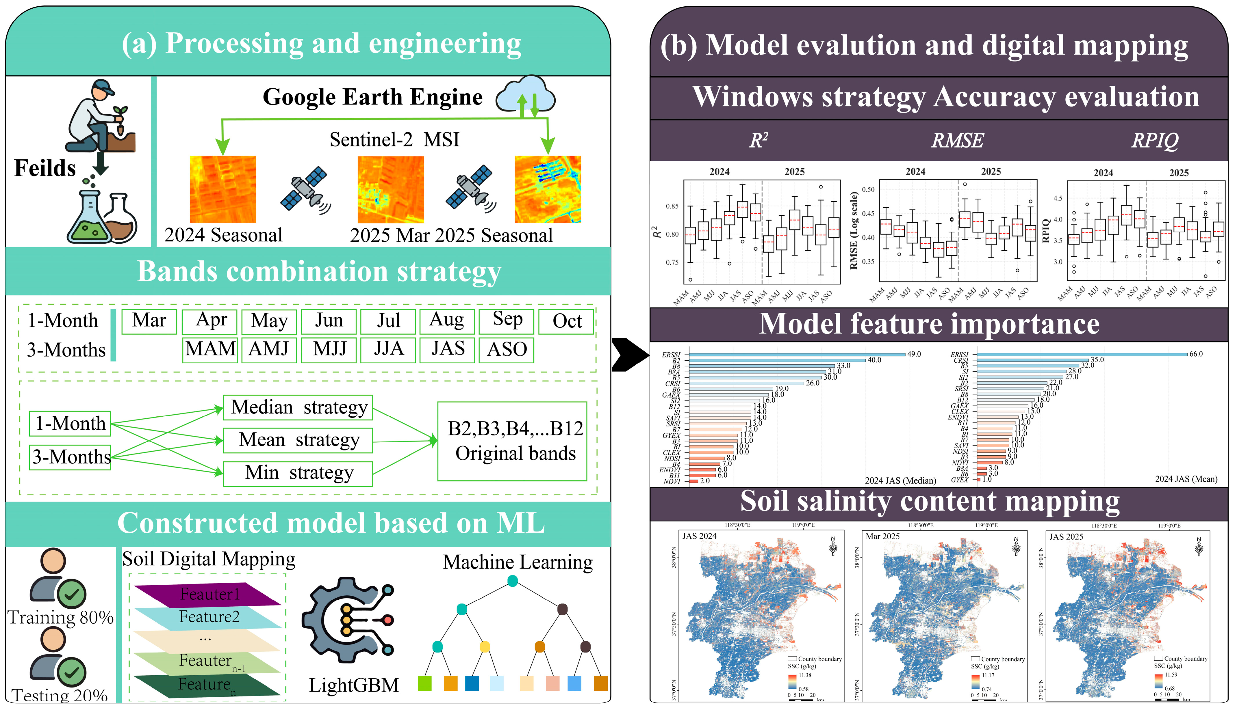
The research framework was established around two pivotal phases: (1) remote sensing data preprocessing and feature engineering and construction of data composition strategies across varying time windows; (2) model accuracy assessment and spatial analysis of the results. The schematic representation of this methodological workflow is illustrated in Figure 1, while comprehensive technical specifications for each phase are detailed in the subsequent sections.
Figure 1.
Flowchart of the research framework. The acronyms MAM, AMJ, MJJ, JJA, JAS, and ASO denote the 3-month rolling windows of March–May, April–June, May–July, June–August, July–September, and August–October, respectively. (a) The satellite data acquisition, time-window composition strategy, and modeling workflow; (b) Model evaluation and soil salinity content mapping result.
2.1. Study Area
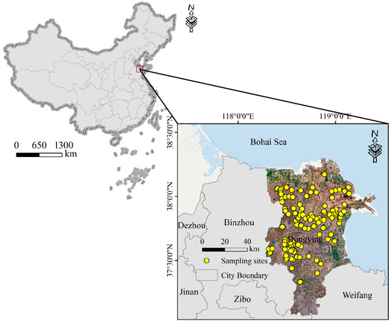
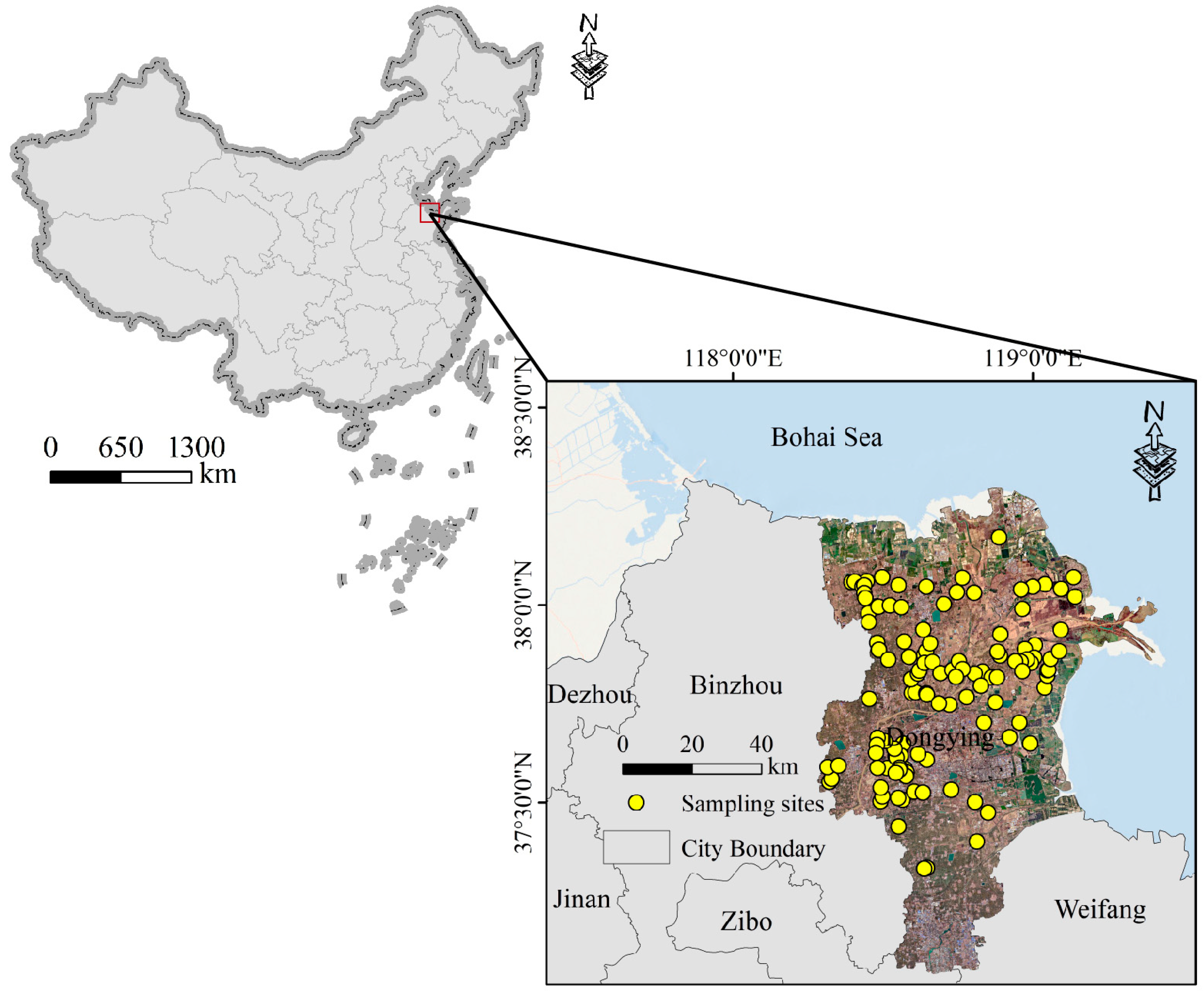
The study area is situated on the west coast of the Bohai Sea (118°6′–119°18′ E, 36°56′–38°8′ N) (Figure 2), characterized as the youngest wetland ecosystem globally. The Yellow River Delta (YRD) was formed through the interaction among river, sea, and land. This region belongs to a warm temperate continental monsoon climate [17]. An annual average temperature of 12.2 °C is recorded, accompanied by unstable interannual precipitation. The annual evaporation in this region exceeds rainfall, by which the upward movement of soil salts is induced, resulting in seasonal re-salinization and desalination. The seasonal dynamics of soil salinity are primarily manifested as accumulation in spring, leaching in summer, resurgence in autumn, and preservation in winter [3]. The dominant soil types are identified as Solonchaks and Fluvo-aquic soils, accounting for 80% of the total soil types. Following the diversion of the Yellow River in 1855, the river flowed into the Bohai Sea, whereby a typical alluvial fan estuarine wetland was formed [18].
Figure 2.
Schematic diagram of the study area location.
2.2. Soil Sampling and Laboratory Analysis
Field soil sampling was conducted from 18 to 23 March 2025. During the spring (March), driven by intense evaporative demand, salts migrate upward from the shallow groundwater, leading to pronounced salinity accumulation in the topsoil. This period represents a critical phase for salt buildup in the 0–20 cm layer, enabling the capture of peak salinity levels that are essential for evaluating ecological management and agricultural practices [19]. A random sampling strategy was implemented to capture the significant spatial heterogeneity of soil salinity across the region. This design comprehensively integrated known land-use types, vegetation characteristics, distance from the coastline, and the spatial patterns of salinity gradients. A total of 119 soil sampling sites were established to represent the predominant landscape patterns of the Yellow River Delta, encompassing irrigated agricultural lands, saline-alkali wastelands, and coastal wetlands. Among these, 72 sites were located in areas covered by winter wheat, crop residues, and deep-plowed soil, while the remaining 47 sites were situated in saline-alkali bare lands and sparsely vegetated areas. This distribution ensures a comprehensive representation of the region’s diverse land-use types and salinity gradients. A 1:5 soil–water extract was prepared by mixing 20 g of the treated soil with 100 mL of distilled water. The electrical conductivity (EC 1:5) was measured using a DOS-307A conductivity meter. The concentrations of carbonate () and bicarbonate () were determined via neutralization titration. Chloride () content was measured using silver nitrate () titration, while sulfate () was quantified through the turbidimetric method. Additionally, the base cations, including potassium (), sodium (), magnesium (), and calcium (), were analyzed using Inductively Coupled Plasma Atomic Emission Spectrometry (ICP-AES), while the total SSC was calculated based on the sum of ions determined using an ICP-AES Avio 550 Max system. The empirical relationship between electrical conductivity EC (1:5) and total soil salt content (SSC) used in this study is expressed as follows:
SSC (g/kg) = 2.6157 × EC (1:5) + 0.3504
2.3. Remote Sensing Data Preprocessing
Soil salinity is influenced by the synergistic effects of various pedogenic factors, including parent material, climate, relief, and organisms. In Digital Soil Mapping (DSM), the selection of environmental variables necessitates that these factors be directly or indirectly represented [20]. In this study, remote sensing data processing was implemented on the Google Earth Engine (GEE) cloud platform. We utilized Sentinel-2 Level-2A surface reflectance products, which have undergone orthorectification and atmospheric correction via the Sen2Cor algorithm. Remote sensing imagery is frequently compromised by interference from clouds, cloud shadows, aerosols, and sensor noise, which can result in anomalous pixel values. Notably, the maximum values of original spectral bands are particularly susceptible to cloud contamination [21]. To ensure data integrity, a rigorous preprocessing workflow was executed:
Cloud Masking: Opaque clouds, cirrus, and cloud shadows were masked using the QA60 band in conjunction with the Scene Classification Layer (SCL).
Temporal Compositing: For each defined rolling window (1-month and 3-month), image aggregation was performed using median, mean, and minimum (Min) compositing functions.
A research framework for soil mapping was constructed based on a systematically collected suite of spectral indices. Subsequently, these three compositing methods were employed to calculate characteristic spectral indices (Table 1). The original spectral bands and derived indices were integrated into a feature dataset, serving as the input predictor set for the model.
Table 1.
Predictor variables for soil salinity: abbreviations, calculation formulas, and references.
2.4. Composition Strategies
The implementation of 1-month and 3-month rolling windows was strategically designed to align with the distinct temporal scales of water-salt transport in the Yellow River Delta. The 1-month window is tailored to capture short-term, pulse-like fluctuations in salinity driven by discrete events, such as intensive rainfall or irrigation leaching, thereby reflecting the immediate hydrodynamic response of the topsoil. In contrast, the 3-month window corresponds to the cumulative duration of major phenological stages, facilitating the integration of long-term physiological feedback from vegetation to persistent osmotic stress. Consequently, these multi-scale temporal compositing strategies were adopted to enhance the characterization of soil salinity dynamics. In consideration of the legacy features and lag effects of salinization, a multi-temporal compositing method was defined to predict soil salinity. This method incorporates data from the growing season of the preceding year and the concurrent growing season prior to crop canopy closure, aiming to evaluate the optimal time-window and compositing strategy for monitoring coastal soil salinization. The specific procedures are as follows:
Data Acquisition: All Sentinel-2 imagery with low cloud cover (<20%) covering the study area from March to October in both 2024 and 2025 was acquired.
Compositing Strategy: Based on ten optical bands of Sentinel-2 (Bands 2, 3, 4, 5, 6, 7, 8, 8A, 11, and 12), bands frequently utilized for soil monitoring and vegetation feature identification were selected. During the growing season from March to October, complete surface reflectance datasets were constructed using 1-month and 3-month rolling time windows (specifically, MAM, AMJ, MJJ, JJA, JAS, and ASO). The impacts of compositing strategies on model performance were compared within the Google Earth Engine (GEE) platform using various strategies across different temporal scales, encompassing a total of 66 distinct strategy models.
1-month temporal scale: The accuracy of soil salinity models was evaluated using three compositing strategies. Considering both the year preceding canopy closure and the concurrent growing season, 16 scenarios were evaluated for each compositing strategy.
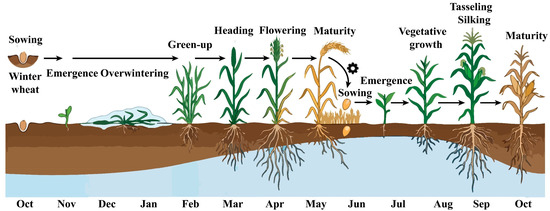
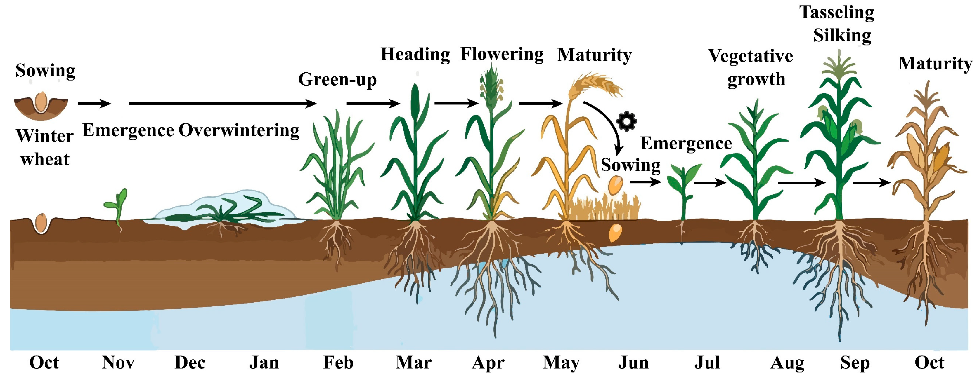
3-month temporal scale: The compositing strategies included 12 scenarios. This combinatorial strategy was established in consideration of the Winter Wheat-Summer Maize rotation characteristics in the North China Plain during the growing season (March–October). It fundamentally reflects the phenological stages of local major crops, covering critical periods such as the emergence, greening, jointing, heading, flowering, and maturity of winter wheat, as well as the seedling, jointing, tasseling, flowering, and maturity stages of maize. The schematic diagram is shown in Figure 3.
Figure 3.
Schematic diagram of the wheat-maize rotation cycle.
2.5. Prediction Models and Model Evaluation Criteria
Compared to traditional models, the LightGBM model is a highly efficient variant of the Gradient Boosting Decision Tree (GBDT) framework. It employs a leaf-wise growth strategy with a defined maximum depth constraint, which, compared to the conventional level-wise approach, focuses on splitting leaf nodes with the highest gain for a given number of iterations. Research indicates that LightGBM typically outperforms the traditional machine learning models in both accuracy and computational efficiency, making it particularly suitable for digital soil mapping scenarios involving high-dimensional, multi-source remote sensing data. This strategy allows for more effective loss reduction and a significant enhancement in inversion precision [31,32].
In this study, the LightGBM model was selected for its superior efficiency and accuracy in handling complex non-linear relationships. To ensure high reproducibility and model stability, the following standardized protocols were implemented:
The calculation formulas for the assessment metrics are as follows:
(1) Data Preprocessing: A log-transformation was applied to the raw SSC data to mitigate the effects of high spatial heterogeneity and skewed distribution.
(2) Feature Engineering: Twenty-three predictor variables, including original spectral bands and derived vegetation/salinity indices, were standardized as model inputs.
(3) Hyperparameter Tuning: To optimize the model performance, the number of estimators was set to 100, and a fixed random seed was employed to ensure reproducibility. Key hyperparameters, including the learning rate, number of leaves (num_leaves), and feature fraction, were determined using a systematic Grid Search strategy within the Python 3.10.0 environment. This optimization process was coupled with 10-fold cross-validation, a systematic approach that ensures the model achieves optimal generalization while effectively mitigating the risk of overfitting.
(4) Model Training: The dataset (n = 119) was randomly partitioned into a training set (80%) and a validation set (20%).
To assess the structural stability of the model, each modeling scenario was repeated 30 times, and the mean values of the evaluation metrics (R2, RMSE, and RPIQ) were reported. The calculation formulas are as follows:
where n is the number of soil samples, is the situ measured SSC value, is the predicted value, is the interquartile range (IQR), which is the difference between the upper quartile (Q3) and the lower quartile (Q1).
3. Results
3.1. Descriptive Statistics of Soil Salinity
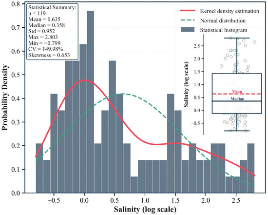
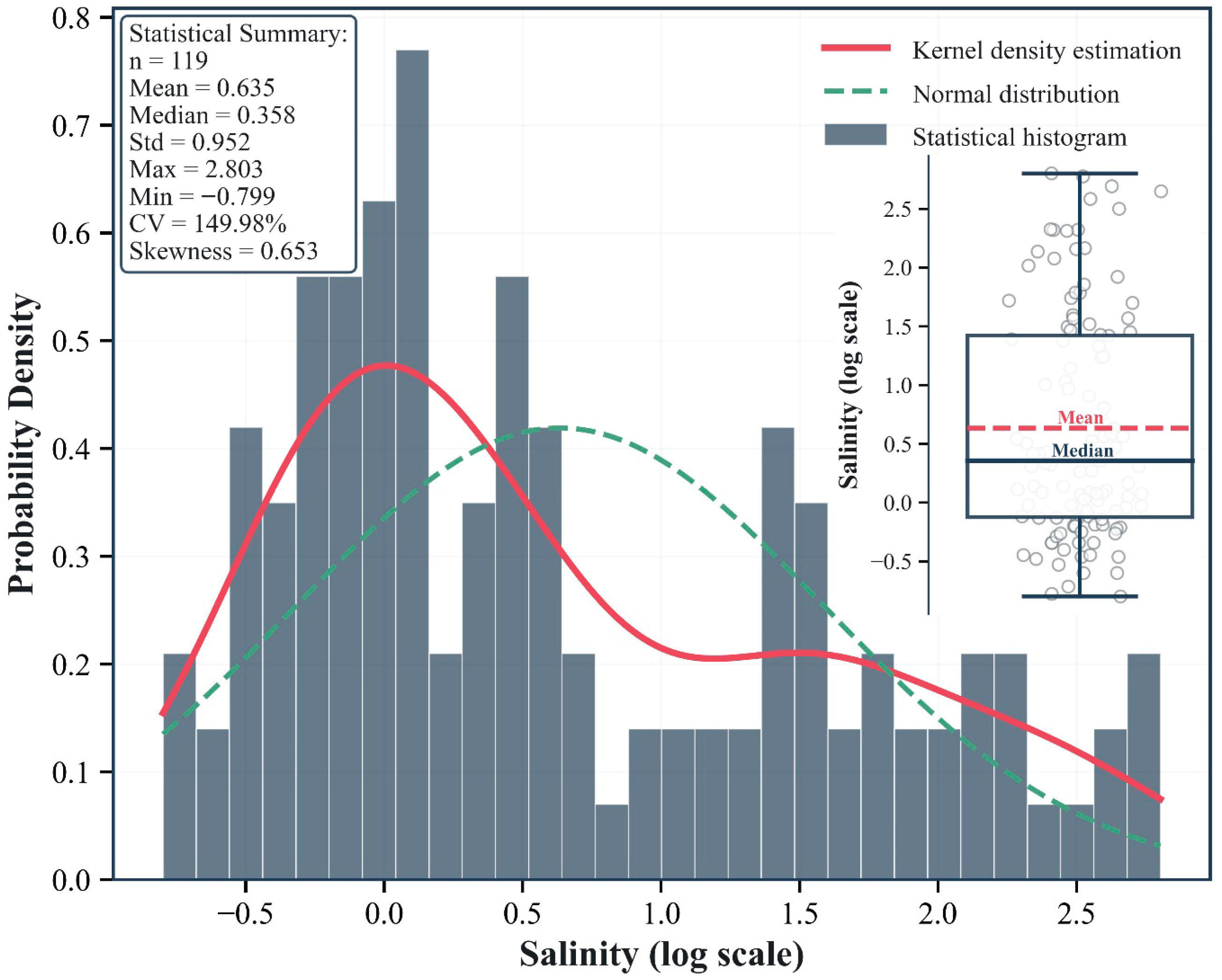
A log-transformation was applied to the soil salinity data derived from 119 samples, and their distribution characteristics were analyzed utilizing frequency histograms, Kernel Density Estimation (KDE), and boxplots (Figure 4). The sample data exhibited a Coefficient of Variation (CV) of 149.98% and a Standard Deviation (SD) of 0.952. The values covered a wide dynamic range from −0.799 to 2.803, with the mean (Mean = 0.635) being significantly higher than the median (Median = 0.358). The comparison between the KDE curve (solid red line) and the theoretical normal distribution curve (dashed green line) in Figure 4 demonstrated that the salinity data deviated significantly from the normality assumption. This observation was further corroborated by the skewness coefficient (Skewness = 0.653 > 0). Consequently, high spatial variability was exhibited by the samples.
Figure 4.
Statistical distribution and probability density characteristics of log-transformed salinity data. The main plot displays the frequency histogram of salinity (on a logarithmic scale), superimposed with the Kernel Density Estimation (KDE) curve (solid red line) and the theoretical normal distribution fitting curve (dashed green line). The inset (upper right) presents a Box-Jitter plot, visually illustrating the dispersion of sample points; the mean is represented by the dashed red line, while the median is denoted by the solid dark blue line. Detailed descriptive statistical metrics are listed in the statistical box in the upper left corner (sample size, n = 119).
3.2. Evaluation of the Composition Strategy
3.2.1. Evaluation of the One-Month Band Composition Strategy
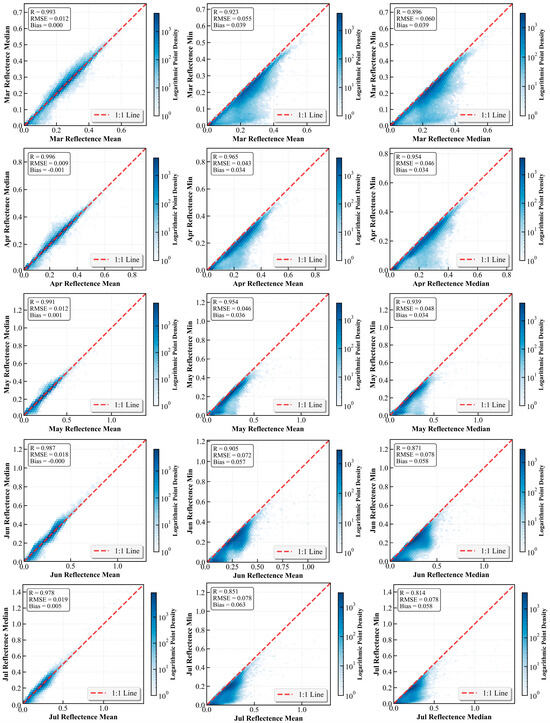
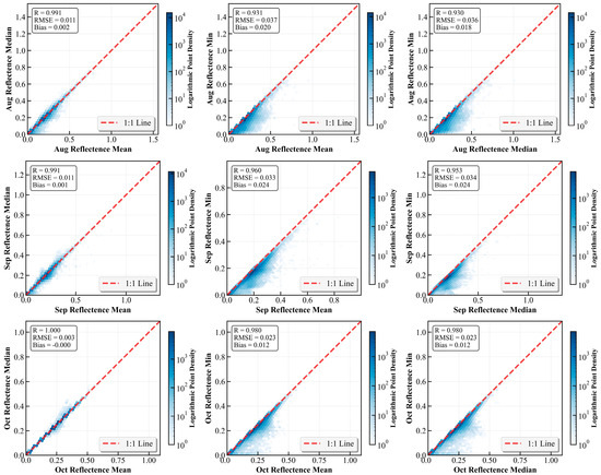
The objective of employing different compositing methods is to understand how various statistical metrics characterize the temporal stability of the land surface. The spectral response characteristics of soil salinity are primarily associated with surface moisture, salt crusts, and mineral composition. Previous studies have demonstrated that the Short-Wave Infrared (SWIR) bands exhibit a strong response to salt crystals and moisture content in the soil, possessing a clear physical relationship with soil salinity [33]. Consequently, Sentinel-2 SWIR bands were utilized to evaluate the effectiveness of different compositing strategies across various temporal scales. The results are presented in Figure 5, which illustrates the correlation analysis among mean, median, and minimum composites of reflectance bands during the growing season. Across all months, the mean and median composites exhibited an extremely high degree of consistency. Data points were tightly distributed around the 1:1 line without obvious dispersion, indicating that the difference between using the mean or median as a representative statistical metric for soil salinization monitoring in this region is negligible. Although the correlations between the minimum composite and the median/mean composites were significant, marked deviations and dispersion were observed. The vast majority of points were distributed below the 1:1 line; the correlation coefficient decreased, and the RMSE increased significantly. Furthermore, the degree of deviation varied across different months, reflecting the intra-unit heterogeneity of the observation units. The maximum dispersion between the minimum and median composites was observed in July (R = 0.814, RMSE = 0.078). Conversely, in October, a high degree of consistency was demonstrated among the three compositing methods; the R value for Min vs. Mean reached as high as 0.98, with an RMSE of only 0.023. At this stage, crops had been harvested or were senescent, resulting in strong surface homogeneity and weakened shadow effects, thereby causing the statistical metrics to converge.
Figure 5.
2D scatter density plots of SWIR for different composition strategies at the 1-month scale.
3.2.2. Evaluation of the Three-Month Band Composition Strategy
To evaluate the robustness of aggregation across different time windows, the results of distinct reflectance compositing strategies were compared across six rolling windows during the growing season (MAM, AMJ, MJJ, JJA, JAS, and ASO). Figure A1 illustrates the high degree of consistency between the mean and median composites within the 3-month time window; the Pearson correlation coefficient R exceeded 0.97, and the Root Mean Square Error (RMSE) remained below 0.024. This indicates that both median and mean reflectance metrics serve as reliable representatives for seasonal composite data. In contrast, higher variability was exhibited in the correlations of the minimum reflectance. Although a positive correlation was maintained (R values ranged from 0.738 to 0.893), distinct deviations were observed, with data points primarily clustered below the 1:1 line. Notably, these discrepancies exhibited a distinct seasonal dependency. The highest correlation was observed in the August–October (ASO) time window (maximum R = 0.887), whereas the weakest correlation occurred during the June–August (JJA) period (minimum R = 0.769). Higher RMSE values and lower correlations were observed during the summer months (specifically MAM, MJJ, and JJA), indicating that the minimum compositing strategy is more susceptible to noise or extreme variations during the growing season.
3.2.3. Evaluation of the One-Month Modeling Strategy
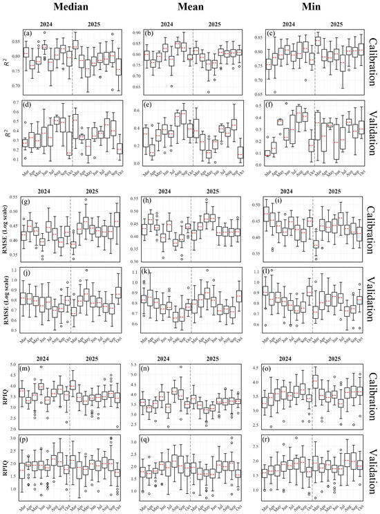
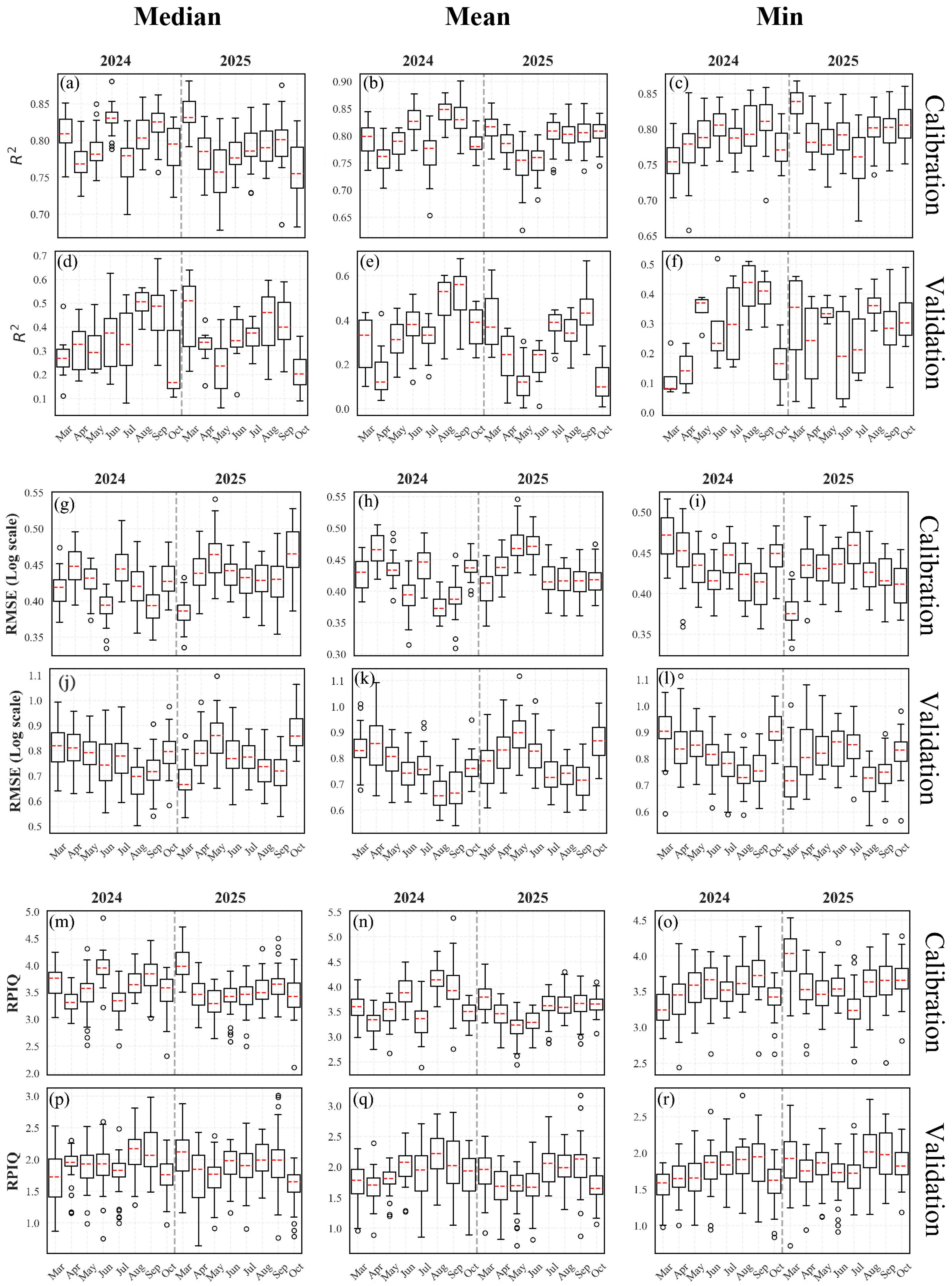
The performance of soil salinity inversion models, constructed based on spectral remote sensing indices across different time-window scales, is illustrated in Figure 6 for both the modeling and validation sets. Model performance was evaluated using the Coefficient of Determination (R2), the Root Mean Square Error (RMSE), and the Ratio of Performance to Interquartile Range (RPIQ). The results indicated that significant variability in model performance was exhibited across different months. It is noteworthy that, although the soil samples were collected in March 2025, higher prediction accuracies were achieved by models constructed using median or mean composited spectral data from the growing season of the preceding year (Figure 6d,e), particularly in August and September. The R2 values ranged from 0.45 to 0.60, with the lowest RMSE observed among all models, indicating the highest stability. The accuracy of these models was significantly superior to the performance of models constructed based on concurrent data from the sampling year.
Figure 6.
Evaluation of R2, RMSE, and RPIQ for models using 1-month composition strategies; (a–c,g–i,m–o) training set, (d–f,j–l,p–r) validation set.
3.2.4. Evaluation of the Three-Month Modeling Strategy
Overall, models across different time-window and compositing strategies exhibited significant seasonal variations and interannual differences. The coefficient of determination (R2) of the validation sets for different strategies ranged from 0.3 to 0.7 (Figure A2). Notably, the model based on the median composite of the July–September (JAS) period from the preceding year demonstrated superior generalization capability (Figure A2d).
While the model performance during the March–May (MAM) period of the preceding year was relatively weak, significant improvements were observed in the JAS and August–October (ASO) periods (Figure A2d,e). Acting as a salinity indicator, the signal of vegetation growth stress response tended to stabilize. The impact of soil salinization was indirectly reflected through vegetation growth status and the degree of stress. Following evapotranspiration in summer, salt accumulates on the surface due to water-salt dynamics. This phenomenon may be attributed to the temporal persistence of salt distribution, which influences the formation process of soil salinization in the following spring. This confirms that predicting soil salinity in the following spring using features from the peak growing season of the preceding year is feasible and potentially more robust than inversion based on the concurrent season.
Although the Mar 2025 period coincided with the sampling time and the modeling set performed acceptably (Figure A2d), the boxplots for MAM and April–June (AMJ) in the validation set typically exhibited larger variance and lower medians compared to those of the 2024 JAS period (Figure A2d). In early March, phenomena such as snowmelt, excessive soil moisture, or freeze–thaw cycles may occur on the land surface. The spectral absorption by water severely interferes with the spectral signals of salinity, leading to increased uncertainty in direct inversion; consequently, the modeling results based on spectral characteristics from the same period were inferior. Furthermore, due to the lack of vegetation cover in the spring of 2025, the spectral reflectance derived directly from bare soil, while direct, was highly susceptible to the influence of soil roughness and moisture. This resulted in substantial fluctuations in the accuracy of the validation set.
3.3. Time-Window and Variable Importance
Based on the modeling results derived from different time-window and composition strategies, the three optimal time windows were defined as follows: the concurrent window (based on synchronous satellite-ground observation during the sampling period in March 2025), the salinization legacy period of the growing season (July–September 2024), and the salinization stress period of the growing season (July–September 2025). Feature sets were constructed by integrating environmental factor characteristics synthesized via median and mean compositing.
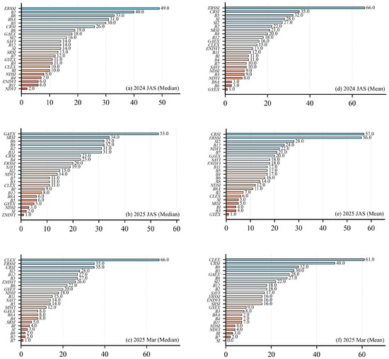
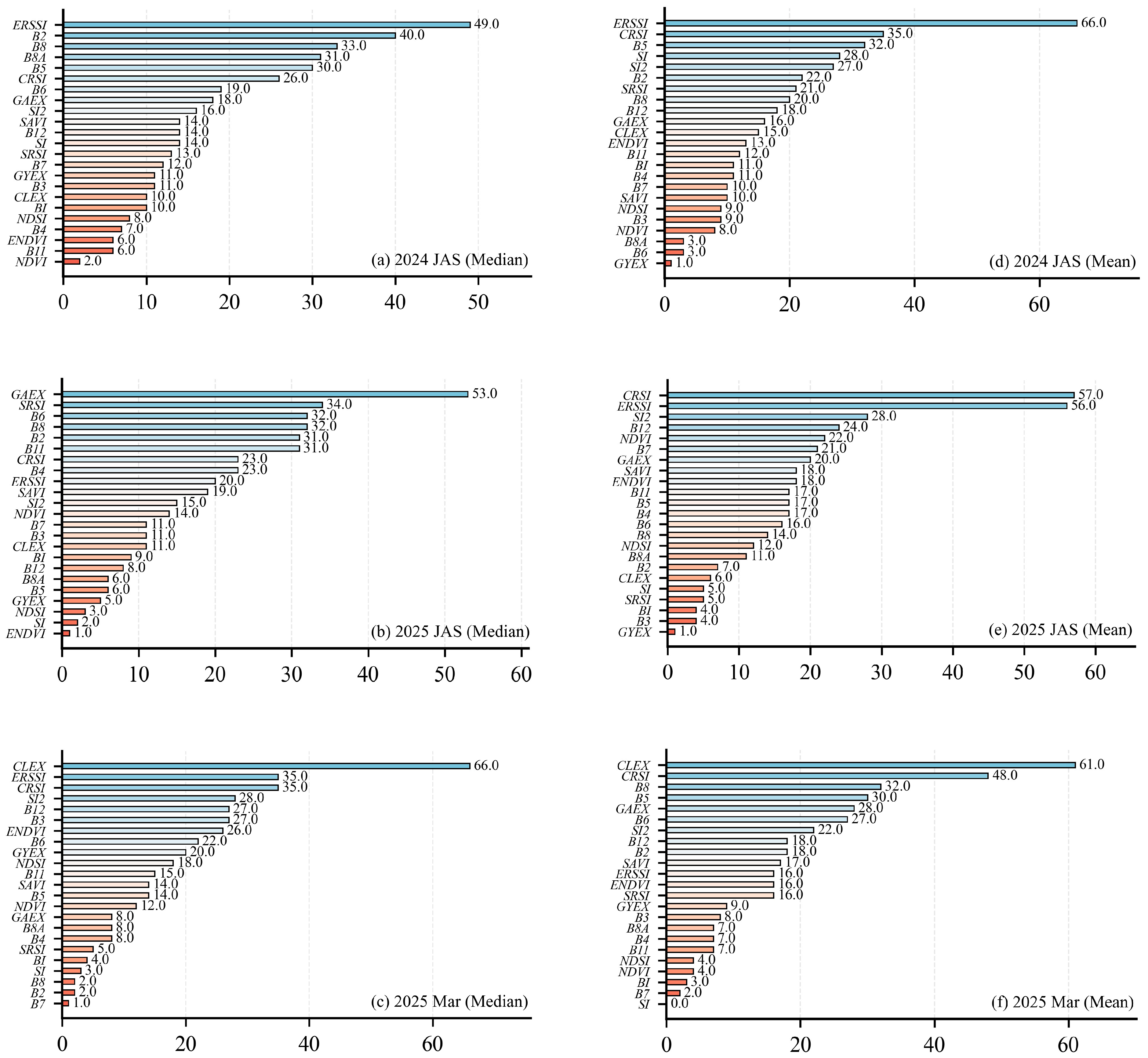
The contribution of each environmental variable to the modeling process was assessed through feature importance evaluation, and the differences in environmental variables generated across different time windows were analyzed. A higher importance value indicates a greater influence of the variable on the model. As illustrated in Figure 7, within the three datasets of different strategies, the contributions of environmental variables varied across different compositing methods within the same dataset; similarly, the contribution of the same environmental variable varied across different compositing strategies.
Figure 7.
Evaluation of feature importance for different time-window and composition strategies. (a,b,d,e) show the variable importance for the 3-month time-window with median and mean composite strategies; (c,f) show the variable importance for the 1-month time window with median and mean composite strategies.
However, commonalities were exhibited by certain environmental variables across different strategies. During the Salinization Legacy Period and the Stress Period, indices related to vegetation characteristics and canopy salinity response demonstrated shared patterns under different compositing strategies (Figure 7a,b). Conversely, in the single month of March (the concurrent window), indices associated with soil texture and soil conditions, such as CLEX, exhibited higher importance (Figure 7a,f). Furthermore, the importance of ERSSI, SRSI, and CRSI was observed to be generally high.
3.4. Prediction Evaluation
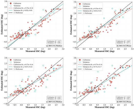
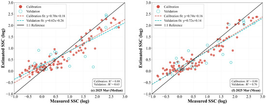
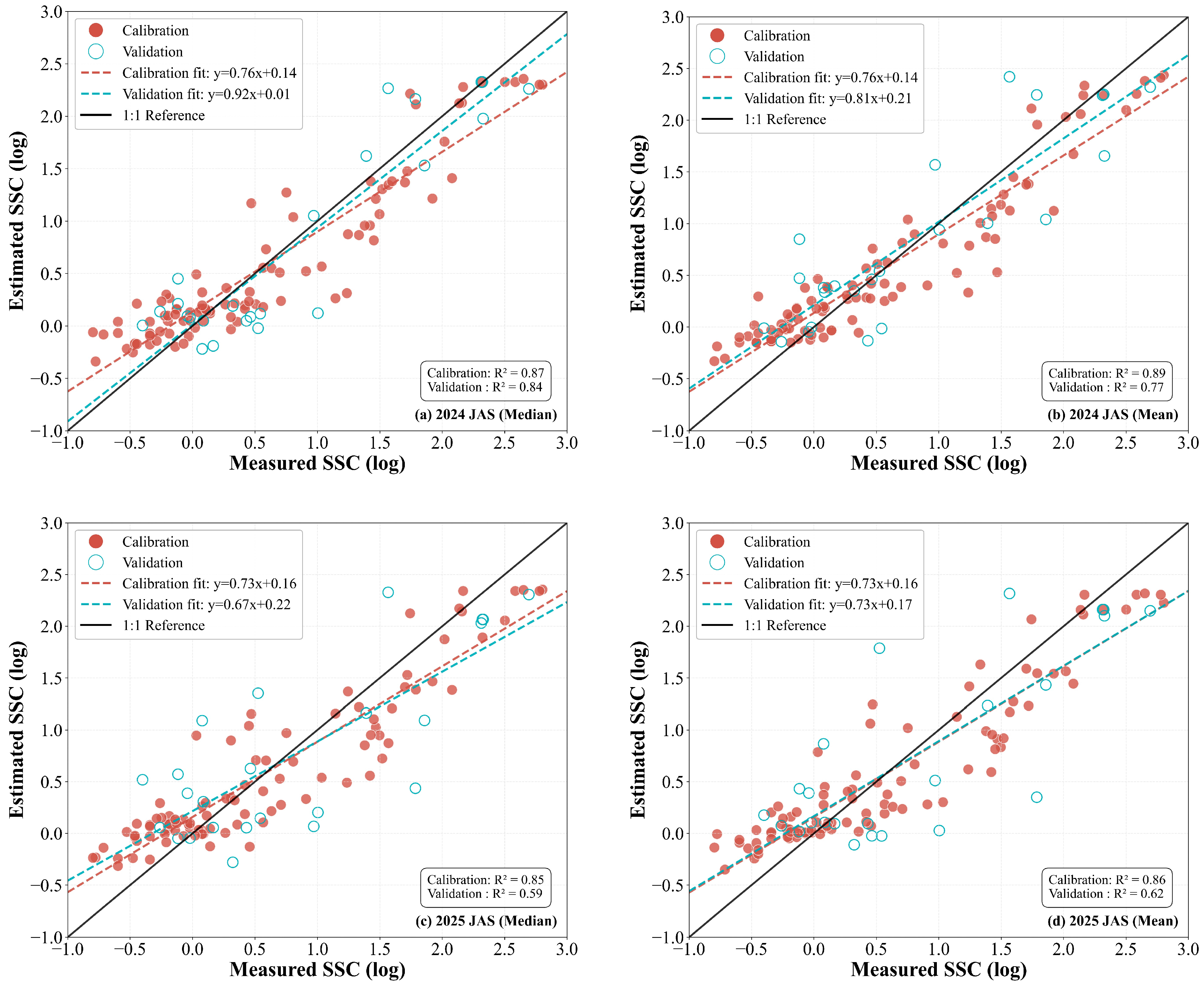
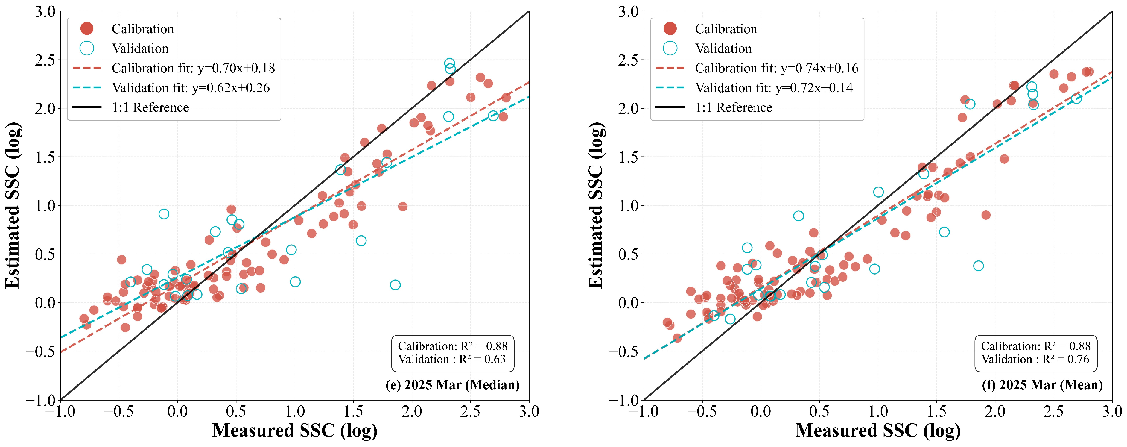
SSC prediction models were developed using the LightGBM machine learning algorithm, incorporating two distinct synthesis strategies: the 2024 JAS (July–August–September) legacy period and the 2025 JAS stress period, alongside concurrent data from March 2025. Evaluation of the training and testing sets through the distribution of data points relative to the 1:1 regression line (y = x) provided a direct visualization of systematic bias and generalization capability. The results revealed that the LightGBM model based on the 2024 JAS median synthesis strategy performed best, achieving the highest R2 of 0.84 on the test set (Figure 8a), which slightly outperformed the mean synthesis strategy (Figure 8b). The 2024 JAS median composite outperformed the mean composite, achieving a higher R2 (0.84 vs. 0.77) and a lower RMSE on the validation set. The statistical gain from the median synthesis strategy stems from its inherent resistance to stochastic outliers, such as residual cloud shadows and transient surface moisture variations, which tend to skew the spectral mean. Consequently, the prior-season median composite provides a more robust input for the model, effectively enhancing the stability and accuracy of the inversion results. When log-transformed soil salinity values were below 0.5, data points for all strategy models were distributed above the 1:1 line, indicating a significant overestimation of salinity in mildly salinized soils. Among all evaluated approaches, the 2024 JAS synthesis strategy yielded the optimal fitting results (Figure 8a). The fitting accuracy of the 2025 JAS synthesis strategy was lower than that of the 2024 JAS strategy, suggesting that salinization legacy effects contribute more significantly to model performance than salinization lag characteristics (Figure 8a–d). Comparisons with the March 2025 concurrent inversion results (Figure 8e,f) demonstrate that the integration of characteristic indices from the previous season significantly enhances the monitoring accuracy of soil salinity.
Figure 8.
Scatter plots of estimated versus observed values for models based on different time-window composition strategies. (a,b) are scatter plots of fitted values for the models based on the 3-month JAS (July-September) window using median and mean composite strategies, respectively, for 2024; (c,d) are scatter plots of fitted values for the models based on the 3-month JAS window using median and mean composite strategies, respectively, for 2025; (e,f) are scatter plots of fitted values for the models based on the 1-month March window using median and mean composite strategies, respectively, for 2025.
3.5. Correlations with In Situ, Legacy, and Stress-Period Features Based on the Optimal Median Strategy
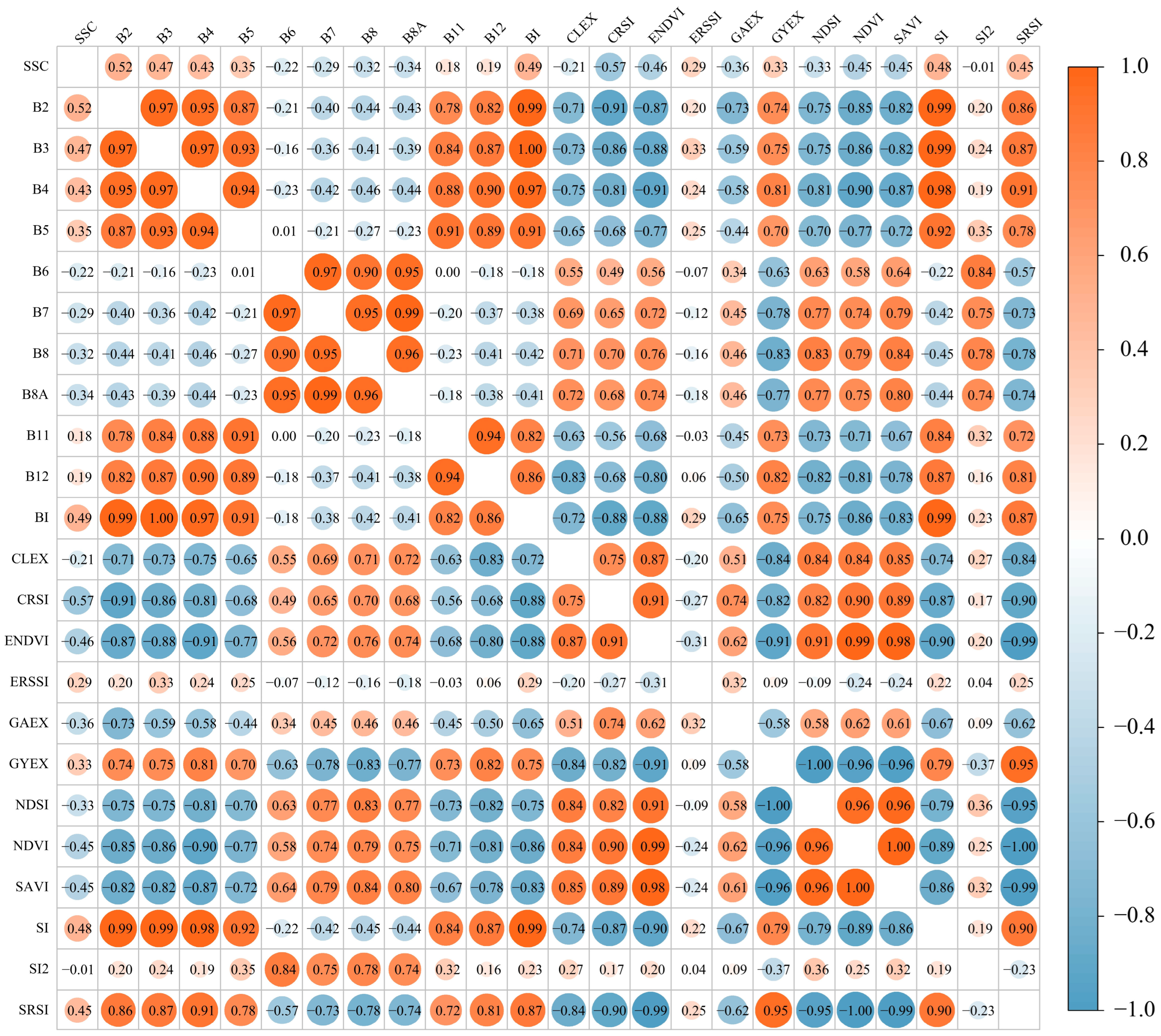
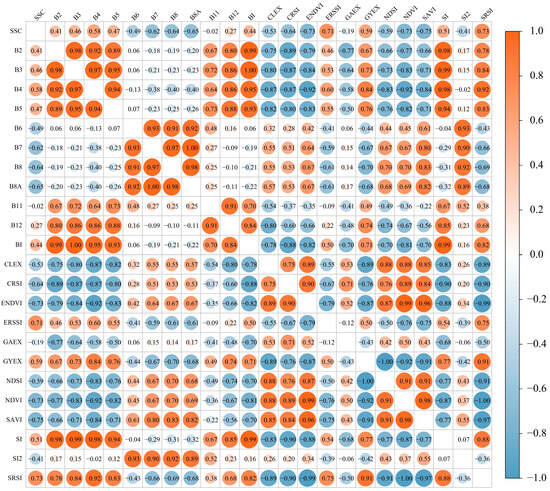
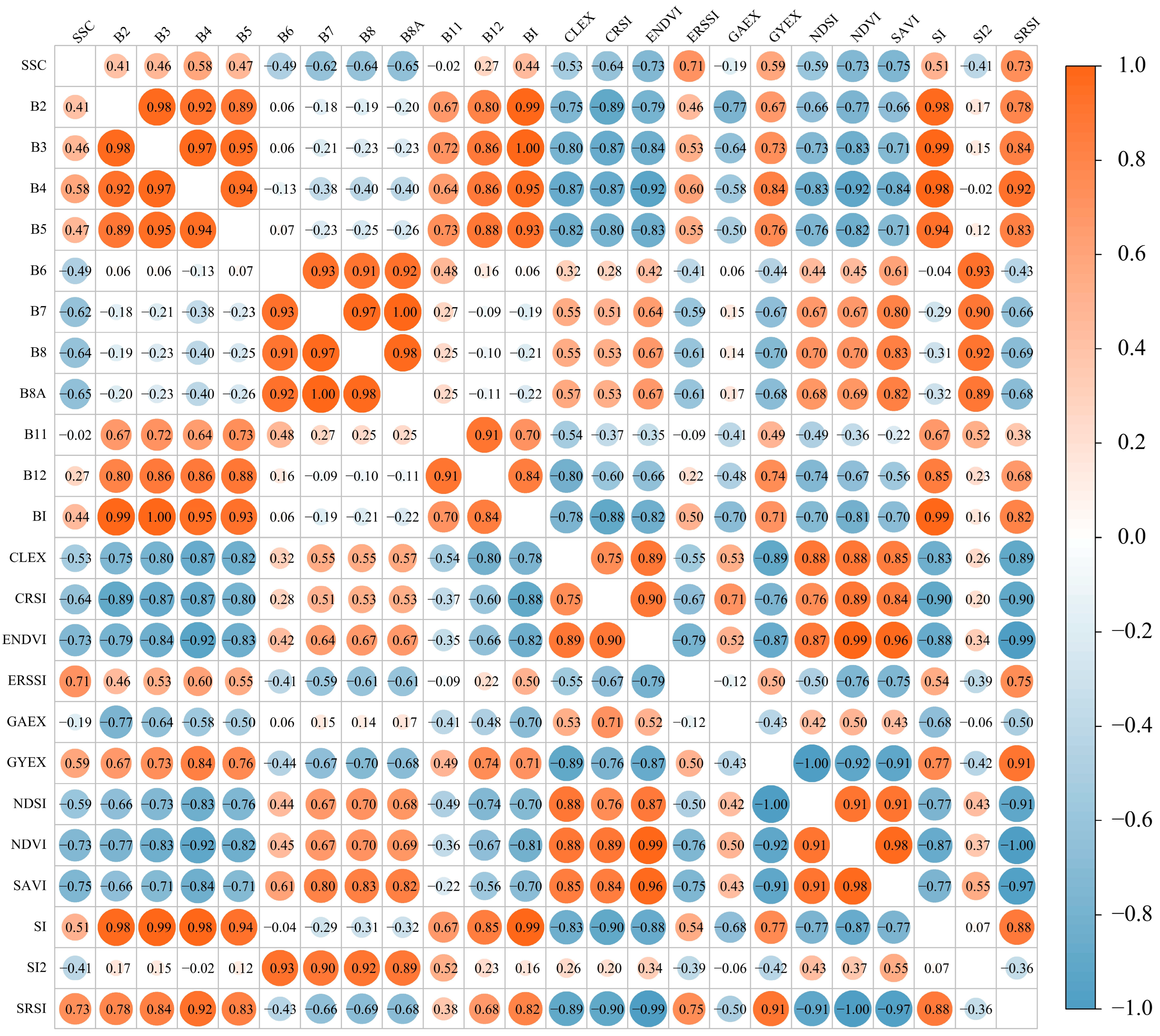
Based on the three optimal time-window, a correlation analysis was conducted between SSC and 23 raw spectral bands as well as derived remote sensing indices (Figure 9, Figure A3 and Figure A4).
Figure 9.
Correlation between legacy period soil salinity and spectral features.
The results indicated that for the 2024 JAS period, a significant negative correlation was exhibited between SSC and multiple composite vegetation indices (including CRSI, ENDVI, ERSSI, NDVI, SAVI, and SRSI) (Figure 9). Notably, vegetation-related single-band and multi-band indices significantly outperformed salinity indices and other single-band indices. This suggests a strong association between the vegetation information of the preceding year and the top SSC in the following spring. Among these, the highest correlation was observed with SRSI. Regions characterized by vigorous summer vegetation growth and complex canopy structures were associated with lower risks of soil salinization in the subsequent spring, effectively demonstrating the feasibility of predicting soil salinity in the following spring using remote sensing indices of vegetation stress from the growing season. During the March 2025 period, vegetation coverage is typically low. Consequently, spectral information primarily reflects the physicochemical properties of bare soil. A significant positive correlation was observed between SSC and visible light bands (B2, B3, B4, and BI), with correlation coefficients ranging from 0.43 to 0.52; the highest correlation was found with B2. Significant correlations were also noted with specific salinity indices (SI, SRSI), which may be attributed to variations in soil surface brightness, color, and roughness induced by salinity. Although plant growth is affected by soil salinity through osmotic stress—thereby altering reflectance characteristics in the red and near-infrared regions and resulting in negative correlations with vegetation indices such as CRSI and NDVI—vegetation in temperate zones has not yet fully regreened in March. As this period represents the early growing season, a substantial spectral contribution to mixed pixels is made by the soil background, thereby rendering indices sensitive to soil properties significantly correlated (Figure A3). Regarding the 2025 JAS period, significant differences were observed in the correlations between SSC and various remote sensing indices. Sites with higher spring SSC exhibited higher absolute index values in summer imagery. This may be attributed to the intense evaporation from high salinity soils during the arid summer, leading to the formation of salt crystals or crusts on the surface, which in turn enhances spectral reflectance. Furthermore, soils with high spring salinity possess a diminished capacity to support vegetation growth in summer. A significant negative correlation (with R ranging from −0.68 to −0.74) was demonstrated between SSC and indices such as NDVI, SAVI, and ENDVI. This reveals the inhibitory effect of salt stress on vegetation growth during the growing season (Figure A4).
3.6. Spatial Distribution Pattern of Soil Salinity
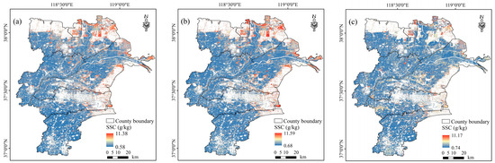
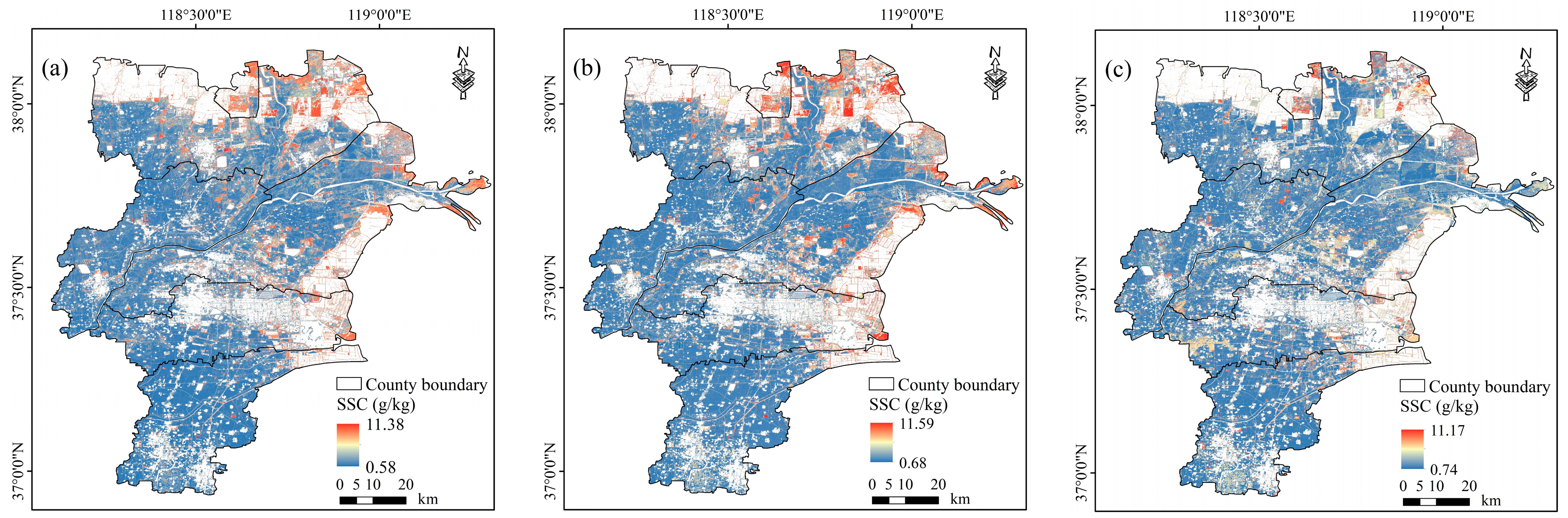
Figure 10 illustrates the spatial distribution of soil salinity derived from model inversion based on the median compositing strategy across the three optimal time windows: the legacy feature period, the stress feature period, and the concurrent period. Overall, consistent spatial distribution trends were exhibited by the compositing strategies across different time windows. High-salinity areas were primarily located in the northern and eastern coastal regions of the study area, whereas low-salinity areas were mainly concentrated in the southern irrigation districts. However, significant differences in salinity gradients and patch structures were revealed by the inversion results from different time windows.
Figure 10.
Spatial distribution of soil salinity derived from models based on the median composite strategy across different time windows. (a) Based on the feature set from JAS 2024. (b) Based on the feature set from JAS 2025 and (c) Based on the feature set from Mar 2025.
Figure 10a presents the spatial distribution of soil salinity derived from imagery data of July–September 2024, with a salinity range between 0.58 and 11.38 g/kg. Figure 10b depicts the results based on July–September 2025, similar to the 2024 results, the salinity ranged from 0.68 to 11.59 g/kg. Compared with the two summer maps, although a salinity range of 0.74–11.17 g/kg was maintained in the concurrent period inversion (Figure 10c), the proportion of pixels with high values was low, indicating that soil salinity was underestimated. The integration of vegetation features from the preceding growing season and the current growing season resulted in more natural spatial transitions. The distribution of high-salinity areas was coherent and consistent with the regional topography and the genesis of coastal saline lands, thereby demonstrating optimal spatial consistency.
4. Discussion
4.1. Optimal Window and Composition Strategy for Predicting Soil Salinity
This study identified the optimal temporal window and compositing strategy for soil salinity inversion by integrating multi-temporal satellite data across distinct growing seasons with advanced machine learning architectures. We explored the varying efficacies of satellite imagery from the preceding growing season, the current season, and the concurrent sampling period, while systematically evaluating the impact of different compositing methods on model robustness. In the context of soil salinity monitoring, median compositing effectively suppresses spectral outliers, whereas the minimum (Min) compositing strategy often lacks representativeness. Specifically, the Min strategy disproportionately emphasizes dark features, such as bare organic soil or shadows, which can mask the spectral signatures of saline soils that typically exhibit high reflectance [34]. The spectral manifestations of soil salinity are most pronounced under specific phenological stages or hydro-pedological conditions [35,36,37]. Given that the study area is an intensive agricultural zone, the optimal predictive window may not necessarily align with the actual sampling month due to the confounding effects of farming activities [38]. To rigorously evaluate temporal effectiveness, we tested 1-month and 3-month rolling compositing windows from March to October for both the preceding and current years, thereby facilitating a more robust capture of spatiotemporal salinity dynamics. Our results demonstrate that the period from July to September of the preceding year, which incorporates “legacy” vegetation signals, constitutes the optimal window for salinity estimation—a finding that aligns with the observations of Shi [39]. This was followed by concurrent modeling results, whose relatively lower performance may stem from soil moisture interference caused by spring freeze–thaw cycles or snowmelt, which effectively dampens the spectral response of salinity. Since precisely matching sampling dates with cloud-free image acquisition remains a logistical challenge, the use of composite imagery significantly enhances model applicability in practical scenarios [40]. Ultimately, these findings offer novel insights into the predictability of soil salinity prior to the onset of spring canopy closure.
Analysis indicates that the 1-month and 3-month temporal windows during the preceding summer consistently outperformed those from the concurrent growing season. This phenomenon is likely attributable to localized agricultural practices within the North China Plain, where the Winter Wheat–Summer Maize rotation predominates. During the peak growing season, the homogeneous canopy allows for the capture of robust spectral signatures induced by salinity-mediated vegetation stress [41]. In contrast, spring irrigation and reclamation measures typically trigger the transient leaching or redistribution of salts. Experimental data have demonstrated that post-irrigation, soil salinity across numerous plots decreases significantly, leading to a partial alleviation of vegetation stress. This shift in the vegetation-salinity dynamic relative to the preceding season effectively attenuates the sensitivity of the spectral response [42,43]. Findings from both the preceding year and the concurrent period underscore the primacy of spectral signatures related to environmental stressors. The strong negative correlation between prior-season vegetation indices and soil salinity proved to be a more effective predictor. This mechanism likely hinges on the capacity of the preceding summer window to capture salinity-induced stress within a relatively homogeneous and fully developed canopy. Here, vegetation growth status and stress levels serve as indirect proxies for the pedogenic background, integrating the authentic saline-alkali status under stable cropping and irrigation regimes [44]. Furthermore, summer evapotranspiration facilitates salt accumulation in the surface layer—a distribution pattern that exhibits significant temporal persistence. This confirms the feasibility of predicting subsequent spring salinity using legacy signals from the prior growing season. Before canopy closure, top-soil salinity is more intimately coupled with soil attributes and sensitive spectral bands. In these temperate regions, where vegetation has not yet fully regreened, the soil background provides a substantial spectral contribution to mixed pixels, rendering soil-sensitive indices highly significant [45,46,47]. Finally, concurrent agronomic interventions often mask visible salinity effects, thereby weakening the salinity-spectral coupling in vegetation [43,48]. These factors collectively elucidate the superior predictive stability of models anchored in the peak growing season of the preceding year.
Recent findings indicate that Solar-Induced Chlorophyll Fluorescence (SIF) data during the Asian summer exhibit the highest sensitivity in assessing agricultural soil salinity. SIF provides a near-real-time proxy for plant biochemistry and physiology [49,50], directly reflecting the immediate impacts of environmental stressors. Consequently, vegetation spectral information serves as a pivotal indicator for determining soil salinity levels. Salt stress typically triggers a reduction in chlorophyll content and structural leaf alterations, and as salinity intensifies, this inhibitory effect is clearly mirrored in the spectral signatures [51,52]. Thus, soil salinization can be monitored indirectly by analyzing indices of vegetation stress. Furthermore, salinity diminishes leaf water potential, thereby impairing water transport efficiency and inducing osmotic stress. This leads to an insufficient water supply for photosynthesis, triggering stomatal closure and a subsequent decline in chlorophyll concentration. Prolonged foliar dehydration culminates in plasmolysis and heightened cellular permeability [53,54]. These foliar alterations manifest as structural changes in the canopy, resulting in increased reflectance at water absorption wavelengths and decreased reflectance indicative of modified pigment content and cellular integrity [55]. Empirical research extensively supports the use of salinity-oriented indices—such as CRSI, ERSSI, ENDVI, and associated VI–SI combinations—as significant and sensitive indicators of vegetation salt stress and broader soil-vegetation salinization [22,56,57]. By integrating vegetation stress information, researchers can more accurately capture soil salinity dynamics and enhance monitoring precision, providing a critical observation window for the early warning of salinization.
The theoretical significance of utilizing legacy signals hinges on the biological integration effect, where vegetation serves as a continuous biosensor of soil stress over time. From an application perspective, this method facilitates the transition from reactive monitoring to proactive early warning. By identifying high-risk salinized zones months before spring sowing, agricultural managers can optimize leaching schedules and select appropriate salt-tolerant genotypes, thereby enhancing the resilience of coastal agriculture under a changing climate.
4.2. Limitations and Future Research
Despite the promising results obtained in this study, several specific limitations must be acknowledged to ensure a rigorous interpretation. First, regarding sensor and temporal constraints, the acquisition of high-quality remote sensing data is frequently hindered by cloud cover and aerosols. While ‘legacy signals’ from vegetation offer a novel proxy, the lack of direct soil observations during peak canopy closure may limit the characterization of rapid salinity fluctuations. Second, the current soil-depth focus is restricted to the 0–20 cm layer. While this depth is critical for crop growth, the vertical movement of salts across the entire soil profile, especially the influence of shallow groundwater—was not explicitly modeled, which may introduce uncertainties in areas with complex water-table dynamics. Third, anthropogenic factors in agricultural irrigation districts, such as specific leaching measures and complex cropping patterns, pose challenges for model generalization. Finally, the regional transferability of the proposed composition strategy framework requires further validation in other arid or semi-arid coastal ecosystems. Future research should aim to integrate multi-source data (e.g., SIF or microwave remote sensing) with explicit physical mechanisms to elucidate soil water-salt movement from a microscopic perspective, thereby enhancing both the generalizability and physical basis of soil salinity inversion.
5. Conclusions
This study leveraged Sentinel-2 imagery and implemented multi-temporal compositing strategies via the Google Earth Engine (GEE) platform. We evaluated the potential for monitoring soil salinity prior to the onset of spring canopy closure and determined the optimal temporal windows and spectral features for assessing spring salinity in the Yellow River Delta irrigation district. These findings offer novel insights into the early warning and proactive management of soil salinization. Specifically, at a single-month scale, the median compositing strategy during August and September emerged as the optimal window for assessment; simultaneously, the July–September (JAS) interval was identified as the superior three-month temporal window. Regarding spectral characteristics, vegetation stress indicators exhibited a robust correlation with subsequent spring soil salinity, contributing most significantly to the predictive accuracy of the model. This research demonstrates that precise early-season salinity forecasting can be achieved by utilizing prior-season feature imagery. Ultimately, this work establishes a comprehensive framework for soil salinity early warning, providing a scientific foundation for future efforts to optimize feature selection and temporal window identification in coastal ecosystems.
Author Contributions
Conceptualization, J.Z., T.L., L.H. and W.F.; data curation, Z.Z. and L.H.; funding acquisition, T.L., W.F. and L.H.; methodology, J.Z., L.H. and M.W.; visualization, J.Z., H.L. and D.H.; writing—original draft, J.Z.; Writing—reviewing and editing, J.Z., T.L. and W.F. All authors have read and agreed to the published version of the manuscript.
Funding
This research was funded by the State Key Laboratory of Nutrient Use and Management (No. GZ202011), the Research Startup Grant (No. CXGC2025G03), the National Center of Technology Innovation for Comprehensive Utilization of Saline-Alkali Land “Challenge-Based Project” (NO. GYJ2023002), the Natural Science Foundation of Shandong Province (NO. ZR2024QD029), the National Natural Science Foundation of China (NO. 42401079) and the Qingdao Natural Science Foundation (NO. 24-4-4-zrjj-45-jch).
Data Availability Statement
The data presented in this study are available on request from the corresponding author.
Conflicts of Interest
The authors declare no conflicts of interest.
Appendix A
Figure A1.
2D scatter density plots of SWIR for different composition strategies at the 3-month scale.
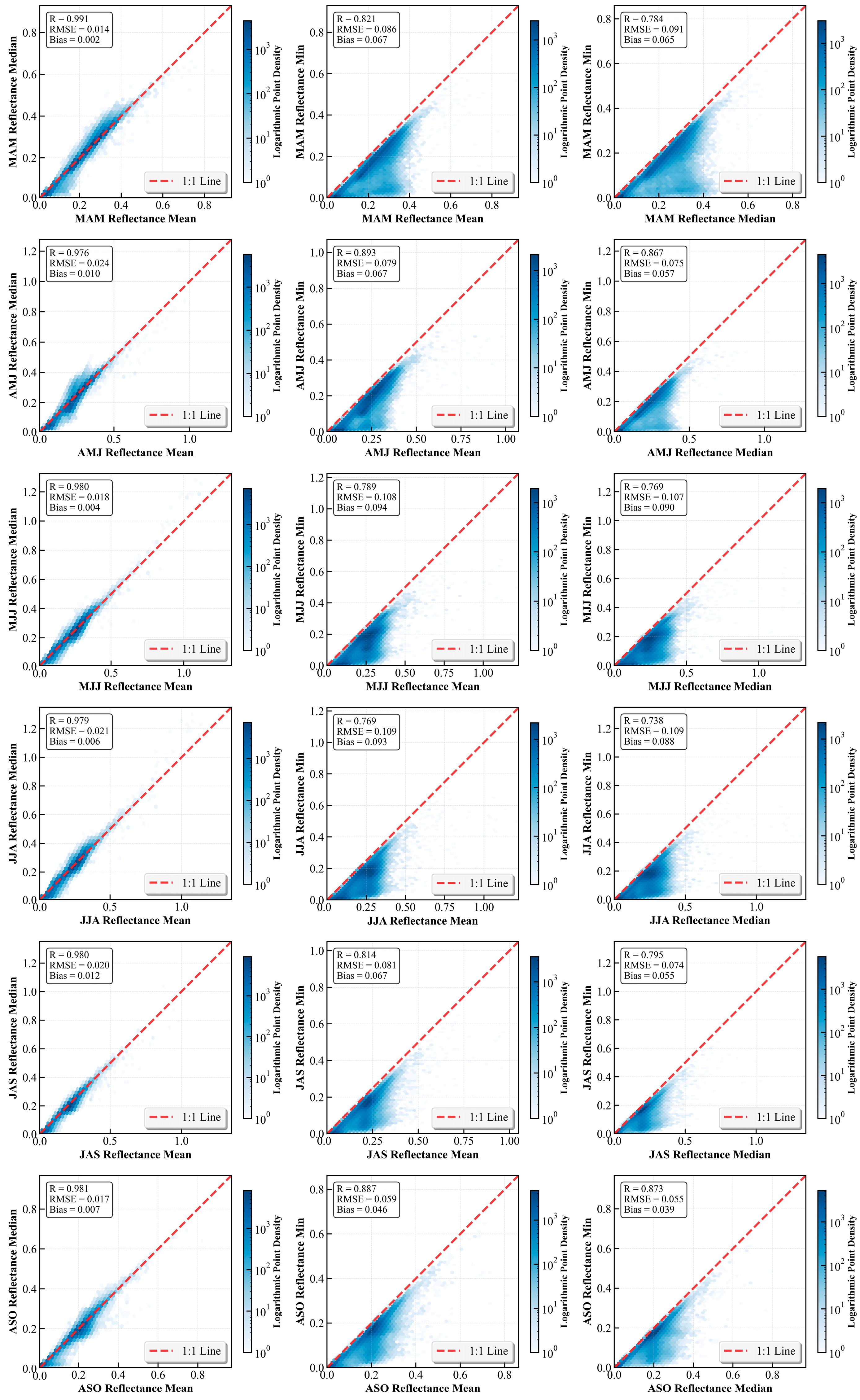
Figure A2.
Evaluation of R2, RMSE, and RPIQ for models using 3-month composition strategies; (a–c,g–i,m–o) training set, (d–f,j–l,p–r) validation set.
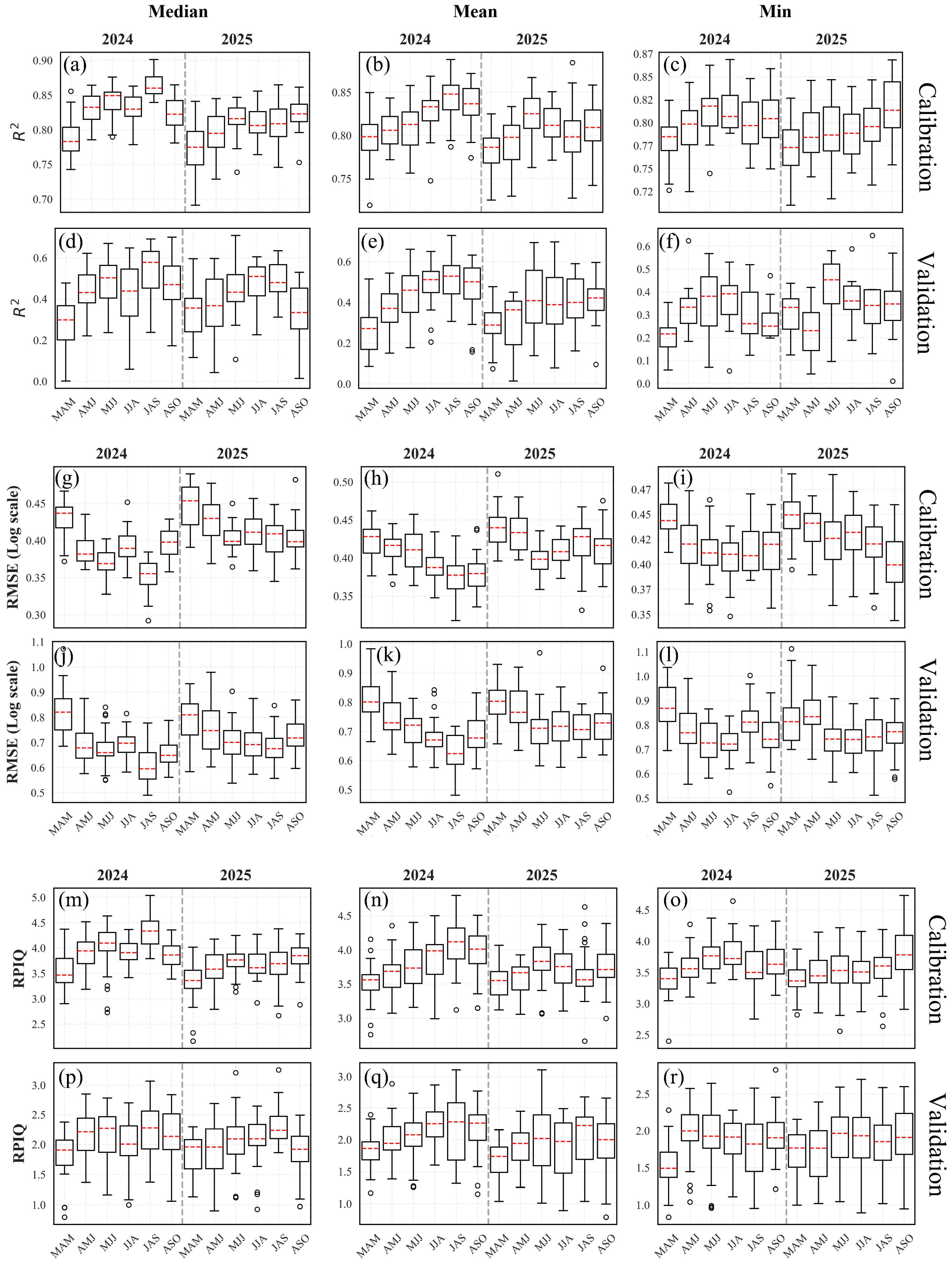
Figure A3.
Correlation between stress period soil salinity and spectral features.
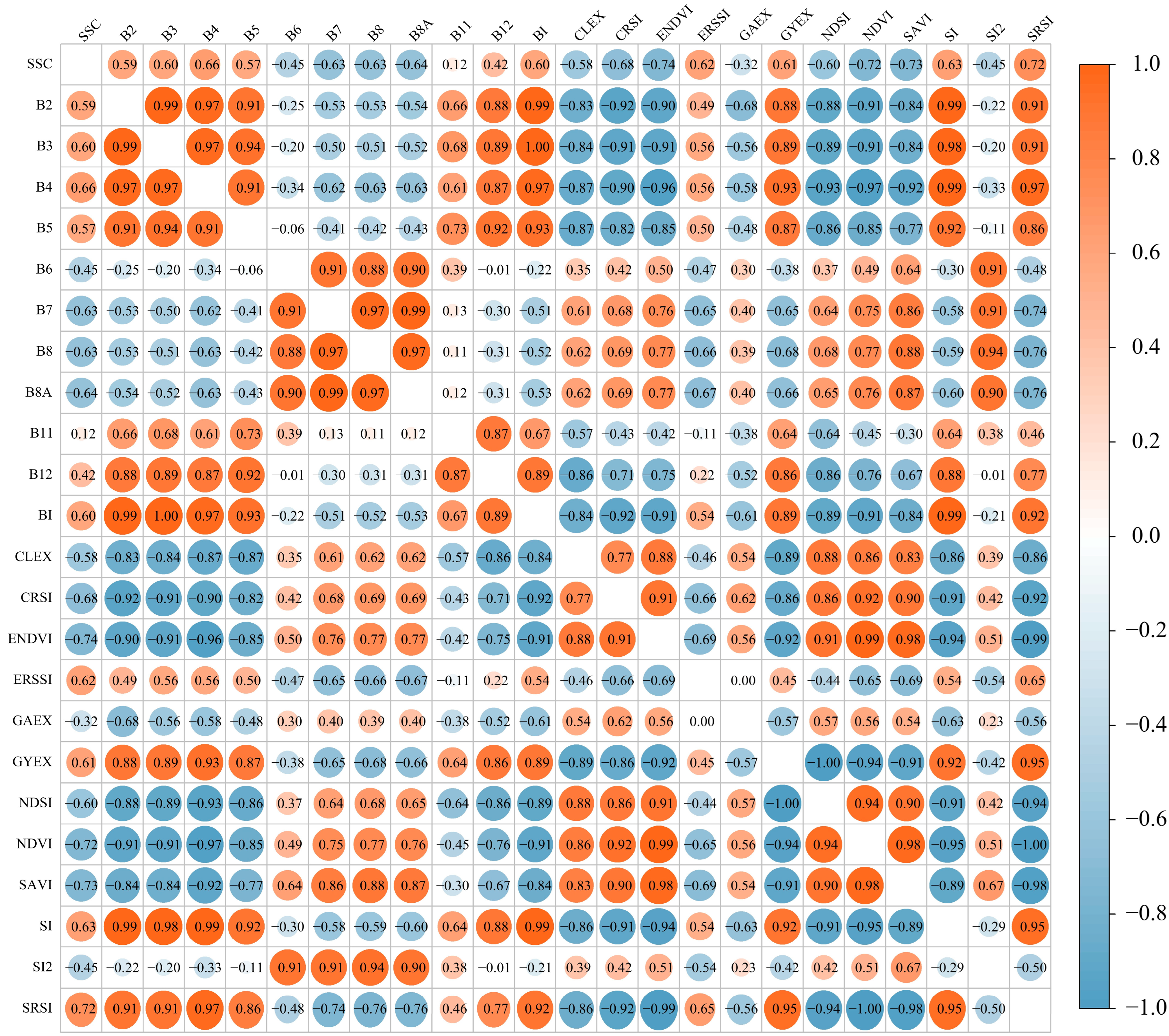
Figure A4.
Correlation between in situ soil salinity and spectral features.
References
- Luo, Z.; Deng, M.; Tang, M.; Liu, R.; Feng, S.; Zhang, C.; Zheng, Z. Estimating Soil Profile Salinity under Vegetation Cover Based on UAV Multi-Source Remote Sensing. Sci. Rep. 2025, 15, 2713. [Google Scholar] [CrossRef] [Scilit]
- Jia, P.; Zhang, J.; He, W.; Yuan, D.; Hu, Y.; Zamanian, K.; Jia, K.; Zhao, X. Inversion of Different Cultivated Soil Types’ Salinity Using Hyperspectral Data and Machine Learning. Remote Sens. 2022, 14, 5639. [Google Scholar] [CrossRef] [Scilit]
- Chen, H.; Zhao, G.; Li, Y.; Wang, D.; Ma, Y. Monitoring the Seasonal Dynamics of Soil Salinization in the Yellow River Delta of China Using Landsat Data. Nat. Hazards Earth Syst. Sci. 2019, 19, 1499–1508. [Google Scholar] [CrossRef] [Scilit]
- Wang, J.D.; Sun, Z.G.; Yang, T.; Zhu, K.Y.; Shao, C.X.; Peng, J.B.; Wang, W.Y.; Gao, Y.N.; Yue, H.Y. A Remote Sensing Method for Retrieving Soil Salinity Based on CYGNSS: Taking the Yellow River Delta as an Example. Natl. Remote Sens. Bull. 2023, 27, 351–362. [Google Scholar] [CrossRef] [Scilit]
- Song, Y.; Gao, M.; Wang, Z.; Gong, T.; Chen, W. Spatio–Temporal Variability Characteristics of Coastal Soil Salinization and Its Driving Factors Detection. Water 2022, 14, 3326. [Google Scholar] [CrossRef] [Scilit]
- Sahbeni, G.; Ngabire, M.; Musyimi, P.; Székely, B. Challenges and Opportunities in Remote Sensing for Soil Salinization Mapping and Monitoring: A Review. Remote Sens. 2023, 15, 2540. [Google Scholar] [CrossRef] [Scilit]
- Wang, F.; Han, L.; Liu, L.; Bai, C.; Ao, J.; Hu, H.; Li, R.; Li, X.; Guo, X.; Wei, Y. Advancements and Perspective in the Quantitative Assessment of Soil Salinity Utilizing Remote Sensing and Machine Learning Algorithms: A Review. Remote Sens. 2024, 16, 4812. [Google Scholar] [CrossRef] [Scilit]
- Chen, H.; Wu, J.; Xu, C. Monitoring Soil Salinity Classes through Remote Sensing-Based Ensemble Learning Concept: Considering Scale Effects. Remote Sens. 2024, 16, 642. [Google Scholar] [CrossRef] [Scilit]
- Bandak, S.; Movahedi-Naeini, S.A.; Mehri, S.; Lotfata, A. A Longitudinal Analysis of Soil Salinity Changes Using Remotely Sensed Imageries. Sci. Rep. 2024, 14, 10383. [Google Scholar] [CrossRef] [Scilit]
- Yu, X.; Chang, C.; Song, J.; Zhuge, Y.; Wang, A. Precise Monitoring of Soil Salinity in China’s Yellow River Delta Using UAV-Borne Multispectral Imagery and a Soil Salinity Retrieval Index. Sensors 2022, 22, 546. [Google Scholar] [CrossRef] [Scilit]
- Colpaert, A. Satellite and UAV Platforms, Remote Sensing for Geographic Information Systems. Sensors 2022, 22, 4564. [Google Scholar] [CrossRef] [Scilit]
- Wang, J.; Ding, J.; Ge, X.; Peng, J.; Hu, Z. Monitoring Soil Salinization Based on Remote Sensing and Proximal Soil Sensing: Progress and Perspective. Natl. Remote Sens. Bull. 2023, 28, 2187–2208. [Google Scholar] [CrossRef] [Scilit]
- Zarei, A.; Hasanlou, M.; Mahdianpari, M. A Comparison of Machine Learning Models for Soil Salinity Estimation Using Multi-Spectral Earth Observation Data. ISPRS Ann. Photogramm. Remote Sens. Spat. Inf. Sci. 2021, V-3–2021, 257–263. [Google Scholar] [CrossRef] [Scilit]
- Jia, P.; Zhang, J.; He, W.; Hu, Y.; Zeng, R.; Zamanian, K.; Jia, K.; Zhao, X. Combination of Hyperspectral and Machine Learning to Invert Soil Electrical Conductivity. Remote Sens. 2022, 14, 2602. [Google Scholar] [CrossRef] [Scilit]
- Wang, N.; Xue, J.; Peng, J.; Biswas, A.; He, Y.; Shi, Z. Integrating Remote Sensing and Landscape Characteristics to Estimate Soil Salinity Using Machine Learning Methods: A Case Study from Southern Xinjiang, China. Remote Sens. 2020, 12, 4118. [Google Scholar] [CrossRef] [Scilit]
- Ding, Q.; Huang, H.; Zhang, J.; Wang, Y.; Jia, K. Estimating Soil Moisture and Organic Matter Contents in Salt-Affected Farmlands Using Hyperspectral Remote Sensing Machine Learning. Res. Sq. 2024; preprint. [CrossRef] [Scilit]
- Zhou, M.; Li, Y. Digital Mapping and Scenario Prediction of Soil Salinity in Coastal Lands Based on Multi-Source Data Combined with Machine Learning Algorithms. Remote Sens. 2024, 16, 2681. [Google Scholar] [CrossRef] [Scilit]
- Zhou, M.; Li, Y. Spatial Distribution and Source Identification of Potentially Toxic Elements in Yellow River Delta Soils, China: An Interpretable Machine-Learning Approach. Sci. Total Environ. 2024, 912, 169092. [Google Scholar] [CrossRef] [Scilit] [PubMed]
- Ouzemou, J.-E.; Laamrani, A.; El Battay, A.; Whalen, J.K. Predicting Soil Salinity Based on Soil/Water Extracts in a Semi-Arid Region of Morocco. Soil Syst. 2025, 9, 3. [Google Scholar] [CrossRef] [Scilit]
- Dinamarca, D.I.; Galleguillos, M.; Seguel, O.; Faúndez Urbina, C. CLSoilMaps: A National Soil Gridded Database of Physical and Hydraulic Soil Properties for Chile. Sci. Data 2023, 10, 630. [Google Scholar] [CrossRef] [Scilit]
- Zhang, C.; Yi, P.; Liu, Y.; Ma, L.; Hu, W.; Wu, J. Thin Cloud Correction Method for Visible Remote Sensing Images Using a Spectral Transformation Scheme. GISci. Remote Sens. 2023, 60, 2196133. [Google Scholar] [CrossRef] [Scilit]
- Wang, N.; Peng, J.; Chen, S.; Huang, J.; Li, H.; Biswas, A.; He, Y.; Shi, Z. Improving Remote Sensing of Salinity on Topsoil with Crop Residues Using Novel Indices of Optical and Microwave Bands. Geoderma 2022, 422, 115935. [Google Scholar] [CrossRef] [Scilit]
- Scudiero, E.; Skaggs, T.H.; Corwin, D.L. Regional Scale Soil Salinity Evaluation Using Landsat 7, Western San Joaquin Valley, California, USA. Geoderma Reg. 2014, 2–3, 82–90. [Google Scholar] [CrossRef] [Scilit]
- Wang, F.; Ding, J.; Wu, M. Remote Sensing Monitoring Models of Soil Salinization Based on NDVI-SI Feature Space. Trans. Chin. Soc. Agric. Eng. 2010, 26, 168–173. [Google Scholar]
- Traba, J.; Gómez-Catasús, J.; Barrero, A.; Bustillo-de la Rosa, D.; Zurdo, J.; Hervás, I.; Pérez-Granados, C.; García de la Morena, E.L.; Santamaría, A.; Reverter, M. Comparative Assessment of Satellite- and Drone-Based Vegetation Indices to Predict Arthropod Biomass in Shrub-Steppes. Ecol. Appl. 2022, 32, e2707. [Google Scholar] [CrossRef] [Scilit] [PubMed]
- Mokarram, M.; Hojjati, M.; Roshan, G.; Negahban, S. Modeling the Behavior of Vegetation Indices in the Salt Dome of Korsia in North-East of Darab, Fars, Iran. Model. Earth Syst. Environ. 2015, 1, 27. [Google Scholar] [CrossRef] [Scilit]
- Liu, H.; Guo, B.; Yang, X.; Zhao, J.; Li, M.; Huo, Y.; Wang, J. High Spatiotemporal Resolution Vegetation Index Time Series Can Facilitate Enhanced Remote Sensing Monitoring of Soil Salinization. Plant Soil 2024, 510, 305–327. [Google Scholar] [CrossRef] [Scilit]
- Khan, N.M.; Rastoskuev, V.V.; Sato, Y.; Shiozawa, S. Assessment of Hydrosaline Land Degradation by Using a Simple Approach of Remote Sensing Indicators. Agric. Water Manag. 2005, 77, 96–109. [Google Scholar] [CrossRef] [Scilit]
- Taghizadeh-Mehrjardi, R.; Minasny, B.; Sarmadian, F.; Malone, B.P. Digital Mapping of Soil Salinity in Ardakan Region, Central Iran. Geoderma 2014, 213, 15–28. [Google Scholar] [CrossRef] [Scilit]
- Nicolas, H.; Walter, C. Detecting Salinity Hazards within a Semiarid Context by Means of Combining Soil and Remote-Sensing Data. Geoderma 2006, 134, 217–230. [Google Scholar] [CrossRef] [Scilit]
- Jia, P.; Zhang, J.; Liang, Y.; Zhang, S.; Jia, K.; Zhao, X. The Inversion of Arid-Coastal Cultivated Soil Salinity Using Explainable Machine Learning and Sentinel-2. Ecol. Indic. 2024, 166, 112364. [Google Scholar] [CrossRef] [Scilit]
- Jiang, Z.; Hao, Z.; Ding, J.; Miao, Z.; Zhang, Y.; Alimu, A.; Jin, X.; Cheng, H.; Ma, W. Weighted Variable Optimization-Based Method for Estimating Soil Salinity Using Multi-Source Remote Sensing Data: A Case Study in the Weiku Oasis, Xinjiang, China. Remote Sens. 2024, 16, 3145. [Google Scholar] [CrossRef] [Scilit]
- Wang, W.; Dong, L.; Ma, C.; Wei, L.; Xu, F.; Feng, J. Experimental Investigation of Ground Radiation on Dielectric and Brightness Temperature of Soil Moisture and Soil Salinity. Sensors 2020, 20, 2806. [Google Scholar] [CrossRef] [Scilit] [PubMed]
- Wang, D.; Yang, H.; Qian, H.; Gao, L.; Li, C.; Xin, J.; Tan, Y.; Wang, Y.; Li, Z. Minimizing Vegetation Influence on Soil Salinity Mapping with Novel Bare Soil Pixels from Multi-Temporal Images. Geoderma 2023, 439, 116697. [Google Scholar] [CrossRef] [Scilit]
- Zhu, K.; Sun, Z.; Zhao, F.; Yang, T.; Tian, Z.; Lai, J.; Zhu, W.; Long, B. Relating Hyperspectral Vegetation Indices with Soil Salinity at Different Depths for the Diagnosis of Winter Wheat Salt Stress. Remote Sens. 2021, 13, 250. [Google Scholar] [CrossRef] [Scilit]
- Sui, Y.; Jiang, R.; Liu, Y.; Zhang, X.; Lin, N.; Zheng, X.; Li, B.; Yu, H. Predicting the Spatial Distribution of Soil Salinity Based on Multi-Temporal Multispectral Images and Environmental Covariates. Comput. Electron. Agric. 2025, 231, 109970. [Google Scholar] [CrossRef] [Scilit]
- Farifteh, J.; Meer, F.; Meijde, M.; Atzberger, C. Spectral Characteristics of Salt-Affected Soils: A Laboratory Experiment. Geoderma 2008, 145, 196–206. [Google Scholar] [CrossRef] [Scilit]
- Ma, S.; He, B.; Ge, X.; Luo, X. Spatial Prediction of Soil Salinity Based on the Google Earth Engine Platform with Multitemporal Synthetic Remote Sensing Images. Ecol. Inform. 2023, 75, 102111. [Google Scholar] [CrossRef] [Scilit]
- Shi, S.; Wang, N.; Chen, S.; Hu, B.; Peng, J.; Shi, Z. Digital Mapping of Soil Salinity with Time-Windows Features Optimization and Ensemble Learning Model. Ecol. Inform. 2025, 85, 102982. [Google Scholar] [CrossRef] [Scilit]
- Whitney, K.; Scudiero, E.; El-Askary, H.; Skaggs, T.; Allali, M.; Corwin, D. Validating the Use of MODIS Time Series for Salinity Assessment over Agricultural Soils in California, USA. Ecol. Indic. 2018, 93, 889–898. [Google Scholar] [CrossRef] [Scilit]
- Xiong, J.; Ge, X.; Ding, J.; Wang, J.; Zhang, Z.; Zhu, C.; Han, L.; Wang, J. Optimal Time-Window for Assessing Soil Salinity via Sentinel-2 Multitemporal Synthetic Data in the Arid Agricultural Regions of China. Ecol. Indic. 2025, 176, 113642. [Google Scholar] [CrossRef] [Scilit]
- Yang, N.; Yang, S.; Cui, W.; Zhang, Z.; Zhang, J.; Chen, J.; Ma, Y.; Lao, C.; Song, Z.; Chen, Y. Effect of Spring Irrigation on Soil Salinity Monitoring with UAV-Borne Multispectral Sensor. Int. J. Remote Sens. 2021, 42, 8952–8978. [Google Scholar] [CrossRef] [Scilit]
- Du, R.; Chen, J.; Zhang, Z.; Chen, Y.; He, Y.; Yin, H. Simultaneous Estimation of Surface Soil Moisture and Salinity during Irrigation with the Moisture-Salinity-Dependent Spectral Response Model. Agric. Water Manag. 2022, 265, 107538. [Google Scholar] [CrossRef] [Scilit]
- El-Ramady, H.; Prokisch, J.; Mansour, H.; Bayoumi, Y.A.; Shalaby, T.A.; Veres, S.; Brevik, E.C. Review of Crop Response to Soil Salinity Stress: Possible Approaches from Leaching to Nano-Management. Soil. Syst. 2024, 8, 11. [Google Scholar] [CrossRef] [Scilit]
- Nguyen, K.-A.; Liou, Y.-A.; Tran, H.-P.; Hoang, P.-P.; Nguyen, T.-H. Soil Salinity Assessment by Using Near-Infrared Channel and Vegetation Soil Salinity Index Derived from Landsat 8 OLI Data: A Case Study in the Tra Vinh Province, Mekong Delta, Vietnam. Prog. Earth Planet. Sci. 2020, 7, 1. [Google Scholar] [CrossRef] [Scilit]
- Wu, D.; Jia, K.; Zhang, X.; Zhang, J.; El-Hamid, H.A. Remote Sensing Inversion for Simulation of Soil Salinization Based on Hyperspectral Data and Ground Analysis in Yinchuan, China. Nat. Resour. Res. 2021, 30, 4641–4656. [Google Scholar] [CrossRef] [Scilit]
- Barreto, A.; Neto, M.F.; Oliveira, R.; Moreira, L.C.J.; Medeiros, J.; Sá, F. Comparative Analysis of Spectral Indexes for Soil Salinity Mapping in Irrigated Areas in a Semi-Arid Region, Brazil. J. Arid. Environ. 2023, 209, 104888. [Google Scholar] [CrossRef] [Scilit]
- Wang, X.; Ainiwaer, M.; Maimaitituersun, A.; Zhang, J.; Subi, X. Prediction of Soil Salinization in Arid Regions during Wet and Dry Seasons Based on Spectro-Polarimetric Features and Machine Learning. Land Degrad. Dev. 2025, 36, 4290–4303. [Google Scholar] [CrossRef] [Scilit]
- Du, R.; Xiang, Y.; Chen, J.; Lu, X.; Wu, Y.; He, Y.; Xiang, R.; Zhang, Z.; Chen, Y. Potential of Solar-Induced Chlorophyll Fluorescence (SIF) to Access Long-Term Dynamics of Soil Salinity Using OCO-2 Satellite Data and Machine Learning Method. Geoderma 2024, 444, 116855. [Google Scholar] [CrossRef] [Scilit]
- Wang, K.; Zhu, J.; Xu, X.; Li, T.; Wang, X.; Warner, T.; Cheng, T.; Zhu, Y.; Cao, W.; Yao, X.; et al. Quantitative Monitoring of Salt Stress in Rice with Solar-Induced Chlorophyll Fluorescence. Eur. J. Agron. 2023, 150, 126954. [Google Scholar] [CrossRef] [Scilit]
- Negrão, S.; Schmöckel, S.; Tester, M. Evaluating Physiological Responses of Plants to Salinity Stress. Ann. Bot. 2016, 119, 1–11. [Google Scholar] [CrossRef] [Scilit] [PubMed]
- Zhang, T.-T.; Zeng, S.; Gao, Y.; Ouyang, Z.; Li, B.; Fang, C.; Zhao, B. Using Hyperspectral Vegetation Indices as a Proxy to Monitor Soil Salinity. Ecol. Indic. 2010, 11, 1552–1562. [Google Scholar] [CrossRef] [Scilit]
- Mao, P.; Lin, Q.; Pang, Y.; Wang, K.; Ni, R.; Han, X.; Cao, B. Eco-Physiological Response Mechanism of Tamarix Chinensis to Soil Water Changes in Coastal Wetlands of the Yellow River Delta. Front. Mar. Sci. 2023, 10, 1231928. [Google Scholar] [CrossRef] [Scilit]
- Ma, Y.; Liu, W.; Qiao, Y.; Qiao, W.; Yang, H.; Zhong, Y.; Yang, H.; Wang, H.; Li, Y.; Dong, B.; et al. Effects of Soil Salinity on Foxtail Millet Osmoregulation, Grain Yield, and Soil Water Utilization under Varying Water Conditions. Agric. Water Manag. 2023, 284, 108354. [Google Scholar] [CrossRef] [Scilit]
- Gu, H.; Yin, G.; Yang, Y.; Verger, A.; Descals, A.; Filella, I.; Zeng, Y.; Hao, D.; Xie, Q.; Li, X.; et al. Satellite-Detected Contrasting Responses of Canopy Structure and Leaf Physiology to Drought. IEEE J. Sel. Top. Appl. Earth Obs. Remote Sens. 2023, 16, 2427–2436. [Google Scholar] [CrossRef] [Scilit]
- Guo, B.; Han, B.; Yang, F.; Fan, Y.; Jiang, L.; Chen, S.; Yang, W.; Gong, R.; Liang, T. Salinization Information Extraction Model Based on VI–SI Feature Space Combinations in the Yellow River Delta Based on Landsat 8 OLI Image. Geomat. Nat. Hazards Risk 2019, 10, 1863–1878. [Google Scholar] [CrossRef] [Scilit]
- Ramos, T.; Castanheira, N.; Oliveira, A.; Paz, A.; Darouich, H.; Simionesei, L.; Farzamian, M.; Gonçalves, M. Soil Salinity Assessment Using Vegetation Indices Derived from Sentinel-2 Multispectral Data. Application to Lezíria Grande, Portugal. Agric. Water Manag. 2020, 241, 106387. [Google Scholar] [CrossRef] [Scilit]

Disclaimer/Publisher’s Note: The statements, opinions and data contained in all publications are solely those of the individual author(s) and contributor(s) and not of MDPI and/or the editor(s). MDPI and/or the editor(s) disclaim responsibility for any injury to people or property resulting from any ideas, methods, instructions or products referred to in the content. |
© 2026 by the authors. Licensee MDPI, Basel, Switzerland. This article is an open access article distributed under the terms and conditions of the Creative Commons Attribution (CC BY) license.