


Highlights
What are the main findings?
- Bayesian kriging (BK) densifies sparse SST and chlorophyll-a observations into 30–500 m coastal fields with calibrated uncertainty (posterior mean and 95% prediction intervals). Repeated 80/20 cross validation shows consistent out-of-sample skill and interval coverage close to the nominal 95%.
- Independent grid-to-grid benchmarking against satellite products (MUR SST for Algarve, Landsat-8 OC3 chlorophyll for La Spezia) is performed on the native prediction grids, with satellite fields used strictly for external validation (i.e., not used as model inputs in the baseline experiments). A matched sparsity baseline using ordinary kriging (OK) complements this evaluation, enabling a direct BK–OK comparison that reports both point prediction skill and uncertainty calibration.
What is the implication of the main finding?
- The workflow yields reproducible, georeferenced maps and uncertainty layers that are directly usable for coastal monitoring and risk-aware decision making.
- The workflow is predictor-free and variable-agnostic in formulation (applicable to scalar coastal fields without auxiliary covariates), demonstrated here on SST and Chl across two coastal pilots. Boader generalization to other regimes is a natural next step when suitable data are available.
Abstract
In many environmental applications, high-quality measurements are too sparse to resolve the small-scale patterns required for process understanding and management. We investigate a Bayesian kriging (BK) framework that densifies sparse coastal observations into high-resolution gridded fields with calibrated uncertainty. Two pilot sites are considered: (i) sea surface temperature (SST) in the Algarve (Portugal), where point measurements (~10 km spacing) are reconstructed on a 500 m grid, and (ii) chlorophyll (Chl) in the La Spezia embayment (Italy), where in situ supported fields are reconstructed at 30 m. The variogram parameters are treated as random variables with weakly informative priors and inferred via MCMC, so that both measurement noise and structural (variogram) uncertainty are propagated to predictions, yielding posterior means and 95% prediction intervals per grid cell. Independent repeated 80/20 cross validation demonstrates robust out-of-sample skill in both sites. For Algarve, the BK maps recover fine-scale thermal structure while preserving defensible uncertainty under severe sparsity. For La Spezia, the same framework resolves estuarine gradients at 30 m. Credible intervals widen away from observations yet remain sufficiently narrow elsewhere to guide interpretation. Satellite products are used strictly for validation on a common grid (MUR SST at 1 km resampled to 500 m, Landsat OC3 Chl at 30 m), confirming spatial fidelity and clarifying seasonal differences. Overall, the approach produces uncertainty-aware, high-resolution coastal fields from heterogeneous, sparse records, supporting reproducible EO analyses and risk-aware coastal monitoring.
1. Introduction
Environmental monitoring often relies on sparse spatial datasets, where high-quality measurements cover only limited locations. As a result, extensive gaps in coverage hinder our ability to resolve fine-scale patterns that matter for process understanding and management [1]. Such gaps can bias representations of key processes and propagate uncertainty downstream into modeling and decision making. Spatial densification seeks to transform sparse measurements into continuous, high-resolution fields, thereby providing more informative geophysical surfaces for climate diagnostics, resource management and hazard assessment. Satellite remote sensing has partly alleviated sparsity by offering broad coverage at increasingly fine resolution, yet coastal zones remain challenging due to clouds, adjacency effects, sunglint and complex optics. Moreover, satellite scenes are intermittent and may be asynchronous with in situ sampling [2]. Integrating remote sensing with ground measurements is a promising strategy to fill gaps and capture complex spatial patterns, but effective fusion and uncertainty quantification require robust geostatistical methods [3]. Classical ordinary kriging uses spatial autocorrelation (via variograms) to estimate values at unsampled locations [4]. Under sparsity, however, standard kriging typically relies on a single empirically fitted variogram whose parameters (range, sill, nugget) are treated as known [5]. In practice, these parameters are estimated from limited data and entail non-negligible uncertainty; ignoring them leads to underestimated prediction intervals and overconfident maps. What is needed is a densification approach that: (i) preserves geostatistical interpretability; (ii) propagates parameter and process uncertainty into predictions; and (iii) remains independent of external predictors during fitting so that any satellite-based comparison is truly out-of-sample.
High-resolution Earth Observation products (e.g., Landsat/Sentinel optical imagery and GHRSST Level-4 SST analyses) substantially improve spatial coverage, yet coastal waters remain challenging due to clouds, adjacency effects, sunglint, and optically complex conditions. Our objective is not to replace satellite products, but to reconstruct gap-free, measurement-anchored fields from sparse in situ observations with rigorously quantified uncertainty. This predictor-free design also preserves a genuinely independent satellite benchmark, because EO products are used strictly for evaluation and never enter the Bayesian likelihood or priors.
BK addresses these needs by treating variogram parameters as random variables with priors that are updated by the data to posteriors [6,7]. This hierarchical formulation explicitly propagates both measurement noise and structural uncertainty to the predictive surface, producing posterior means together with 95% prediction intervals for every grid node. When prior knowledge exists (e.g., expected correlation ranges or instrument error models), it can be encoded transparently; otherwise, weakly informative priors can be used. In all cases, the outcome is a probabilistic densification surface that supports risk-aware interpretation, not just a single best guess map. Related variants, empirical Bayesian kriging (EBK), regression/co-kriging and other semi-Bayesian schemes attempt to average over multiple semivariogram realizations or to inject ancillary predictors, often improving over a single fixed variogram while remaining less explicit about prior structure and full posterior predictive inference [8,9,10]. Machine learning algorithms (e.g., random forests, SVMs, neural networks) can be powerful when rich covariates are available, but typically require extensive training data, careful tuning and add-on procedures for uncertainty. Moreover, they may not explicitly handle spatial autocorrelation or local non-stationarity without specialized extensions [11,12,13,14,15]. By contrast, Bayesian geostatistics retains a well understood Gaussian process foundation and produces principled uncertainty estimates, particularly valuable when data are scarce and prior information must be leveraged.
In this study, the BK framework is empirically validated only in nearshore/coastal waters (an open-margin shelf and a semi-enclosed embayment). Although the statistical formulation is generally predictor-free and variable-agnostic in formulation (i.e., applicable to scalar fields without auxiliary covariates), its predictive performance and uncertainty calibration in open ocean settings or in strongly non-stationary regimes are not assessed here and should be examined in future work. This framing is intentional: The two case studies are presented as pilot demonstrations of the workflow and uncertainty calibration under sparse in situ support, rather than as a comprehensive multi-region benchmark.
These considerations are directly relevant to Earth Observation (EO): Many remote sensing products already involve densification or fusion steps (e.g., gap-free land surface temperature, downscaling of coarse satellite retrievals to finer grids, integration of satellite products with sparse ground stations for air quality mapping), where rigorous per-pixel uncertainty is essential for downstream use [16,17,18,19,20]. Coastal and estuarine waters, in particular, exhibit sharp sub-kilometer gradients driven by tides, wind-driven upwelling/relaxation, river plumes, bathymetry and harbor dynamics. Both SST and Chl vary on short spatial and temporal scales and can be strongly modulated by turbidity and optical complexity near the coast [21]. Satellite products partly mitigate data sparsity, but in coastal zones they still suffer from clouds/adjacency effects, sunglint and shoreline contamination, while reanalysis fields are often too smooth to resolve nearshore fronts and small plumes [22]. Region-specific studies highlight these challenges: Along the Algarve (S. Portugal), the Iberian upwelling system produces strong, rapidly evolving SST fronts, with coastal jets and filaments at sub-kilometer scales. In the semi-enclosed Gulf of La Spezia (Ligurian Sea), complex circulation, variable bathymetry, port activity and intermittent freshwater inputs create fine-scale heterogeneity and intermittent Chl blooms [23]. Previous coastal mapping efforts (SST/Chl) in comparable European embayments often rely on kriging/co-kriging, EBK or ML workflows, with limited treatment of spatial leakage and predictive interval calibration under extreme sparsity [24].
Against this background, we adopt a fully Bayesian, covariate-free kriging framework to densify sparse coastal observations while quantifying uncertainty. We address a single question: Can we reconstruct high-resolution coastal fields from sparse in situ data alone, with defensible uncertainty, and verify spatial fidelity independently? We operationalize this question in two contrasting pilot sites: first, sea surface temperature (SST) in the Algarve (Portugal), where point measurements (typical spacing ~10 km) are reconstructed on a 500 m analysis grid matched to shoreline geometry; second, chlorophyll (Chl) in the semi-enclosed La Spezia embayment (Italy), where measurements are reconstructed at 30 m to resolve estuarine gradients and nearshore heterogeneity. In both sites, the modeling equation remains predictor-free; satellite products are used only for out-of-sample benchmarking on a common grid (MUR SST at 1 km resampled to 500 m in Algarve, and Landsat OC3 Chl at 30 m in La Spezia), avoiding leakage between fitting and evaluation [16,17,18,19,20,21,22,23,24].
Our validation protocol has two complementary parts. First, we perform repeated 80/20 cross validation with strictly held-out test sets, reporting medians and interquartile ranges of RMSE/MAE/Bias together with the empirical coverage of the nominal 95% prediction intervals, thus quantifying out-of-sample skill and uncertainty calibration under the actual sampling density [4,5,6,7]. Second, we conduct grid-to-grid comparisons against the independent satellite products at matched resolution, optionally applying a GAM calibration to the satellite field (for evaluation only, see Section 4.5) to reduce cross-sensor scale bias. This clarifies how absolute agreement varies by season and local water optics while leaving the Bayesian fit itself unaffected [16,17,18,19,20]. Methodologically, our contribution is threefold. (i) We provide a variable-agnostic Bayesian reconstruction that yields posterior means and intervals at 30 and 500 m from sparse in situ data, without incorporating external predictors [6,7,8,9]. (ii) We formalize a transparent, reproducible procedure, MCMC diagnostics, repeated 80/20 CV, interval width maps and independent grid-to-grid benchmarking, that turns kriged grids into traceable data products [5,6,7]. (iii) We articulate application boundaries that matter in practice: approximate stationarity within the analysis window, and sufficient spatial spread of in situ points relative to the inferred correlation range and caution in the presence of sharp fronts or rapidly evolving coastal optics (where absolute agreement with raw satellite scenes can degrade even when out-of-sample CV remains adequate) [21,22,23,24]. In this way, the analysis remains interpretable within a geostatistical framework [25].
The remainder of the paper is organized as follows: Section 2 outlines the Bayesian formulation and the validation protocol. Section 3 introduces the two coastal sites and data. Section 4 describes the BK workflow and experimental design. Section 5 presents the results. Section 6 discusses implications, limitations and boundaries of use. Section 7 concludes.
2. Theoretical Background
We treat each target variable as a spatial random field and model the insitu observations within each period using a Gaussian process (GP) framework [26] with a constant mean and stationary covariance.
Let y(s) denote the observed value at location s. We adopt the common “signal + noise” formulation in which y(s) = β0 + w(s) + ε(s), where β0 is an intercept, w(s) is a zero mean GP capturing spatial dependence [27], and ε(s)~N(0, τ2) is an independent nugget. Ordinary kriging (OK) yields best linear unbiased predictions when the covariance is treated as fixed, whereas Bayesian kriging (BK) additionally accounts for uncertainty in the covariance parameters.
Spatial dependence in w(s) is represented with a Matern covariance, parameterized by partial sill σ2, range φ, and smoothness ν. The nugget τ2 captures measurement error and unresolved sub-grid variability. The Matern family is flexible (spanning exponential to Gaussian-like behavior) and is widely used in environmental and oceanographic spatial modeling [28].
In BK, we place prior distributions on the model parameters θ = {β0, σ2, τ2, φ, ν} and infer their posterior distribution conditional on the observations. Compared with OK, BK propagates parameter uncertainty into predictions, which is central for uncertainty-aware spatial densification.
Priors are chosen to be weakly informative to stabilize inference under sparse sampling while remaining broad on the data scale; the exact hyperparameters used for each case study are summarized in Table A1 (Appendix A.2).
Posterior inference is performed via Metropolis within Gibbs Markov chain Monte Carlo (MCMC). Posterior samples are then propagated to the target grid to obtain the posterior predictive mean, standard deviation, and 95% prediction intervals.
These predictive summaries support both interpolation (densification) and uncertainty quantification, and they are evaluated using repeated holdout cross validation and independent satellite comparisons (Section 4).
Formally, combining the likelihood and priors via Bayes’s theorem yields the joint posterior p(β0, θ, w|y) ∝ p(y|β0, θ, w) p(w|θ) p(β0) p(θ), which we approximate through MCMC sampling.
In practice, we report both point predictions (posterior mean) and calibrated uncertainty products (posterior standard deviation and 95% prediction intervals) to support risk-aware analysis.
The same BK workflow is applied to SST in the Algarve (500 m grid) and chlorophyll in the Gulf of La Spezia (native 30 m Landsat grid), demonstrating transfer across variables and resolutions.
p(Z(s0)|Z) = ∫ p(Z(s0)|β, θ, Z)… p(β, θ|Z) dβ dθ
Section 4 details the implementation choices, prediction grids, and validation protocol used in this study.
3. Case Studies
3.1. Pilot Site Selection
Two coastal pilot sites were selected to demonstrate the proposed Bayesian spatial densification under distinct spatial and environmental conditions. The first site, in the Algarve region of southern Portugal, represents an open-ocean-influenced coastal system at the transition between the eastern North Atlantic and the western Mediterranean, where wind-driven circulation, intermittent upwelling and coastal jets generate energetic, rapidly evolving SST structures. The second site, the Gulf of La Spezia (Ligurian Sea, NW Italy), is a semi-enclosed system where riverine and nearshore mixing govern sharp biogeochemical gradients, including intermittent Chl blooms. These contrasting regimes were chosen to test one coherent research question, whether a fully Bayesian geostatistical framework can reconstruct high-resolution coastal fields from sparse data with calibrated uncertainty and to illustrate the method’s applicability across different physical and biogeochemical settings. In both sites, satellite products are used exclusively for independent validation on a matched grid, not as predictors in the kriging equation, so that benchmarking against EO is genuinely out-of-sample.
3.2. The Algarve Pilot Site
The Algarve pilot area lies along the southern Iberian margin, where Atlantic and Mediterranean waters interact. The study domain spans approximately 2900 km2 of coastal ocean. The target variable for densification is SST, reconstructed on a 500 m analysis grid (chosen to resolve fine-scale thermal structure while remaining well posed under the available sampling). The kriging input consisted exclusively of SST measurements: (i) irregularly spaced shipborne transects sampling a continuous path across the domain, which leave large portions of the area unobserved (derived from Copernicus Marine Service in situ observations, access via the Copernicus Marine Data Store) and (ii) a fixed coastal buoy near Faro (≈36°54′N, 7°54′W), providing a high-accuracy SST time series to anchor the in situ dataset (Faro buoy SST observations were retrieved from the Portuguese Hydrographic Institute portal). All point measurements were co-registered in a common WGS-84 reference prior to modeling.
For contextual comparison and independent benchmarking (held out from model fitting; not used as BK inputs), we used:
- ➢
- ODYSSEA/CMEMS Level-4 SST reanalysis at ~0.10° (~9–10 km) native spacing, used only to illustrate the coarse scale background structure over the domain.
- ➢
- GHRSST MUR (Multi-scale Ultra-high-resolution) Level-4 SST analysis (nominal ~1 km), resampled to 500 m to match the BK grid and used strictly for independent grid-to-grid comparison.
The BK model is response only: It is trained exclusively on the in situ SST point measurements and delivers posterior means and 95% prediction intervals on the 500 m analysis grid. For Algarve SST, the 500 m spacing is a pragmatic compromise: It is good enough to represent kilometer-scale coastal fronts and upwelling filaments, while remaining numerically well posed under sparse support and computationally tractable; it also enables straightforward comparison with widely used ~1 km gridded SST products (e.g., MUR) via simple resampling. The CMEMS/ODYSSEA and MUR products are withheld from model fitting and are used only for out-of-sample evaluation of absolute agreement and scale consistency (Section 4).
3.3. The La Spezia Pilot Site
The La Spezia site encompasses the Magra River estuary and its surrounding coastal waters along the Ligurian Sea in NW Italy. This area is characterized by complex land–sea interactions, where estuarine discharge and coastal ocean processes intersect. The Magra River delivers freshwater and nutrient loads into the coastal zone, creating a buoyant plume that mixes with saline waters. Wind-driven circulation and tidal exchanges further influence the dispersion of this plume. These estuarine and coastal mixing processes lead to strong gradients in water parameters, particularly in chlorophyll, a proxy for phytoplankton biomass and coastal eutrophication. Elevated Chl levels often develop near the river mouth due to nutrient enrichment, while offshore waters remain lower in productivity, resulting in sharp spatial contrasts. The study area covers the immediate coastal zone around the river outlet and adjacent sea (order of a few tens of square kilometers, roughly 4–5 km across). This environmental complexity and relevance to water quality make La Spezia an important case for testing the densification of biogeochemical data.
For the La Spezia coastal region, we analyzed two characteristic periods: March, when river-borne nutrients can trigger intense blooms, and September, when concentrations are typically reduced following the summer period. The target variable for densification was Chl, reconstructed on a 30 m analysis grid to (i) preserve the native Landsat pixel support for comparisons and (ii) resolve strong sub-kilometer nearshore gradients (e.g., plume/embayment structure) that are common in small coastal basins. The kriging input consisted exclusively of in situ measurements within the study area. All point measurements were harmonized in a common spatial reference and screened for plausibility prior to modeling (unit/CRS harmonization, temporal focus, shoreline mask). Because the available in situ support is sparse and unevenly distributed (with fewer observations close to the shoreline), large parts of the 4–5 km coastal swath remain unobserved, motivating a probabilistic spatial reconstruction that explicitly carries uncertainty (see also the Data Availability Statement for the origin of the data).
To assess spatial fidelity, satellite products were used only for independent validation on a matched grid. Specifically, Landsat OC3 Chl at 30 m was prepared for the two dates, co-registered to the densified grid and used for grid-to-grid benchmarking. A simple GAM calibration of the satellite field to initial measurements scale was employed to reduce cross-sensor scale bias (see Section 4.5). The spatial patterns observed in the densified Chl maps are consistent with known environmental gradients and plume behavior in the area [29,30,31], with credible intervals widening away from observations yet remaining sufficiently narrow elsewhere to support interpretation and water quality screening.
3.4. Densification Grid
For each study site, we defined a target prediction grid that balances the resolution needed to capture small-scale variability with computational tractability and a consistent shoreline mask. For the Algarve SST case, we constructed a 500 m analysis grid covering the coastal area of interest (approximately 50 km × 58 km). This resolution is substantially finer than the ~9–10 km scale of the coarse background fields and is also finer than the along-track spacing of the in situ measurements. For the La Spezia Chl case, densification was carried out on a 30 m grid specifically designed to resolve nearshore gradients and the river plume structure. This 30 m grid was built in the local UTM projection for numerical stability and precise shoreline alignment. In both sites, grid nodes that fell on land (per the land/water mask) were excluded, so that predictions were generated only over the water domain.
The Bayesian kriging produces a probabilistic output on these grids. At each retained grid node, the model yields a posterior mean (see also Appendix A.1), a posterior standard deviation, and a 95% prediction interval (defined by the q2.5 and q97.5 quantiles). Satellite products used for validation were co-registered to the corresponding densified grids (for example, MUR SST was resampled to the 500 m grid for Algarve and Landsat OC3 Chl to the 30 m grid for La Spezia) to enable direct grid-to-grid comparisons without any modeling circularity. To make the evaluation design explicit, we first summarize the spatial sampling geometry at both pilot sites and indicate which gridded EO products are used strictly as external references (Figure 1).
Figure 1.
Spatial distribution of the in situ observations used as inputs to Bayesian kriging and the external gridded products used only for contextual comparison. (a) Algarve (Portugal): dashed teal line = shipborne SST transect; red circle = Faro buoy. The orange box indicates the study region. The regular 0.1° grid shown in green corresponds to an external Level−4 background field (ODYSSEA/CMEMS) and is displayed for context only. (b) La Spezia (Italy): in situ chlorophyll sampling locations. Any gridded EO/reanalysis products are used strictly for independent evaluation, not as predictors in the BK likelihood (see Section 3.2 and Section 3.3).
4. Model Specification, Implementation, and Evaluation Framework
4.1. Bayesian Kriging Formulation
We apply Bayesian kriging (BK) to spatially densify sparse in situ observations and to quantify predictive uncertainty. Figure 2 summarizes the workflow used for both pilot sites.
Figure 2.
The workflow of the methodology.
Briefly, the workflow is as follows. We (i) define an overlap safe prediction grid aligned with the evaluation product (Algarve: 500 m grid aligned to MUR; La Spezia: native 30 m Landsat grid masked to water and AOI). We then (ii) fit the Gaussian process model to the in situ observations and (iii) sample from the posterior via MCMC. Finally, we (iv) generate posterior predictive distributions on the grid (mean, SD, and 95% prediction intervals) and (v) assess skill via repeated 80/20 cross validation and independent satellite comparisons.
Model formation and assumptions.
We model the in situ response y(s) at location s as:
with with x(s) = 1 (intercept) and with β0 is a constant mean term at each site/period, w(s) is a zero mean Gaussian process (GP) capturing spatial dependence and ε(s)~N(0, τ2) is an independent nugget. Within each site and period, we assume second-order stationarity and isotropy after projecting coordinates to a metric CRS.
We use a Matern covariance for w(s), with parameters controlling variance (σ2), correlation range (φ), and smoothness (ν). The nugget τ2 represents measurement error and unresolved variability. This parameterization is used consistently across sites to enable comparable uncertainty summaries.
Rationale under sparsity. Although coastal dynamics are inherently non-stationary and anisotropic (e.g., across fronts or river plumes), we employ a stationary, isotropic Matern model as a parsimonious baseline. Given the extreme sparsity of the in situ sampling available in this study, fitting complex non-stationary or shoreline-aware covariance structures would require estimating significantly more hyperparameters, leading to potential overfitting and unstable convergence. By relying on a stationary formulation, we ensure model identifiability while allowing the Bayesian framework to propagate structural uncertainty. Consequently, we interpret the resulting high-resolution maps as probabilistic texture fields conditioned on sparse observations, and we rely on posterior predictive diagnostics to identify regions where fine-scale structure is weakly constrained.
Priors and likelihood.
Weakly informative priors for θ are described in Section 4.2 (hyperparameters in Table A1, Appendix A.2).
Bayesian update and MCMC.
Posterior inference is performed via Metropolis within Gibbs MCMC [32] using spBayes (Section 4.3), yielding samples of θ and the latent field.
Prediction grids and masking.
Posterior predictive summaries are computed on the target grid, including posterior mean (μ), standard deviation (SD), and 95% prediction intervals (q0.025–q0.975), which are mapped as uncertainty products.
Validation protocol.
Validation is carried out in two complementary ways: repeated holdout cross validation on the in situ data (Section 4.4) and independent comparisons against satellite products (Section 4.5).
Repeated 80/20 cross-validation with strictly held-out test sets is used (Table 1). We report medians for RMSE, MAE, Bias, and the empirical coverage of the nominal 95% prediction intervals at test points for Algarve (Table 2) and La Spezia (Table 3).
Table 1.
(a) Cross-validated accuracy metrics (medians across 20 repeated 80/20 CV runs for each dataset). Coverage95 is the fraction of held-out points within the 95% predictive interval. (b) BK vs. ordinary kriging (OK) under repeated 80/20 cross validation (in parentheses median (IQR) across 20 runs). RMSE, MAE, Bias and PI-width are reported in the units of the target variable (°C for SST; mg m−3 for Chl-a), Coverage95 is unitless. (c) Grid-to-grid benchmarking against satellite products on the native prediction grids (BK vs. OK). RMSE, MAE and Bias are reported in the units of the target variable (°C for SST; mg m−3 for Chl), n pixels is the number of valid overlapping pixels used in the comparison. (d) Dynamic feature diagnostics for grid-to-grid benchmarking against independent satellite products (BK vs. OK). Recomputes diagnostics on gradient defined subsets (“dynamic” vs. “other”) after reprojection/masking and thresholding of the reference field.
Table 2.
Algarve SST densification performance.
Table 3.
La Spezia chlorophyll densification results. (a) Repeated 80/20 CV performance (median held-out metrics for each month). (b) Independent comparison between the BK 30 m grid and Landsat-8 OC3 chlorophyll (30 m, same dates) using raw satellite values (uncalibrated). March 2024 had higher chlorophyll levels (and errors) than September 2024. Units: mg m−3 for all error metrics.
For each evaluation we report RMSE, MAE, bias, R2, 95% interval coverage, and interval width, enabling direct comparisons between BK and baseline interpolators under sparse sampling.
Performance summaries and model validation.
All processing is implemented in R and applied with the same pipeline across sites, with site-specific inputs and prediction grids. This supports reproducibility and facilitates transfer across variables.
Assumptions.
The following subsections provide the implementation details of the priors, MCMC settings [33,34,35], prediction, and evaluation protocol.
4.2. Priors and Parameterization
We assign weakly informative priors to the mean and covariance parameters to stabilize inference under sparse sampling while remaining broad on the data scale.
β0∼N(0, 106)
We use inverse gamma priors for the partial sill σ2 and nugget τ2, and uniform priors for the range φ and smoothness ν. Bounds for φ follow standard spatial statistics guidance and are linked to the empirical point spacing.
ϕ∼Unif(ϕmin, ϕmax) with bounds derived from the point geometry (e.g., nearest/farthest pair distances),
ν∼Unif(0.5, 2.5) to allow moderate to smooth behavior.
Under the GP assumption, the likelihood of the observations is multivariate normal N(μ, Σ(θ)) with θ = {β0, σ2, τ2, ϕ, ν}.
These priors are combined with the GP likelihood to obtain the joint posterior distribution. Inference and prediction are based on MCMC samples (Section 4.3).
Sensitivity checks indicated that the main results and uncertainty calibration are robust to reasonably widen the prior ranges; the final hyperparameter values are reported in Table A1 (Appendix A.2).
To keep the main methodological narrative concise, the case-specific prior hyperparameters (Algarve SST; La Spezia Chl) are summarized in Table A1 rather than being listed here.
4.3. MCMC Configuration
We fit the BK model using Metropolis within Gibbs MCMC via spBayes::spLM with a Matern covariance, sampling θ = {β0, σ2, τ2, φ, ν} together with the latent spatial process.
Proposal distributions are tuned in short pilot runs to achieve stable mixing and reasonable acceptance rates; detailed settings are provided in Table A2 (Appendix A.2).
Convergence and mixing are assessed using trace plots, effective sample size, and Geweke diagnostics (we report no meaningful deviations from stationarity when |z| < 2) in Table A3 (Appendix A.2).
Across both pilot sites, we ran MCMC chains on the order of 105 iterations. Burn-in and thinning were selected to yield stable posterior summaries. The exact iteration counts and thinning factors used in each case study are reported in Table A2.
Across both pilot sites, chains were run on the order of 105 iterations with burn-in and thinning chosen to yield stable posterior summaries; the exact iteration counts and thinning factors used in each case study are listed in Table A2.
This Bayesian workflow yields calibrated uncertainty products (e.g., interval coverage) that can be directly evaluated alongside point accuracy metrics.
All reported prediction maps are based on posterior predictive summaries; uncertainty maps are produced alongside mean fields for each period and variable.
To facilitate reviewer comparison, we additionally implement an ordinary kriging (OK) baseline using the same prediction grids and the same validation protocol (Section 4.6).
The next sections describe the cross validation design and the satellite comparison protocol used to quantify interpolation performance.
4.4. Cross Validation Design
We assess predictive accuracy and uncertainty calibration using repeated 80/20 cross validation (CV) with strictly held-out test sets. For each repetition r = 1, …, 20 a random 80/20 split is drawn from the measurement dataset. The model is fitted only on the 80% training subset and predictions are computed only at the 20% held-out points. No observation appears in both train and test within the same split. We use fixed seeds to ensure reproducibility and, whenever an alternative baseline is considered, we reuse the identical train/test masks across models.
Across the 20 repetitions, we computed the following metrics on each held-out test set and report their median across all repetitions: RMSE, MAE, Bias, Coverage95 (the empirical fraction of test observations falling within the nominal 95% posterior predictive interval) and PI-width (the median width of the 95% posterior predictive interval). Because the test sets are relatively small in each repetition, Coverage95 can only take certain discrete values (e.g., 1.00, 0.86, …). Therefore, we also report a pooled coverage (Table A4, Appendix A.2) calculated over all held-out points aggregated across the 20 runs. We emphasize that all error metrics are calculated using only the held-out test data, no in-sample residuals or training errors are included in any reported summary or table.
Use of posterior output for validation: The 80/20 protocol prevents train–test leakage by design and mirrors the real-world use case (predict at locations with no concurrent observations). To facilitate model evaluation, we save per-run held-out predictions to produce predicted vs. observed scatter plots, and residual histogram plots to check that the prediction interval width behaves coherently (wider away from observations, narrower near sampled locations). The grid-to-grid satellite comparisons (MUR in Algarve and Landsat-8 OC3 in La Spezia) were performed only as an independent validation step and did not affect the CV splits or any aspect of model training.
4.5. Satellite Calibration (for Evaluation Only) via Monotone Generalized Additive Model
Satellite products provide an independent benchmark but differ from in situ measurements in spatial support and retrieval uncertainty. We therefore evaluate agreement on a common grid and report both accuracy and uncertainty calibration metrics.
where appropriate, we also report a calibration variant to reduce systematic scale mismatch. Specifically, we fit a monotone mapping g(·) between satellite values and BK predictions on co-located pairs using a constrained GAM; this preserves rank order while adjusting bias.
Calibration is used only for evaluation and never as a model input. We report both calibrated and uncalibrated comparison metrics.
For all satellite comparisons, we report RMSE, MAE, bias, R2, 95% interval coverage, and interval width, consistent with the CV metrics.
4.6. Computational Setup
To contextualize BK performance, we compare against baseline interpolators, including ordinary kriging (OK) and inverse distance weighting (IDW), implemented on the same grids and evaluated with the same metrics.
OK uses the same constant mean formulation but treats variogram parameters as fixed, whereas BK integrates over parameter uncertainty via the posterior. This distinction is most evident under sparsity and is reflected in uncertainty calibration.
All analyses were implemented in R (version 4.4.3) using spBayes, sf, terra, and gstat. After short pilot runs for tuning, the repeated 80/20 cross validation with 20 repetitions was typically completed within tens of minutes per period on a standard desktop workstation (Table A2).
All outputs include both prediction maps (posterior mean) and uncertainty products (posterior SD and 95% prediction intervals) to enable risk-aware interpretation.
The implementation was designed to be modular across variables and sites, requiring only site-specific inputs (point data, AOI, and evaluation grids).
Scripts and derived tables produced for this study are summarized in Appendix A to support reproducibility.
5. Results
We evaluated the performance of the BK densification using three approaches: MCMC diagnostics, repeated 80/20 cross validation (CV) and independent grid-to-grid benchmarking against satellite products (used only for validation). The MCMC chain results indicate good mixing and convergence in both study sites, and the model demonstrates high out-of-sample accuracy with well calibrated uncertainty intervals. We summarize these findings below:
- ▪
- MCMC convergence: After tuning, acceptance rates for the Metropolis updated spatial parameters (e.g., ϕ, ν) stabilized around 20–40%, indicating efficient proposal steps. Convergence diagnostics were favorable in both sites: Geweke z-scores indicated no significant divergence from stationarity (|z| < 2) and the effective sample sizes (ESS) typically reached 103–104 for variance components (σ2, τ2) and 102–103 for spatial parameters (ϕ, ν) after tuning. Lag-1 autocorrelations were modest and trace plots were stationary post-burn-in, with no drifts or trends. As expected, runtime scaled with the number of observations, grid size and MCMC length (see Section 4.6). Held-out performance: the Algarve 80/20 CV medians were RMSE ≈ 0.33 °C, MAE ≈ 0.27 °C, Bias ≈ −0.09 °C, Coverage95 ≈ 0.998, PI-width ≈ 2.0 °C (Table 1a). For La Spezia, September yielded RMSE ≈ 0.319 mg m−3, MAE ≈ 0.185 mg m−3, Bias ≈ −0.043 mg m−3, Coverage95 ≈ 0.938. March yielded RMSE ≈ 0.971 mg m−3, MAE ≈ 0.613 mg m−3, Bias ≈ 0.133 mg m−3, Coverage95 ≈ 0.969, Table 1a. Inter-split variability (IQRs: q75–q25) and pooled coverage are reported in the Table A2, Appendix A.2).
- ▪
- 80/20 cross validation: We used repeated 80/20 CV (with strict hold out) to quantify out-of-sample accuracy and uncertainty calibration. For each of 20 random splits, the model was trained on 80% of the in situ observations and evaluated on the remaining 20%. We computed standard error metrics (RMSE, MAE, bias) and uncertainty metrics: Coverage95 (the fraction of held-out observations falling inside the nominal 95% posterior predictive interval) and PI-width (the median width of the 95% predictive interval at those test points). We then summarized performance across repeats using the median and interquartile range (IQR) of each metric. The median reflects typical accuracy under a representative data split, while the IQR is robust to occasional difficult splits under sparse data. Because test sets can be small, Coverage95 values for individual splits are coarse (e.g., 1.00, 0.94, 0.86); we therefore also report a pooled coverage across all held-out points (see Appendix A.2) to assess overall calibration.
- ▪
- Independent satellite benchmarking: We additionally performed an independent validation by comparing the BK densified fields to coincident satellite products on a grid-to-grid basis. Importantly, these satellite data (MUR SST, Landsat OC3 chlorophyll) are treated as independent benchmarks and were not used in model fitting; they serve only as external checks of spatial consistency. Each satellite product was co-registered to the BK output grid and error statistics (RMSE, MAE, bias) were computed between the satellite field and the BK posterior mean field at corresponding grid cells. To account for cross-sensor differences (especially in chlorophyll units), we applied a GAM calibration (see Section 4.5).
5.1. Cross-Validated Accuracy
Table 1a presents the cross-validated accuracy metrics for each case study. Overall, the BK model achieved low prediction error on held-out data along with calibrated uncertainties. To contextualize the BK cross validation results in Table 1a, we also report a matched sparsity ordinary kriging (OK) baseline using identical point inputs, prediction grids and repeated 80/20 splits. The BK–OK comparison is summarized in Table 1b (cross validation) and Table 1c (grid-to-grid benchmarking against MUR/Landsat) and is discussed after the BK results below.
In the Algarve SST single-day case (8 Nov 2024), the median held-out RMSE is about 0.33 °C (MAE ≈ 0.27 °C) with a near-zero bias (median ≈ −0.09 °C). The 95% predictive intervals are appropriately wide for this sparse data scenario: Split-level Coverage95 values are discrete (often 1.00 for small test sets), so we also report pooled coverage across all held-out points (Appendix A.2) to assess calibration relative to the nominal 0.95. The distribution across the 20 splits for the Algarve model is shown in Figure 3, where boxplots for RMSE, MAE, Bias, Coverage95 and PI-width visualize run-to-run variability; medians and IQRs coincide with Table 1a.
Figure 3.
(a) Repeated 80/20 CV (Algarve model). Boxplots summarize RMSE, MAE, Bias, Coverage95 and PI-width across 20 independent splits. Medians and IQRs match Table 1a; whiskers reflect variability under sparse folds. (b) Independent grid-to-grid comparison between the BK posterior mean at 500 m and MUR SST. Each point is a matched grid cell (thousands of pairs), the dashed line is the 1:1 reference. Agreement is tight, with domain-wide RMSE ≈ 0.29–0.37 °C and near-zero median bias, confirming spatial fidelity.
For La Spezia chlorophyll, the September 2024 snapshot shows strong point predictive skill (median RMSE ≈ 0.32 mg m−3, MAE ≈ 0.19 mg m−3, bias ≈ −0.04 mg m−3) while maintaining close to nominal coverage (Coverage95 ≈ 0.94). The March 2024 snapshot is a more challenging scenario with higher absolute errors (median RMSE ≈ 0.97 mg m−3, MAE ≈ 0.61 mg m−3) and a slight positive bias (≈0.13 mg m−3), reflecting the greater optical and biogeochemical complexity in spring (e.g., strong river plume gradients). Nevertheless, uncertainty quantification remains reliable (Coverage95 ≈ 0.97, very close to 0.95). These results are consistent with the independent satellite comparisons (see Section 5.3) where the observed satellite vs. in situ errors and biases align with the BK cross validation findings, indicating that BK is not introducing any undue bias and is capturing the inherent variability of each dataset.
In the Algarve single-day SST snapshot, the underlying field is comparatively smooth and the spatial covariance is well constrained by the available in situ points, so classical OK with a single “plug-in” variogram can be highly competitive in RMSE/MAE. In contrast, BK explicitly integrates over uncertainty in the covariance parameters and returns a full posterior predictive distribution. This typically yields slightly more conservative (wider) prediction intervals and can trade a small amount of point accuracy for a more defensible uncertainty characterization. We therefore retain BK as the primary framework because the goal of this work is not only minimizing point-error, but producing reproducible densification surfaces with principled, per-pixel uncertainty for risk-aware interpretation. Importantly, the BK–OK differences for Algarve are modest relative to variability, while BK shows clearer advantages in the more challenging La Spezia Chl cases, supporting BK as a robust default across variables and regimes within the study scope.
Dynamic feature diagnostic (high-gradient zones): To explicitly assess model performance in regions associated with sharp spatial gradients (e.g., fronts, river plumes), we stratified the grid-to-grid benchmarking using a “dynamic feature” mask derived from the independent reference field. Dynamic pixels (dyn) were defined as the top 10% of the gradient magnitude of the reference product (MUR SST or Landsat-8 Chl) on the native prediction grid. Because nearshore EO retrievals are known to be affected by mixed pixels and adjacency effects, we interpret the dynamic feature breakdown as a conservative consistency check rather than a strict calibration test. To avoid conflating interpolation error with shoreline-adjacent retrieval artifacts, the “background” subset (oth) is defined away from the immediate shoreline (see Table 1d definitions).
Table 1d definitions: Dynamic feature diagnostics for grid-to-grid benchmarking against independent satellite products (BK vs. OK). To improve interpretability in optically complex nearshore waters, the “background/other” class (oth) excludes a shoreline buffer (three pixels (~100 m) for La Spezia and one pixel (~500 m) for Algarve) to reduce known EO artifacts (adjacency effects, mixed pixels, shoreline contamination and geolocation offsets). The dyn/oth split is intended to isolate physically meaningful high-gradient structures and is applied consistently across all cases; it therefore improves interpretability without changing the core conclusions. Metrics are reported separately for dynamic (“dyn”) and non-dynamic (“oth”) pixels.
- ▪
- RMSE: Quantifies the deviation of the prediction (BK or OK) from the independent reference value.
- ▪
- Frac. ref in 95PI: Denotes the proportion of reference product pixels that fall within the model’s 95% prediction interval. This does not constitute a formal calibration test because the independent reference products (MUR/Landsat) contain their own inherent errors and biases, which are not explicitly modeled within the prediction intervals of the BK or OK frameworks.
- ▪
- Median PI-Width: Represents the median breadth of the 95% prediction interval (upper limit–lower limit), serving as a proxy for the model’s quantified uncertainty.
Specifically, Table 1d stratifies the independent grid-to-grid benchmark (Table 1c) into “dynamic feature” pixels (top decile of the gradient magnitude of the independent reference field) versus background pixels. In La Spezia, these high-gradient pixels, consistent with plume edges and coastal frontal structures in the Landsat reference, are the most challenging subset, yielding higher RMSE than the background (Sep 2024: 2.124 vs. 1.622 mg m−3; Mar 2024: 3.168 vs. 3.003 mg m−3). Importantly, BK does not produce overconfident fine-scale texture in these regions: Its predictive intervals are at least as wide in the dynamic subset as in the background and, in the most complex March scene, substantially wider than OK (median PI-width 3.553 vs. 2.389 mg m−3), reflecting posterior uncertainty propagation under sparsity. The statistic “Frac. ref within 95% PI” is reported as an out-of-sample consistency diagnostic against an independent EO product, not as a formal calibration test, because satellite retrieval uncertainty and systematic in situ vs. satellite offsets are not modeled (Table 1c biases). Accordingly, values below 0.95 in La Spezia primarily reflect known coastal EO discrepancies in optically complex waters; nevertheless, the diagnostic shows that disagreement is not uniquely concentrated in the high-gradient subset and that BK provides more conservative uncertainty than OK in the most dynamic case (Mar 2024 dynamic pixels: 0.673 vs. 0.337).
Dynamic feature pixels are defined as the top 10% of the gradient magnitude of the independent reference field (MUR SST for Algarve, Landsat-8 OC3 Chl for La Spezia) after reprojection to the native prediction grid. Metrics are computed separately for dynamic feature (“dyn”) and other (“oth”) pixels. “Frac. ref within 95PI” denotes the fraction of reference product pixels that fall within the model’s 95% prediction interval. This is reported as an out-of-sample consistency diagnostic rather than a formal calibration test, as satellite retrieval uncertainty is not modeled. Units: SST in °C and Chl in mg m−3. Visual inspection confirms that these high-gradient pixels are not randomly distributed but form spatially coherent structures (e.g., upwelling filaments or frontal boundaries), ensuring that the diagnostic targets legitimate physical features rather than sensor noise. We quantify out-of-sample performance and uncertainty calibration under sparsity using repeated hold-out cross-validation, and complement this with an independent grid-to-grid benchmark against a satellite reference field (Figure 3).
5.2. Algarve, SST Densification
We applied the BK model to densify in situ sea surface temperature (SST) observations in the Algarve coastal domain, producing a 500 m resolution gridded SST field for a single day (8 Nov 2024, see also Section 3.4). After a short pilot run to tune prior scales and proposal step sizes, we fixed the hyperparameters and ran a long MCMC chain for final inference (see Section 4.3). We then obtained posterior predictive distributions at all grid cells using a tiled spPredict, yielding for each cell a posterior mean, posterior standard deviation and 95% prediction interval (defined by the 2.5th and 97.5th percentiles of predictive samples).
Held-out predictive performance: Table 2 (top rows) reports the Algarve CV performance (median metrics across 20 repeats). The BK model attains a median RMSE of ~0.33 °C and MAE of ~0.27 °C on held-out points, indicating accurate predictions given the limited in situ data. The median bias is essentially zero (≈−0.09 °C), suggesting no systematic under- or overprediction. Uncertainty estimates are conservative but well calibrated: median Coverage95 ≈ 0.998 (Coverage95 is discrete in small test sets (often 1.00); pooled coverage across all held-out points is close to the nominal 0.95 (Appendix A.2), albeit often hitting 100% in small test sets) and the median 95% PI-width at test points is about 2.0 °C. As expected under data sparsity, some individual CV splits yield wide intervals and nearly all held-out points within them. A per-split view in Figure 3 confirms the tight spread of MAE/RMSE and the Coverage95 close to or above the nominal 0.95 under the repeated 80/20 splits. Overall, the CV suggests the model is appropriately cautious (intervals tend to be wide when few data constrain a location) yet still provides useful point predictions with low error.
Posterior uncertainty: The spatial distribution of the posterior uncertainty is heterogeneous across the domain. Prediction intervals are narrow in grid cells near the in situ measurement locations and much wider in regions far from any observations, a behavior consistent with the variogram model. The median 95% interval width of ~2 °C reflects this conservative uncertainty under very sparse sampling. Notably, the posterior variance (σ2) and nugget (τ2) estimates for Algarve (median σ2 ≈ 0.17 °C2, τ2 ≈ 0.05 °C2, see Table A1) imply that about 75% of the total variance is spatially structured signal and 25% is unstructured measurement/error variance. The posterior range parameter ϕ corresponds to a short scale on the order of only a few kilometers or less, indicating that, in this single-day snapshot, SST correlation decays rapidly with distance. This is plausible given the dynamic, fine-scale thermal features in coastal waters and it underscores why predictions in unsampled areas carry large uncertainty.
Independent grid-to-grid validation: We validated the Algarve densified SST against the GHRSST MUR satellite product (1 km SST) co-registered to the same 500 m grid. The bottom rows of Table 2 summarize this comparison. The BK 500 m grid agrees well with the independent satellite field: the spatial RMSE between the BK field and MUR lies in the 0.29–0.37 °C range and the overall bias is very small (on the order of −0.2 °C to 0.0 °C). In other words, the BK interpolation reproduces the MUR SST field within a few tenths of a degree, despite MUR not contributing any information to the model fit. This external check gives additional confidence that the BK densification has preserved the true spatial patterns of SST. (We emphasize that the MUR data were used strictly for validation here and did not enter the kriging system.) To provide an intuitive, map-level view of what densification changes in practice, we contrast the coarse field at its native spatial support with the BK posterior mean on the finer analysis grid (Figure 4).
Figure 4.
(a) Initial SST field shown as ~10 × 10 km blocks after reprojection to UTM. The coarse grid resolves only broad thermal structures offshore. (b) Bayesian kriging posterior mean at 500 m resolution on a locally optimized UTM grid, revealing fine-scale SST gradients and mesoscale texture that are absent at coarse scale. All panels are displayed in the same color scale and share a common map base and UTM (zone 29 N) axes for direct visual comparison. Colors represent Sea Surface Temperature (SST), ranging from lower temperatures (purple/dark blue) to higher temperatures (yellow/green).
5.3. La Spezia (Italy), Chlorophyll Densification
We applied the BK model to chlorophyll concentration in the La Spezia embayment (Ligurian Sea) on a 30 m grid (see also Section 3.4). We examined two snapshot dates representing distinct seasonal conditions: March 2024, during which chlorophyll levels were relatively high with pronounced nearshore maxima associated with the Magra River plume, and September 2024, which had lower overall chlorophyll and weaker spatial gradients (clearer late summer waters). The BK was run separately for each snapshot (with the same priors and tuning approach as Algarve), yielding two sets of posterior maps (mean, standard deviation, 95% interval). As expected, the spatial uncertainty is higher in areas far from any in situ station and lower near the observed locations, reflecting both measurement noise and the spatial correlation structure learned by the model. The seasonal spatial patterns of chlorophyll in La Spezia are shown in Figure 5. In September, BK vs. Landsat points cluster close to the 1:1 line (dashed) with modest heteroscedastic spread (Figure 6a), consistent with the small bias reported in Table 3b. Notably, the posterior spatial parameters differed between the two seasons in a manner consistent with the field characteristics: The March dataset yielded a higher posterior ϕ (implying a shorter correlation length, on the order of a few hundred meters) and a larger relative τ2 (nugget variance), capturing the fine-scale patchiness and observation noise in the spring bloom. In contrast, September’s posterior ϕ was much lower (longer correlation scale, on the order of ~1 km) and its nugget was negligible compared to σ2, indicating a very smooth chlorophyll field where nearly all variability is explained by spatial structure (see Table A1 for prior/posterior details).
Figure 5.
La Spezia: Bayesian kriged chlorophyll concentration (30 m resolution) shown using the same colormap and limits in both panels to enable direct seasonal comparison. Satellite imagery is shown as a basemap for geographic context. (a) September 2024: generally low Chl across the embayment, with localized enrichment near the Magra River mouth. (b) March 2024: markedly higher Chl and broader nearshore plumes, highlighting the springtime increase in coastal productivity. The inset colorbar in each panel reports chlorophyll concentration (mg m−3) and uses identical limits (1–17 mg m−3) for both (a,b).
Figure 6.
(a) September 2024, BK vs. Landsat scatter (gray points) with 1:1 line (dashed). The point cloud clusters near the 1:1 line over 2−6 mg m−3, with a slight positive BK bias at higher concentrations, reflecting good agreement after evaluation use of Landsat. (b) March 2024, BK vs. Landsat scatter shows broader spread and systematic departures from the 1:1 line at high concentrations (≥8 mg m−3), indicative of seasonal complexity (stronger plumes, optical variability). Axes are in mg m−3.
Out-of-sample skill (CV): Table 3a summarizes the 80/20 CV results for La Spezia. For September 2024, the model demonstrates excellent predictive accuracy: median RMSE ≈ 0.32 mg m−3 and MAE ≈ 0.19 mg m−3 on held-out points, with a slight negative bias (−0.04 mg m−3). The 95% intervals are well calibrated (Coverage95 ≈ 0.94) and reasonably narrow (median width ≈ 1.35 mg m−3) given the low concentration levels. March 2024 proved more challenging in absolute terms: median RMSE ≈ 0.97 mg m−3 and MAE ≈ 0.61 mg m−3, which is unsurprising due to the higher dynamic range and strong nearshore gradients in the spring bloom. The model tended to underpredict the highest observed concentrations slightly (median bias +0.13 mg m−3 for March). Even so, the uncertainty intervals largely captured this variability: Coverage95 ≈ 0.969, very close to nominal (full quantile summaries (q25, median, q75) and the derived interquartile range (IQR = q75–q25) for all metrics (RMSE, MAE, Bias, Coverage95, PI-width) are provided in the Appendix A). In summary, the CV indicates that BK can reliably interpolate the chlorophyll field at 30 m resolution, though naturally with larger errors during more complex bloom conditions.
Independent grid-to-grid validation: To assess spatial fidelity without any modeling circularity, we compared the BK densified chlorophyll grids to Landsat-8 OC3 chlorophyll imagery at 30 m (available for the same dates). Raw comparisons revealed significant bias, especially in March: The Landsat OC3 product overestimated chlorophyll relative to in situ, yielding a large mean difference. As shown in Table 3b (raw comparison), for March the grid vs. Landsat bias was ~+2.96 mg m−3 (with RMSE~3.11), and even in September the raw bias was +0.91 mg m−3 (RMSE~1.74). This reflects known issues with absolute chlorophyll retrievals from optical sensors under complex coastal conditions (e.g., river plume and high colored dissolved organic matter in March). However, a GAM calibration of the Landsat data to the in situ scale (adjusting the mean and distribution of satellite Chl) dramatically improved the agreement: In March, the bias dropped near zero and RMSE roughly halved, while in September, the bias became negligible (Table A5, Appendix A.2). The key point is that, after calibration, the satellite vs. BK differences are largely explained by cross-sensor biases rather than BK interpolation errors. In both months, the BK field captured the spatial features visible in the satellite image (plume extent, hotspots, etc.), demonstrating high spatial fidelity. Together with the Algarve results, these findings indicate that BK produces interpretable, high-resolution fields with calibrated uncertainties, while absolute agreement with external satellite products may depend on season and sensor biases (underscoring the importance of sensor-specific calibration for quantitative comparisons).
The September comparison shows tight alignment of BK with Landsat, consistent with the low median RMSE reported in Table 3 and supporting the reliability of the 30 m BK fields in late summer. In March, scatter increases and a clear bias emerges at high concentrations: Landsat reports elevated Chl relative to the BK posterior mean, reflecting (i) the stronger spring bloom with steep nearshore gradients that challenge both sensors and the kriging smoothness constraint, and (ii) greater sensitivity of satellite OC3 retrievals to turbidity and colored dissolved organic matter during high-productivity conditions. These patterns underscore the value of a unified Bayesian treatment with explicit uncertainty. The BK product preserves broad spatial structure and provides calibrated prediction intervals, while the Landsat points reveal fine-scale variability and potential high-end bias that can be discussed in the context of in situ evidence.
6. Discussion
6.1. Comparative Performance in Algarve vs. La Spezia
La Spezia: Repeated 80/20 CV shows strong out-of-sample skill in September 2024 (median RMSE 0.319 mg m−3, Coverage95 ≈ 0.94) and more demanding conditions in March 2024 (median RMSE 0.971 mg m−3, Coverage95 ≈ 0.97). This seasonal contrast is consistent with the greater optical complexity and stronger phytoplankton variability in early spring. Independent evaluation via comparisons against Landsat OC3 (30 m) confirms these patterns. The raw grid-to-grid agreement carries cross-sensor bias, especially in March. After a GAM calibration of Landsat (see Section 4.5), the absolute bias and RMSE are substantially reduced. For example, in September, the RMSE improves from 1.735 to 0.469 mg m−3, and in March the calibration reduces RMSE to 0.798 mg m−3 (Table A5). These differences reflect genuine small-scale dynamics that differ across sensors and dates. Importantly, BK’s empirical coverage remains close to the nominal 0.95 in both months, indicating well calibrated uncertainty.
Algarve: The BK workflow achieved a median RMSE of approximately 0.33 °C and MAE of ~0.27 °C under repeated 80/20 CV. Coverage95 was frequently at or near 1.0 (slightly conservative) and the median 95% prediction interval width was about 2.0 °C. These results are credible for a domain with extremely sparse in situ support and energetic coastal variability. As in La Spezia, the posterior uncertainty maps in Algarve show the expected behavior: Prediction intervals widen in regions away from observations and narrow where sampling is dense.
Taken together, these outcomes show that BK can deliver interpretable, high-resolution fields with calibrated uncertainty in two contrasting regimes (open-margin SST and semi-enclosed Chl). At the same time, the absolute agreement with independent satellite products depends on the season and sensor characteristics.
6.2. Implications for Hypotheses and Broader Context
Our working hypothesis was that a fully Bayesian treatment of kriging with random variogram parameters and posterior predictive inference would improve the credibility of densified products by propagating parameter uncertainty and by exposing the conditions under which predictions should be down-weighted. The evidence supports this view:
- ▪
- Accuracy and calibration. The repeated held-out evaluations yield robust median RMSE/MAE and Coverage95 close to or above the nominal 0.95, with uncertainty maps that widen sensibly where data are scarce.
- ▪
- Interpretability and auditability. Posterior maps (mean/sd/95% PI), plus parameter summaries, allow auditable and risk-aware use, an advantage over single-variogram kriging.
- ▪
- Variable-agnostic in formulation. The workflow is predictor-free and variable-agnostic in formulation (applicable to scalar coastal fields without auxiliary covariates), demonstrated here on SST and Chl across two coastal pilots; broader generalization to other regimes is a natural next step when suitable data are available.
These findings align with the broader literature advocating Bayesian spatial frameworks for environmental mapping and EO data integration [36,37,38,39]. In practice, stakeholders obtain densified fields with quantified credibility, enabling decisions that respect uncertainty rather than rely on point estimates alone.
6.3. Influence of Prior Specification on Densification Quality
Priors act as regularization for sparse coastal data. In our runs, weakly informative variance priors and range bounds tied to domain geometry stabilized inference without over-constraining it. When we broadened variance scales and relaxed range bounds, held-out RMSE and coverage remained within sampling variability of the baseline, indicating data-driven posteriors, yet very vague settings occasionally yielded over-smooth fields (large ranges) or noisy realizations (large nuggets). The practical guidance is to anchor priors to units and feasible correlation lengths (from simple geometry or the literature), then verify by held-out calibration. This is consistent with prior reports that variogram and prior information improves realism and narrows uncertainty without hiding model misspecification [40].
6.4. Advantages of Bayesian Kriging vs. Satellite Observations
Bayesian kriging (BK) is complementary to Earth Observation (EO) products. In our implementation, satellite datasets (MUR SST; Landsat OC3 Chl) are used strictly for independent evaluation and are not ingested as predictors, so agreement reflects genuine out-of-sample validation. BK can provide gap-free, observation-anchored fields when EO coverage is missing or degraded (e.g., cloud contamination and coastal adjacency effects), while retaining a clear statistical interpretation.
Crucially, BK yields a full posterior predictive distribution at each grid cell, enabling uncertainty-aware products (standard deviation and 95% prediction intervals) and quantitative calibration diagnostics (Coverage95). These outputs indicate where the reconstruction is data-supported versus extrapolative and are therefore useful for risk-aware coastal monitoring and for identifying where additional sampling would be most informative.
When additional predictors are available, the same modeling scaffold can be extended to regression kriging/co-kriging and spatiotemporal formulations. However, we keep the present experiments response only to preserve independence in the satellite comparisons.
Beyond kriging-based interpolators, several non-kriging densification/gap filling approaches are increasingly used in coastal oceanography and remote sensing. EOF-based methods such as DINEOF reconstruct missing fields from a low-rank spatiotemporal basis learned from the available data and have been widely applied to SST and ocean color products [41]. More recently, deep learning reconstructions (e.g., convolutional autoencoders such as DINCAE) have been proposed for satellite gap filling and can deliver pixelwise error estimates, but they typically rely on large training datasets and may be sensitive to distribution shifts across regions, seasons and sensors [42]. For optical products at Landsat scale, spatiotemporal fusion (e.g., STARFM-type blending of Landsat with coarser but more frequent sensors) can reduce cloud-driven gaps, yet it requires concurrent multi-sensor imagery and does not natively provide calibrated predictive intervals [43,44]. These approaches are complementary: BK/OK remain attractive when only sparse in situ point observations are available and when probabilistically calibrated uncertainty maps are required.
6.5. Limitations and Future Research Directions
Limitations. Accordingly, we frame the present contribution as a coastal proof of concept and avoid extrapolating the reported skill levels to open ocean regimes without additional validation. The contribution is therefore methodological (workflow transparency, calibrated uncertainty, and validation protocol), not a claim of universal performance across all coastal regimes.
- ▪
- Scope and representativeness. The empirical validation in this paper is limited to two temperate coastal pilot sites (Algarve SST and La Spezia Chl-a) and snapshot scale conditions. While the Bayesian formulation is general, transfer to other coastal regimes (e.g., tropical, high-latitude, strongly tidal or highly non-stationary systems) requires additional site-specific evaluation, we therefore avoid overgeneralization of the conclusions.
- ▪
- While coastal fronts, river plumes, and shoreline-constrained dynamics are inherently non-stationary and anisotropic, the sparsity of the available in situ observations motivates the use of a stationary, isotropic Matern covariance as an identifiable and conservative baseline for probabilistic densification. To make the implications of this simplification testable, we introduced a dynamic feature diagnostic that stratifies grid-to-grid residuals and coverage metrics between high-gradient pixels and the remaining domain (Table 1d). Because EO products are used strictly as an external benchmark, this comparison is interpreted as a stress-test of the model’s uncertainty quantification rather than a formal calibration check. While shoreline-aware or anisotropic covariance structures remain a clear methodological extension, they would require additional constraints or denser observations beyond the scope of the present study.
- ▪
- Sampling density. In very sparse test splits, Coverage95 is discrete (e.g., ~1.00, 0.86, …) and interval calibration must be interpreted together with pooled coverage and PI-width maps.
- ▪
- Nearshore optics and adjacency. In very shallow/shoreline-adjacent pixels (bottom reflectance, adjacency, glint), satellite validation can be noisy. These zones should be interpreted with PI-width and data distance overlays.
- ▪
- Prior sensitivity under extreme sparsity. While weakly informative priors worked well overall, very vague settings occasionally induced over-smooth ranges or noisy nuggets; this is inherent in sparse coastal sampling and motivates principled prior choices.
Future work.
(A) Non-stationarity and shoreline awareness
- ▪
- Develop locally stationary or multi-resolution GPs (treed Gaussian processes/mixture Matern, hierarchical bases) to allow the range and sill to vary across fronts and estuarine zones.
- ▪
- Explore spatially varying kernels or apply domain deformations tailored to shoreline geometry (coast-conforming coordinates) to better capture along-shore gradient.
- ▪
- Introduce trend surfaces with physical covariates (tides, bathymetry, turbidity proxies) to absorb mesoscale heterogeneity, without violating the predictor-free prediction layer (the final grid still carries only the intercept).
(B) Spatiotemporal extensions
- ▪
- Embed time into the modeling via separable or non-separable space–time Matern covariance classes, allowing, for example, shorter effective spatial ranges at longer temporal lags.
- ▪
- Implement sequential Bayesian updating for near-real-time densification or forecasting as new observations arrive, turning the static maps into an operational product.
- ▪
- Perform space–time CV with non-overlapping time slices and space-aware folds to verify forecast accuracy and interval calibration in a truly predictive (forward-in-time) context.
(C) Scalable inference
- ▪
- Investigate approximate GP methods such as Nearest Neighbor GPs (NNGP), multi-resolution approximations (MRA/Vecchia), or inducing point/structured kernel interpolation to reduce training cost from O(n3) to nearly linear complexity, while retaining valid posterior uncertainty estimates.
- ▪
- Apply domain decomposition (tiling the domain with overlap) for very large grids. This can enable parallel inference across tiles and CV splits to preserve continuity between tiles.
7. Conclusions
This study presented a fully Bayesian kriging (BK) framework to densify sparse in situ SST and chlorophyll observations into high-resolution coastal fields (30–500 m) with principled, per-grid node uncertainty (posterior means and 95% prediction intervals). Across the Algarve and La Spezia pilots, repeated 80/20 cross validation and independent grid-to-grid benchmarking against satellite products showed that BK is competitive with a matched sparsity ordinary kriging baseline, while additionally providing calibrated uncertainty and accounting for covariance parameter uncertainty through the posterior predictive distribution.
The workflow yields reproducible, georeferenced maps and uncertainty layers that can support risk-aware coastal monitoring. By quantifying the credibility of the densified fields, the framework enables stakeholders to move beyond point estimates and make decisions that respect the underlying statistical uncertainty. While the empirical validation here is intentionally scoped to nearshore/coastal settings and a limited set of periods, the formulation is general and can be extended to additional regions and spatiotemporal settings when suitable data are available.
Ultimately, this Bayesian treatment of the kriging problem provides a transparent and auditable pathway for environmental mapping. It successfully bridges the gap between sparse point observations and the need for continuous, high-resolution coastal products, offering a tool for integrating multi-source data in complex marine environments.
Author Contributions
Conceptualization, A.V. and K.V.; methodology, A.V. and K.V.; software, A.V.; validation, A.V.; formal analysis, A.V. and K.V.; investigation, A.V.; resources, A.V. and K.V.; data curation, A.V. and K.V.; writing—original draft preparation, A.V.; writing—review and editing, K.V. and A.V.; visualization, A.V.; supervision, K.V.; project administration, K.V.; funding acquisition, K.V. All authors have read and agreed to the published version of the manuscript.
Funding
The present research study has been financially supported by the project “THETIDA”, funded by European Union’s Horizon Europe Research and Innovation program HORIZON-CL2-2022-HERITAGE-01 under grant agreement N. 101095253.
Data Availability Statement
Publicly available datasets used in this study include: (i) ODYSSEA Global Sea Surface Temperature (SST) Gridded Level-4 Daily Analysis (CMEMS/ SST_GLO_PHY_L4_NRT_010_043, v3.0), Copernicus Marine Service, DOI: 10.48670/mds-00321; (ii) GHRSST Multi-scale Ultra-high-resolution (MUR) SST analysis (MUR-JPL-L4-GLOB-v4.1), NASA/JPL PO.DAAC, DOI: 10.5067/GHGMR-4FJ04; (iii) Landsat-8/9 OLI/TIRS Collection 2 Level-2 Surface Reflectance, U.S. Geological Survey (USGS) EROS Center, DOI: 10.5066/ P9OGBGM6 (used to derive the Landsat OC3 chlorophyll fields for independent benchmarking in La Spezia); (iv) Copernicus Marine Service in situ observations (used to extract the Algarve SST and La Spezia chlorophyll point samples; access via the Copernicus Marine Data Store: https://data.marine.copernicus.eu/ accessed on 10 January 2025); and (v) Faro buoy SST observations accessed via the Portuguese Hydrographic Institute (Instituto Hidrográfico) portal (https://www.hidrografico.pt/en/ accessed on 10 January 2025). The derived products generated in this work (prediction rasters, uncertainty layers, and validation tables) are available from the corresponding author upon reasonable request.
Acknowledgments
The authors wish to the thank the funding body for financially supporting the implementation of the present work and also the reviewers for their constructive feedback that helped improving the initially submitted manuscript.
Conflicts of Interest
The authors declare no conflicts of interest.
Abbreviations
The following abbreviations are used in this manuscript:
| SST | Sea Surface Temperature |
| Chl | Chlorophyll-a |
| BK | Bayesian Kriging |
| EBK | Empirical Bayesian Kriging |
| OK | Ordinary Kriging |
| GP | Gaussian Process |
| MCMC | Markov Chain Monte Carlo |
| RMSE | Root Mean Square Error |
| MAE | Mean Absolute Error |
| IQR | Interquartile Range, |
| CV | Cross Validation |
| IDW | Inverse Distance Weighting |
| UTM | Universal Transverse Mercator (projection) |
| IG | Inverse Gamma (distribution) |
| ACF | Autocorrelation Function |
| NRT | Near Real Time |
Appendix A
Appendix A.1
Joint Posterior Derivation for Bayesian GP Regression (Spatial Kriging)
Model Specification
Consider observed data Z(s) ∈ R at spatial locations s1, …, sn. Let Z = [Z(s1), …, Z(sn)]T be the n-vector of responses. We assume a spatial linear regression model with a Gaussian process (GP) residual:
where X(s) is a 1 × p row-vector of covariates (with known design matrix X ∈ Rn × p stacking X(si) for i = 1, …, n) and β is a p-dimensional vector of regression coefficients. The residual term ϵ(s) is modeled as a zero mean Gaussian process with covariance parameters θ = {σ2, τ2, ϕ, ν}. In particular, ϵ(⋅) has covariance function Σ(θ) so that:
Z(s) = X(s)β + ϵ(s)
Here, ρ(dij∣ϕ) is a correlation function (depending on distance dij = ∣si − sj∣ and range parameter ϕ) and τ2 represents the nugget (micro-scale variance or measurement error). For example, one common choice is an exponential covariance where
so:
Given β and θ, the data vector Z follows a multivariate normal distribution:
In other words, conditional on parameters (β, σ2, τ2, ϕ, ν), we have the following:
where R(ϕ) is the n × n spatial correlation matrix with (i,j) entry ρ(dij∣ϕ).
Likelihood Function
Under the model above, the likelihood (sampling density) for the observed data Z given parameters (β, θ) is the multivariate Gaussian density with mean Xβ and covariance Σ(θ). Writing Σ = Σ(θ) for notation brevity, the likelihood is as follows:
This is the standard form of a multivariate normal (Gaussian) density. Here, ∣Σ∣ denotes the determinant of the nxn covariance matrix Σ(θ), which depends on σ2, τ2 and ϕ. The quadratic form (Z − Xβ)T Σ−1 (Z − Xβ) is the Mahalanobis distance measuring how far the data are from the mean Xβ in units of the covariance Σ.
Prior Distributions
To complete the Bayesian model, we specify prior distributions for all parameters (β, σ2, τ2, ϕ, ν). We assume the priors factorize (independent a priori):
Regression coefficients (β):
We assign a flat (uninformative) prior to β, meaning p(β) ∝ 1 (a constant) over Rp. (In practice, one may use a very vague Gaussian prior for β, e.g., β∼N(0,Σβ) with Σβ large, which approaches a flat prior as Σβ → ∞.). This reflects no strong prior information on the mean trend.
Process variance (σ2):
We assume σ2 has an Inverse Gamma (IG) prior: σ2∼IG(ασ,βσ). Here ασ is the shape parameter and βσ the scale parameter of the IG. In density form, this prior means:
for σ2 > 0. IG is a convenient choice for a variance parameter as it ensures σ2 > 0 and is conjugate to the normal likelihood in simpler settings. Typical hyperparameter values are chosen to be small (e.g., ασ = 2, βσ = 1) to make the prior vague.
Nugget variance (τ2):
Similarly, we assign τ2∼IG(ατ,βτ) independently. This implies the following:
for τ2 > 0. Again, vague choices for shape and scale (e.g., ατ = 2, βτ = 1) are common.
Range/decay parameter (ϕ):
We assume a uniform prior for ϕ over some interval [a, b] that covers the plausible range of spatial correlation. For example, ϕ∼U(a, b) might be taken so that [a, b] spans from very short range to very long range dependence given the spatial domain. In density form:
i.e., constant on [a, b] (and zero outside). This reflects a non-informative prior belief about the range parameter (sometimes a weakly informative prior like a broad Gamma distribution is used, but we will use Uniform as stated).
Uniform prior for parameter (ν):
with density:
To summarize, our prior specifications (assumed independent) are the following:
In particular:
p(β) ∝ 1,
p(ϕ) ∝ 1 on [a,b].
ν∼U(νmin,νmax)
These choices are used in the Bayesian spatial model.
Joint Posterior Derivation:
Given the likelihood and prior above, we can derive the joint posterior distribution for the parameters (β, σ2, τ2, ϕ, ν) by applying Bayes’s theorem. Bayes’s rule in this context is as follows:
Here p(Z) is the marginal likelihood (evidence), a normalizing constant independent of the parameters. In practice, we usually work with the unnormalized posterior (often called the posterior kernel), since p(Z) is intractable to compute analytically. Thus, up to a constant of proportionality, the joint posterior density is given by the product of the likelihood and all prior densities:
Now we substitute the expressions for the likelihood and priors derived above. Using the Gaussian likelihood and the independent priors, we get the following:
Each factor above corresponds to:
the likelihood of Z,
the flat prior on β (which contributes a constant),
the prior on σ2,
the prior on τ2,
the prior on ϕ,
the prior on ν.
Because we are using a proportionality (∝), we have omitted constant normalization factors that do not depend on the parameters. The indicator 1[a,b](ϕ) simply enforces that ϕ lies in its prior support [a, b].
We can simplify this posterior kernel by dropping any remaining constant terms. Noting that (2π)−n/2 and (b − a)−1 are constants, the joint posterior density (up to normalization) can be written compactly as follows:
for ϕ ∈ [a, b] and σ2,τ2,v > 0. This expression is the joint posterior p(β, θ∣Z), where θ = {σ2, τ2, ϕ, ν}. It combines the information from the data (through the likelihood) with the prior beliefs. In an actual analysis, one could plug in the specific forms of Σ(θ) (e.g., Σ(θ) = σ2R(ϕ) + τ2I) to make this more explicit. The posterior is generally not of a standard form that can be sampled or summarized analytically, due to the coupling of β and Σ(θ) and the non-conjugacy of ϕ in the covariance. However, this is the complete expression that defines our posterior knowledge of the parameters after observing Z.
(For completeness, one could factor this joint posterior further into conditional distributions. For instance, if β had a conjugate Gaussian prior, the conditional posterior p(β∣σ2, τ2, ϕ, Z) would be multivariate normal (a generalized least squares update) and p(σ2, τ2, ϕ∣Z) would be the marginal posterior of the covariance hyperparameters. However, here we present the full joint form without integrating out any parameters.)
Posterior Inference via MCMC:
The derived joint posterior p(β, σ2, τ2, ϕ, ν|Z) above typically cannot be normalized or sampled from directly in closed form. In practice, Markov Chain Monte Carlo (MCMC) methods are used to perform posterior inference. The posterior expression allows us to evaluate the density (up to a constant) for any candidate parameter values, which is exactly what algorithms like Gibbs sampling and Metropolis–Hastings require. For example, one can construct a Gibbs sampler that iteratively draws each parameter (or block of parameters) from its full conditional distribution derived from the joint posterior. In our model, given the other parameters:
The conditional distribution p(β|σ2, τ2, ϕ, ν, Z) is (for a flat prior) proportional to a Gaussian likelihood, which yields a multivariate normal distribution (the posterior of β given θ is the generalized least squares estimator with covariance (XTΣ(θ)−1X)−1). If a vague Normal prior on β were used instead of flat, this update remains conjugate Gaussian.
The conditional p(σ2|β, τ2, ϕ, ν, Z) (with β, ϕ, τ2 fixed) can be shown to follow an IG distribution, since the likelihood contributes a sum of squares term in Z-Xβ that, combined with the σ2 prior, yields an IG posterior (this is a consequence of conjugacy for variance in a normal model). Likewise, p(τ2|β, σ2, ϕ, ν, Z) is IG by a similar reasoning on the nugget residuals.
The conditional p(ϕ|β, σ2, τ2, ν, Z) is not of standard form (the correlation parameter ϕ enters ∣Σ∣∣Σ∣ and Σ−1 in a non-linear way). Thus, one would update ϕ using a Metropolis–Hastings step: Propose a new ϕ∗ and accept/reject it based on the ratio of the posterior kernels. Alternatively, advanced samplers like slice sampling or adaptive Metropolis can be used. Similarly, the smoothness parameter ν can be updated within the same MCMC scheme using a Metropolis–Hastings step (or slice sampling), constrained to its Uniform prior support.
By cycling through these updates, the Gibbs sampler produces a Markov chain whose stationary distribution is the joint posterior p(β, σ2, τ2, ϕ, ν|Z). After a sufficient burn-in period, one can collect samples to approximate posterior expectations and credible intervals for all parameters. In summary, the closed form expression of the posterior derived above is fundamental for implementing MCMC: It provides the functional form needed to draw posterior samples of (β, θ) and thereby perform full Bayesian inference for the spatial regression model.
Appendix A.2
Priors and posterior summaries:
Table A1 reports, for each dataset and season, the prior families and hyperparameters used in Bayesian kriging and the posterior summaries (mean, median, 2.5%, 97.5%, SD) of the key parameters (σ2, τ2, ϕ, ν). Posterior statistics were computed from the MCMC output. When only one chain was run, we report neff (which is the equivalent multitude of “independent” samples containing an MCMC chain for a parameter). For ϕ, the prior is stated on the decay scale (units 1/m, depreciation rate per unit distance) unless noted. The Matern effective range relates to ϕ via . Acceptance rates and MCMC settings (chains, burn-in, thinning) are listed in the last columns.
Table A1.
Prior hyperparameters and posterior summaries for (σ2, τ2, ϕ, ν) by dataset/season. Units: SST in °C, Chl in mg m–3, variance terms in squared units, ϕ is reported on the decay scale (distance–1). Priors follow Section 4.2 (IG for variances, Uniform data driven bounds for ϕ, Uniform for ν). Posterior quantiles are 2.5–50–97.5%.
Cross Validation Performance (All Datasets):
Table A2.
Cross-validated predictive performance across the three case studies: Algarve SST (8 Nov 2024), La Spezia Chl (Mar 2024) and La Spezia Chl (Sep 2024). Metrics are the median (with interquartile range, IQR) across 20 repeated 80/20 hold out splits for RMSE, MAE, Bias, Coverage95 (fraction of test points within the 95% predictive interval), and PI-width (median 95% prediction interval width at test points). These summarize typical out-of-sample accuracy and uncertainty calibration.
MCMC Convergence Diagnostics:
Table A3.
MCMC posterior summary and convergence diagnostics for key model parameters per dataset. For each case (Algarve SST, La Spezia Chl in March and September), the table reports the posterior mean ± standard deviation (SD) for the intercept (β0), partial sill (σ2), nugget (τ2), spatial range parameter (ϕ, on decay scale) and Matern smoothness (ν). Effective sample sizes (ESS) and Geweke’s convergence z-scores are given to assess mixing. All chains exhibit high ESS (hundreds to thousands of effectively independent draws) and Geweke |z| < 2, indicating adequate convergence. Posterior mean estimates align closely with medians reported in Table A1 (quantile summaries) and relatively small SDs reflect reasonably tight posterior uncertainty around most parameters. The Algarve φ posteriors are on the order of 10−3 m−1 (implying short effective ranges of only a few km, given the energetic SST field), whereas La Spezia φ is an order of magnitude larger in March than September (reflecting the shorter correlation scale during the complex spring bloom). Nugget (τ2) comprises a minor portion of total variance in all cases, consistent with strong spatial signal vs. measurement noise. Smoothness ν posteriors concentrate away from the prior bounds, indicating the data-informed shape of the Matern correlation. Overall, the diagnostics confirm that all parameters were sampled stably and with sufficient effective samples.
Figure A1.
IDW baseline, held-out predictions vs. observations (one random 80/20 split per site/period). Scatter plots show IDW predictions against observed held-out values for (a) Algarve SST (500 m), (b) La Spezia, March 2024 Chl (30 m) and (c) La Spezia, September 2024 Chl (30 m). The dashed line denotes the 1:1 identity. Departure from the diagonal reflects absolute error for the chosen split, the numerical medians/IQR are summarized in Table A4. Units: SST in °C, Chl in mg m−3.
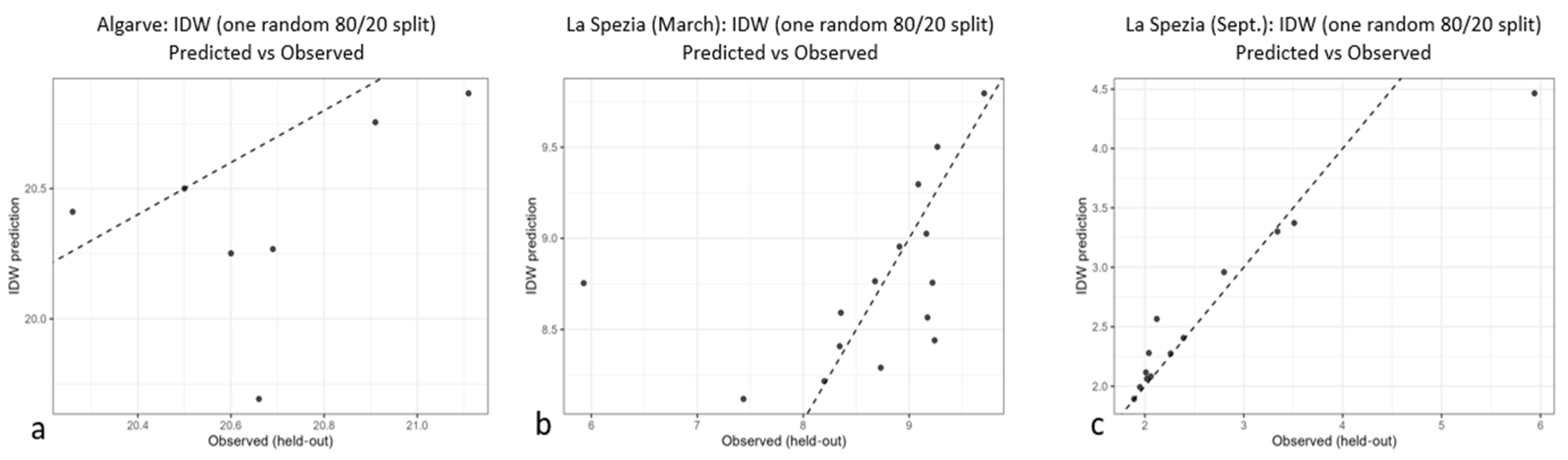
Figure A2.
MCMC diagnostics for La Spezia BK models (March and September 2024). Panels (a,b) refer to March and (c,d) to September. For each month, the top two rows show representative trace plots of key Matern/GP parameters (σ2, τ2, ϕ, ν), indicating stable post-burn-in behavior with no visible drifts. The chains explore a stationary region around their posterior modes. The bottom two rows display autocorrelation functions (ACF) for the same parameters. Autocorrelation decays within a few tens of lags, with variance terms (σ2, τ2) exhibiting faster decay than spatial parameters (ϕ, ν), which is typical in GP models. The blue dotted lines indicate the approximate 95% confidence bounds for the autocorrelation function under white-noise assumptions. These visual diagnostics are consistent with the quantitative results in Table A1 (high effective sample sizes and Geweke z-scores near zero), confirming adequate mixing and convergence for both months.
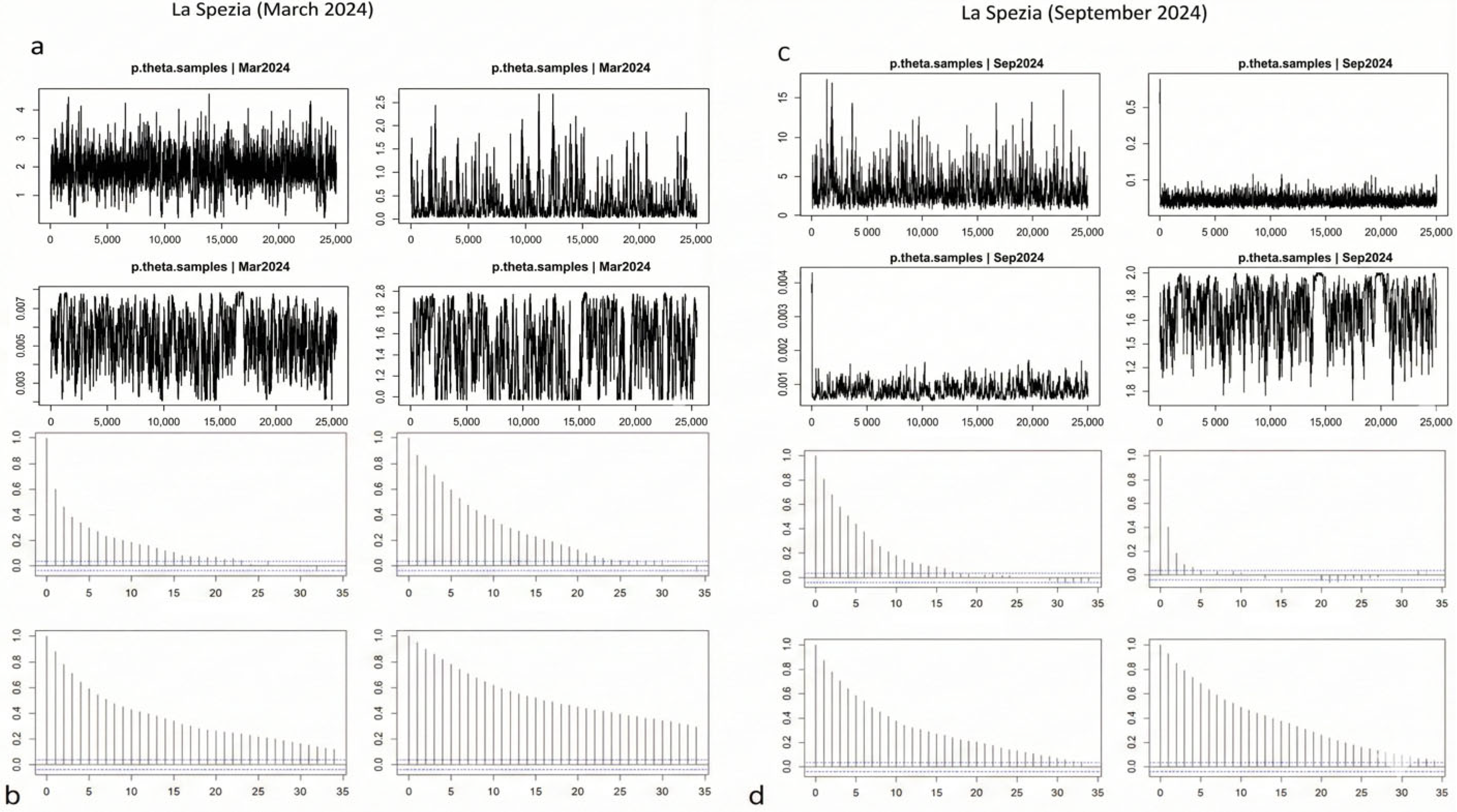
Table A4.
Repeated 80/20 CV of the IDW baseline by site/period. Entries report medians and interquartile ranges (IQR: q75–q25) across independent splits. Units: SST in °C; Chl in mg m−3. Metrics computed strictly on held-out points. Coverage95/PI-width appear only where applicable.
Table A5.
Grid-to-grid comparison between the BK 30 m chlorophyll field and Landsat OC3 (same dates). “RAW” uses the satellite values as is; “GAM-calibrated” applies the monotonic calibration of Section 4.5 to map the satellite scale to the in situ scale (evaluation only, BK fitting is unaffected). Metrics are computed over valid overlapping water pixels. Units: mg m−3.
Figure A3.
Panels (a,b): Algarve (SST, 500 m), repeated 80/20 CV with the IDW baseline (20 splits). (a) Boxplots of Bias, MAE and RMSE across splits illustrate the baseline dispersion (medians/IQR match Table A4). (b) Histogram of BK CV residuals (prediction error = BK prediction − observed) centered near zero, consistent with the empirical coverage close to or above the nominal 0.95 reported in the main text (Table 2). Panels (c,d): La Spezia Chl (30 m), independent BK vs. Landsat OC3 error distributions (for evaluation only). Histograms show Landsat—BK differences for March 2024 (c) and September 2024 (d). The dashed line marks zero error. March exhibits a pronounced positive offset prior to calibration, whereas September errors concentrate tightly around zero, in line with Table 3b and the calibrated comparisons in Table A5, Appendix A.2. Units: °C (Algarve), mg m−3 (La Spezia).
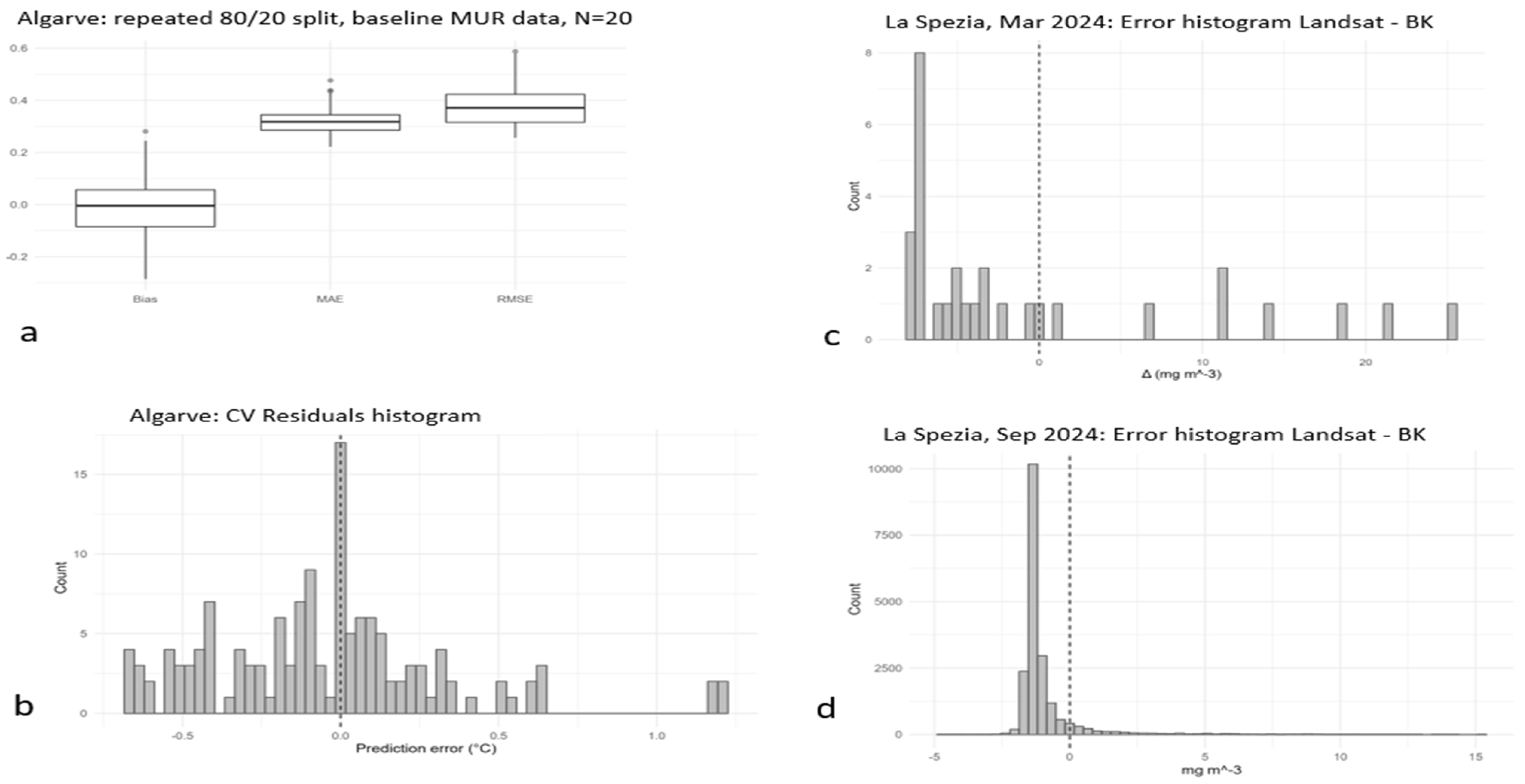
References
- Wang, R.; Pan, D.; Guo, X.; Sun, K.; Clarisse, L.; Van Damme, M.; Coheur, P.-F.; Clerbaux, C.; Puchalski, M.; Zondlo, M.A. Bridging the spatial gaps of the Ammonia Monitoring Network using satellite ammonia measurements. Atmos. Chem. Phys. 2023, 23, 13217–13234. [Google Scholar] [CrossRef] [Scilit]
- Tian, Y.; Duan, M.; Cui, X.; Zhao, Q.; Tian, S.; Lin, Y.; Wang, W. Advancing application of satellite remote sensing technologies for linking atmospheric and built environment to health. Front. Public Health 2023, 11, 1270033. [Google Scholar] [CrossRef] [Scilit]
- Zhang, J.; Li, X.; Yang, R.; Liu, Q.; Zhao, L.; Dou, B. An Extended Kriging Method to Interpolate Near-Surface Soil Moisture Data Measured by Wireless Sensor Networks. Sensors 2017, 17, 1390. [Google Scholar] [CrossRef] [Scilit] [PubMed]
- Li, J.; Heap, A.D. A review of comparative studies of spatial interpolation methods in environmental sciences: Performance and impact factors. Ecol. Inform. 2011, 6, 228–241. [Google Scholar] [CrossRef] [Scilit]
- Le, N.D.; Zidek, J.V. Interpolation with uncertain spatial covariances: A Bayesian alternative to kriging. J. Multivar. Anal. 1992, 43, 351–374. [Google Scholar] [CrossRef] [Scilit]
- Omre, H. Bayesian kriging—Merging observations and qualified guesses in kriging. Math. Geol. 1987, 19, 25–39. [Google Scholar] [CrossRef] [Scilit]
- Handcock, M.S.; Stein, M.L. A Bayesian analysis of kriging. Technometrics 1993, 35, 403–410. [Google Scholar] [CrossRef]
- Krivoruchko, K.; Gribov, A. Evaluation of empirical Bayesian kriging. Spat. Stat. 2019, 32, 100368. [Google Scholar] [CrossRef] [Scilit]
- Veronesi, F.; Schillaci, C. Comparison between geostatistical and machine learning models as predictors of topsoil organic carbon with a focus on local uncertainty estimation. Ecol. Indic. 2019, 101, 1032–1044. [Google Scholar] [CrossRef] [Scilit]
- Mishra, U.; Gautam, S.; Riley, W.J.; Hoffman, F.M. Ensemble machine learning approach improves predicted spatial variation of surface soil organic carbon stocks in data-limited northern circumpolar region. Front. Big Data 2020, 3, 528441. [Google Scholar] [CrossRef] [Scilit]
- Cui, T.; Li, X.; Zhang, L.; Du, J.; Wang, Z. A Bayesian Approach to Estimate the Spatial Distribution of Seawater Temperature Using Remote Sensing Data. Remote Sens. 2021, 13, 1234. [Google Scholar] [CrossRef] [Scilit]
- Zaresefat, M.; Derakhshani, R.; Griffioen, J. Empirical Bayesian Kriging, a Robust Method for Spatial Data Interpolation of a Large Groundwater Quality Dataset from the Western Netherlands. Water 2024, 16, 2581. [Google Scholar] [CrossRef] [Scilit]
- Takoutsing, B.; Heuvelink, G.B.M. Comparing the prediction performance, uncertainty quantification and extrapolation potential of regression kriging and random forest while accounting for soil measurement errors. Geoderma 2022, 428, 116192. [Google Scholar] [CrossRef] [Scilit]
- Bykov, K.; Höhne, M.-C.; Creosteanu, A.; Müller, K.R.; Klauschen, F.; Nakajima, S.; Kloft, M. Explaining Bayesian Neural Networks. arXiv 2021. [Google Scholar] [CrossRef] [Scilit]
- Vicedo-Cabrera, A.M.; Biggeri, A.; Grisotto, L.; Barbone, F.; Catelan, D. A Bayesian kriging model for estimating residential exposure to air pollution of children living in a high-risk area in Italy. Geospat. Health 2013, 8, 87–95. [Google Scholar] [CrossRef] [Scilit]
- Lompar, M.; Lalic, B.; Dekic, L.; Petric, M. Filling Gaps in Hourly Air Temperature Data Using Debiased ERA5 Data. Atmosphere 2019, 10, 13. [Google Scholar] [CrossRef] [Scilit]
- Senanayake, I.P.; Pathira Arachchilage, K.R.L.; Yeo, I.-Y.; Khaki, M.; Han, S.-C.; Dahlhaus, P.G. Spatial Downscaling of Satellite-Based Soil Moisture Products Using Machine Learning Techniques: A Review. Remote Sens. 2024, 16, 2067. [Google Scholar] [CrossRef] [Scilit]
- Hoff, R.M.; Christopher, S.A. Remote sensing of particulate pollution from space: Have we reached the promised land? J. Air Waste Manag. Assoc. 2009, 59, 645–675. [Google Scholar] [CrossRef] [Scilit] [PubMed]
- Agyeman, P.C.; Kebonye, N.M.; John, K.; Borůvka, L.; Vasat, R.; Fajemisin, O. Prediction of nickel concentration in peri-urban and urban soils using hybridized empirical Bayesian kriging and support vector machine regression. Sci. Rep. 2022, 12, 3004. [Google Scholar] [CrossRef] [Scilit] [PubMed]
- Shaddick, G.; Thomas, M.L.; Amini, H.; Broday, D.; Cohen, A.; Frostad, J.; Green, A.; Gumy, A.; Liu, Y.; Martin, R.V.; et al. Data Integration for the Assessment of Population Exposure to Ambient Air Pollution for Global Burden of Disease Assessment. Environ. Sci. Technol. 2018, 52, 9069–9078. [Google Scholar] [CrossRef] [Scilit]
- IOCCG. Remote Sensing of Ocean Color in Coastal, and Other Optically-Complex, Waters; Reports of the International Ocean-Color Coordinating Group, No. 3; IOCCG: Dartmouth, NS, Canada, 2000. [Google Scholar]
- Vanhellemont, Q.; Ruddick, K. Advantages of high quality SWIR bands for ocean color processing: Examples from Landsat-8. Remote Sens. Environ. 2015, 161, 89–106. [Google Scholar] [CrossRef] [Scilit]
- Relvas, P.; Barton, E.D.; Dubert, J.; Oliveira, P.; Peliz, A.; da Silva, J.; Santos, A.P. Physical oceanography of the western Iberian coastal ocean: A review and new results. Deep Sea Res. Part II Top. Stud. Oceanogr. 2007, 54, 2559–2580. [Google Scholar]
- Roberts, D.R.; Bahn, V.; Ciuti, S.; Boyce, M.S.; Elith, J.; Guillera-Arroita, G.; Hauenstein, S.; Lahoz-Monfort, J.J.; Schröder, B.; Thuiller, W.; et al. Cross-validation strategies for data with temporal, spatial, hierarchical, or phylogenetic structure. Ecography 2017, 40, 913–929. [Google Scholar] [CrossRef] [Scilit]
- Diggle, P.J.; Tawn, J.A.; Moyeed, R.A. Model-based geostatistics. J. R. Stat. Soc. Ser. C (Appl. Stat.) 1998, 47, 299–350. [Google Scholar] [CrossRef] [Scilit]
- Stein, M.L. Interpolation of Spatial Data: Some Theory for Kriging; Part of series: Springer Series in Statistics; Springer: New York, NY, USA, 1999; pp. 87–103. ISBN 0387986294. [Google Scholar] [CrossRef] [Scilit]
- Rasmussen, C.E.; Williams, C.K.I. Gaussian Processes for Machine Learning; MIT Press: Cambridge, MA, USA, 2006; pp. 84–89. [Google Scholar]
- Lindgren, F.; Rue, H.; Lindstrom, J. An explicit link between Gaussian fields and Gaussian Markov random fields: The stochastic partial differential equation approach. J. R. Stat. Soc. B 2011, 73, 423–498. [Google Scholar] [CrossRef] [Scilit]
- Poulain, P.-M.; Mauri, E.; Gerin, R.; Chiggiato, J.; Schroeder, K.; Griffa, A.; Borghini, M.; Zambianchi, E.; Falco, P.; Testor, P.; et al. On the dynamics in the southeastern Ligurian Sea in summer 2010. Cont. Shelf Res. 2020, 196, 104083. [Google Scholar] [CrossRef] [Scilit]
- Lapucci, C.; Ampolo Rella, M.; Brandini, C.; Ganzin, N.; Gozzini, B.; Maselli, F.; Massi, L.; Nuccio, C.; Ortolani, A.; Trees, C. Evaluation of empirical and semi-analytical chlorophyll algorithms in complex coastal waters of the northern Tyrrhenian and Ligurian Seas. J. Appl. Remote Sens. 2012, 6, 063565. [Google Scholar] [CrossRef] [Scilit]
- Fernandez-Tejedor, M.; Velasco, J.E.; Angelats, E. Accurate Estimation of Chlorophyll-a Concentration in the Coastal Areas of the Ebro Delta (NW Mediterranean) Using Sentinel-2 and Its Application in the Selection of Areas for Mussel Aquaculture. Remote Sens. 2022, 14, 5235. [Google Scholar] [CrossRef] [Scilit]
- Finley, A.; Banerjee, S. spBayes: Univariate and Multivariate Spatial-Temporal Modeling. R Package Version 0.4-8. 2024. Available online: https://cran.r-project.org/web/packages/spBayes/index.html (accessed on 15 July 2025).
- Gelman, A.; Carlin, J.B.; Stern, H.S.; Dunson, D.B.; Vehtari, A.; Rubin, D.B. Bayesian Data Analysis, 3rd ed.; Chapman & Hall/CRC: Boca Raton, FL, USA, 2013. [Google Scholar] [CrossRef] [Scilit]
- Finley, A.O.; Banerjee, S.; Gelfand, A.E. spBayes for Large Univariate and Multivariate Point Referenced Spatio-Temporal Data Models. J. Stat. Softw. 2015, 63, 1–28. Available online: https://www.jstatsoft.org/article/view/v063i13 (accessed on 11 September 2025). [CrossRef] [Scilit]
- Ribeiro, P.J., Jr.; Diggle, P. geoR: Analysis of Geostatistical Data. R Package Version 1.9-5. 2025. Available online: https://cran.r-project.org/web/packages/geoR/index.html (accessed on 15 September 2025).
- Shi, Y.; Zhou, X.; Yang, X.; Shi, L.; Ma, S. Merging Satellite Ocean Color Data with Bayesian Maximum Entropy Method. IEEE J. Sel. Top. Appl. Earth Obs. Remote Sens. 2015, 8, 3294–3304. [Google Scholar] [CrossRef] [Scilit]
- He, S.; Wong, S.W.K. Spatio-temporal data fusion for the analysis of in-situ and remote sensing data using the INLA-SPDE approach. Spat. Stat. 2024, 64, 100863. [Google Scholar] [CrossRef] [Scilit]
- Obenour, D.R.; Gronewold, A.D.; Stow, C.A.; Scavia, D. Using a Bayesian hierarchical model to improve Lake Erie cyanobacteria bloom forecasts. Water Resour. Res. 2014, 50, 7848–7860. [Google Scholar] [CrossRef] [Scilit]
- Wang, Y.; Hu, X.; Chang, H.H.; Waller, L.A.; Belle, J.H.; Liu, Y. A Bayesian downscaler model to estimate daily PM2.5 levels in the conterminous US. Int. J. Environ. Res. Public Health 2018, 15, 1999. [Google Scholar] [CrossRef] [Scilit]
- Truong, P.N.; Heuvelink, G.B.M.; Pebesma, E. Bayesian area-to-point kriging using expert knowledge as informative priors. Int. J. Appl. Earth Obs. Geoinf. 2014, 30, 128–138. [Google Scholar] [CrossRef] [Scilit]
- Cui, H.; Stein, A.; Myers, D.E. Extension of spatial information, Bayesian kriging and updating of prior variogram parameters. Environmetrics 1995, 6, 373–384. [Google Scholar] [CrossRef] [Scilit]
- Beckers, J.-M.; Rixen, M. EOF calculations and data filling from incomplete oceanographic data series. J. Atmos. Ocean. Technol. 2003, 20, 1839–1856. [Google Scholar] [CrossRef] [Scilit]
- Barth, A.; Alvera-Azcárate, A.; Beckers, J.-M. DINCAE 1.0: A convolutional autoencoder with error estimates to reconstruct sea surface temperature satellite observations. Geosci. Model Dev. 2020, 13, 1609–1622. [Google Scholar] [CrossRef] [Scilit]
- Gao, F.; Masek, J.G.; Schwaller, M.; Hall, F.G. On the blending of the Landsat and MODIS surface reflectance: Predicting daily Landsat surface reflectance. IEEE Trans. Geosci. Remote Sens. 2006, 44, 2207–2218. [Google Scholar] [CrossRef] [Scilit]
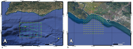
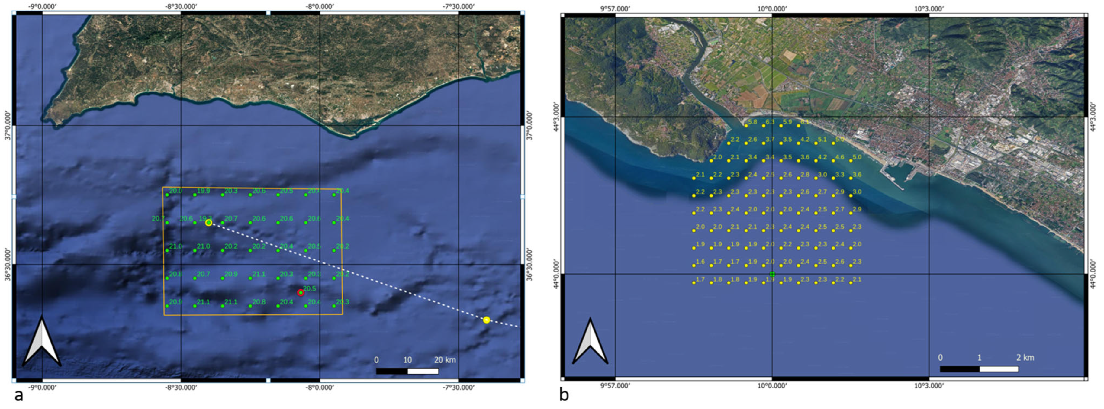
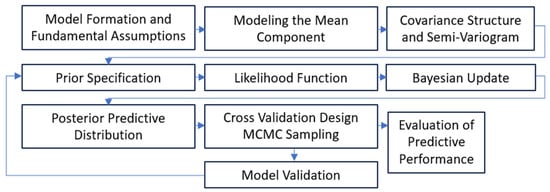
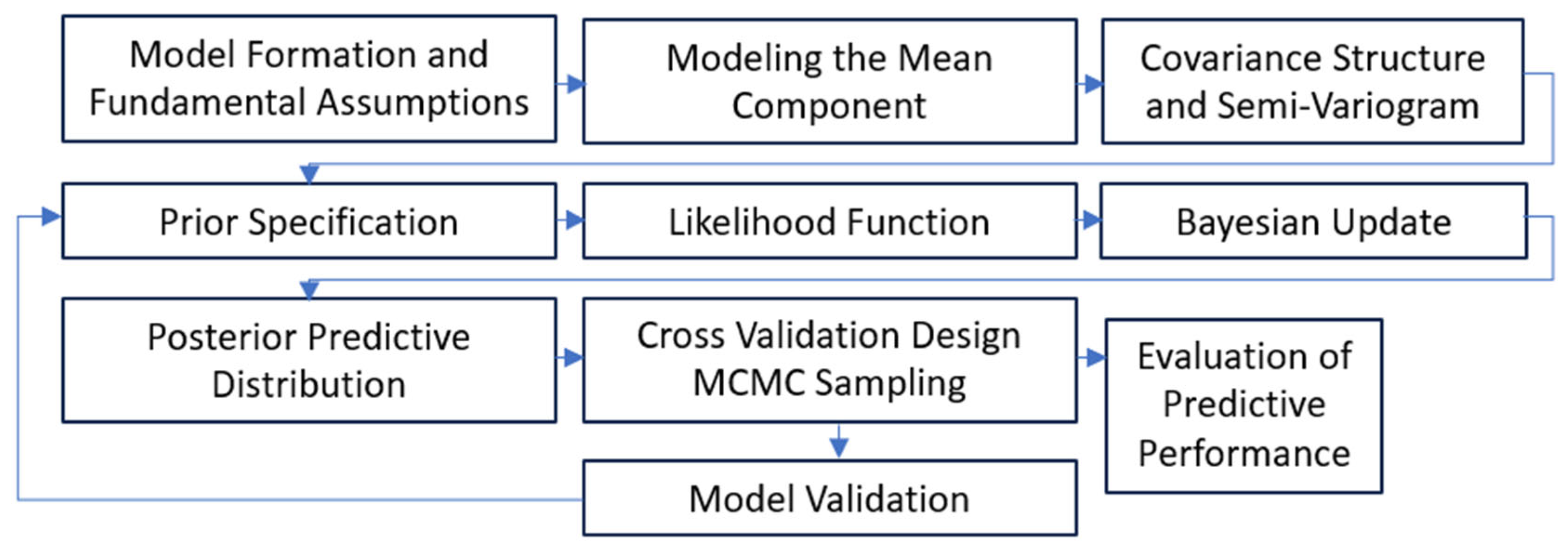
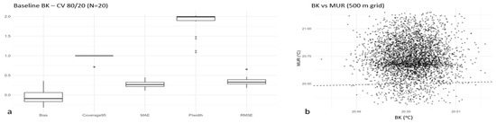
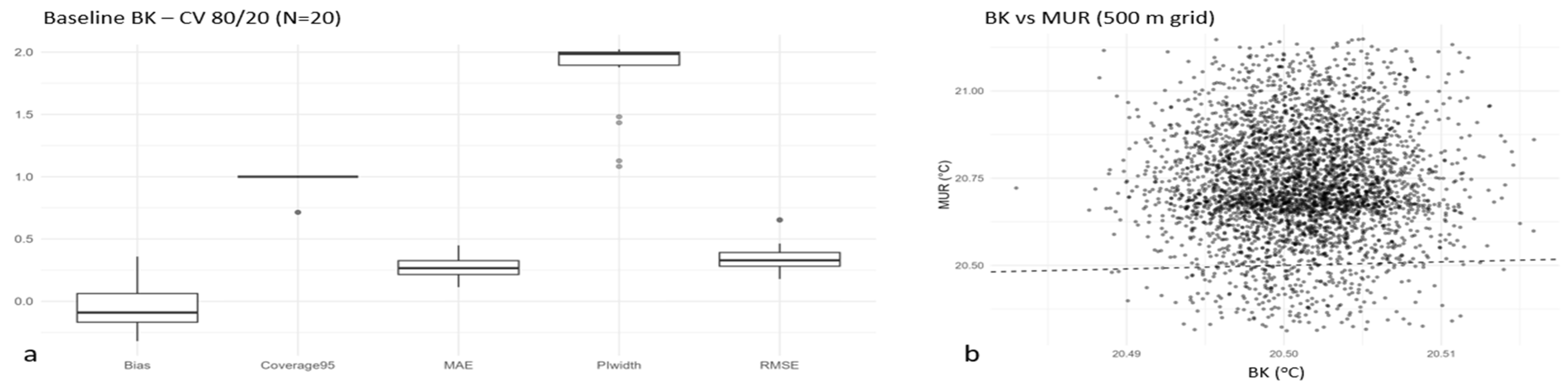
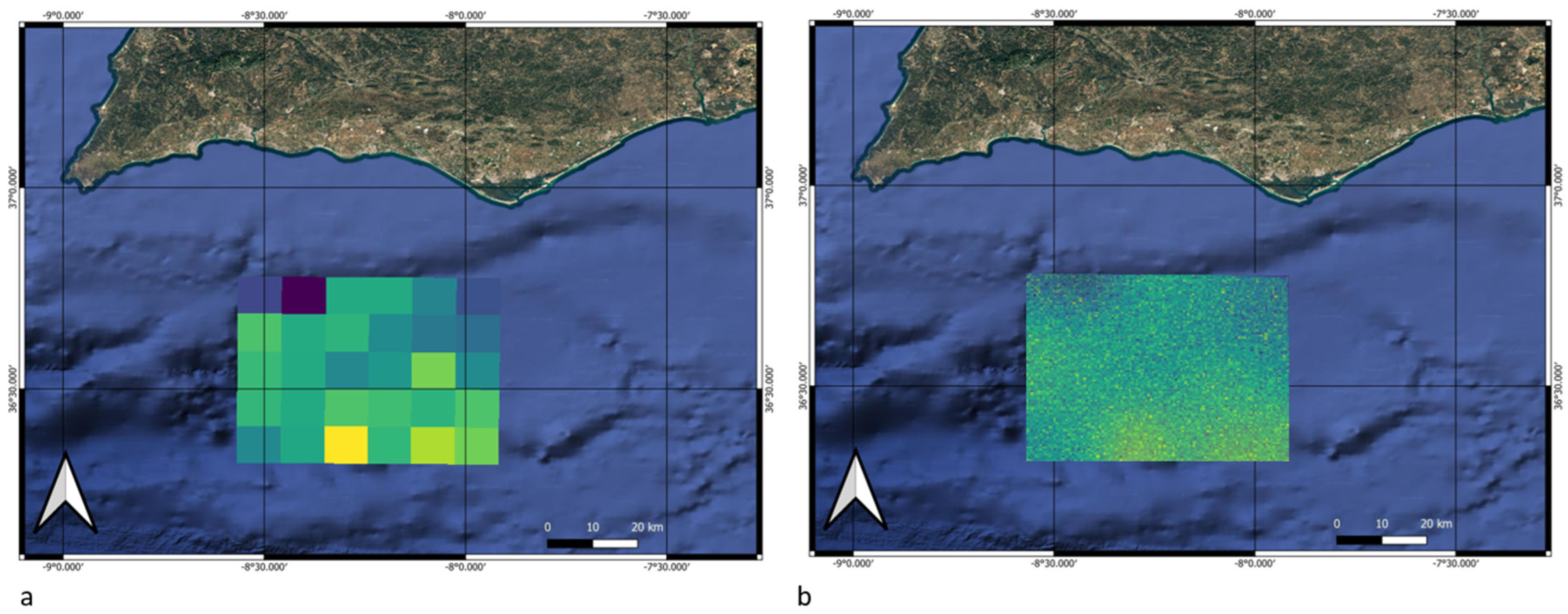
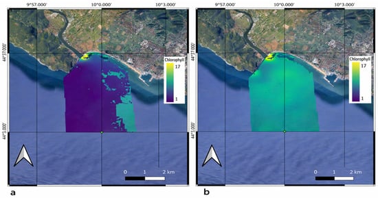
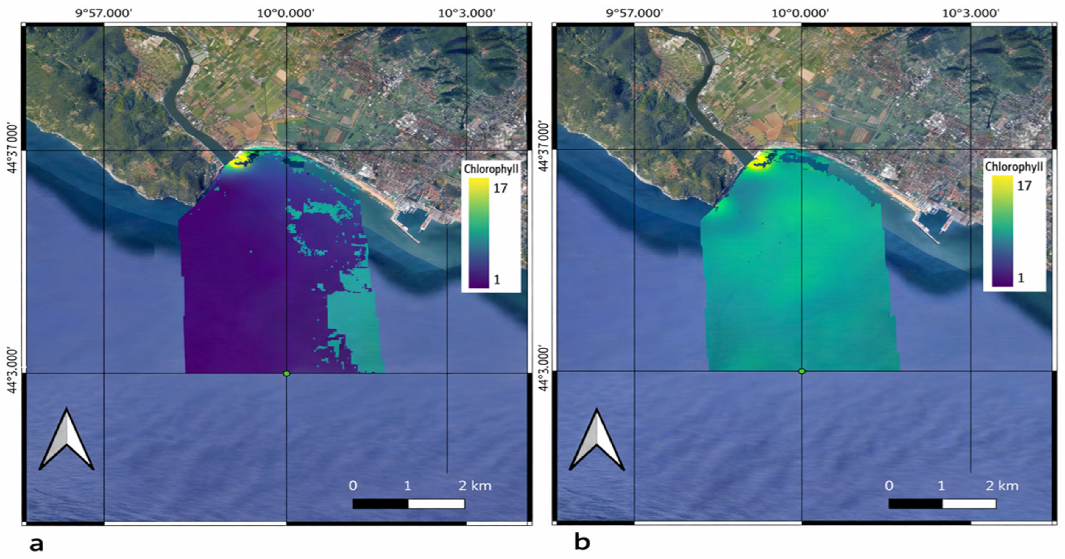
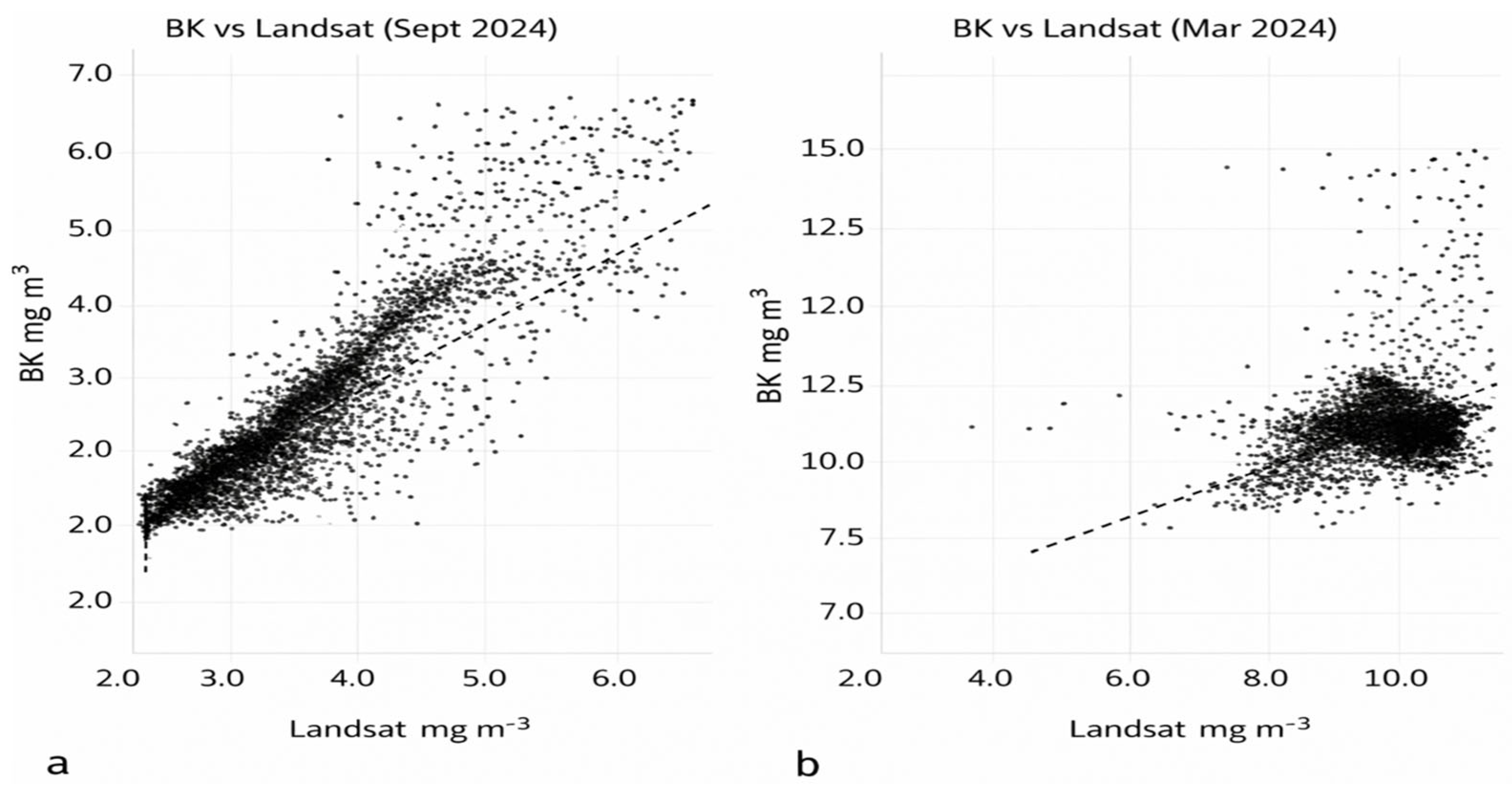

Disclaimer/Publisher’s Note: The statements, opinions and data contained in all publications are solely those of the individual author(s) and contributor(s) and not of MDPI and/or the editor(s). MDPI and/or the editor(s) disclaim responsibility for any injury to people or property resulting from any ideas, methods, instructions or products referred to in the content. |
© 2026 by the authors. Licensee MDPI, Basel, Switzerland. This article is an open access article distributed under the terms and conditions of the Creative Commons Attribution (CC BY) license.