


Highlights
- NEE temporal dynamics of restored and natural mangrove forests were analyzed.
- Evaluated how different variable schemes and modeling approaches affected the performance of NEE simulation.
- High-resolution (30 m) regional mangrove NEE dynamics were simulated.
- A data-driven basis for improving blue carbon assessment, monitoring restoration effectiveness, and supporting climate mitigation strategies in coastal ecosystems was constructed.
Abstract
Mangrove ecosystems are important blue carbon systems and play a critical role in understanding carbon cycling and responses to climate change. However, accurate regional estimation of Net Ecosystem Exchange (NEE) remains challenging due to the environmental complexity and spatial heterogeneity. This study combined eddy covariance observations from four mangrove sites along China’s southeastern coast (natural and restored mangrove forests) with multi-source remote sensing and environmental reanalysis data to construct three variable schemes (site observations only, with added vegetation indices, and comprehensive multi-source variables). We compared three machine learning models for daily NEE prediction, including eXtreme Gradient Boosting (XGBoost), Random Forest (RF), and Support Vector Machine (SVM). The results showed that: (1) Restored and natural mangroves exhibited similar temporal NEE dynamics and consistently functioned as carbon sinks, restored mangrove sites showed greater cross-site variability. Among the study sites, CN-LZR exhibited the strongest cumulative carbon uptake. (2) Scheme 3 combined with the XGBoost algorithm achieved the highest predictive accuracy, reaching an R2 of 0.73 across sites. Differences among machine learning models were primarily associated with their ability to capture nonlinear interactions between atmospheric and hydrological variables, with tree-based models outperforming SVM. (3) SHAP analysis indicated that radiation-related variables were the dominant drivers of NEE, while hydrological influences were site-dependent; and (4) Regional upscaling indicated that all sites consistently functioned as long-term carbon sinks, with CN-LZR exhibiting slightly higher daily mean carbon uptake than the other sites. This study presented the first machine learning framework for estimating daily-scale NEE in mangroves, providing methodological and data support for regional carbon flux assessment and blue carbon management.
1. Introduction
Blue carbon is recognized as one of the essential ways to mitigate climate change, achieved through the conservation, restoration, and sustainable management of ecosystems to enhance carbon sequestration and resilience [1,2]. The mangrove ecosystem is among the most important coastal blue ecosystems. This ecosystem has a high capacity to store and sequester carbon, even higher than that of terrestrial forest ecosystems [3,4]. However, the alternating land–water conditions in mangrove environments introduce uncertainties to carbon monitoring. Therefore, quantifying and understanding carbon fluxes in mangrove ecosystems is critical for informing effective climate mitigation policies [5].
Net ecosystem exchange (NEE) quantifies the exchange of carbon dioxide between an ecosystem and the atmosphere, representing the balance between ecosystem respiration (RE) and gross primary production (GPP). GPP is the total carbon fixed by photosynthesis, whereas RE encompasses the total carbon released through both plant and soil microbial respiration. A negative NEE value indicates a net uptake of CO2 from the atmosphere, as NEE is defined as the difference between RE and GPP. NEE is commonly measured at field sites using the eddy covariance (EC) system, which currently provides the most accurate ecosystem-scale flux observations by calculating the covariance between high-frequency vertical wind speed and fluctuations in carbon dioxide concentration [6,7]. Despite its accuracy, EC tower observations face several limitations. The land surface area contributing to a single EC tower’s measurement typically extends only a few hundred meters from the site, with its precise extent modulated by factors such as tower height, wind direction, and canopy structure [8]. In a subtropical mangrove ecosystem, approximately 80% of the flux contribution originated from an area within 200 m of the tower [9]. To satisfy the fundamental assumptions of the observational technique, installation sites must exhibit relatively uniform and open environmental conditions. To meet the fundamental assumptions of the EC technique, installation sites must exhibit relatively uniform and open environmental conditions. The high costs and stringent site requirements of EC towers limit their deployment, hindering the accurate estimation of regional-scale ecosystem carbon budgets.
Accurate monitoring of NEE dynamics in coastal wetlands across spatial scales remains challenging due to multiple factors. The carbon cycle in mangrove ecosystems extends beyond soil–atmosphere exchanges and is strongly influenced by oceanic processes. Environmental drivers such as tidal inundation introduce complex effects on carbon cycling. Short-term measurements have shown that CO2 (and CH4) fluxes from soil and stems vary substantially with tidal cycles [10]. Tidal inundation can indirectly affect biogenic carbon fluxes by influencing oxygen availability in surface sediments [11,12]. Many existing terrestrial ecosystem data-driven approaches or data products have limited applicability in mangrove ecosystems. Additionally, differences in structure and management between artificial and natural mangroves may result in variations in carbon storage, photosynthetic activity, and soil carbon accumulation [13,14,15]. As artificial mangroves play a critical role in coastal restoration and blue carbon initiatives, their NEE characteristics require evaluation relative to those of natural mangroves. Publicly available eddy covariance (EC) observations in mangrove ecosystems are extremely limited, primarily due to the technical and operational challenges posed by tidal inundation and dynamic hydrological conditions. For instance, the widely adopted FLUXNET2015 dataset contains almost no mangrove EC sites. However, the increasing accessibility of mangrove flux observations has facilitated the rapid development of mangrove flux simulation studies. NEE integrates both photosynthetic carbon uptake and ecosystem respiration, which introduces greater uncertainty into its estimation. Most current research has focused on GPP, which is driven by photosynthetic processes. For example, a Gaussian Process Regression model [16] applied to estimate GPP achieved high accuracy (R2 = 0.90, RMSE = 0.92 gC m−2 day−1). A substantial research gap remains in the investigation of NEE in mangrove regions, particularly using high-resolution remote sensing data at the daily time scale.
There are several approaches to accurately estimating NEE at the regional scale, including process-based modeling and data-driven machine learning. Process-based ecological models simulate the transfer of carbon between the atmosphere and soils by explicitly representing biophysical and biogeochemical processes. While these models offer strong interpretability and process attribution, their regional application is often limited by complex parameterization, high data requirements, and insufficient representation of hydrological and tidal processes in mangrove ecosystems [17]. The mangrove-specific MCAT-DNDC model [18] is driven by approximately 40 input parameters, including numerous vegetation physiological and soil biogeochemical variables that are difficult to obtain at the regional scale. Alternatively, EC-tower-driven statistical or machine learning (ML) models extrapolate site-level flux measurements by establishing relationships with remote sensing and meteorological data. This approach has achieved R2 values of 0.7–0.9 for NEE in boreal forests [19]. Despite the increasing application of machine learning in ecosystem carbon research, there is a lack of systematic evaluation of appropriate input variables for ML-based NEE estimation in mangrove ecosystems.
Daily-scale NEE serves as a crucial link between instantaneous biophysical processes and long-term carbon budgets, establishing a temporal foundation for integrating machine learning models with satellite data. Although machine learning methods effectively capture nonlinear interactions among multiple NEE drivers, the relationships between environmental drivers and NEE are dependent on the timescale. These relationships shift with temporal aggregation as the relative contributions of photosynthesis, respiration, and vegetation regulation vary, yet such variations in these drivers have rarely been examined in mangrove ecosystems [20]. In particular, the variation characteristics of NEE and potential differences in its driving factors across temporal scales between artificial and natural mangrove wetlands remain poorly understood. ML algorithms may exhibit different performance when applied to predict the fluxes in vegetation ecosystems. A meta-analysis of 178 model records across 40 studies and multiple ecosystem types indicated that model accuracy is strongly dependent on predictor selection, temporal and spatial scales, and data quality [21]. The Extreme Gradient Boosting (XGBoost) model achieved higher estimation accuracy than other ML methods for mangrove GPP [22]. Support vector machines (SVM) and random forest (RF) achieved the highest average predictive accuracy [23] in water flux prediction. Variability in model performance across studies has been reported, underscoring the need for systematic model evaluation. Moreover, most existing mangrove NEE studies rely primarily on site-level meteorological and flux measurements [20]. Limited integration of satellite-derived vegetation and environmental indicators restricts their spatial applicability. Therefore, comparing different models and variable schemes is necessary to improve understanding of time-scale-dependent drivers of mangrove NEE in both artificial and natural ecosystems and to support NEE estimation by integrating satellite-derived spatial information.
There remains a significant research gap in integrating satellite remote sensing data into machine learning-based mangrove NEE estimation for regional-scale applications that consider mangrove ecosystem characteristics. This study aimed to address this research gap by focusing on artificial and natural mangrove wetlands along the southeastern coast of China and applying machine learning approaches to estimate and simulate site-scale NEE over a 25-year period. Specifically, the study (1) compared temporal characteristic environmental controls and NEE dynamics between two natural and two restored mangrove sites to evaluate cross-site variability; (2) integrated remote sensing indicators with coastal environmental variables to construct three modeling schemes and identify the optimal machine learning framework for NEE prediction; and (3) applied the optimal model for long-term regional upscaling and provide a reference for regional NEE estimation in mangrove ecosystems.
2. Materials and Methods
2.1. Study Areas
This study was conducted across four mangrove sites in three coastal provinces of southeastern China (Figure 1), comprising two restored and two natural mangrove sites. Although all sites are estuarine, the mangrove ecosystems exhibit significant biological variation in vegetation composition and canopy structure. Detailed site characteristics are summarized in Table S1. From north to south, the study sites include:
Figure 1.
Study area and EC tower locations. The suffix “N” indicates natural mangrove sites, and “R” indicates restored mangrove sites. From north to south, the sites are: Restored mangroves in Aojiang County, Wenzhou City, Zhejiang Province (CN-AJR); Natural mangroves in Yunxiao County, Zhangzhou City, Fujian Province (CN-YXN); Natural mangroves in Gaoqiao Town, Lianjiang City, Guangdong Province (CN-GQN); and Restored mangroves in Leizhou City, Guangdong Province (CN-LZR).
- (i)
- Aojiang Restored Mangroves site (CN-AJR) is located in Aojiang County, Zhejiang Province (27°34′58″N, 120°34′13″E), encompassing approximately 11 hectares. This site represents the northern distribution limit of mangroves in China.
- (ii)
- Natural Mangrove site (CN-YXN) in Yunxiao County, Zhangzhou City, Fujian Province is situated in the Zhangjiang Estuary Mangrove National Nature Reserve (23°55′26.4″N, 117°24′52.9″E).
- (iii)
- Natural Mangrove site (CN-GQN) in Gaoqiao Town, Lianjiang City, Guangdong Province, is located within Yingluo Bay at the northern edge of the Beibu Gulf (21°34′3.05″N, 109°45′22.32″E). The mangrove forest is characterized by its natural, contiguous, and large-scale spatial distribution and is managed by Guangdong Zhanjiang Mangrove National Nature Reserve. The mangrove stand at Gaoqiao Station has an estimated age exceeding 100 years.
- (iv)
- Restored Mangrove site (CN-LZR) is located in Fucheng Town, Leizhou City, Guangdong Province (20°56′24″N, 110°09′44″E), where the mangroves extend along the coast in a north–south direction. Planted in the 1990s, the stand surpassed 20 years of age during the study period.
2.2. Datasets
2.2.1. Site Observation Data
Half-hourly NEE data and associated meteorological variables, such as air temperature (TA) and photosynthetic photon flux density (PPFD), were compiled from publicly available datasets across multiple EC sites [24,25]. Observational data from these EC sites were processed using a standardized procedure. First, high-frequency (10 Hz) raw measurements from open-path infrared gas analyzers were processed into half-hourly using EddyPro software, following standard FLUXNET protocols [6,26]. Subsequent post-processing steps, including low-turbulent filtering and gap-filling, were conducted using the REddyProc package in R or its online tool [27]. This consistent post-processing methodology ensures the comparability of publicly available EC datasets from different site studies. Table S1 provides detailed information on the CO2 measurement instruments and versions of data processing software (EddyPro) employed at each site.
The datasets cover the periods 2020–2022 for the CN-AJR site, 2009–2012 for the CN-YXN site, 2015–2017 for the CN-LZR site, and 2009–2015 for the CN-GQN site [24,25]. For half-hourly observations, time stamps were first examined to ensure that each day contained 48 half-hourly records. Missing records or values were identified and set to NA. Observations that did not conform to variable definitions were corrected or excluded. Negative nighttime values of photosynthetic photon flux density (PPFD) were set to zero. Outliers for each variable were identified using a three-standard-deviation criterion (mean ± 3 × SD). To reduce potential biases from data interpolation, only days with more than 46 valid half-hourly records were included in daily-scale aggregation. Water level (WL) data were obtained from pressure gauges near the flux tower or from tide level stations upstream of the estuary. Except for the CN-AJR site, WL observations at other sites were available for only one to two years, and their temporal coverage did not fully overlap with NEE measurements. To ensure consistency and data quality at the daily scale, daily mean values were calculated only for days that met the minimum record requirement. As a result, the number of available daily-scale records of NEE, TA, PPFD, and WL at each site was as follows: 1009 for CN-AJR, 674 for CN-GQN, 215 for CN-LZR, and 321 for CN-YXN. This dataset served as the foundation for the subsequent variable scheme, which was implemented using only site-level observational data.
2.2.2. Remote Sensing–Based Index
Vegetation status and environmental dynamics at the study sites were characterized using remote sensing-based indices. Image collections from Landsat 5, 7, 8, and 9 were integrated into a unified Landsat dataset covering the period from 2000 to 2025. This dataset used the Landsat Collection 2 Tier 1 Level-2 Science product, which has been radiometrically calibrated and atmospherically corrected to ensure accurate, temporally consistent surface reflectance across all sensors.
To improve data quality, cloud shadows, clouds, and snow-contaminated pixels were identified and removed using the quality assurance bands included with the Landsat products. Using the calibrated spectral bands, a suite of vegetation and water indices was calculated. Three widely used vegetation indices were selected to represent vegetation conditions: the Normalized Difference Vegetation Index (NDVI), the Enhanced Vegetation Index (EVI), and the Mangrove Vegetation Index (MVI). Additionally, three water-related indices were employed to characterize hydrological and surface water dynamics: the Normalized Difference Water Index (NDWI), the Modified NDWI (mNDWI), and the Land Surface Water Index (LSWI). These indices provide complementary information on vegetation vigor, canopy structure, and surface water conditions and have been extensively applied for monitoring and assessing vegetation ecosystem changes over extended temporal scales [28].
For Landsat 5 and Landsat 7, the blue, green, red, near-infrared (NIR), and shortwave infrared (SWIR) bands correspond to Bands 1, 2, 3, 4, and 5, respectively. For Landsat 8 and Landsat 9, the corresponding bands are Bands 2, 3, 4, 5, and 6. These bands were consistently used to calculate vegetation indices (NDVI, EVI, and MVI) and water-related indices (NDWI, mNDWI, and LSWI) across different Landsat sensors.
To generate a daily 30 m vegetation and water index time series with high temporal resolution, MODIS MCD43A4 data, which provide daily observations, were integrated with and bias-corrected using 30 m Landsat observations. A Savitzky–Golay (S–G) filter with a third-order polynomial and a window size of 13 was applied to the MODIS index time series to suppress residual noise and mitigate short-term temporal variability. The bias correction was linearly interpolated to a daily resolution over the entire study period and then added to the S–G smoothed MODIS indices, reconstructing a daily 30 m vegetation and water index time series. The bias correction was performed using Landsat observations as the reference, with 80% of the available Landsat data used for bias calibration and the remaining 20% reserved for independent validation. The reconstructed NDVI achieved an R2 of 0.66 and a root mean square error (RMSE) of 0.16 during validation (Figure S1).
2.2.3. Regional Meteorological and Environmental Data
Meteorological and environmental datasets used in predictive modeling and regional upscaling (Table S2) of NEE were mainly derived from the ERA5-Land reanalysis dataset, the Hybrid Coordinate Ocean Model (HYCOM), and the Moderate Resolution Imaging Spectroradiometer (MODIS) Terra and Aqua combined Photosynthetically Active Radiation Level-3 gridded product (MCD18C2.062).
ERA5-Land provides temporally consistent climate variables at an hourly temporal resolution and a spatial resolution of 0.1° × 0.1° [29]. From this dataset, we extracted several meteorological and land surface variables, including surface solar radiation downwards (Rg), 2 m air temperature (Tair), soil temperature at level 1 (Tsoil), surface pressure (PA), surface latent heat flux (LE), total precipitation, and leaf area index of high vegetation (LAI). VPD and relative humidity (RH) were calculated from Tair and 2 m dew point temperature. In addition, photosynthetically active radiation (PAR) was obtained from the MODIS MCD18C2 product, which provides global estimates at a 3-hourly temporal resolution and a spatial resolution of 0.05° × 0.05° [30]. To account for marine and tidal influences on mangrove ecosystems, sea surface temperature (Twater) and sea surface salinity (SSS) were obtained from HYCOM, a data-assimilative ocean model that employs a hybrid isopycnal-sigma-pressure coordinate system. The HYCOM data were obtained as a gridded product on 0.08° × 0.08°,which was generated by using a bilinear interpolation from a native Mercator-curvilinear grid [31]. A bias-based simple statistical downscaling approach was applied to ensure spatial consistency with Landsat data at 30 m resolution under conditions of limited data availability [32,33]. All gridded datasets were first resampled to 30 m using a nearest-neighbor approach. The resampled values were then bias-corrected using site-level available observations.
2.3. Site-Level Comparison and Temporal Correlation Analysis
To systematically evaluate the characteristics of ecosystem carbon fluxes across multiple sites, continuous half-hourly flux and meteorological observations from four sites (CN-GQN, CN-LZR, CN-YXN, and CN-AJR) were integrated and analyzed using two complementary aggregation strategies.
First, NEE were aggregated for temporal pattern characterization by using time as a categorical variable, including (i) mean diurnal cycles averaged across half-hourly clock-time categories from 0.0 to 23.5 h, (ii) mean seasonal patterns based on day-of-year (DOY), and (iii) annual cumulative fluxes. These analyses were used to compare temporal structures and cumulative carbon exchange among sites.
Second, the half-hourly observations were continuously aggregated into hourly, daily, and monthly time series based on predefined time labels. At each temporal scale, correlation analyses were conducted to quantify how relationships between NEE and environmental drivers changed with increasing temporal aggregation.
Four meteorological variables were included: PPFD, TA, VPD, and WL. Six vegetation indices were considered: EVI, NDVI, MVI, LSWI, NDWI, and mNDWI. NEE served as the primary response variable. In addition, exploratory analyses were performed to assess correlation patterns across a wider range of temporal scales (1–200 days).
2.4. NEE Prediction Scheme
To explore the contributions of site-based observations, remote sensing indicators, and reanalysis data to NEE prediction in mangrove ecosystems, three variable schemes were developed. Three distinct variable schemes were constructed to assess the predictive contributions of site-based observational variables (Scheme 1), site-based and satellite-derived indicators (Scheme 2), and satellite-derived and reanalysis-based variable scheme (Scheme 3) in NEE estimation. Three commonly used ML models, including XGBoost, Random Forest (RF), and Support Vector Machine (SVM), were applied. Model performance was evaluated at individual sites as well as across all sites to examine the potential for cross-site generalization. Finally, NEE will be expanded across all sites, with the annual spatial extent of mangrove forests delineated by the corresponding year’s 30m-resolution mangrove mapping results (2000, 2010, 2015, 2020) [34]. For years without available mangrove mapping data (e.g., 2005 and 2025), we employed manual interpretation to update the regional mangrove distribution, using the most recent mangrove map and the composite average imagery from the corresponding year. Manual interpretation is a common approach for validating, modifying, and updating datasets based on existing reference data [35].
2.4.1. Variable Frameworks for NEE Prediction
Scheme 1 included site-synchronized meteorological and environmental variables for NEE estimation. Scheme 2 was developed by extending Scheme 1 to include 30 m daily vegetation and moisture indices derived from remote sensing data. A comparative analysis between Scheme 1 and Scheme 2 provides a systematic assessment of the contribution of remote sensing indicators to improve NEE estimation and enhance understanding of their utility in capturing the spatiotemporal dynamics of mangrove carbon exchange.
Scheme 3 was developed based on the characteristic carbon cycling processes of mangrove ecosystems and data availability, and integrates reanalysis-based meteorological variables with satellite-derived observations for modeling and evaluation. Based on the ecological features of the mangrove carbon cycle and data availability, variables influencing mangrove carbon fluxes were grouped into four components [36,37,38]: atmosphere, land, sea, and mangrove (Figure S2). Variables in the atmosphere and land categories are broadly comparable to those commonly used in terrestrial ecosystem studies and primarily represent controls related to radiation, temperature, and water availability. Vegetation indices were selected as key mangrove variables because they provide measurable proxies for photosynthetic activity, canopy structure, and plant water status [39]. Mangrove carbon exchange is not only controlled by terrestrial conditions but also strongly influenced by marine processes, particularly tides. Periodic tidal inundation changes salinity and water temperature, which in turn exert indirect yet persistent effects on carbon fluxes. To capture these effects, this study includes sea-related variables such as salinity, sea surface temperature, and remotely sensed moisture indices, depending on the availability of data [40]. The specific variables and valid data numbers included in each feature scheme and their corresponding predictive performance across sites are summarized in Table 1 and Tables S3–S5.
Table 1.
Description of feature schemes and associated variables.
2.4.2. Machine Learning (ML) Prediction Methods
To address the reported variability in performance among different ML approaches, three widely used ML methods and variable schemes were systematically compared [41]: XGBoost, RF, and Support Vector Machine (SVM). Five-fold cross-validation was employed to evaluate the performance of these methods.
XGBoost is an ensemble learning algorithm based on the gradient boosting framework [42,43]. In XGBoost, the model is trained by sequentially adding decision trees, where each newly constructed tree learns from the error information generated by the predictions of the previous iterations. This process progressively corrects the model’s predictions. For regression tasks, the final prediction is generated by an additive model that sums the outputs of all individual trees. XGBoost incorporates parallel computation, regularization, and sparsity-aware algorithms to balance prediction accuracy, computational efficiency, and model generalization. In this study, key parameters in the XGBoost model were optimized, including the learning rate (eta), maximum tree depth (max_depth), minimum child weight (min_child_weight), subsampling ratio (subsample), column subsampling ratio (colsample_bytree), minimum loss reduction (gamma), and L1 and L2 regularization terms (alpha and lambda).
RF is an ensemble learning algorithm based on the Bagging technique [44]. In RF, multiple independent decision trees are constructed, each trained on a bootstrap sample randomly drawn with replacement from the original training set. A random subset of input features is used for node splitting during each tree’s construction, introducing double randomness to the model training. For regression tasks, the final prediction is obtained by averaging the predictive values of all constituent trees. By training decision trees in parallel, reducing model variance, and incorporating feature randomness, RF effectively balances predictive capability, computational efficiency, and generalization performance [45]. In this study, key hyperparameters in the RF model were optimized, including the number of trees in the ensemble (ntree), the number of candidate predictors randomly selected at each split (mtry), and the minimum terminal node size (nodesize).
SVM is a classic supervised learning algorithm based on statistical learning theory and structural risk minimization. SVM seeks to identify an optimal separating hyperplane in the feature space that maximizes the margin between different classes. Kernel-based methods are employed to address complex nonlinear problems, and the selection of different kernel functions enables adaptation to diverse data patterns. SVMs are particularly suitable for large datasets and have been widely applied in various fields of data analysis. Key hyperparameters in the SVM model were optimized, including the penalty parameter controlling the trade-off between model complexity and training error (cost), the kernel width parameter governing the flexibility of the radial basis function (gamma), and the epsilon-insensitive loss parameter defining the tolerance margin for regression errors (epsilon).
All methods were implemented in the R environment (version 4.5.1). To ensure comparability of model performance across different machine learning approaches, a unified hyperparameter tuning procedure was adopted for all models. Initially, a set of hyperparameters reported as robust in previous studies was used as a baseline, around which a small-range grid search space was constructed for key parameters controlling model complexity. Candidate parameter sets were generated by uniform sampling within narrow intervals. When the parameter space was high-dimensional, a random subset of parameter combinations was selected to balance tuning precision and computational cost. Five-fold cross-validation was then employed to evaluate the performance of each candidate parameter set, with the mean validation root mean squared error (RMSE) used as a unified model selection criterion. Model-specific adaptations were applied: for XGBoost, an early stopping mechanism was introduced during training to determine the optimal number of boosting iterations; for Random Forest and Support Vector Machine, hyperparameters were directly optimized based on cross-validation results. The detailed hyperparameter configurations of each model are listed in Table S3.
2.4.3. Model Performance Evaluation
Model performance was evaluated using multiple metrics calculated on the validation set, including the coefficient of determination (R2), RMSE, and mean absolute error (MAE). R2 quantified the proportion of variability in observed net ecosystem exchange (NEE) explained by the model, whereas RMSE and MAE measured absolute prediction errors with differing sensitivity to outliers.
where and represent the i-th observed and predicted values, denotes the mean of all observed values, and n is the total number of observations.
2.5. SHAP-Based Interpretation of Daily NEE Predictions
To understand the contribution of predictor variables to daily NEE estimates, we employed the Shapley Additive Explanation (SHAP) framework in combination with the XGBoost model. SHAP quantifies feature importance by decomposing model predictions into additive contributions from individual predictors, where each SHAP value represents the average marginal contribution of a given variable across all possible combinations of the remaining features. This formulation provides a theoretically consistent means of attributing both the magnitude and direction of each predictor’s influence on daily NEE estimates, while effectively capturing nonlinear relationships and complex feature interactions inherent in tree-based models.
The SHAP–XGBoost framework has been successfully applied in previous studies analyzing carbon fluxes. In this study, SHAP analysis was implemented using the SHAP for xgboost package in R, which follows the TreeSHAP principle to enable efficient and exact computation of Shapley values by leveraging the internal structure of tree-based ensemble models such as XGBoost. SHAP explains the predictive behavior of a trained model rather than the underlying ecosystem processes directly; its reliable application for feature contribution assessment requires a well-fitted model with satisfactory predictive performance. Variable interpretation was therefore conducted on the final selected XGBoost-based modeling scheme.
3. Results
3.1. Comparision of NEE at Different and Driver Analysis
NEE demonstrated distinct temporal dynamics and variability at hourly, daily, and yearly scales (Figure 2). At the diurnal scale, the mean diurnal NEE curves of the restored sites (CN-AJR and CN-LZR) were similar to those of the natural sites (CN-GQN and CN-YXN). Both restored and natural forests exhibited consistent diurnal NEE patterns, characterized by alternating positive and negative fluctuations during the photoperiod and a peak in carbon uptake near noon. However, the restored sites showed markedly larger inter-site variability and wider standard deviation ranges, whereas the natural sites exhibited greater consistency. At the daily scale, mean NEE values of both restored and natural sites were negative, indicating that both sites acted as a net carbon sink at the daily timescale. NEE values generally fluctuated between 0 and −5 μmol CO2 m−2 s−1, with no pronounced seasonal variation observed in either restored or natural sites. Consistent with the diurnal pattern, restored sites exhibited greater site variability in daily NEE compared with natural sites. At the annual scale, the cumulative annual NEE values of all sites were consistently negative, ranging from approximately −585 to −1213 g C m−2 yr−1, indicating that both restored and natural mangrove ecosystems functioned as strong carbon sinks throughout the observation periods. Consistent with patterns observed at diurnal and daily scales, site variability in annual NEE was markedly greater among restored sites than among natural sites. The restored mangrove sites encompassed both the strongest and weakest annual carbon sinks observed in this study. These results indicate that restoration types cannot fully explain the observed inter-site differences in annual NEE, implying that other site-specific environmental or structural factors also play important roles in regulating mangrove carbon sequestration.
Figure 2.
Temporal dynamics of NEE at hourly (diurnal), daily (DoY mean), and annual cumulative time scales.
Across multiple temporal scales, NEE displayed a stronger correlation with PPFD than with other environmental variables at both hourly and daily scales (p < 0.05; Figure 3 and Figures S4 and S5). At the hourly temporal scale (Figure 3a), NEE showed strong and consistently negative correlations with PPFD at all sites (R values range from −0.70 to −0.82), indicating a dominant short-term control of incoming radiation on carbon exchange. Moderate negative correlations with VPD were also observed, whereas correlations with air temperature (TA) and water level (WL) were generally weak or non-significant, suggesting limited linear influence on sub-daily NEE variability. At the daily scale, the strength of the NEE–PPFD correlation declined relative to the hourly scale. With increasing temporal aggregation to longer timescales, NEE remained predominantly negatively correlated with PPFD. In contrast, correlations between NEE and both TA and VPD reversed from negative to positive at several sites. The coefficient of determination (R2) primarily reflects linear co-fluctuation between variables. This limitation implies that conventional linear correlation analyses cannot fully capture complex, nonlinear relationships among biophysical drivers and NEE dynamics, supporting the need to apply machine learning approaches for a more comprehensive and robust assessment.
Figure 3.
Pearson correlation coefficients (R) between four meteorological variables and NEE at hourly and daily time scales. Black text indicates statistically significant correlations (p < 0.05), whereas gray text indicates non-significant relationships.
3.2. NEE Estimations Across Different Schemes
Figure 4 illustrates the accuracy of different feature schemes (Scheme 1–Scheme 3) across 3 machine learning methods, using integrated data from all sites for training. Scheme 3 consistently exhibited superior predictive results across all models, with standard deviations more closely aligned with the observed values. Analysis of AllSites training results reveals that model performance differences are most evident in the ability to capture variation amplitude. In particular, the XGBoost model demonstrated standard deviation characteristics most similar to the observed data under feature Scheme 3.
Figure 4.
Taylor diagram of observed and predicted NEE across all sites for (a) different models and feature schemes, along with scatter plots of XGBoost performance under (b) Scheme 3, (c) Scheme 2, (d) Scheme 1. The blue dashed line represents the 1:1 line, indicating perfect agreement between observed and predicted values, while the red solid line indicates the linear regression fitted between the observed and predicted NEE.
Subsequent single-site modeling with the XGBoost model demonstrated that Scheme 3 generally provided greater explanatory power than Scheme 1 across all sites, with R2 values typically ranging from 0.67 to 0.78 for a single site (Table S4). These findings suggest that incorporating a broader set of environmental and ecological variables improves NEE prediction performance. However, at sites where NEE showed a stronger daily-scale association with meteorological drivers, Scheme 3 performed slightly worse than Scheme 2. For instance, at the CN-YXN site, Scheme 2 achieved an R2 of 0.72, compared to 0.68 for Scheme 3. At such sites, predictive accuracy could be achieved using only the basic meteorological variables in Scheme 1, as indicated by R2 values of 0.55 at CN-LZR and 0.63 at CN-YXN. In contrast, at sites where basic meteorological variables were insufficient to explain NEE variations, such as CN-GQN (R2 = 0.36) and CN-AJR (R2 = 0.35), integrating vegetation indices and energy-related variables substantially improved the model’s explanatory power and enabled more accurate simulation of NEE diurnal variations.
3.3. Importance of Predictive Features
Based on Scheme 3, the integration of the XGBoost model with the SHAP method (Figure 5) revealed both consistent and site-specific differences in the importance of environmental variables for predicting NEE when comparing single-site and All-Sites datasets. Since SHAP values indicate the relative contribution of variables within a specific model, their absolute magnitudes are not directly comparable across models. Therefore, the comparison focuses on the relative ranking of variable importance across different models. In both single-site and All-Sites models, radiation-related variables (PAR and Rg) ranked among the most important predictors across all data combinations. This finding indicates that radiation conditions play a stable and dominant role in regulating ecosystem carbon flux variability. The SHAP distributions for radiation variables display both positive and negative values, reflecting a pronounced nonlinear relationship with NEE. Under different environmental conditions, radiation can either enhance carbon uptake or act as a limiting factor. Under the AllSites model, factors following radiation variables in importance include LAI. Although its specific ranking position varies across sites, LAI is identified as a key variable in all models, indicating that vegetation structural state plays a stable role in regulating NEE variation.
Figure 5.
Feature importance and contributions to NEE predictions based on SHAP values for XGBoost under Scheme 3.
The ranking of secondary importance variables shows marked differences between sites, suggesting that climate and hydrological factors exert distinct regional influences on NEE. The importance of temperature and hydrological variables varied more markedly across sites. For instance, at the CN-YXN site, the Tair ranked relatively high in importance, significantly higher than at most other sites. This result aligns with the NEE–temperature relationship revealed by site-scale statistical analyses. In contrast, at some restored forest sites, hydrological variables ranked relatively higher, reflecting the modulating effect of local hydrological conditions on NEE variation. These findings indicate that the influence of climatic and hydrological variables on NEE does not follow a uniform ranking pattern but varies across site environments. While radiation and vegetation structure serve as key response variables, temperature and hydrological factors primarily manifest as site-scale modulators of NEE, with their relative importance significantly influenced by local climatic conditions and hydrological environments.
3.4. Regional Upscaling of NEE
Given the current lack of regional-scale estimates for mangrove NEE based on high spatial resolution data, this study trained a model using all site data to achieve regional mangrove NEE estimates at a 30 m spatial resolution (Figure 6). Using the mangrove distribution areas surrounding each flux observation site as experimental regions, combined with the AllSites dataset and the XGBoost model from Scheme 3, high-resolution predictions of regional-scale mangrove NEE were conducted. Figure 6 displays the annual-scale daily average NEE predictions for mangroves surrounding each site during the period 2000–2025. Considering the planting time of mangroves at the CN-AJR site, regional NEE estimates were only calculated for 2020 and 2025. Regional results from the AllSites-trained model indicate that, on an annual average scale, mangroves across all study areas exhibit a stable carbon sink state, consistent with site-scale flux observations. Spatial variations in regional NEE averages persist across sites. The CN-LZR site consistently exhibits higher absolute daily NEE values than others, aligning with its higher annual cumulative carbon uptake observed in EC measurements. Regional results indicate that as mangrove distribution expands and patch integrity increases, the simulated average regional carbon sink values also rise, suggesting mangrove ecosystems possess greater carbon sink potential under more complete spatial patterns.
Figure 6.
Regional NEE prediction based on Scheme 3 and the XGBoost model trained using data from all sites. Natural sites: CN-GQN and CN-YXN; Restored sites: CN-LZR and CN-AJR.
4. Discussion
4.1. Temporal Dynamics of Mangrove NEE and Differences Among Sites
Mangrove NEE exhibited distinct patterns across temporal scales. At diurnal scale, NEE exhibited a pronounced U-shaped diurnal pattern, driven by the dynamic balance between photosynthesis and ecosystem respiration. At night, the absence of radiation suppresses photosynthetic carbon assimilation, while respiration continues, resulting in net CO2 release (positive NEE). After sunrise, increasing photosynthetically active radiation enhances canopy photosynthesis, rapidly shifting NEE from positive to negative values. This U-shaped diurnal pattern is widely observed across terrestrial ecosystems, including terrestrial forests, grasslands [46,47,48,49]. At daily scale, NEE exhibited weak seasonality, consistent with long-term (approximately three- and ten-year) eddy covariance observations in mangrove ecosystems [20,50]. As the key component of carbon fluxes, GPP and Reco, exhibited synchronous seasonal variations, both generally increasing during summer, which resulted in no significant seasonal change in NEE. However, it should be noted that NEE showed much more pronounced differences between the wet and dry seasons. The difference in NEP (net ecosystem productivity) between wet and dry seasons was primarily driven by seasonal contrasts in PAR and hydrothermal conditions, with stronger radiation effects in the wet season and greater soil moisture constraints in the dry season [51,52]. These results underscore the importance of considering appropriate temporal resolution when investigating ecosystem carbon exchange.
At diurnal scale, the U-shaped daily curves (Figure S5) showed that peak carbon uptake followed the order CN-LZR > CN-GQN ≈ CN-YXN > CN-AJR. A similar ranking pattern was also observed in the annual cumulative carbon balance. These patterns suggest that restoration status alone is not the dominant factor underlying the observed differences in NEE among sites. Instead, vegetation structural characteristics play a more dominant role in regulating carbon exchange capacity. For example, a two-year eddy covariance study of mangroves in Florida, USA, reported maximum daytime NEE values ranging from −20 to −25 mmol CO2 m−2 s−1 between March and May, substantially higher than the annual mean daytime value of approximately −10 mmol CO2 m−2 s−1 observed in the present study. The Florida site had an average canopy height of 15–20 m [53], comparable to that of CN-LZR (18 m), and its annual cumulative carbon balance was similar to that of CN-LZR (NEP of 1170 g C m−2 yr−1 in 2004). A semi-arid Rhizophora mangrove ecosystem in New Caledonia had a maximum canopy height of only about 2 m [54]. At this site, daytime NEE reached only −10.7 μmol m−2 s−1, and annual carbon uptake was approximately 73.8 g C m−2, markedly lower than that observed at taller-canopy sites. The differences in carbon uptake among plantations and between plantation and natural temperate conifer forests were primarily driven by stand-level physical and physiological attributes [55], such as stand age and tree density. These comparisons suggest that site-to-site differences in mangrove carbon exchange are more strongly linked to vegetation structure and canopy development than to restoration status alone. These findings also suggest that restored mangroves can achieve carbon sequestration potentials comparable to those of natural mangrove forests when structural development is sufficient.
4.2. Performance of Different Model Variable Schemes
Scheme 3 achieved the best overall performance when trained on the integrated dataset from 4 sites, demonstrating that incorporating a more comprehensive set of predictors improved NEE estimation. To further examine the robustness of this variable scheme, principal component analysis (PCA) was applied to reduce the predictors to 10 components, which were then used to retrain the XGBoost model on the All Sites dataset (detailed model information in Table S5). Although performance declined (R2 decreased from 0.73 to 0.62), the compressed model still outperformed Scheme 2 (R2 = 0.53). The better performance of Scheme 3 can be attributed to its representation of the coupled atmospheric and hydrological regulation characteristic of mangrove ecosystems. Although machine learning studies specifically targeting mangrove NEE remain limited, related research on mangrove GPP has demonstrated the importance of incorporating coastal environmental variables. Zheng et al. showed [40] that integrating tidal inundation and salinity-related stress factors significantly improved mangrove GPP estimation accuracy. These findings indicate that the improved performance of Scheme 3 is not merely a consequence of increasing predictor quantity, but rather results from incorporating ecosystem-specific regulatory mechanisms that are essential for accurately representing mangrove carbon dynamics. Process-based models developed for mangroves need to explicitly consider the process-related impacts of tidal dynamics or salinity stress [18,56].
When direct environmental drivers were relatively weak at the site level, Scheme 2 showed a distinct improvement in predictive performance, demonstrating that remote sensing variables provided complementary explanatory information to meteorological factors. Previous studies have shown that integrating satellite-derived vegetation indicators significantly enhances the explanatory power of machine learning models for carbon flux or water flux estimation in coastal salt marshes [57], dry lands [58], agricultural crops [59]. Differences in species composition and canopy structure are reflected in systematic variations in vegetation spectral signatures [60]. The maximum seasonal NDVI values reached 0.78 ± 0.10 for R. mangle and 0.68 ± 0.07 for A. germinans, demonstrating clear interspecific variation in NDVI under sustained long-term observation [52]. These results highlight the effectiveness of integrating vegetation indicators in carbon flux modeling, particularly in ecosystems where structural and functional variability plays a critical regulatory role.
In addition to variable design, comparative studies using FLUXNET data have shown that XGBoost and Random Forest can both accurately simulate site-level NEE, but XGBoost often achieves higher computational efficiency and is more feasible in terms of accuracy and efficiency [61]. Global analyses employing 11 machine learning methods across four algorithm classes revealed systematic differences in predictive performance among algorithms for different carbon flux components, with prediction accuracy ascending from net ecosystem exchange (R2 < 0.5) to gross primary production (R2 > 0.7) [62]. In machine learning modeling of carbon fluxes, the selection of ML algorithms is also a critical consideration, particularly when NEE prediction is more challenging. The AllSites training results with 3 ML methods revealed that they yielded standard deviations closest to the observations in Scheme 3. This may be attributable to the gradient boosting framework of XGBoost, which iteratively corrects residual errors and inherently prioritizes the extreme values that govern variability amplitude. De Cannière et al. demonstrated that XGBoost is a robust tool for integrating multi-source data [63], as a capability essential for using eddy covariance data to evaluate remote sensing-based flux estimates.
4.3. Site-Specific Differences and Consistency in Variable Importance
The importance of hydrological and meteorological variables varies significantly across different sites, indicating that mangrove ecological processes exhibit high sensitivity to local environmental conditions. For example, salinity ranges vary substantially among mangrove regions. For example, mangroves in Mai Po (Hong Kong) [64] typically experience relatively low and fluctuating salinity conditions (0.7–18.3 ppt) due to strong freshwater influence, whereas mangroves in Florida are exposed to higher salinity levels ranging from approximately 15 to 39 ppt [65]. Such regional differences in salinity regimes are ecologically significant, as mangrove inundation tolerance has been shown to be inversely related to salinity concentration [66]. In addition, different mangrove species exhibit varying levels of tolerance to temperature. Kandelia obovata is a relatively cold-tolerant mangrove species and has been used in restoration efforts near the northern limit of mangrove distribution in China. In contrast, Bruguiera gymnorrhiza is strongly affected by chilling stress and is therefore typically restricted to lower-latitude regions [67,68,69]. Consequently, the northernmost site CN-AJR is dominated by cold-tolerant mangrove species. Therefore, differences in species composition and local environmental regimes may modulate ecosystem sensitivity to specific drivers, leading to the site-specific patterns of variable importance identified in this study.
It should be noted that since SHAP values reflect the marginal contribution of features to prediction outcomes under specific models and data distributions, the absolute values of SHAP across different sites or models are not comparable. Therefore, SHAP analysis in this study primarily serves to identify the importance ranking and relative hierarchical structure of variables within the same model. It further assesses the commonalities and differences in control mechanisms by comparing the frequency of occurrence and ranking consistency of key variables across different sites.
SHAP analysis also revealed the importance of different variable factors used in the study for NEE simulations. Radiation-related variables exhibited the highest importance across all sites. This radiation-driven control has also been confirmed in independent site-based eddy covariance studies of mangrove ecosystems [70]. This result aligns with the theory of light energy utilization efficiency, which states that GPP is primarily determined by the available photosynthetically active radiation and the efficiency of converting absorbed light energy into fixed carbon [71]. Physiological studies of red mangrove (Rhizophora mangle L.) have shown that exposure to high salinity and elevated solar irradiance (e.g., 1000 µmol photons m−2 s−1 PAR) can lead to a sharp decline in carbon assimilation rates, accompanied by significant reductions in stomatal conductance [72]. Site-specific models capture local characteristics more precisely, whereas the integrated AllSites model incorporates diverse environmental conditions to build a more generalizable representation of mangrove carbon dynamics. Despite substantial site-to-site variability in environmental controls, the FLUXCOM framework [73,74] employed a machine learning-based model trained across diverse vegetation types and climate zones, with variables primarily driven by remote sensing and meteorological data, demonstrating that this cross-site upscaling approach is feasible and has become a dominant empirical practice for global carbon flux estimation.
4.4. Limitations of Mangrove NEE Prediction and Future Insights
Although current research has made significant progress in estimating mangrove Net Ecosystem Exchange (NEE), certain limitations remain, which also point to important directions for future improvements:
Future studies should incorporate additional mangrove sites representing a greater diversity of geomorphic and climatic conditions worldwide. The dataset compiled in this study includes four mangrove sites distributed along the coastal zone of China, encompassing both restored and natural mangrove forests. These sites span the primary latitudinal range of mangrove distribution in China (approximately 18–28°N) and include locations near the northern distribution limit of mangroves [75]. However, mangrove typology globally is diverse, including deltas, estuaries, lagoons and Open coast [76]. These settings differ markedly in sediment supply, hydrodynamic energy, and elevation dynamics. And there are also mangrove regions with relatively arid climates [52,77]. Although we have integrated existing site data as comprehensively as possible for model training, expanding the mangrove eddy covariance monitoring network and promoting the sharing of longer time-series data will be crucial for further improving prediction effectiveness in the future.
The variable Schemes applied in this study were based on significant direct or indirect mechanistic influences on NEE, which have been demonstrated in existing terrestrial and mangrove forest tower site observations. These variables are typically measured concurrently with EC tower installations, at half-hourly or daily time scales. There remain numerous environmental variables worthy of further exploration and assessment in future analyses. For instance, sediment budget (e.g., accretion and erosion) plays a critical role in mangrove ecosystem functioning. Mangroves are generally adapted to gradual, continuous sedimentation processes, which help offset sea-level rise by maintaining surface elevation [78,79]. Sediment dynamics can potentially influence NEE through multiple pathways, including changes in soil redox conditions, nutrient availability, root aeration [80]. These variables, constrained by conventional measurement techniques, are typically assessed at interannual to decadal temporal resolutions. This temporal resolution is fundamentally mismatched with the half-hourly to daily time scales of eddy covariance NEE observations, which explains why sediment budget variables have yet to be coupled with NEE observations in mangrove flux tower studies. Future research could address this limitation by deploying continuous sediment monitoring devices co-located with EC towers or by developing robust remote sensing–based proxies for sedimentary dynamics. Such integration would allow sediment budget indicators to be progressively incorporated into predictive NEE schemes, enabling more mechanistically integrated blue carbon assessments under accelerating sea-level rise and climate change.
At the daily scale, datasets that offer long-term continuity and temporally consistent coverage at fine spatial resolution are relatively scarce. Specifically, coarse-resolution meteorological forcing derived from reanalysis products (e.g., ERA5-Land) was resampled to 30 m to match the Landsat-based predictors. However, the relationship between regional-scale atmospheric variability and fine-scale vegetation heterogeneity remains uncertain, and the extent to which this spatial mismatch affects NEE estimates has not been fully quantified. This scale mismatch may introduce spatial aggregation effects and associated uncertainties in regional NEE estimates. This limitation primarily reflects current data availability constraints. Although alternative reanalysis products exist, few datasets provide the combination of hourly temporal resolution, multi-variable completeness, long-term continuity, and spatial coverage required for consistent daily-scale modeling across all study regions. As a result, coarse-resolution meteorological forcing remains a practical necessity in regional applications [22,81]. Future research could incorporate high-resolution meteorological station interpolation datasets and regional radiation products, particularly those with temporal resolution comparable to ERA5, to conduct comparative analyses and explicitly quantify the uncertainty introduced by spatial resampling. Such efforts would help improve the spatial consistency and robustness of mangrove NEE simulations.
Future research could attempt to integrate process-based models as constraints and combine dynamic machine learning methods to achieve site-adaptive NEE estimation. Although the regional extension model constructed in this study reflects common characteristics and differences among different sites, it still has limitations in capturing the unique hydrological or temperature responses of individual mangrove ecosystems. In addition, the daily 30 m remote sensing indices used in this study were reconstructed from multi-source datasets, and although site-level validation demonstrated reasonable performance (R2 = 0.66; RMSE = 0.16 for NDVI), uncertainties associated with temporal interpolation and cloud-induced data gaps remain. Mangrove regions are frequently affected by persistent cloud cover, which limits the availability of valid high-resolution observations. The reconstruction approaches adopted here—linear interpolation from 8-day 250 m and 500 m products and harmonic curve fitting using the HANTS algorithm—are commonly applied in previous studies [22,57,81], but their performance may vary across regions and environmental conditions. Process-based models can generate more mechanistic input datasets by incorporating parameters such as vegetation type and tree height. In addition to carbon cycle models, hydrodynamic models can also help capture site-specific water level variation characteristics based on historical observation data, thereby improving model performance. Therefore, introducing process-based models can not only enhance simulation capabilities but also support mechanistic projections of the impacts of future climate change on mangroves. In future work, with the continuous accumulation of various mangrove flux observation data, information on mangrove species and types can be encoded to construct more representative datasets. Future large-scale simulations could further integrate spatiotemporal data fusion algorithms to generate spatially continuous daily remote sensing datasets, thereby reducing reliance on interpolation-based reconstruction methods and improving spatial consistency. This, combined with process-based models and dynamic machine learning models, can improve simulation accuracy for different mangrove ecosystems. Additionally, multi-source data such as spaceborne LiDAR could be integrated to achieve more accurate regional-scale estimates of mangrove NEE. The incorporation of LiDAR-derived canopy structural metrics significantly improved GPP estimation [82], increasing the coefficient of determination (R2) from 0.79 to 0.91 and reducing the root-mean-square error (RMSE) from 1.77 to 1.14 g C m−2 d−1.
5. Conclusions
This study systematically evaluated the applicability of ML approaches for estimating daily-scale NEE in mangroves using multi-site EC observations and multi-source remote sensing data, and revealed the dominant drivers of carbon exchange across different temporal and spatial scales. The NEE of mangrove ecosystems exhibits multi-temporal scale characteristics, with differences primarily influenced by structural features such as canopy height. Moreover, artificially restored mangroves also demonstrate significant carbon sequestration potential. Integrating multi-source predictive variables with the XGBoost algorithm effectively enhances the estimation accuracy of mangrove Net Ecosystem Exchange (NEE). Furthermore, feature importance analysis reveals that the model successfully captures common environmental and ecological driving signals dominant across different sites. This study presented the first systematic regional-scale characterization of mangrove NEE spatiotemporal dynamics, demonstrating that a multi-scale, multi-variable ML framework effectively complements previous GPP-focused research. The findings would advance the quantitative understanding of mangrove blue carbon function and provide a practical basis for regional to global mangrove carbon budget assessments.
Supplementary Materials
The following supporting information can be downloaded at: https://www.mdpi.com/article/10.3390/rs18040667/s1, Table S1: Location, Information and measurement procedures of EC Sites. Table S2: Model variables derived from different datasets, along with statistical metrics and data sources. Table S3: Comparison of XGBoost, Random Forest, and SVM models under three feature schemes for NEE prediction across all sites. Table S4: Comparison of XGBoost under three feature schemes for NEE prediction across individual sites. Table S5: Performance of XGBoost under Scheme 3 (10 variables derived from Principal Component Analysis) for NEE prediction across all sites. Figure S1: Validation of the reconstructed 30 m daily NDVI against Landsat observations (R2 = 0.66). Figure S2: Classification of predictor variables for NEE modeling in Scheme 3. Figure S3: Pearson correlation coefficients (R) between four metrological variables and NEE at different sampling intervals across four mangrove sites, ranging from half hour to 200 days. Figure S4: Pearson correlation coefficients (R) between vegetation indexes and NEE at different sampling intervals across four mangrove sites, ranging from 1 day to 10days. Figure S5: Diurnal dynamics of NEE and VPD across 4 sites.
Author Contributions
Conceptualization, L.R. and M.Y.; methodology, L.R., M.Y., B.Z. and B.C.; validation, L.R., Y.D. and J.Z.; formal analysis, L.R., Y.D. and J.Z.; writing—original draft preparation, L.R. and M.Y.; writing—review and editing, L.R. and L.Z.; visualization, L.R., Y.D. and J.Z. All authors have read and agreed to the published version of the manuscript.
Funding
This study was funded by the Provincial Natural Science Foundation of Hainan (724CXTD434) and National Natural Science Foundation of China (42471368).
Data Availability Statement
The EC data was openly available in figshare at https://doi.org/10.6084/m9.figshare.25488505.v3 and in Zenodo at https://doi.org/10.5281/zenodo.11277065, provided by Lu et al. [25] and Xu et al. [24].
Acknowledgments
The authors gratefully acknowledge Guanghui Lin (Tsinghua University) and Xudong Zhu (Xiamen University) for providing water level gauge observation data.
Conflicts of Interest
The authors declare no conflicts of interest.
Abbreviations
The following abbreviations are used in this manuscript:
| NEE | Net Ecosystem Exchange |
| RE | Ecosystem Respiration |
| GPP | Gross Primary Production |
| NEP | Net Ecosystem Productivity |
| EC | Eddy Covariance |
| ML | Machine Learning |
| RF | Random Forest |
| SVM | Support Vector Machine |
| XGBoost | eXtreme Gradient Boosting |
| R | Pearson Correlation Coefficients |
| R2 | Coefficient Of Determination |
| RMSE | Root Mean Square Error |
| MAE | Mean Absolute Error |
| SHAP | Shapley Additive Explanation |
| CN-AJR | Restored Mangrove Site In Aojiang County, Zhejiang Province |
| CN-LZR | Restored Mangrove Site In Leizhou City, Guangdong Province |
| CN-YXN | Natural Mangrove Site In Yunxiao County, Zhangzhou City, Fujian Province |
| CN-GQN | Natural Mangrove Site In Gaoqiao Town, Lianjiang City, Guangdong Province |
| MCD18C2 | Photosynthetically Active Radiation Level-3 Gridded Product |
| TA | Air Temperature |
| PPFD | Photosynthetic Photon Flux Density |
| VPD | Vapor Pressure Deficit |
| WL | Water Level |
| HYCOM | Hybrid Coordinate Ocean Model |
| MODIS | Moderate Resolution Imaging Spectroradiometer |
| Rg | Surface Solar Radiation Downwards |
| Tair | 2 M Air Temperature |
| Tsoil | Soil Temperature At Level 1 |
| PA | Surface Pressure |
| LE | Surface Latent Heat Flux |
| LAI | Leaf Area Index Of High Vegetation |
| RH | Relative Humidity |
| PAR | Photosynthetically Active Radiation |
| NDVI | Normalized Difference Vegetation Index |
| EVI | Enhanced Vegetation Index |
| MVI | Mangrove Vegetation Index |
| NDWI | Normalized Difference Water Index |
| mNDWI | Modified NDWI |
| LSWI | Land Surface Water Index |
| NIR | Near-Infrared |
| SWIR | Shortwave Infrared |
| S–G | Savitzky–Golay Filter |
References
- Buma, B.; Gordon, D.R.; Kleisner, K.M.; Bartuska, A.; Bidlack, A.; DeFries, R.; Ellis, P.; Friedlingstein, P.; Metzger, S.; Morgan, G.; et al. Expert Review of the Science Underlying Nature-Based Climate Solutions. Nat. Clim. Chang. 2024, 14, 402–406. [Google Scholar] [CrossRef] [Scilit]
- Griscom, B.W.; Adams, J.; Ellis, P.W.; Houghton, R.A.; Lomax, G.; Miteva, D.A.; Schlesinger, W.H.; Shoch, D.; Siikamäki, J.V.; Smith, P.; et al. Natural Climate Solutions. Proc. Natl. Acad. Sci. USA 2017, 114, 11645–11650. [Google Scholar] [CrossRef] [Scilit]
- Donato, D.C.; Kauffman, J.B.; Murdiyarso, D.; Kurnianto, S.; Stidham, M.; Kanninen, M. Mangroves among the Most Carbon-Rich Forests in the Tropics. Nat. Geosci. 2011, 4, 293–297. [Google Scholar] [CrossRef] [Scilit]
- Mcleod, E.; Chmura, G.L.; Bouillon, S.; Salm, R.; Björk, M.; Duarte, C.M.; Lovelock, C.E.; Schlesinger, W.H.; Silliman, B.R. A Blueprint for Blue Carbon: Toward an Improved Understanding of the Role of Vegetated Coastal Habitats in Sequestering CO2. Front. Ecol. Environ. 2011, 9, 552–560. [Google Scholar] [CrossRef] [Scilit]
- Mori, A.S.; Dee, L.E.; Gonzalez, A.; Ohashi, H.; Cowles, J.; Wright, A.J.; Loreau, M.; Hautier, Y.; Newbold, T.; Reich, P.B.; et al. Biodiversity–Productivity Relationships Are Key to Nature-Based Climate Solutions. Nat. Clim. Chang. 2021, 11, 543–550. [Google Scholar] [CrossRef] [Scilit]
- Pastorello, G.; Trotta, C.; Canfora, E.; Chu, H.; Christianson, D.; Cheah, Y.-W.; Poindexter, C.; Chen, J.; Elbashandy, A.; Humphrey, M.; et al. The FLUXNET2015 Dataset and the ONEFlux Processing Pipeline for Eddy Covariance Data. Sci. Data 2020, 7, 225. [Google Scholar] [CrossRef] [Scilit] [PubMed]
- Baldocchi, D. Measuring Fluxes of Trace Gases and Energy between Ecosystems and the Atmosphere—The State and Future of the Eddy Covariance Method. Glob. Change Biol. 2014, 20, 3600–3609. [Google Scholar] [CrossRef] [Scilit] [PubMed]
- Chu, H.; Luo, X.; Ouyang, Z.; Chan, W.S.; Dengel, S.; Biraud, S.C.; Torn, M.S.; Metzger, S.; Kumar, J.; Arain, M.A.; et al. Representativeness of Eddy-Covariance Flux Footprints for Areas Surrounding AmeriFlux Sites. Agric. For. Meteorol. 2021, 301–302, 108350. [Google Scholar] [CrossRef] [Scilit]
- Zhu, X.; Qin, Z.; Liu, W.; Kirwan, M.L.; Lu, H.; Lee, S.Y.; Dai, M. Coastal Restoration May Not Necessarily Enhance Blue Carbon Sink. Geophys. Res. Lett. 2025, 52, e2025GL114614. [Google Scholar] [CrossRef] [Scilit]
- Cabral, A.; Yau, Y.Y.Y.; Reithmaier, G.M.S.; Cotovicz, L.C.; Barreira, J.; Broström, G.; Viana, B.; Fonseca, A.L.; Santos, I.R. Tidally Driven Porewater Exchange and Diel Cycles Control CO2 Fluxes in Mangroves on Local and Global Scales. Geochim. Cosmochim. Acta 2024, 374, 121–135. [Google Scholar] [CrossRef] [Scilit]
- Yong, Z.-J.; Lin, W.-J.; Lin, C.-W.; Lin, H.-J. Tidal Influence on Carbon Dioxide and Methane Fluxes from Tree Stems and Soils in Mangrove Forests. Biogeosciences 2024, 21, 5247–5260. [Google Scholar] [CrossRef] [Scilit]
- Su, G.; Guo, Z.; Hu, Y.; Zheng, Q.; Zopfi, J.; Lehmann, M.F.; Jiao, N. Tidal Control on Aerobic Methane Oxidation and Mitigation of Methane Emissions from Coastal Mangrove Sediments. Environ. Res. 2024, 263, 120049. [Google Scholar] [CrossRef] [Scilit]
- Mohan, M.; Dutta Roy, A.; Montenegro, J.F.; Watt, M.S.; Burt, J.A.; Shapiro, A.; Ouerfelli, D.; Daniel, R.; de-Miguel, S.; Ali, T.; et al. Mangrove Forest Regeneration Age Map and Drivers of Restoration Success in Gulf Cooperation Council Countries from Satellite Imagery. Remote Sens. Appl. Soc. Environ. 2024, 36, 101345. [Google Scholar] [CrossRef] [Scilit]
- Lunstrum, A.; Chen, L. Soil Carbon Stocks and Accumulation in Young Mangrove Forests. Soil Biol. Biochem. 2014, 75, 223–232. [Google Scholar] [CrossRef] [Scilit]
- Azman, M.S.; Sharma, S.; Shaharudin, M.A.M.; Hamzah, M.L.; Adibah, S.N.; Zakaria, R.M.; MacKenzie, R.A. Stand Structure, Biomass and Dynamics of Naturally Regenerated and Restored Mangroves in Malaysia. For. Ecol. Manag. 2021, 482, 118852. [Google Scholar] [CrossRef] [Scilit]
- Sun, Z.; An, Y.; Kong, J.; Zhao, J.; Cui, W.; Nie, T.; Zhang, T.; Liu, W.; Wu, L. Exploring the Spatio-Temporal Patterns of Global Mangrove Gross Primary Production and Quantifying the Factors Affecting Its Estimation, 1996–2020. Sci. Total Environ. 2024, 908, 168262. [Google Scholar] [CrossRef] [Scilit] [PubMed]
- Rivera-Monroy, V.H.; Zhao, X.; Wang, H.; Xue, Z.G.; Rivera-Monroy, V.H.; Zhao, X.; Wang, H.; Xue, Z.G. Are Existing Modeling Tools Useful to Evaluate Outcomes in Mangrove Restoration and Rehabilitation Projects? A Minireview. Forests 2022, 13, 1638. [Google Scholar] [CrossRef] [Scilit]
- Dai, Z.; Trettin, C.C.; Frolking, S.; Birdsey, R.A. Mangrove Carbon Assessment Tool: Model Development and Sensitivity Analysis. Estuar. Coast. Shelf Sci. 2018, 208, 23–35. [Google Scholar] [CrossRef] [Scilit]
- Ezhova, E.; Laanti, T.; Lintunen, A.; Kolari, P.; Nieminen, T.; Mammarella, I.; Heljanko, K.; Kulmala, M. Explainable Machine Learning for Modeling of Net Ecosystem Exchange in Boreal Forests. Biogeosciences 2025, 22, 257–288. [Google Scholar] [CrossRef] [Scilit]
- Gou, R.; Buchmann, N.; Chi, J.; Luo, Y.; Mo, L.; Shekhar, A.; Feigenwinter, I.; Hörtnagl, L.; Lu, W.; Cui, X.; et al. Temporal Variations of Carbon and Water Fluxes in a Subtropical Mangrove Forest: Insights from a Decade-Long Eddy Covariance Measurement. Agric. For. Meteorol. 2023, 343, 109764. [Google Scholar] [CrossRef] [Scilit]
- Shi, H.; Luo, G.; Hellwich, O.; Xie, M.; Zhang, C.; Zhang, Y.; Wang, Y.; Yuan, X.; Ma, X.; Zhang, W.; et al. Variability and Uncertainty in Flux-Site-Scale Net Ecosystem Exchange Simulations Based on Machine Learning and Remote Sensing: A Systematic Evaluation. Biogeosciences 2022, 19, 3739–3756. [Google Scholar] [CrossRef] [Scilit]
- Alsafadi, K.; Srivastava, A.K.; Halder, K.; Wang, F.; Yang, S.; Cao, W. A Machine Learning Framework for Modeling and Upscaling Mangrove Carbon Productivity (ML-MCP). Agric. For. Meteorol. 2025, 375, 110821. [Google Scholar] [CrossRef] [Scilit]
- Shi, H.; Luo, G.; Hellwich, O.; Xie, M.; Zhang, C.; Zhang, Y.; Wang, Y.; Yuan, X.; Ma, X.; Zhang, W.; et al. Evaluation of Water Flux Predictive Models Developed Using Eddy-Covariance Observations and Machine Learning: A Meta-Analysis. Hydrol. Earth Syst. Sci. 2022, 26, 4603–4618. [Google Scholar] [CrossRef] [Scilit]
- Xu, Z.; Li, X.; Tian, P.; Huang, Y.; Zhu, Q.; Zou, H.; Huang, Y.; Zhang, Z.; Zhang, S.; Chen, M.; et al. Global Warming Potentials of CO 2 Uptake, CH 4 Emissions, and Albedo Changes in a Restored Mangrove Ecosystem. J. Geophys. Res. Biogeosci. 2024, 129, e2023JG007924. [Google Scholar] [CrossRef] [Scilit]
- Lu, W.; Xiao, J.; Gao, H.; Jia, Q.; Li, Z.; Liang, J.; Xing, Q.; Mao, D.; Li, H.; Chu, X.; et al. Carbon Fluxes of China’s Coastal Wetlands and Impacts of Reclamation and Restoration. Glob. Change Biol. 2024, 30, e17280. [Google Scholar] [CrossRef] [Scilit]
- Fratini, G.; Mauder, M. Towards a Consistent Eddy-Covariance Processing: An Intercomparison of EddyPro and TK3. Atmos. Meas. Tech. 2014, 7, 2273–2281. [Google Scholar] [CrossRef] [Scilit]
- Wutzler, T.; Lucas-Moffat, A.; Migliavacca, M.; Knauer, J.; Sickel, K.; Šigut, L.; Menzer, O.; Reichstein, M. Basic and Extensible Post-Processing of Eddy Covariance Flux Data with REddyProc. Biogeosciences 2018, 15, 5015–5030. [Google Scholar] [CrossRef] [Scilit]
- Jiang, R.; Shi, C.; Tian, J. Assessment of Optical Vegetation Indices for Characterization of Mangrove Phenology. Ecol. Indic. 2025, 179, 114260. [Google Scholar] [CrossRef] [Scilit]
- Muñoz Sabater, J. ERA5-Land Monthly Averaged Data from 1950 to Present. Copernicus Climate Change Service (C3S) Climate Data Store (CDS). 2019. Available online: https://cds.climate.copernicus.eu/datasets/reanalysis-era5-land-monthly-means?tab=overview (accessed on 1 October 2025).
- Wang, D. MODIS/Terra+Aqua Photosynthetically Active Radiation Daily/3-Hour L3 Global 0.05Deg CMG V062; NASA Land Processes Distributed Active Archive Center: Sioux Falls, SD, USA, 2024. Available online: https://www.earthdata.nasa.gov/data/catalog/lpcloud-mcd18c2-062 (accessed on 1 October 2025).
- Cummings, J.A.; Smedstad, O.M. Variational Data Assimilation for the Global Ocean. In Data Assimilation for Atmospheric, Oceanic and Hydrologic Applications; Park, S.K., Xu, L., Eds.; Springer: Berlin/Heidelberg, Germany, 2013; Volume II, pp. 303–343. ISBN 978-3-642-35088-7. [Google Scholar]
- Hay, L.E.; Wilby, R.L.; Leavesley, G.H. A Comparison of Delta Change and Downscaled Gcm Scenarios for Three Mountainous Basins in the United States. Jawra J. Am. Water Resour. Assoc. 2000, 36, 387–397. [Google Scholar] [CrossRef] [Scilit]
- Teutschbein, C.; Seibert, J. Bias Correction of Regional Climate Model Simulations for Hydrological Climate-Change Impact Studies: Review and Evaluation of Different Methods. J. Hydrol. 2012, 456–457, 12–29. [Google Scholar] [CrossRef] [Scilit]
- Liao, J. Global 30-m Spatial Distribution of Mangroves in 2000-2020 (GMF30_2000-2020); International Research Center of Big Data for Sustainable Development Goals (CBAS): Beijing, China, 2022. [Google Scholar] [CrossRef]
- A Fine Resolution Mangrove Map of China for 2019 Derived from 10-m-Resolution Satellite Observations and Google Earth Images. Available online: https://www.scidb.cn/en/detail?dataSetId=765862389328379904 (accessed on 12 February 2026).
- Guo, C.; Loh, P.S.; Hu, J.; Chen, Z.; Pradit, S.; Oeurng, C.; Sok, T.; Mohamed, C.A.R.; Lee, C.W.; Bong, C.W.; et al. Factors Influencing Mangrove Carbon Storage and Its Response to Environmental Stress. Front. Mar. Sci. 2024, 11, 1410183. [Google Scholar] [CrossRef] [Scilit]
- Adame, M.F.; Cormier, N.; Taillardat, P.; Iram, N.; Rovai, A.; Sloey, T.M.; Yando, E.S.; Blanco-Libreros, J.F.; Arnaud, M.; Jennerjahn, T.; et al. Deconstructing the Mangrove Carbon Cycle: Gains, Transformation, and Losses. Ecosphere 2024, 15, e4806. [Google Scholar] [CrossRef] [Scilit]
- Alongi, D.M. Carbon Cycling and Storage in Mangrove Forests. Annu. Rev. Mar. Sci. 2014, 6, 195–219. [Google Scholar] [CrossRef] [Scilit]
- Glenn, E.P.; Huete, A.R.; Nagler, P.L.; Nelson, S.G. Relationship between Remotely-Sensed Vegetation Indices, Canopy Attributes and Plant Physiological Processes: What Vegetation Indices Can and Cannot Tell Us about the Landscape. Sensors 2008, 8, 2136–2160. [Google Scholar] [CrossRef] [Scilit]
- Zheng, Y.; Takeuchi, W. Estimating Mangrove Forest Gross Primary Production by Quantifying Environmental Stressors in the Coastal Area. Sci. Rep. 2022, 12, 2238. [Google Scholar] [CrossRef] [Scilit]
- Abbasian, H.; Solgi, E.; Mohsen Hosseini, S.; Hossein Kia, S. Modeling Terrestrial Net Ecosystem Exchange Using Machine Learning Techniques Based on Flux Tower Measurements. Ecol. Model. 2022, 466, 109901. [Google Scholar] [CrossRef] [Scilit]
- Chen, T.; Guestrin, C. XGBoost: A Scalable Tree Boosting System. In Proceedings of the 22nd ACM SIGKDD International Conference on Knowledge Discovery and Data Mining; Association for Computing Machinery: New York, NY, USA, 13 August 2016; pp. 785–794. [Google Scholar]
- Friedman, J.H. Greedy Function Approximation: A Gradient Boosting Machine. Ann. Stat. 2001, 29, 1189–1232. [Google Scholar] [CrossRef] [Scilit]
- Breiman, L. Random Forests. Mach. Learn. 2001, 45, 5–32. [Google Scholar] [CrossRef] [Scilit]
- Resende, P.A.A.; Drummond, A.C. A Survey of Random Forest Based Methods for Intrusion Detection Systems. ACM Comput. Surv. 2018, 51, 1–36. [Google Scholar] [CrossRef] [Scilit]
- Müller, J.; Eschenröder, A.; Diepenbrock, W. Through-Flow Chamber CO2/H2O Canopy Gas Exchange System—Construction, Microclimate, Errors, and Measurements in a Barley (Hordeum vulgare L.) Field. Agric. For. Meteorol. 2009, 149, 214–229. [Google Scholar] [CrossRef] [Scilit]
- Oliet, J.A.; Jacobs, D.F. Microclimatic Conditions and Plant Morpho-Physiological Development within a Tree Shelter Environment during Establishment of Quercus ilex Seedlings. Agric. For. Meteorol. 2007, 144, 58–72. [Google Scholar] [CrossRef] [Scilit]
- Saigusa, N.; Yamamoto, S.; Hirata, R.; Ohtani, Y.; Ide, R.; Asanuma, J.; Gamo, M.; Hirano, T.; Kondo, H.; Kosugi, Y.; et al. Temporal and Spatial Variations in the Seasonal Patterns of CO2 Flux in Boreal, Temperate, and Tropical Forests in East Asia. Agric. For. Meteorol. 2008, 148, 700–713. [Google Scholar] [CrossRef] [Scilit]
- Niu, Y.; Li, Y.; Yun, H.; Wang, X.; Gong, X.; Duan, Y.; Liu, J. Variations in Diurnal and Seasonal Net Ecosystem Carbon Dioxide Exchange in a Semiarid Sandy Grassland Ecosystem in China’s Horqin Sandy Land. Biogeosciences 2020, 17, 6309–6326. [Google Scholar] [CrossRef] [Scilit]
- Zhu, X.; Qin, Z.; Song, L. How Land-Sea Interaction of Tidal and Sea Breeze Activity Affect Mangrove Net Ecosystem Exchange? J. Geophys. Res. Atmos. 2021, 126, e2020JD034047. [Google Scholar] [CrossRef] [Scilit]
- Xu, Z.; Xiao, J.; Chen, J.; Wang, J.; Huang, Y.; Xie, S.; Guan, C.; Li, X. Net Carbon Uptake during the Wet Seasons Dominates Ecosystem Production in the Northernmost Mangroves in Southern China. J. Geophys. Res. Biogeosci. 2025, 130, e2025JG008769. [Google Scholar] [CrossRef] [Scilit]
- Granados-Martínez, K.P.; Yépez, E.A.; Sánchez-Mejía, Z.M.; Gutiérrez-Jurado, H.A.; Méndez-Barroso, L.A. Environmental Controls on the Temporal Evolution of Energy and CO2 Fluxes on an Arid Mangrove of Northwestern Mexico. J. Geophys. Res. Biogeosci. 2021, 126, e2020JG005932. [Google Scholar] [CrossRef] [Scilit]
- Barr, J.G.; Engel, V.; Fuentes, J.D.; Zieman, J.C.; O’Halloran, T.L.; Smith, T.J.; Anderson, G.H. Controls on Mangrove Forest-atmosphere Carbon Dioxide Exchanges in Western Everglades National Park. J. Geophys. Res. Biogeosci. 2010, 115, 2009JG001186. [Google Scholar] [CrossRef] [Scilit]
- Leopold, A.; Marchand, C.; Renchon, A.; Deborde, J.; Quiniou, T.; Allenbach, M. Net Ecosystem CO2 Exchange in the “Coeur de Voh” Mangrove, New Caledonia: Effects of Water Stress on Mangrove Productivity in a Semi-Arid Climate. Agric. For. Meteorol. 2016, 223, 217–232. [Google Scholar] [CrossRef] [Scilit]
- Arain, M.A.; Restrepo-Coupe, N. Net Ecosystem Production in a Temperate Pine Plantation in Southeastern Canada. Agric. For. Meteorol. 2005, 128, 223–241. [Google Scholar] [CrossRef] [Scilit]
- Luo, Z.; Sun, O.J.; Wang, E.; Ren, H.; Xu, H. Modeling Productivity in Mangrove Forests as Impacted by Effective Soil Water Availability and Its Sensitivity to Climate Change Using Biome-BGC. Ecosystems 2010, 13, 949–965. [Google Scholar] [CrossRef] [Scilit]
- Zhang, Q.; Wei, S.; Chu, X.; Zhang, X.; Gong, Z.; Wang, X.; Song, W.; Song, Y.; Xie, B.; Han, G. Climate and Vegetation Jointly Determine the Interannual Variation of Net Ecosystem CO2 Fluxes over 12 Years in a Restored Coastal Wetland. Agric. For. Meteorol. 2025, 373, 110760. [Google Scholar] [CrossRef] [Scilit]
- Dannenberg, M.P.; Barnes, M.L.; Smith, W.K.; Johnston, M.R.; Meerdink, S.K.; Wang, X.; Scott, R.L.; Biederman, J.A. Upscaling Dryland Carbon and Water Fluxes with Artificial Neural Networks of Optical, Thermal, and Microwave Satellite Remote Sensing. Biogeosciences 2023, 20, 383–404. [Google Scholar] [CrossRef] [Scilit]
- Glenn, E.P.; Nagler, P.L.; Huete, A.R. Vegetation Index Methods for Estimating Evapotranspiration by Remote Sensing. Surv. Geophys. 2010, 31, 531–555. [Google Scholar] [CrossRef] [Scilit]
- Zhang, R.; Jia, M.; Wang, Z.; Zhou, Y.; Wen, X.; Tan, Y.; Cheng, L. A Comparison of Gaofen-2 and Sentinel-2 Imagery for Mapping Mangrove Forests Using Object-Oriented Analysis and Random Forest. IEEE J. Sel. Top. Appl. Earth Obs. Remote Sens. 2021, 14, 4185–4193. [Google Scholar] [CrossRef] [Scilit]
- Liu, J.; Zuo, Y.; Wang, N.; Yuan, F.; Zhu, X.; Zhang, L.; Zhang, J.; Sun, Y.; Guo, Z.; Guo, Y.; et al. Comparative Analysis of Two Machine Learning Algorithms in Predicting Site-Level Net Ecosystem Exchange in Major Biomes. Remote Sens. 2021, 13, 2242. [Google Scholar] [CrossRef] [Scilit]
- Tramontana, G.; Jung, M.; Schwalm, C.R.; Ichii, K.; Camps-Valls, G.; Ráduly, B.; Reichstein, M.; Arain, M.A.; Cescatti, A.; Kiely, G.; et al. Predicting Carbon Dioxide and Energy Fluxes across Global FLUXNET Sites with Regression Algorithms. Biogeosciences 2016, 13, 4291–4313. [Google Scholar] [CrossRef] [Scilit]
- De Cannière, S.; Wieneke, S.; Servotte, T.; Descals, A.; Verdonck, T.; Janssens, I. Improved Gap-Filling of Eddy Covariance CO2 Fluxes Using Remote Sensing and Environmental Variables via XGBoost. Agric. For. Meteorol. 2026, 378, 110987. [Google Scholar] [CrossRef] [Scilit]
- Liu, J.; Zhou, Y.; Valach, A.; Shortt, R.; Kasak, K.; Rey-Sanchez, C.; Hemes, K.S.; Baldocchi, D.; Lai, D.Y.F. Methane Emissions Reduce the Radiative Cooling Effect of a Subtropical Estuarine Mangrove Wetland by Half. Glob. Change Biol. 2020, 26, 4998–5016. [Google Scholar] [CrossRef] [Scilit]
- Barr, J.G.; Engel, V.; Fuentes, J.D.; Fuller, D.O.; Kwon, H. Modeling Light Use Efficiency in a Subtropical Mangrove Forest Equipped with CO2 Eddy Covariance. Biogeosciences 2013, 10, 2145–2158. [Google Scholar] [CrossRef] [Scilit]
- Yang, S.-C.; Shih, S.-S.; Hwang, G.-W.; Adams, J.B.; Lee, H.-Y.; Chen, C.-P. The Salinity Gradient Influences on the Inundation Tolerance Thresholds of Mangrove Forests. Ecol. Eng. 2013, 51, 59–65. [Google Scholar] [CrossRef] [Scilit]
- Wang, S.-M.; Wang, Y.-S.; Su, B.-Y.; Zhou, Y.-Y.; Chang, L.-F.; Ma, X.-Y.; Li, X.-M. Ecophysiological Responses of Five Mangrove Species (Bruguiera Gymnorrhiza, Rhizophora Stylosa, Aegiceras Corniculatum, Avicennia Marina, and Kandelia Obovata) to Chilling Stress. Front. Mar. Sci. 2022, 9, 846566. [Google Scholar] [CrossRef] [Scilit]
- Short, A.W.; Sebastian, J.S.V.; Huang, J.; Wang, G.; Dassanayake, M.; Finnegan, P.M.; Parker, J.D.; Cao, K.-F.; Wee, A.K.S. Comparative Transcriptomics of the Chilling Stress Response in Two Asian Mangrove Species, Bruguiera Gymnorhiza and Rhizophora Apiculata. Tree Physiol. 2024, 44, tpae019. [Google Scholar] [CrossRef] [Scilit]
- Lu, W.-X.; Zhang, B.-H.; Zhang, Y.-Y.; Yang, S.-C. Differentiation of Cold Tolerance in an Artificial Population of a Mangrove Species, Kandelia Obovata, Is Associated with Geographic Origins. Front. Plant Sci. 2022, 12, 695746. [Google Scholar] [CrossRef] [Scilit]
- Wang, C.; Zhao, X.; Chen, X.; Xiao, C.; Fan, X.; Shen, C.; Sun, M.; Shen, Z.; Zhang, Q. Variations in CO2 and CH4 Exchange in Response to Multiple Biophysical Factors from a Mangrove Wetland Park in Southeastern China. Atmosphere 2023, 14, 805. [Google Scholar] [CrossRef] [Scilit]
- Pei, Y.; Dong, J.; Zhang, Y.; Yuan, W.; Doughty, R.; Yang, J.; Zhou, D.; Zhang, L.; Xiao, X. Evolution of Light Use Efficiency Models: Improvement, Uncertainties, and Implications. Agric. For. Meteorol. 2022, 317, 108905. [Google Scholar] [CrossRef] [Scilit]
- Barr, J.G.; Fuentes, J.D.; Engel, V.; Zieman, J.C. Physiological Responses of Red Mangroves to the Climate in the Florida Everglades. J. Geophys. Res. Biogeosci. 2009, 114, G02008. [Google Scholar] [CrossRef] [Scilit]
- Jung, M.; Schwalm, C.; Migliavacca, M.; Walther, S.; Camps-Valls, G.; Koirala, S.; Anthoni, P.; Besnard, S.; Bodesheim, P.; Carvalhais, N.; et al. Scaling Carbon Fluxes from Eddy Covariance Sites to Globe: Synthesis and Evaluation of the FLUXCOM Approach. Biogeosciences 2020, 17, 1343–1365. [Google Scholar] [CrossRef] [Scilit]
- Jung, M.; Koirala, S.; Weber, U.; Ichii, K.; Gans, F.; Camps-Valls, G.; Papale, D.; Schwalm, C.; Tramontana, G.; Reichstein, M. The FLUXCOM Ensemble of Global Land-Atmosphere Energy Fluxes. Sci. Data 2019, 6, 74. [Google Scholar] [CrossRef] [Scilit]
- Fu, X.-M.; Tang, H.-Y.; Liu, Y.; Zhang, M.-Q.; Jiang, S.-S.; Yang, F.; Li, X.-Y.; Wang, C.-Y. Resource Status and Protection Strategies of Mangroves in China. J. Coast. Conserv. 2021, 25, 42. [Google Scholar] [CrossRef] [Scilit]
- Worthington, T.A.; zu Ermgassen, P.S.E.; Friess, D.A.; Krauss, K.W.; Lovelock, C.E.; Thorley, J.; Tingey, R.; Woodroffe, C.D.; Bunting, P.; Cormier, N.; et al. A Global Biophysical Typology of Mangroves and Its Relevance for Ecosystem Structure and Deforestation. Sci. Rep. 2020, 10, 14652. [Google Scholar] [CrossRef] [Scilit]
- Alvarado-Barrientos, M.S.; López-Adame, H.; Lazcano-Hernández, H.E.; Arellano-Verdejo, J.; Hernández-Arana, H.A. Ecosystem-Atmosphere Exchange of CO2, Water, and Energy in a Basin Mangrove of the Northeastern Coast of the Yucatan Peninsula. J. Geophys. Res. Biogeosci. 2021, 126, e2020JG005811. [Google Scholar] [CrossRef] [Scilit]
- Kumara, M.P.; Jayatissa, L.P.; Krauss, K.W.; Phillips, D.H.; Huxham, M. High Mangrove Density Enhances Surface Accretion, Surface Elevation Change, and Tree Survival in Coastal Areas Susceptible to Sea-Level Rise. Oecologia 2010, 164, 545–553. [Google Scholar] [CrossRef] [Scilit] [PubMed]
- Woodroffe, C.D.; Rogers, K.; McKee, K.L.; Lovelock, C.E.; Mendelssohn, I.A.; Saintilan, N. Mangrove Sedimentation and Response to Relative Sea-Level Rise. Annu. Rev. Mar. Sci. 2016, 8, 243–266. [Google Scholar] [CrossRef] [Scilit] [PubMed]
- Water and Sediment Dynamics. In The Energetics of Mangrove Forests; Alongi, D.M., Ed.; Springer Netherlands: Dordrecht, The Netherlands, 2009; pp. 47–64. ISBN 978-1-4020-4271-3. [Google Scholar]
- Lu, Y.; Huang, Y.; Jia, Q.; Xie, Y. Capturing the Net Ecosystem CO2 Exchange Dynamics of Tidal Wetlands with High Spatiotemporal Resolution by Integrating Process-Based and Machine Learning Estimations. Agric. For. Meteorol. 2024, 352, 110045. [Google Scholar] [CrossRef] [Scilit]
- Bu, J.; Xiao, J. Upscaling Eddy Covariance Measurements of Carbon and Water Fluxes to the Continental Scale by Incorporating GEDI-Derived Canopy Structural Complexity Metrics. Remote Sens. Environ. 2025, 329, 114930. [Google Scholar] [CrossRef] [Scilit]
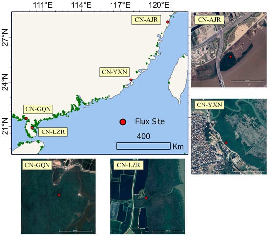
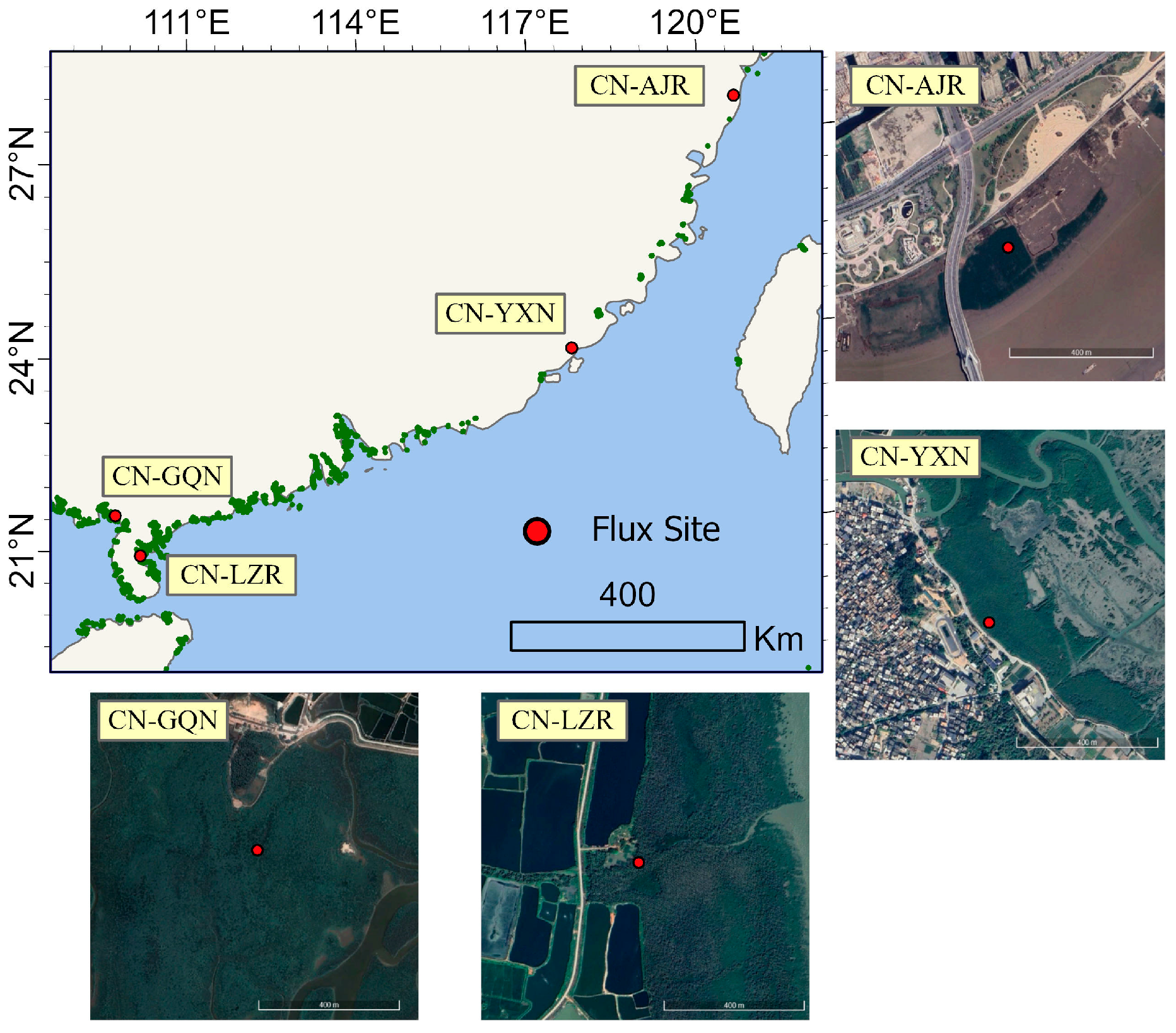
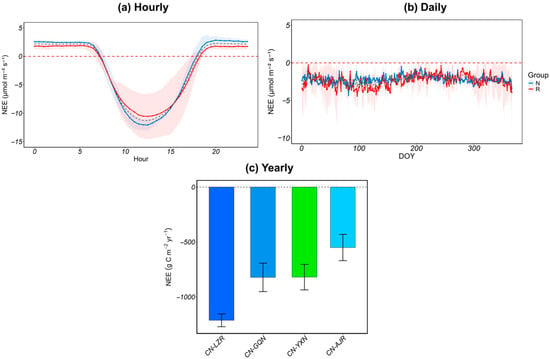
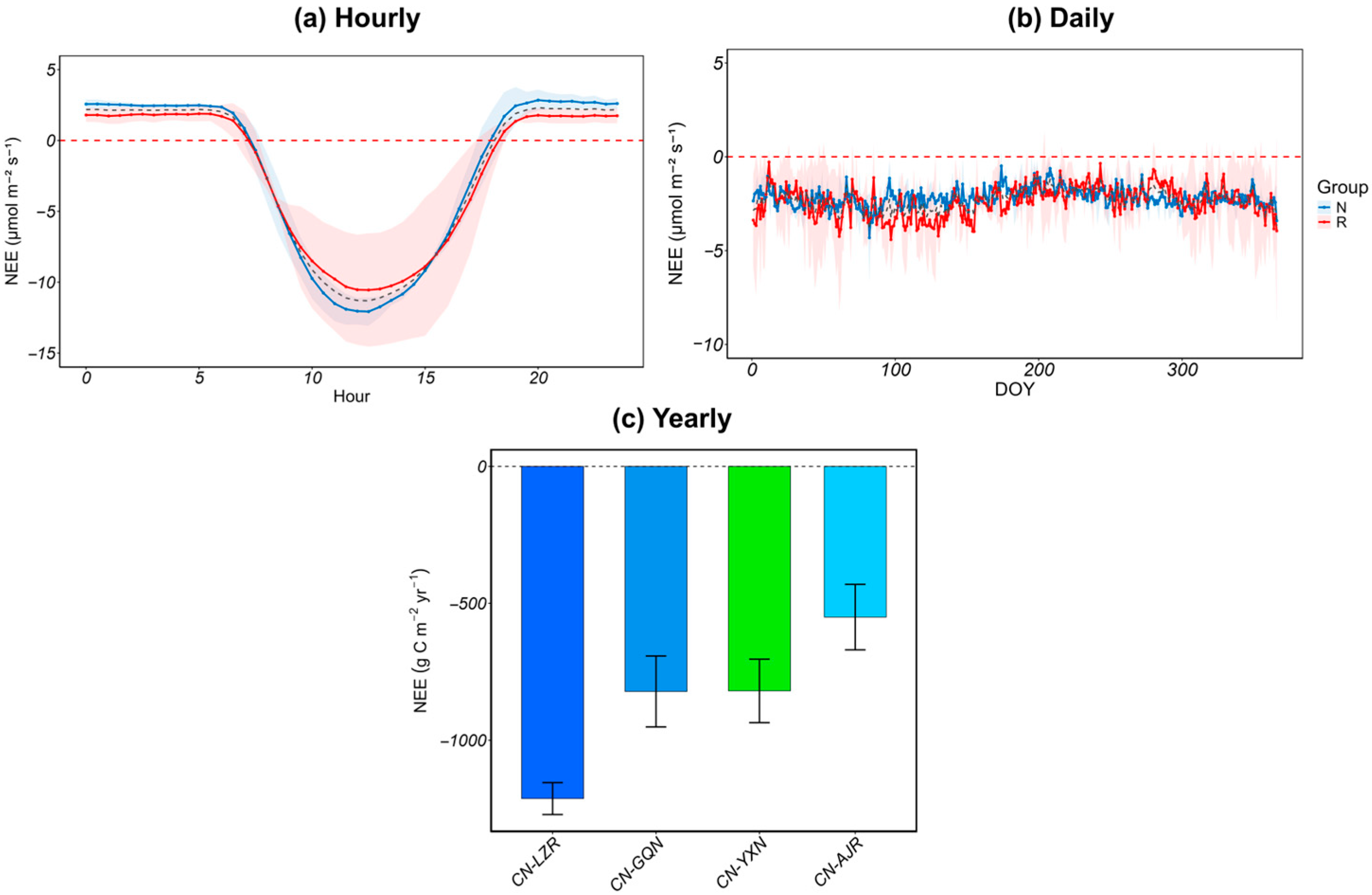
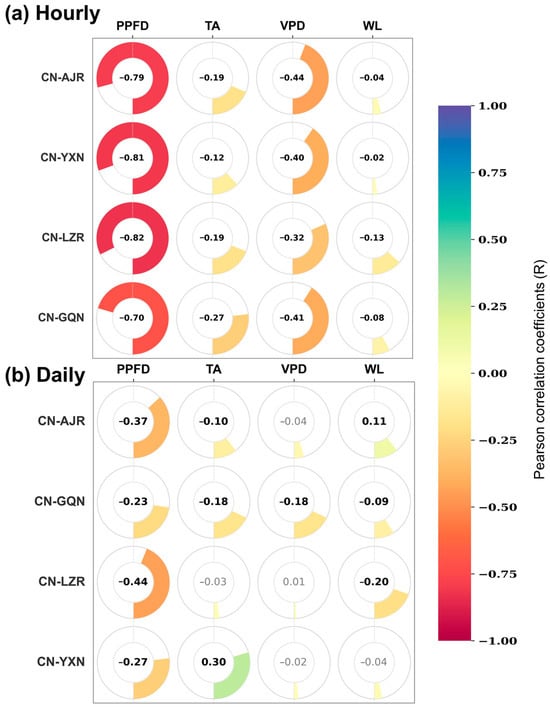
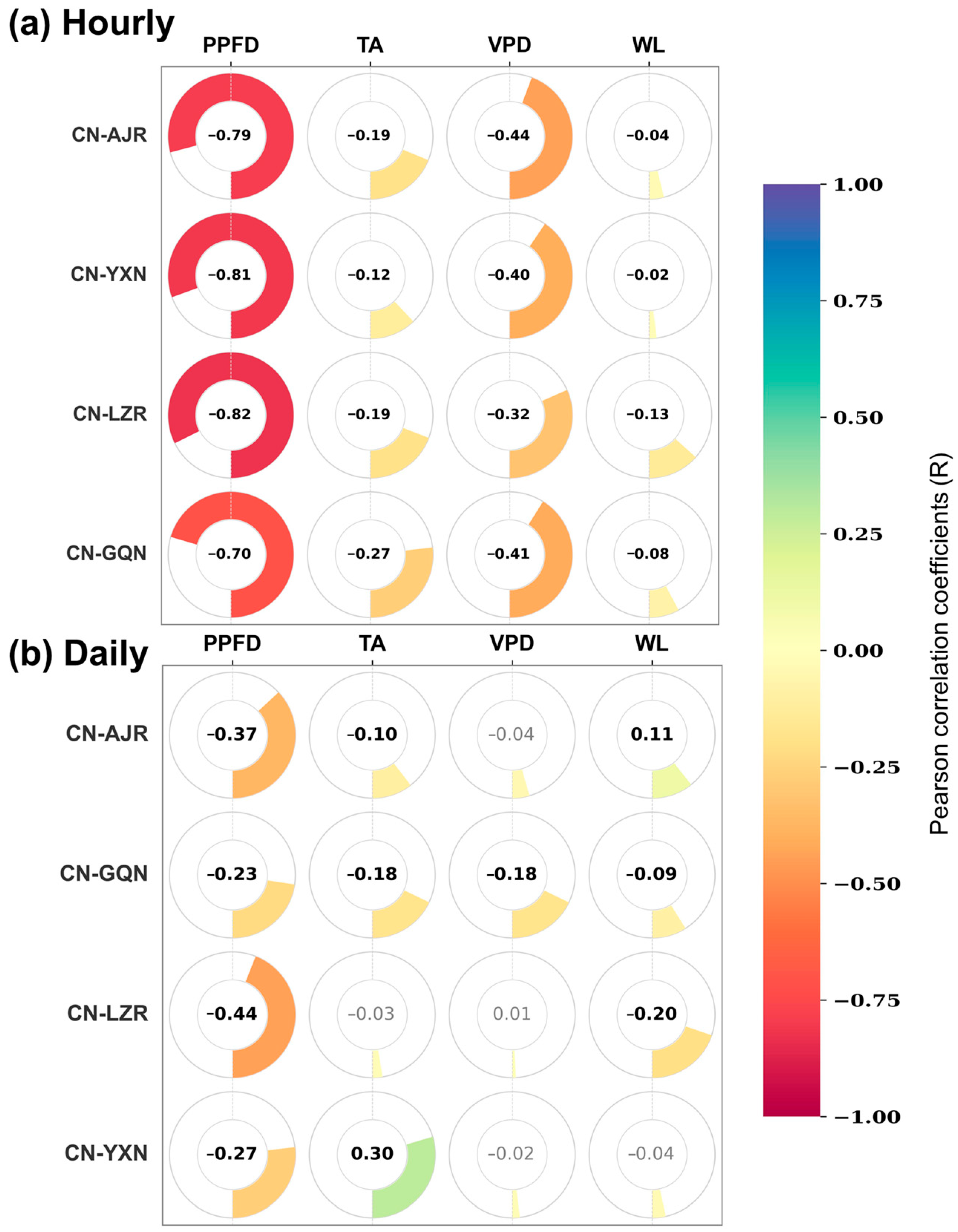
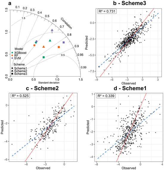
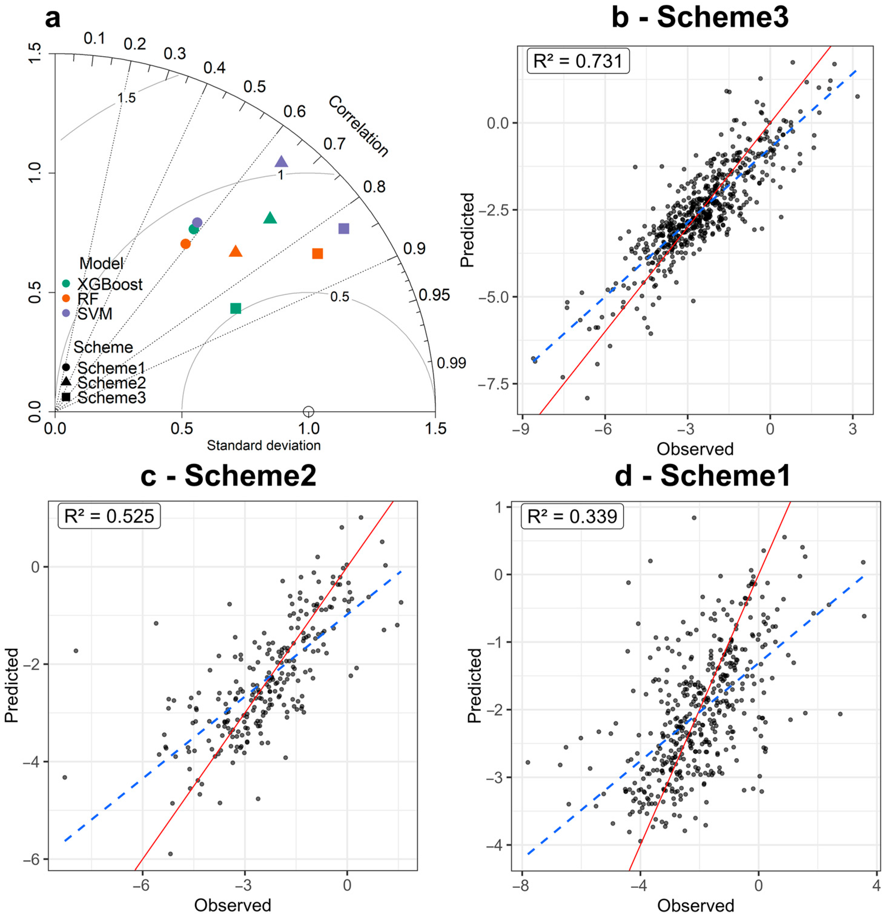
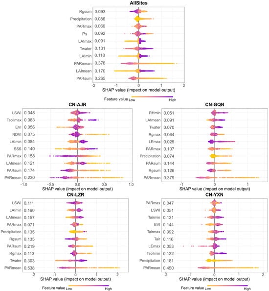
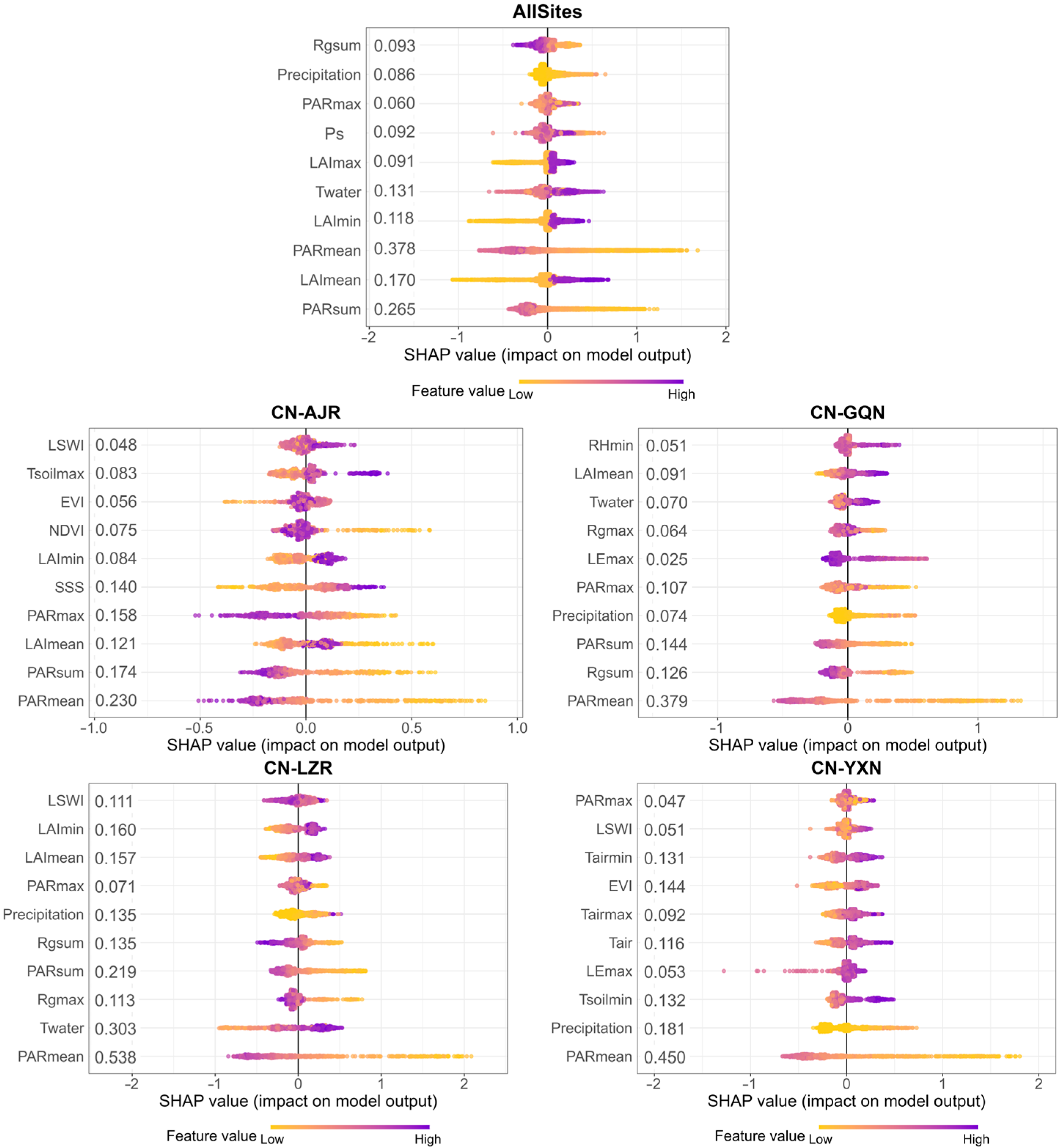
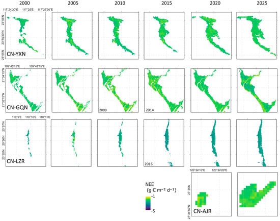
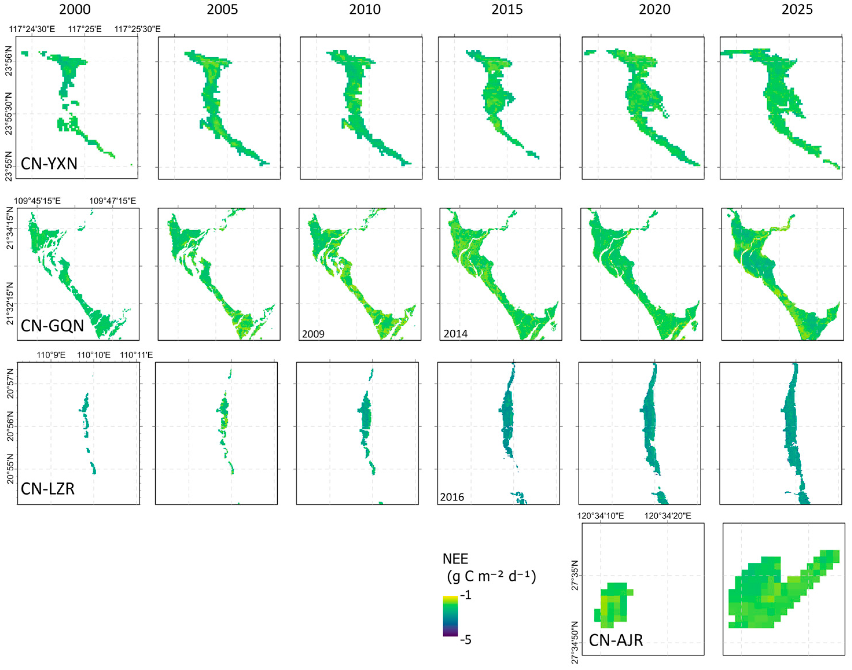

Disclaimer/Publisher’s Note: The statements, opinions and data contained in all publications are solely those of the individual author(s) and contributor(s) and not of MDPI and/or the editor(s). MDPI and/or the editor(s) disclaim responsibility for any injury to people or property resulting from any ideas, methods, instructions or products referred to in the content. |
© 2026 by the authors. Licensee MDPI, Basel, Switzerland. This article is an open access article distributed under the terms and conditions of the Creative Commons Attribution (CC BY) license.