Article

Using Multispectral UAV Imagery for Rye Biomass Estimation and SEM-Based Attribution Analysis

1
National Engineering Research Center for Geographic Information System, School of Geography and Information Engineering, China University of Geosciences, Wuhan 430074, China
2
Shenzhen Research Institute, China University of Geosciences, Shenzhen 518063, China
3
College of Agriculture, Ibaraki University, 3-21-1 Ami, Ibaraki 300-0393, Japan
*
Author to whom correspondence should be addressed.
Remote Sens. 2026, 18(4), 665; https://doi.org/10.3390/rs18040665
Submission received: 18 January 2026 / Revised: 11 February 2026 / Accepted: 17 February 2026 / Published: 22 February 2026
(This article belongs to the Special Issue Crop Yield Prediction Using Remote Sensing Techniques)

Highlights

What are the main findings?
  • UAV-derived canopy height is the strongest single predictor of rye dry biomass across the overall growth period, while selected vegetation indices perform best during the non-seedling stage.
  • Integrating canopy height, vegetation fraction, and vegetation indices in multi-parameter machine learning models yields consistently higher biomass estimation accuracy across growth stages, and SEM confirms their complementary direct and indirect effects on biomass accumulation.
What are the implications of the main findings?
  • Multi-temporal UAV multispectral remote sensing can support more reliable, stage-aware biomass monitoring for rye cover crops, enabling more informed management decisions in cash-crop systems.
  • Combining predictive machine learning with SEM-based attribution improves interpretability for remote-sensing biomass retrieval by linking spectral, structural, and fractional cover signals to mechanistic pathways of biomass accumulation.

Abstract

Effective management of rye cover crops in cash-crop systems relies heavily on accurate biomass estimation. Low-altitude Unmanned Aerial Vehicle (UAV) imagery offers a promising high-resolution alternative, yet unlocking its full potential requires moving beyond basic estimation models to more integrative and explanatory models. This study obtains the measured height (MH), SPAD (Soil and Plant Analyzer Development) values, and measured dry biomass (MDB) and applies UAV remote sensing and machine learning to acquire the crop canopy height, vegetation indices (VIs), and vegetation fraction (VF) across growth stages. Among single-parameter biomass estimation models, the estimated height yields the best at the overall growth stage (R2 = 0.935), whereas selected VIs perform the best at the non-seedling stage (R2 = 0.851). For multi-parameters modeling, models combining height, VF, and VIs significantly outperform the single-parameter models, achieving better estimation results throughout each growth stage (Best R2 = 0.951). Structural equation modeling clarifies the direct and indirect contributions of these parameters to biomass accumulation, revealing their synergistic effects. This study demonstrates the potential of UAV-based multi-parameter biomass estimation model to support more informed decisions in cover crop management and to advance broader precise agriculture practices. Additionally, the analytical framework developed here offers a transferable approach for high-resolution biomass monitoring in other crop systems.

1. Introduction

Estimating biomass accurately is crucial for managing cover crops, as it informs decisions related to soil health, erosion control, nutrient cycling, and subsequent economic crop growth [1,2]. Traditional ground-based sampling is labor-intensive and fails to capture field-scale spatial variability. Unmanned Aerial Vehicle (UAV) utilizes remote sensing technologies that can address these challenges. They provide a non-destructive, efficient, and precise methodology for quantifying biomass, enabling more effective and data-driven agricultural decisions [3].
Rye (Secale cereale L.) is widely used as a cover crop in agronomic practices due to its rapid growth, soil improvement capabilities, and weed suppression effects [4]. However, accurately estimating cover crop biomass remains a challenge due to its varying growth patterns across different developmental stages. Previous studies have applied remote sensing to estimate biomass. Baraibar et al. predict weed biomass using accumulated cover-crop-growing degree days [5] and crop type. Kharel et al. estimate biomass of mixed cover crops using high-resolution satellite imagery [6]. These studies have developed models for cover crops using imaging technology, demonstrating that remote sensing can be effectively used to provide a biomass estimation.
Crop height can be monitored via UAV photogrammetry, which acquires high-resolution three-dimensional point clouds to enable precise canopy height measurements [7]. UAV-derived height measurements have shown a strong linear relationship with actual crop height, which is in turn associated with biomass. Crop phenotyping studies based on multispectral and hyperspectral technologies have shown that vegetation indices (VIs) are related to specific morphological and physiological parameters [1,8]. Multispectral or hyperspectral camera sensors mounted on UAVs enable the calculation of VIs. UAV platforms have proven effective in estimating crop height and biomass across different crops, including rice [9], sweet corn [10], and wheat [11]. However, models that estimate biomass using only VIs often lack accuracy [12,13]. Research shows that biomass models based on plant height, or a combination of height and VIs, generally achieve a better correlation than those relying on VIs alone [9,14]. Furthermore, recent studies have demonstrated that incorporating structural and textural information can, to some extent, alleviate the saturation of spectral features during the reproductive growth stage and improve biomass inversion performance in the mid-to-late growth periods [15]. In addition, integrating environmental and management factors, such as topography and planting structure (e.g., planting density and row spacing), with VIs can significantly enhance the model’s adaptability to spatially heterogeneous fields and its generalization capability [16,17].
Nonetheless, some studies report that adding plant height data to multiple linear regression models based on vegetation indices does not significantly enhance biomass estimation performance [18]. The combination of UAV-based multispectral data and textural features has also been demonstrated to provide notable gains in the estimation of rice aboveground biomass [19]. In recent years, an increasing number of studies have adopted multi-source feature fusion and ensemble learning frameworks to improve the consistency and robustness of biomass estimation across multiple growth stages for rice and other crops [20]. However, most studies have not further investigated the internal structure and interpretability of their estimation models, nor thoroughly assessed the individual contributions of each estimator to the overall biomass estimation. Effective management of cover crops like rye requires accurate biomass estimation, yet conventional remote sensing approaches often stop at estimation modeling—such as identifying optimal VIs, developing robust UAV-based crop height estimation models, and introducing canopy structure parameters (e.g., vegetation fraction (VF))—without providing deeper insights into the agronomic drivers. This limitation hinders the model’s interpretability and transferability. To address this gap, this study proposes a novel analytical framework that not only develops a robust UAV-based crop height and multi-parameter estimation model, but also conducts a critical attribution analysis to understand the model’s performance. To facilitate this analysis, structural equation modeling (SEM) is applied to disentangle the latent drivers of biomass—capturing both direct and indirect pathways while explicitly modeling measurement error.
This study aims to design a multi-parameter rye biomass estimation method based on UAV multi-temporal multispectral imagery. On this basis, an attribution approach is also proposed. The specific objectives within this framework are:
(1) To evaluate the relationship between ground-measured crop height and UAV-derived crop height models across the seedling, non-seedling, and overall growth stages. This will determine the extent to which UAV measurements can accurately reflect crop height variations at different developmental stages.
(2) To analyze the estimation capability of various VIs and VF in estimating the relative chlorophyll content. We explore the effectiveness of different combinations of VIs on ground-based measurements of SPAD (Soil and Plant Analyzer Development) data.
(3) To develop single-parameter and multi-parameter biomass estimation models using height, VIs, VF, and their combination. These models aim to estimate biomass by capturing the complex relationships between these parameters, utilizing k-fold cross-validation to ensure model reliability.
(4) To further analyze the parameter contribution of the proposed biomass estimation framework, the categorized parameters are then analyzed using SEM.
Therefore, the primary scientific objectives of this study are to establish a high-performance biomass estimation model by integrating UAV-derived metrics (height, VIs, and VF) and, more critically, to innovate the attribution analysis process through SEM. By shifting the analytical focus from simple prediction to the elucidation of causal pathways, this study aims to enhance the interpretability of biomass accumulation dynamics. Ultimately, we seek to provide a transferable, integrated framework that combines high-resolution sensing with mechanistic modeling for advanced agronomic monitoring.

2. Datasets

2.1. Experimental Design

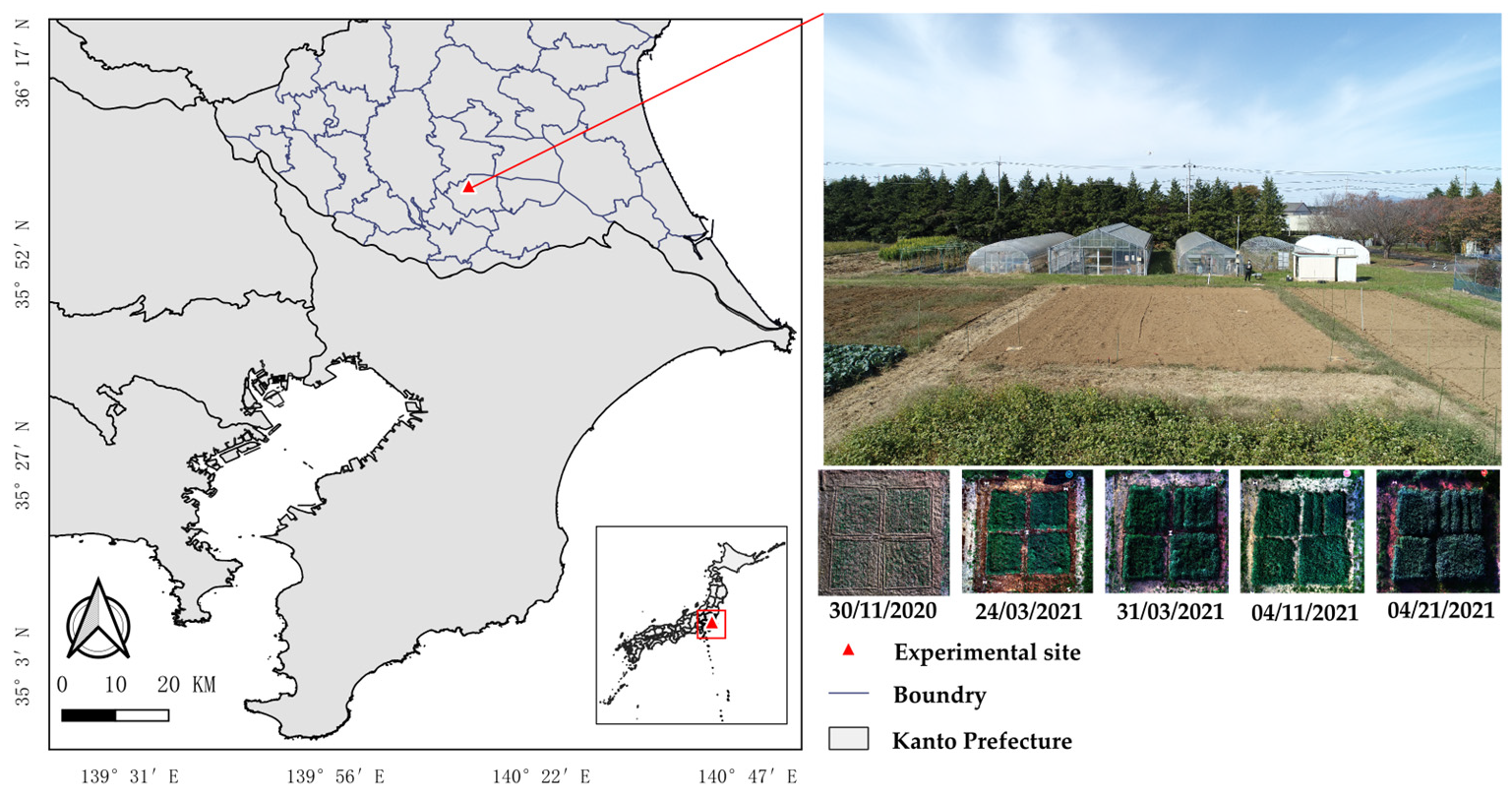
The research was conducted at the International Research and Education Center for Field Agriculture, Ibaraki University, located in Ibaraki Prefecture, Japan (36°01′56.9″ N 140°12′41.2″ E; Figure 1). The region has a humid temperate monsoon climate, and the soils are predominantly Andosols of volcanic ash origin. During the experimental period (November 2021 to May 2022), the mean air temperature was 9.1 °C and the total precipitation was 730.5 mm, based on monthly records from the Japan Meteorological Agency’s Tsukuba (Tateno) station. The study site, lying fallow following an upland rice harvest, was established within a rye field.
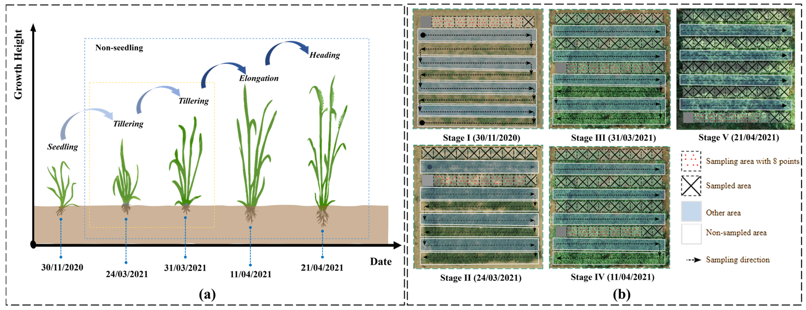
To assess biomass dynamics throughout the growth cycle, on-site measurements were collected at key developmental stages. These measurements included the SPAD (Soil and Plant Analyzer Development) value of canopy leaves, measured height (MH), and regional measured dry biomass (MDB). Biomass sampling was conducted within a demarcated 50 cm × 50 cm quadrat, which served as the sampling zone. Critical sampling dates and their corresponding growth stages are summarized in Table 1: 3 December 2020 (seedling stage); 24 and 31 March 2021 and 11 April 2021 (representing tillering and elongation stages); and 21 April 2021 (heading stage). The sampling stages (divided into seedling and non-seedling stages for analysis) and the sampling pattern are shown in Figure 2a and Figure 2b, respectively.

2.2. UAV Flights

Aerial multispectral imagery was acquired using a Phantom 4 Multispectral (P4M) UAV equipped with an FC6360 camera (DJI, Shenzhen, China). Flights were executed during suitable weather windows within the daytime periods corresponding to the on-site sampling. The FC6360 integrates five narrow-band multispectral sensors covering blue (450 nm ± 16 nm), green (560 nm ± 16 nm), red (650 nm ± 16 nm), red edge (730 nm ± 16 nm), and near-infrared (NIR, 840 nm ± 26 nm) wavelengths, alongside a panchromatic RGB sensor. These six sensors are physically arranged in a 2 × 3 configuration. Crucially, the optical centers of all sensors are precisely calibrated relative to the phase center of the onboard D-RTK GNSS antenna on the P4M, ensuring high geolocation accuracy. The camera captures imagery in a tagged image file format with a digital number range of 0 to 65,535, utilizing 1/2.9 inch CMOS sensors for all bands. Detailed parameters for each UAV flight mission, including date, altitude, solar angles (azimuth/altitude), sensor information, number of images/composites, and the resulting ground sampling distance, are comprehensively documented in Table 1.

3. Frameworks

3.1. UAV Image Preprocessing Process

The P4M UAV’s camera captures reflected light, while its integrated sunshine sensor corrects for ambient light variations, ensuring data are comparable across different growth stages [21]. The pre-processing mainly consists of radiometric calibration, geometric distortion correction, multi-band image position correction, and bidirectional reflectance calculation of images.
Radiometric calibration aims to eliminate sensor inherent biases and environmental lighting variations [22], including black level correction (BLC), exposure and gain correction (EGC), lens shading correction (ISC), relative spectral radiance calculation (rSRC) (Figure A1a). The BLC equation is shown:
V 1 ( u ,   v )   =   V ori ( u ,   v ) D N blackcurrent
where V ori ( u ,   v )   and D N blackcurrent are pixel coordinates and black level value at digital number (DN), respectively. The EGC equation is shown:
V 2 ( u ,   v )   =   V 1 ( u , v ) g sensor · t exposure 10 6
where g sensor is the gain of the camera sensor, t exposure is the time of exposure, and V 2 is the DN value with EGC. Equation (3) is applied to correct edge brightness fall-off (lens shading).
V 3 ( u ,   v ) = V 2 ( u ,   v ) · ( k 5 · r 6 + k 4 · r 5 + k 3 · r 4 + k 2 · r 3 + k 1 · r 2 + k 0 · r + 1 )
where r = ( u - u center ) 2 + ( v - v center ) 2 is the radial distance from the image center   ( u center ,   v center ) to a given pixel ( u ,   v ) and k i ( i   =   1 ,   2 ,   5 ) are vignetting polynomial coefficients. rSRC is then calculated using the following:
L ( u , v ) = ( k 5 r 6 + k 4 r 5 + k 3 r 4 + k 2 r 3 + k 1 r 2 + k 0 r + 1 ) × ρ × V 3 ( u , v ) p B L g sensor × t e x p o s u r e
where p B L is the background brightness of the sensor when the shutter is closed and ρ is the correction of the light intensity sensitivity of the band sensor, with respect to the NIR band.
Geometric distortion correction eliminates lens and sensor aberrations to ensure the geometric fidelity of images. We utilized a computational correction method based on pre-calibrated intrinsic parameters derived from the Brown–Conrady distortion model to rectify image distortion (Figure A1b). The undistorted coordinates are calculated by the following:
x undistorted   =   x ( 1 + k 1 r 2 + k 2 r 4 + k 3 r 6 + k 4 · r 8 ) + 2 p 1 xy + p 2 ( r 2 + 2 x 2 ) y undistorted   =   y ( 1 + k 1 r 2 + k 2 r 4 + k 3 r 6 + k 4 · r 8 ) + p 1 ( r 2 + 2 y 2 ) + 2 p 2 xy
where r = ( x - x center ) 2 + ( y - y center ) 2   is the squared radial distance from the center of the image, and k i ( i   =   1 4 ) and p j ( j   =   1 ,   2 ) are radial distortion coefficients and tangential distortion coefficients, respectively.
Positional shifts between bands, caused by the physical separation of sensors and minor differences in exposure times, are corrected by aligning all bands to the radiometric reference NIR band. This translation is defined as follows:
u trans = u ori u relative v trans = v ori v relative
where ( u ori ,   v ori ) and ( u trans ,   v trans ) are original and translated pixel coordinates, respectively, and u relative and v relative are relative offsets. We registered the visible and red-edge bands to the NIR band using feature extraction, robust matching, and geometric transformation to achieve accurate multispectral alignment (Figure A1c). We calculated the desired vegetation indices (VIs) after completing the above. Since absolute reflectance calibration using a reference panel is not performed, bidirectional reflectance factors cannot be derived. Instead, VIs can be calculated directly from the relative spectral radiance values.

3.2. Crop Height Model

We used nadir photogrammetry to maximize canopy point density in sparse rye canopies. A crop height model (CHM) was generated from 3D point clouds reconstructed from multi-temporal UAV imagery. Each point contained precise 3D coordinates (latitude, longitude, and ellipsoidal height in WGS84/UTM zone 54N) and calibrated spectral radiance data. To achieve canopy point cloud selection, we firstly calculated the normalized difference vegetation index (NDVI) at various growth stages (seedling stage, tillering stage, elongation stage and heading stage), as follows:
P C NDVI   =   P C NIR P C Red P C NIR + P C Red
where P C N D V I is the resulting NDVI value, and P C R e d and P C N I R are the red and near-infrared reflectance values derived from the point cloud. Then, an adaptive thresholding technique was applied using Otsu’s method. This algorithm automatically determines an optimal threshold T by segmenting the P C N D V I values into two classes: vegetated and non-vegetated classes. The objective function is defined as follows:
max T   [ σ B 2 ( T ) = w 1 ( T ) · w 2 ( T ) · ( μ 1 ( T ) - μ 2 ( T ) ) 2 ]
where w 1 ( T ) and w 2 ( T ) are the weights of the vegetation and non-vegetation classes, respectively, and μ 1 ( T ) and μ 2 ( T ) are the mean NDVI values for each class. At each growth stage, the Otsu’s method was applied to each 50 × 50 cm sampling region of interest (ROI) to determine the corresponding threshold T j . For the j-th ROI, points whose NDVI values are above the corresponding threshold T j are classified as a canopy called P C selected ,   j , as shown:
P C selected ,   j   =   { P C NDVI ,   j | P C NDVI ,   j > T j }
Across all ROIs, the automatically determined thresholds derived from the algorithm range from 0.29 to 0.35. This range is physically reasonable, as non-vegetation classes (primarily bare soil) typically exhibit lower NDVI values (approximately 0.18–0.26), whereas vegetation classes generally show higher NDVI values [23,24,25]. To calculate CHM, we used the ellipsoidal height of the point cloud at the germination stage as a topographic reference, and the ellipsoidal height of the other stages as calculation objects, with the following:
H canopy   =   h ellipsoid , t i h ellipsoid , t 0 + ϵ
where h e l l i p s o i d ,   t 0 is the ellipsoidal height at a reference stage, h e l i p s o i d , t i , is the ellipsoidal height at other growth stages, and ϵ represents potential system error and measurement noise.
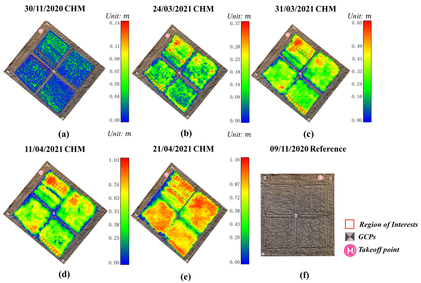
We used QGIS 3. 12 to plot Shapefiles as ROIs which are 50   c m   ×   50   cm areas, matching the field survey sampling area, as shown in Figure 3. We used CloudCompare 2.12 to estimate the canopy height of each ROI, which are divided into equal-sized grids of 0.01 × 0.01 m. The estimated height (EH) of the canopy of each ROI is defined as follows:
EH canopy ( ROI ) = 1 n i = 1 n   D max ,   i
where D m a x ,   i represents the maximum difference value within each grid cell, and n is the total number of grid cells (typically 2500).

3.3. Orthophoto Map Generation, Canopy Masking, and Vegetation Index Calculation

Orthomosaic processing removes geometric distortions from an image to ensure consistent and accurate measurements, allowing all regions to be reliably compared. Following pre-processing in Section 3.1, we imported image sets into Pix4Dfields 1.9 software to generate orthophoto maps (Figure A2a). At each crop growth stage, the image data includes five single-channel grayscale orthophotos (blue, green, red, red edge, and near-infrared) and a panchromatic orthophoto created by fusing the blue, green, and red data.
Accurately extracting crops requires separating them from non-crop areas. While simple color filtering is one method, its results are often biased by changes in brightness. We adopted a more robust approach based on the normalized difference vegetation index (NDVI). A classification mask can be created by thresholding the NDVI image with algorithms like the Otsu method [26] or K-means [27,28]. However, this approach struggles to distinguish crops from other unwanted vegetation. This study evaluated four algorithms—random forest (RF) [29], support vector machine (SVM) [30], artificial neural network based on genetic algorithm (ANN-GA) [31], and K-nearest neighbor (KNN) [32]—to determine the best method for generating crop masks from the panchromatic orthophoto map (Figure A2b). Furthermore, we constructed our dataset by randomly sampling 70% of the pixels for training and reserving 30% for independent testing. Hyperparameters were selected via grid search using five-fold cross-validation (CV) on the training subset only. Specifically, for each candidate hyperparameter combination (Table A1), models were trained on four folds and validated on the remaining fold; performance was averaged across folds, and the best configuration was chosen by maximizing the mean CV score. The independent test set was kept untouched during model selection and was used only for the final evaluation.
For RF, the grid search was conducted over the number of trees, maximum tree depth, and minimum leaf size, and the final model used 100 trees, a maximum depth of 25, and a minimum of five samples per leaf. For SVM, we used an RBF kernel and tuned the penalty parameter C of 1.0 and kernel width γ of two. We scaled all input bands to zero mean and unit variance before training to ensure stable convergence of the quadratic optimizer. For ANN-GA, a feed-forward neural network of two hidden layers was adopted. The final setting used 32 and 16 neurons in the two hidden layers, a population size of eight, four parents per generation, 100 generations, and a mutation rate of 10%. The optimization objective was to minimize categorical cross-entropy loss on the training set, and early stopping was applied when the validation loss plateaued. For KNN, the distance metric and weighting scheme were tuned by grid search. The final model classified each pixel by a majority vote among the k nearest neighbors in a spectral feature space, using Euclidean distance. The generated mask was applied to the single-channel grayscale image, allowing us to extract the 50 × 50 cm ROI with the Shapefile from Section 3.2 to calculate the relevant index (Figure A2c).
Based on the primary biophysical parameters they are designed to estimate, vegetation indices are classified into categories related to nitrogen accumulation, chlorophyll content, and canopy health. Nitrogen accumulation is strongly correlated with 760 nm, 810 nm, and 870 nm [33]. For rice and wheat, the nitrogen index (NI) developed by Tian et al. shows good correlation with leaf N accumulation [34,35] and is related to the 715 nm, 705 nm, and 491 nm bands; therefore, we used NI (red edge, blue) as the nitrogen accumulation vegetation index. Previous studies show a close relationship between chlorophyll content and the biomass of gramineous cereal crops [36,37]. Several vegetation indices can reflect the chlorophyll content and its changes by combining different wavelength bands. The green normalized difference vegetation index (GNDVI), using the 800 nm and 550 nm bands, is highly sensitive to both the absolute values and changes in chlorophyll [38]. The optimized soil adjusted vegetation index (OSAVI), using the 800 nm and 670 nm bands, more accurately reflects the absolute chlorophyll value by optimizing for different soil backgrounds [39]. The spectral polygon vegetation index (SPVI), combining the 800 nm, 670 nm, and 530 nm bands, can sensitively capture chlorophyll changes [40]. Therefore, we used GNDVI (near-infrared, green), OSAVI (near-infrared, red), and SPVI (near-infrared, red, green) as chlorophyll content vegetation indices. Photosynthetic capacity is one of the core indicators of vegetation health. The normalized difference vegetation index (NDVI) is a well-recognized measure of the photosynthetic capacity of vegetation [41]. The renormalized difference vegetation index (RDVI) combines the 840 nm and 650 nm bands and is more sensitive to low-cover vegetation [42,43]; studies show that RDVI is more sensitive to changes in photosynthetic capacity [44]. The ratio vegetation index (RVI), defined as the ratio of reflectance between the 670 nm and 840 nm bands, is one of the earliest vegetation indices used to assess vegetation health; it does not tend to saturate easily, is suitable for analyzing intensive crops, and responds faster under large health changes [45]. Therefore, we used NDVI (near-infrared, red), RDVI (near-infrared, red), and RVI (near-infrared, red) as canopy health vegetation indices. The mathematical equations for these indices, adapted for the five spectral bands of the P4M UAV, are detailed in Table 2.

3.4. Statistical Analysis Methods

We applied Ordinary Least Squares (OLS) regression to examine the relationships among field-measured height, UAV-derived canopy height model (CHM), and dry biomass, estimating coefficients by minimizing the sum of squared errors. The OLS model is as follows:
β ^   =   ( X T X ) 1 X T Y
where β ^ is the estimate of the regression coefficient, X is the matrix of independent variables, Y is the vector of dependent variables, X T is the transpose matrix of X , and ( X T X ) 1 is the inverse matrix of X T X . This formula represents the solution of the optimal regression coefficient β ^ by minimizing the sum of squares of the residuals.
As SPAD (Soil and Plant Analyzer Development) and biomass are influenced by multiple variables, feature selection is needed to reduce multicollinearity and overfitting [46]. Best subset regression (BSR) is computationally expensive and relies on repeated OLS fits, making it vulnerable to these issues [47]. Ridge regression mitigates multicollinearity via coefficient shrinkage but cannot perform true feature selection [48]. Therefore, we adopted the least absolute shrinkage and selection operator (LASSO), which uses L1 regularization to enable sparse selection [49], as follows:
β ^ = arg min β   { 1 2 n i = 1 n   ( y i - x i T β ) 2 + λ j = 1 p   | β j | }
where β ^ is the estimated value of the regression coefficient, n is the number of samples, ( y i ,   x i ) is the i observed sample, and λ is the regularization parameter, which controls the complexity of the model. LASSO regression can reduce the coefficients of unimportant variables to zero by adding the L1 regularization term ( j = 1 p   | β j | ) to the objective function, thereby effectively removing these variables from the model, performing feature selection and simplifying the model. Model complexity is reduced after LASSO regression feature selection and leave-one-out cross validation is applied to evaluate the scores.
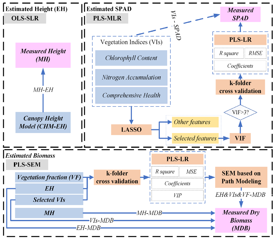
We used a combined LASSO and partial least squares regression (PLSR) approach to model measured SPAD and biomass. PLSR mitigated multicollinearity by extracting latent variables [50,51] and was suitable for small sample sizes. The number of latent variables was optimized via k-fold cross-validation to limit overfitting, and variable importance in projection (VIP) scores were used to identify influential predictors. When multicollinearity persisted after LASSO, PLSR was applied. The matrix of regression coefficients, B c , is calculated from dependent variable Y v , using the following:
B c = ( P sel T W opt ) 1 S sel T   Y v
where S s e l T is the selected potential structure matrix, P s e l T is the selected loading matrix, and W o p t is the optimized weight matrix. We employed structural equation modeling (SEM) to estimate biomass from CHM, three vegetation-index groups, and vegetation-fraction scores while jointly quantifying their relationships. We adopted partial least squares path modeling (PLS-PM) instead of covariance-based SEM because it is prediction-oriented and robust to small sample sizes and non-normal data [52,53,54]. We specified both a measurement model and a structural model; the measurement model is expressed as follows:
{ X o b s = Λ x , p ξ e x + δ Y o b s = Λ y , p η e n + ε
where links observe data ( X o b s , Y o b s ) to exogenous ( ξ e x ) and endogenous ( η e n ) latent variables via loading matrices ( Λ x , p , Λ y , p ), with measurement errors ( δ , ε ). The structural model is expressed as follows:
η e n = B e n d o η e n + Γ e x o ξ e x + ζ s t r u c t
where Γ e x o represents the effect of exogenous variables on endogenous variables, B e n d o represents the relationships among endogenous variables, and ζ s t r u c t is the structural error. The overall statistical analysis framework employed for multi-source data is depicted in Figure 4.

4. Results

4.1. Optimal Crop Mask Algorithm

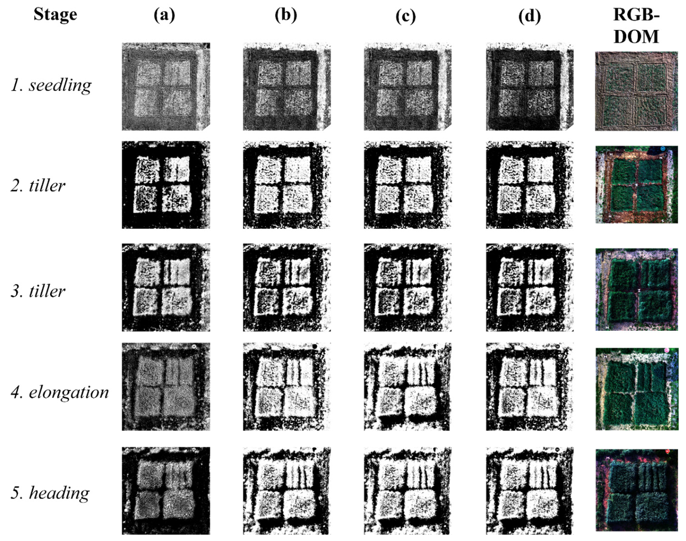
Four supervised learning algorithms—random forest (RF), support vector machine (SVM), artificial neural network based on genetic algorithm (ANN-GA), and K-nearest neighbors (KNNs)—were systematically evaluated for their performance in classifying vegetated and non-vegetated areas, based on a multispectral orthomosaic map (Figure 5). Each algorithm was assessed on its ability to generate crop-specific masks.
The experimental results (Table 3) indicate that the RF algorithm exhibits the best performance across all evaluation metrics among the tested models. RF achieves the highest classification accuracy, significantly reducing misclassification of background elements and non-target vegetation compared to the other methods. This can be attributed to RF’s ability to handle high-dimensional data and its inherent capacity for modeling complex decision boundaries, making it well-suited for remote sensing applications involving vegetation.

4.2. Height Estimation Using Measured Height and Estimated Height

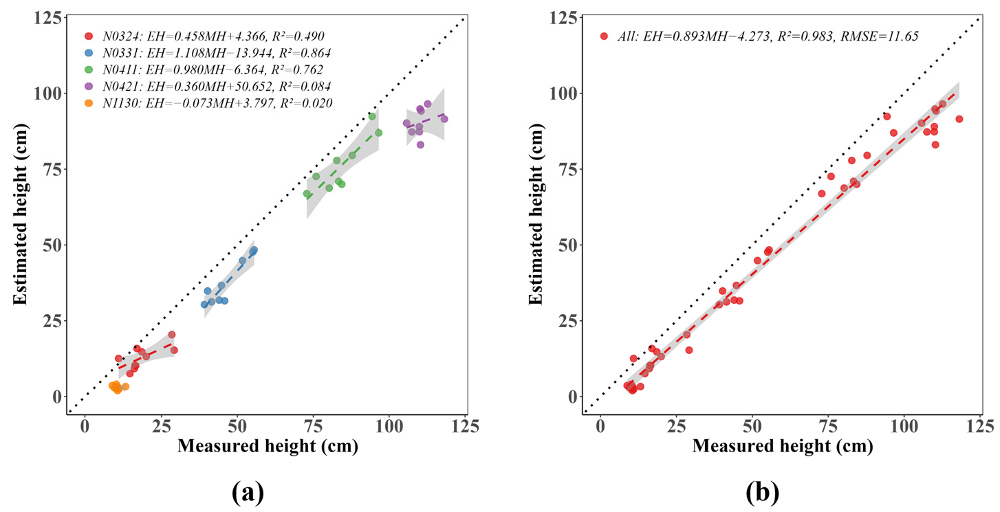
The relationship between measured height (MH) in the field and estimated height (EH) derived by UAV photogrammetry is linearly comparable. As shown in Figure 6a, we used OLS linear regression to build model across different dates. Figure 6b shows the model built using data from all dates as an overall growth stage.
Performance varies considerably by growth stage. The weakest correlations occur at the seedling stage (N1130, R2 = 0.02) and the heading stage (N0421, R2 = 0.084). In contrast, the tiller and stem extension stages (N0324–N0411) exhibit substantially stronger correlations (R2 = 0.490~0.864), with the highest observed at N0411 (R2 = 0.864). Considering the overall growth stage, MH and EH demonstrate excellent linear agreement, yielding an R2 of 0.983 and an RMSE of 11.65 cm.

4.3. SPAD Estimation Using Vegetation Indices

The SPAD (Soil and Plant Analyzer Development) value is highly correlated with the relative chlorophyll content per unit area [55], which is a basic physiological indicator of rye growth. The SPAD values are obtained by calculating leaf transmittance at 650 nm in the spectrum, a wavelength absorbed by chlorophyll, and at 940 nm in the near-infrared (NIR) spectrum [56,57]. Given that the P4M UAV mounted multispectral camera used in this study does not capture wavelengths greater than 900 nm in the NIR spectrum, this research focused on estimating SPAD values (as a proxy for relative chlorophyll content) using vegetation indices (VIs), which are explained in Section 3.4. Feature selection is performed using the LASSO method. Subsequently, an OLS multiple linear regression model (MLR) of the selected features, including GNDVI, OSAVI, SPVI, and NDVI, is built.
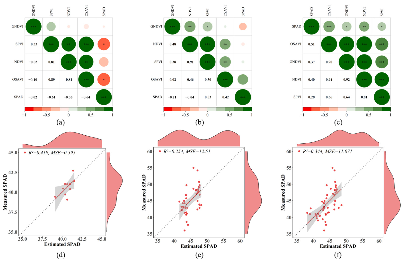
At the seedling stage, the correlation matrix reveals no significant association between SPAD and GNDVI ( r   =   0.02 ) (Figure 7a). SPAD exhibits a weak negative correlation with NDVI ( r   =   0.35 ), and moderate negative correlations with OSAVI ( r   =   0.64 * ) and SPVI ( r = 0.61 * ). Consequently, OSAVI and SPVI are selected as the primary estimators in the SPAD estimation model. This model yields an R2 of 0.419, with an RMSE of 0.77 (Figure 7d), indicating moderate model performance during the seedling stage. At the non-seedling stage, correlations between SPAD and VIs are generally weaker (Figure 7b). SPAD exhibits a negligible correlation with NDVI ( r = 0.04 ) and GNDVI ( r = 0.21 ), while OSAVI shows a modest positive correlation ( r = 0.42 ). NDVI and OSAVI are selected as estimators for an MLR model, achieving an R2 of 0.254 and an RMSE of 3.54 (Figure 7e), reflecting limited model performance in the non-seedling growth stage.
During the overall growth stage, a moderate correlation was observed between SPAD and OSAVI ( r = 0.51 * * * ), with modest correlations detected for SPVI ( r = 0.28 ), GNDVI ( r = 0.37 ), and NDVI ( r = 0.40 ) (Figure 7c). Consequently, OSAVI, NDVI, and SPVI were selected as estimators for an MLR model, yielding an R2 of 0.344 and an RMSE of 3.33 (Figure 7f). Although estimation performance at the overall growth stage is weaker than during the seedling stage, it remains superior to that of the non-seedling stage.

4.4. Single Parameter Estimation of Measured Dry Biomass

We conducted experiments to evaluate the relationship between crop height and dry biomass at various stages, aiming to assess the effectiveness of only height in biomass estimation.
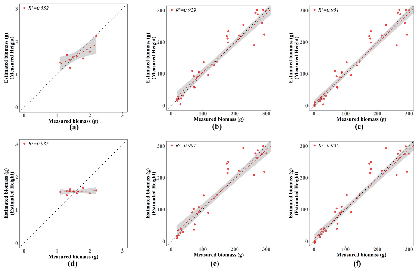
At the seedling stage, as shown in Figure 8a, the relationship between the measured height (MH) and measured dry biomass (MDB) exhibits a moderate linear correlation, with an R2 of 0.552. This suggests that the MH serves as a reasonable estimator for MDB at early rye growth. However, when biomass is estimated using the estimated height (EH), the model shows a week linear relationship (R2 = 0.035) (Figure 8d), indicating that the EH may not be accurately obtained by UAV Photogrammetry at this growth stage. At the non-seedling stage, the relationship between the MH and the MDB is significantly improved. As depicted in Figure 8b, the model yields an R2 of 0.929, demonstrating a robust linear relationship. The EH also shows a strong linear relationship with the MDB, with an R2 of 0.907 (Figure 8e). This suggests that as the rye develop and increase in height, UAV-based height estimation becomes more accurate for biomass estimation. During the overall growth stage, both the MH and EH perform well in estimating biomass. As depicted in Figure 8c, the model shows a strong linear relationship between MH and MDB, with an R2 of 0.951, and also, a robust linear relationship between EH and MDB, with an R2 of 0.935 (Figure 8f).
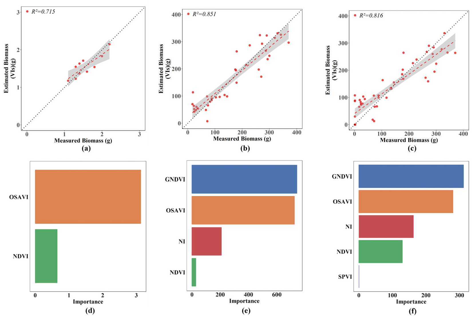
VIs mentioned in Section 3.4 were evaluated to determine their relationship with MDB. An exploratory analysis was performed to select the most relevant parameters for biomass estimation, using the LASSO method (Table 4). Subsequently, PLSR was applied to the selected parameters to build the model. At the seedling stage, the model used OSAVI and NDVI achieves an R2 of 0.715, as shown in Figure 9a. Variable Importance in Projection (VIP) analysis (Figure 9d) indicates that OSAVI contributes the most to the model. At the non-seedling stage, the model using GNDVI, OSAVI, NI and NDVI shows a stronger performance compared to the seedling stage, achieving an R2 of 0.851, as shown in Figure 9b. VIP analysis (Figure 9e) indicates that GNDVI is the most influential estimator, followed by OSAVI. During the overall growth stage, the model using GNDVI, OSAVI, NI, NDVI, and SPVI achieves an R2 of 0.816, as shown in Figure 9c. VIP analysis (Figure 9f) indicates that GNDVI and OSAVI contribute the most to the model.
All the models yielded R2 values exceeding 0.7, and the p-values for all models are <0.001, indicating that the established PLSR model is statistically reasonable. These results suggest potential for using canopy VIs to estimate biomass accurately throughout the rye growth cycle.

4.5. Combined Parameters to Dry Biomass Estimation

Building on our single-parameter findings in Section 4.4, we investigated the combined impact of the estimated height (EH), vegetation indices (VIs), and the structural parameter vegetation fraction (VF) on rye dry biomass estimation. Dry crop biomass accumulates over the growing period, and crop height likewise increases over time, whereas VIs and SPAD readings capture only the canopy’s instantaneous status. However, VF partially reflects canopy cover dynamics.
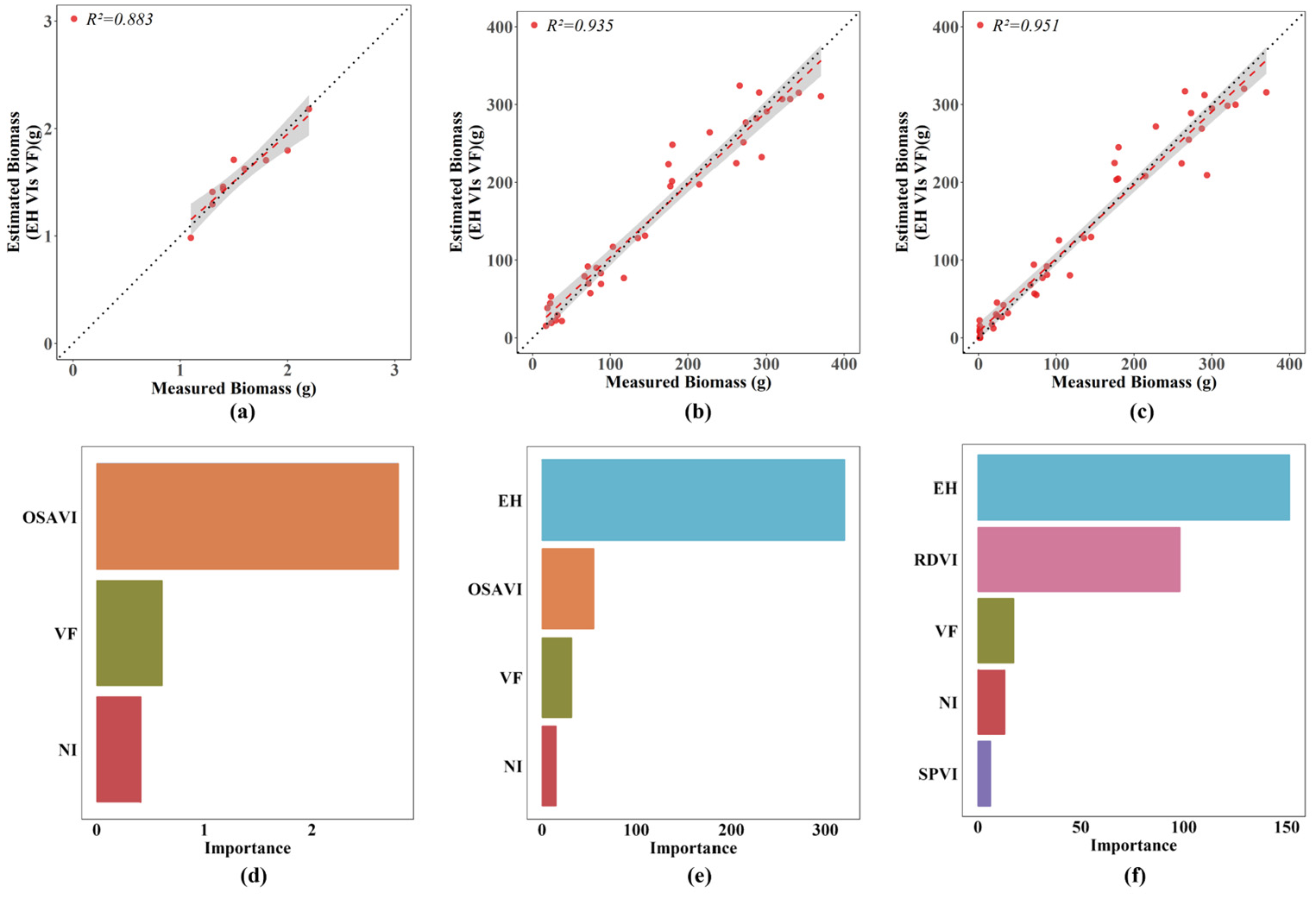
We normalized combined parameters prior to modeling. The LASSO method was applied to select the most relevant parameters. Selected parameters are used to build the PLSR model (Table 5). At the seedling stage (Figure 10a), the combination of OSAVI, NI and VF yields a strong fit between estimated dry biomass (EDB) and measured dry biomass (MDB) (R2 = 0.883). Variable importance in projection (VIP) analysis (Figure 10d) identifies OSAVI as the highest estimator. Notably, EH is not selected by LASSO for this stage, which is consistent with its lack of significant linear correlation with MDB, as observed earlier. At the non-seedling stage, the model combining EH, OSAVI, NI and VF further improves the estimation performance, achieving an R2 of 0.935 (Figure 10b). VIP analysis (Figure 10e) reveals that EH is the most influential estimator, followed by GNDVI. During the overall growth stage (Figure 10c), the model incorporating additional canopy VIs (NI and SPVI) alongside EH further boosts performance, yielding an R2 of 0.951. VIP analysis (Figure 10f) indicates that EH and RDVI are the primary estimators. Across all stages, PLSR models achieve R2 values above 0.8, confirming that integrating EH, VIs, and VF substantially improves biomass estimation.
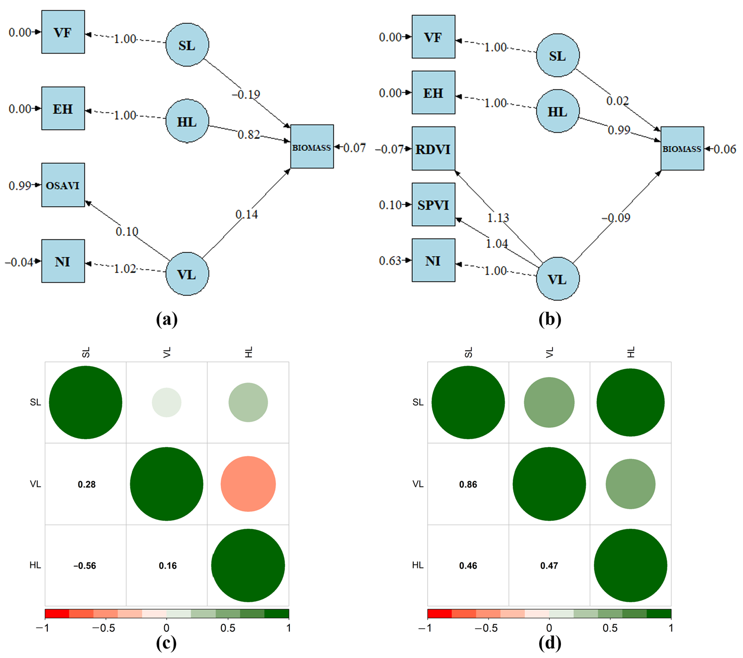
To gain deeper insights into how the combined parameters affect the MDB, we used structural equation modeling (SEM) with partial least squares path modeling (PLS-PM) to analyze the relationships for the overall growth stage and the non-seedling stage. In each case, the established MDB estimation model incorporated multiple variables, which represent distinct aspects of the canopy and growth structure. The variables were categorized into three latent variable groups: SL (related to structure, represented by VF—the vertical projection canopy cover fraction), VL (related to canopy status, represented by VIs), and HL (related to height, represented by EH). These latent variables were then used to explain their relationship with the latent variable BL, which represents the EDB. The model was designed for exploratory path analysis, and its performance was evaluated using PLS-guided standards, including the explained variance (R2) and bootstrapped confidence intervals of the path coefficients, and a descriptive global goodness-of-fit (GoF) index.
At the non-seedling stage (Figure 11a), the result reveals that HL exerts the strongest positive influence on BL (path coefficient of 0.82), confirming a major contribution of height. VL also shows a positive effect (coefficient of 0.14), while SL has a negative effect (coefficient of −0.19). The model accounts for a large proportion of the variation in biomass, with an R2 value of 0.924 for BL and an overall GoF of 0.660. The bootstrap results further show that only the effect of the HL on biomass is statistically supported, with an estimated coefficient of 0.815 and a 95% confidence interval ranging from 0.672 to 0.918. In contrast, the contributions of the VL and the SL are weak and not supported by the bootstrap test. The correlation matrix for these latent variables is shown in Figure 11c. Across the overall growth period (Figure 11b), HL shows the largest positive effect on BL (coefficient of 0.99), whereas the effects of VL and SL are minimal (coefficients of −0.09 and 0.02, respectively). Similarly, the model exhibits strong explanatory power, with the R-squared for BL reaching 0.937 and the goodness-of-fit value reaching 0.922. The bootstrap results indicate that the influence of HL on BL remains the only statistically supported effect, with a standardized coefficient of 0.979 and a 95% confidence interval ranging from 0.935 to 1.026. The correlation matrix for these latent variables is shown in Figure 11d.
Analysis of the outer weights reveals the relative importance of individual observed variables within their latent groups. At the non-seedling stage, NI (weight = 1.02) had a stronger influence on VL than OSAVI (weight = 0.1). Across the overall growth period, NI and SPVI in RDVI contributed to VL with 1.0, 1.04 and 1.13 weights, respectively, emphasizing the stronger influence of all nitrogen-related, health-related and chlorophyll-related latent variables. EH and VF are the only contributors to HL and SL, respectively, each with a weight of 1.00. The SEM analysis above provides a comprehensive framework, highlighting EH as the dominant driver of biomass accumulation, with VIs and VF acting as complementary factors, and elucidating their interactions.

5. Discussion

5.1. Analysis of Height Estimation Performance

The relationship between measured height (MH) and estimated height (EH) varied significantly across different stages, highlighting key considerations for UAV photogrammetry in height estimation. At the seedling stage, the poor correlation (R2 = 0.02) between MH and EH was attributed to the low crop height and sparse, discontinuous canopy structure, which left a large fraction of soil background exposed so that the 3D reconstruction was dominated by ground features, while the canopy height signal was comparable to photogrammetric uncertainties (e.g., image-matching noise and outliers/mixed ground–canopy points), thereby limiting the effective use of UAV photogrammetry [58] and leading to large relative errors in EH. In contrast, during the tillering and stem elongation stages, the MH–EH relationship improved substantially, with R2 reaching 0.864 at the stem elongation stage. These results indicate that UAV photogrammetry is highly effective once the crop reaches a sufficient height and canopy density [59].
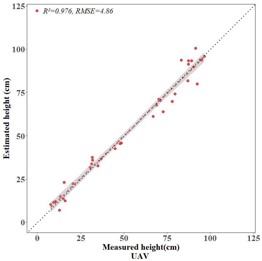
Using non-seedling stage data alone yielded a very strong linear fit between MH and EH, with an R2 of 0.976 and an RMSE of 4.86 cm, as can be seen in Figure 12. Section 4.2 indicates that the built model showed little to no linearity in the seedling stage. However, adding the seedling stage data left R2 essentially unchanged but raises RMSE from 4.86 cm to 11.65 cm.
Table 6 shows more details of the model at the non-seedling and overall stages. This is consistent with previous studies reporting high accuracy in UAV-based height estimation [60]. However, it is crucial to recognize that UAV-derived heights cannot fully replace ground measurement heights, especially when the crop is short and the canopy density is low.

5.2. Analysis of SPAD Estimation Performance Based on Vegetation Indices

The vegetation indices (VIs) combination for optimal SPAD (Soil and Plant Analyzer Development) value estimation varies at different stages (Table 7). The nuanced correlation observed at different stages between the VIs and SPAD value highlights the complexity of assessing relative chlorophyll content. The inclusion of OSAVI at both seedling and non-seedling stages improves SPAD estimation, likely because OSAVI accounts for background soil reflectance and canopy structure [61]. The observed correlations align with previous studies on other cereal crops, where at the seedling stage, sparse vegetation and greater soil background influence challenge the reliability of VIs [62].
Notably, soil background disturbance was strongest at the seedling stage because of the low fractional vegetation cover, leading to mixed soil–vegetation reflectance and potentially weakening conventional VI–SPAD linkages. However, soil-adjusted indices such as OSAVI were designed to suppress soil reflectance effects, which helped to explain why the seedling-stage model can still achieve a comparatively better performance than the non-seedling and overall stage settings. As the canopy developed and closed, the observed reflectance became increasingly influenced by canopy architecture (e.g., leaf area index, leaf-angle distribution) and shadowing/multiple scattering, and some VIs exhibited saturation; these factors could reduce the sensitivity of canopy-scale indices to leaf-level chlorophyll variability, contributing to weaker VI- SPAD correlations at later stages.

5.3. Analysis of Measured Dry Biomass Estimation

Dry biomass reflects the total nutrient content of rye and serves as a critical metric for evaluating its value as green manure in subsequent cash-crop rotations [62]. Table 8 lists all the regression formulas for modeling measured dry biomass (MDB), using single and combined parameters at different stages.
Our results reaffirmed a strong linear relationship between plant height and dry biomass. On-site measured height and UAV-estimated height both correlated closely with MDB, with only a slight advantage for the on-site measurements. The R2 of MH–MDB and EH–MDB differed by 2.15 % in the non-seedling stage and 2.11 % in the overall growth stage. Notably, EH data in the non-seedling stage proved largely unreliable, contributing to the greater discrepancy between MH–MDB and EH–MDB.
Previous studies have reported moderate success in UAV-based biomass estimation. Gustavo Togeirode Alckmin et al. conducted a field experiment at the Tasmanian Dairy Research Facility in Elliott to estimate rye biomass using both UAV-based multispectral imagery and proximal hyperspectral sensing. Following mission planning and radiometric correction of UAV imagery, spectral data were analyzed alongside reference biomass measurements. Biomass modeling was performed using Cubist regression trees. The study compared matching spectral measurements of observations acquired from a UAV-mounted multispectral camera (Parrot Sequoia) and handheld hyperspectral sensors. The highest biomass prediction accuracy from UAV data was achieved using the Sequoia 2018 dataset, with an R2 of 0.73 [63]. Additionally, Zhikai Cheng et al. conducted field experiments across two wheat-growing seasons and one maize-growing season. Their study proposed an effective method for estimating crop above-ground biomass (AGB) under film-mulched conditions, using UAV-based multispectral imagery from the DJI Phantom 4 Multispectral. The approach involved spectral index reconstruction using Lasso regression and a Bayesian ensemble model integrating machine learning algorithms, including PLSR with k-fold cross-validation. The method was validated across different years and crop types to assess the generalizability. The highest AGB prediction accuracy was achieved for film-mulched wheat, with an R2 of 0.84 [48]. In comparison, our models—combining biochemical–empirical vegetation index grouping with Lasso-based feature selection and PLSR with k-fold cross-validation—achieved a slightly higher R2 of 0.851 at the non-seedling stage, using the Phantom 4 Multispectral UAV platform.
Previous studies have demonstrated the value of combining multiple data sources for biomass estimation. Ang Chen et al. conducted their study in the temperate grasslands of Xilinhot City and Sonid Left Banner, Inner Mongolia, using a DJI Matrice 300 equipped with a Zenmuse L1 sensor to collect RGB imagery and LiDAR point clouds at a flight altitude of 350 m. While LiDAR features alone achieved limited performance (R2 = 0.404), the integration of RGB and hyperspectral features significantly improved estimation accuracy (R2 = 0.848). The highest R2 of 0.856 was achieved by combining RGB, hyperspectral, and LiDAR features [50]. Dunliang Wang et al. conducted winter wheat trials over two growing seasons at the experimental fields of Fengling Reservoir in Yizheng City, Jiangsu Province. UAV flights were carried out at an altitude of 25 m, using RGB-based color indices and DEM data to estimate wheat biomass. Using PLSR, their model achieved a maximum R2 of 0.90 [64]. Jibo Yue et al. conducted field experiments in the Changping District of Beijing, China, using UAV flights at approximately 50 m to monitor winter wheat. By combining UAV-derived DSM height with hyperspectral data and applying a MIMO-ANN model, they achieved a maximum R2 of 0.93 in estimating the above-ground biomass of vertically growing crops. [60]. For winter rye, all input parameters—including vegetation fraction, a suite of biochemistry-oriented vegetation indices, and photogrammetric canopy height—were extracted exclusively from the same set of multispectral UAV images. With no auxiliary hyperspectral or LiDAR data, the resulting model attained an R2 of 0.935 at the non-seedling stage and an R2 of 0.951 when all growth stages were considered. The improvement was largely attributable to the very low flight altitude (8–12 m), which delivered centimeter-scale ground resolution, together with a rigorous radiometric and geometric preprocessing workflow. These results demonstrate that, when high-quality multispectral data are coupled with biologically informed feature engineering, a lightweight UAV platform can be sufficient for precise trait estimation in rye, underscoring its suitability for scalable and cost-effective field phenotyping.

5.4. Latent Variable Analysis for MDB Estimation

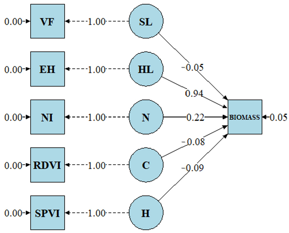
It is important to note that both height and spectral data differ in units from biomass, making biomass estimation essentially a model-fitting process. Notably, previous studies have not conducted attribution analysis to assess how individual parameters contribute to biomass estimation. This often results in high-performance models that are effectively uninterpretable, limiting both scientific insight and practical application. The PLS-PM SEM in Section 4.5 further revealed the effects of different parameters and their corresponding latent variables on biomass. Three latent variables were constructed: HL (height-related), SL (canopy structure), and VL (vegetation indices). Among these, HL showed the strongest impact on biomass, while SL and VL also contributed. The vegetation indices were functionally categorized (Table 2). To refine the analysis, VL was further divided into three functional categories: N (NI, linked to nitrogen accumulation), C (RDVI, representing relative chlorophyll content), and H (SPVI, indicating overall crop health). This functional decomposition of the spectral signal is a critical step, allowing us to move beyond a generic ‘greenness’ metric to probe specific physiological drivers. As shown in Figure 13, the SEM accounted for most of the variation in the biomass, with the R2 for biomass reaching 0.950. The results indicated that the HL exerted the strongest positive influence on biomass, with a path coefficient of 0.94. Among the decomposed vegetation index components, only the nitrogen-related category received additional statistical support, with a positive coefficient of 0.22, highlighting the close link between nitrogen status and biomass accumulation. By contrast, the effects associated with SL and the other VI categories are not statistically supported in the bootstrap test. By tracing the model’s estimation performance back to distinct, agronomically relevant traits, this analysis provides the granular, mechanistic insight that conventional modeling approaches lack, forming the primary advantage of our framework.
For completeness, we also report conventional global fit indices for this confirmatory SEM specification. The chi-square statistic is 5.630 with five degrees of freedom (p = 0.344). The goodness-of-fit index (GFI) is 0.965, the comparative fit index (CFI) is 0.999, and the Tucker–Lewis index (TLI) is 0.996. The root mean square error of approximation (RMSEA) is 0.052 and the standardized root mean square residual (SRMR) is 0.014. A global GoF index is not available when all constructs are modeled as single-indicator constructs.

5.5. Limitations and Future Work

This study has several limitations. UAV photogrammetry-based height estimation is less reliable in heterogeneous fields, especially during the seedling stage when canopy coverage is sparse. To improve reliability at the seedling stage, future work will focus on the fusion of LiDAR data with multispectral UAV imagery, which is expected to provide more robust three-dimensional structural information under sparse canopy conditions. SPAD (Soil and Plant Analyzer Development) estimation using the P4M UAV is also constrained by sensor hardware limitations and the sensitivity of vegetation index definitions. To address this, future studies will employ hyperspectral cameras to acquire richer spectral information across a wider range of wavelengths, enabling more accurate characterization of crop physiological status. Another potential limitation of this study is the limited amount of data. Although cross-validation was employed during modeling to enhance model reliability, the relatively small dataset may still restrict the generalization ability of the proposed models.
Future work should conduct larger-scale field trials and validate the model across multiple growing seasons to comprehensively address the data limitations and to improve the robustness and generalization capability of the proposed models. In particular, future work should extend beyond rye to include other crops, explicitly evaluating cross-crop transferability and investigating transfer learning strategies to enhance generalization. Upgrading to UAV platforms with reference panels or bidirectional reflectance capabilities may further enhance data validity. Moreover, the integration of advanced deep learning algorithms holds potential for further improving biomass estimation performance in larger-scale field trials in future works.

6. Conclusions

This study leveraged UAV photogrammetry using the P4M platform to successfully capture morphological and spectral information of a rye field, including the estimated canopy height (EH), vegetation indices (VIs), and vegetation fraction (VF). We adopted a preprocessing approach, applied machine learning algorithms for constructing masks, and then built statistical models of height, SPAD (Soil and Plant Analyzer Development), and dry biomass estimation. We obtained the measured height (MH), SPAD, and measured dry biomass (MDB) of each growth period from the field. Our results validated the linear relationship between the EH and MH, while reaffirming the significant correlation between the EH and MDB. In addition, our results validated the correlation between VIs and MDB. Ultimately, by integrating the EH with VIs and VF, we developed a robust multi-parameter biomass estimation model that demonstrates superior predictive performance compared to models using any single parameter. The key innovation of this work, however, lies in its shift from estimation to explanation. The application of PLS-PM structural equation modeling enables a detailed attribution analysis via latent variables, revealing the distinct and synergistic contributions of height, canopy structure, and spectral parameters to biomass accumulation.
Overall, this study established a high-efficiency biomass estimation framework based on low-altitude UAV remote sensing, demonstrating superior performance compared with the existing research reports. Although limitations remain, including the focus on a single experimental area, a single crop, and a single growing season, the conceptual framework proposed in this study provides a transferable reference for biomass modeling in other crop systems. Addressing these limitations and extending the framework to broader scenarios will constitute the main direction of future research.

Author Contributions

Conceptualization, W.L., M.K. and T.O.; methodology, W.L.; software, W.L., M.K. and T.O.; validation, W.L.; formal analysis, W.L., X.Z. and S.Y.; investigation, W.L.; resources, X.Z., M.K., T.O. and N.C.; data curation, W.L. and M.K.; writing—original draft preparation, W.L.; writing—review and editing, W.L., X.Z. and S.Y.; visualization, W.L. and X.Z.; supervision, X.Z., M.K. and T.O.; project administration, M.K.; funding acquisition, X.Z. and N.C. All authors have read and agreed to the published version of the manuscript.

Funding

This work was supported by National Key Research and Development Project of China (2025YFE0103300), Natural Science Foundation of China (42461144214; 42471349), Key Research and Development Project of Hubei Province (2024BCB101), Guangdong Basic and Applied Research Foundation (2024A1515030078), Shenzhen Science and Technology Program (JCYJ20240813114013017), Natural Science Foundation of Wuhan (2024040801020279), and Guided Project of Hubei Provincial Department of Education (B2023246).

Data Availability Statement

The data presented in this study are available upon request from the corresponding author.

Acknowledgments

We are particularly grateful to Masaki Yokoyama for his invaluable help with the RTK data measurement.

Conflicts of Interest

The authors declare no conflicts of interest.

Appendix A

Table A1. Candidate hyperparameter space used for the coarse-grid search.
ModelHyperparameterCandidate ValuesOptimal Value
RFtrees{50, 100, 150, 200}100
maximum depth{10, 15, 20, 25, 30}25
minimum samples per leaf{1, 3, 5, 7}5
SVMkernel{Linear, RBF}RBF
C{0.1, 0.5, 1.0, 2.0, 5.0, 10.0}1.0
γ{0.1, 0.5, 1.0, 2.0, 5.0, 10.0}2.0
ANN–GAhidden layers{(16, 8), (32, 16), (64, 32)}(32, 16)
population size{6, 8, 10, 12}8
parents per generation{2, 4, 6}4
generations{50,80,100,150}100
mutation rate{5%,10%,15%,20%}10%
KNNweights{Uniform, Distance}Uniform
distance metric{Euclidean, Manhattan}Euclidean

Appendix B

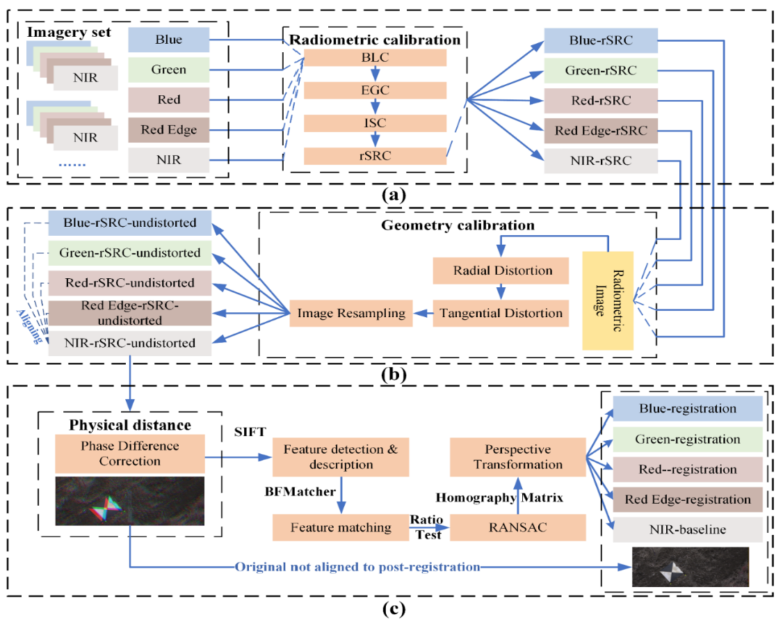
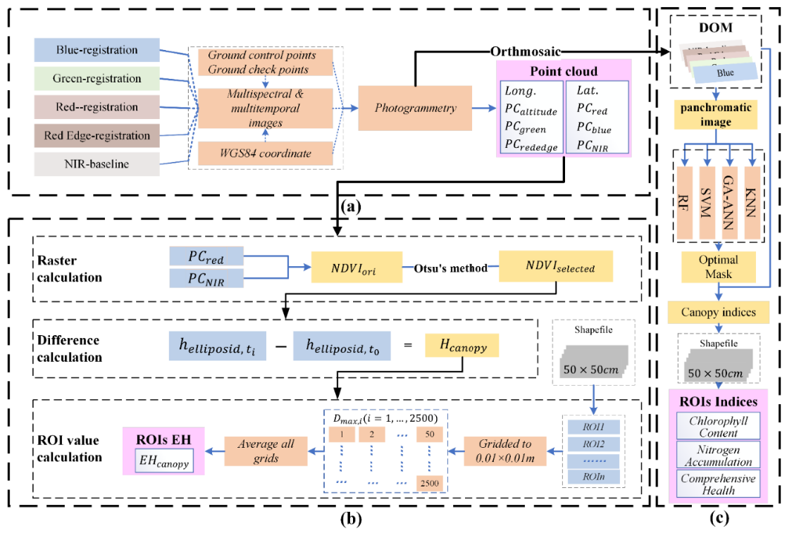
This appendix provides schematic overviews of the processing workflows corresponding to Section 3.1 and Section 3.3, aiming to further clarify the methodological framework. Figure A1 presents the complete image preprocessing procedure described in Section 3.1, including radiometric calibration, geometric distortion correction, and image registration. Figure A2 illustrates the canopy height model (CHM) construction and vegetation index generation process described in Section 3.3, including 3D reconstruction, NDVI-based canopy segmentation, height differencing, and ROI-based statistical analysis.
Figure A1. Overview of the key image preprocessing methods: (a) radiometric calibration workflow; (b) geometric distortion correction model; and (c) position offset correction and registration process.
Remotesensing 18 00665 g0a1
Figure A2. Overview of canopy crop height model (CHM) and canopy vegetation indices generation process. (a) Generation of 3D point cloud and digital orthomosaic map (DOM); (b) estimated height of canopy of region of interest derived from CHM; and (c) canopy vegetation indices of ROI calculated from DOM.
Remotesensing 18 00665 g0a2

References

  1. Li, X.; Zhao, L.; Zhang, T.; Zhang, Z.; Fu, S. Assessing the Impacts of Dry-Heat Extremes on Grassland Gross Primary Productivity across Mainland China Using Multi-Source Remote Sensing Data. Inf. Geogr. 2026, 2, 100038. [Google Scholar] [CrossRef]
  2. Dahal, K.; Talchabhadel, R.; Pradhan, P.; Parajuli, S.; Shrestha, D.; Chhetri, R.; Gautam, A.P.; Tamrakar, R.; Gurung, S.; Kumar, S. Nepal’s Carbon Stock and Biodiversity Are under Threat from Climate Exacerbated Forest Fires. Inf. Geogr. 2025, 1, 100003. [Google Scholar] [CrossRef]
  3. Bazzo, C.O.G.; Kamali, B.; Vianna, M.d.S.; Behrend, D.; Hueging, H.; Jahanbakhshi, F.; Schleip, I.; Mosebach, P.; Haub, A.; Behrendt, A.; et al. Grassland Ecosystem Assessments: Integrating UAV-Derived Features for Aboveground Biomass Estimation. Inf. Process. Agric. 2026, in press. [Google Scholar] [CrossRef]
  4. Breunig, F.M.; Galvão, L.S.; Dalagnol, R.; Santi, A.L.; Della Flora, D.P.; Chen, S. Assessing the Effect of Spatial Resolution on the Delineation of Management Zones for Smallholder Farming in Southern Brazil. Remote Sens. Appl. Soc. Environ. 2020, 19, 100325. [Google Scholar] [CrossRef]
  5. Baraibar, B.; Mortensen, D.; Hunter, M.C.; Barbercheck, M.; Kaye, J.; Finney, D.; Curran, W.; Bunchek, J.; White, C. Growing Degree Days and Cover Crop Type Explain Weed Biomass in Winter Cover Crops. Agron. Sustain. Dev. 2018, 38, 65. [Google Scholar] [CrossRef]
  6. Mareya, H.T.; Tagwireyi, P.; Ndaimani, H.; Gara, T.W.; Gwenzi, D. Estimating Tree Crown Area and Aboveground Biomass in Miombo Woodlands from High-Resolution RGB-Only Imagery. IEEE J. Sel. Top. Appl. Earth Obs. Remote Sens. 2018, 11, 868–875. [Google Scholar] [CrossRef]
  7. Estornell, J.; Martí, J.; Hadas, E.; López-Cortés, I.; Velázquez-Martí, B.; Fernández-Sarría, A. Biomass Estimation of Abandoned Orange Trees Using UAV-SFM 3D Points. Int. J. Appl. Earth Obs. Geoinf. 2024, 130, 103931. [Google Scholar] [CrossRef]
  8. Huang, Y.; Qiu, B.; Yang, P.; Wu, W.; Zhu, W.; Yuan, W.; Chen, J.; Chen, X.; Zhu, X.; Xu, S.; et al. A Hierarchy Framework for Automatic Mapping Complex Rice Cropping Patterns: National-Scale Annual Datasets of ChinaCP-Rice10m during 2019–2024. Inf. Geogr. 2026, 2, 100033. [Google Scholar] [CrossRef]
  9. Adeluyi, O.; Harris, A.; Foster, T.; Clay, G.D. Exploiting Centimetre Resolution of Drone-Mounted Sensors for Estimating Mid-Late Season above Ground Biomass in Rice. Eur. J. Agron. 2022, 132, 126411. [Google Scholar] [CrossRef]
  10. Teshome, F.T.; Bayabil, H.K.; Hoogenboom, G.; Schaffer, B.; Singh, A.; Ampatzidis, Y. Unmanned Aerial Vehicle (UAV) Imaging and Machine Learning Applications for Plant Phenotyping. Comput. Electron. Agric. 2023, 212, 108064. [Google Scholar] [CrossRef]
  11. Romero, A.G.; Lopes, M.S. Heading and Maturity Date Prediction Using Vegetation Indices: A Case Study Using Bread Wheat, Barley and Oat Crops. Eur. J. Agron. 2024, 160, 127330. [Google Scholar] [CrossRef]
  12. Liu, Y.; Liu, S.; Li, J.; Guo, X.; Wang, S.; Lu, J. Estimating Biomass of Winter Oilseed Rape Using Vegetation Indices and Texture Metrics Derived from UAV Multispectral Images. Comput. Electron. Agric. 2019, 166, 105026. [Google Scholar] [CrossRef]
  13. Marshall, M.; Thenkabail, P. Advantage of Hyperspectral EO-1 Hyperion over Multispectral IKONOS, GeoEye-1, WorldView-2, Landsat ETM+, and MODIS Vegetation Indices in Crop Biomass Estimation. ISPRS J. Photogramm. Remote Sens. 2015, 108, 205–218. [Google Scholar] [CrossRef]
  14. Fei, S.; Xiao, S.; Li, Q.; Shu, M.; Zhai, W.; Xiao, Y.; Chen, Z.; Yu, H.; Ma, Y. Enhancing Leaf Area Index and Biomass Estimation in Maize with Feature Augmentation from Unmanned Aerial Vehicle-Based Nadir and Cross-Circling Oblique Photography. Comput. Electron. Agric. 2023, 215, 108462. [Google Scholar] [CrossRef]
  15. Shen, S.; Li, W.; Zou, J.; Harrison, M.T.; Liu, S.; Eyshi Rezaei, E.; Liu, K.; Kamali, B.; Wang, Z.; Zhang, D.; et al. Fusing UAV Multiple Data and Phenology to Predict Crop Biomass. Inf. Process. Agric. 2025, in press. [Google Scholar] [CrossRef]
  16. Zhang, S.-H.; He, L.; Duan, J.-Z.; Zang, S.-L.; Yang, T.-C.; Schulthess, U.R.S.; Guo, T.-C.; Wang, C.-Y.; Feng, W. Aboveground Wheat Biomass Estimation from a Low-Altitude UAV Platform Based on Multimodal Remote Sensing Data Fusion with the Introduction of Terrain Factors. Precis. Agric. 2024, 25, 119–145. [Google Scholar] [CrossRef]
  17. Feng, Z.; Yang, Z.; Suo, L.; Wu, K.; Ma, Z.; Zhang, H.; Duan, J.; Feng, W. Enhancing Maize Above-Ground Biomass Estimation through Multispectral, Digital and LiDAR Fusion on UAV Platforms. Agric. Water Manag. 2025, 315, 109551. [Google Scholar] [CrossRef]
  18. Bendig, J.; Yu, K.; Aasen, H.; Bolten, A.; Bennertz, S.; Broscheit, J.; Gnyp, M.L.; Bareth, G. Combining UAV-Based Plant Height from Crop Surface Models, Visible, and near Infrared Vegetation Indices for Biomass Monitoring in Barley. Int. J. Appl. Earth Obs. Geoinf. 2015, 39, 79–87. [Google Scholar] [CrossRef]
  19. Biswal, S.; Pathak, N.; Chatterjee, C.; Mailapalli, D.R. Estimation of Aboveground Biomass from Spectral and Textural Characteristics of Paddy Crop Using UAV-Multispectral Images and Machine Learning Techniques. Geocarto Int. 2024, 39, 2364725. [Google Scholar] [CrossRef]
  20. Li, J.; Li, J.; Zhao, D.; Cao, Q.; Yu, F.; Cao, Y.; Feng, S.; Xu, T. High-Throughput Method for Improving Rice AGB Estimation Based on UAV Multi-Source Remote Sensing Image Feature Fusion and Ensemble Learning. Front. Plant Sci. 2025, 16, 1576212. [Google Scholar] [CrossRef]
  21. Shafiee, S.; Mroz, T.; Burud, I.; Lillemo, M. Evaluation of UAV Multispectral Cameras for Yield and Biomass Prediction in Wheat under Different Sun Elevation Angles and Phenological Stages. Comput. Electron. Agric. 2023, 210, 107874. [Google Scholar] [CrossRef]
  22. Deng, L.; Hao, X.; Mao, Z.; Yan, Y.; Sun, J.; Zhang, A. A Subband Radiometric Calibration Method for UAV-Based Multispectral Remote Sensing. IEEE J. Sel. Top. Appl. Earth Obs. Remote Sens. 2018, 11, 2869–2880. [Google Scholar] [CrossRef]
  23. Mzid, N.; Pignatti, S.; Huang, W.; Casa, R. An Analysis of Bare Soil Occurrence in Arable Croplands for Remote Sensing Topsoil Applications. Remote Sens. 2021, 13, 474. [Google Scholar] [CrossRef]
  24. Chen, Q.; Vaudour, E.; Richer-de-Forges, A.C.; Arrouays, D. Spectral Indices in Remote Sensing of Soil: Definition, Popularity, and Issues. A Critical Overview. Remote Sens. Environ. 2025, 329, 114918. [Google Scholar] [CrossRef]
  25. Demattê, J.A.M.; Safanelli, J.L.; Poppiel, R.R.; Rizzo, R.; Silvero, N.E.Q.; Mendes, W.d.S.; Bonfatti, B.R.; Dotto, A.C.; Salazar, D.F.U.; Mello, F.A.d.O.; et al. Bare Earth’s Surface Spectra as a Proxy for Soil Resource Monitoring. Sci. Rep. 2020, 10, 4461. [Google Scholar] [CrossRef]
  26. Nguyen, T.L.V.; Apopei, B.; Alameh, K. Effective Plant Discrimination Based on the Combination of Local Binary Pattern Operators and Multiclass Support Vector Machine Methods. Inf. Process. Agric. 2019, 6, 116–131. [Google Scholar] [CrossRef]
  27. Xue, B.; Yu, C.; Wang, Y.; Song, M.; Li, S.; Wang, L.; Chen, H.-M.; Chang, C.-I. A Subpixel Target Detection Approach to Hyperspectral Image Classification. IEEE Trans. Geosci. Remote Sens. 2017, 55, 5093–5114. [Google Scholar] [CrossRef]
  28. Meng, Y.; Hu, Z.; Chen, X.; Yao, J. Subtracted Histogram: Utilizing Mutual Relation Between Features for Thresholding. IEEE Trans. Geosci. Remote Sens. 2018, 56, 7415–7435. [Google Scholar] [CrossRef]
  29. Breiman, L. Random Forests. Mach. Learn. 2001, 45, 5–32. [Google Scholar] [CrossRef]
  30. Cortes, C.; Vapnik, V. Support-Vector Networks. Mach. Learn. 1995, 20, 273–297. [Google Scholar] [CrossRef]
  31. Kitano, H. Neurogenetic Learning: An Integrated Method of Designing and Training Neural Networks Using Genetic Algorithms. Phys. D Nonlinear Phenom. 1994, 75, 225–238. [Google Scholar] [CrossRef]
  32. Cover, T.; Hart, P. Nearest Neighbor Pattern Classification. IEEE Trans. Inf. Theory 1967, 13, 21–27. [Google Scholar] [CrossRef]
  33. Zhu, Y.; Yao, X.; Tian, Y.; Liu, X.; Cao, W. Analysis of Common Canopy Vegetation Indices for Indicating Leaf Nitrogen Accumulations in Wheat and Rice. Int. J. Appl. Earth Obs. Geoinf. 2008, 10, 1–10. [Google Scholar] [CrossRef]
  34. Tian, Y.C.; Yao, X.; Yang, J.; Cao, W.X.; Hannaway, D.B.; Zhu, Y. Assessing Newly Developed and Published Vegetation Indices for Estimating Rice Leaf Nitrogen Concentration with Ground- and Space-Based Hyperspectral Reflectance. Field Crops Res. 2011, 120, 299–310. [Google Scholar] [CrossRef]
  35. Wang, W.; Yao, X.; Yao, X.; Tian, Y.; Liu, X.; Ni, J.; Cao, W.; Zhu, Y. Estimating Leaf Nitrogen Concentration with Three-Band Vegetation Indices in Rice and Wheat. Field Crops Res. 2012, 129, 90–98. [Google Scholar] [CrossRef]
  36. Khan, M.S.; Yadav, P.; Semwal, M.; Prasad, N.; Verma, R.K.; Kumar, D. Predicting Canopy Chlorophyll Concentration in Citronella Crop Using Machine Learning Algorithms and Spectral Vegetation Indices Derived from UAV Multispectral Imagery. Ind. Crops Prod. 2024, 219, 119147. [Google Scholar] [CrossRef]
  37. Zhang, B.; Gu, L.; Dai, M.; Bao, X.; Sun, Q.; Qu, X.; Zhang, M.; Liu, X.; Fan, C.; Gu, X.; et al. Estimation of Grain Filling Rate and Thousand-Grain Weight of Winter Wheat (Triticum aestivum L.) Using UAV-Based Multispectral Images. Eur. J. Agron. 2024, 159, 127258. [Google Scholar] [CrossRef]
  38. Bannari, A.; Khurshid, K.S.; Staenz, K.; Schwarz, J.W. A Comparison of Hyperspectral Chlorophyll Indices for Wheat Crop Chlorophyll Content Estimation Using Laboratory Reflectance Measurements. IEEE Trans. Geosci. Remote Sens. 2007, 45, 3063–3074. [Google Scholar] [CrossRef]
  39. Rondeaux, G.; Steven, M.; Baret, F. Optimization of Soil-Adjusted Vegetation Indices. Remote Sens. Environ. 1996, 55, 95–107. [Google Scholar] [CrossRef]
  40. Sonobe, R.; Sano, T.; Horie, H. Using Spectral Reflectance to Estimate Leaf Chlorophyll Content of Tea with Shading Treatments. Biosyst. Eng. 2018, 175, 168–182. [Google Scholar] [CrossRef]
  41. Gitelson, A.A.; Kaufman, Y.J.; Merzlyak, M.N. Use of a Green Channel in Remote Sensing of Global Vegetation from EOS-MODIS. Remote Sens. Environ. 1996, 58, 289–298. [Google Scholar] [CrossRef]
  42. Carlson, T.N.; Ripley, D.A. On the Relation between NDVI, Fractional Vegetation Cover, and Leaf Area Index. Remote Sens. Environ. 1997, 62, 241–252. [Google Scholar] [CrossRef]
  43. Roujean, J.-L.; Breon, F.-M. Estimating PAR Absorbed by Vegetation from Bidirectional Reflectance Measurements. Remote Sens. Environ. 1995, 51, 375–384. [Google Scholar] [CrossRef]
  44. Broge, N.H.; Leblanc, E. Comparing Prediction Power and Stability of Broadband and Hyperspectral Vegetation Indices for Estimation of Green Leaf Area Index and Canopy Chlorophyll Density. Remote Sens. Environ. 2001, 76, 156–172. [Google Scholar] [CrossRef]
  45. Shibayama, M.; Akiyama, T. Seasonal Visible, near-Infrared and Mid-Infrared Spectra of Rice Canopies in Relation to LAI and above-Ground Dry Phytomass. Remote Sens. Environ. 1989, 27, 119–127. [Google Scholar] [CrossRef]
  46. Junttila, V.; Kauranne, T.; Finley, A.O.; Bradford, J.B. Linear Models for Airborne-Laser-Scanning-Based Operational Forest Inventory with Small Field Sample Size and Highly Correlated LiDAR Data. IEEE Trans. Geosci. Remote Sens. 2015, 53, 5600–5612. [Google Scholar] [CrossRef]
  47. Sun, G.; Zhang, Y.; Chen, H.; Wang, L.; Li, M.; Sun, X.; Fei, S.; Xiao, S.; Yan, L.; Li, Y.; et al. Improving Soybean Yield Prediction by Integrating UAV Nadir and Cross-Circling Oblique Imaging. Eur. J. Agron. 2024, 155, 127134. [Google Scholar] [CrossRef]
  48. Cheng, Z.; Gu, X.; Zhou, Z.; Yin, R.; Zheng, X.; Li, W.; Cai, W.; Chang, T.; Du, Y. Crop Aboveground Biomass Monitoring Model Based on UAV Spectral Index Reconstruction and Bayesian Model Averaging: A Case Study of Film-Mulched Wheat and Maize. Comput. Electron. Agric. 2024, 224, 109190. [Google Scholar] [CrossRef]
  49. Shafiee, S.; Lied, L.M.; Burud, I.; Dieseth, J.A.; Alsheikh, M.; Lillemo, M. Sequential Forward Selection and Support Vector Regression in Comparison to LASSO Regression for Spring Wheat Yield Prediction Based on UAV Imagery. Comput. Electron. Agric. 2021, 183, 106036. [Google Scholar] [CrossRef]
  50. Chen, A.; Xu, C.; Zhang, M.; Guo, J.; Xing, X.; Yang, D.; Xu, B.; Yang, X. Cross-Scale Mapping of above-Ground Biomass and Shrub Dominance by Integrating UAV and Satellite Data in Temperate Grassland. Remote Sens. Environ. 2024, 304, 114024. [Google Scholar] [CrossRef]
  51. Yang, D.; Morrison, B.D.; Hanston, W.; McMahon, A.; Baskaran, L.; Hayes, D.J.; Miller, C.E.; Serbin, S.P. Integrating Very-High-Resolution UAS Data and Airborne Imaging Spectroscopy to Map the Fractional Composition of Arctic Plant Functional Types in Western Alaska. Remote Sens. Environ. 2023, 286, 113430. [Google Scholar] [CrossRef]
  52. Reinartz, W.; Haenlein, M.; Henseler, J. An Empirical Comparison of the Efficacy of Covariance-Based and Variance-Based SEM. Int. J. Res. Mark. 2009, 26, 332–344. [Google Scholar] [CrossRef]
  53. Kante, M.; Oboko, R.; Chepken, C. An ICT Model for Increased Adoption of Farm Input Information in Developing Countries: A Case in Sikasso, Mali. Inf. Process. Agric. 2019, 6, 26–46. [Google Scholar] [CrossRef]
  54. Tenenhaus, M.; Vinzi, V.E.; Chatelin, Y.-M.; Lauro, C. PLS Path Modeling. Comput. Stat. Data Anal. 2005, 48, 159–205. [Google Scholar] [CrossRef]
  55. Qiao, L.; Tang, W.; Gao, D.; Zhao, R.; An, L.; Li, M.; Sun, H.; Song, D. UAV-Based Chlorophyll Content Estimation by Evaluating Vegetation Index Responses under Different Crop Coverages. Comput. Electron. Agric. 2022, 196, 106775. [Google Scholar] [CrossRef]
  56. Yuan, Z.; Cao, Q.; Zhang, K.; Ata-Ul-Karim, S.T.; Tian, Y.; Zhu, Y.; Cao, W.; Liu, X. Optimal Leaf Positions for SPAD Meter Measurement in Rice. Front. Plant Sci. 2016, 7, 719. [Google Scholar] [CrossRef]
  57. Xiong, D.; Chen, J.; Yu, T.; Gao, W.; Ling, X.; Li, Y.; Peng, S.; Huang, J. SPAD-Based Leaf Nitrogen Estimation Is Impacted by Environmental Factors and Crop Leaf Characteristics. Sci. Rep. 2015, 5, 13389. [Google Scholar] [CrossRef]
  58. Xie, T.; Li, J.; Yang, C.; Jiang, Z.; Chen, Y.; Guo, L.; Zhang, J. Crop Height Estimation Based on UAV Images: Methods, Errors, and Strategies. Comput. Electron. Agric. 2021, 185, 106155. [Google Scholar] [CrossRef]
  59. Valluvan, A.B.; Raj, R.; Pingale, R.; Jagarlapudi, A. Canopy Height Estimation Using Drone-Based RGB Images. Smart Agric. Technol. 2023, 4, 100145. [Google Scholar] [CrossRef]
  60. Yue, J.; Yang, H.; Yang, G.; Fu, Y.; Wang, H.; Zhou, C. Estimating Vertically Growing Crop Above-Ground Biomass Based on UAV Remote Sensing. Comput. Electron. Agric. 2023, 205, 107627. [Google Scholar] [CrossRef]
  61. Wang, R.; Tuerxun, N.; Zheng, J. Improved Estimation of SPAD Values in Walnut Leaves by Combining Spectral, Texture, and Structural Information from UAV-Based Multispectral Image. Sci. Hortic. 2024, 328, 112940. [Google Scholar] [CrossRef]
  62. Breunig, F.M.; Galvão, L.S.; Dalagnol, R.; Dauve, C.E.; Parraga, A.; Santi, A.L.; Della Flora, D.P.; Chen, S. Delineation of Management Zones in Agricultural Fields Using Cover–Crop Biomass Estimates from PlanetScope Data. Int. J. Appl. Earth Obs. Geoinf. 2020, 85, 102004. [Google Scholar] [CrossRef]
  63. Togeirode Alckmin, G.; Lucieer, A.; Rawnsley, R.; Kooistra, L. Perennial Ryegrass Biomass Retrieval through Multispectral UAV Data. Comput. Electron. Agric. 2022, 193, 106574. [Google Scholar] [CrossRef]
  64. Wang, D.; Li, R.; Zhu, B.; Liu, T.; Sun, C.; Guo, W. Estimation of Wheat Plant Height and Biomass by Combining UAV Imagery and Elevation Data. Agriculture 2022, 13, 9. [Google Scholar] [CrossRef]
Figure 1. Location and experimental plot of the study area in Ibaraki Prefecture, Japan.
Remotesensing 18 00665 g001
Figure 2. Growth stages and sampling patterns of biomass in rye. (a) Schematic diagram of rye growth stages sampled in this study, and (b) sampling pattern used for biomass collection in experiment field.
Remotesensing 18 00665 g002
Figure 3. Visualization of the 3D dense point clouds generated for each growth stage: (a) 30 November 2020 (seedling), (b) 24 March 2021 (tillering), (c) 31 March 2021 (tillering), (d) 11 April 2021 (elongation), and (e) 21 April 2021 (heading), alongside (f) the reference point cloud from the fallow period prior to germination. The corresponding digitally mapped 50 × 50 cm sampling ROIs are also illustrated.
Remotesensing 18 00665 g003
Figure 4. Overview of the statistical analysis workflow used in this study.
Remotesensing 18 00665 g004
Figure 5. Orthomosaic classification maps of crop vegetation at different growth stages, generated using four machine learning classifiers: (a) ANN-GA, (b) KNN, (c) RF, and (d) SVM. In each map, white regions represent vegetation, while black regions denote non-vegetation areas.
Remotesensing 18 00665 g005
Figure 6. An OLS linear regression between MH and EH. (a) Linear relationship between MH and EH for each individual acquisition date: N1130 = 11 November 2020; N0324 = 24 March 2021; N0331 = 31 March 2021; N0411 = 11 April 2021; and N0421 = 21 April 2021. (b) Linear regression between MH and EH, using all combined data to represent an overall growth stage.
Remotesensing 18 00665 g006
Figure 7. Correlation matrices of SPAD and VIs at the (a) seedling stage, (b) non-seedling growth stage, and (c) overall growth stage (* p < 0.05, ** p < 0.01, and *** p < 0.001); MLR model between SPAD and VIs at the (d) seedling stage, (e) non-seedling stage, and (f) overall growth stage.
Remotesensing 18 00665 g007
Figure 8. Linear regression between MH and MDB at the (a) seedling stage, (b) non-seedling stage and (c) overall growth stage. Linear regression between EH and MDB at the (d) seedling stage, (e) non-seedling stage and (f) overall growth stage.
Remotesensing 18 00665 g008
Figure 9. Linear regression between estimated biomass and measured biomass at the (a) seedling stage, (b) non-seedling stage, and (c) overall growth stage, with the corresponding VIP plots shown in (df), respectively.
Remotesensing 18 00665 g009
Figure 10. The relationship between measured biomass and estimated biomass at the (a) seedling stage, (b) non-seedling stage, and (c) overall growth stage, with the corresponding VIP plots shown in (df), respectively.
Remotesensing 18 00665 g010
Figure 11. SEM results for EDB at the (a) non-seedling stage, and (b) overall growth stage. Correlation matrices of latent variables SL, HL, and VL are shown for the (c) non-seedling stage and (d) overall growth stage.
Remotesensing 18 00665 g011
Figure 12. Relationship between MH and EH data at the non-seedling stage.
Remotesensing 18 00665 g012
Figure 13. SEM results of biomass in full growth period after dividing VL into N, C and H.
Remotesensing 18 00665 g013
Table 1. Flight mission details and corresponding ground sampling information; GSD = ground sampling distance.
Flight DateSample DateStageFlight Height (m)Azimuth/Altitude (°)Obtained Information
Images
Collected
Number of BandsComposite
Images
GSD (mm/pix)
9 November 2020-fallow8151.54/32.025825972.38
30 November 20201 December 2020seedling8163.57/30.5472051202.39
24 March 202024 March 2020tillering12147.82/50.935765963.3
31 March 202031 March 2020tillering12262.9/13.7560051003.3
11 April 202011 April 2020elongation12189.40/62.045765963.3
21 April 202122 April 2021heading12270.87/19.495945993.28
Table 2. The equation of spectral vegetation indices for estimating canopy parameters and its modified definition.
ItemsVIEquationModified Definition Based on FC6360
Canopy
Chlorophyll
Index
GNDVI R 800 R 550 R 800   + R 550   NIR Green NIR Green
OSAVI 1.16   ×   ( R 800 R 670 ) R 800 + R 670   + 0.16 1.16   ×   NIR Red NIR + Red + 0.16
SPVI 1.48   ×   ( R 800 R 670 ) 1.2   ×   R 530 R 670 1.48   ×   ( NIR Red )   1.2   ×   Green Red
Canopy Health IndexRVI R 800 R 670 NIR Red
RDVI R 800 R 670 R 800 + R 670 NIR Red NIR + Red
NDVI R 800 R 670   R 800 + R 670   NIR RED NIR + RED
Canopy
Nitrogen Index
NI R 710 R 710 + R 470   RedEdge RedEdge + Blue
Table 3. Classification performance metrics of different machine learning algorithms on different dates.
StageMethodAccuracyPrecisionRecallF1 ScoreAUC
SeedlingANN-GA0.6520.6840.6670.6480.667
KNN0.9230.9180.8900.9040.975
RF0.9590.9670.9420.9540.995
SVM0.8810.9070.8230.8630.923
Tiller 1ANN-GA0.9490.9480.9500.9490.950
KNN1.0001.0001.0001.0001.000
RF1.0001.0001.0001.0001.000
SVM1.0001.0001.0001.0001.000
Tiller 2ANN-GA0.9200.4610.4580.4590.911
KNN0.9960.9940.9970.9951.000
RF1.0001.0001.0001.0001.000
SVM0.9981.0000.9940.9971.000
ElongationANN-GA0.6030.5810.5810.5810.581
KNN0.9850.9720.9890.9810.986
RF0.9970.9931.0000.9961.000
SVM0.9890.9760.9960.9860.999
HeadingANN-GA0.6350.6330.6090.6030.609
KNN0.9910.9870.9930.9900.997
RF1.0001.0001.0001.0001.000
SVM0.9930.9910.9930.9920.999
Table 4. Vegetation indices selected by the least absolute shrinkage and selection operator (LASSO) method for dry biomass estimation based on partial least squares regression (PLSR) at different stages.
StageVariables/Parameters
NDVIRDVIGNDVIOSAVISPVINI
Seedling1.428002.58100
Non-seedling623.0130830.172−1091.2670−456.024
All stages1592.4670720.434−763.558−1.171−503.793
Table 5. Multi-parameter feature sets selected by LASSO method for dry biomass estimation based on PLSR at different stages.
StageVariables/Parameters
EHNDVIRDVIGNDVIOSAVISPVINIVF
Seedling00002.0050−2.3815.158
Non-seedling273.920000−120.4290278.807−418.332
All stages321.1450−3.79800−0.255324.468−41.027
Table 6. Regression formulas for EH at different growth stages.
Estimated VariableStageRegression Formula
EHNon-seedling 0.871   ×   MH 2.333
All 0.893   ×   MH 4.273
Table 7. Regression formulas for SPAD at different growth stages.
Estimated VariableStageRegression Formula
SPADNon-seedling 21.421   ×   NDVI 5.251   ×   GNDVI + 27.829   ×   OSAVI + 42.186
Seedling 5.462   ×   OSAVI 0.027   ×   SPVI + 41.880
All 39.379   ×   NDVI 2.444   ×   GNDVI + 20.496   ×   OSAVI + 0.026   ×   SPVI + 61.104
Table 8. Regression formulas for MDB at different growth stages (*** p < 0.01; ** p < 0.05; * p < 0.1).
Estimated VariableUsed
Variable
StageRegression Formula
MDBEHSeedling 0.109   ×   EH + 1.230
Non-seedling 3.342   ×   EH   * * * 15.381
All 3.295   ×   EH   * * * 11.920
VIsSeedling 1.428   ×   NDVI + 2.581   ×   OSAVI   * + 0.127
Non-seedling 623.013   ×   NDVI   * + 830.172   ×   GNDVI   * * * 1091.267   ×   OSAVI   * * * 456.024   ×   NI   * + 411.109
All 1592.467   ×   NDVI   * * *   + 720.434   ×   GNDVI   * * * 763.558   ×   OSAVI   * * * 1.171   ×   SPVI   *     503.793   ×   NI   *     559.351
Combined ParametersSeedling 2.005   ×   OSAVI   * * * 2.381   ×   NI + 5.158   ×   VF   * * * + 1.808
Non-seedling 273.920   ×   EH   * * * 120.429   ×   OSAVI   *   +   278.807   ×   NI   * * 418.332   ×   VF   * *   +   122.712
All 321.145   ×   EH   * * * 3.798   ×   RDVI   ×   0.255   ×   SPVI + 324.468   ×   NI   * * 41.027   ×   VF 170.918
Disclaimer/Publisher’s Note: The statements, opinions and data contained in all publications are solely those of the individual author(s) and contributor(s) and not of MDPI and/or the editor(s). MDPI and/or the editor(s) disclaim responsibility for any injury to people or property resulting from any ideas, methods, instructions or products referred to in the content.