


Highlights
What are the main findings?
- A quality assessment method was proposed to assess the reliability of lidar raw data from the China Aerosol Raman Lidar Network (CARLNET), currently comprising 49 multiwavelength polarization Raman lidars used for meteorological and atmospheric-environment monitoring.
- The proposed quality assessment method can effectively distinguish lidar raw data quality under different scenarios. The assessment results can reveal certain lidar hardware issues and reflect the overall data quality situation of CARLNET.
What are the implications of the main findings?
- The lidar raw data is scored and labeled by the proposed quality assessment method, which provides support for lidar network data quality monitoring, operational applications, and scientific research.
- The assessment results can reflect potential issues of lidar systems, thereby providing guidance for equipment maintenance.
Abstract
The China Aerosol Raman Lidar Network (CARLNET), developed by the China Meteorological Administration, currently comprises 49 multiwavelength polarization Raman lidars used for meteorological and atmospheric-environment monitoring. Timely and automatic quality assessment of the lidar raw signal is vital for a large atmospheric lidar network. This study proposes a quality assessment method of lidar raw data for the CARLNET. By scoring three factors, signal saturation at near-range, Rayleigh fit and effective detection range, and weighting each influence factor according to its importance, each lidar raw data is tagged by a composite score. These scores reflect the quality of lidar raw data, as well as potential issues of lidar systems. Three lidars under three typical weather scenarios are used to analyze the impact of observation scenarios on lidar raw data, and the results show that the proposed method can effectively distinguish the lidar raw data quality under different scenarios. By analyzing the scores of lidar raw data, two potential hardware issues (optical-axis misalignment and signal-receiving issues) are identified, which provide guidance for equipment maintenance. In addition, we applied the method to one-year CARLNET measurement data. Temporally, five representative sites were selected for analysis of their annual data, revealing the seasonal and overall scores of the raw data. Spatially, the signals at the 355 nm, 532 nm, and 1064 nm channels of 49 nationwide distributed lidars were evaluated and categorized into six groups based on their scores, which provides support for lidar network data quality monitoring, operational applications, and scientific research.
1. Introduction
The scattering and absorption properties of aerosols directly impact the radiation balance [1,2,3] And these tiny particles play a crucial role in weather phenomena such as fog, haze and rain. Meanwhile, the large-scale transport of aerosols affects ecosystems [4,5,6]. Precise and reliable meteorological elements (such as aerosols, water vapor, etc.) are of vital importance for atmospheric and environmental scientific research and operational applications, which are always the goal in the fields of meteorological research and environmental monitoring [7,8,9,10,11]. Lidar has the advantages of high detection accuracy, long detection distance and continuous observation, which can accurately obtain the vertical distribution of atmospheric parameters [12,13,14,15,16]. It is an important observation method in the fields of climate and meteorology.
As lidar technology and emerging intelligent methodologies develop and scientific research expands, the demand for meteorological data on a large scale is increasing [17,18,19,20,21], and single lidar observations can no longer satisfy this demand. At present, lidar is developing in the direction of network observation. Ground-based lidar networks offer significant advantages when it comes to obtaining vertical profiles of aerosol optical properties on regional and even global scales. NASA developed the Micro Pulse Lidar Network (MPLNET) to monitor global clouds and aerosols [22,23,24,25]. The European Aerosol Research Lidar Network (EARLINET) was established to establish a continental-scale dataset on aerosol distributions that is comprehensive, quantitative, and of high statistical significance [26,27,28,29]. Referring to the experience gained from the long-term operation of the EARLINT, TROPOS developed and progressively refined the portable Polly lidar system, which led to the creation of PollyNET, a multiwavelength polarized Raman lidar network for remote observation of aerosols and clouds [30,31,32]. The Asian Dust Network (AD-Net) has also been established to conduct continuous observations of Asian dust and air pollution aerosols throughout East Asia, with the primary objectives of researching their formation and transport mechanisms and validating chemical transport models [33,34]. Based on the multiwavelength Mie–Raman polarization lidars developed by Lanzhou University, the Belt and Road Lidar Network was developed along the Belt and Road, starting in 2018, to obtain the vertical distribution of dust aerosols and clouds for better assessing the climate effect of dust aerosols over the region [35,36]. The China Meteorological Administration (CMA) has deployed the China Aerosol Raman Lidar Network (CARLNET) to improve the accuracy of numerical weather prediction for meteorological monitoring, weather forecasting and early warning of disasters [37].
For ground-based lidar networks, the quality of the raw data at each lidar station is of great importance. It not only affects the accuracy of retrieved aerosol optical properties at the station, but also influences the accuracy of the application of retrieval results, such as data assimilation [38] for weather forecasting and pollution process analysis. Reliable, dense lidar data is crucial for effective data assimilation. However, not all the raw data acquired by lidar is valid and reliable, due to factors such as hardware failure, aging and weather conditions, which will directly affect the accuracy of data assimilation. Therefore, it is necessary to conduct quality assessment and classification; that is, data is categorized based on the quality, enabling users to select data that meets their requirements.
To improve the quality of aerosol lidar, a lot of work has been done in previous studies. Self-calibration and inter-comparison work is usually carried out before lidar deployment. These processes can identify problems with the lidar system, enabling targeted improvements to be made to ensure the quality of the hardware system. A great deal of work on lidar self-calibration and inter-comparison has been done in EARLINET, which provides valuable insights for researchers. Freudenthaler et al. developed a self-checking tool for quality assurance of lidar hardware for EARLINET, which checks and tests various factors, such as the lidar trigger delay, Rayleigh fit and dark noise, to improve lidar quality [39]. The lidar calibration center was established in Europe to provide calibration services for aerosol lidars [40]. In terms of retrieval algorithms, EARLINET has also conducted comparisons to ensure the accuracy of the algorithms [41], and has subsequently developed a set of tools, called Single Calculus Chain (SCC), to retrieve the aerosol optical properties automatically [42,43,44]. Baars et al. have developed a set of quality assurance programs for PollyNET data, focusing on processes such as cloud screening, Rayleigh fit, and signal-to-noise analysis [31,32]. In China, the Meteorological Observation Centre of the CMA has done a lot of work to ensure the quality of lidar data. The CMA has carried out a number of lidar comparisons and calibration tests to identify and solve lidar problems, substantially improving its quality. The CMA and the University of Naples (Italy) jointly developed the Reference Aerosol Lidar (REAL) at 532 nm, which was certified by the European lidar calibration center. REAL has been successfully used in the calibration of aerosol lidar at 532 nm, and effectively improved the quality of the site lidar. Following this, the CMA and Wuhan University successively developed 355 nm Ultraviolet Reference Aerosol Lidar (REAL-UV) and 1064 nm Infrared Reference Aerosol Lidar (REAL-IR), which enhanced the ability to calibrate lidars at different wavelengths from different institutes and manufacturers. The CMA has successively conducted research into the calibration and quantification methodologies of the lidar network, in accordance with the EARLINET methodology. These methodologies are used as regular quality control to improve the consistency of lidar networks and the accuracy of retrieval products. Regarding the reliability of the retrieval results, Mao et al. carefully analyzed the factors affecting the retrieval results of polarized Raman lidar, mainly including hardware system performance, retrieval algorithms and weather conditions, and proposed a method assessing the quality and reliability of aerosol optical properties of polarized Raman lidar [45].
As mentioned above, previously, the majority of the work involved inspecting and calibrating the hardware system before lidar deployment, or improving the quality of lidar hardware and algorithms through inter-comparison between multiple lidars. Of course, all these methods are extremely necessary and can effectively ensure the quality of lidar data before lidar deployment. However, once the lidar has been deployed, it is left unattended and autonomous. The quality of the lidar may deteriorate due to equipment malfunctions, aging, weather conditions, etc. As Mao et al. described, the affecting factors contain static-characteristic factors and dynamic-characteristic factors. The static-characteristic factors mainly contain trigger delay, telecover test, linearity, Raman crosstalk, polarization crosstalk and overlap. The dynamic-characteristic factors mainly contain dead time, background, gluing, meteorological data, Rayleigh fit and electronic interference [45]. However, these methods take more factors into account. A ground-based lidar network includes many observation sites, making it difficult to obtain and meet the assessment requirements for all influence factors in a timely manner, such as linearity. In addition, these methods are more labor-intensive. Most of them require extensive experiments to determine the parameters of the lidar hardware, and the cycle time for determining the quality of the lidar is longer, which makes them suitable for laboratory observation or manned-maintenance scenarios. Therefore, there is a strong need to assess the lidar raw data quality and identify the issues of lidar networks through data assessment methods from an operational point of view with an operationally robust methodology.
In this study, the quality of the lidar raw data is examined from three aspects: whether the data at near-range is saturated, whether the signal can be fitted with a Rayleigh signal in an aerosol-free region, and the signal-to-noise ratio of the raw data. Therefore, the quality assessment factors for lidar raw data are: signal saturation at near-range, Rayleigh fit, and effective detection distance. This study presents methods for assessing lidar raw data, evaluating them under three weather scenarios, identifying two system hardware issues based on assessment results, and including a statistical analysis of the raw data quality of the CARLNET.
This study is part of a series of articles on the CARLNET. In the first paper, Shao et al. introduced the layout of the CARLNET and the basic situation of the lidar. They focused on the water vapor measurement capabilities of the CARLNET and established a real-time calibration and quality control method based on radiosonde data [37]. This paper focuses on the operational status of the CARLNET and assessing the quality of lidar raw data. The assessment results are then used to reflect the operational status and potential issues of the lidar hardware system.
This paper is structured as follows: Section 2 mainly introduces some information about the China Aerosol Raman Lidar Network (CARLNET) and the quality assessment methods of three factors: signal saturation at near-range, Rayleigh fit, and effective detection distance. Section 3 shows the results of lidar raw-data quality assessment under different weather conditions, hardware issues reflected by assessment results and statistical analysis of lidar data quality of CARLNET. Section 4 contains the discussion and conclusion of this study.
2. Materials and Methods
2.1. CARLNET
The China Aerosol Raman Lidar Network (CARLNET) was founded in 2021 by the CMA. At present, the CARLNET contains 49 stations. In the CARLNET, a triple-wavelength polarization Raman lidar is deployed in every station, which can obtain elastic signals at 355, 532, and 1064 nm, and Raman signals at 387, 607, and 407 nm. Further, the aerosol optical properties and microphysical properties can be obtained. In the first part of the companion paper, Shao et al. [37] introduced the layout of the CARLNET and the basics of the lidar system.
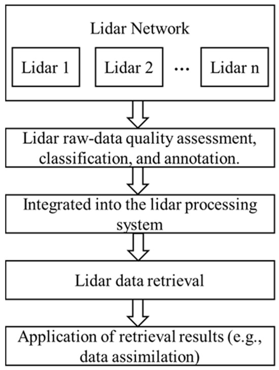
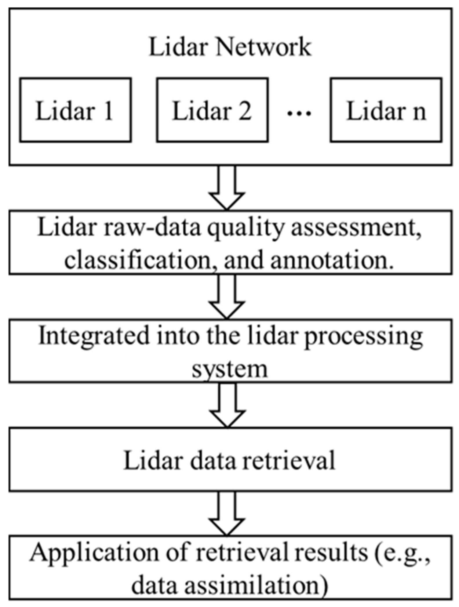
In the operation of the CARLNET, the collected lidar raw data is assessed, categorized based on quality and labeled. Then, the assessed data is integrated into the lidar data processing system. Subsequently, the results are applied to scientific research according to their quality, such as data assimilation. The CARLNET data-processing flowchart is shown in Figure 1.
Figure 1.
The data-processing flowchart for CARLNET.
2.2. Quality Assessment Methodology
In this study, three factors, signal saturation at near-range, Rayleigh fit and effective detection range, are used to assess the quality of lidar raw data.
2.2.1. Signal Saturation at Near-Range
Lidar signal saturation occurs when the strength of the echo signal received by the detector (e.g., a photomultiplier tube) exceeds the upper limit of its linear operating range. This results in the detector’s output signal no longer being proportional to the incident light intensity, and can even cause complete distortion or damage, thereby leading to invalid data retrieval. Consequently, the true structure of aerosols in the distorted signal range cannot be obtained, and the quantitative products, such as total aerosol optical depth (AOD), would be systematically underestimated. Therefore, the saturated data must be identified and flagged during application.
Signal saturation of atmospheric lidar is usually caused by the following reasons: (a) The emitted laser encounters strongly reflective objects, such as low clouds, dense fog and haze. This results in a very strong backscattered signal. (b) Contamination of optical lenses by dust, water vapor or water leakage, or freezing, resulting in strong reflected light entering the detection system. (c) The detector’s gain is set too high, putting it in a state of high sensitivity. When a medium-strength signal is encountered, the signal that would normally be detected at low gain may saturate the detector at high gain. (d) The detector has poor optical isolation, resulting in external scattered or reflected light entering it directly.
The setting of the threshold of near range is based on both physical and operational considerations. According to the lidar equation, the intensity of the lidar signal is inversely proportional to the square of the distance. Therefore, the closer the distance, the stronger the signal. A height of 1.5 km is the core area. The aerosol content within this height range is high, and the influence of human activities is significant. Additionally, at a height of 1.5 km, the geometric overlap factor of the lidars in the CARLNET reaches 1, meaning that the signal distortion below this height is mainly due to signal saturation rather than geometric obstruction. Therefore, the threshold at near range is set to be 1.5 km.
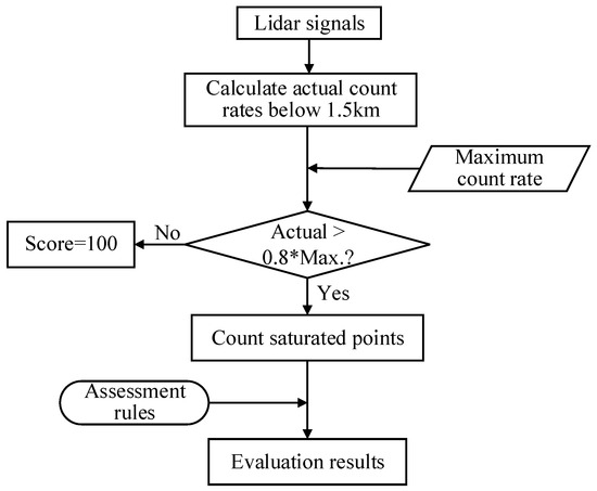
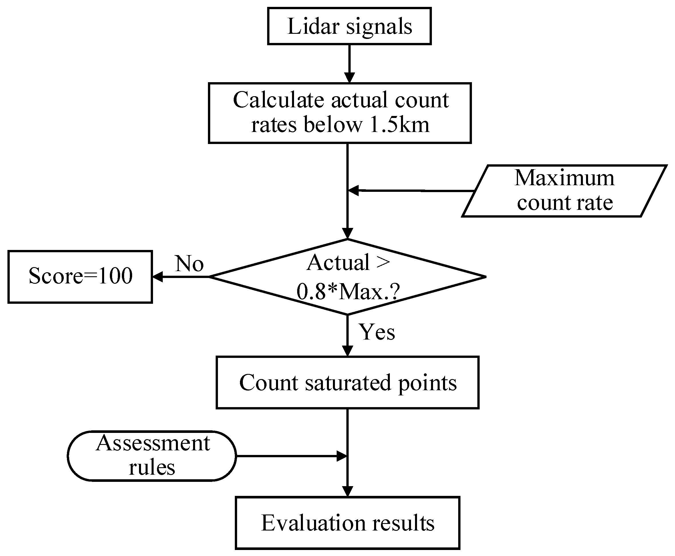
Figure 2 is the flowchart for assessing the saturation of the lidar signal. From the lidar equation, the echo power is inversely proportional to the square of the distance. In addition, the aerosols in the atmosphere are mainly distributed at near range; therefore, the lidar signal strength at near-range is larger and more easily saturated. We calculate the count rate of the signal and compare it with the maximum count rate of the acquisition card to analyze the signal. When the atmospheric lidar signal is saturated, the top of the signal curve will flatten out rather than continue to rise or reach a peak. In another case, the signal will drop abnormally, forming a depression where it should have continued to rise or peaked. These features are used to determine signal saturation.
Figure 2.
The flowchart for assessing the lidar signal saturation. “Actual” stands for actual count rate, and “Max.” stands for Maximum count rate. The asterisk (*) represents multiplication.
The scores of signal saturation at near-range are determined based on the number of saturation points. The more saturation points there are, the greater the impact on the retrieval results. A saturation point count of 1 is basically acceptable and can be given a passing score. We employ a straightforward linearly decreasing method to evaluate the score of signal saturation at near-range. Therefore, if the lidar signal at near-range (below 1.5 km) is saturated, when the number of saturated points is 1, the score is 60; when the number of saturated points is 2, the score is 45; when the number of saturated points is 3, the score is 30; when the number of saturated points is 4, the score is 15; and when the number of saturated points is greater than 4, the score is zero.
2.2.2. Rayleigh Fit
To obtain the quantitative values of aerosol/cloud during the lidar data retrieval, an absolute reference frame is required. The Rayleigh fit provides a theoretical benchmark of pure molecular scattering for aerosol/cloud retrieval, primarily through the theory of atmospheric molecular Rayleigh scattering [32,45].
The atmospheric echo signal of lidar is primarily made up of the atmospheric molecular Rayleigh scattering signal and the aerosol/cloud signal. In the aerosol-free region at far range, the echo signal of the lidar is mainly the atmospheric molecular Rayleigh scattering signal, and this section of the lidar signal should be consistent with the theoretical Rayleigh scattering signal.
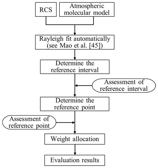
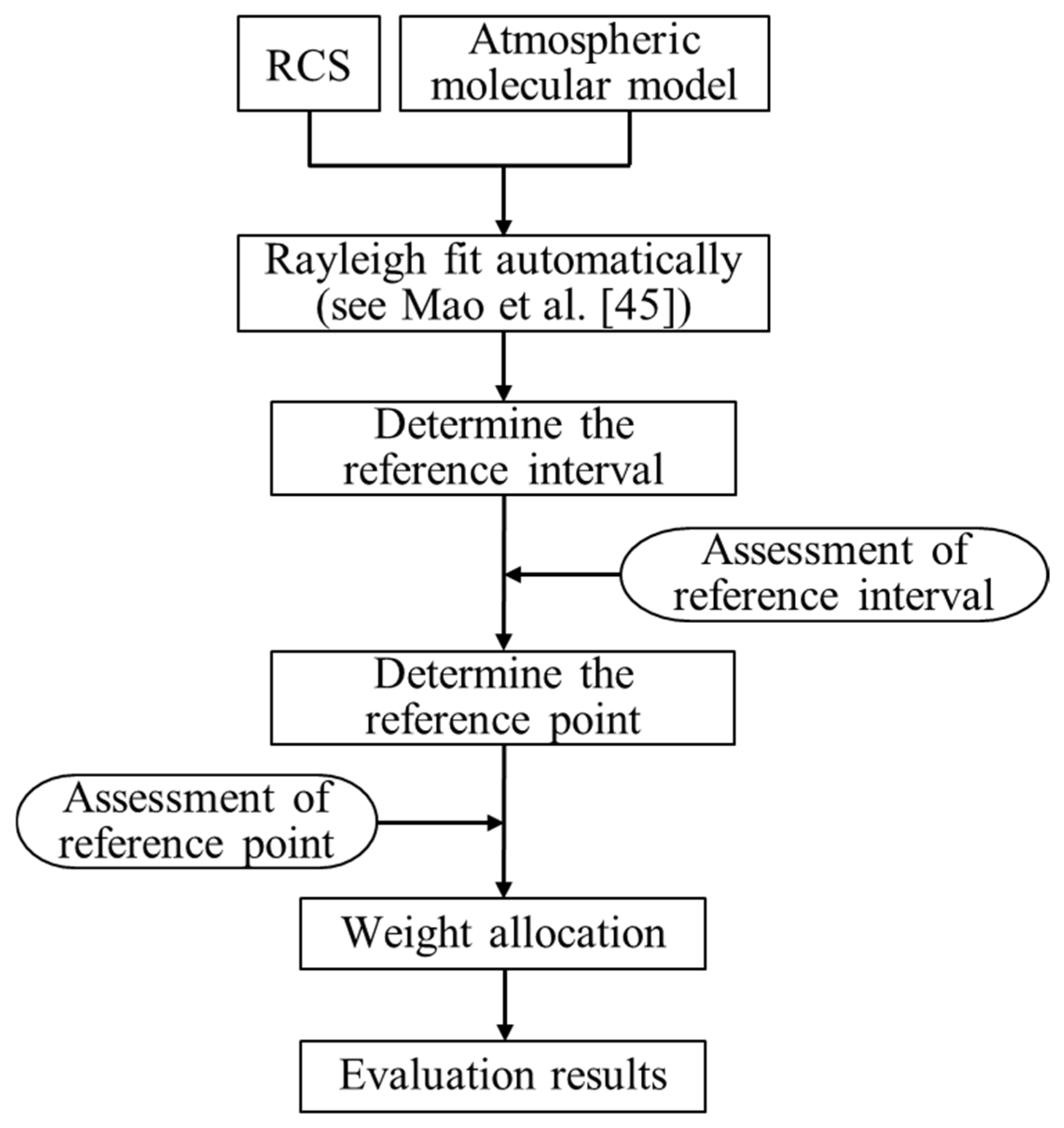
Rayleigh fit is a key factor in assessing lidar raw data quality. There are two main parameters that affect the Rayleigh fit, namely the Rayleigh fit reference interval and the reference point. The reference interval is typically chosen in aerosol-free regions. Signals with poor signal-to-noise ratios (SNR) or thin aerosols in the chosen reference interval will produce errors and then propagate into retrieval results. If the reference point is positioned too low, the aerosol structure above the reference point cannot be obtained, and the quantitative products, such as AOD, would be underestimated. Figure 3 shows the flowchart of the Rayleigh fit process. We calculate the range-corrected signals (RCS) of the lidar, as well as the atmospheric molecular scattering signal by standard atmospheric model. The aerosol-free region of the lidar signal is then searched for, and a Rayleigh fit is performed in that region. We developed rules for evaluating Rayleigh fit reference intervals and reference points, then scored them.
Figure 3.
The flowchart for evaluating the Rayleigh fit.
For the principles of selecting the reference interval and reference point for Rayleigh fit, we refer to Mao et al. [45]. The selection of the reference interval needs to ensure that the signal within it is sufficiently pure and has statistical representativeness. A short reference interval is prone to introducing systematic errors due to thin aerosol layers, while a longer one enhances statistical significance and reliability by averaging out such disturbances. A reference interval of 1 km is generally considered to be relatively reliable. Therefore, when the length of the reference interval is 0 km, 1 km, 3 km, or greater than or equal to 5 km, this item is scored 0, 60, 90 or 100 respectively. When the length of the reference interval is any other value, the score is obtained using linear interpolation. Aerosols are primarily distributed below 3 km, occasionally reaching up to 6 km (e.g., smoke or dust), whereas cirrus clouds are mainly distributed around 10 km, and aerosol content in the atmosphere decreases exponentially with height [46]. Therefore, when the position of the reference point is 0 km, 3 km, 6 km, 10 km, or greater than or equal to 20 km, the score for this item is 0, 60, 80, 90 or 100, respectively. Similarly, linear interpolation was used to obtain scores at alternative locations. Finally, the weighted average method was utilized to obtain a composite score for the Rayleigh fit process.
2.2.3. Effective Detection Range
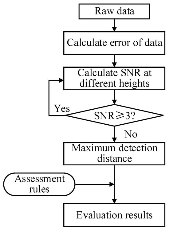
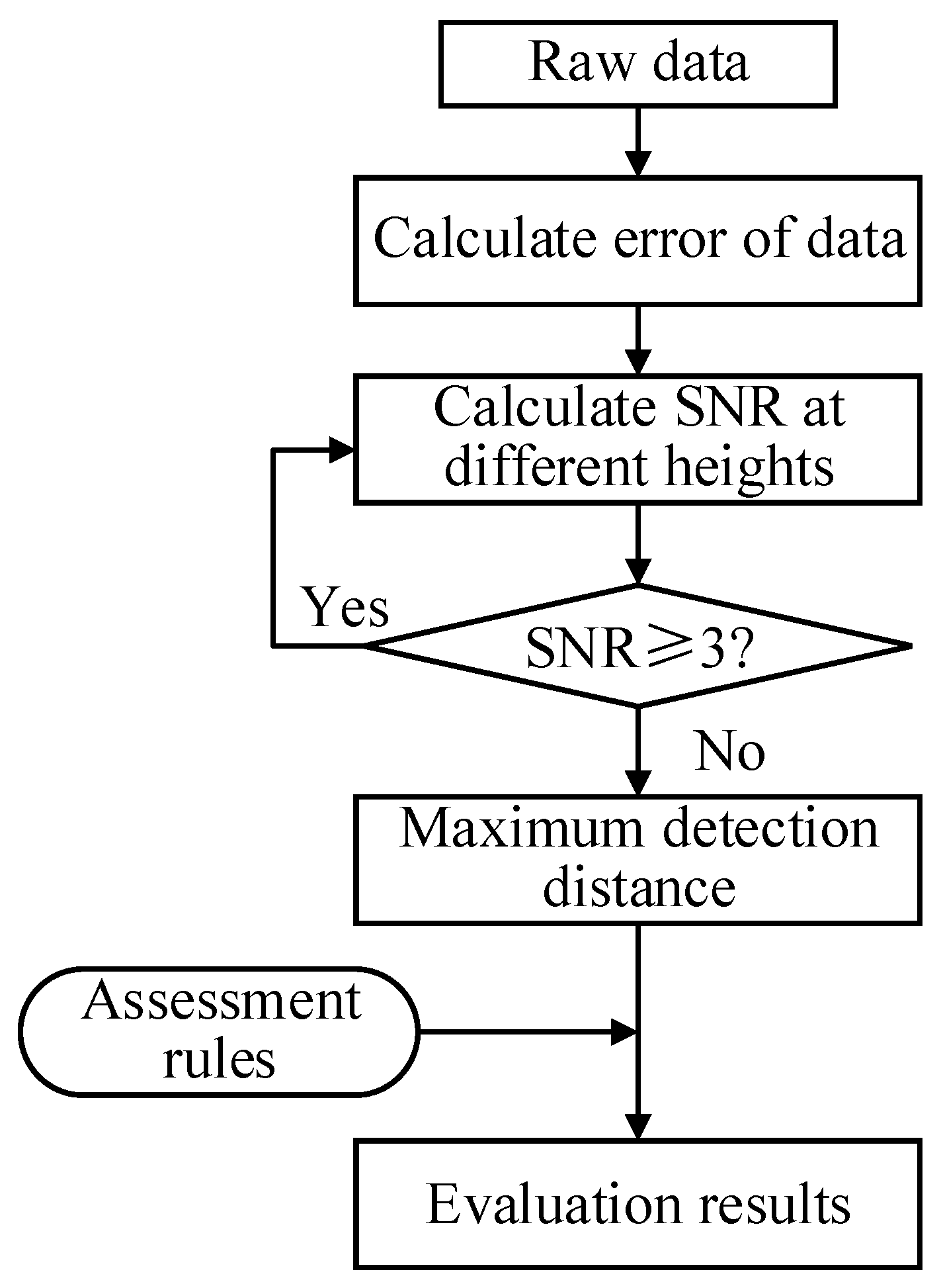
The effective detection range of aerosol lidar is a key indicator of its detection capability, which is usually defined as the distance at which the signal-to-noise ratio (SNR) is reduced to 3. The effective detection range is affected by the performance of the lidar system (e.g., emitting laser power, telescope diameter, optical efficiency, detector sensitivity, etc.) and the atmospheric conditions (e.g., clear sky, haze, low clouds, etc.). The effective detection range is related to the completeness of the retrieval results. A short effective detection range means that the signals at high range are overwhelmed by noise, and the retrieval results cannot contain the aerosol distribution above the effective detection range. Furthermore, the AOD would also be underestimated.
Figure 4 is a flowchart for assessing the effective detection range. Calculate the SNR of the lidar signal. Take 3 as the threshold and judge the effective detection range for SNR greater than or equal to 3 consecutively. Then evaluate the effective detection range.
Figure 4.
The flowchart for assessing the effective detection distance.
As the aerosol content decreases exponentially with height [46], the reduction in the effective detection range at near-range has a much greater impact on AOD than that at high-range. Therefore, the scoring gradient at near-range is greater than that at high-range. Therefore, when the effective detection range is 0 km, 5 km, 10 km, 15 km, or more than or equal to 20 km, the score is 0, 60, 80, 90, or 100, respectively. The scores for other distances were calculated using linear interpolation.
Once the scores for the three assessment factors above have been obtained, weights are assigned to them and the composite score for lidar raw data is obtained. Table 1 shows the lidar raw-data quality assessment factors and weight allocations. We have conducted relevant simulation analysis in Mao et al. (2024) [45] and determined the weights of the three factors based on the simulation results. Specifically, we assumed that the aerosol content in the atmosphere decreases exponentially with height [46]. We used the non-paralyzed model [43] to simulate the nonlinear response of the signal due to signal saturation. With the value of aerosol optical depth (AOD) as the target quantity, we simulated the influences of signal saturation at near-range, different Rayleigh fits, and different effective detection ranges on AOD. The simulation results show that the AOD deviation caused by signal saturation is greater than that from the other two factors. The AOD deviations resulting from variations in the Rayleigh fit and effective detection range are comparable. Therefore, the weights of the three factors were set as 0.4, 0.3, and 0.3 respectively.
Table 1.
Lidar raw-data quality assessment factors and weight allocation.
3. Results
This study analyzes and discusses the proposed quality assessment method, focusing on three aspects: (a) the quality assessment for lidar raw data under different weather scenarios; (b) the identification of system hardware issues based on the results of raw-data quality assessment; (c) the statistical analysis of the raw-data quality of the CARLNET.
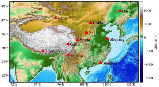
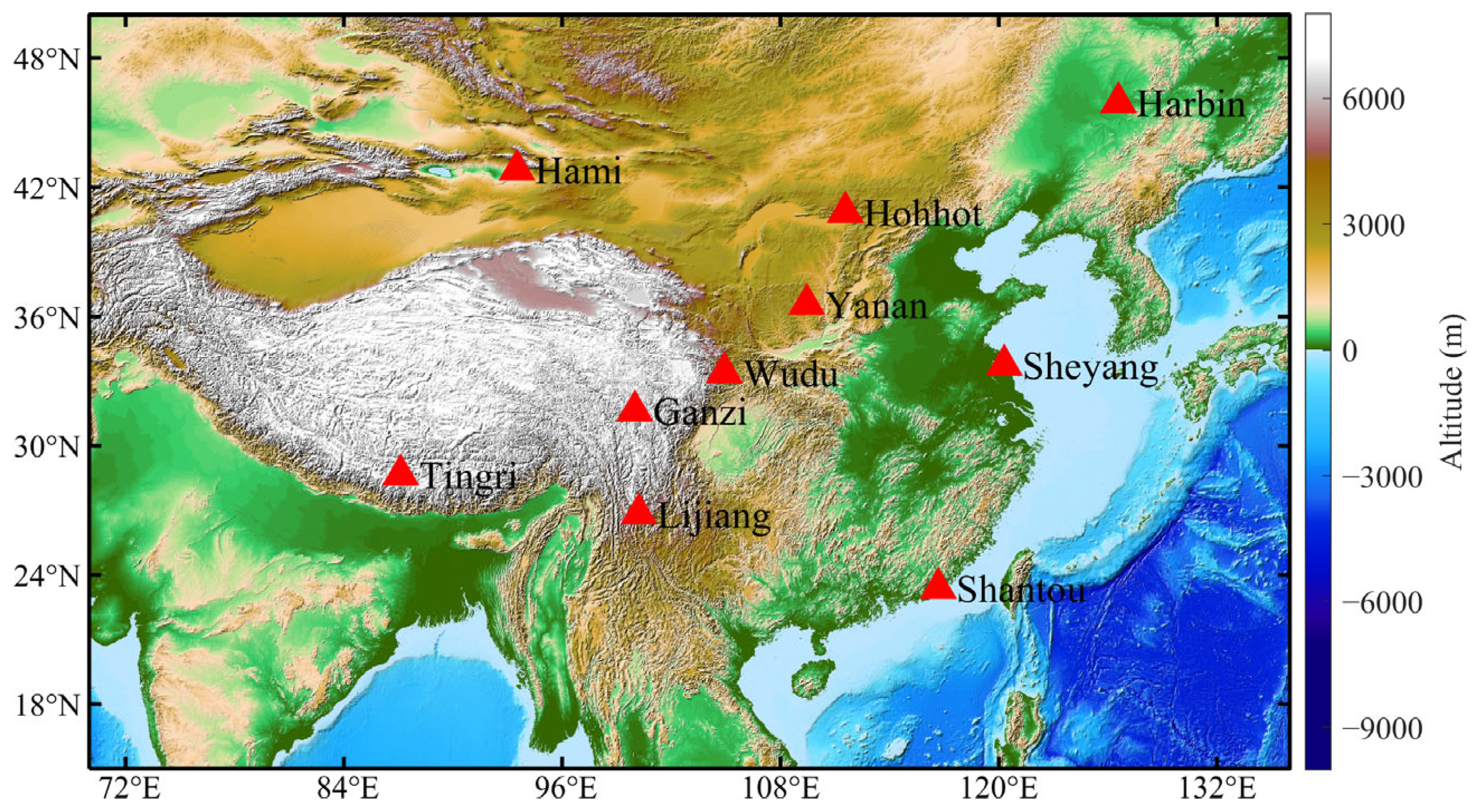
For the three aspects discussed above, ten representative observation sites are selected, and the raw data is assessed with the proposed algorithm. Figure 5 shows the distribution of representative lidar stations. As shown in the figure, the selected lidar stations are distributed across a wide area, covering a longitude range of 87.1° to 126.6° and a latitude range of 23.4° to 45.9°. The lidar sites are located in both high-altitude and low-altitude regions, and the climate encompasses desert fringes, plateau regions, grasslands, plains and coastal areas.
Figure 5.
The distribution of representative lidar stations. The base map is a digital elevation model (DEM).
Table 2 lists the basic information of the ten observation sites (See Figure 5), including lidar site, altitude and the data time used in this study. The raw data from the Ganzi, Wudu and Hohhot sites was used to analyze the capability of the quality assessment method under different weather scenarios. The Dingri and Harbin sites served as examples to identify the system hardware issues based on the results of the raw-data assessment. Data from Hami, Yan’an, Lijiang, Sheyang, and Shantou stations were used for statistical analysis of the quality of lidar raw data.
Table 2.
Basic information on representative observation sites.
3.1. The Influence of Different Observation Scenes
Weather conditions directly affect the lidar observation results. The quality of lidar raw data varies under different weather conditions. We selected three typical weather conditions for analysis: sunny, cloudy, and dusty weather.
3.1.1. Sunny Weather
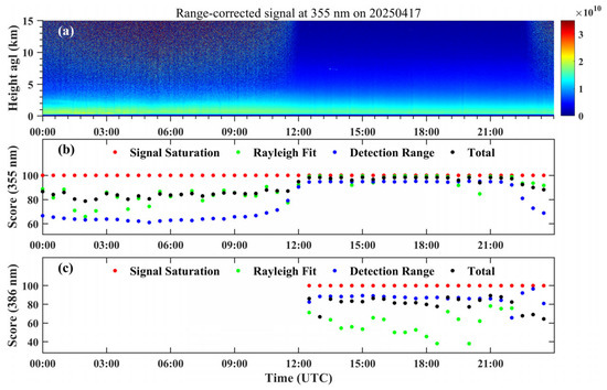
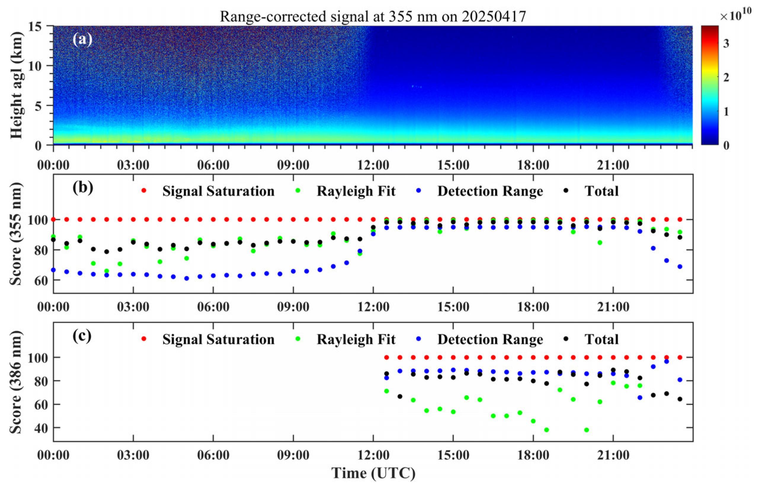
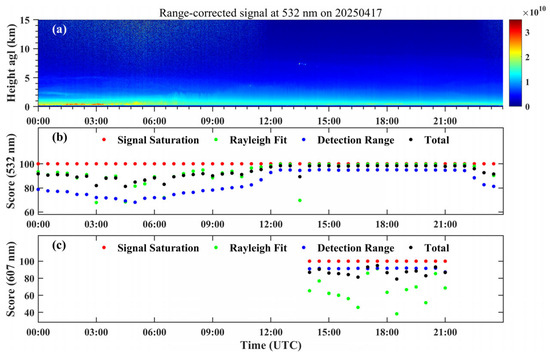
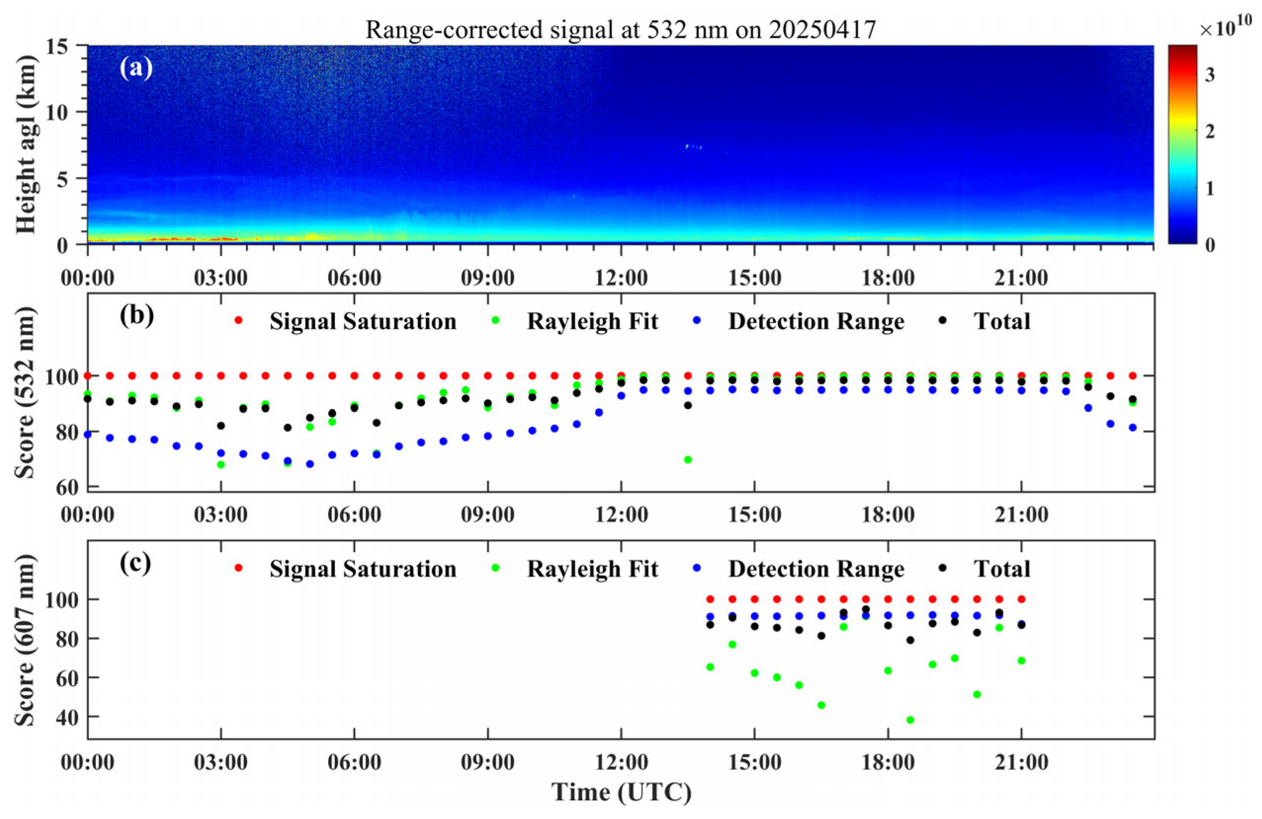
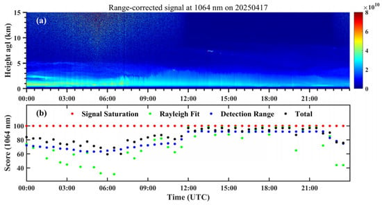
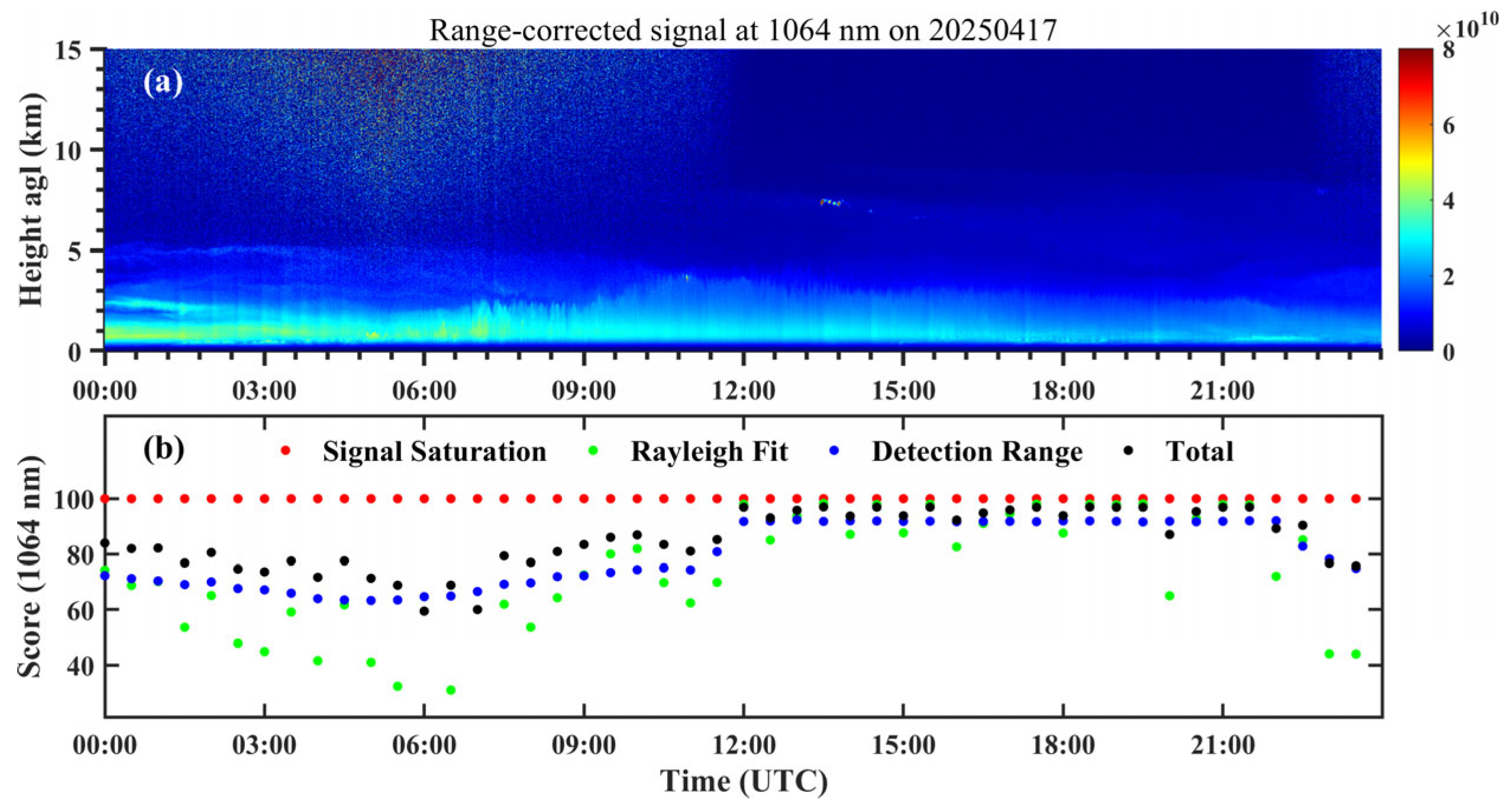
We select a sunny day at the Ganzi site on 17 April 2025 as an example to analyze lidar raw-data quality at wavelengths of 355 nm, 386 nm, 532 nm, 607 nm and 1064 nm. Figure 6, Figure 7 and Figure 8 show the range-corrected signal (RCS) and the scoring results at Ganzi station. In this example, the atmosphere is relatively clean with no clouds. The distribution of aerosols is relatively sparse, with the majority concentrated below 3 km.
Figure 6.
Scenario of sunny weather at Ganzi station on 17 April 2025. (a) RCS at 355 nm, (b) score of lidar raw data at 355 nm, (c) score of lidar raw data at 386 nm.
Figure 7.
Scenario of sunny weather at Ganzi station on 17 April 2025. (a) RCS at 532 nm, (b) score of lidar raw data at 532 nm, (c) score of lidar raw data at 607 nm.
Figure 8.
Scenario of sunny weather at Ganzi station on 17 April 2025. (a) RCS at 1064 nm, (b) score of lidar raw data at 1064 nm.
As shown in Figure 6, the data at 355 nm and 386 nm did not saturate, with both scores being 100. The scores of effective detection distance for the data at 355 nm were less than 80 between 00:00 and 12:00 UTC, approaching 100 between 12:00 and 22:00 UTC. Clearly, the score for this item is significantly higher at night than during the day. The score of the Rayleigh fit shows the same pattern. This is because the background noise during the daytime is much greater than that at nighttime.
For the Raman signal at 386 nm, considering that the background noise is relatively high during the day and the signal is weak, currently, only the Raman signals at night have been scored. On this sunny day, the scores of effective detection range for Raman signal at 386 nm are relatively high, exceeding 80 for most of the time. The Rayleigh fit scores for 386 nm are relatively low relative to the effective detection range, but Rayleigh fitting is achievable throughout this time. The total scores for the data at 355 nm were all above 80, as were the scores for the 386 nm for most of the time, indicating good data quality.
Figure 7 shows the scores of the signal at 532 nm and 607 nm. The raw signals at 532 nm and 607 nm are not saturated. The scoring situation and patterns at 532 nm are basically similar to those of the 355 nm signal. The effective detection range of the Raman signal at 607 nm is quite far, and this score is above 80. The reference interval and reference point can also be found for the Raman signal at 607 nm. The total scores for the data at 532 nm were all above 80, as were the scores for the 607 nm for most of the time, indicating good data quality.
Figure 8 shows the scores of lidar data at 1064 nm. We can see that this signal is not saturated. At night, the scores for effective detection range and Rayleigh fit are better than those during the day. The total score of data at 1064 nm exceeded 60 during daytime and approached 100 at nighttime.
Overall, under sunny weather conditions, the total scores of each detection channel were relatively high. The data quality is relatively good.
3.1.2. Cloudy Weather
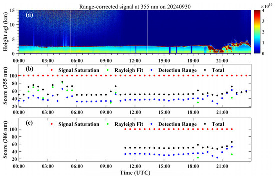
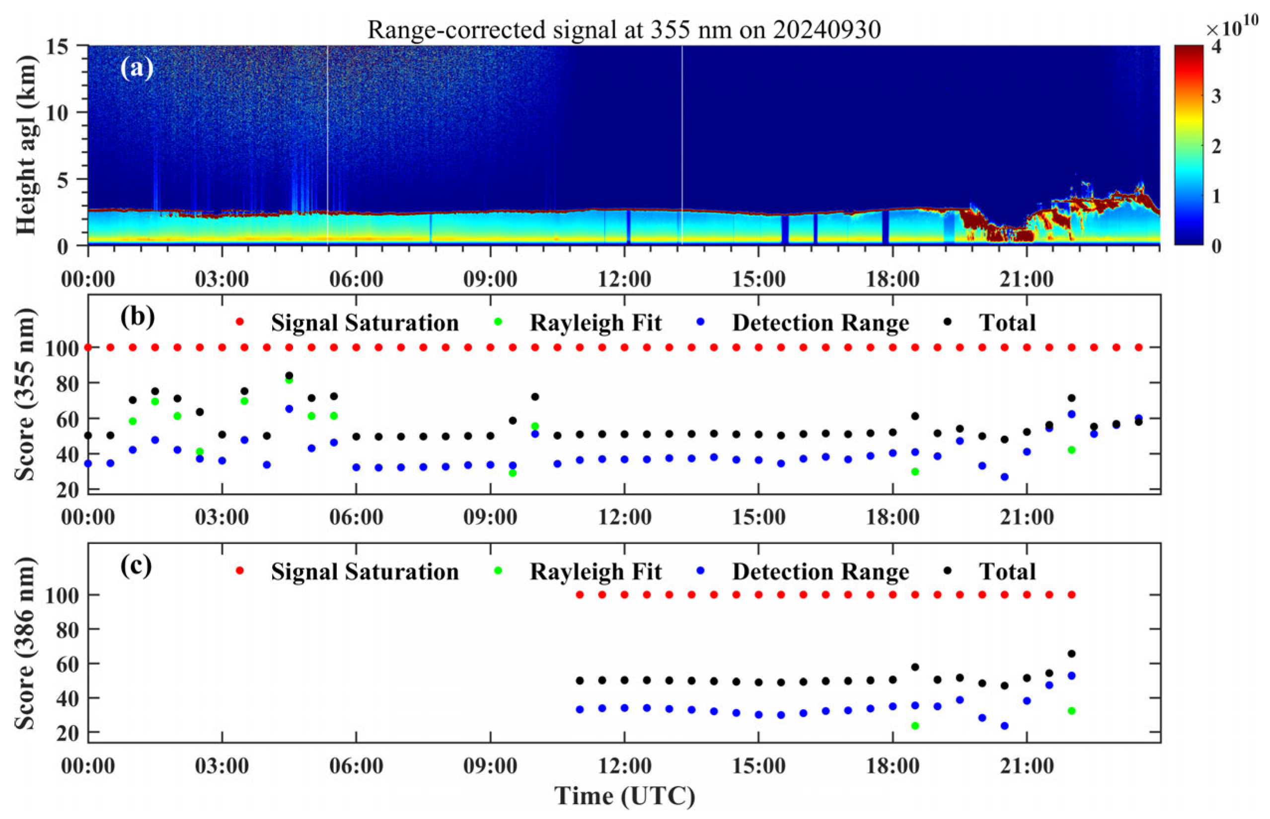
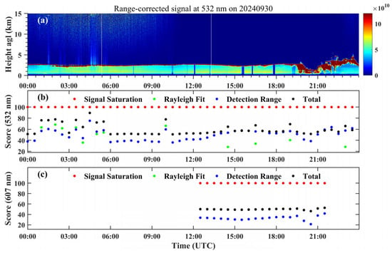
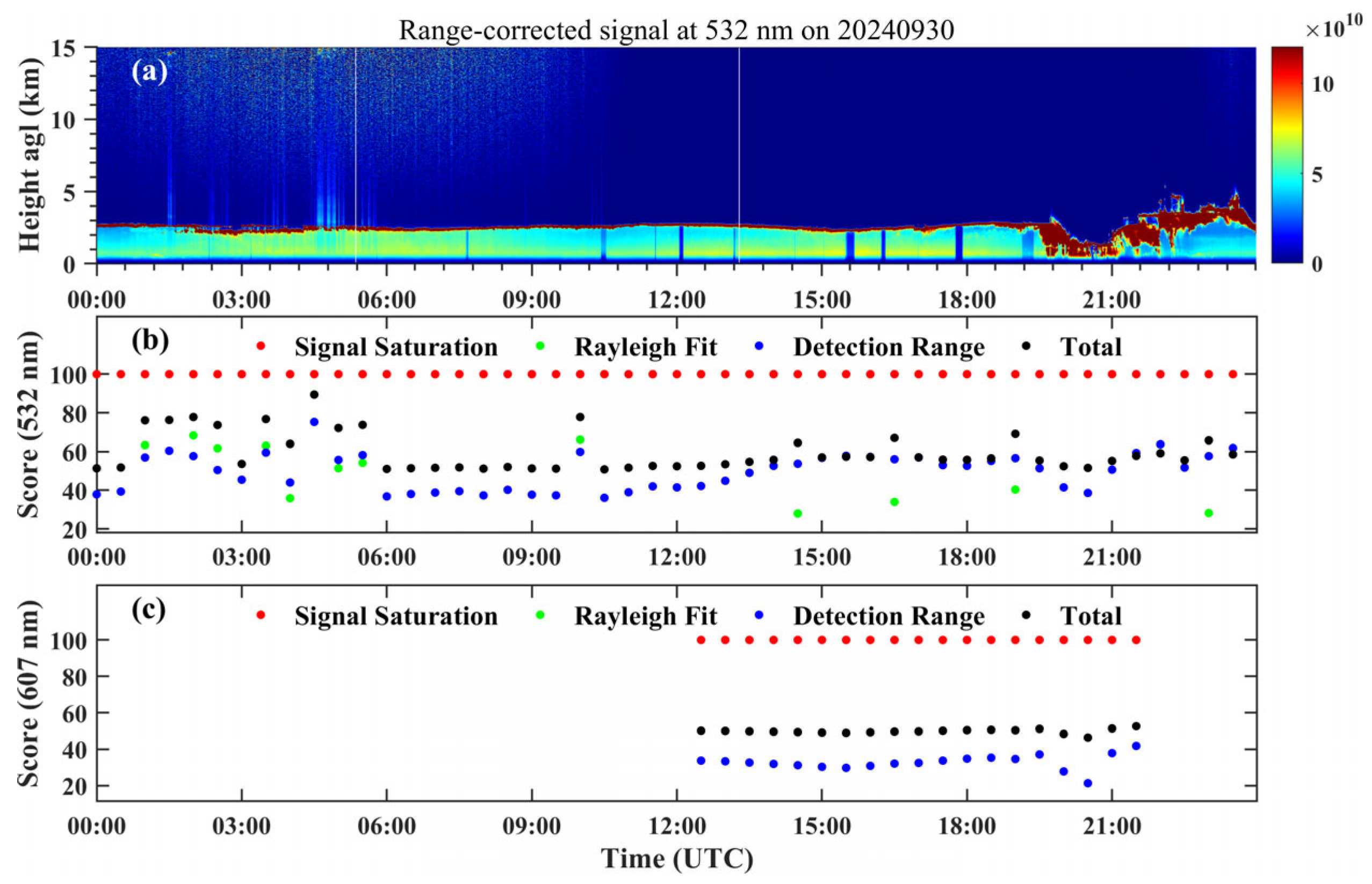
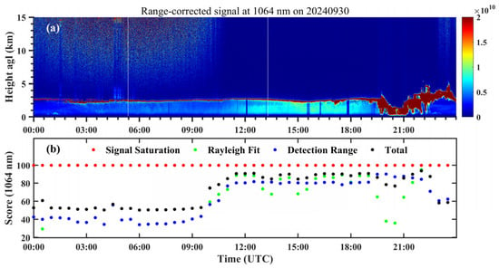
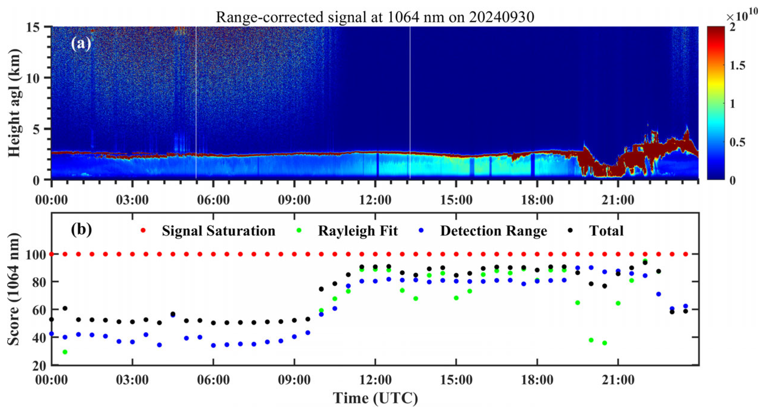
We select a cloudy day at the Wudu site on September 30, 2024, as an example to analyze lidar raw-data quality at 355 nm, 386 nm, 532 nm, 607 nm and 1064 nm. Figure 9, Figure 10 and Figure 11 show the RCS and the assessment results at Wudu station. In this scenario, a low cloud can be seen approximately 3 km away, which makes the laser not penetrate the clouds most of the time.
Figure 9.
Scenario of cloudy weather at Wudu station on 30 September 2024. (a) RCS at 355 nm, (b) score of lidar raw data at 355 nm, (c) score of lidar raw data at 386 nm.
Figure 10.
Scenario of cloudy weather at Wudu station on 30 September 2024. (a) RCS at 532 nm, (b) score of lidar raw data at 532 nm, (c) score of lidar raw data at 607 nm.
Figure 11.
Scenario of cloudy weather at Wudu station on 30 September 2024. (a) RCS at 1064 nm, (b) score of lidar raw data at 1064 nm.
In Figure 9, the raw signals at 355 nm and 386 nm are not saturated. Before 06:00, some laser beams penetrated below the cloud base. During this time, the effective detection distance score was higher than that during other periods, enabling Rayleigh fitting to be achieved. The scores of effective detection distance for 355 nm signal below 40, and Rayleigh fitting cannot be achieved for most of the time. Except for a few time periods where Rayleigh fitting could be achieved, the total score for the data at 355 nm remained below 60 for most of the time, indicating poor data quality.
For data at 386 nm, before 21:00, the effective detection range score is less than 40. Rayleigh fitting can only be achieved at two time points. The total scores for lidar raw data at 386 nm were less than 60 for most of the time, indicating poor data quality.
Figure 10 shows the scores of lidar data at 532 nm and 607 nm. The raw data at 532 nm and 607 nm were not saturated. The scoring situation and patterns at 532 nm are basically similar to those of the 355 nm signal. The score of the effective detection range decreased significantly after 6:00 due to the laser’s inability to penetrate the cloud. Rayleigh fitting cannot be achieved most of the time. Except for a few time periods where Rayleigh fitting could be achieved, the total score for the data at 532 nm remained below 60 for most of the time, indicating poor data quality.
For 607 nm, for most of the time, the effective detection distance score was less than 40, and Rayleigh fitting was not achieved at any time. During this period, the total score for the data at 607 nm remained consistently below 60, indicating poor data quality.
Figure 11 shows the RCS and scores of lidar data at 1064 nm. We can see that there is no saturation of the signal. As the shorter the wavelengths, the stronger the scattering, the 1064 nm wavelength exhibits greater atmospheric penetration compared to 355 nm and 532 nm. As shown in the figure, during daytime, the effective detection distance score for the 1064 nm data was relatively low (around 40), and failed to achieve Rayleigh fitting except at one time point. At nighttime, the effective detection distance score for 1064 nm data improved significantly to approximately 80, with nearly all cases achieving Rayleigh fitting.
Compared with the lidar raw data at 355 nm and 532 nm, the total score for 1064 nm data during daytime remains poor, with most scores below 60. However, at night, the total score for 1064 nm data significantly improves, exceeding 80 for most time periods.
Overall, the method proposed in this study can distinguish the poor data quality under low-cloud conditions and identify quality differences across data at different wavelengths.
3.1.3. Dust Weather
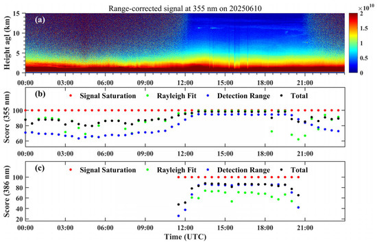
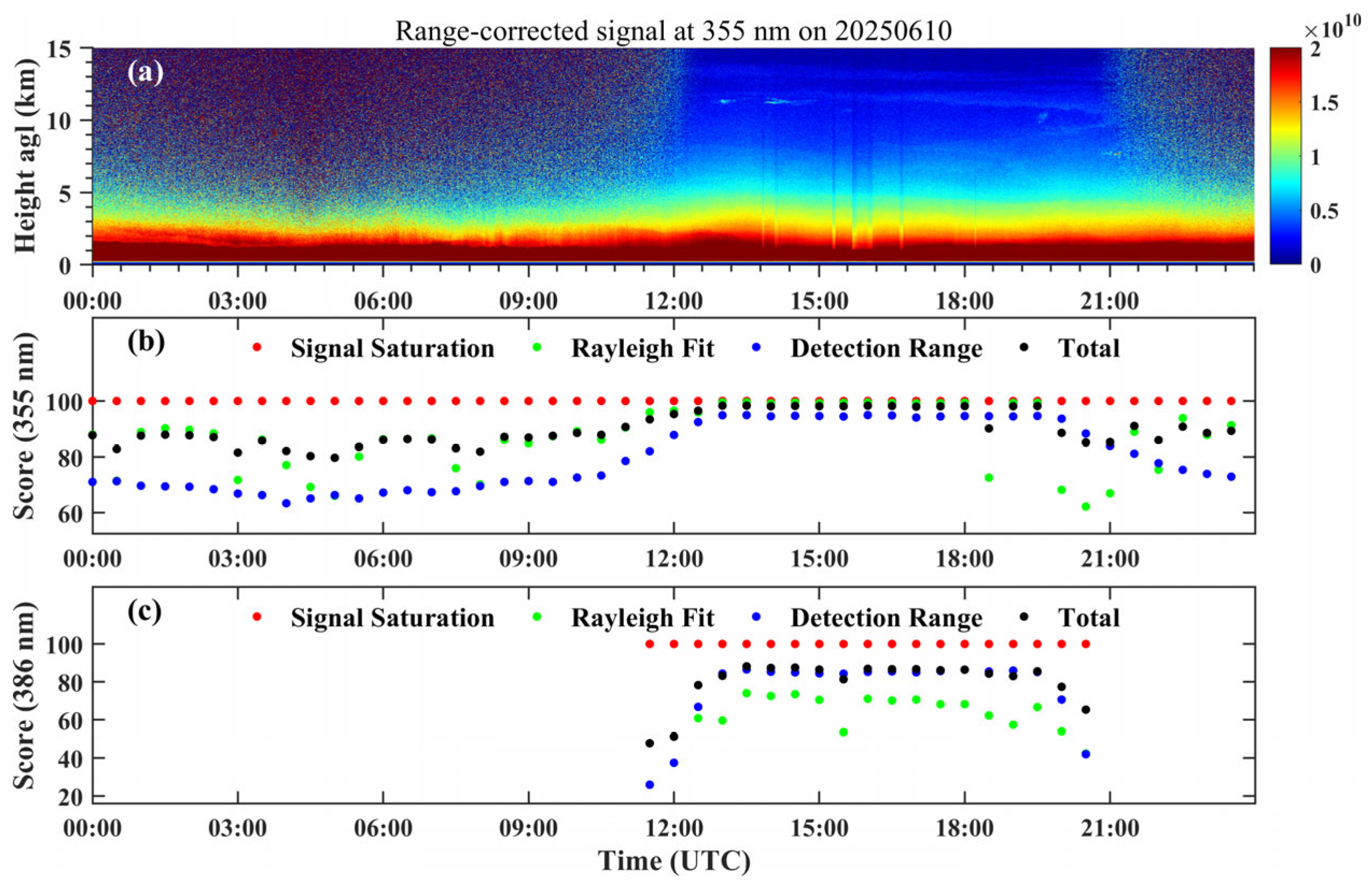
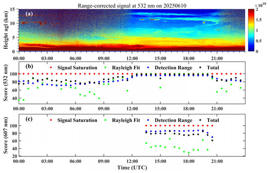
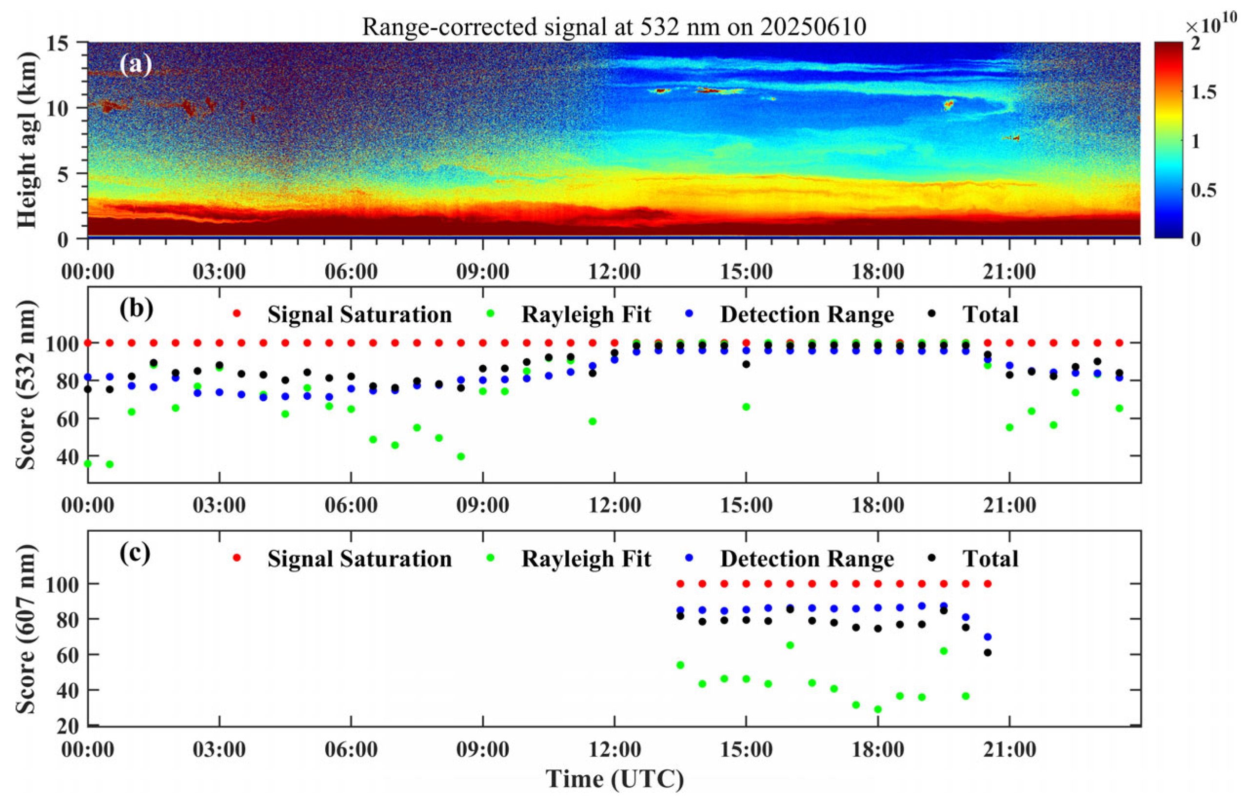
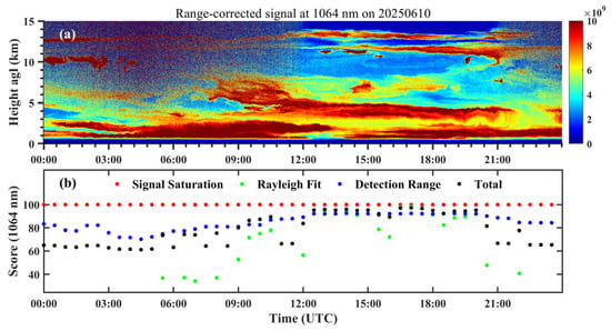
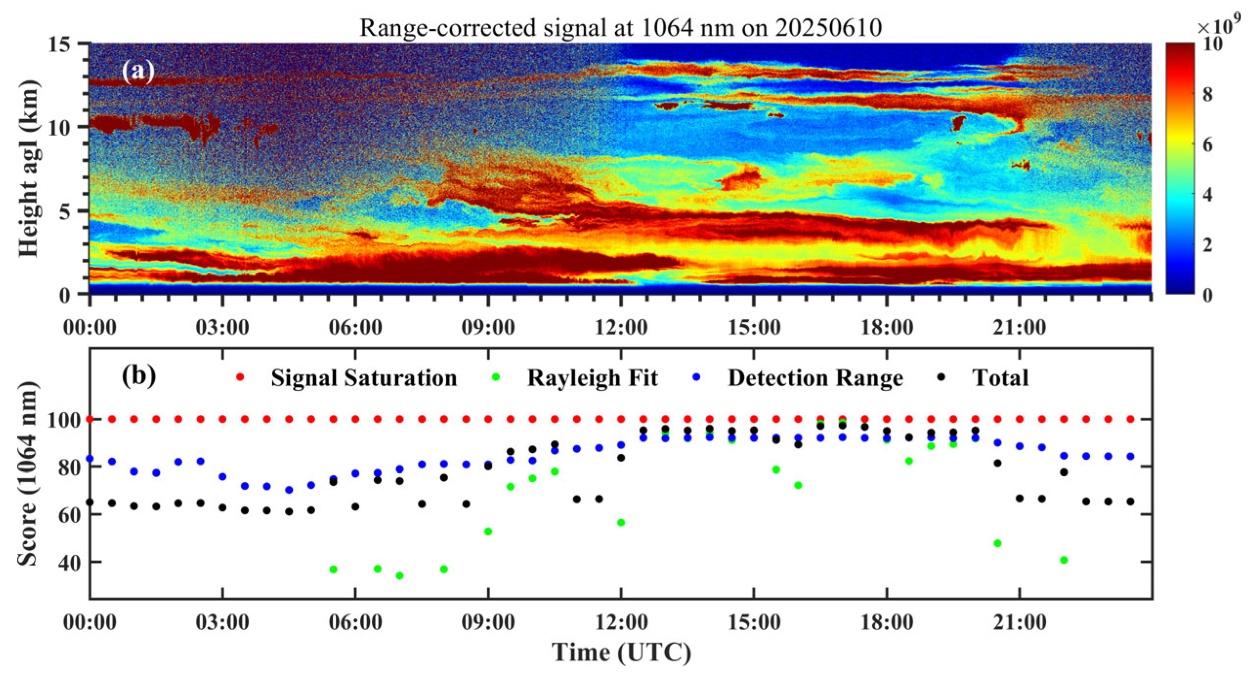
We select dusty weather at the Hohhot site on June 10, 2025, as an example to analyze lidar raw data at 355 nm, 386 nm, 532 nm, 607 nm and 1064 nm. Figure 12, Figure 13 and Figure 14 show the scenario of dusty weather at Hohhot station and the scoring results. In this scenario, there are many aerosols in the atmosphere, and the layers are clearly distinguishable. Compared to the signal at 355 nm, the signals at 1064 nm and 532 nm have a stronger ability to identify aerosols and can detect more abundant information.
Figure 12.
Scenario of dust weather at Hohhot station on 10 June 2025. (a) RCS at 355 nm, (b) score of lidar raw data at 355 nm, (c) score of lidar raw data at 386 nm.
Figure 13.
Scenario of dusty weather at Hohhot station on 10 June 2025. (a) RCS at 532 nm, (b) score of lidar raw data at 532 nm, (c) score of lidar raw data at 607 nm.
Figure 14.
Scenario of dusty weather at Hohhot station on 10 June 2025. (a) RCS at 1064 nm, (b) score of lidar raw data at 1064 nm.
From Figure 12, the raw data at 355 nm and 386 nm are not saturated. The effective detection distance score for data at 355 nm is below 80 during daytime and approaches 100 at night. Similarly, the Rayleigh fit score is low during the day and high at night. The total scores for the data at 355 nm are almost all above 80, indicating good data quality.
The effective detection distance scores for the data at 386 nm mostly exceeded 80, the Rayleigh fit scores mostly exceeded 60, and the total scores mostly exceeded 80, indicating good data quality.
The scoring results of the data at 532 nm are similar to those of the 355 nm signal, as can be seen in Figure 13. The difference is that the 532 nm signal detects more aerosol information, and the Rayleigh fit score is relatively lower. The effective detection distance scores for the data at 607 nm mostly exceeded 80, the Rayleigh fit scores mostly fell below 60, and the total scores were mostly less than 80, indicating moderate data quality.
In Figure 14, a relatively rich aerosol layer was detected by the signal at 1064 nm. Overall, the scores of the effective detections were below 80 for most daytime and above 80 at nighttime. However, due to the high concentration of aerosols within 3 km and the relatively high background noise during the daytime, the Rayleigh fitting was not achieved for data at 1064 nm from 00:00 to 05:00 UTC, and the score of the Rayleigh fit was low from 06:00 to 09:00 UTC. During the nighttime, the score of the Rayleigh fit significantly improved. The total scores for the data at 1064 nm were nearly below 80 during the daytime and above 80 at nighttime, indicating moderate data quality at daytime and good data quality at nighttime.
In the dusty weather conditions, the different wavelength signals (355 nm, 532 nm and 1064 nm) of the same lidar have varying capabilities in detecting particles; therefore, the raw-data quality at different wavelengths also differs. The quality assessment method proposed in this study can effectively distinguish the quality of the raw data.
3.2. Hardware Issues Reflected by Assessment Results
The lidar raw-data scores can also indicate certain hardware issues. If the assessment results are persistently abnormal after weather factors have been ruled out, a root cause analysis can be carried out to identify the issues and rectify the hardware.
3.2.1. Optical-Axis Misalignment
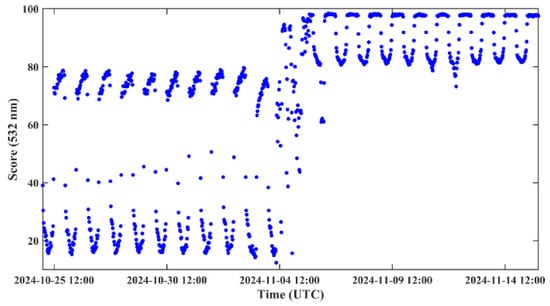
Figure 15 shows the score of the effective detection range at Tingri station. During analysis of lidar signal scores, it was found that the effective detection distance score for the data at 532 nm remained below 30 for most of the daytime, and remained below 80 even at nighttime between 25 October 2024 and 14 November 2024.
Figure 15.
Score of effective detection range at Tingri station from 25 October 2024 to 14 November 2024.
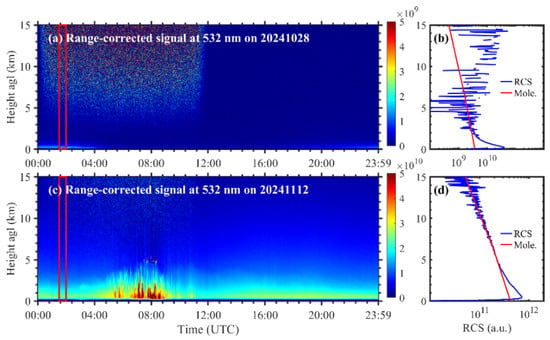
Figure 16a shows the lidar data at 532 nm on 28 October 2024 at Tingri station. As the figure shows, it was a cloudless day. Figure 16b shows the RCS profile for the time interval from 01:00 to 01:30 UTC. As can be seen, the signal-to-noise ratio is poor, with the effective detection range extending only to around 2 km.
Figure 16.
Timeseries of signal at Tingri station. (a) RCS at 532 nm on 28 October 2024, (b) profile of RCS between 01:00 and 01:30 on 28 October 2024, (c) RCS at 532 nm on 12 November 2024, (d) profile of RCS between 01:00 and 01:30 on 12 November 2024.
A low detection range is typically caused by factors such as weather conditions, the laser source, or optical-axis misalignment. Through Figure 16a,b, we ruled out weather as a contributing factor. Through on-site investigation, it was found that the misalignment between the laser emission direction and the optical axis of the telescope caused this issue. This is because temperature variations exert a certain influence on both the laser beam axis and the positioning of lenses within the receiving system. During prolonged operation of the system, these deviations accumulate to a significant degree that cannot be ignored.
After adjusting the optical axis of the laser beam, the observation results showed a significant improvement. Figure 16c shows the spatial-temporal of the data observed on 12 November 2024, and Figure 16d shows the RCS profile between 01:00 and 01:30. The SNR has increased markedly, with the effective detection range score reaching approximately 10 km. As shown in Figure 15, the effective detection distance scores for both daytime and nighttime at this site exceeded 80 after 5 November 2024.
3.2.2. Signal-Receiving Issue
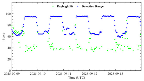
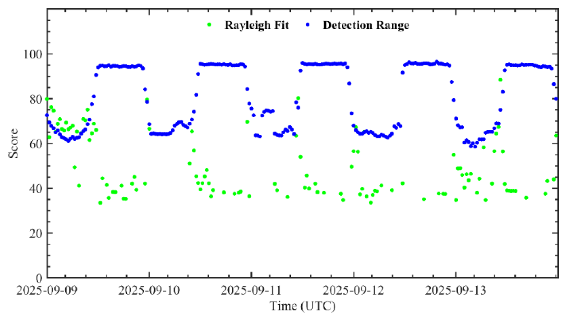
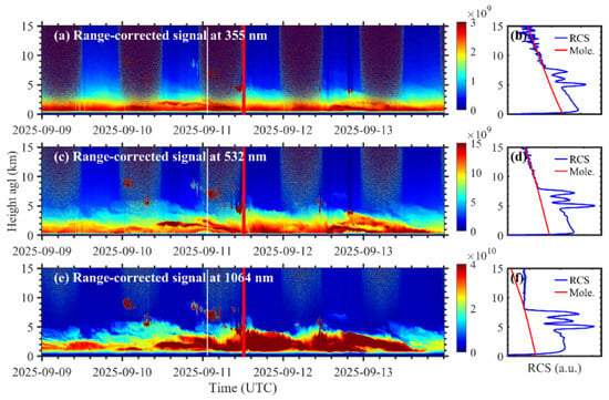
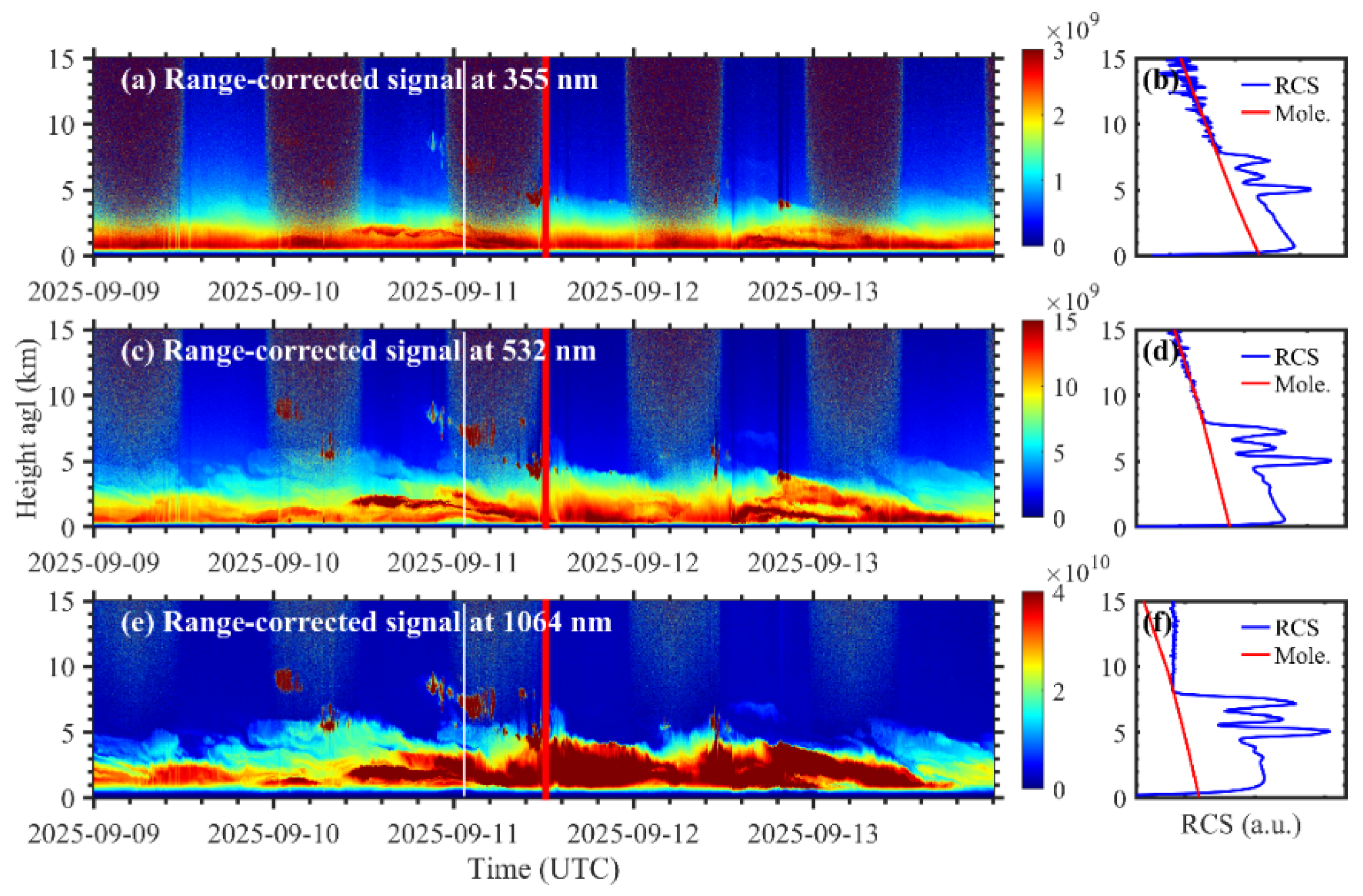
Figure 17 is the timeseries of lidar raw data and scores at 1064 nm at Jiuquan station between 9 September and 14 September 2025. As shown in the figure, the effective detection distance scores for the data at 1064 nm were relatively high (around 95), particularly at nighttime. However, the Rayleigh fit scores at nighttime were comparatively low (around 40). As shown in Figure 18a,c,e, aerosols were primarily concentrated below 5 km on these days; that is, the issues were not weather-related, which indicated a potential issue.
Figure 17.
Timeseries of lidar raw data and scores at Jiuquan station between 9 September and 14 September 2025.
Figure 18.
RCS at Jiuquan station between 9 September and 14 September 2025. (a,c,e) RCS at 355 nm, 532 nm and 1064 nm, respectively, (b,d,f) profile of RCS at 12:00 on 14 September 2025 at 355 nm, 532 nm and 1064 nm, respectively.
Figure 18a,c,e were the RCS at Jiuquan station between 9 September and 14 September 2025 at 355 nm, 532 nm and 1064 nm, respectively. We selected 11 September 2025, at 12:00 UTC and displayed the profile for 355 nm, 532 nm, and 1064 nm (see Figure 18b,d,f).
The results show that the RCS profiles at 355 nm and 532 nm are clear above 7 km, and the Rayleigh fit shows well. However, the profile of the 1064 nm signal shows significant anomalies above 7 km. It can effectively identify potential issues. Subsequent inspections revealed that the issue was caused by an increase in the detector’s dark counts in the 1064 nm channel due to aging.
3.3. Statistical Analysis of Lidar Data Quality
3.3.1. Timeseries of Score at Typical Observation Sites
The lidar raw-data quality assessment method proposed in this study can be used to assess the temporal variation in raw-data quality at observation sites. Five observation sites, Hami in Xinjiang, Yan’an in Shanxi, Lijiang in Yunnan, Sheyang in Jiangsu and Shantou in Guangdong, were set as examples.
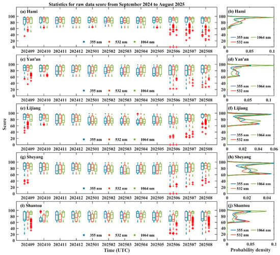
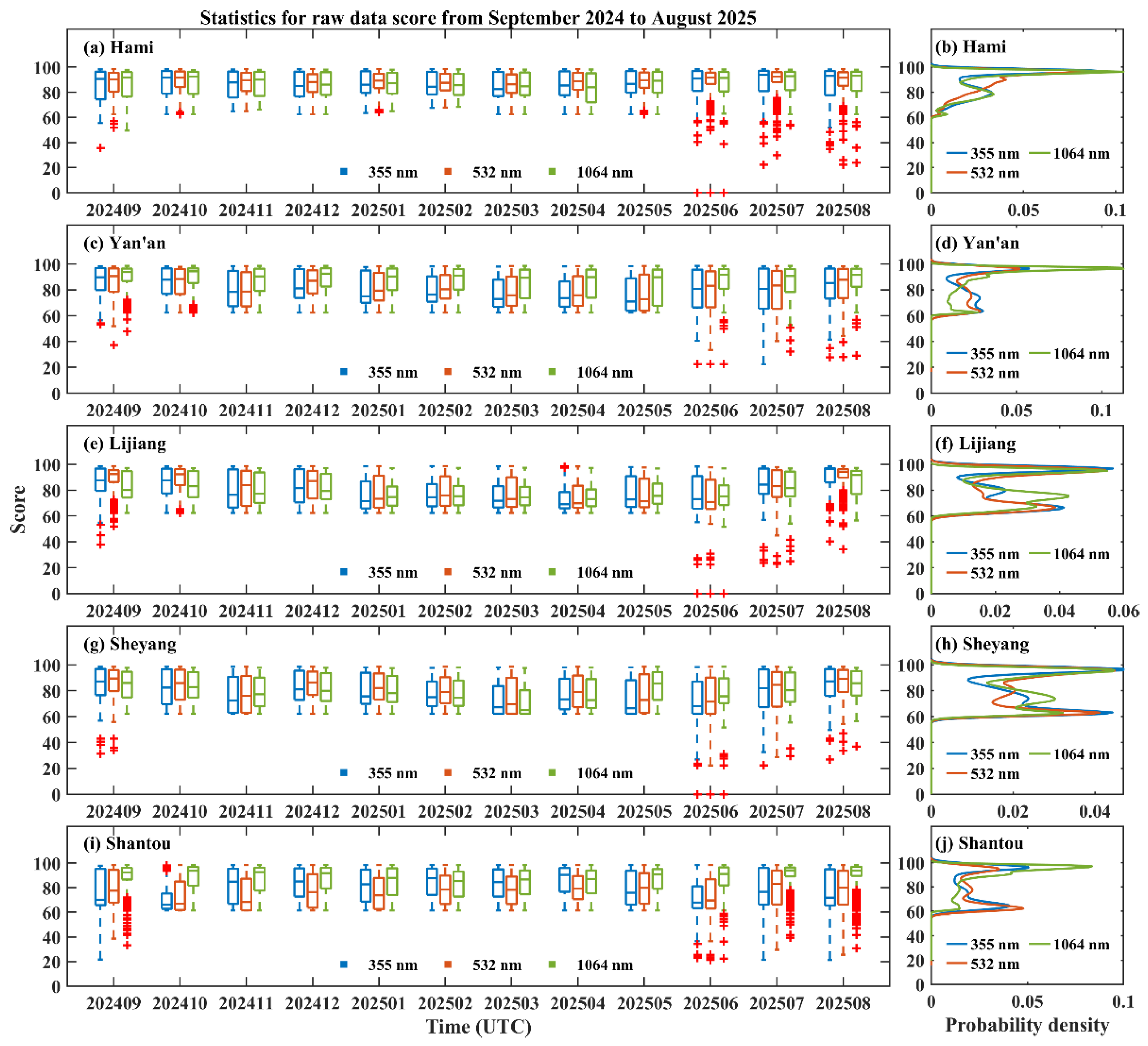
Figure 19 shows the score statistical result from 1 September 2024 to 31 August 2025 for the five sites, while quality assessments were conducted every 5 min (assessment intervals can be adjusted as needed). Figure 19a,c,e,g,i show box plots of the monthly data scores at 355 nm, 532 nm, and 1064 nm, which could be used to analyze seasonal variations in data quality. Figure 19b,d,f,h,j present the corresponding probability density distributions, which reflect the overall data quality of the five sites for this year.
Figure 19.
Timeseries of lidar raw data score. Box plots and probability density distributions of (a,b) Hami station, (c,d) Yan’an station, (e,f) Lijiang station, (g,h) Sheyang station, and (i,j) Shantou station, respectively. The blue, orange, and green represent 355 nm, 532 nm, and 1064 nm, respectively.
As shown in Figure 19, the score distribution at the Hami site is highly concentrated, with both the median and mean scores (see Table 3) at the 355 nm, 532 nm, and 1064 nm exceeding 80. This is primarily due to the relatively clean atmosphere in the Hami region, which is characterized by clear sky and low contents of aerosols. Of these five observation sites, the statistical samples in September 2024 and from June to August 2025 contained a relatively high number of outliers (red crosshair in Figure 19). Compared to other months, the score distribution is relatively scattered. This is because cloud cover and rainy weather are more frequent from June to September. These conditions can affect lidar raw data quality, resulting in outliers in the data scores.
Table 3.
The monthly average scores for five observation sites.
The probability density distribution function reveals that the data quality at 355 nm, 532 nm and 1064 nm was consistent for the same lidar. Each probability density function exhibited two distinct peaks, reflecting the differing quality of raw data during daytime and nighttime. At the Hami and Yan’an stations, the peaks with scores above 80 far exceeded the peaks below 80, while the differences between the two peaks were not significant at the remaining three stations. This suggested that the overall data quality at the Hami and Yan’an stations was better than at the other three stations during the observation period.
Table 3 shows the monthly average scores for five observation sites. From September 2024 to August 2025, the average scores for 355 nm, 532 nm, and 1064 nm were all larger than 80 at the Hami, Yan’an, and Lijiang stations, indicating good data quality. The average scores at the Sheyang and Shantou stations were lower, with some scores below 80. This is because Sheyang and Shantou are coastal cities that experience more cloudy weather.
In addition, Table 3 indicates that the months with lower scores are primarily concentrated in September 2024 and June–August 2025. During these four months, except for the Hami station, the average scores for wavelengths of 355 nm, 532 nm, and 1064 nm at the other four stations were not all greater than 80. Notably, at the Lijiang station, the data scores for all three wavelengths (355 nm, 532 nm and 1064 nm) were below 80 during these four months. As mentioned above, the cloud cover and rainy weather are more frequent in these months.
The box plots and probability density distributions of scores can reflect seasonal variations and overall situation in data quality to some extent, providing support for scientific research and operational applications.
3.3.2. Distribution of Raw Data Scores for CARLNET
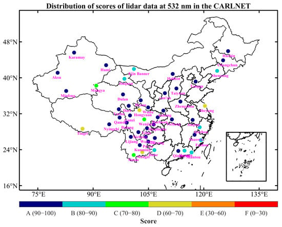
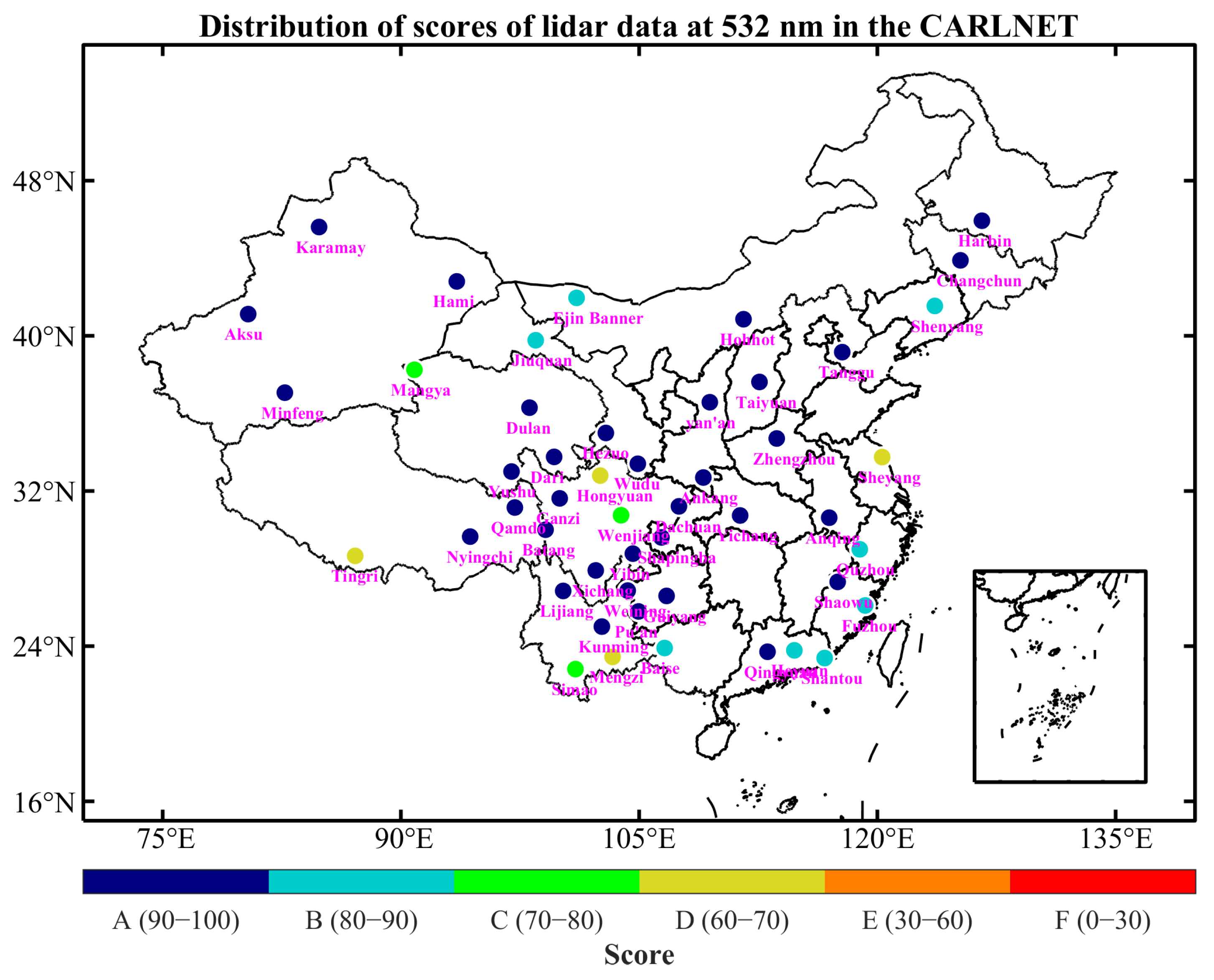
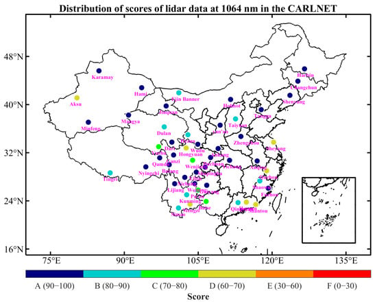
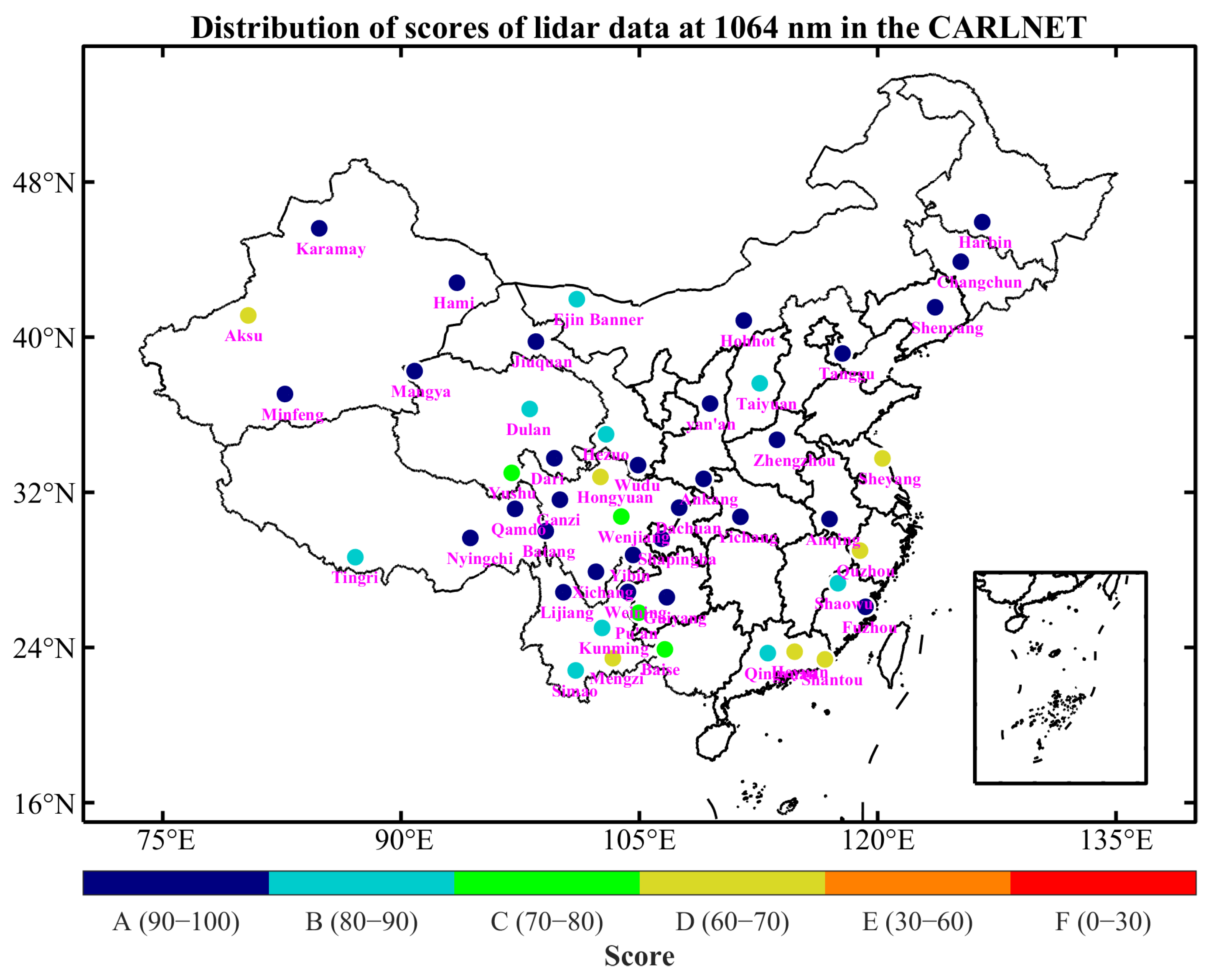
Currently, the raw-data quality assessment method proposed in this study has been applied to the CARLNET, which is capable of assessing raw data at 355 nm, 532 nm, and 1064 nm. In this study, the raw-data quality was categorized into six tiers based on raw-data scores. Data scoring 90–100 is labeled category A, indicating excellent quality; data scoring 80–90 is labelled category B, indicating good quality; data scoring 70–80 is labelled category C, indicating moderate quality; data scoring 60–70 is labelled category D, indicating mediocre quality; data scoring 30–60 is labelled category E, indicating quality issues; and data scoring 0–30 is labelled category F, indicating severe quality issues.
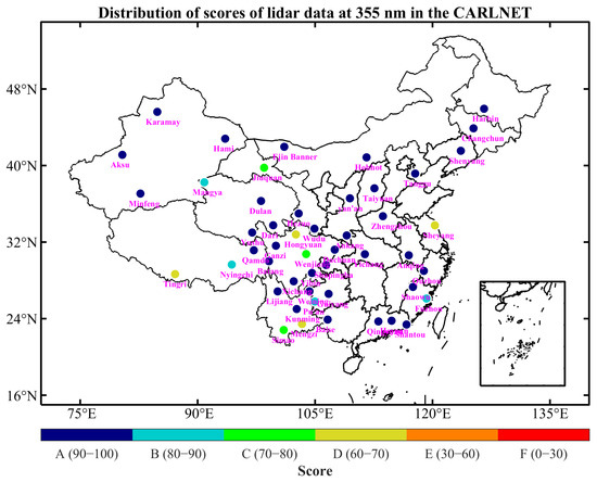
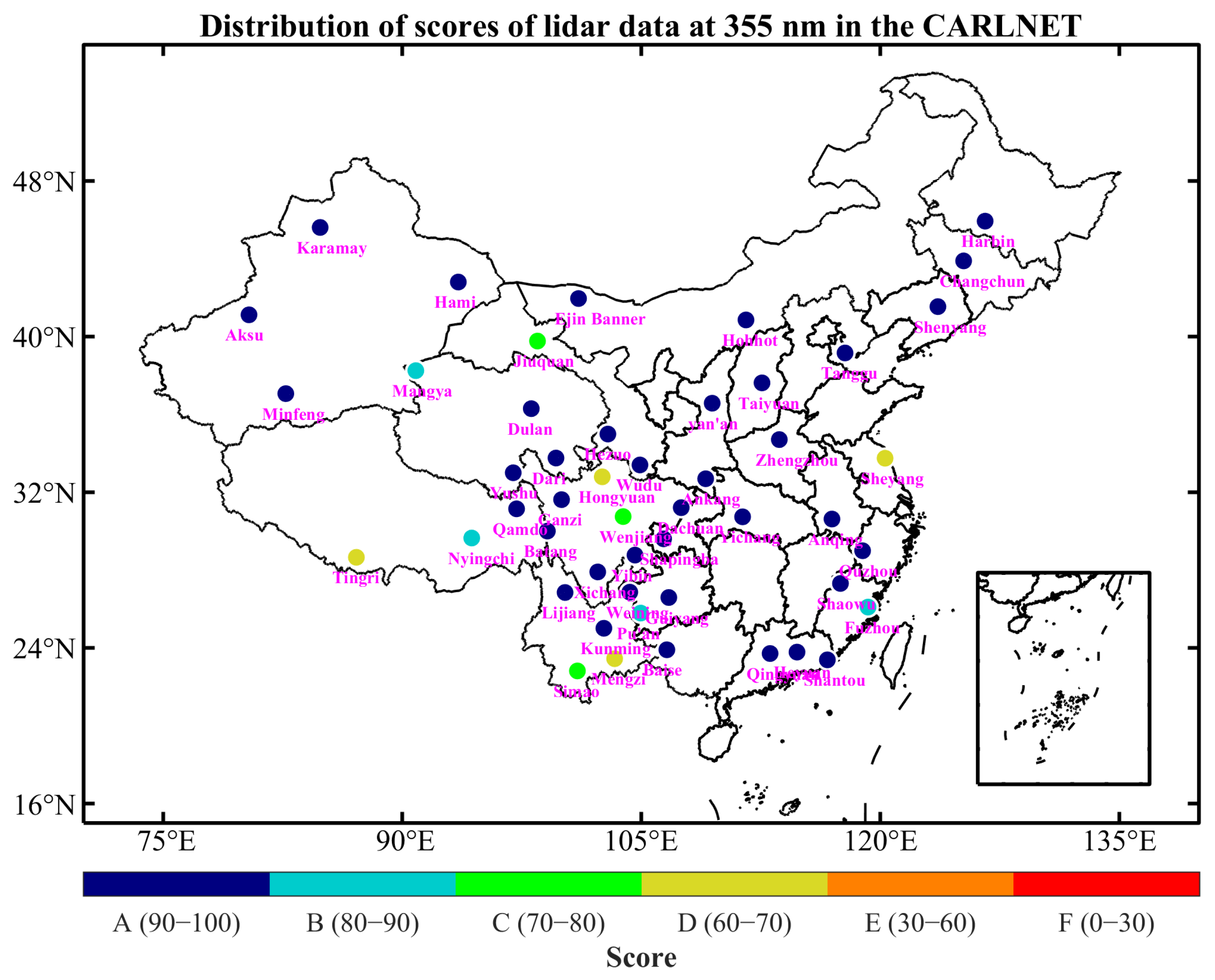
Figure 20, Figure 21 and Figure 22 show an example of the spatial distribution of lidar data scores at 355 nm, 532 nm and 1064 nm across 49 observation sites. The assessment time is 13 July 2025, at 15:00 UTC. As shown in the figure, lidar stations are widely distributed across diverse terrains, including plateaus, plains, hills, desert fringes, grasslands, and coastal areas. This extensive network provides crucial data support for studying national climate change, weather forecasting, and environmental protection.
Figure 20.
Distribution of the scores of lidar at 355 nm in the CARLNET. The dots represent lidar sites. The colors of each dot indicate the lidar raw-data quality grades.
Figure 21.
Distribution of the scores of lidar at 532 nm in the CARLNET. The dots represent lidar sites. The colors of each dot indicate the lidar raw data quality grades.
Figure 22.
Distribution of the scores of lidar at 1064 nm in the CARLNET. The dots represent lidar sites. The colors of each dot indicate the lidar raw-data quality grades.
As shown in Figure 20, Figure 21 and Figure 22, the scores of all observation sites were over 60. For data at 355 nm, the number of stations with data quality graded as A, B, C and D were 38 (78%), 4 (8%), 3 (6%) and 4 (8%) respectively; for data at 532 nm, the number of stations with data quality graded as A, B, C and D were 34 (70%), 8 (16%), 3 (6%) and 4 (8%) respectively; for data at 1064 nm, the number of stations with data quality graded as A, B, C and D were 29 (60%), 9 (18%), 4 (8%) and 7 (14%) respectively. Over 69% of observation sites achieved raw-data scores above 80 (Grade A and B) for all three wavelengths (355 nm, 532 nm and 1064 nm), which suggested that the lidar network has been constructed stably and the lidar raw-data quality was reliable.
During the observation period, the data scores from coastal observation sites were relatively lower than those from central and northern regions. Both the data at 355 nm and 532 nm at four stations were rated as grade D, and these stations are identical: Dingri, Hongyuan, Mengzi and Sheyang. The data scores for the wavelengths of 355 nm and 532 nm at the Wenjiang and Simao stations were both rated as grade C. This indicates good consistency between the data at 355 nm and 532 nm. Overall, the scores for 355 nm and 532 nm are higher than those for 1064 nm.
The examples demonstrate that the proposed lidar raw-data quality assessment method can distinguish the different data qualities. It can reflect the distribution and variation patterns of lidar network data quality, providing effective support for subsequent scientific research.
4. Discussion
The quality assessment method proposed in this study is primarily to assess the lidar raw-data quality of the CARLNET rapidly and in real time, and identify issues of lidar hardware with the scoring results. The results and analysis in Section 3 show that this quality assessment method can indeed achieve this purpose. Currently, this method has been applied to the CARLNET, and the lidar raw data is labeled. Data quality assessment provides crucial guidance for data applications such as data assimilation. For instance, when data assimilation requires the retrieval result profile to reach 3 km in height, data with Rayleigh fit scores exceeding 60 can be selected. This quality assessment method provides a feasible solution for assessing lidar raw-data quality and is also applicable to other aerosol lidar networks.
However, this method also has room for improvement. This study uses three factors (signal saturation at near-range, Rayleigh fit and effective detection range) to assess the lidar raw-data quality. Though this method can distinguish lidar raw-data quality under different scenarios, the differentiation lacks sufficient granularity. Therefore, raw-data quality is categorized into six grades based on the scoring results: A (90–100), B (80–90), C (70–80), D (60–70), E (30–60) and F (0–30). In addition, this study uses relatively simple methods (such as linear interpolation) to score the three assessment factors, and the used weight values are empirical rather than quantitative, where there is room for further optimization. Furthermore, the assessment results obtained through the proposed method can identify that issues exist with the lidar system, and infer what might cause the issue. However, it cannot currently determine the exact causes of the issues.
With the continuous upgrades to the CARLNET, it is expected to enable real-time transmission of both lidar hardware status parameters and weather condition parameters. This will enable additional assessment factors to be incorporated, thereby enhancing the precision and differentiation of quality assessment results. Additionally, the identification of causes for lidar issues will become more precise.
Furthermore, in future work, we will cross-compare the lidar raw-data assessment results by the proposed method with those obtained by manual quality control (QC), obtaining verification indicators such as accuracy and false-positive rate, thereby further enhancing the precision of quality assessment results.
Moreover, atmospheric lidar technology is undergoing profound integration with emerging computational and intelligent methodologies. Machine learning algorithms have broad application prospects. Constructing a large-scale, consistently annotated training dataset for the CARLNET that encompasses all fault modes, weather conditions, and site types is a crucial support for the effective application of machine learning in lidar. Our current work is laying an important data foundation and assessment benchmark for the future introduction and integration of machine learning methods.
5. Conclusions
The lidar raw data quality significantly impacts subsequent applications in meteorology and environmental protection. To address this issue, this study proposes and implements a comprehensive lidar raw-data quality assessment method tailored to China’s large-scale operationalized lidar network (CARLNET). Based on research methodology by MAO et al. [45], and considering the operational context of the CARLNET, this study selects three factors, signal saturation at near-range, Rayleigh fit, and effective detection range, to assess lidar raw data. By establishing scoring criteria, each of the three factors is evaluated separately, and then a weighted average is applied to derive the total score for the lidar raw data.
This study analyzes and discusses the proposed quality assessment method. We assessed the raw-data quality from three lidars under three different scenarios. The results show that the proposed method for assessing lidar raw signals can effectively distinguish lidar raw-data quality under different weather scenarios. In addition, the potential issues of lidar systems can be reflected to a certain extent by the proposed method. If the lidar data at a certain site shows a continuous or trending decline in assessment scores that cannot be attributed to weather conditions, there may be an issue with the lidar system. Moreover, if the assessment scores are significantly and continuously lower than those of other similar devices in the region under similar atmospheric conditions, this lidar is highly likely to have a system issue. Therefore, abnormal scores obtained by the proposed assessment method in this study can serve as an early warning for potential issues of lidar system. Through continuous anomaly scores for the effective detection range of the lidar, we identified two issues: optical-axis misalignment and signal-receiving issues. The results indicate that the proposed method can reveal certain hardware issues based on the results of raw-data quality assessment. We performed a statistical analysis of the raw-data quality of the CARLNET. Temporally, the scoring results from five representative stations over a one-year period were analyzed. The results showed that the scores could reflect seasonal variations and overall situation in data quality, and the consistency of raw-data quality across the three wavelengths is relatively good. Spatially, the scoring results from all 49 lidar stations across the CARLNET were analyzed. The results showed that over 69% of observation sites scored above 80 in raw data across all three wavelengths, indicating that the lidar network has been constructed stably and the lidar raw-data quality was reliable.
The method proposed in this study can provide support for subsequent scientific research in weather processes, aerosol transport, climate change, environmental protection, and other fields.
Author Contributions
Conceptualization, Z.B., X.W., Y.C. and P.Z.; methodology, S.M., Z.Y. and X.W.; validation, Z.B., Y.D., S.M. and Q.W.; formal analysis, S.M. and X.W.; investigation, Z.B., Y.D., S.M., Q.W., Z.Y. and Y.W.; resources, Y.C. and P.Z.; data curation, Y.D., S.M. and Y.W.; writing—original draft preparation, Z.B. and S.M.; writing—review and editing, Z.B., Y.D., S.M., Q.W., Z.Y., Y.C. and P.Z.; supervision, Y.C.; project administration, Z.B. and Y.D.; funding acquisition, Y.C. and P.Z. All authors have read and agreed to the published version of the manuscript.
Funding
This research was funded by the National Natural Science Foundation of China (U2442214), the National Key Research and Development Program of China (2023YFC3007800 and 2023YFC3007802), and the Scientific Research Project of Tianjin Meteorological Bureau (202525ybxm21).
Data Availability Statement
The original contributions presented in this study are included in the article. Further inquiries can be directed to the corresponding author.
Conflicts of Interest
The authors declare no conflicts of interest.
References
- Che, H.; Xia, X.; Zhao, H.; Li, L.; Gui, K.; Zheng, Y.; Song, J.; Qi, B.; Zhu, J.; Miao, Y.; et al. Aerosol optical and radiative properties and their environmental effects in China: A review. Earth-Sci. Rev. 2024, 248, 104634. [Google Scholar] [CrossRef] [Scilit]
- Hong, Y.; Di Girolamo, L. An Overview of Aerosol Properties in Clear and Cloudy Sky Based on CALIPSO Observations. Earth Space Sci. 2022, 9, e2022EA002287. [Google Scholar] [CrossRef] [Scilit]
- Jin, S.; Ma, Y.; Li, H.; Liu, B.; Fan, R.; Zhang, M.; Lopatin, A.; Dubovik, O.; Hu, X.; Gong, W.; et al. Characterizing Aerosol Optical Properties and Direct Radiative Effects From the Perspective of Components: A Synergy Retrieval Study Based on Sun Photometer and Lidar in Central China. Geophys. Res. Lett. 2025, 52, e2024GL113448. [Google Scholar] [CrossRef] [Scilit]
- Chang, Y.; Hu, Q.; Goloub, P.; Podvin, T.; Veselovskii, I.; Ducos, F.; Dubois, G.; Saito, M.; Lopatin, A.; Dubovik, O.; et al. Retrieval of microphysical properties of dust aerosols from extinction, backscattering and depolarization lidar measurements using various particle scattering models. Atmos. Chem. Phys. 2025, 25, 6787–6821. [Google Scholar] [CrossRef] [Scilit]
- Ansmann, A.; Baars, H.; Tesche, M.; Müller, D.; Althausen, D.; Engelmann, R.; Pauliquevis, T.; Artaxo, P. Dust and smoke transport from Africa to South America: Lidar profiling over Cape Verde and the Amazon rainforest. Geophys. Res. Lett. 2009, 36, L11802. [Google Scholar] [CrossRef] [Scilit]
- Groß, S.; Freudenthaler, V.; Schepanski, K.; Toledano, C.; Schäfler, A.; Ansmann, A.; Weinzierl, B. Optical properties of long-range transported Saharan dust over Barbados as measured by dual-wavelength depolarization Raman lidar measurements. Atmos. Chem. Phys. 2015, 15, 11067–11080. [Google Scholar] [CrossRef] [Scilit]
- Hofer, J.; Althausen, D.; Abdullaev, S.F.; Makhmudov, A.N.; Nazarov, B.I.; Schettler, G.; Engelmann, R.; Baars, H.; Fomba, K.W.; Müller, K.; et al. Long-term profiling of mineral dust and pollution aerosol with multiwavelength polarization Raman lidar at the Central Asian site of Dushanbe, Tajikistan: Case studies. Atmos. Chem. Phys. 2017, 17, 14559–14577. [Google Scholar] [CrossRef] [Scilit]
- Pan, Y.; Quan, J.; Ma, P.; Liao, Z.; Jia, X.; Dou, Y.; Cheng, Z.; Lei, L.; Wang, Y.; Zheng, M.; et al. Mineral dust scavenges anthropogenic aerosols in polluted environment. Atmos. Environ. 2023, 309, 119938. [Google Scholar] [CrossRef] [Scilit]
- Ansmann, A.; Wagner, F.; Müller, D.; Althausen, D.; Herber, A.; von Hoyningen-Huene, W.; Wandinger, U. European pollution outbreaks during ACE 2: Optical particle properties inferred from multiwavelength lidar and star-Sun photometry. J. Geophys. Res.-Atmos. 2002, 107, AAC-8. [Google Scholar] [CrossRef] [Scilit]
- Xian, J.; Sun, D.; Xu, W.; Han, Y.; Zheng, J.; Peng, J.; Yang, S. Urban air pollution monitoring using scanning Lidar. Environ. Pollut. 2020, 258, 113696. [Google Scholar] [CrossRef] [Scilit]
- Wong, M.S.; Qin, K.; Lian, H.; Campbell, J.R.; Lee, K.H.; Sheng, S. Continuous ground-based aerosol Lidar observation during seasonal pollution events at Wuxi, China. Atmos. Environ. 2017, 154, 189–199. [Google Scholar] [CrossRef] [Scilit]
- Lolli, S.; Sicard, M.; Amato, F.; Comeron, A.; Gíl-Diaz, C.; Landi, T.C.; Munoz-Porcar, C.; Oliveira, D.; Dios Otin, F.; Rocadenbosch, F.; et al. Climatological assessment of the vertically resolved optical and microphysical aerosol properties by lidar measurements, sun photometer, and in situ observations over 17 years at Universitat Politècnica de Catalunya (UPC) Barcelona. Atmos. Chem. Phys. 2023, 23, 12887–12906. [Google Scholar] [CrossRef] [Scilit]
- Heese, B.; Baars, H.; Bohlmann, S.; Althausen, D.; Deng, R. Continuous vertical aerosol profiling with a multi-wavelength Raman polarization lidar over the Pearl River Delta, China. Atmos. Chem. Phys. 2017, 17, 6679–6691. [Google Scholar] [CrossRef] [Scilit]
- Haarig, M.; Ansmann, A.; Engelmann, R.; Baars, H.; Toledano, C.; Torres, B.; Althausen, D.; Radenz, M.; Wandinger, U. First triple-wavelength lidar observations of depolarization and extinction-to-backscatter ratios of Saharan dust. Atmos. Chem. Phys. 2022, 22, 355–369. [Google Scholar] [CrossRef] [Scilit]
- Haarig, M.; Ansmann, A.; Baars, H.; Jimenez, C.; Veselovskii, I.; Engelmann, R.; Althausen, D. Depolarization and lidar ratios at 355, 532, and 1064 nm and microphysical properties of aged tropospheric and stratospheric Canadian wildfire smoke. Atmos. Chem. Phys. 2018, 18, 11847–11861. [Google Scholar] [CrossRef] [Scilit]
- Bohlmann, S.; Baars, H.; Radenz, M.; Engelmann, R.; Macke, A. Ship-borne aerosol profiling with lidar over the Atlantic Ocean: From pure marine conditions to complex dust–smoke mixtures. Atmos. Chem. Phys. 2018, 18, 9661–9679. [Google Scholar] [CrossRef] [Scilit]
- Redemann, J.; Gao, L. A machine learning paradigm for necessary observations to reduce uncertainties in aerosol climate forcing. Nat. Commun. 2024, 15, 8343. [Google Scholar] [CrossRef] [Scilit] [PubMed]
- Shin, J.; Sim, J.; Tesche, M.; Yoon, J.; Kim, D.; Noh, Y. Machine learning-based retrieval of aerosol size and hygroscopicity using horizontal scanning LiDAR and PM data. npj Clim. Atmos. Sci. 2025, 9, 3. [Google Scholar] [CrossRef] [Scilit]
- Ma, Y.; Zhu, Y.; Liu, B.; Li, H.; Jin, S.; Zhang, Y.; Fan, R.; Gong, W. Estimation of the vertical distribution of particle matter (PM2.5) concentration and its transport flux from lidar measurements based on machine learning algorithms. Atmos. Chem. Phys. 2021, 21, 17003–17016. [Google Scholar] [CrossRef] [Scilit]
- del Águila, A.; Ortiz-Amezcua, P.; Tabik, S.; Bravo-Aranda, J.A.; Fernández-Carvelo, S.; Alados-Arboledas, L. Aerosol type classification with machine learning techniques applied to multiwavelength lidar data from EARLINET. Atmos. Chem. Phys. 2025, 25, 12549–12567. [Google Scholar] [CrossRef] [Scilit]
- Ferrare, R.; Hair, J.; Shingler, T.; Hostetler, C.; Nehrir, A.; Fenn, M.; Scarino, A.J.; Burton, S.; Clayton, M.; Collins, J.; et al. Particulate matter concentrations derived from airborne high spectral resolution lidar measurements using machine learning regression. Atmos. Meas. Tech. 2025, 18, 7735–7766. [Google Scholar] [CrossRef] [Scilit]
- Lewis, J.R.; Campbell, J.R.; Welton, E.J.; Stewart, S.A.; Haftings, P.C. Overview of MPLNET Version 3 Cloud Detection. J. Atmos. Ocean. Technol. 2016, 33, 2113–2134. [Google Scholar] [CrossRef] [Scilit]
- Lewis, J.R.; Welton, E.J.; Molod, A.M.; Joseph, E. Improved boundary layer depth retrievals from MPLNET. J. Geophys. Res.-Atmos. 2013, 118, 9870–9879. [Google Scholar] [CrossRef] [Scilit]
- Gross, B.; Lewis, J.R.; Welton, E.J.; Campbell, J.R.; Haftings, P.C.; Moshary, F.; Arend, M. MPLNET V3 Cloud and Planetary Boundary Layer Detection. EPJ Web Conf. 2016, 119, 16011. [Google Scholar] [CrossRef] [Scilit]
- Welton, E.J.; Stewart, S.A.; Lewis, J.R.; Belcher, L.R.; Campbell, J.R.; Lolli, S. Status of the NASA Micro Pulse Lidar Network (MPLNET): Overview of the Network and Future Plans, New Version 3 Data Products, and the Polarized MPL. In Proceedings of the 28th International Laser Radar Conference, Bucharest, Romania, 25–30 June 2018; Volume 176, p. 09003. [Google Scholar] [CrossRef] [Scilit]
- Pappalardo, G.; Amodeo, A.; Apituley, A.; Comeron, A.; Freudenthaler, V.; Linné, H.; Ansmann, A.; Bösenberg, J.; D’Amico, G.; Mattis, I.; et al. EARLINET: Towards an advanced sustainable European aerosol lidar network. Atmos. Meas. Tech. 2014, 7, 2389–2409. [Google Scholar] [CrossRef] [Scilit]
- Kokkalis, P. Using paraxial approximation to describe the optical setup of a typical EARLINET lidar system. Atmos. Meas. Tech. 2017, 10, 3103–3115. [Google Scholar] [CrossRef] [Scilit]
- Mylonaki, M.; Giannakaki, E.; Papayannis, A.; Papanikolaou, C.-A.; Komppula, M.; Nicolae, D.; Papagiannopoulos, N.; Amodeo, A.; Baars, H.; Soupiona, O. Aerosol type classification analysis using EARLINET multiwavelength and depolarization lidar observations. Atmos. Chem. Phys. 2021, 21, 2211–2227. [Google Scholar] [CrossRef] [Scilit]
- Sicard, M.; D’Amico, G.; Comerón, A.; Mona, L.; Alados-Arboledas, L.; Amodeo, A.; Baars, H.; Baldasano, J.M.; Belegante, L.; Binietoglou, I.; et al. EARLINET: Potential operationality of a research network. Atmos. Meas. Tech. 2015, 8, 4587–4613. [Google Scholar] [CrossRef] [Scilit]
- Althausen, D.; Engelmann, R.; Baars, H.; Heese, B.; Ansmann, A.; Müller, D.; Komppula, M. Portable Raman Lidar PollyXT for Automated Profiling of Aerosol Backscatter, Extinction, and Depolarization. J. Atmos. Ocean. Technol. 2009, 26, 2366–2378. [Google Scholar] [CrossRef] [Scilit]
- Engelmann, R.; Kanitz, T.; Baars, H.; Heese, B.; Althausen, D.; Skupin, A.; Wandinger, U.; Komppula, M.; Stachlewska, I.S.; Amiridis, V.; et al. The automated multiwavelength Raman polarization and water-vapor lidar Polly XT: The neXT generation. Atmos. Meas. Tech. 2016, 9, 1767–1784. [Google Scholar] [CrossRef] [Scilit]
- Baars, H.; Kanitz, T.; Engelmann, R.; Althausen, D.; Heese, B.; Komppula, M.; Preißler, J.; Tesche, M.; Ansmann, A.; Wandinger, U.; et al. An overview of the first decade of PollyNET: An emerging network of automated Raman-polarization lidars for continuous aerosol profiling. Atmos. Chem. Phys. 2016, 16, 5111–5137. [Google Scholar] [CrossRef] [Scilit]
- Nicolae, D.; Sugimoto, N.; Shimizu, A.; Nishizawa, T.; Jin, Y.; Makoto, A.; Vassilis, A.; Balis, D.; Behrendt, A.; Comeron, A.; et al. Recent developments with the asian dust and aerosol lidar observation network (AD-NET). EPJ Web Conf. 2018, 176, 09001. [Google Scholar] [CrossRef] [Scilit]
- Gross, B.; Nishizawa, T.; Sugimoto, N.; Matsui, I.; Shimizu, A.; Higurashi, A.; Jin, Y.; Moshary, F.; Arend, M. The Asian Dust and Aerosol Lidar Observation Network (AD-NET): Strategy and Progress. EPJ Web Conf. 2016, 119, 19001. [Google Scholar] [CrossRef] [Scilit]
- Huang, Z.; Huang, J.; Bi, J.; Wang, T.; Zhou, T.; Dong, Q.; Shi, J.; Liu, Q.; Li, W.; Li, Z.; et al. Dust observation by a ground-based lidar network along the global dust belt. E3S Web Conf. 2024, 575, 02006. [Google Scholar] [CrossRef] [Scilit]
- Liu, Q.; Huang, Z.; Liu, J.; Chen, W.; Dong, Q.; Wu, S.; Dai, G.; Li, M.; Li, W.; Li, Z.; et al. Validation of initial observation from the first spaceborne high-spectral-resolution lidar with a ground-based lidar network. Atmos. Meas. Tech. 2024, 17, 1403–1417. [Google Scholar] [CrossRef] [Scilit]
- Shao, N.; Wang, Q.; Bu, Z.; Yin, Z.; Dai, Y.; Chen, Y.; Wang, X. China Aerosol Raman Lidar Network (CARLNET)—Part I: Water Vapor Raman Channel Calibration and Quality Control. Remote Sens. 2025, 17, 414. [Google Scholar] [CrossRef] [Scilit]
- Talagrand, O. Assimilation of Observations, an Introduction (gtSpecial IssueltData Assimilation in Meteology and Oceanography: Theory and Practice). J. Meteorol. Soc. Jpn. 1997, 75, 191–209. [Google Scholar] [CrossRef] [Scilit]
- Freudenthaler, V.; Linné, H.; Chaikovski, A.; Rabus, D.; Groß, S. EARLINET lidar quality assurance tools. Atmos. Meas. Tech. Discuss. 2018, 1–35. [Google Scholar] [CrossRef] [Scilit]
- Gross, B.; Pappalardo, G.; Freudenthaler, V.; Nicolae, D.; Mona, L.; Belegante, L.; D’Amico, G.; Moshary, F.; Arend, M. Lidar Calibration Centre. EPJ Web Conf. 2016, 119, 19003. [Google Scholar] [CrossRef] [Scilit]
- Bockmann, C.; Wandinger, U.; Ansmann, A.; Bosenberg, J.; Amiridis, V.; Boselli, A.; Delaval, A.; De Tomasi, F.; Frioud, M.; Grigorov, I.V.; et al. Aerosol lidar intercomparison in the framework of the EARLINET project. 2. Aerosol backscatter algorithms. Appl. Opt. 2004, 43, 977–989. [Google Scholar] [CrossRef] [Scilit]
- D’Amico, G.; Amodeo, A.; Baars, H.; Binietoglou, I.; Freudenthaler, V.; Mattis, I.; Wandinger, U.; Pappalardo, G. EARLINET Single Calculus Chain—Overview on methodology and strategy. Atmos. Meas. Tech. 2015, 8, 4891–4916. [Google Scholar] [CrossRef] [Scilit]
- D’Amico, G.; Amodeo, A.; Mattis, I.; Freudenthaler, V.; Pappalardo, G. EARLINET Single Calculus Chain—Technical—Part 1: Pre-processing of raw lidar data. Atmos. Meas. Tech. 2016, 9, 491–507. [Google Scholar] [CrossRef] [Scilit]
- Mattis, I.; D’Amico, G.; Baars, H.; Amodeo, A.; Madonna, F.; Iarlori, M. EARLINET Single Calculus Chain—Technical—Part 2: Calculation of optical products. Atmos. Meas. Tech. 2016, 9, 3009–3029. [Google Scholar] [CrossRef] [Scilit]
- Mao, S.; Yin, Z.; Wang, L.; Wei, Y.; Bu, Z.; Chen, Y.; Dai, Y.; Müller, D.; Wang, X. Aerosol Optical Properties Retrieved by Polarization Raman Lidar: Methodology and Strategy of a Quality-Assurance Tool. Remote Sens. 2024, 16, 207. [Google Scholar] [CrossRef] [Scilit]
- Qiu, J.; Zong, X.; Zhang, X. A study of the scaling height of the tropospheric aerosol and its extinction coefficient profile. J. Aerosol. Sci. 2005, 36, 361–371. [Google Scholar] [CrossRef] [Scilit]

Disclaimer/Publisher’s Note: The statements, opinions and data contained in all publications are solely those of the individual author(s) and contributor(s) and not of MDPI and/or the editor(s). MDPI and/or the editor(s) disclaim responsibility for any injury to people or property resulting from any ideas, methods, instructions or products referred to in the content. |
© 2026 by the authors. Licensee MDPI, Basel, Switzerland. This article is an open access article distributed under the terms and conditions of the Creative Commons Attribution (CC BY) license.