


Highlights
What are the main findings?
- A CNN pre-trained on RGB images, combined with a 15-to-3 channel feature-encoding branch, can effectively classify seven salt marsh vegetation classes from multispectral UAV data.
- The deep learning model significantly outperforms traditional machine learning classifiers (Support Vector Machines and Random Forest), achieving an overall accuracy of 98.4% when using spectral bands and vegetation indices together.
What is the implication of the main findings?
- The proposed framework enables accurate, high-resolution mapping of heterogeneous salt marsh vegetation, supporting ecological monitoring and management.
- Integrating UAV-based multispectral imagery with pre-trained CNNs provides a transferable methodology for other multispectral vegetation classification tasks, reducing the need for extensive training datasets.
Abstract
Accurate classification of salt marsh vegetation is crucial for coastal wetland monitoring, but fine-grained species discrimination remains difficult, particularly when only limited training data are available for deep learning approaches. To address this challenge, this paper presents a transfer learning-based framework for classifying salt marsh vegetation using UAV multispectral imagery, focusing on a seven-class taxonomy representative of dominant species and water surfaces. Multispectral orthophotos acquired with a MicaSense Dual-Camera system (10 spectral bands) are combined with five vegetation indices to create rich multi-channel inputs. A classification architecture inspired by heterogeneous transfer learning is developed, where a feature-encoding branch compresses the 15-channel input into three channels before processing through a VGG-16 Convolutional Neural Network (CNN), pre-trained on RGB imagery. By leveraging transfer learning from VGG-16, the proposed model achieves high classification accuracy even with limited training data. Performance is compared with traditional machine learning classifiers, namely Support Vector Machines (SVMs) and Random Forest (RF). Results show that the deep learning approach significantly outperforms SVM and RF, achieving an overall accuracy of 98.4% when jointly using spectral bands and vegetation indices. These findings demonstrate the potential of integrating multispectral UAV data and CNN-based classification to support accurate mapping of heterogeneous salt marsh communities for ecological monitoring and coastal management.
1. Introduction
Coastal lagoons are waterbodies partially separated from the sea by sedimentary barriers [1,2], covering approximately 13% of coastlines worldwide and forming transitional zones between terrestrial, marine, and freshwater environments [3]. Rich in biodiversity, these ecosystems act as essential buffers between land and sea, shaped by freshwater inputs from river deltas and periodic tidal currents, which generate strong physical gradients and frequent environmental disturbances [4,5,6,7,8,9]. However, the interaction between natural processes and human activities, together with the sensitivity of these systems to global environmental change, has made coastal lagoons among the most threatened ecosystems globally [10,11,12,13,14,15,16]. Salt marshes constitute a primary habitat within lagoons and are closely linked to the environmental dynamics of these systems. They consist of sedimentary bodies composed of fine materials transported and mixed by currents, stabilized by halophilous vegetation [17]. Tidal submergence is a key factor in the formation and maintenance of salt marshes, regulating the ecology of the entire environment by determining nutrient supply, sediment deposition, and by influencing species distribution [18,19]. The vegetation in salt marshes shows relatively low species diversity but is rich in endemisms [20], and exhibits strong zonation driven by seawater inundation, with species distributed according to their tolerance to waterlogging stress [21].
In this context, the classification of salt marsh environments provides a clear picture of species distribution and enables monitoring of changes in submergence gradients over time. Traditional in situ mapping of salt marsh vegetation is often labor-intensive, time-consuming, and limited in spatial coverage, making it difficult to capture the full heterogeneity of these ecosystems. In contrast, remote sensing has become an increasingly valuable tool, enabling spatially extensive, repeatable, and cost-effective observations of ecosystem dynamics [22]. The emergence of Uncrewed Aerial Vehicles (UAVs) has further enhanced ecological monitoring by providing high-resolution data acquisition with flexible revisit times [23].
Among remote sensing technologies, multispectral imaging has proven particularly effective for ecological applications. Unlike conventional RGB cameras, multispectral and hyperspectral sensors capture surface reflectance across multiple narrow wavelength bands, enabling the detection of vegetation properties that are not discernible through conventional visible spectrum imaging alone. In the context of UAV-based surveys, multispectral imagery offers a valuable combination of high spatial resolution and enhanced spectral information, making it well suited for capturing the fine spatial heterogeneity typical of salt marsh vegetation [24,25]. Moreover, recent studies demonstrate that incorporating vegetation indices (VIs) into the classification pipeline can substantially improve salt marsh species identification [26,27,28]. Indices such as the Normalized Difference Vegetation Index (NDVI) [29], Green Normalized Difference Vegetation Index (GNDVI) [30], and Modified Soil Adjusted Vegetation Index (MSAVI) [31], which can be easily derived from multispectral imagery, provide a compact and interpretable representation of spectral responses related to plant health, biomass, and chlorophyll content, and can be directly fed into classification algorithms [32]. However, despite the spectral richness provided by multispectral bands and vegetation indices, salt marsh vegetation often remains difficult to discriminate at the species level, as fine-grained zonation patterns and spatial mosaics are characterized by partially overlapping spectral responses, posing significant challenges for accurate classification.
Coupled with the increasing availability of high-resolution multispectral data, a wide range of supervised classification approaches has been applied to salt marsh vegetation mapping. Traditional pixel-based classifiers, such as Spectral Angle Mapper and Maximum Likelihood methods, have been used in several studies [33,34], but their performance often degrades when vegetation classes exhibit overlapping spectral signatures. To overcome these limitations, Machine Learning (ML) algorithms have gained prominence in salt marsh applications. In particular, Support Vector Machines (SVM) and Random Forest (RF) classifiers have proven effective in handling high-dimensional multispectral inputs and integrating spectral bands, vegetation indices, and additional features [35,36]. For example, RF-based approaches applied to UAV multispectral imagery have achieved overall accuracies of up to 96.8% in salt marsh environments when combining spectral information and texture features [37], while cascaded workflows integrating unsupervised clustering, Spectral Angle Mapper, and SVM have reported accuracies approaching 98% [38]. Other studies have explored gradient-boosting methods, such as XGBoost, particularly for satellite-based time-series classification, achieving overall accuracies around 81% for multi-class salt marsh mapping [39]. Despite these promising results, ML approaches typically rely on hand-crafted features and operate either at the pixel level or on spatially aggregated representations, which limits their ability to fully exploit spatial context and to model the hierarchical spatial–spectral patterns characteristic of salt marsh vegetation. This constraint becomes particularly critical in highly heterogeneous environments, where strong zonation, subtle inter-species differences, and pronounced class imbalance are common. These challenges have motivated the adoption of Deep Learning (DL) approaches, which move beyond feature engineering by learning task-driven representations directly from image data.
Building on the limitations of traditional ML approaches, deep learning methods based on convolutional neural networks (CNNs) have therefore been increasingly applied to coastal vegetation classification, with several studies demonstrating the potential of DL approaches in salt marsh environments [40]. For instance, a DL model has achieved an overall accuracy of 94.6% for multi-class vegetation classification, outperforming conventional pixel- and object-based ML methods [41]. Similarly, UAV-based multispectral imagery analyzed with encoder–decoder architectures, including U-Net and SegNet, has reported overall accuracies of 94.1% and 93.3%, respectively, compared to values below 85% obtained with RF and gradient-boosting classifiers [42]. These results highlight the ability of DL models to exploit both spectral information and spatial context, leading to improved class separability in complex and heterogeneous salt marsh landscapes. However, the widespread adoption of deep learning for salt marsh vegetation classification is still restricted by practical constraints, primarily related to the availability of large, manually annotated training datasets. In salt marsh environments, the acquisition of extensive ground-truth data is often hindered by the time-consuming nature of field surveys and the spatial fragmentation of vegetation patches. As a consequence, training deep neural networks from scratch is frequently impractical and may lead to overfitting or limited generalization when only small annotated datasets are available.
To address these constraints, this work proposes a transfer learning–based framework that explicitly adapts an RGB-pretrained CNN to multispectral UAV imagery for fine-grained salt marsh vegetation classification. In the literature, transfer learning has been widely adopted to leverage CNNs pre-trained on large image datasets, enabling effective feature reuse when training data are scarce [43]. However, the direct transfer of RGB-pretrained CNNs to multispectral imagery is non-trivial due to differences in spectral dimensionality, sensor characteristics, and data distributions, which require dedicated adaptation strategies. Heterogeneous transfer learning approaches have been proposed to address this challenge, particularly in hyperspectral image classification. For example, ref. [44] demonstrated that mapping hyperspectral data into a feature space compatible with RGB-pretrained CNNs can significantly improve classification performance under limited training data conditions. Related strategies have also been explored in multispectral remote sensing applications, including UAV-based vegetation classification, where transfer learning schemes have shown improved performance for mangrove community mapping [45]. Similarly, a two-stage transfer learning paradigm combining RGB-pretrained and multispectral feature representations has yielded consistent gains on airborne multispectral datasets [46]. More generally, recent researches have confirmed the effectiveness of DL and transfer learning strategies for multispectral and hyperspectral remote sensing data [47].
Despite these advances, the application of heterogeneous transfer learning to multispectral UAV imagery for fine-grained salt marsh vegetation classification remains relatively underexplored. The core idea of this work is to leverage a deep neural network pre-trained on a large RGB dataset and adapt it to multispectral inputs through a dedicated spectral–spatial mapping module. Trained on a limited number of annotated multispectral samples, this module transforms spectral bands and vegetation indices into three informative channels, enabling seamless integration with the pre-trained RGB backbone. By doing so, the approach retains the representational power and generalization capability of a large model, while avoiding the need to train a full CNN from scratch. As a result, the proposed method offers an effective and data-efficient solution for high-resolution salt marsh vegetation classification, suitable even in contexts where annotated multispectral datasets are scarce.
The remainder of this paper is organized as follows. Section 2 describes the study area, the data acquisition process, and the proposed multispectral classification framework, while Section 3 presents the experimental results. Section 4 discusses the performance and implications of the proposed approach in the context of salt marsh monitoring and outlines potential directions for future research. Finally, Section 5 summarizes the main conclusions of the study.
2. Materials and Methods
2.1. Study Area and Ground-Truth Field Data
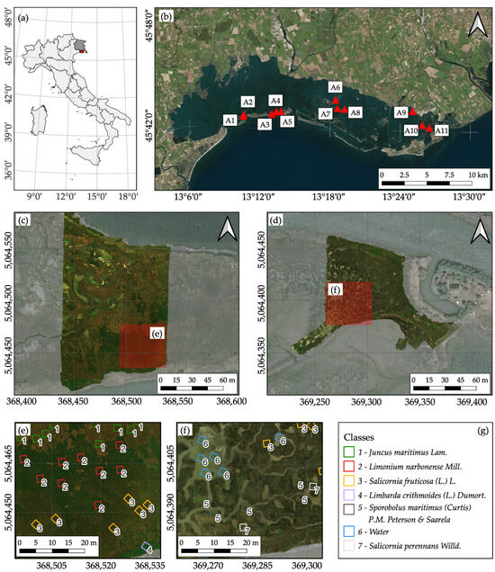
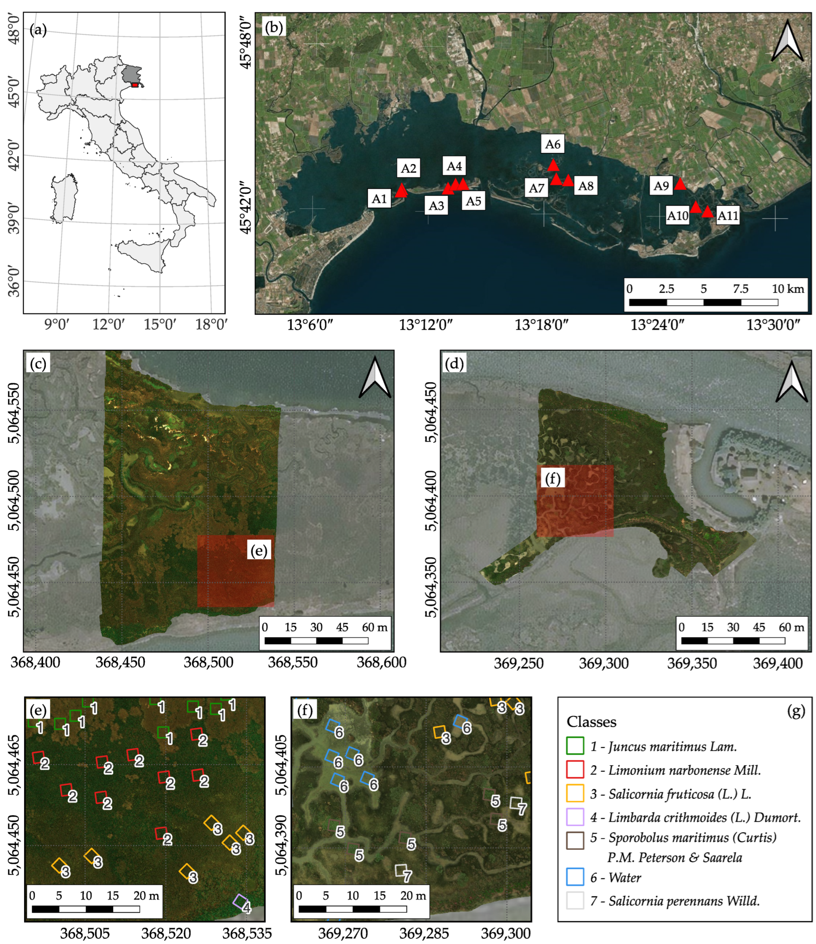
The study area is located within the Grado Lagoon (extending approximately from 45°42′10.5″N, 13°09′17.8″E to 45°40′49.8″N, 13°21′31.2″E) along the northern Adriatic coast in Friuli Venezia Giulia Region, Italy (Figure 1a,b). This coastal wetland is part of the Natura 2000 network and is designated both as a Special Area of Conservation and a Special Protection Area under site code IT3320037. The regional climate is characterized by mean annual precipitation of about 974 mm and marked seasonal temperature variability, with monthly averages ranging from roughly 3 °C in winter to nearly 29° in midsummer. From a geomorphological standpoint, the system is classified as a leaky lagoon, reflecting its combination of limited exchange with the open sea and strong internal compartmentalization. Tidal dynamics exert a dominant control: the lagoon experiences semi-diurnal tides with an average range of 0.65 m, reaching approximately 1.05 m during spring tides and decreasing to around 0.22 m during neap conditions [21,48]. More specifically, this study focuses on 11 selected sites within the lagoon (Figure 1b), spanning a total area of approximately 12 ha.
Figure 1.
(a) Location of the study area (red rectangle) within the Friuli Venezia Giulia Region, Italy. (b) Location of the 11 study sites in the Grado Lagoon. (c,d) RGB visualizations of the multispectral orthomosaics for areas A7 and A8. (e,f) Ground-truth field sampling plots, color-coded according to the class legend in (g), shown for the subareas highlighted in red in (c,d). Geographic coordinates are used in (a,b), while metric coordinates in the RDN2008/UTM Zone 33N reference system (EPSG:6708) are used in (c–f). Satellite basemaps are provided by Bing Maps.
Field data collection, which provided the ground truth for the classification framework, targeted six characteristic salt marsh species [49]—Juncus maritimus Lam., Limonium narbonense Mill., Salicornia fruticosa (L.) L., Limbarda crithmoides (L.) Dumort., Sporobolus maritimus (Curtis) P.M. Peterson & Saarela, and Salicornia perennans Willd.—and was carried out during the summer of 2023. A total of 421 monospecific plots, each measuring 2 m × 2 m, were delineated and georeferenced using a Global Navigation Satellite System (GNSS) receiver (Figure 1e,f). To provide a complete representation of the land-cover types relevant to multispectral classification, an additional set of 181 plots containing water was included as ground-truth reference. These samples exhibit substantial heterogeneity in depth, turbidity, and substrate visibility, capturing the typical variability of shallow lagoonal waters. In total, 602 plots were collected in situ, with the number of observations available for each class reported in Table 1. It is worth noting that the dataset presents a marked class imbalance, which mirrors the natural, spatially uneven distribution of species across the study areas.
Table 1.
Number of ground-truth plots available for each class. The plant nomenclature followed the Italian checklist [49].
2.2. UAV Acquisition Timing and Phenological Context
The multispectral UAV survey of the 11 study sites was conducted over four separate days in August 2023 under low-tide conditions within a semidiurnal tidal cycle, between neap and spring tide phases. This timing was intentionally selected to minimize the influence of tidal submergence on vegetation spectral signatures, while maximizing the exposure of low-marsh areas. In particular, dominant low-marsh species such as Sporobolus maritimus and Salicornia perennans were fully exposed during data acquisition, whereas tidal channels and intertidal flats remained partially inundated, allowing their inclusion as water-related surfaces in the resulting images. This acquisition strategy ensured consistent observation conditions across sites while preserving the representation of both vegetated and aquatic classes.
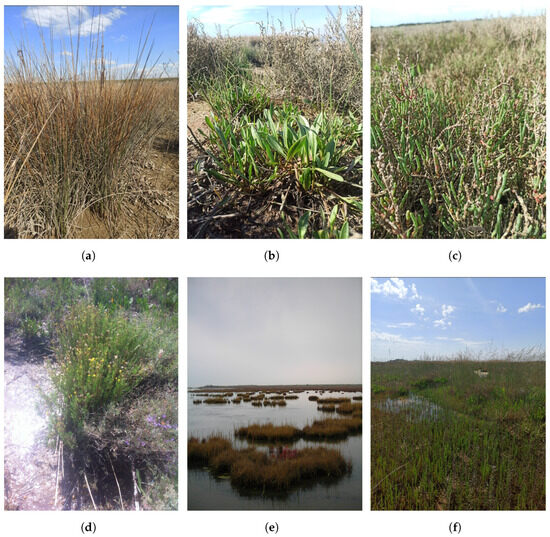
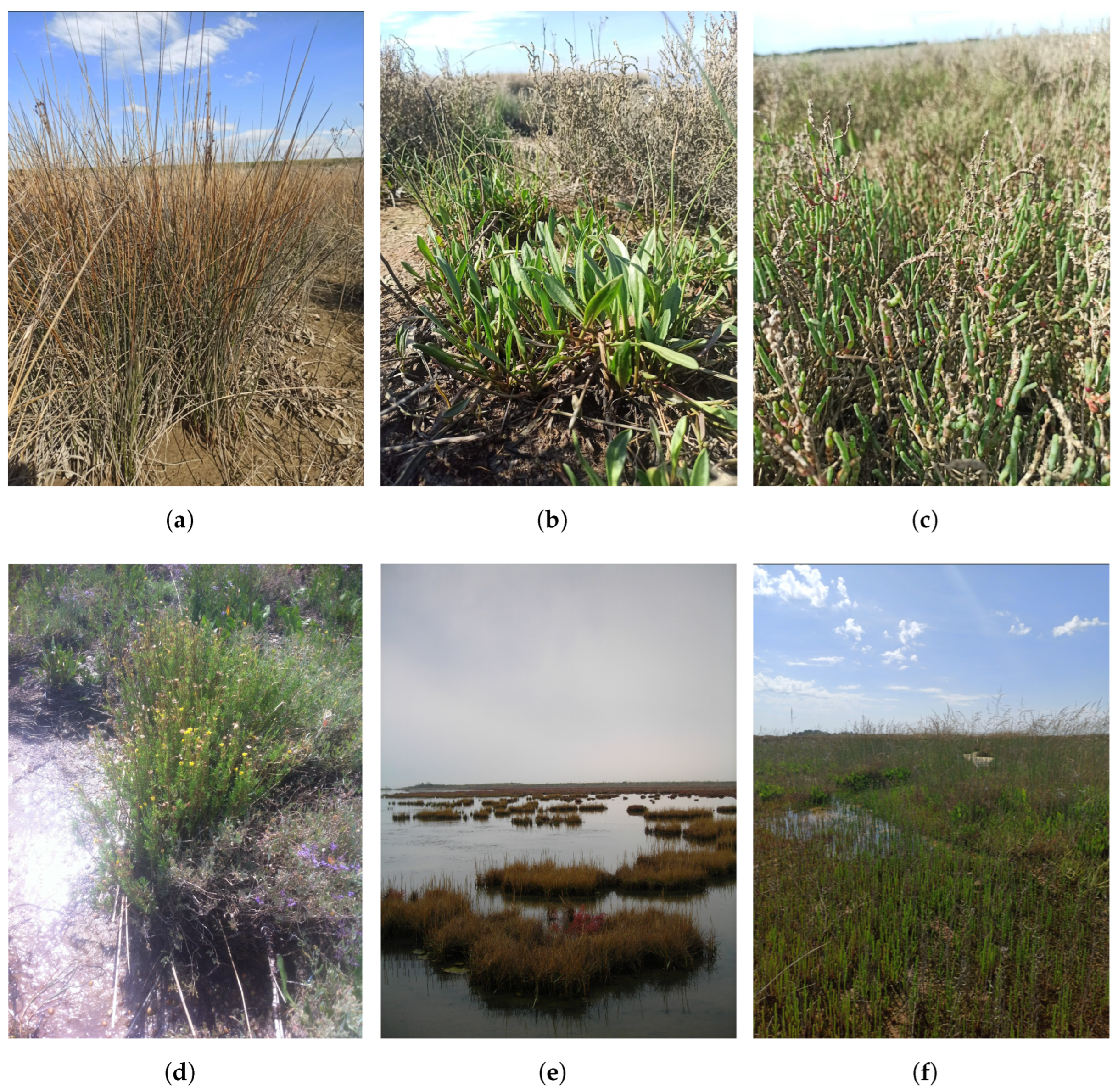
At the time of the survey, all target species were in an advanced vegetative stage with maximum canopy development. This phenological phase was selected to maximize interspecific phenological and structural contrasts among co-occurring species within the same environmental zones. Indeed, as shown in Figure 2, the considered species differ markedly in growth form, canopy structure, and spatial arrangement, which translates into distinctive textural and spectral patterns in high–spatial resolution multispectral UAV imagery. For example, Juncus maritimus forms dense, vertically structured canopies characterized by dark-green foliage and high standing biomass, resulting from continuous leaf turnover, which translates into strong near-infrared reflectance and homogeneous texture. In contrast, succulent species such as Salicornia spp. and Limbarda crithmoides are characterized by lower stature, articulated or fleshy tissues, and more heterogeneous spectral responses in the visible wavelength regions [50]. However, distinguishing between species belonging to the same genus (e.g., Salicornia fruticosa and Salicornia perennans), which mainly differ in architecture branching, still represents a challenge for image-based classification approaches. In addition to morphological variability, species-specific adaptations to salinity and inundation stress lead to a well-defined zonation across the salt marsh, with different communities occupying characteristic elevation ranges [51].
Figure 2.
Representative ground photos illustrating the morphological characteristics of the target salt marsh vegetation classes. (a) Juncus maritimus Lam. (b) Limonium narbonense Mill. (c) Salicornia fruticosa (L.) L. (d) Limbarda crithmoides (L.) Dumort. (e) Sporobolus maritimus (Curtis) P.M. Peterson & Saarela. (f) Salicornia perennans Willd.
The combination of morphological contrast and spatial organization provides a favorable context for UAV-based halophytic vegetation classification, while simultaneously highlighting the intrinsic challenges associated with fine-grained species discrimination from multispectral imagery acquired at a single time point. These acquisition conditions define the observational context of the multispectral dataset described in the following section.
2.3. Multispectral Sensor Configuration and Image Processing
Multispectral data acquisition was performed using a MicaSense Dual-Camera System (MicaSense Inc., Seattle, WA, USA) mounted on a DJI Matrice 210 v2 UAV (DJI, Nanshan, Shenzhen, China). The system combines a MicaSense RedEdge-MX and a RedEdge-MX Blue sensor, enabling the synchronized acquisition of 10 multispectral bands at a spatial resolution of 1280 × 960 pixels (Table 2). This configuration provides radiometrically stable measurements across a broad spectral range, making it suitable for diverse environmental applications—from shallow-water analysis using the coastal blue () aerosol band to vegetation monitoring based on green (), red (), red-edge (), and near-infrared () bands.
Table 2.
Spectral characteristics of the bands acquired by the MicaSense Dual-Camera system. The table reports, for each band, the central wavelength () and the Full Width at Half Maximum (FWHM), both expressed in nanometers.
UAV flights were conducted under varying illumination conditions. To mitigate radiometric variability, all images were calibrated using reflectance panel measurements acquired before and after each flight to establish an absolute radiometric reference. In addition, the multispectral system was equipped with a Downwelling Light Sensor (DLS), which continuously recorded incident sunlight and was used to compensate for variations in illumination intensity and geometry along the flight path. Radiometric calibration was performed using the standard workflow implemented in Agisoft Metashape Professional (version 2.0.4; Agisoft LLC, St. Petersburg, Russia).
Each study site was mapped through an independent UAV flight, ensuring a minimum image overlap of 80% in both forward and side directions to guarantee robust multi-view geometry. Image processing was carried out in Agisoft Metashape Professional (v. 2.0.4) using the photogrammetric pipeline adapted for multispectral imaging. In this workflow, one band is designated as the master image for tie-point extraction and bundle adjustment, while the remaining bands have fixed but unknown relative orientations with respect to the master one, to be estimated in the Structure-from-Motion phase. This approach preserves the rigidity among bands and ensures accurate alignment of the full multispectral stack. Dense point cloud generation and subsequent orthorectification resulted in a 10-band orthomosaic (Figure 1c,d) with a ground sampling distance (GSD) of 3 cm/pixel.
The original 10 spectral bands were augmented with 5 VIs, namely the Normalized Difference Vegetation Index (NDVI) [29], Normalized Difference Red Edge Index (NDRE) [52], Normalized Difference Water Index (NDWI) [53], Enhanced Vegetation Index (EVI) [54], and Modified Soil Adjusted Vegetation Index (MSAVI) [31]. These indices were selected based on their established ability to highlight specific vegetation properties relevant for salt marsh species identification (vegetation vigor, chlorophyll content, red-edge variation, and greenness), and follow the set of key indices for vegetation discrimination reported in [55]. NDRE, not included in that study, was additionally considered to explicitly exploit red-edge information in a vegetation index, which has proven effective for discriminating salt marsh vegetation [37]. The indices are defined by the following expressions:
For the computation of the VIs, the 10 spectral bands were reduced to 5 (B, G, R, , NIR) by averaging those corresponding to the same spectral region, but measured at slightly different wavelengths. It should be noted that all 10 original spectral bands provided by the MicaSense Dual-Camera System were retained and directly used as input features for the deep learning model, while band averaging was applied exclusively for VI computation. This choice follows a common practice in remote sensing, as most widely used vegetation indices are defined in terms of broad spectral regions rather than sensor-specific narrow bands. Averaging bands within the same spectral region allows VIs to remain consistent with their original biophysical interpretation, while subtle spectral differences captured by individual narrow bands are still preserved and exploited by the DL algorithm during end-to-end training.
A proper normalization was then performed to make the VI values numerically comparable with the spectral bands. The resulting 15-channel orthomosaics constitute the input data for the salt marsh classification framework described in the following section.
2.4. Classification Framework
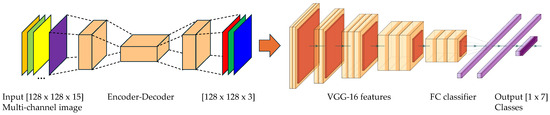
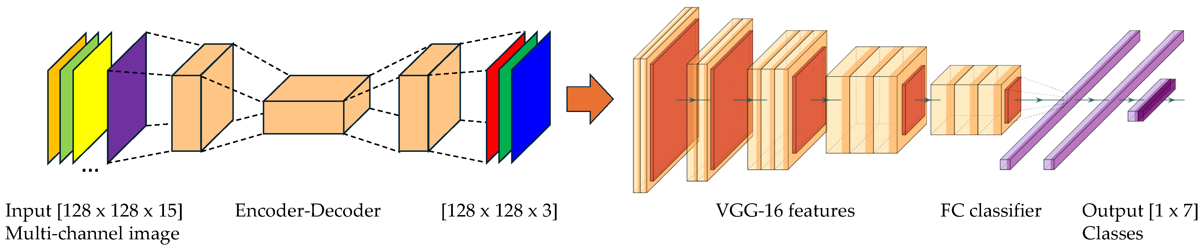
The proposed classification framework is implemented as a single end-to-end network composed of two main components (Figure 3): (i) a multispectral encoder–decoder module that maps the original multi-channel input into a three-channel representation, and (ii) a convolutional neural network pre-trained on RGB imagery, which serves as the classification backbone. The network operates on image tiles of size 128 × 128 pixels, with each pixel represented by a 15-dimensional feature vector comprising the 10 spectral bands and the 5 vegetation indices.
Figure 3.
Proposed classification network. The input is a multi-channel image composed of the spectral bands and vegetation indices. An encoder–decoder module first squeezes the input channels into a standard 3-channel representation, suitable for feeding into a pre-trained VGG-16 truncated at the feature extraction stage. The extracted features are then passed to a final fully connected classifier that assigns each tile to one of the 7 output classes.
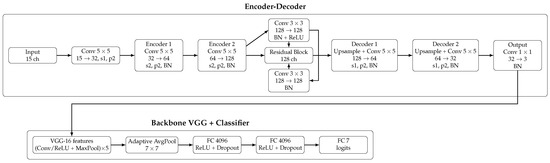
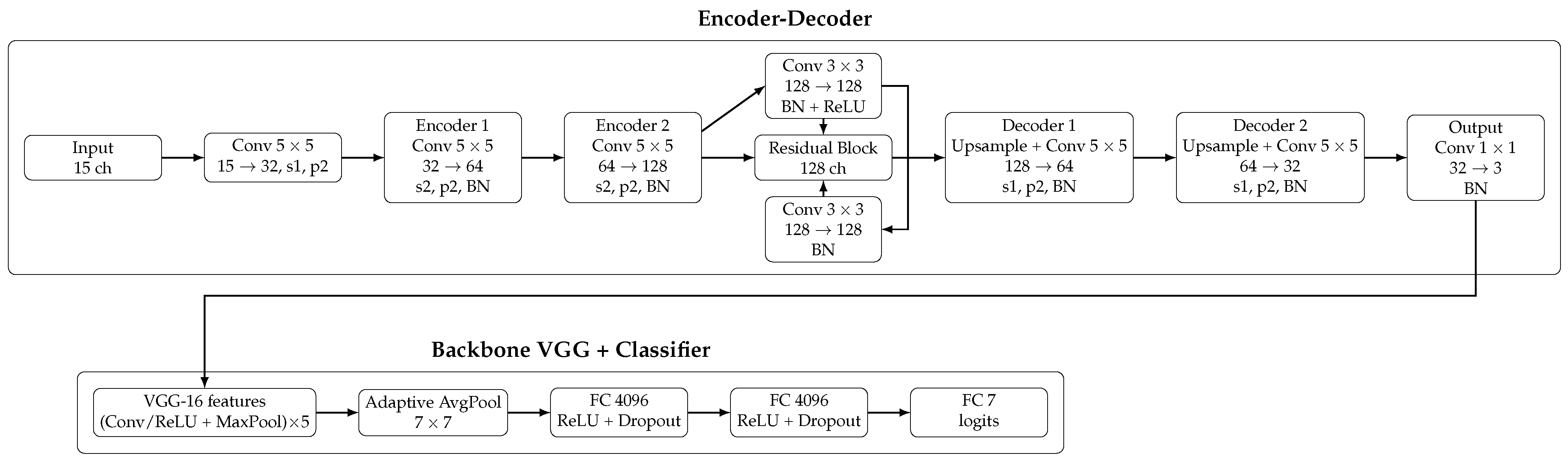
More in detail, the first component is a lightweight encoder–decoder network designed to reduce the channel dimensionality of the input while preserving its spatial structure. The module operates in a fully convolutional manner and processes entire image tiles simultaneously. As illustrated in Figure 4, the encoder consists of a sequence of convolutional layers with an increasing number of feature maps (32, 64, and 128 channels), combined with batch normalization. Spatial resolution is progressively reduced through strided convolutions, enabling the extraction of increasingly abstract spectral–spatial features. At the bottleneck, a residual block is introduced to facilitate gradient propagation and enhance training stability.
Figure 4.
Network architecture with detailed layer configuration. Conv: convolutional layer; BN: batch normalization; ReLU: rectified linear unit; MaxPool: max pooling; Adaptive AvgPool: adaptive average pooling; FC: fully connected layer; s: stride; p: padding; ch: number of feature channels.
The decoder mirrors the encoder structure and gradually restores the original spatial resolution through upsampling convolutional layers. Feature dimensionality is progressively reduced until a final convolutional layer produces a three-channel feature map with the same spatial dimensions as the input tile (128 × 128). This output can be interpreted as a learned pseudo-RGB representation, specifically optimized for the subsequent classification task. Batch normalization is applied throughout the encoder–decoder to improve convergence and robustness.
The second component of the architecture is based on the VGG-16 convolutional neural network [56], pre-trained on a large-scale RGB image dataset. The three-channel output produced by the multispectral encoding module is directly fed into the VGG-16 backbone, which preserves its original convolutional structure, consisting of five convolutional blocks with increasing feature depth, interleaved with rectified linear unit activations and max-pooling layers. Global feature aggregation is performed via adaptive average pooling, followed by two fully connected layers with dropout regularization to mitigate overfitting. The network is adapted to the salt marsh classification task by replacing the original output layer with a fully connected layer producing class scores for the seven target vegetation classes.
Training follows a transfer learning strategy in which the weights of the VGG-16 backbone are kept frozen, while the parameters of the multispectral encoder–decoder module and the final classification layers are optimized. This approach allows the model to exploit robust feature representations learned from large RGB datasets while limiting the number of trainable parameters and reducing the amount of annotated multispectral data required for effective learning. Importantly, the encoder–decoder module is not trained as a standalone autoencoder but is integrated directly into the classification network and optimized jointly with the classifier, ensuring that the learned three-channel representation is explicitly driven by the final classification objective.
The model was implemented using the PyTorch (version 2.5.0) framework [57]. The VGG-16 architecture and its ImageNet-1K pre-trained weights were obtained from the PyTorch Model Zoo. Network optimization was performed using the AdamW optimizer, with the cross-entropy loss function employed for multi-class classification. All experiments were conducted on a workstation equipped with an NVIDIA GeForce RTX 3070 GPU (NVIDIA Corporate, Santa Clara, CA, USA). This implementation and training setup follows widely adopted practices in deep learning studies, ensuring reproducibility and consistency with established methodologies.
2.5. Evaluation Protocol
To quantitatively assess the proposed deep learning framework, beyond qualitative visual inspection, the performance of the developed approach was evaluated through a comparative analysis against two widely used machine learning classifiers, namely Support Vector Machines and Random Forest, which were adopted as baseline methods. For the ML approaches, each image tile was represented by a feature vector obtained by averaging the values of the spectral bands and vegetation indices over all pixels within the tile.
To analyze the contribution of different spectral representations, an ablation study was also conducted. The DL model was evaluated under three alternative input configurations: (i) the complete input composed of 10 spectral bands and 5 vegetation indices (SB+VI), (ii) only the 10 spectral bands (SB), and (iii) only the 5 vegetation indices (VI). This analysis was designed to assess the relative impact of raw spectral information and derived vegetation indices on classification performance. For consistency, the same input configurations were also tested for the ML baseline methods (SVM and RF), and their results are reported for comparison.
Classification performance was quantified using standard multi-class evaluation metrics, including Overall Accuracy (OA), precision, recall, and F1-score. Overall Accuracy measures the proportion of correctly classified samples with respect to the total number of observations. Precision, recall, and F1-score were computed on a per-class basis and subsequently aggregated using both macro-averaging and weighted averaging. Macro-averaged metrics assign equal importance to all classes, whereas weighted averages account for class imbalance by weighting each class according to its relative frequency in the dataset. In addition, confusion matrices were analyzed to support the interpretation of class-specific errors and misclassification patterns.
For the quantitative comparison and ablation analysis, the ground-truth dataset was randomly split into a training set (90%) and a held-out test set (10%), while preserving the original class proportions. All performance metrics reported for these experiments were computed on the test set.
Finally, given the limited size of the dataset and its pronounced class imbalance (Table 1), a stratified 5-fold cross-validation strategy was adopted to more robustly assess the DL approach. The dataset was partitioned into five folds, each preserving the class distribution of the full dataset. At each iteration, four folds were used for training and the remaining fold for testing, and performance metrics were computed as the average across the five runs. This analysis was not extended to the ML baselines, as their performance was consistently and substantially lower in the comparative experiments, as reported in Section 3.2.
3. Results
3.1. Qualitative Classification Results
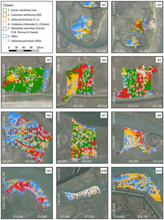
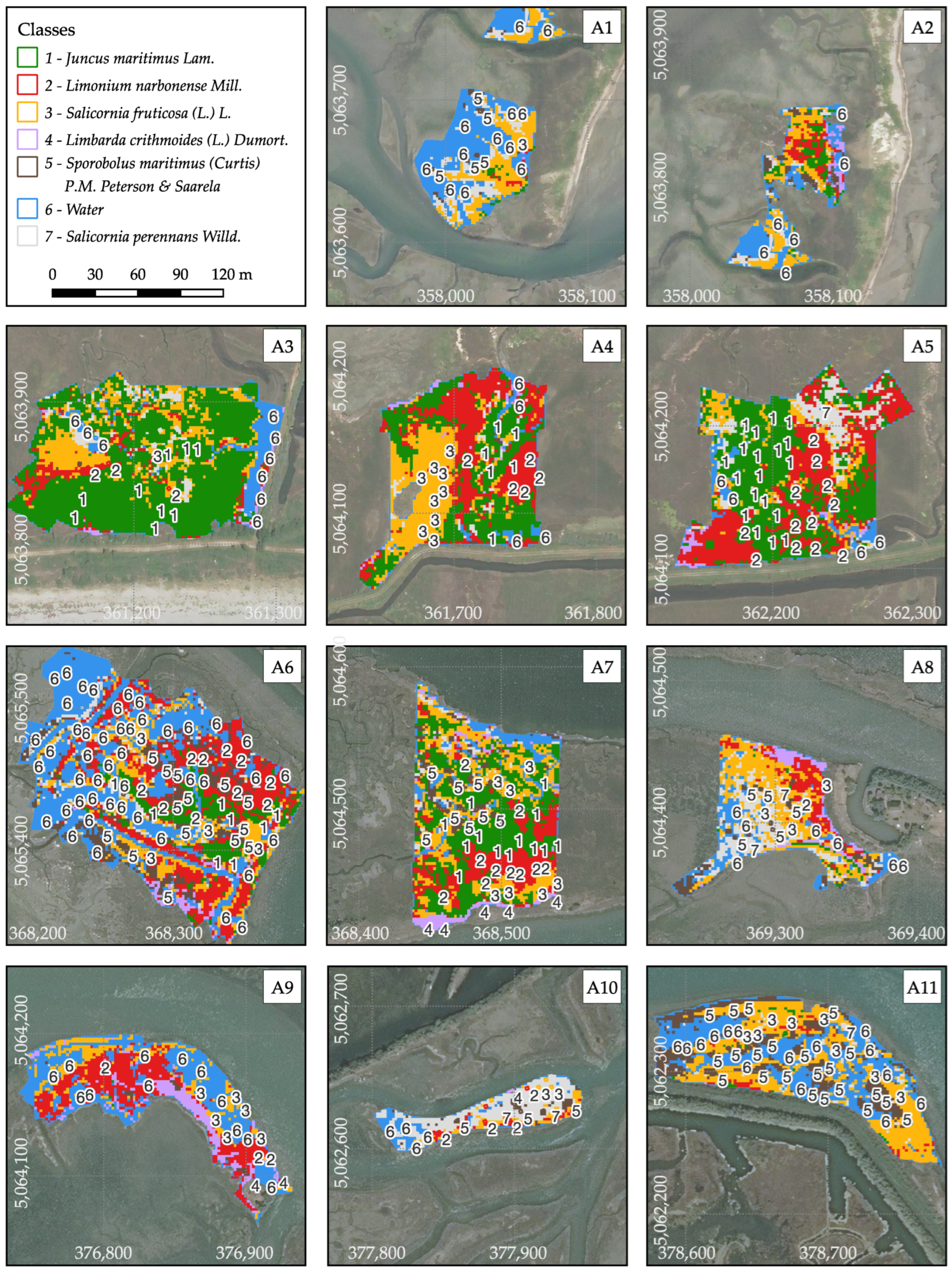
Figure 5 shows the classification results obtained with the proposed deep learning framework for all eleven study areas. The predicted maps exhibit a high degree of spatial coherence and reproduce the main spatial patterns typically observed in salt marsh environments. A qualitative assessment can be performed by visually comparing the classified maps with the ground-truth tiles superimposed in the figure. In most areas, the predicted classes are consistent with the reference samples, indicating a good agreement between the model output and the in situ observations used for training and testing. Dominant vegetation types and water bodies are generally well delineated, as illustrated, for example, in areas A1 and A9. In sites characterized by larger and more homogeneous patches, the classification appears particularly stable, whereas finer-scale spatial structures are preserved in areas exhibiting more fragmented vegetation mosaics (e.g., A6 and A7).
Figure 5.
Classification results obtained with the proposed deep learning framework for all study areas. Ground-truth field sampling plots (shown as small polygons) are overlaid on the classification maps. All areas are shown at the same scale, indicated in the upper-left box. The coordinates are expressed in meters in the RDN2008/UTM Zone 33N coordinate reference system (EPSG:6708). The satellite basemap is provided by Bing Maps.
These qualitative results provide an initial visual validation of the proposed method, which is further substantiated in the following sections through quantitative metrics and confusion matrix analysis.
3.2. Quantitative Comparison and Ablation Analysis
Table 3 reports the quantitative classification performance of the proposed deep learning framework and the machine learning baselines (SVM and RF) under the different input configurations.
Table 3.
Quantitative comparison of classification performance for the proposed DL model and the ML baselines (SVM and RF) under different input configurations. Overall Accuracy (OA) is reported together with Precision (Prec), Recall (Rec), and F1-score (F1); the latter metrics are provided using both macro-averaging and weighted-averaging to account for class imbalance. The bold values indicate the best performance for each metric.
Considering the DL approach, the highest performance is achieved when using the complete spectral configuration combining spectral bands and vegetation indices (SB+VI). In this setting, the model attains an Overall Accuracy of 0.984, with consistently high values across both macro-averaged and weighted-averaged metrics, all exceeding 0.98. When restricting the input to vegetation indices only (VI), the DL model still yields high classification accuracy (OA = 0.969), with a moderate reduction in macro-averaged precision and F1-score. Conversely, the configuration based solely on spectral bands (SB) results in a more pronounced decrease in performance, particularly in the macro-averaged metrics, indicating a less balanced classification across classes.
A clear performance gap is observed between the DL framework and the ML baselines across all input configurations. The SVM classifier achieves Overall Accuracy values ranging between 0.703 and 0.734, with relatively low macro-averaged F1-scores, reflecting difficulties in achieving balanced class-wise performance. The RF classifier consistently outperforms SVM, reaching an Overall Accuracy of 0.906 for both the SB+VI and SB configurations. Nevertheless, even in its best-performing setting, RF remains substantially below the performance achieved by the DL model using the full SB+VI input. Differences between macro-averaged and weighted-averaged metrics are more pronounced for the ML approaches, suggesting a stronger influence of class imbalance compared to the DL framework.
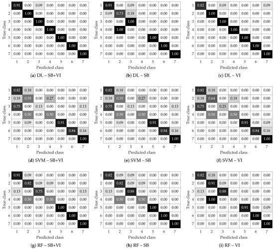
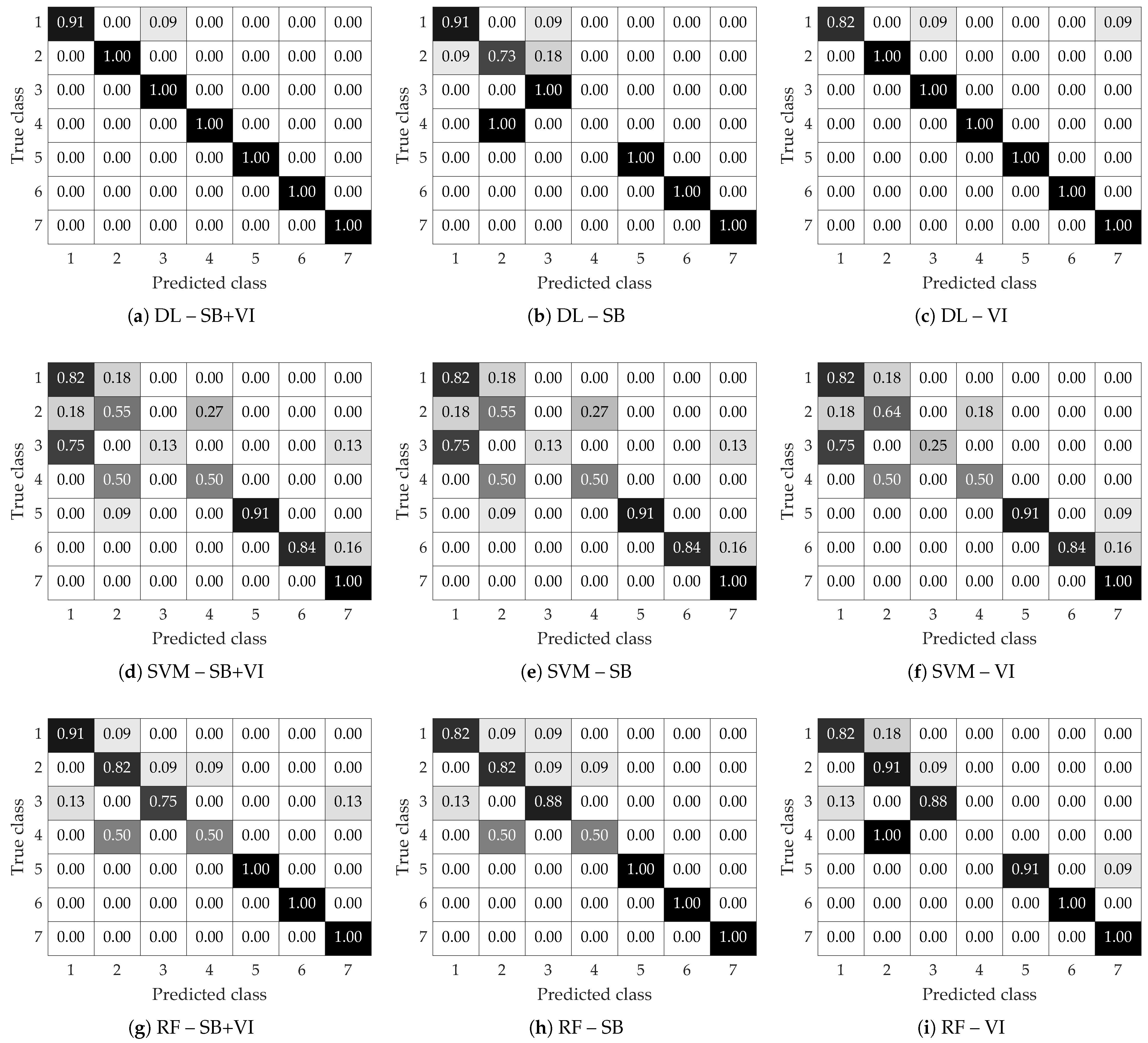
The normalized confusion matrices shown in Figure 6 provide a detailed, class-wise perspective on the classification behavior of the different methods and input configurations. For the proposed DL framework using the full SB+VI input (Figure 6a), the matrices exhibit a pronounced diagonal dominance across all classes, indicating a high proportion of correctly classified samples and a generally balanced performance. Misclassifications are limited and mainly involve minor confusions between spectrally similar vegetation classes.
Figure 6.
Normalized confusion matrices for the proposed DL model and the ML baselines (SVM and RF) under three input configurations: spectral bands and vegetation indices (SB+VI), spectral bands only (SB), and vegetation indices only (VI). Rows are ordered as DL, SVM, and RF, while columns are ordered as SB+VI, SB, and VI. All matrices are normalized by the number of samples per class. Values range from 0 to 1 and are reported within each cell; a common color scale is used across all images. The correspondence between class numbers and species is as follows: 1—Juncus maritimus Lam.; 2—Limonium narbonense Mill.; 3—Salicornia fruticosa (L.) L.; 4—Limbarda crithmoides (L.) Dumort.; 5—Sporobolus maritimus (Curtis) P.M. Peterson & Saarela; 6—Water; 7—Salicornia perennans Willd.
When the DL input is reduced to spectral bands only (Figure 6b) or vegetation indices only (Figure 6c), the overall diagonal structure is largely preserved, although an increase in off-diagonal elements becomes evident for specific classes. A closer examination reveals distinct misclassification patterns between the two reduced-input configurations. In the VI-only case, classification errors are primarily confined to class 1 (Juncus maritimus), while the remaining classes maintain a clear diagonal dominance. Conversely, the SB-only configuration shows a broader distribution of misclassifications affecting the first four classes, with class 4 (Limbarda crithmoides) being entirely misclassified and assigned to class 2 (Limonium narbonense).
By comparison, the confusion matrices obtained for the ML baseline methods (Figure 6d–i) display more pronounced off-diagonal patterns. The SVM classifier is characterized by frequent misclassifications across multiple vegetation classes, resulting in reduced class separability and lower class-wise recall, particularly for minority classes. Random Forest demonstrates improved diagonal dominance relative to SVM; however, noticeable confusions persist, especially among classes 1–4.
3.3. Cross-Validation Results
Table 4 summarizes the cross-validation results obtained using the three input settings. Overall, the DL model shows stable performance across folds for all configurations, with limited variability in terms of Overall Accuracy and macro-averaged metrics. The combined SB+VI input yields consistently high results, while the VI-only configuration achieves slightly higher mean values for OA, macro-precision, and macro-F1 score. Conversely, the SB-only configuration exhibits a modest reduction in performance, particularly in terms of recall and F1-score.
Table 4.
Stratified 5-fold cross-validation results for the proposed DL model using different input configurations. Values are reported as mean ± standard deviation of OA and macro-averaged precision, recall, and F1-score. The bold values indicate the best performance for each metric.
Despite these differences in average metrics, statistical analysis indicates that the performance variations between the SB+VI and VI-only configurations are not statistically significant. Both the Wilcoxon signed-rank test () and the paired t-test () fail to reject the null hypothesis, suggesting that the observed differences in performance between the two input configurations are within the variability captured by the cross-validation procedure.
4. Discussion
Overall, the results show that the proposed framework operates reliably across heterogeneous lagoon sectors with different spatial extents and degrees of class mixing. Predicted maps remain spatially coherent with the ground-truth tiles even in transitional zones, indicating stable performance under local spatial variability. Although the training dataset is relatively limited for deep learning, the confusion matrix and the quantitative results in Table 3 confirm the superior class-wise consistency of the proposed approach, especially with the SB+VI configuration. This highlights the difficulty of ML baselines in handling class imbalance and the spectral similarity typical of fine-grained salt marsh vegetation.
To mitigate biased estimates due to uneven class distribution, we evaluated the model using hold-out testing and a stratified 5-fold cross-validation scheme combined with a percentage-based train–test split at the tile level. Under the current data configuration (highly uneven spatial distribution and few plots for some classes), spatial hold-out strategies such as Leave-One-Area-Out can yield non-representative splits where some classes are poorly represented or absent, producing unstable or biased estimates. Stratified cross-validation instead ensures more balanced class representation and a more reliable assessment given the available ground truth.
The results support the main premise of this work: RGB-pretrained CNNs can be transferred to multispectral UAV data through an explicit spectral adaptation stage. The learnable encoder maps the 15-channel multispectral input into a three-channel representation compatible with an RGB-pretrained backbone (VGG-16) and is optimized end-to-end via the classification loss. While some raw spectral detail is necessarily compressed, the consistently high accuracy and strong macro-averaged metrics indicate that the learned representation preserves the information most relevant to discriminate the target classes. A key implication is data efficiency under constrained annotation. With 602 plots and imbalanced fine-grained classes, training a deep CNN from scratch would be unreliable; freezing the pretrained backbone and training only the encoder and classifier reduces the number of trainable parameters and helps mitigate overfitting while still adapting to the target spectral domain. This is particularly relevant for UAV-based ecological monitoring, where extensive in situ labeling is often impractical.
Salt marsh vegetation exhibits partially overlapping spectral responses, raising potential spectral confusion. In this framework, separability is not pursued through hand-crafted feature-space discrimination alone: the network learns a task-driven spectral–spatial transformation that enhances class separability in the learned representation, and separability is therefore assessed implicitly through performance metrics and confusion patterns rather than through standalone feature-level distances. In addition, performance gains over RF/SVM are attributable not only to spectral modeling but also to the ability of CNNs to exploit within-tile spatial context and texture, which are discarded by spatially averaged ML features.
The ablation analysis further supports the input design: combining spectral bands and vegetation indices yields the most robust and balanced performance, consistent with the complementary information carried by raw reflectance and index-based descriptors. While VI-only achieved competitive cross-validation results, SB+VI consistently performed best on held-out testing. Direct quantitative comparisons with prior studies remain difficult due to differences in class taxonomies, sensors, resolution, and evaluation protocols. Nevertheless, the achieved accuracy is within (and often above) the range commonly reported for multispectral UAV salt marsh classification, suggesting that the proposed strategy is competitive under current practice.
Despite the strong performance achieved, some limitations should be acknowledged. First, the framework was tested on a single lagoon system and one sensor; transferability to other sites, sensors, and acquisition conditions was not explicitly evaluated. Future work will extend experiments to multiple salt marsh systems and more diverse datasets: with more spatially balanced sampling, spatial generalization tests (including Leave-One-Area-Out) will become feasible and more informative.
Second, classification is performed at the tile level (dominant-class labeling). This increases robustness to pixel-level noise but can smooth fine boundaries and introduce mixed-class effects in highly heterogeneous tiles. Future work will investigate semantic segmentation to enable pixel-level mapping and to address pixel mixing more explicitly.
Third, the 15-to-3 channel compression enables reuse of RGB backbones but constrains how spectral information is represented. Future analyses will focus on interpretability (e.g., visualization/sensitivity of pseudo-RGB channels) and on alternative adaptation strategies that preserve additional spectral degrees of freedom while retaining the benefits of RGB pretraining.
Finally, the modular encoder design supports extensions such as alternative band configurations, inclusion of additional vegetation indices, and multi-source data fusion, which may further improve scalability for long-term coastal wetland monitoring.
5. Conclusions
This study proposed a deep learning framework for the classification of salt marsh vegetation from UAV-based multispectral imagery, leveraging transfer learning from convolutional neural networks pre-trained on large RGB image datasets. The core contribution lies in the introduction of a learnable spectral encoding module that maps multispectral inputs, including vegetation indices, into a three-channel representation compatible with an RGB-trained backbone. This strategy enables the effective reuse of established CNN architectures, such as VGG-16, while mitigating the need for large annotated multispectral training datasets.
The experimental results demonstrate that the proposed approach consistently outperforms traditional machine learning classifiers, including Support Vector Machines and Random Forest, across all evaluated input configurations. In particular, the joint use of spectral bands and vegetation indices leads to the highest classification performance, achieving an Overall Accuracy of 98.4% and improved class-wise consistency despite pronounced class imbalance. The robustness of the framework is further supported by stratified cross-validation, showing stable performance across different data partitions. The ablation analysis highlights that vegetation indices provide complementary information that enhances class separability beyond what can be achieved using spectral bands alone.
These findings confirm that RGB-pretrained convolutional neural networks can be successfully adapted to multispectral UAV data through an appropriate spectral transformation, even under constrained training conditions. By limiting the number of trainable parameters and exploiting both spectral and spatial information at the tile level, the proposed framework offers a data-efficient and reliable solution for high-resolution vegetation mapping in heterogeneous salt marsh environments.
Overall, the proposed approach represents a competitive and transferable methodology for multispectral vegetation classification, with direct relevance for ecological monitoring and coastal management applications. The modular design of the spectral encoding component facilitates adaptation to different multispectral sensors and acquisition settings, providing a solid foundation for future extensions aimed at improving generalization across sites, sensors, and environmental conditions.
Author Contributions
Conceptualization, S.O.M., E.M. and A.F.; methodology, S.O.M., E.M. and A.F.; software, S.O.M.; validation, E.M. and A.F.; formal analysis, E.M. and A.F.; investigation, E.M., P.C., G.T., M.V. and A.F.; data curation, P.C., G.T. and M.V.; writing—original draft preparation, E.M. and A.F.; writing—review and editing, S.O.M., E.M., F.B., P.C., F.T., M.V. and A.F.; visualization, E.M. and A.F.; supervision, F.B., F.T. and A.F.; project administration, F.B. and F.T.; funding acquisition, F.B. and F.T. All authors have read and agreed to the published version of the manuscript.
Funding
This research was carried out within the framework of the INTERREG VIA IT-HR BRIGANTINE project (ID ITHR0200237) and was supported by the strategic plan of the University of Udine (DPIA) under the AMARE project. This activity was also part of the National Biodiversity Future Center (NBFC), project funded by the European Union—NextGenerationEU under the National Recovery and Resilience Plan (NRRP), Mission 4, Component 2, Investment 1.4—Call for tender No. 3138 of 16 December 2021, rectified by Decree n.3175 of 18 December 2021 of Italian Ministry of University and Research (project code CN_00000033).
Institutional Review Board Statement
Not applicable.
Informed Consent Statement
Not applicable.
Data Availability Statement
The datasets produced in this study are available from the authors upon request.
Conflicts of Interest
The authors declare no conflicts of interest.
Abbreviations
The following abbreviations are used in this manuscript:
| Blue | |
| Convolutional Neural Network | CNN |
| Deep Learning | DL |
| Downwelling Light Sensor | DLS |
| Enhanced Vegetation Index | EVI |
| F1-score | F1 |
| Full Width at Half Maximum | FWHM |
| Global Navigation Satellite System | GNSS |
| Green | |
| Green Normalized Difference Vegetation Index | GNDVI |
| Ground Sampling Distance | GSD |
| Machine Learning | ML |
| Modified Soil Adjusted Vegetation Index | MSAVI |
| Near-infrared | |
| Normalized Difference Red Edge Index | NDRE |
| Normalized Difference Vegetation Index | NDVI |
| Normalized Difference Water Index | NDWI |
| Overall Accuracy | OA |
| Precision | Prec |
| Random Forest | RF |
| Recall | Rec |
| Red | |
| Red-edge | |
| Spectral Angle Mapper | SAM |
| Spectral Band | SB |
| Support Vector Machine | SVM |
| Uncrewed Aerial Vehicle | UAV |
| Vegetation Index | VI |
References
- Barnes, R.S.K. The coastal lagoons of Britain: An overview and conservation appraisal. Biol. Conserv. 1989, 49, 295–313. [Google Scholar] [CrossRef] [Scilit]
- Kjerfve, B. Coastal Lagoons; Elsevier oceanography series; Elsevier: Amsterdam, The Netherlands, 1994; Volume 60, pp. 1–8. [Google Scholar]
- Orchard, S.; Hughey, K.F.D.; Schiel, D.R. Risk factors for the conservation of saltmarsh vegetation and blue carbon revealed by earthquake-induced sea-level rise. Sci. Total Environ. 2020, 746, 141241. [Google Scholar] [CrossRef] [Scilit]
- Barnes, R.S.K. Coastal Lagoons; Cambridge University Press: Cambridge, UK, 1980; Volume 1. [Google Scholar]
- Pérez-Ruzafa, A.; Marcos, C.; Pérez-Ruzafa, I.M. Mediterranean coastal lagoons in an ecosystem and aquatic resources management context. Phys. Chem. Earth Parts a/b/c 2011, 36, 160–166. [Google Scholar] [CrossRef] [Scilit]
- Bas-Silvestre, M.; Quintana, X.D.; Compte, J.; Gascon, S.; Boix, D.; Anton-Pardo, M.; Obrador, B. Ecosystem metabolism dynamics and environmental drivers in Mediterranean confined coastal lagoons. Estuar. Coast. Shelf Sci. 2020, 245, 106989. [Google Scholar] [CrossRef] [Scilit]
- Cingano, P.; Vuerich, M.; Petruzzellis, F.; Orzan, L.; Trotta, G.; Casolo, V.; Asquini, E.; Bacaro, G.; Boscutti, F. Seagrasses on the move: Tracing the multi-decadal species distribution trends in lagoon meadows using Landsat imagery. Ecol. Inform. 2024, 82, 102685. [Google Scholar] [CrossRef] [Scilit]
- Franco, A.; Franzoi, P.; Malavasi, S.; Riccato, F.; Torricelli, P.; Mainardi, D. Use of shallow water habitats by fish assemblages in a Mediterranean coastal lagoon. Estuar. Coast. Shelf Sci. 2006, 66, 67–83. [Google Scholar] [CrossRef] [Scilit]
- Giordano, J.C.P.; Brush, M.J.; Anderson, I.C. Ecosystem metabolism in shallow coastal lagoons: Patterns and partitioning of planktonic, benthic, and integrated community rates. Mar. Ecol. Prog. Ser. 2012, 458, 21–38. [Google Scholar] [CrossRef] [Scilit]
- Newton, A.; Brito, A.C.; Icely, J.D.; Derolez, V.; Clara, I.; Angus, S.; Schernewski, G.; Inácio, M.; Lillebø, A.I.; Sousa, A.I.; et al. Assessing, quantifying and valuing the ecosystem services of coastal lagoons. J. Nat. Conserv. 2018, 44, 50–65. [Google Scholar] [CrossRef] [Scilit]
- Albert, S.; Saunders, M.I.; Roelfsema, C.M.; Leon, J.X.; Johnstone, E.; Mackenzie, J.R.; Hoegh-Guldberg, O.; Grinham, A.R.; Phinn, S.R.; Duke, N.C.; et al. Winners and losers as mangrove, coral and seagrass ecosystems respond to sea-level rise in Solomon Islands. Environ. Res. Lett. 2017, 12, 094009. [Google Scholar] [CrossRef] [Scilit]
- Morris, J.T.; Sundareshwar, P.V.; Nietch, C.T.; Kjerfve, B.; Cahoon, D.R. Responses of coastal wetlands to rising sea level. Ecology 2002, 83, 2869–2877. [Google Scholar] [CrossRef]
- Newton, A.; Icely, J.; Cristina, S.; Brito, A.C.; Cardoso, A.C.; Colijn, F.; Dalla Riva, S.; Gertz, F.; Hansen, J.W.; Holmer, M.; et al. An overview of ecological status, vulnerability and future perspectives of European large shallow, semi-enclosed coastal systems, lagoons and transitional waters. Estuar. Coast. Shelf Sci. 2014, 140, 95–122. [Google Scholar] [CrossRef] [Scilit]
- Sarretta, A.; Pillon, S.; Molinaroli, E.; Guerzoni, S.; Fontolan, G. Sediment budget in the Lagoon of Venice, Italy. Cont. Shelf Res. 2010, 30, 934–949. [Google Scholar] [CrossRef] [Scilit]
- Waycott, M.; Duarte, C.M.; Carruthers, T.J.; Orth, R.J.; Dennison, W.C.; Olyarnik, S.; Calladine, A.; Fourqurean, J.W.; Heck, K.L., Jr.; Hughes, A.R.; et al. Accelerating loss of seagrasses across the globe threatens coastal ecosystems. Proc. Natl. Acad. Sci. USA 2009, 106, 12377–12381. [Google Scholar] [CrossRef] [Scilit]
- Suresh, K.; Khanal, U.; Wilson, C. Stakeholders’ use and preservation valuation of lagoon ecosystems. Econ. Anal. Policy 2021, 71, 123–137. [Google Scholar] [CrossRef] [Scilit]
- Boorman, L.A. Saltmarsh Review: An Overview of Coastal Saltmarshes, Their Dynamic and Sensitivity Characteristics for Conservation and Management; Technical Report 334; JNCC: Peterborough, UK, 2003. [Google Scholar]
- Bockelmann, A.C.; Bakker, J.P.; Neuhaus, R.; Lage, J. The relation between vegetation zonation, elevation and inundation frequency in a Wadden Sea salt marsh. Aquat. Bot. 2002, 73, 211–221. [Google Scholar] [CrossRef] [Scilit]
- Pellegrini, E.; Boscutti, F.; De Nobili, M.; Casolo, V. Plant traits shape the effects of tidal flooding on soil and plant communities in saltmarshes. Plant Ecol. 2018, 219, 823–835. [Google Scholar] [CrossRef] [Scilit]
- Barbier, E.B.; Hacker, S.D.; Kennedy, C.; Koch, E.W.; Stier, A.C.; Silliman, B.R. The value of estuarine and coastal ecosystem services. Ecol. Monogr. 2011, 81, 169–193. [Google Scholar] [CrossRef] [Scilit]
- Vuerich, M.; Cingano, P.; Trotta, G.; Petrussa, E.; Braidot, E.; Scarpin, D.; Bezzi, A.; Mestroni, M.; Pellegrini, E.; Boscutti, F. New perspective for the upscaling of plant functional response to flooding stress in salt marshes using remote sensing. Sci. Rep. 2024, 14, 5472. [Google Scholar] [CrossRef] [Scilit] [PubMed]
- Klemas, V. Remote sensing of emergent and submerged wetlands: An overview. Int. J. Remote Sens. 2013, 34, 6286–6320. [Google Scholar] [CrossRef] [Scilit]
- Turner, I.L.; Harley, M.D.; Drummond, C.D. UAVs for coastal surveying. Coast. Eng. 2016, 114, 19–24. [Google Scholar] [CrossRef] [Scilit]
- Belluco, E.; Camuffo, M.; Ferrari, S.; Modenese, L.; Silvestri, S.; Marani, A.; Marani, M. Mapping salt-marsh vegetation by multispectral and hyperspectral remote sensing. Remote Sens. Environ. 2006, 105, 54–67. [Google Scholar] [CrossRef] [Scilit]
- Yeo, S.; Lafon, V.; Alard, D.; Curti, C.; Dehouck, A.; Benot, M.L. Classification and mapping of saltmarsh vegetation combining multispectral images with field data. Estuar. Coast. Shelf Sci. 2020, 236, 106643. [Google Scholar] [CrossRef] [Scilit]
- Sun, C.; Fagherazzi, S.; Liu, Y. Classification mapping of salt marsh vegetation by flexible monthly NDVI time-series using Landsat imagery. Estuar. Coast. Shelf Sci. 2018, 213, 61–80. [Google Scholar] [CrossRef] [Scilit]
- Zhang, C.; Gong, Z.; Qiu, H.; Zhang, Y.; Zhou, D. Mapping typical salt-marsh species in the Yellow River Delta wetland supported by temporal-spatial-spectral multidimensional features. Sci. Total Environ. 2021, 783, 147061. [Google Scholar] [CrossRef] [Scilit] [PubMed]
- Norris, G.S.; LaRocque, A.; Leblon, B.; Barbeau, M.A.; Hanson, A.R. Comparing pixel-and object-based approaches for classifying multispectral drone imagery of a salt marsh restoration and reference site. Remote Sens. 2024, 16, 1049. [Google Scholar] [CrossRef] [Scilit]
- Rouse, J.W., Jr.; Haas, R.H.; Deering, D.W.; Schell, J.A.; Harlan, J.C. Monitoring the Vernal Advancement and Retrogradation (Green Wave Effect) of Natural Vegetation; Technical Report No. E75-10354; Remote Sensing Center, Texas A&M University: College Station, TX, USA, 1973. [Google Scholar]
- Gitelson, A.A.; Kaufman, Y.J.; Merzlyak, M.N. Use of a green channel in remote sensing of global vegetation from EOS-MODIS. Remote Sens. Environ. 1996, 58, 289–298. [Google Scholar] [CrossRef] [Scilit]
- Qi, J.; Chehbouni, A.; Huete, A.R.; Kerr, Y.H.; Sorooshian, S. A modified soil adjusted vegetation index. Remote Sens. Environ. 1994, 48, 119–126. [Google Scholar] [CrossRef] [Scilit]
- Xue, J.; Su, B. Significant remote sensing vegetation indices: A review of developments and applications. J. Sens. 2017, 2017, 1353691. [Google Scholar] [CrossRef] [Scilit]
- Myers, D.; Schweik, C.; Wicks, R.; Bowlick, F.; Carullo, M. Developing a land cover classification of salt marshes using UAS time-series imagery and an open source workflow. Int. Arch. Photogramm. Remote Sens. Spat. Inf. Sci. 2018, 42, 155–162. [Google Scholar] [CrossRef] [Scilit]
- Routhier, M.; Moore, G.; Rock, B. Assessing spectral band, elevation, and collection date combinations for classifying salt marsh vegetation with unoccupied aerial vehicle (UAV)-acquired imagery. Remote Sens. 2023, 15, 5076. [Google Scholar] [CrossRef] [Scilit]
- Belcore, E.; Latella, M.; Piras, M.; Camporeale, C. Enhancing precision in coastal dunes vegetation mapping: Ultra-high resolution hierarchical classification at the individual plant level. Int. J. Remote Sens. 2024, 45, 4527–4552. [Google Scholar] [CrossRef] [Scilit]
- Xu, R.; Fan, Y.; Fan, B.; Feng, G.; Li, R. Classification and monitoring of salt marsh vegetation in the Yellow River Delta based on multi-source remote sensing data fusion. Sensors 2025, 25, 529. [Google Scholar] [CrossRef] [Scilit] [PubMed]
- Norris, G.; Leblon, B.; LaRocque, A.; Barbeau, M.; Hanson, A. Effect of textural features for landcover classification of UAV multispectral imagery of a salt marsh restoration site. Int. Arch. Photogramm. Remote Sens. Spat. Inf. Sci. 2022, 43, 951–958. [Google Scholar] [CrossRef] [Scilit]
- Curcio, A.C.; Barbero, L.; Peralta, G. UAV-hyperspectral imaging to estimate species distribution in salt marshes: A case study in the Cadiz Bay (SW Spain). Remote Sens. 2023, 15, 1419. [Google Scholar] [CrossRef] [Scilit]
- Zheng, J.; Sun, C.; Zhao, S.; Hu, M.; Zhang, S.; Li, J. Classification of salt marsh vegetation in the Yangtze River Delta of China using the pixel-level time-series and XGBoost algorithm. J. Remote Sens. 2023, 3, 0036. [Google Scholar] [CrossRef] [Scilit]
- Li, H.; Wang, C.; Cui, Y.; Hodgson, M. Mapping salt marsh along coastal South Carolina using U-Net. ISPRS J. Photogramm. Remote Sens. 2021, 179, 121–132. [Google Scholar] [CrossRef] [Scilit]
- Zheng, J.Y.; Hao, Y.Y.; Wang, Y.C.; Zhou, S.Q.; Wu, W.B.; Yuan, Q.; Gao, Y.; Guo, H.Q.; Cai, X.X.; Zhao, B. Coastal wetland vegetation classification using pixel-based, object-based and deep learning methods based on RGB-UAV. Land 2022, 11, 2039. [Google Scholar] [CrossRef] [Scilit]
- Bai, X.; Yang, C.; Fang, L.; Chen, J.; Wang, X.; Gao, N.; Zheng, P.; Wang, G.; Wang, Q.; Ren, S. Identification of salt marsh vegetation in the Yellow River Delta using UAV multispectral imagery and Deep Learning. Drones 2025, 9, 235. [Google Scholar] [CrossRef] [Scilit]
- Ma, Y.; Chen, S.; Ermon, S.; Lobell, D.B. Transfer learning in environmental remote sensing. Remote Sens. Environ. 2024, 301, 113924. [Google Scholar] [CrossRef] [Scilit]
- He, X.; Chen, Y.; Ghamisi, P. Heterogeneous transfer learning for hyperspectral image classification based on convolutional neural network. IEEE Trans. Geosci. Remote Sens. 2019, 58, 3246–3263. [Google Scholar] [CrossRef] [Scilit]
- Li, Y.; Fu, B.; Sun, X.; Fan, D.; Wang, Y.; He, H.; Gao, E.; He, W.; Yao, Y. Comparison of different transfer learning methods for classification of mangrove communities using MCCUNet and UAV multispectral images. Remote Sens. 2022, 14, 5533. [Google Scholar] [CrossRef] [Scilit]
- Rise, B.; Uney, M.; Huang, X. Two-stage transfer learning for airborne multi-spectral image classifiers. Signal Process. 2025, 240, 110358. [Google Scholar] [CrossRef] [Scilit]
- Patel, U.; Pathan, M.; Kathiria, P.; Patel, V. Crop type classification with hyperspectral images using deep learning: A transfer learning approach. Model. Earth Syst. Environ. 2023, 9, 1977–1987. [Google Scholar] [CrossRef] [Scilit]
- Fontolan, G.; Pillon, S.; Bezzi, A.; Villalta, R.; Lipizer, M.; Triches, A.; D’Aietti, A. Human impact and the historical transformation of saltmarshes in the Marano and Grado Lagoon, northern Adriatic Sea. Estuar. Coast. Shelf Sci. 2012, 113, 41–56. [Google Scholar] [CrossRef] [Scilit]
- Bartolucci, F.; Peruzzi, L.; Galasso, G.; Albano, A.; Alessandrini, A.; Ardenghi, N.M.G.; Astuti, G.; Bacchetta, G.; Ballelli, S.; Banfi, E.; et al. An updated checklist of the vascular flora native to Italy. Plant Biosyst.- Int. J. Deal. All Asp. Plant Biol. 2018, 152, 179–303. [Google Scholar] [CrossRef] [Scilit]
- Rajakumari, S.; Mahesh, R.; Sarunjith, K.J.; Ramesh, R. Building spectral catalogue for salt marsh vegetation, hyperspectral and multispectral remote sensing. Reg. Stud. Mar. Sci. 2022, 53, 102435. [Google Scholar] [CrossRef] [Scilit]
- Pennings, S.C.; Callaway, R.M. Salt marsh plant zonation: The relative importance of competition and physical factors. Ecology 1992, 73, 681–690. [Google Scholar] [CrossRef] [Scilit]
- Barnes, E.M.; Clarke, T.R.; Richards, S.E.; Colaizzi, P.D.; Haberland, J.; Kostrzewski, M.; Waller, P.; Choi, C.; Riley, E.; Thompson, T. Coincident detection of crop water stress, nitrogen status and canopy density using ground based multispectral data. In Proceedings of the Fifth International Conference on Precision Agriculture, Bloomington, MN, USA, 16–19 July 2000; Volume 1619. [Google Scholar]
- McFeeters, S.K. The use of the Normalized Difference Water Index (NDWI) in the delineation of open water features. Int. J. Remote Sens. 1996, 17, 1425–1432. [Google Scholar] [CrossRef] [Scilit]
- Huete, A.; Didan, K.; Miura, T.; Rodriguez, E.P.; Gao, X.; Ferreira, L.G. Overview of the radiometric and biophysical performance of the MODIS vegetation indices. Remote Sens. Environ. 2002, 83, 195–213. [Google Scholar] [CrossRef] [Scilit]
- Wang, L.; Wang, J.; Liu, Z.; Zhu, J.; Qin, F. Evaluation of a deep-learning model for multispectral remote sensing of land use and crop classification. Crop J. 2022, 10, 1435–1451. [Google Scholar] [CrossRef] [Scilit]
- Simonyan, K.; Zisserman, A. Very deep convolutional networks for large-scale image recognition. arXiv 2014, arXiv:1409.1556. [Google Scholar]
- Ansel, J.; Yang, E.; He, H.; Gimelshein, N.; Jain, A.; Voznesensky, M.; Bao, B.; Bell, P.; Berard, D.; Burovski, E.; et al. Pytorch 2: Faster machine learning through dynamic python bytecode transformation and graph compilation. In Proceedings of the 29th ACM International Conference on Architectural Support for Programming Languages and Operating Systems, La Jolla, CA, USA, 27 April–1 May 2024; Volume 2, pp. 929–947. [Google Scholar]

Disclaimer/Publisher’s Note: The statements, opinions and data contained in all publications are solely those of the individual author(s) and contributor(s) and not of MDPI and/or the editor(s). MDPI and/or the editor(s) disclaim responsibility for any injury to people or property resulting from any ideas, methods, instructions or products referred to in the content. |
© 2026 by the authors. Licensee MDPI, Basel, Switzerland. This article is an open access article distributed under the terms and conditions of the Creative Commons Attribution (CC BY) license.