A Configuration Optimization Method Based on Decoupled Recursive Strategy for Distributed UAV SAR 3D Imaging System

Highlights

What are the main findings?

• A configuration optimization model is established for distributed UAV SAR 3D imaging, jointly optimizing sensing performance and UAV compactness under practical constraints.
• A decoupled recursive strategy is proposed, decomposing the 3D problem into a continuous subproblem and a recursive procedure, thereby enhancing solution capability and efficiency.

What are the implications of the main findings?

• We improve the 3D reconstruction capability of distributed UAV SAR systems under complex practical constraints.
• We reduce the meta-heuristic optimization dimensionality from 3D to 1D, accelerating processing speed while avoiding challenges from the highly fragmented feasible region to ensure robust global performance.

Abstract

Compared with conventional synthetic aperture radar (SAR) three-dimensional (3D) imaging systems, distributed unmanned aerial vehicle (UAV) SAR systems offer enhanced flexibility and single-pass capability, enabling rapid 3D imaging. Their performance, however, critically depends on the spatial arrangement of UAVs. Improper configurations result in grating lobes and increase the sidelobe level, thereby degrading elevation reconstruction. Additionally, the coordinated operation of distributed UAVs imposes spatial constraints such as safety separation. To address these challenges, this paper formulates the configuration design as a multi-constraint, multi-objective optimization problem that simultaneously considers both imaging performance and operational feasibility. Based on compressive sensing (CS) theory, the influence of configuration on sparse imaging is analyzed, and practical constraints are integrated, including 3D span limits, safety separation, and mainlobe avoidance. A joint optimization model is established to minimize the cumulative coherence of the sensing matrix while maximizing system spatial compactness. To efficiently solve this high-dimensional problem, a decoupled recursive strategy is proposed. In the first stage, a hybrid algorithm combining particle swarm optimization (PSO) and covariance matrix adaptation evolution strategy (CMA-ES) performs global optimization in the baseline domain. In the second stage, a compact configuration is constructed within the feasible region via analytical spatial recursion. Experimental results demonstrate that the proposed approach effectively reduces sensing matrix coherence and improves 3D reconstruction quality.

1. Introduction

Due to the projection imaging principle of conventional two-dimensional (2D) synthetic aperture radar (SAR), geometric distortion of elevated targets is inherent. This effect is particularly pronounced when imaging complex urban scenes with buildings, where severe layover and shadowing degrade image interpretability [1]. To address this issue, Tomographic SAR (TomoSAR) forms an aperture in the elevation direction and enables three-dimensional (3D) imaging, thereby reconstructing the volumetric scattering structure of the target. As a result, TomoSAR has become an important research direction with broad applications in areas such as urban remote sensing [2,3] and forest surveying [4,5,6].

Conventional TomoSAR 3D imaging systems mainly fall into two modes: multi-pass SAR and array SAR. Multi-pass SAR relies on repeated flights [7,8,9], while array SAR systems utilize multiple array elements for echo reception [10,11,12], to synthesize an aperture in the elevation direction, and obtain elevation resolution. A distributed UAV 3D imaging system provides a new approach for rapid acquisition of 3D scattering information, due to flexible configuration and the ability to collect data within a single flight [13]. With features such as low deployment cost [14] and rapid imaging [15], it has been recognized as one of the promising directions for future 3D SAR systems [16].

In recent years, the performance of TomoSAR 3D imaging has been significantly enhanced through advanced signal reconstruction and post-processing techniques. For example, recent studies have introduced non-convex matrix completion to improve super-resolution capabilities [17], implemented new target detection architectures to handle model mismatch at large incidence angles [18], and developed weighted PGA methods for precise phase calibration [19]. While these signal-level advancements push the boundaries of image quality, the fundamental reconstruction performance remains intrinsically limited by the properties of the sensing matrix, which is dictated by the physical system configuration. Therefore, developing a robust configuration optimization strategy is vital for distributed UAV SAR systems.

Limited by factors such as cost and control accuracy, elevation sampling points in distributed UAV TomoSAR are often sparse. Therefore, compressive sensing (CS), as the underlying theory for sparse signal recovery, is used to process 3D signals [20]. The reconstruction performance of CS algorithms is closely related to the properties of the sensing matrix. Specifically, a necessary and sufficient condition for accurate reconstruction of the original signal is that the sensing matrix satisfies the restricted isometry property (RIP) [21,22]. In practice, because the RIP of the sensing matrix is difficult to verify, correlation is commonly used to evaluate the performance of the sensing matrix [23,24]. According to the principle of SAR 3D sparse imaging, the baseline distribution directly affects the sensing matrix. For a distributed UAV SAR 3D imaging system, baselines are obtained by mapping from the 3D configuration. An improper configuration degrades the sensing matrix, leading to a higher error rate in 3D reconstruction [13,25]. Therefore, configuration optimization is critical to ensure the 3D imaging performance of a distributed UAV SAR 3D imaging system.

In performance modeling and baseline optimization design for TomoSAR, some studies proceed by building on observation geometry [26] and parameter estimation bounds [20,27] in order to quantitatively characterize the relationship between baseline configuration and 3D imaging performance. Furthermore, other studies adopt criteria including sensing matrix coherence [28], elevation point spread function sidelobe metrics [29], and equivalent elevation resolution [30] to design and optimize baseline distributions.

In configuration optimization for distributed 3D SAR, existing research primarily focuses on spaceborne formations. Based on criteria such as tomographic sampling conditions, ambiguity free height, Cramer–Rao Lower Bound (CRLB), and engineering safety constraints, these studies jointly design elevation sampling and data acquisition, developing methods for orbit and formation geometry design [13,27,29,31]. For distributed UAV configuration optimization, Ref. [13] directly links 3D imaging quality to geometric arrangement and optimizes the equivalent baseline distribution to improve sparse 3D reconstruction performance. Ref. [32] considers inter platform safety separation while satisfying imaging conditions and proposes a UAV SAR distribution scheme that can be implemented in a single flight. Nevertheless, for performance optimization of distributed SAR 3D imaging systems under multiple constraints, systematic configuration designs remain limited.

In practical deployments, cooperative flight of multiple UAVs is subject to various constraints, including safety separation and spatial limits imposed by mission requirements. As a result, configuration optimization becomes a complex problem with multiple variables and multiple constraints coupled in 3D space. In this setting, the feasible region becomes discrete and has a fragmented nature due to constraints such as safety separation and mainlobe avoidance, meaning that conventional metaheuristic search methods often suffer from reduced search efficiency and a tendency to converge to local optima.

This paper studies the configuration design of distributed UAV SAR for 3D imaging within a volumetric observation space (Oxyz). First, the impact of configuration on 3D sparse imaging is analyzed through the properties of the sensing matrix. Key practical constraints of 3D spatial span, safety separation, and antenna mainlobe avoidance are then incorporated into a multi-objective optimization model that jointly improves sensing matrix performance and system compactness. To solve this high-dimensional problem efficiently and avoid local optima in fragmented feasible regions, a decoupled recursive strategy is proposed. It decomposes the 3D optimization into two stages: (1) one-dimensional (1D) baseline optimization using a hybrid PSO-CMA-ES algorithm, and (2) configuration--space mapping via analytical recursion from a fixed anchor point. A quadtree-based backtracking mechanism is also introduced to prevent deadlock during recursion. Together, this approach enables efficient configuration optimization under engineering constraints, thereby supporting accurate 3D inversion in complex scenes.

The remainder of this paper is organized as follows. In Section 2, the influence of configuration on imaging performance is analyzed. In Section 3, the configuration optimization problem for distributed UAV SAR under multiple constraints is formulated. In Section 4, the proposed optimization strategy and the complete procedure are presented. In Section 5, simulation results are provided. The effectiveness of the proposed method is validated in Section 6. In Section 7, the conclusions of the paper are presented.

2. The 3D SAR Imaging Configuration Model

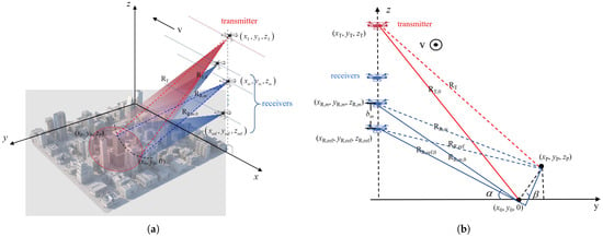
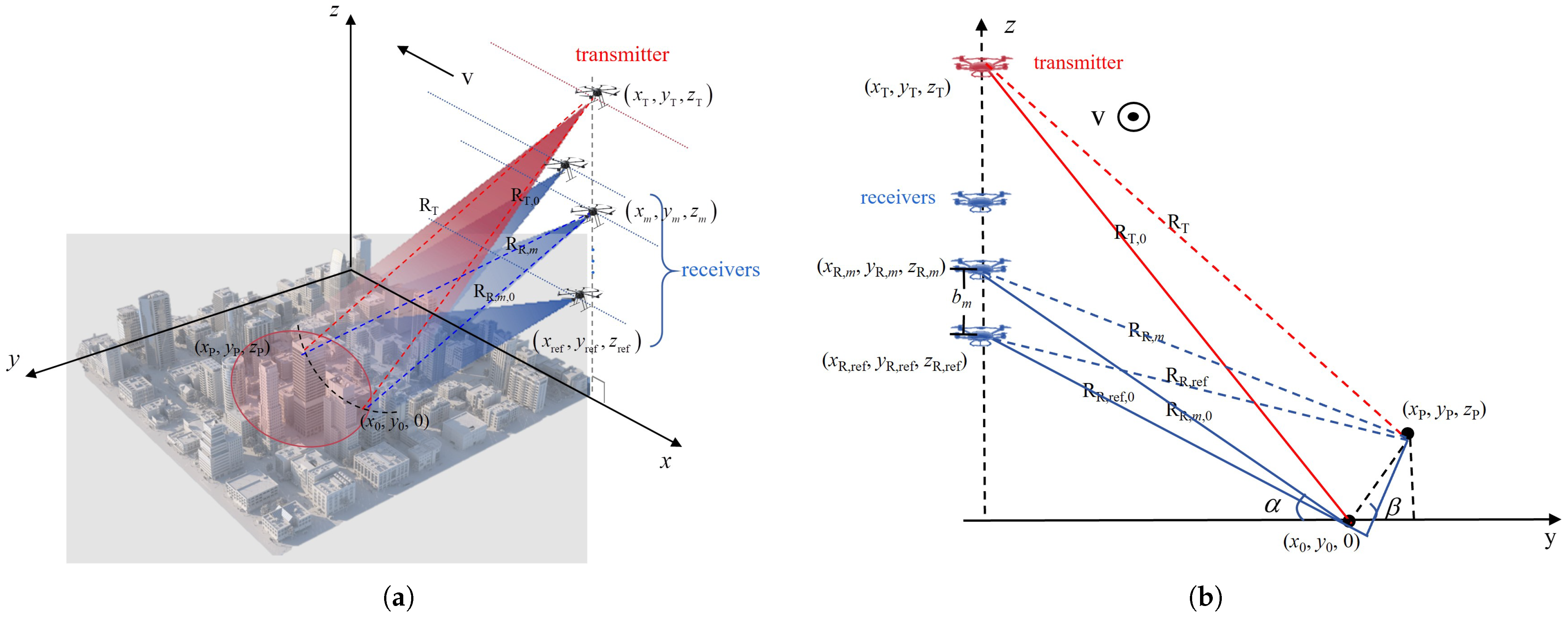
In distributed UAV TomoSAR, platform spacing must satisfy safety constraints. This requires a three-dimensionally staggered UAV arrangement, rather than using a traditional linear geometry. The system layout and cross-sectional view in a single-transmit multi-receive (STMR) mode are shown in Figure 1. In STMR mode, one primary UAV transmits pulses, while the entire swarm (M platforms) performs synchronous reception. This effectively creates M elevation sampling points, providing the spatial diversity for 3D imaging. As shown in Figure 1, the UAVs move uniformly at the same velocity along the x-axis in side-looking mode. The azimuth direction aligns with the x-axis, and the range direction projects onto the y-axis on the ground.

Figure 1. Geometric configuration of a distributed unmanned aerial vehicle (UAV) tomographic synthetic aperture radar (TomoSAR) three-dimensional (3D) system under staggered 3D spatial conditions. (a) 3D schematic view; (b) Y–z plane view.

In a distributed multi-UAV STMR TomoSAR system, azimuth misalignment and staggered 3D spatial configurations may cause different receiving channels to have inconsistent effective azimuth observation supports. To enable coherent multi-platform fusion, this paper adopts an equivalent phase-center (EPC)-based common-aperture processing strategy: for each bistatic channel, the transmitter and receiver positions are combined to form an EPC trajectory. Its azimuth coordinate is then used as a unified parameter, and a common-aperture crop is applied to all channels to obtain a shared azimuth observation interval.

Under the far-field and small-angle approximation commonly used in TomoSAR, the elevation-dependent phase term for the m-th effective baseline can be written as a Fourier-type sampling of the elevation reflectivity profile. Discretizing the elevation axis ${\left\{s_n\right\}}_{n=1}^N$, the per-channel measurement is

$$I_m=\sum _{n=1}^N{\sigma }_n{e}^{j2\pi {\xi }_m{s}_n}+{\epsilon }_m,m=1,\dots ,M.$$

(1)

where ${\sigma }_n$ is the scattering coefficient of $s_n$, ${\epsilon }_m$ is noise of the m-th receiver, ${\xi }_M$ is the spatial frequency. According to [33], ${\xi }_m=sin(\alpha +\beta )b_{m,\perp }/\left(\lambda R_{R,\mathrm{ref},0}\right)$, the definitions of $\alpha$ and $\beta$ are shown in Figure 1, $b_{m,\perp }$ denotes the elevation direction projection, $\lambda$ is the wavelength, and $R_{R,\mathrm{ref},0}$ is the reference slant range. Stacking these measurements over $m=1,\dots ,M$ forms the multi-platform observation vector:

$$\mathbf{IM}=\mathbf{A}\ast \mathit{\sigma }+\mathit{\epsilon }$$

(2)

where $\mathit{\sigma }$ is the elevation scattering coefficient vector, $\mathit{\epsilon }$ is the noise vector, and the sensing matrix $\mathbf{A}$ can be expressed as

$$\mathbf{A}=\left[\begin{array}{ccc}exp\left(j2\pi {\xi }_1{s}_1\right)& \dots & exp\left(j2\pi {\xi }_1{s}_N\right)\\ ⋮& \ddots & ⋮\\ exp\left(j2\pi {\xi }_M{s}_1\right)& \dots & exp\left(j2\pi {\xi }_M{s}_N\right)\end{array}\right]$$

(3)

It can be seen that the imaging model is essentially the same as that of conventional monostatic TomoSAR.

According to CS theory, the reconstruction performance is limited by the properties of the sensing matrix [21,22], and the sparse 3D sensing matrix of distributed UAV SAR is closely related to the system geometric configuration. Therefore, optimizing the configuration of a distributed UAV SAR system can achieve better imaging performance.

The effective baseline is the projection of the UAV platform space baseline in elevation. Consequently, optimizing the configuration is equivalent to optimizing the elevation-projected baseline distribution. The mutual correlation can be used to characterize the correlation of $\mathbf{A}$:

$${\mu }_{max}\left(\mathbf{A}\right)=\underset{1\le i<j\le N}{max}\left|⟨{\mathbf{a}}_i,{\mathbf{a}}_j⟩\right|$$

(4)

where ${\mathbf{a}}_i$ and ${\mathbf{a}}_j$ are any two distinct columns of the sensing matrix $\mathbf{A}$, and each column has been normalized. A smaller ${\mu }_{max}\left(\mathbf{A}\right)$ indicates lower redundancy among columns and is more favorable for sparse reconstruction. However, the maximum mutual correlation is a worst-case metric: it captures only the largest pairwise coherence and may not reflect overall performance. Therefore, the K-th order cumulative coherence [34] is introduced and defined as

$${\mu }_{1,K}\left(\mathbf{A}\right)=\underset{|\Omega |=K}{max}\underset{|\Phi |=N-K}{max}\sum _{j\in \Phi }\sum _{i\in \Omega }\left|⟨{\mathbf{a}}_i,{\mathbf{a}}_j⟩\right|$$

(5)

where $\Omega \subseteq \{1,2,\dots ,N\}$ is the index set under the K-sparse assumption, meaning that K columns are selected from all columns of the sensing matrix $\mathbf{A}$, and $\Phi$ denotes the complement of $\Omega$. ${\mathbf{a}}_i$ denotes the i-th column of $\mathbf{A}$ indexed by $\Omega$, and ${\mathbf{a}}_j$ denotes the j-th column of $\mathbf{A}$ indexed by $\Phi$. From the imaging mechanism perspective, the expression of the sensing matrix reflects the ambiguity function characteristics, and the sidelobe level is positively correlated with the inter-column correlation. Therefore, optimizing the platform locations improves the sampling of the elevation-projected baseline $b_{m,\perp }$, thereby reducing coherence, suppressing sidelobes, and ultimately enhancing 3D reconstruction quality.

3. Modeling of the Configuration Optimization Design Problem

3.1. Constraint Analysis

As shown in the previous section, the imaging quality of distributed UAV SAR 3D imaging is strongly correlated with the geometric configuration. However, unlike array and multi-pass modes that only need to consider baseline positions, the simultaneous operation of distributed UAVs introduces additional constraints to configuration design. This paper analyzes constraints from three aspects: 3D spatial span constraints, safety distance constraints, and mainlobe mutual-illumination avoidance constraints. Let the position of the i-th UAV be

$${\mathbf{p}}_i={[x_i,y_i,z_i]}^{\mathsf{T}},i=1,\dots ,M$$

(6)

3.1.1. The 3D Spatial Span Constraints

For the elevation direction, spatial coherence determines reconstructability, and the effective vertical baseline span determines elevation resolution. In [35], numerical simulations indicate that the spatial baseline length should not exceed one-third of the critical baseline. From the resolution perspective, CS can achieve super-resolution by several times the Rayleigh resolution, ensuring at least 2× Rayleigh resolution. Therefore, the maximum vertical baseline span constraint is

$${\displaystyle \frac{B_{\perp ,\rho }}{2}}\le \Delta B_{\perp ,max}\le {\displaystyle \frac{1}{3}}{B}_{\perp ,\mathrm{crit}}$$

(7)

where $B_{\perp ,\rho }$ is the equivalent baseline requirement for achieving the target elevation resolution; $B_{\perp ,\mathrm{crit}}$ is the critical vertical baseline [36], $B_{\perp ,\mathrm{crit}}=2R_{R,0}{B}_{\mathrm{rel}}cos\left({\theta }_{Bi}/2\right)tan\theta$, and $R_{R,0}$ is the reference slant range; $B_{\mathrm{rel}}=B/f_c$ is the relative bandwidth; ${\theta }_{Bi}$ represents the bistatic geometry-angle metric; and $\theta =\left({\theta }_1+{\theta }_2\right)/2$, ${\theta }_1$ and ${\theta }_2$ are the angles between the slant ranges from receivers 1 and 2 to the imaging center and the horizontal-plane normal, respectively.

For the range direction, far-field approximation is usually adopted in imaging-model analysis to neglect the influence of the baseline parallel component. Under the far-field assumption, the phase error introduced by the approximation should not exceed a threshold $\pi /8$; thus, the maximum range-direction span constraint can be written as

$$\Delta R_{max}\le \Delta R_{\mathrm{critical}}$$

(8)

where the maximum range-direction span $R_{\mathrm{critical}}$ is jointly determined by system parameters and the error threshold.

For the azimuth direction, to ensure resolution matching and imaging efficiency while constraining the feasible-solution space, the maximum azimuthal-span constraint is

$$\Delta y_{max}\le \Delta y_{\mathrm{critical}}$$

(9)

where $\Delta y_{\mathrm{critical}}$ denotes the maximum range span, which is selected according to practical conditions. Under the above 3D performance constraints, feasible solutions are restricted within a bounding box. Through the above 3D performance constraints, the feasible solution space is confined within a bounding box.

3.1.2. Safety Distance Constraints

Considering uncertainties such as positioning errors, control errors, and aerodynamic disturbances, an ellipsoidal safety region is used to describe the protected space of the i-th UAV:

$${(\mathbf{p}-{\mathbf{p}}_i)}^{\mathsf{T}}{\mathbf{A}}_i(\mathbf{p}-{\mathbf{p}}_i)\le 1$$

(10)

where ${\mathbf{A}}_i={\mathbf{R}}_i^{\mathsf{T}}{\mathbf{\Lambda }}_i{\mathbf{R}}_i$, ${\mathbf{R}}_i$ is the rotation matrix that determines the principal-axis directions of the ellipsoid, and ${\mathbf{\Lambda }}_i$ is the scale matrix that determines safety margins along each direction. Under the assumptions of no tilt and approximately straight-line uniform motion, it is acceptable to set ${\mathbf{R}}_i=\mathbf{I}$. The safety distance constraint between any two UAVs i and j is written as

$${({\mathbf{p}}_i-{\mathbf{p}}_j)}^{\mathsf{T}}{\mathbf{\Lambda }}_i({\mathbf{p}}_i-{\mathbf{p}}_j)\ge 1,i\ne j$$

(11)

3.1.3. Mainlobe Illumination Avoidance Constraints

To avoid front-end saturation or strong interference caused by platforms entering each other’s mainlobes, the mainlobe is approximated by a cone. For any UAV pair $(i,j)$, mutual mainlobe avoidance requires

$$\left\{\begin{array}{cc}\hfill ({\mathbf{p}}_j-{\mathbf{p}}_i)·{\mathbf{d}}_i& <\parallel {\mathbf{p}}_j-{\mathbf{p}}_i\parallel cos{\alpha }_i,\hfill \\ \hfill ({\mathbf{p}}_i-{\mathbf{p}}_j)·{\mathbf{d}}_j& <\parallel {\mathbf{p}}_i-{\mathbf{p}}_j\parallel cos{\alpha }_j.\hfill \end{array}\right.$$

(12)

where ${\mathbf{d}}_i$ is the unit vector along the mainlobe pointing direction of the i-th UAV, and ${\alpha }_i$ is its half-cone angle. The first inequality ensures that the j-th UAV stays outside the mainlobe of UAV i, whereas the second inequality enforces the reciprocal condition, i.e., UAV i stays outside the mainlobe of UAV j.

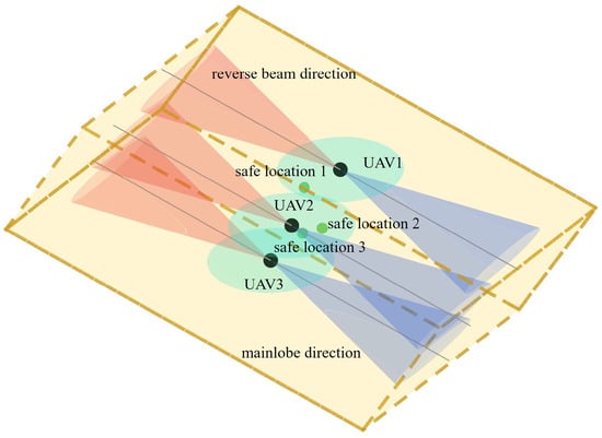
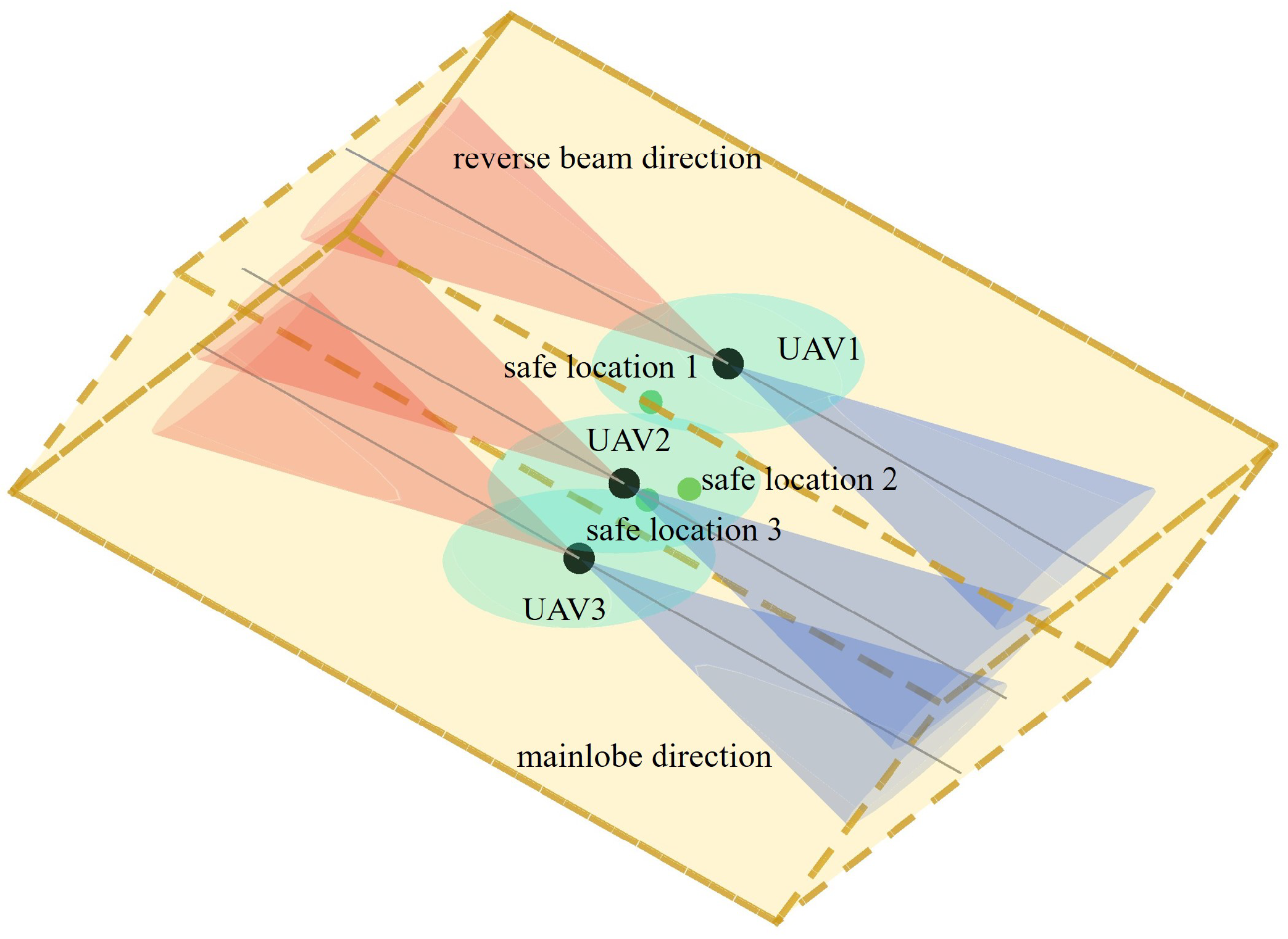
Combining the above constraints, the spatial constraints of the distributed UAV SAR 3D imaging system are modeled and presented in Figure 2, with three UAVs as the example case. The result demonstrates that under the superposition of multiple constraints, the feasible region in 3D space becomes discrete and fragmented. In the next subsection, we develop a configuration optimization model based on these composite constraints.

Figure 2. Schematic illustration of the composite constraints in the distributed UAV SAR system. Yellow box is 3D span constraint. Green ovals is safe spacing constraints. Orange and blue cone are Beam constraints.

It should be noted that this ellipsoidal safety region is designed to provide static spatial redundancy during the pre-mission planning stage, serving as a baseline for safe separation under nominal flight conditions.

3.2. Optimization Model

In distributed UAV 3D imaging configuration optimization, optimizing the sensing matrix performance is crucial for ensuring low coherence and good recoverability. To this end, the Gram matrix is introduced to describe correlations among all column pairs. With the columns of $\mathbf{A}$ normalized, its coherence is directly characterized by the off-diagonal elements of the Gram matrix:

$$\mathrm{Gram}\left(\mathbf{A}\right)={\mathbf{A}}^{\mathsf{H}}\mathbf{A},g_{ij}=⟨{\mathbf{a}}_i,{\mathbf{a}}_j⟩$$

(13)

The diagonal entries of the Gram matrix represent the self-inner products of the column vectors; after normalization, they are identically 1 and can be neglected. To mitigate the mainlobe’s leakage across multiple elevation bins, we exclude mainlobe-related cross-correlation terms from the correlation computation. Under low signal-to-noise-ratio (SNR) conditions, we down-weight bins near the mainlobe to improve robustness. Therefore, the sensing matrix optimization problem is modeled as follows: with the 3D coordinates of the distributed UAV swarm as decision variables, minimize the K-th order cumulative coherence of the sensing matrix. The baseline optimization problem can be modeled as

$$f_{\mathrm{correlation}}\left(\mathbf{P}\right)=min{\mu }_{1,K}\left(\mathbf{A}\right)$$

(14)

By solving this model, the optimal baselines can be obtained. In addition, according to the previous analysis, the 3D bounding-box constraints only provide the upper bounds of the spatial spans, and the bounding box should be made as small as possible. Therefore, while ensuring favorable effective-baseline performance in the elevation direction, a compactness metric should also be introduced. By weighted aggregation of spans along the three dimensions, the spatial compactness metric of the distributed SAR system is

$$f_{\mathrm{compact}}\left(\mathbf{P}\right)=min\left(w_R\Delta R_{max}+w_y\Delta y_{max}+w_B\Delta B_{\perp ,max}\right)$$

(15)

where $w_R$, $w_y$ and $w_B$ are the weights for corresponding dimensions. Since the impacts of the three dimensions differ, the weights can be adjusted according to the geometric configuration and mission requirements. Meanwhile, since optimizing sensing matrix performance is the primary objective and the compactness metric is secondary, it can also be written in a weighted form. Integrating the objectives and constraints, the overall configuration optimization problem of distributed UAV SAR 3D imaging is formulated as follows:

$$\begin{array}{cc}\hfill min& \underset{|\Omega |=K}{max}\underset{|\Phi |=N-K}{max}\sum _{j\in \Phi }\sum _{i\in \Omega }{w}_{ij}{g}_{ij}+w_1\left(w_R\Delta R_{max}+w_y\Delta y_{max}+w_B\Delta B_{\perp ,max}\right)\hfill \\ \hfill \mathrm{s}.\mathrm{t}.& \mathrm{C}1:|i-j|>{\displaystyle \frac{L-1}{2}},\hfill \\ \hfill & \mathrm{C}2:w_{ij}=\left\{\begin{array}{cc}1,\hfill & |i-j|-{\displaystyle \frac{L-1}{2}}>N_{tl},\hfill \\ w_{\mathrm{SNR}},\hfill & |i-j|-{\displaystyle \frac{L-1}{2}}\le N_{tl},\hfill \end{array}\right.\hfill \\ \hfill & \mathrm{C}3:{\displaystyle \frac{B_{\perp ,\rho }}{2}}\le \Delta B_{\perp ,max}\le {\displaystyle \frac{B_{\perp ,\mathrm{crit}}}{3}},\hfill \\ \hfill & \mathrm{C}4:\Delta R_{max}\le \Delta R_{\mathrm{critical}},\hfill \\ \hfill & \mathrm{C}5:\Delta y_{max}\le \Delta y_{\mathrm{critical}},\hfill \\ \hfill & \mathrm{C}6:{({\mathbf{p}}_i-{\mathbf{p}}_j)}^{\mathsf{T}}{\mathbf{\Lambda }}_i({\mathbf{p}}_i-{\mathbf{p}}_j)\ge 1,\forall i\ne j,\hfill \\ \hfill & \mathrm{C}7:({\mathbf{p}}_j-{\mathbf{p}}_i)·{\mathbf{d}}_i<\parallel {\mathbf{p}}_j-{\mathbf{p}}_i\parallel cos{\alpha }_i,\forall i\ne j.\hfill \end{array}$$

(16)

where L is the number of oblique diagonal lines covered by the mainlobe; $w_{ij}$ is the weight; $g_{ij}$ is the $(i,j)$ element of the Gram matrix; and $w_1$ denotes the weight of Objective 2.

Under normal circumstances, the cumulative coherence value is in the range $[0,K]$, while the compactness index range is determined by the constraint space and usually not in the same order of magnitude. To ensure the optimization process is primarily driven by imaging performance and treat the secondary objective compactness as a regularization term, the two indicators should be maintained in similar numerical ranges through the setting of $w_1$, with adjustments made according to practical conditions.

The settings of $w_R$, $w_y$, $w_B$ are mainly determined by the task and scenario. For example, when flying in narrow valleys, $w_R$ and $w_y$ need to be strengthened; a higher pursuit of coherence requires strengthening $w_B$; and a higher pursuit of height resolution requires weakening $w_B$. $w_{\mathrm{SNR}}$ is mainly adjusted based on the SNR. Under low-SNR conditions, this value should be minimized to trade slight position deviations for reduced coherence. Under high-SNR conditions, this value can be increased to achieve precise position reconstruction as much as possible.

4. Configuration Optimization Method

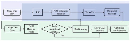
Distributed UAV SAR configuration optimization involves both imaging performance and multiple constraints, leading to a fragmented feasible region and high dimensionality. Direct global search in the 3D position space is inefficient. Therefore, this paper adopts a “two-stage dimensionality-reduction” hierarchical recursive strategy: Stage 1 obtains a near-global performance-optimal solution in the baseline domain, and Stage 2 explicitly incorporates constraints in the spatial domain and constructs a compact configuration via recursive analytical synthesis.

(1)

Stage 1: Global baseline optimization

With a fixed elevation grid, the sensing matrix performance is mainly determined by the effective baseline distribution; thus, Stage 1 performs global optimization using only baseline vectors as decision variables, which significantly reduces the search dimension. PSO employs a socially guided velocity update mechanism that offers a distinct advantage in initial descent speed [37]. Meanwhile, CMA-ES demonstrates superior optimization potential by adaptively learning the covariance structure of the search space [38,39]. Consequently, to balance global exploration and local convergence, the hybrid combination of these two methods enables both faster and higher-quality performance optimization. Specifically, PSO is used for coarse search [37], and after the improvement-rate threshold is met, the method switches to CMA-ES for refined optimization. To adapt to different parameter settings, a relative improvement rate is introduced as the dynamic switching criterion:

$${\Delta }_k={\displaystyle \frac{f\left(g_{\mathrm{best}}^{(k-L)}\right)-f\left(g_{\mathrm{best}}^{\left(k\right)}\right)}{\left|f\left(g_{\mathrm{best}}^{(k-L)}\right)\right|+\delta }}$$

(17)

where $f(·)={\mu }_{1,K}(·)$ denotes the objective-function value in this paper, namely the K-th order cumulative coherence, $g_{\mathrm{best}}^{\left(k\right)}$ is the global best value at iteration k, and $\delta$ is a small constant. This criterion uses a sliding window to evaluate the improvement rate of the current optimization result relative to the best value over the past L generations. The specific steps of the hybrid PSO–CMA-ES are shown as Table 1.

Table 1. Procedure of the hybrid PSO-CMA-ES.

Stage 1	Global Baseline Optimization
1	Initialize PSO parameter: population size D, maximum number of iterations $K_{max}$ strategy switching threshold $K_{switch}$ and ${\epsilon }_{switch}$;
2	Update particle velocity $v_{i,m}^{(k+1)}$ and position ${\mathbf{b}}_{i,\perp }^{(k+1)}$;
3	Compute fitness $f_i={\mu }_{1,K}\left(\mathbf{A}\left({\mathbf{b}}_i^{(k+1)}\right)\right)$, update personal best ${\mathbf{p}}_{\mathrm{best},i}^{(k+1)}$ and global best $g_{\mathrm{best}}^{(k+1)}$;
4	Terminate PSO if the iteration count reaches $K_{switch}$ or the relative improvement rate is below ${\epsilon }_{switch}$ for L consecutive generations; otherwise, return to Step 2;
5	Initialize CMA-ES parameters: use the best baseline obtained by PSO as the initial distribution mean ${\mathbf{m}}^{\left(0\right)}={\mathbf{b}}_{\mathrm{pso}}$, initialize step size ${\sigma }^{\left(0\right)}=UB\ast {10}^{-3}$, initialize covariance matrix ${\mathbf{C}}^{\left(0\right)}=\mathbf{I}$;
6	Sample $\lambda$ candidate solutions: ${\mathbf{b}}_i^{\left(k\right)}\sim \mathcal{N}\left({\mathbf{m}}^{\left(k\right)},{\sigma }^{\left(k\right)}{)}^2{\mathbf{C}}^{\left(k\right)}\right)$ evaluate fitness, and select the best $\mu$ solutions;
7	Update the distribution mean ${\mathbf{m}}^{\left(t\right)}$ of the best $\mu$ solutions, conjugate evolution path ${\mathbf{p}}_{\sigma }$, covariance evolution path ${\mathbf{p}}_c$, covariance matrix ${\mathbf{C}}^{(k+1)}$, and global step size ${\sigma }^{\left(t\right)}$;
8	Terminate CMA-ES if the iteration count reaches $K_{max}$ or the step size is below ${\epsilon }_{\sigma }$, and output ${\mathbf{B}}^{*}=\{b_1^{*},b_2^{*},\dots ,b_{M-1}^{*}\}$; otherwise, return to Step 6.

(2)

Stage 2: Recursive optimization of spatial configuration sequence

In the second stage, after obtaining the globally optimal baseline set, an anchor point is fixed and, under engineering constraints, the elevation–direction baselines are mapped back to specific 3D coordinates $\mathbf{P}=\{{\mathbf{p}}_1,{\mathbf{p}}_2,\dots ,{\mathbf{p}}_M\}$, while improving system compactness as much as possible. After the Stage 1 baseline optimization, each UAV position is constrained to a specific slant-range plane determined by the imaging geometry, thereby reducing the 3D problem dimension. Then, with a reference UAV selected as the initial anchor, a near-to-far topological expansion strategy is adopted to recursively determine, in sequence, the compactness-optimal locations of adjacent nodes within the feasible region. For maximizing search redundancy and improving system compactness, the geometric center of the envelope can be selected as the initial anchor. The feasible region is obtained analytically by excluding areas that violate constraints such as safety separation and mutual beam illumination. If infeasibility occurs or the solution becomes trapped in a local optimum, the recursion continues after backtracking to adjust previously determined nodes. Ultimately, a compact distributed UAV 3D imaging configuration that satisfies all constraints is obtained. The specific steps of Stage 2 are shown as Table 2.

Table 2. Procedure of the recursive optimization.

Stage 2	Recursive Spatial Configuration
1	Select a reference UAV as the anchor and initialize its 3D coordinates ${\mathbf{P}}_{\mathrm{ref}}={[0,0,H_{\mathrm{ref}}]}^{\mathsf{T}}$;
2	Sort the remaining UAVs by baseline magnitude to form the recursive optimization sequence $\mathcal{Q}=\{q_1,q_2,\dots ,q_M\}$;
3	Construct the baseline-constraint plane ${\mathcal{S}}_k$ 1 for the k-th UAV in the optimization sequence according to the SAR imaging geometry;
4	Remove regions violating constraints on the baseline plane ${\mathcal{S}}_k$ and prune to obtain the feasible region ${\Omega }_k$ 2;
5	Traverse the feasible region within ${\Omega }_k$ using system compactness optimality as the criterion, and solve the optimal position analytically.
6	Terminate the current recursion when the feasible region ${\Omega }_k$ is empty and activates the backtracking and quadrant-jump mechanisms:
	6.1 Divide the baseline plane of the preceding node $k-1$ into four quadrants (based on azimuth and range directions), centered on its current position. 6.2 Mark the quadrant space currently occupied by the preceding node $k-1$ as a “taboo state,” and the optimization index is then rolled back to node $k-1$. 6.3 Constrain the solution space for node to the remaining, non-taboo quadrants to find a new feasible solution. If no solution is found after traversing all quadrants at this level, the backtracking process continues recursively. 6.4 If backtracking to the anchor still cannot find a feasible solution or the total number of global backtracks exceeds the threshold $N_{\mathrm{Back}}$, return to Stage 1 for re-optimization.
7	Terminates and outputs the optimal 3D configuration coordinate set ${\mathbf{P}}^{*}=\{{\mathbf{p}}_1^{*},{\mathbf{p}}_2^{*},\dots ,{\mathbf{p}}_M^{*}\}$ satisfying all constraints if the iteration count reaches M; otherwise, return to Step 2.

¹${\mathcal{S}}_k:z_k=z_{\mathrm{ref}}+b_k^{*}/sin{\theta }_{\mathrm{inc}}-(y_k-y_{\mathrm{ref}})cot{\theta }_{\mathrm{inc}}$, ${\theta }_{\mathrm{inc}}$ is the central incidence angle; ² ${\Omega }_k={\mathcal{S}}_k\cap {\left({\bigcap }_{j\in {\mathcal{U}}_{\mathrm{fixed}}}{\mathcal{C}}_{\mathrm{safe}}\left({\mathbf{p}}_j\right)\right)}^c\cap {\left({\bigcap }_{j\in {\mathcal{U}}_{\mathrm{fixed}}}{\mathcal{C}}_{\mathrm{beam}}\left({\mathbf{p}}_j\right)\right)}^c\cap {\mathcal{R}}_{\mathrm{box}}$, ${\mathcal{U}}_{\mathrm{fixed}}$ is the set of fixed nodes, ${\mathcal{C}}_{\mathrm{safe}}\left({\mathbf{p}}_j\right)$ is the projection region on of safety ellipsoids generated by fixed nodes j, ${\mathcal{C}}_{\mathrm{beam}}\left({\mathbf{p}}_j\right)$ is the projection region of the dual-cone mainlobe constraint, ${\mathcal{R}}_{\mathrm{box}}$ is the system performance envelope constraint region.

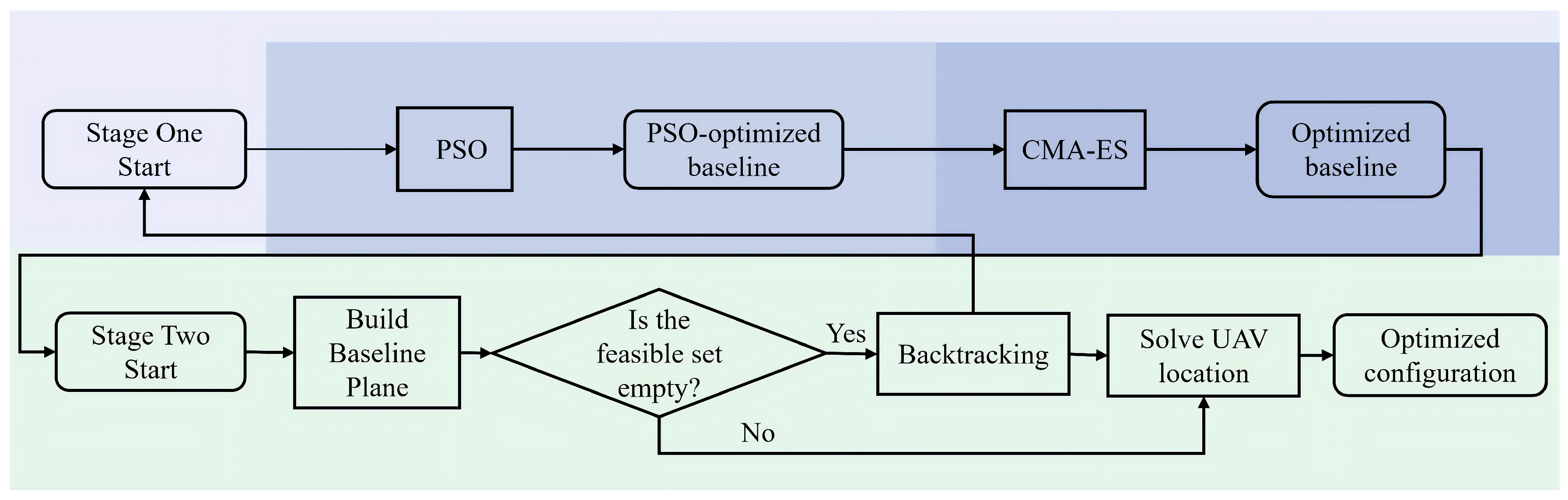
The algorithm flowchart is shown in Figure 3.

Figure 3. Algorithm flowchart.

5. Experimental Results

This section validates the effectiveness of the proposed configuration optimization design method for distributed UAV TomoSAR 3D imaging through simulations. We first present an azimuth–elevation profile simulation using a 2D slice target, comparing the imaging results between a randomly generated configuration (which still satisfies all constraints) and the optimized configuration. This comparison includes the magnitude maps of the normalized sensing-matrix Gram matrix as well as the final reconstruction results. Subsequently, we perform 3D imaging of a complex building target for further validation. The system parameters are listed in Table 3. The sparsity order in the cumulative coherence is set to 3, following the common observation in urban TomoSAR that a single resolution cell typically contains no more than three dominant scatterers [20]. The algorithm switch threshold of Stage 1 is 0.03 according to PSO convergence. To prevent CMA-ES updates from jumping out of the high-quality solution region identified by PSO, the initial step size for CMA-ES is set to 0.001, which is significantly smaller than the common starting step sizes typically used in standard implementations.

Table 3. Simulation system parameters for configuration optimization design.

Parameter	Value
Carrier frequency	9.5 GHz
Range sampling bandwidth	500 MHz
Reference range	5 km
Number of UAVs	16
Maximum azimuth spans	100 m
Maximum range spans	100 m
Maximum elevation spans	100 m
Safety azimuth separation	20 m
Safety range separation	15 m
Safety elevation separation	10 m

Under the system settings of this paper, the optimized cumulative coherence is approximately 1, and the order of magnitude of the compactness index typically ranges from $\mathcal{O}\left({10}^2\right)$ to $\mathcal{O}\left({10}^3\right)$. To match their orders of magnitude and ensure the coherence of the measurement matrix is the primary optimization objective, $w_1=1\times {10}^{-4}$. Additionally, since this paper does not impose special task or terrain requirements, we set $w_R=1,w_y=1,w_B=1$, a balanced weight distribution that yields the most robust results. Meanwhile, to sufficiently suppress coherence, this paper sets $w_{SNR}=0$.

Assuming that the transmitter and the receiver swarm are in close proximity, the bistatic angle is neglected. According to the critical baseline formula, the upper bound of the elevation baseline is 289 m, and according to the elevation resolution formula, the lower bound is 75 m; thus, the maximum elevation span is set to 100 m in this paper. Using a phase error of $\pi /8$ as the threshold for the far-field approximation, the maximum range span is 178 m, and 100 m is adopted in this paper. The azimuth span is set as small as possible, and 100 m is also used in this paper.

5.1. 2D Slice Target

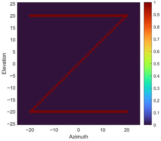
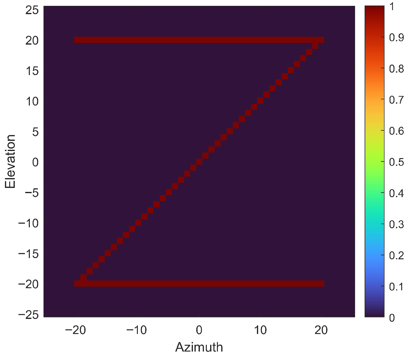
This subsection observes the effect via the azimuth–elevation profile. To intuitively verify the advantages of the proposed configuration optimization algorithm in suppressing imaging sidelobes and improving sparse reconstruction accuracy, a “Z”-shaped lattice target is used for simulation analysis, as shown in Figure 4.

Figure 4. Simulation target letter Z.

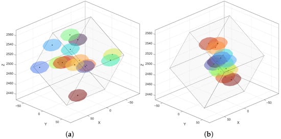
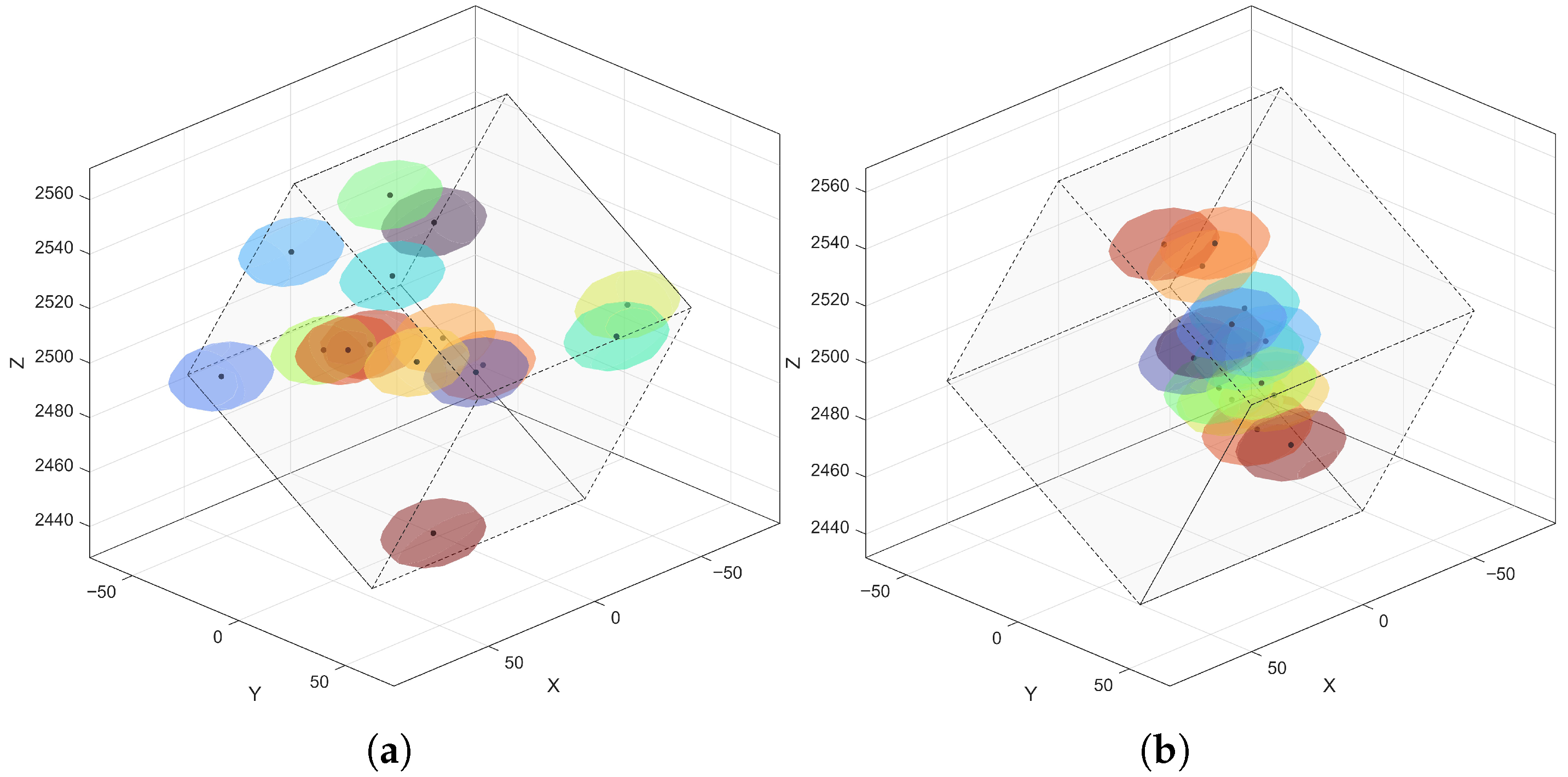
Based on the target profile, the elevation grid range is set to 50 m with 101 grid points. Under this condition, the 3D configurations of the distributed UAVs for random placement and optimized placement are shown in Figure 5. To more clearly show the configuration distribution, the figure displays only the 3D performance constraint bounding box and the safety distance constraints.

Figure 5. Three-dimensional configuration of the distributed UAV SAR system. (a) Random configuration; (b) optimized configuration. Ellipsoids of different colors represent the safe spacing for different UAVs.

Visually, to satisfy the constraints, UAVs in the random configuration are scattered in space, while UAVs in the optimized configuration have obviously higher compactness, because the recursive strategy can sensitively capture positions that satisfy compactness. The final optimization costs for the random and optimized configurations are 2.14 and 0.91, respectively. Due to the compactness constraint, in the X and Y dimensions, UAVs should be distributed as much as possible around the center.

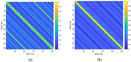
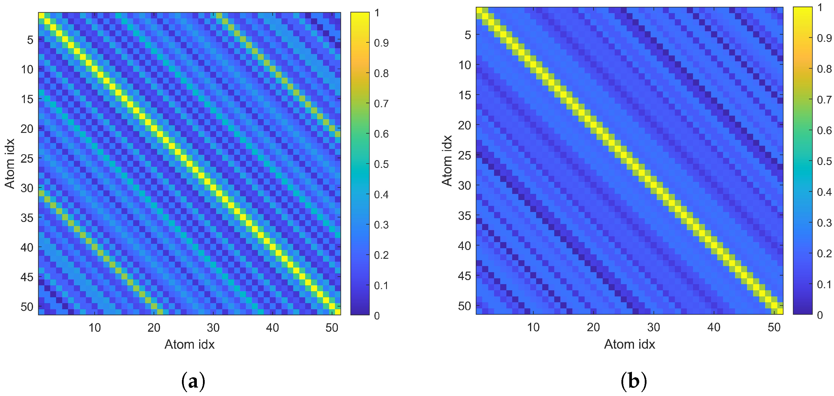
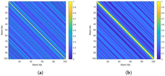
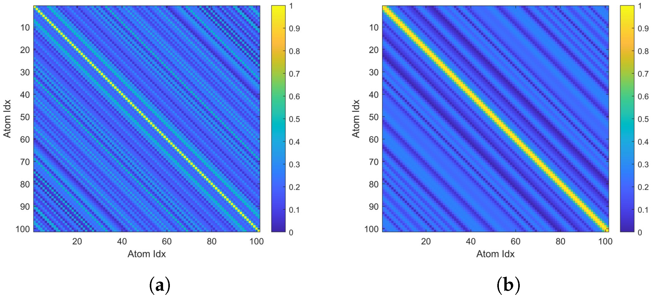
The off-diagonal elements of the Gram matrix characterize the cross-correlation between columns of the sensing matrix. The Gram matrices under the two configurations are shown in Figure 6.

Figure 6. Comparison of Gram matrices for target letter Z. (a) Random configuration; (b) Optimized configuration.

From Figure 6a, the Gram matrix of the random configuration shows high redundancy among observation data at different elevation grids, which can easily cause confusion in support recovery for CS algorithms. In contrast, in Figure 6b, the off-diagonal energy of the Gram matrix under the optimized configuration is significantly reduced, showing good near-diagonalization. This indicates that after configuration optimization using the proposed method, the cross-correlation of the sensing matrix is substantially reduced. The computed third-order cumulative coherence values under the random and optimized configurations are 1.67 and 0.83, respectively.

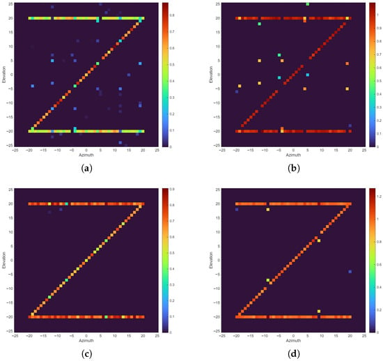
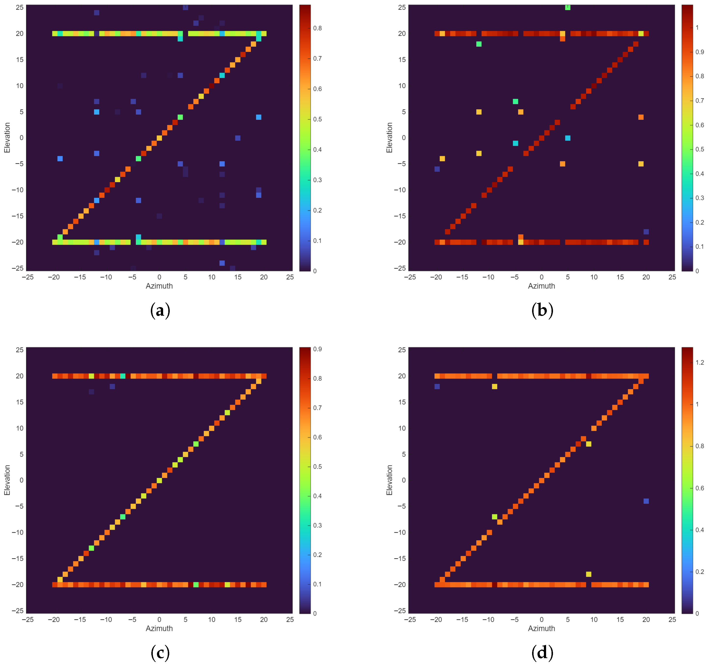
Using the Iterative Shrinkage Thresholding Algorithm (ISTA) [40] and Orthogonal Matching Pursuit (OMP) [41] algorithm, the reconstruction results of the letter “Z” under the random and optimized configurations are shown in Figure 7. To evaluate the robustness of the proposed configuration optimization method under realistic conditions, complex additive white Gaussian noise is added to the simulated echo data, resulting in an SNR of 10 dB for all experiments.

Figure 7. Reconstruction results of the letter “Z”. (a) ISTA + random configuration; (b) OMP + random configuration; (c) ISTA + optimized configuration; (d) OMP + optimized configuration. The color bar indicates the reconstruction amplitude.

From the profile imaging results, both algorithms perform significantly better under the optimized configuration than under the random configuration. Under the random configuration, due to high sidelobes, the reconstruction results of ISTA and OMP exhibit a large number of scattered noise points around the “Z”-shaped target. Under the optimized configuration, the ISTA result shows a clean background and a well-defined target with almost no residual artifacts, although the amplitudes of a few true target points are attenuated. The OMP result achieves amplitudes closer to the ground truth, with a one-to-two-pixel shift at a few locations.

Peak signal-to-noise ratio (PSNR) and structural similarity (SSIM) are further introduced to quantitatively evaluate imaging quality. A larger PSNR indicates the imaging result is closer to the ground truth. SSIM closer to 1 indicates higher similarity between two images. The PSNR and SSIM values for the letter “Z” under the random and optimized configurations are shown in Table 4.

Table 4. Reconstruction quality metrics for the “Z” target.

Imaging Algorithms	Imaging Configuration	PSNR (dB)	SSIM
ISTA	Random configuration Optimized configuration	17.8 24.2	0.775 0.936
OMP	Random configuration Optimized configuration	20.9 26.2	0.797 0.965

As shown in Table 4, the optimized configuration consistently improves both PSNR and SSIM across all reconstruction algorithms. Compared with the random configuration, the PSNR increases by 6.4 dB and the SSIM increases by 0.161 when using ISTA for imaging; the PSNR increases by 5.3 dB and the SSIM increases by 0.168 when using OMP for imaging. For both algorithms, the optimized configuration achieves better performance. Next, simulations on a 3D solid target are conducted to further validate the effectiveness of the proposed method.

5.2. 3D Target

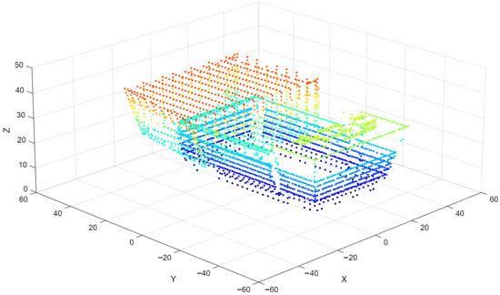
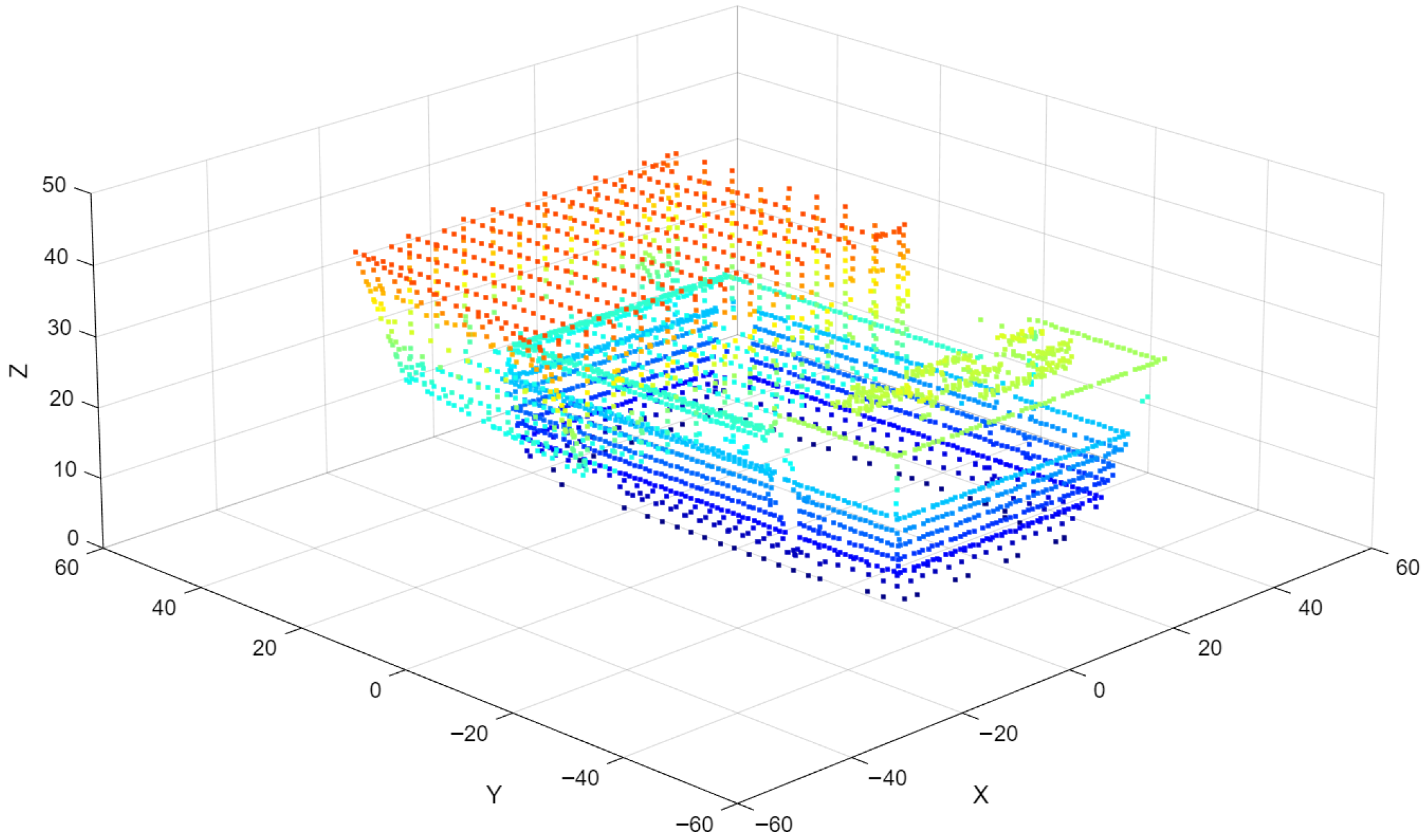
To verify effectiveness in continuous complex scenes, this subsection performs 3D reconstruction analysis for a library building target; the point cloud read from its OBJ file is shown in Figure 8.

Figure 8. Simulation target library. Different colors represent target points at different heights.

Due to the mechanism of TomoSAR imaging, although the building height is only about 40 m, the required elevation grid must be larger than the height. Therefore, for this 3D simulation target, the grid height is set to 100 m, and the number of points remains 101. The resulting Gram matrices under this condition are provided in Figure 9.

Figure 9. Comparison of Gram matrices for target library. (a) Random configuration; (b) optimized configuration.

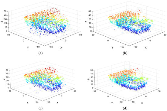
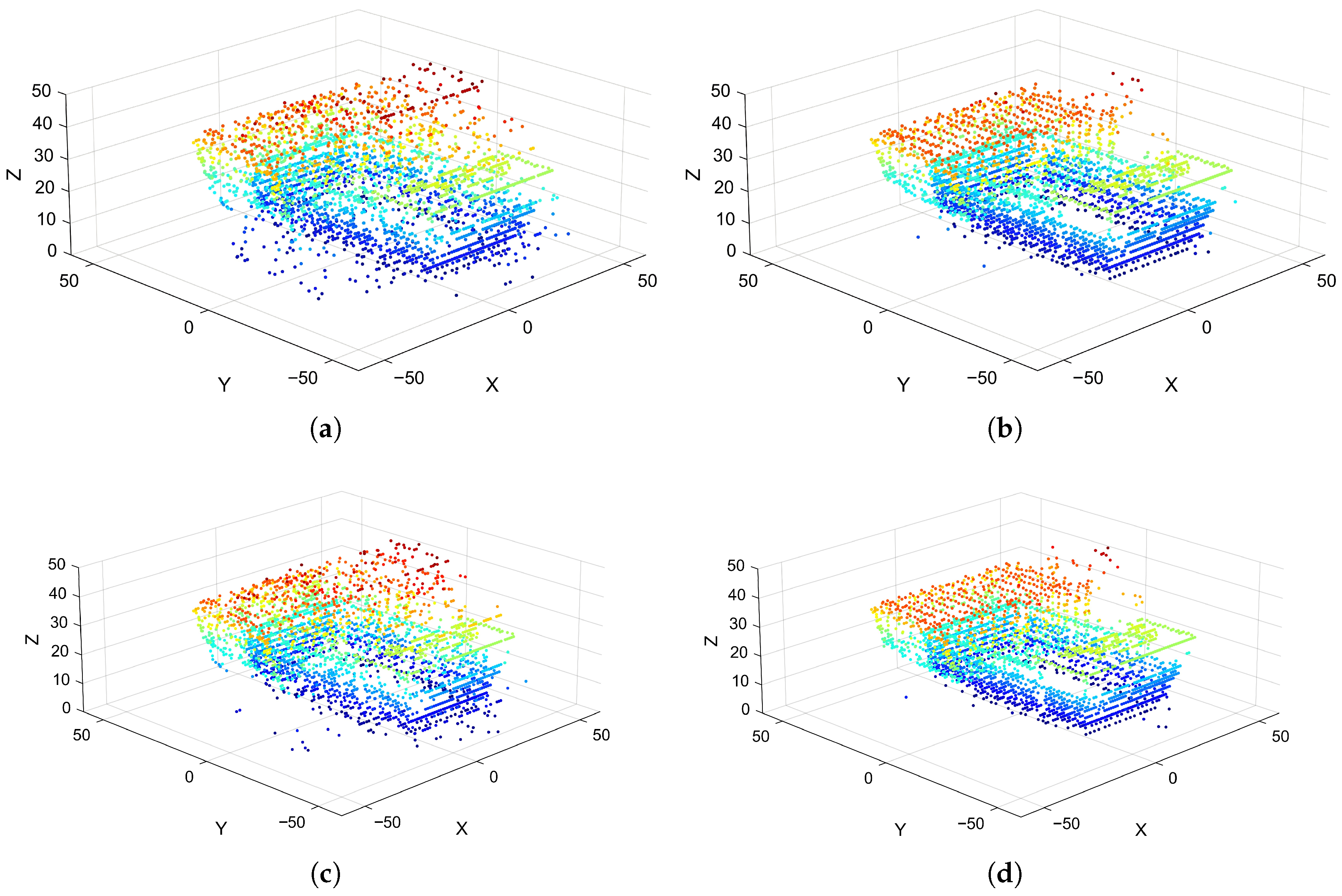
Under the optimized configuration for the 3D target, the third-order cumulative coherence value and the final optimization cost are 0.87 and 0.82, respectively. Under the random configuration used for comparison, the third-order cumulative coherence value and the final optimization cost are 1.55 and 1.45, respectively. The 3D imaging results under the two configurations are shown in Figure 10.

Figure 10. Reconstruction results for the library from a 3D perspective. (a) ISTA + random configuration; (b) ISTA + optimized configuration; (c) OMP + random configuration; (d) OMP + optimized configuration.

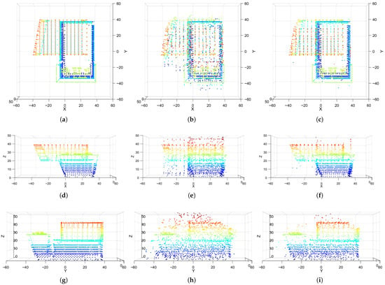
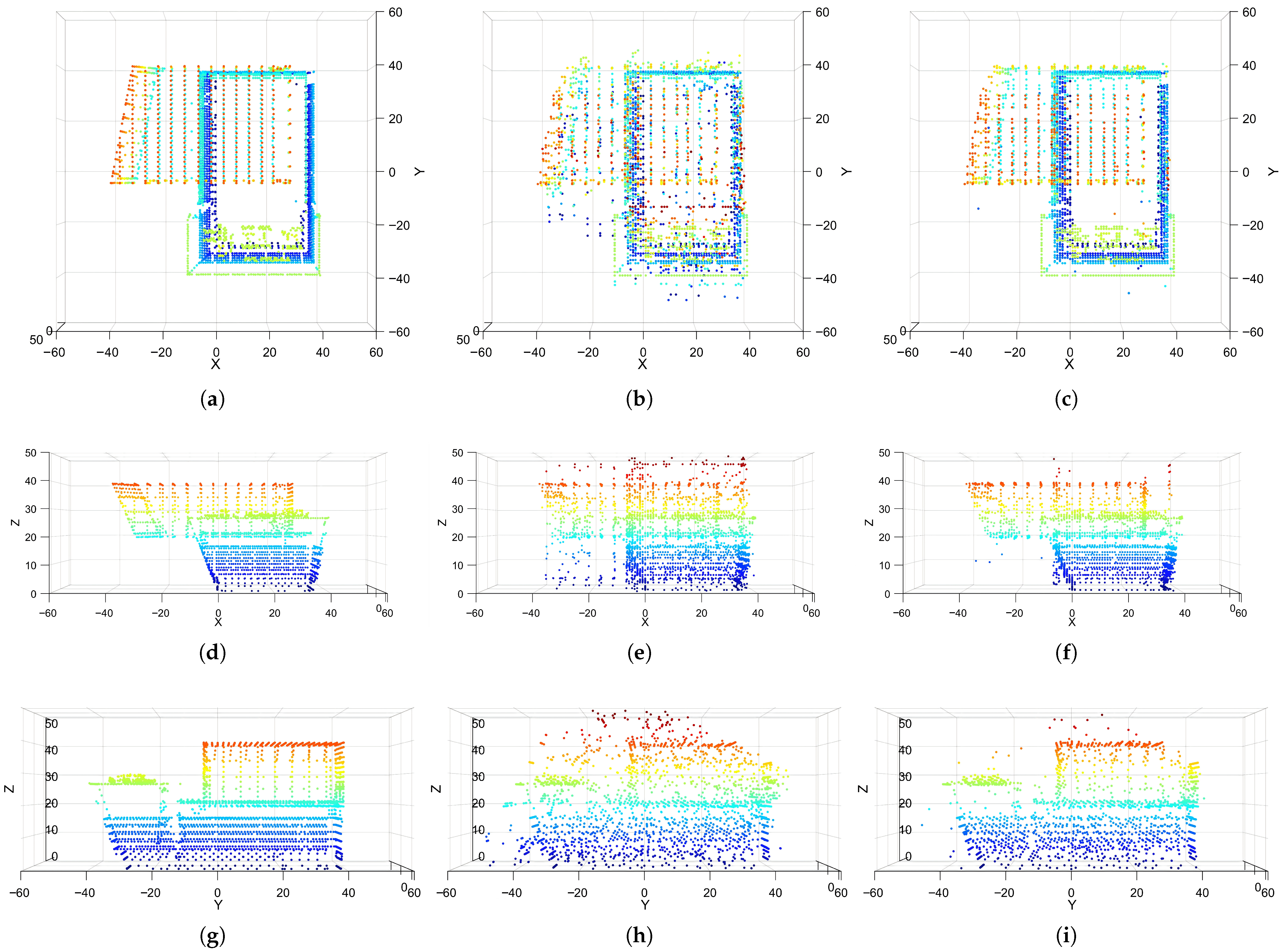
It can be seen that imaging under the optimized configuration is closer to the reference result, while imaging under the random configuration is more cluttered. The differences between the two configurations are further compared from three-view perspectives, as shown in Figure 11. As the consistent superiority of the optimized configuration over both ISTA and OMP has been established in the 3D case, this section prioritizes the results from the 2D perspective for ISTA to maintain conciseness while providing representative visual results for OMP.

Figure 11. ISTA reconstruction results for the library from a 2D perspective. (a) X-Y + Ground truth; (b) X-Y + random configuration; (c) X-Y + optimized configuration; (d) X-Z + ground truth; (e) X-Z + random configuration; (f) X-Z + optimized configuration; (g) Y-Z + ground truth; (h) Y-Z + random configuration; (i) Y-Z + optimized configuration.

From the point-cloud reconstruction results, the configuration significantly affects reconstruction quality for complex geometries: under the random configuration, wall surfaces and roof edges are blurred and contain more noise points, which can interfere with subsequent recognition and measurement. The optimized configuration significantly improves wall flatness and edge clarity, with fewer noise points. Quantitative metrics are further used to evaluate the improvement.

To quantitatively evaluate the quality of 3D point-cloud reconstruction, reconstruction accuracy and reconstruction completeness are adopted as evaluation metrics. Let the reference point cloud be ${\mathbf{PC}}_{pre}=\{p{c}_1,p{c}_2,\dots ,p{c}_{w_p},\dots ,p{c}_{W_p}\}$, where $p{c}_{w_p}=(x_{w_p},y_{w_p},z_{w_p})$ denotes the $w_p$-th point and $W_p$ is the number of points in ${\mathbf{PC}}_{pre}$$(w_p=1,\dots ,W_p)$. Similarly, define the reconstructed point cloud as ${\mathbf{PC}}_{img}=\{p{c}_1,p{c}_2,\dots ,p{c}_{w_i},\dots ,p{c}_{W_i}\}$, where $p{c}_{w_i}=(x_{w_i},y_{w_i},z_{w_i})$ and $W_i$ denotes the number of points in ${\mathbf{PC}}_{img}$$(w_i=1,\dots ,W_i)$. Reconstruction accuracy and completeness are computed as

$$\mathrm{Acc}={\displaystyle \frac{1}{W_p}}\sum _{w_p=1}^{W_p}\underset{1\le w_i\le W_i}{min}\mathrm{dist}\left({\mathbf{PC}}_{pre}\left(w_p\right),{\mathbf{PC}}_{img}\left(w_i\right)\right)$$

(18)

$$\mathrm{Com}={\displaystyle \frac{1}{W_i}}\sum _{w_i=1}^{W_i}\underset{1\le w_p\le W_p}{min}\mathrm{dist}\left({\mathbf{PC}}_{img}\left(w_i\right),{\mathbf{PC}}_{pre}\left(w_p\right)\right)$$

(19)

where $\mathrm{dist}\left({\mathbf{PC}}_{pre}\left(w_p\right),{\mathbf{PC}}_{img}\left(w_i\right)\right)$ denotes the Euclidean distance between the $w_p$-th point in ${\mathbf{PC}}_{pre}$ and the $w_i$-th point in ${\mathbf{PC}}_{img}$. In Equations (18) and (19), both metrics compute the mean nearest neighbor distance between point clouds. Accuracy measures the proximity of the reconstructed points to the reference in Equation (18), namely redundancy error, while completeness measures how well the reference is covered by the reconstruction in Equation (19), namely omission error. Lower values indicate better performance for both metrics.

According to the results in Table 5, the imaging metrics improve under both the 3D view and the 2D views. Taking the average PSNR and SSIM over the three views, the random configuration yields a mean PSNR of 13.5 dB and a mean SSIM of 0.498, whereas the optimized configuration yields a mean PSNR of 14.8 dB and a mean SSIM of 0.635. Reconstruction accuracy improves from 5.84 m to 3.39 m, indicating a better fit between the reconstructed point cloud and the true model with smaller position errors; reconstruction completeness improves from 1.04 m to 0.76 m, indicating that the reconstructed point cloud under the optimized configuration captures more true details.

Table 5. Comparison of metrics for library reconstruction under different configurations.

Imaging Views	Imaging Configuration	PSNR (dB)	SSIM	Reconstruction Accuracy	Reconstruction Completeness
3D(OMP)	Random configuration Optimized configuration	\ \	\ \	5.36 3.41	1.07 0.82
3D(ISTA)	Random configuration Optimized configuration	\ \	\ \	5.84 3.39	1.04 0.76
X-Y(ISTA)	Random configuration Optimized configuration	14.7 15.7	0.576 0.691	\ \	\ \
X-Z(ISTA)	Random configuration Optimized configuration	13.0 14.4	0.483 0.644	\ \	\ \
Y-Z(ISTA)	Random configuration Optimized configuration	12.7 14.4	0.435 0.570	\ \	\ \

6. Discussion

This section presents a further analysis of the proposed algorithm, including its performance comparison with the direct 3D optimization method and an investigation into the impacts of iteration numbers, position perturbations, and the number of UAVs.

6.1. Algorithm Performance Comparison

Due to engineering constraints such as safety separation and mainlobe mutual illumination avoidance, the feasible set in the 3D position space is highly nonconvex and fragmented into multiple disconnected regions. As a result, direct global search in the original 3D space yields a very low effective sampling rate, which severely impedes optimization. Typical heuristic algorithms, including Differential Evolution (DE) [42], Particle Swarm Optimization (PSO) [43], and Simulated Annealing (SA) [44], rely on distinct search mechanisms: DE utilizes differential mutation and crossover, PSO operates through socially guided position and velocity updates, and SA employs probabilistic acceptance of neighborhood solutions. However, when the feasible volume is extremely small and highly dispersed, randomly generated candidates frequently fall outside the feasible set. Consequently, substantial computational effort is spent on penalty evaluation, solution repair, or rejection sampling, often leading to stagnation and premature convergence. In this regime, performance is dominated by constraint handling schemes and parameter tuning, which hinders a fair assessment of the algorithms’ intrinsic optimization capability.

Based on these considerations, we adopt CMA-ES and its restart variant IPOP-CMA-ES [39] as baseline methods for comparison. CMA-ES updates the search distribution via maximum likelihood estimation, adaptively increases the sampling density around promising regions, and learns the covariance structure among variables during iterations. This enables efficient and stable search under strong coupling, scale mismatch, and narrow feasible corridors. IPOP-CMA-ES further enhances global exploration through restarts. Meanwhile, the proposed decoupled recursive optimization framework explicitly constructs and prunes the feasible set in the second stage and incorporates a backtracking mechanism to ensure feasibility and system compactness, making it better suited to problems with fragmented feasible sets.

Through 128 Monte Carlo simulations, the proposed hierarchical recursive strategy is compared with CMA-ES and IPOP-CMA-ES; the mean and variance of optimization time and results are summarized in Table 6.

Table 6. Numerical comparison table of the recursive strategy and direct 3D optimization.

Data	Mean Time	Time Standard Deviation	Mean Result	Result Standard Deviation
CMA-ES [38]	38.22 s	0.21 s	0.99	0.06
IPOP-CMA-ES [39]	56.47 s	7.65 s	0.96	0.07
The proposed algorithm	25.18 s	0.32 s	0.93	0.06

The results show that the hierarchical recursion is better in both speed and performance; it reduces 3D position iteration to 1D baseline optimization, and the space configuration recursion stage is an analytical recursion with negligible computational cost. Meanwhile, constraints are handled in stages, avoiding local optima caused by fragmented feasible regions and yielding solutions closer to the global optimum.

6.2. Influence of Iterations

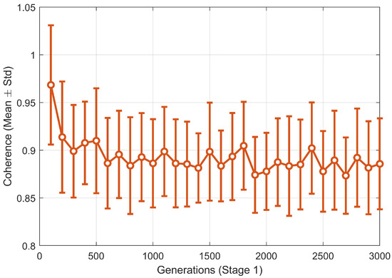
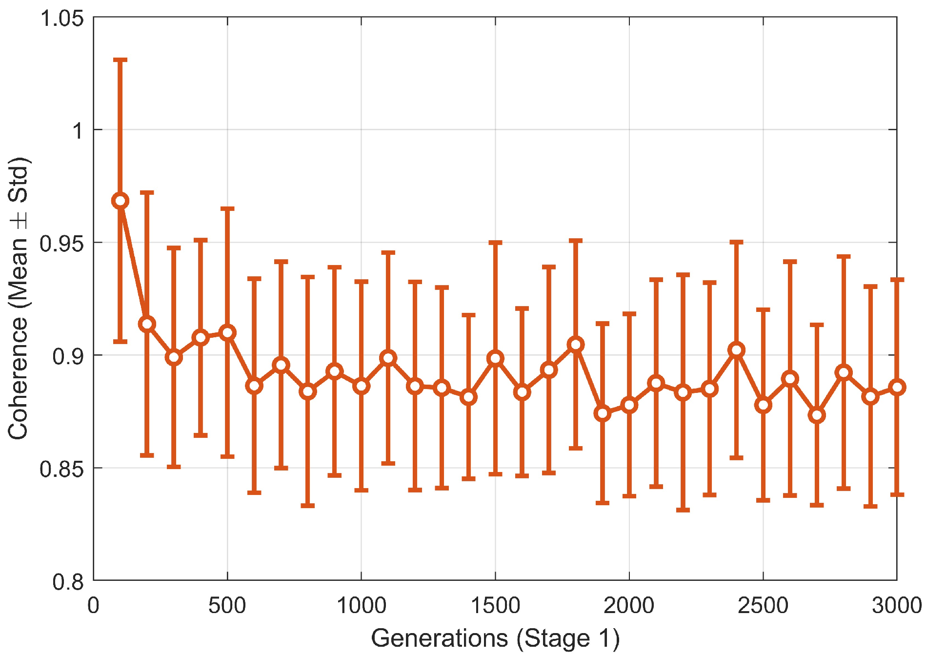
To further analyze the convergence characteristics and verify performance using a reduced number of iterations, we conducted additional Monte Carlo statistical experiments. The convergence curves are shown in Figure 12.

Figure 12. Convergence curve across iterations.

During the first 400 iterations, the coherence metric of the sensing matrix decreases rapidly, attributed to the global exploration capability of the PSO within the first stage hybrid algorithm. By approximately 600 iterations, both the mean and standard deviation of the objective function enter a stable region. Increasing the iterations further to 1500 or even 3000 yields only marginal improvements, with the variance remaining essentially constant.

The choice of 1500 iterations in the original manuscript was primarily based on robustness considerations: the first stage involves a dynamic transition from PSO to CMA-ES. Setting the limit at 1500 ensures that CMA-ES has a sufficient number of generations for refined local search after the switch occurs. The Monte Carlo results demonstrate that in practical engineering applications, limiting the iterations to 600–800 provides an ideal balance between computational time and configuration performance, further highlighting the efficiency of the proposed decoupling strategy.

6.3. Influence of the Number of UAVs

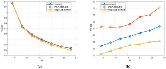
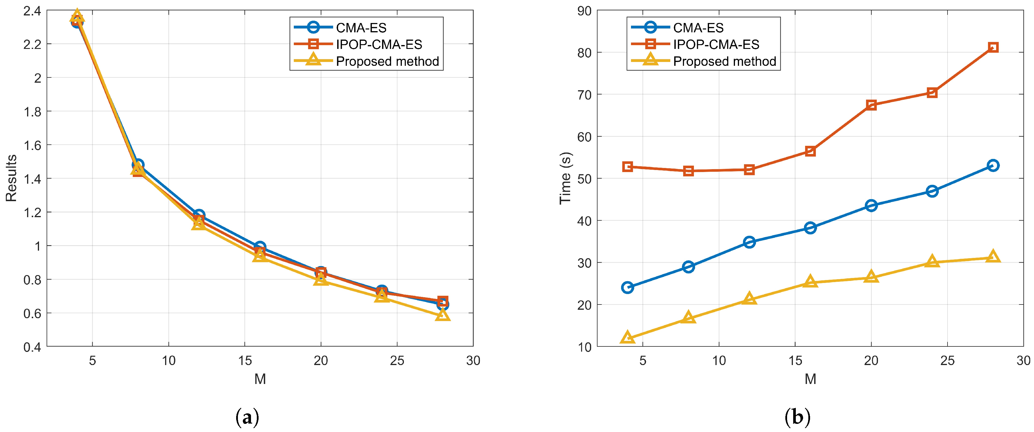
In order to better analyze the applicable scenarios of this method, we evaluated the optimization results and optimization efficiency for swarms ranging from 4 to 28 UAVs. The results of these experiments are summarized in Figure 13.

Figure 13. Influence of the number of UAVs on algorithm performance. (a) Optimization results; (b) optimization time.

The optimization results (governed by the sensing matrix performance) consistently improve as the number of UAVs increases. This is a direct consequence of the increased number of sampling points in the elevation aperture. Conversely, the optimization time increases with the swarm size due to the expansion of the decision variable space.

For $M=4$, the reconstruction performance is inherently limited by insufficient sampling, rendering configuration optimization less meaningful. At $M=8$, IPOP-CMA-ES yields slightly better results. This is because within the specified observation volume, the spatial constraints are relatively sparse for only eight UAVs. In this loose search space, direct 3D optimization can effectively balance the dual objectives of imaging performance and compactness, whereas our proposed method prioritizes the baseline domain in its first stage, which may slightly constrain the compactness search.

As the number of UAVs increases from 12 to 28, the proposed method consistently outperforms the direct 3D optimization algorithms. This advantage stems from the fact that a larger swarm significantly fragments the feasible region in 3D space due to safety separation and mainlobe avoidance constraints. Direct 3D search methods (CMA-ES and IPOP-CMA-ES) frequently become trapped in local optima within these fragmented corridors, whereas our decoupled recursive strategy maintains robust global performance by simplifying the search dimensionality.

In terms of computational efficiency, The proposed method demonstrates a significant advantage in processing speed across all swarm sizes. This efficiency is a direct result of the “space dimensionality reduction” strategy, which reduces the complexity of the global search from 3D coordinates to 1D baseline vectors.

In summary, the proposed optimization is most applicable and advantageous for application scenarios requiring compact distribution, where it offers superior reconstruction quality and significantly lower computational overhead compared to traditional meta-heuristic methods.

6.4. Influence of Position Perturbation on Optimized Configuration

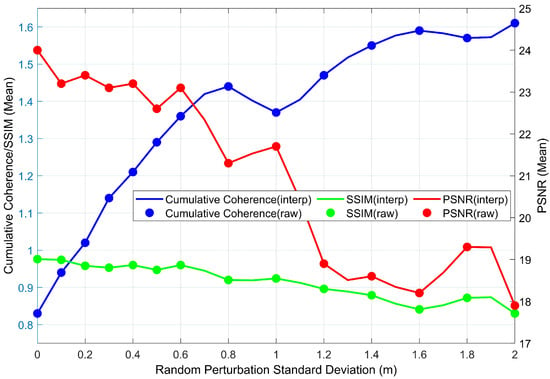
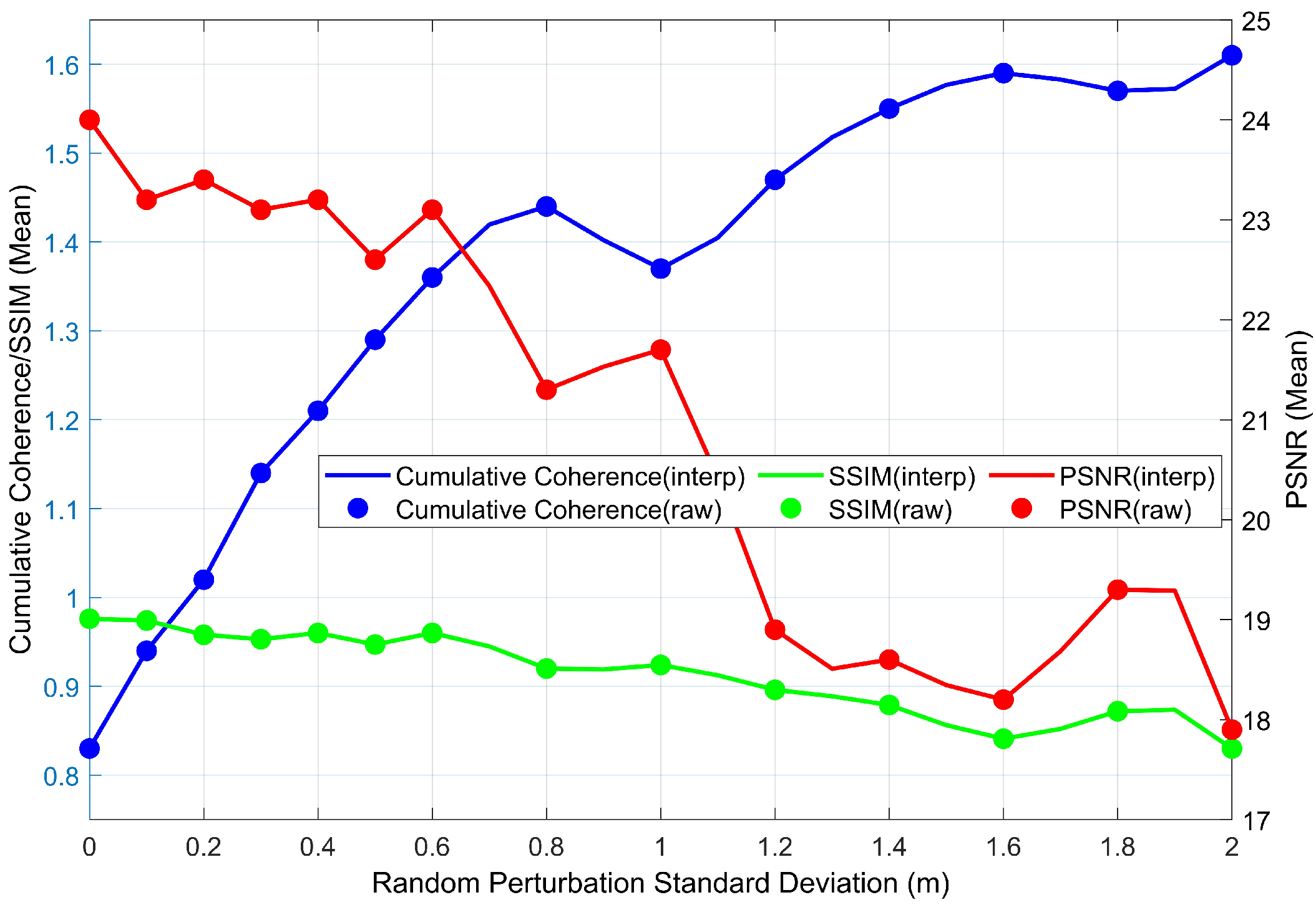
In real-world flight missions, environmental factors such as turbulence, positioning errors, and variable wind fields present non-negligible challenges to the stability of the optimized configuration. To evaluate the robustness of the optimized configuration under non-ideal conditions, we conducted a sensitivity analysis. Random Gaussian perturbations were introduced with standard deviations ranging from 0 to 2 m to the coordinates. For each noise level, 32 independent Monte Carlo trials were performed on the “Z” target profile. The results are illustrated in Figure 14.

Figure 14. Variation of cumulative coherence, SSIM, and PSNR with increasing position perturbation.

It can be observed from the simulation results that the reconstruction performance generally follows a degrading trend as the standard deviation of the random perturbation increases. Within the perturbation range of 0 to 1 m, the system undergoes a rapid decline phase where performance is highly sensitive to displacement, after which it gradually converges to the baseline level of a non-optimized random configuration.

Notably, the slight performance uptick observed at the perturbation point reflects the non-monotonic characteristics of the sensing matrix properties within a highly fragmented feasible region. This suggests that specific random displacements may occasionally yield a baseline arrangement that is statistically more favorable for suppressing sidelobes—a phenomenon we term “accidental optimization.” Despite this localized fluctuation, the quantitative analysis confirms that the optimized configuration maintains a significant performance margin over the random baseline as long as the baseline perturbation is kept within 0.8 m. Once the perturbation exceeds the threshold, the coherence degradation caused by positioning errors largely neutralizes the advantages provided by the pre-mission optimization.

In addition, positioning and time synchronization errors are inevitable in practical distributed SAR systems. Positioning errors primarily cause baseline jitter, while time synchronization errors introduce inter-channel phase offsets. Both factors lead to a mismatch between the measured echo data and the sensing matrix, ultimately manifesting as elevation axis shifts and inversion artifacts in the 3D reconstruction. While this study focuses on optimal pre-mission configuration planning, the development of robust error compensation and joint calibration algorithms will be a prioritized direction for future research.

7. Conclusions

This paper addresses configuration optimization in a distributed UAV SAR system for 3D imaging, subject to stringent imaging quality demands and complex spatial constraints. First, within the framework of compressed sensing theory, sensing matrix cross-correlation is established as a decisive factor governing sparse 3D imaging performance. A multi-objective optimization model is subsequently formulated to minimize the K-order cumulative coherence while enhancing system compactness. Furthermore, practical operational constraints are analyzed, leading to a composite constraint model that incorporates 3D span limits, a flight safety ellipsoid, and mainlobe avoidance based on a double-cone beam model.

To solve the resulting high-dimensional optimization problem with a fragmented feasible region, we propose an efficient algorithm based on a decoupled recursive optimization strategy. The strategy decomposes the original spatial optimization task into two subproblems: global baseline planning and 3D coordinate mapping. In the first stage, a hybrid PSO-CMA-ES algorithm rapidly searches for a globally optimal baseline distribution. In the second stage, analytical geometric pruning and a backtracking mechanism generate a 3D configuration while strictly satisfying physical constraints. Finally, simulation experiments validate the proposed method.

Our results show that compared with an undesigned random distribution, the proposed optimized configuration significantly reduces sensing matrix cross-correlation. Imaging tests on both a profile target and a complex building target produce clearer structural details and fewer erroneous outliers under the optimized configuration. The reconstructed point clouds are closer to the reference point cloud, and improvements are achieved in PSNR, SSIM, as well as point cloud reconstruction accuracy and completeness. Therefore, the proposed method offers a robust and efficient solution for the pre-mission planning of distributed UAV SAR systems, paving the way for their practical application in rapid, high-resolution 3D mapping.

References

- Reigber, A.; Moreira, A.; Papathanassiou, K.P. First demonstration of airborne SAR tomography using multibaseline L-band data. In Proceedings of the IEEE 1999 International Geoscience and Remote Sensing Symposium (IGARSS’99), Hamburg, Germany, 28 June–2 July 1999; Volume 1, pp. 44–46. [Google Scholar]
- Yang, Y.; Zhang, F.; Tian, Y.; Chen, L.; Wang, R.; Wu, Y. High-Resolution and Wide-Swath 3D Imaging for Urban Areas Based on Distributed Spaceborne SAR. Remote Sens. 2023, 15, 3938. [Google Scholar] [CrossRef] [Scilit]
- Zhu, X.X.; Bamler, R. Superresolving SAR tomography for multidimensional imaging of urban areas: Compressive sensing-based TomoSAR inversion. IEEE Signal Process. Mag. 2014, 31, 51–58. [Google Scholar] [CrossRef] [Scilit]
- Peng, X.; Li, X.; Du, Y.; Xie, Q. Forest Height Estimation from a Robust TomoSAR Method in the Case of Small Tomographic Aperture with Airborne Dataset at L-Band. Remote Sens. 2021, 13, 2147. [Google Scholar] [CrossRef] [Scilit]
- Wan, X.; Li, Z.; Chen, E.; Zhao, L.; Zhang, W.; Xu, K. Forest Aboveground Biomass Estimation Using Multi-Features Extracted by Fitting Vertical Backscattered Power Profile of Tomographic SAR. Remote Sens. 2021, 13, 186. [Google Scholar] [CrossRef] [Scilit]
- Liu, X.; Zhang, L.; Yang, X.; Liao, M.; Li, W. Retrieval of Tropical Forest Height and Above-Ground Biomass Using Airborne P- and L-Band SAR Tomography. IEEE Geosci. Remote Sens. Lett. 2022, 19, 4012405. [Google Scholar] [CrossRef] [Scilit]
- Zeng, T.; Liu, M.; Wang, Y.; Ding, Z.; Li, L.; Wang, Z.; Wei, Y.; Wang, J. Tomographic SAR imaging with large elevation aperture: A P-band small UAV demonstration. Sci. China Inf. Sci. 2022, 65, 132303. [Google Scholar] [CrossRef] [Scilit]
- Sun, Y.; Li, L.; Ding, Z.; Wang, Y.; Ma, X.; Sun, X. Preliminary results of UAV ultrawideband SAR tomography based on multi-pass data. In Proceedings of the International Conference on Radar Systems (RADAR 2022), Hybrid Conference, Edinburgh, UK, 24–27 October 2022; pp. 43–47. [Google Scholar]
- Wang, Z.; Ding, Z.; Sun, T.; Zhao, J.; Wang, Y.; Zeng, T. UAV-Based P-Band SAR Tomography With Long Baseline: A Multimaster Approach. IEEE Trans. Geosci. Remote Sens. 2023, 61, 5207221. [Google Scholar] [CrossRef] [Scilit]
- Gao, S.; Wang, W.; Wang, M.; Zhang, Z.; Yang, Z.; Qiu, X.; Zhang, B.; Wu, Y. A Robust Super-Resolution Gridless Imaging Framework for UAV-Borne SAR Tomography. IEEE Trans. Geosci. Remote Sens. 2024, 62, 5210917. [Google Scholar] [CrossRef] [Scilit]
- Hu, F.; Wang, F.; Ren, Y.; Xu, F.; Qiu, X.; Ding, C.; Jin, Y. Error analysis and 3D reconstruction using airborne array InSAR images. ISPRS J. Photogramm. Remote Sens. 2022, 190, 113–128. [Google Scholar] [CrossRef] [Scilit]
- Li, X.; Zhang, F.; Liang, X.; Li, Y.; Guo, Q.; Wan, Y.; Bu, X.; Liu, Y. Fourfold Bounce Scattering-Based Reconstruction of Building Backs Using Airborne Array TomoSAR Point Clouds. Remote Sens. 2022, 14, 1937. [Google Scholar] [CrossRef] [Scilit]
- Ren, H.; Sun, Z.; Yang, J.; Xiao, Y.; An, H.; Li, Z.; Wu, J. Swarm UAV SAR for 3-D Imaging: System Analysis and Sensing Matrix Design. IEEE Trans. Geosci. Remote Sens. 2022, 60, 5238316. [Google Scholar] [CrossRef] [Scilit]
- Khan, A.; Jhanjhi, N.Z. Growth of Drones: Opportunities and Risks. In Cybersecurity Issues and Challenges in the Drone Industry; Shah, I.A., Jhanjhi, N.Z., Eds.; IGI Global Scientific Publishing: Hershey, PA, USA, 2024; pp. 452–486. [Google Scholar]
- Harmer, S.W.; De Novi, G. Distributed Antenna in Drone Swarms: A Feasibility Study. Drones 2023, 7, 126. [Google Scholar] [CrossRef] [Scilit]
- Li, W.; Ma, Y.; Ma, X.; Li, B.; Zhao, X.; Xi, L. A 3D Imaging Method for UAV Swarm Polarimetric SAR Based on Joint Sparse and Low-Rank Structure Constraints. IET Image Process. 2025, 19, e70200. [Google Scholar] [CrossRef] [Scilit]
- Zhou, H.; Xu, G.; Xia, X.-G.; Li, T.; Yu, H.; Liu, Y.; Zhang, X.; Xing, M.; Hong, W. Enhanced Matrix Completion Method for Superresolution Tomography SAR Imaging: First Large-Scale Urban 3-D High-Resolution Results of LT-1 Satellites Using Monostatic Data. IEEE J. Sel. Top. Appl. Earth Observ. Remote Sens. 2025, 18, 22743–22758. [Google Scholar] [CrossRef] [Scilit]
- Liu, C.; Wang, Y.; Zhang, G.; Ding, Z. High Resolution Large Elevation Synthetic Aperture Tomographic SAR Imaging With Classifier-Based Imaging Architecture. IEEE J. Sel. Top. Appl. Earth Observ. Remote Sens. 2025, 18, 20666–20677. [Google Scholar] [CrossRef] [Scilit]
- Wang, L.; Xiang, W.; Song, H.; Zhang, H.; Zheng, M.; Wang, J.; Xue, F.; Ai, Z.; Deng, Y. A Novel Phase Calibration Method for Airborne P-, L-, and S-Band SAR Tomography Based on Weighted Phase Gradient Autofocus. IEEE Trans. Geosci. Remote Sens. 2025, 63, 1–20. [Google Scholar] [CrossRef] [Scilit]
- Zhu, X.X.; Bamler, R. Tomographic SAR Inversion by l1-Norm Regularization—The Compressive Sensing Approach. IEEE Trans. Geosci. Remote Sens. 2010, 48, 3839–3846. [Google Scholar] [CrossRef] [Scilit]
- Candès, E.J.; Romberg, J.; Tao, T. Robust uncertainty principles: Exact signal reconstruction from highly incomplete frequency information. IEEE Trans. Inf. Theory 2006, 52, 489–509. [Google Scholar] [CrossRef] [Scilit]
- Donoho, D.L. Compressed sensing. IEEE Trans. Inf. Theory 2006, 52, 1289–1306. [Google Scholar] [CrossRef] [Scilit]
- Ben-Haim, Z.; Eldar, Y.C.; Elad, M. Coherence-Based Performance Guarantees for Estimating a Sparse Vector Under Random Noise. IEEE Trans. Signal Process. 2010, 58, 5030–5043. [Google Scholar] [CrossRef] [Scilit]
- Obermeier, R.; Martinez-Lorenzo, J.A. Sensing Matrix Design via Mutual Coherence Minimization for Electromagnetic Compressive Imaging Applications. IEEE Trans. Comput. Imaging 2017, 3, 217–229. [Google Scholar] [CrossRef] [Scilit]
- An, H.; Shen, M.; Wang, C.; Ren, H.; Mao, X.; Wu, J.; Li, Z.; Yang, J. Multistatic Synthetic Aperture Radar Baseline Design for 3-D Imaging. In Proceedings of the IGARSS 2022—2022 IEEE International Geoscience and Remote Sensing Symposium, Kuala Lumpur, Malaysia, 17–22 July 2022; pp. 2502–2505. [Google Scholar]
- Seker, I.; Lavalle, M. Tomographic Performance of Multi-Static Radar Formations: Theory and Simulations. Remote Sens. 2021, 13, 737. [Google Scholar] [CrossRef] [Scilit]
- Chen, Z.; Hu, C.; Dong, X.; Li, Y.; Tian, W.; Hobbs, S. Coherence-Based Geosynchronous SAR Tomography Employing Formation Flying: System Design and Performance Analysis. IEEE Trans. Geosci. Remote Sens. 2021, 59, 7165–7179. [Google Scholar] [CrossRef] [Scilit]
- Bi, H.; Liu, J.; Zhang, B.; Hong, W. Baseline distribution optimization and missing data completion in wavelet-based CS-TomoSAR. Sci. China Inf. Sci. 2018, 61, 042302. [Google Scholar] [CrossRef] [Scilit]
- Zhao, J.; Yu, A.; Zhang, Y.; Zhu, X.; Dong, Z. Spatial Baseline Optimization for Spaceborne Multistatic SAR Tomography Systems. Sensors 2019, 19, 2106. [Google Scholar] [CrossRef] [Scilit] [PubMed]
- Wei, L.; Feng, Q.; Liu, S.; Bignami, C.; Tolomei, C.; Zhao, D. Minimum Redundancy Array—A Baseline Optimization Strategy for Urban SAR Tomography. Remote Sens. 2020, 12, 3100. [Google Scholar] [CrossRef] [Scilit]
- Fasano, G.; Renga, A.; D’Errico, M. Formation geometries for multistatic SAR tomography. Acta Astronaut. 2014, 96, 11–22. [Google Scholar] [CrossRef] [Scilit]
- Ao, Y.; Feng, D.; An, D. A baseline distribution scheme for swarm UAVs multi-static SAR tomographic imaging. In Proceedings of the IET International Radar Conference (IRC 2023), Chongqing, China, 3–5 December 2023; pp. 3252–3258. [Google Scholar]
- Wang, C.; Li, Z.; Hai, Y.; An, H.; Wu, J.; Yang, J. Multistatic TomoSAR 3-D Imaging Technique via Matrix Completion for Structured Targets. IEEE Trans. Geosci. Remote Sens. 2025, 63, 5215716. [Google Scholar] [CrossRef] [Scilit]
- Tropp, J.A. Greed is good: Algorithmic results for sparse approximation. IEEE Trans. Inf. Theory 2004, 50, 2231–2242. [Google Scholar] [CrossRef] [Scilit]
- Guo, L.; Yue, J. Analysis of Coherence Effected by Baseline and Time Interval. Bull. Surv. Mapp. 2018, 7, 9–12. (In Chinese) [Google Scholar]
- Gatelli, F.; Monti Guarnieri, A.; Parizzi, F.; Pasquali, P.; Prati, C.; Rocca, F. The wavenumber shift in SAR interferometry. IEEE Trans. Geosci. Remote Sens. 1994, 32, 855–865. [Google Scholar] [CrossRef] [Scilit]
- Clerc, M.; Kennedy, J. The particle swarm—Explosion, stability, and convergence in a multidimensional complex space. IEEE Trans. Evol. Comput. 2002, 6, 58–73. [Google Scholar] [CrossRef] [Scilit]
- Hansen, N. The CMA Evolution Strategy: A Tutorial. arXiv 2016, arXiv:1604.00772. [Google Scholar] [CrossRef] [Scilit]
- Auger, A.; Hansen, N. A restart CMA evolution strategy with increasing population size. In Proceedings of the 2005 IEEE Congress on Evolutionary Computation (CEC 2005), Edinburgh, UK, 2–5 September 2005; Volume 2, pp. 1769–1776. [Google Scholar]
- Bioucas-Dias, J.M.; Figueiredo, M.A.T. A New TwIST: Two-Step Iterative Shrinkage/Thresholding Algorithms for Image Restoration. IEEE Trans. Image Process. 2007, 16, 2992–3004. [Google Scholar] [CrossRef] [Scilit]
- Wipf, D.P.; Rao, B.D. An Empirical Bayesian Strategy for Solving the Simultaneous Sparse Approximation Problem. IEEE Trans. Signal Process. 2007, 55, 3704–3716. [Google Scholar] [CrossRef] [Scilit]
- Das, S.; Suganthan, P.N. Differential Evolution: A Survey of the State-of-the-Art. IEEE Trans. Evol. Comput. 2011, 15, 4–31. [Google Scholar] [CrossRef] [Scilit]
- Poli, R.; Kennedy, J.; Blackwell, T. Particle swarm optimization. Swarm Intell. 2007, 1, 33–57. [Google Scholar] [CrossRef] [Scilit]
- Kirkpatrick, S.; Gelatt, C.D.; Vecchi, M.P. Optimization by Simulated Annealing. Science 1983, 220, 671–680. [Google Scholar] [CrossRef] [Scilit]
Disclaimer/Publisher’s Note: The statements, opinions and data contained in all publications are solely those of the individual author(s) and contributor(s) and not of MDPI and/or the editor(s). MDPI and/or the editor(s) disclaim responsibility for any injury to people or property resulting from any ideas, methods, instructions or products referred to in the content. |
© 2026 by the authors. Licensee MDPI, Basel, Switzerland. This article is an open access article distributed under the terms and conditions of the Creative Commons Attribution (CC BY) license.