Contrastive Masked Feature Modeling for Self-Supervised Representation Learning of High-Resolution Remote Sensing Images

Highlights

What are the main findings?

• A self-supervised learning framework was developed for remote sensing semantic segmentation.
• Combining contrastive learning and masked image modeling during pretraining improved feature representation.

What are the implications of the main findings?

• Our method enables accurate segmentation with limited labels in complex scenes.
• Hybrid CNN+Transformer SSL shows strong potential for high-resolution remote sensing segmentation.

Abstract

As an emerging learning paradigm, self-supervised learning (SSL) has attracted extensive attention due to its ability to mine features with effective representation from massive unlabeled data. In particular, SSL, driven by contrastive learning and masked modeling, shows great potential in general visual tasks. However, because of the diversity of ground target types, the complexity of spectral radiation characteristics, and changes in environmental conditions, existing SSL frameworks exhibit limited feature extraction accuracy and generalization ability when applied to complex remote sensing scenarios. To address this issue, we propose a hybrid SSL framework that integrates the advantages of contrastive learning and masked modeling to extract more robust and reliable features from remote sensing images. The proposed framework includes two parallel branches: one branch uses a contrastive learning strategy to strengthen global feature representation and capture image structural information by constructing positive and negative sample pairs; the other branch adopts a masked modeling strategy, focusing on the fine analysis of local details and predicting the features of masked areas, thereby establishing connections between global and local features. Additionally, to better integrate local and global features, we adopt a hybrid CNN+Transformer architecture, which is particularly suitable for intensive downstream tasks such as semantic segmentation. Extensive experimental results demonstrate that the proposed framework not only exhibits superior feature extraction ability and higher accuracy in small-sample scenarios but also outperforms state-of-the-art mainstream SSL frameworks on large-scale datasets.

1. Introduction

With the continuous advancement of remote sensing technology, high-resolution satellite and aerial imagery have become indispensable tools for Earth observation. These technologies are now widely applied in various domains, including natural resource management, urban planning, and disaster response. In recent years, deep learning-based artificial intelligence algorithms have achieved significant breakthroughs in large-scale remote sensing image analysis [1]. This progress has not only spurred technological innovation but also emerged as a focal point of current research, charting a new course for the long-term development of remote sensing image analysis.

Despite these advancements, several challenges persist in remote sensing image analysis that require addressing. Firstly, the complexity and cost of data annotation present significant hurdles. The intricate diversity of remote sensing data and the substantial costs associated with obtaining high-quality annotations necessitate considerable time and financial investment, particularly for tasks requiring specialized knowledge. This challenge severely limits the scale and quality improvements of datasets. Secondly, traditional deep learning methods encounter difficulties in small-sample learning scenarios. While deep convolutional neural networks (e.g., ResNet [2]) and Vision Transformers (e.g., ViT [3]) excel in feature representation, they tend to inadequately learn effective representations when faced with extremely limited samples from specific categories. Such scarcity can lead to overfitting, thereby impacting the model’s prediction performance on new, unseen data. Lastly, the inherent variability of remote sensing imagery introduces another layer of complexity. Variations in shooting angles, distances, and lighting conditions between images of the same category [4] introduce substantial differences, making it challenging to accurately identify and extract discriminative key features from these complex and variable images. Addressing these challenges requires approaches capable of effectively leveraging vast amounts of unlabeled data while minimizing dependency on extensive labeled datasets. Moreover, developing models that can robustly generalize from limited training samples and adapt to diverse imaging conditions is crucial for advancing the field of remote sensing image analysis.

To address these challenges, particularly the issues of annotation scarcity and small-sample learning, self-supervised learning (SSL) has emerged as a critical approach for remote sensing image analysis due to its distinctive advantages. By uncovering the intrinsic structure and features of data, SSL enables models to learn deeper potential representations without relying on large annotated datasets. This significantly enhances the abstraction and high-dimensional feature expression capabilities of remote sensing images while greatly reducing the manual workload required for creating annotated labels during model training. In recent years, SSL has achieved remarkable success in the field of computer vision and has gradually permeated into remote sensing image analysis, providing a new avenue to tackle these challenges.

Among the various SSL paradigms, masked modeling and contrastive learning are two common and effective strategies in the field of SSL for image processing. Contrastive learning, as a widely regarded SSL strategy, trains models by learning the similarities and differences between different data representations. However, contrastive learning focuses on global feature representation and tends to underperform in tasks requiring precise location information. Recent studies have revealed specific failure scenarios for contrastive learning methods in remote sensing applications. For instance, when applied to high-resolution urban remote sensing images containing dense building clusters, contrastive learning methods struggle to distinguish between structurally similar buildings, often exhibiting reduced IoU performance on building extraction tasks compared to supervised methods. This performance degradation stems from the method’s reliance on global image-level representations, which fail to capture fine-grained spatial details essential for precise boundary delineation in dense urban environments. Additionally, contrastive learning exhibits performance drops when processing multi-temporal remote sensing sequences, where seasonal variations in vegetation and illumination conditions create inconsistent feature representations, leading to temporal misalignment issues that reduce semantic segmentation accuracy compared to single-temporal analysis.

Masked modeling, another efficient SSL strategy, involves learning image feature representations by predicting masked regions. However, it exhibits distinct failure patterns when dealing with remote sensing imagery. Specifically, masked autoencoders show performance degradation in scenarios involving spectrally similar land cover types. When applied to agricultural remote sensing images for crop classification, reconstruction-based methods demonstrate reduced accuracy for distinguishing between spectrally similar crops compared to supervised approaches [5]. This limitation occurs because the reconstruction objective focuses on pixel-level recovery rather than semantic understanding, leading to confusion between classes with similar spectral signatures but different agricultural significance. Furthermore, masked modeling approaches may face challenges in small-object detection scenarios common in remote sensing, such as vehicle or building detection in high-resolution imagery. The random masking strategy can obscure small targets, potentially preventing the model from learning their characteristic features [6]. Additionally, masked modeling methods may exhibit systematic biases toward texture-rich regions while neglecting smooth areas like water bodies or homogeneous agricultural fields, leading to unbalanced feature representations that compromise downstream task performance [7].

These empirical observations highlight a fundamental limitation: single-strategy SSL approaches fail to address the multifaceted complexity of remote sensing imagery analysis. Contrastive learning’s global focus sacrifices local precision, while masked modeling’s local reconstruction neglects global context and semantic relationships. This trade-off becomes particularly problematic in remote sensing applications where both global scene understanding and local detail preservation are crucial for tasks such as semantic segmentation, change detection, and land cover classification.

Given these complementary strengths and weaknesses, a natural question arises: can we combine contrastive learning and masked modeling to leverage their respective advantages while mitigating their individual limitations? Theoretically, contrastive learning enhances global feature representation, while masked modeling pays more attention to capturing local details. Recent theoretical analysis by Chen et al. [8] demonstrated that combining these complementary strategies can theoretically achieve better representation learning bounds, suggesting that hybrid approaches may overcome the individual limitations of each method. Building on this insight, Zhang et al. [9] proposed a multi-modal fusion framework that integrates contrastive and reconstructive objectives for medical image analysis, achieving state-of-the-art performance on multiple benchmarks.

To this end, we propose an innovative dual-branch SSL framework in this paper to improve image feature representation in remote sensing scenarios. The framework adopts a hybrid CNN+Transformer network, comprising two branches: one for contrastive learning and the other for masked modeling, allowing the model to leverage the strengths of both strategies. In the masked modeling branch, we implement masked feature modeling (MFM) [10] adapted to the CNN+Transformer hybrid architecture. Additionally, we design a composite loss function to balance the objectives of the two branches—contrastive learning and masked modeling—thereby guiding the overall learning process more effectively. This loss function consists of two components: a contrastive loss and a reconstruction loss. By optimizing these two losses, the model learns a more complete and context-sensitive feature representation while maintaining feature discrimination.

To verify the effectiveness of the proposed framework, we conducted extensive experiments using three public remote sensing image datasets and compared them with state-of-the-art SSL methods. Experimental results show that our method performs well across multiple downstream tasks, further confirming the effectiveness of integrating contrastive learning and MFM strategies to enhance the feature learning effect of remote sensing images.

The main contributions of this paper are as follows:

• We propose a self-supervised learning (SSL) framework tailored for semantic segmentation tasks of high-resolution remote sensing images. This framework fully leverages the advantages of both contrastive learning and masked feature modeling strategies, enabling the model to simultaneously learn robust global features and fine-grained local features in high-resolution remote sensing images, thereby effectively enhancing the quality of feature representation.
• The framework adopts a hybrid CNN+Transformer architecture that fully exploits the local modeling advantages of CNNs and the global context modeling capabilities of Transformers, effectively compensating for the local detail loss caused by pure Transformer architectures.
• Extensive experiments on three publicly available high-resolution remote sensing image datasets show that our method achieves superior performance over existing state-of-the-art self-supervised learning approaches. Furthermore, ablation studies demonstrate the contribution of each module to the overall performance.

The rest of this study is organized as follows. Section 2 describes related works on SSL. Section 3 provides details of the proposed method. Experimental results and analyses are presented in Section 4. Conclusions are drawn in Section 5.

2. Related Works

In recent years, SSL, a paradigm that does not require the manual labeling of data, has achieved remarkable results in the field of computer vision. The core idea is to automatically mine supervisory signals from unlabeled data for model training, thereby effectively alleviating the dependence of supervised learning on large amounts of labeled data. In high-cost, time-consuming annotation scenarios, such as remote sensing image analysis, SSL has become an important means to enhance the generalization ability of models.

2.1. Contrastive Learning

As one of the key methods in SSL, contrastive learning trains models to distinguish between similar and non-similar samples by constructing pairs of positive and negative samples. This strategy aims to minimize the distance between similar samples in the embedding space while maximizing the distance between dissimilar ones, thereby facilitating the model’s understanding of the data’s internal structure. In recent years, contrastive learning has achieved significant advances in computer vision, as exemplified by frameworks like SimCLR [11] and Momentum Contrast (MoCo) [12], which have demonstrated its effectiveness in image classification tasks. SimCLR employs data augmentation techniques to generate diverse views of the same image as positive sample pairs for training; MoCo introduces a momentum encoder along with a dynamic update queue mechanism to achieve an efficient and stable contrastive learning process. Bootstrap Your Own Latent (BYOL) [13] proposes a novel two-tower architecture—an online network and a target network—wherein the online network’s weights are updated via exponential moving averages, enabling the learning of high-quality feature representations without the need for explicit negative examples. The SwAV method [14] enhances both the robustness and generalization ability of models under conditions of small batch sizes by introducing cluster-based objectives and encouraging the assignment of different augmented views of the same instance to the same cluster. Self-supervised Contrastive Segmentation (SeCo) [15] further broadens the application scope of contrastive learning by capturing local and global information through pixel-level and feature-level contrastive learning, significantly improving feature representation in semantic segmentation tasks.

2.2. Masked Modeling

The concept of masked modeling originated in the field of natural language processing (NLP), with the most representative application being the Bidirectional Encoder Representations from Transformers (BERT) model [16]. BERT trains a bidirectional Transformer architecture using a masked language model (MLM), enabling it to learn high-quality language representations under unsupervised conditions. In this process, some words within the input text sequence are randomly masked, and the model’s task is to predict these masked tokens. This technology has driven advancements in NLP and inspired a series of mask-based autoencoding models, such as RoBERTa [17] and ALBERT [18].

Inspired by the success of masked modeling in NLP, this concept has gradually been introduced into computer vision. Masked Image Modeling (MIM) adopts the core idea of MLM to train models to predict the content of occluded parts by randomly masking specific areas of an input image. A Masked Autoencoder (MAE) [19] is a classic example of MIM, where a masked autoencoder recovers the missing parts of an image, thereby learning rich image feature representations. Subsequent advancements, such as a Masked Autoencoder for 3D Mesh Data Analysis (MeshMAE) [20] and Masked Autoencoder for Video (VideoMAE) [21], have demonstrated excellent performance across various vision tasks. SimMIM [22] employs a similar masking strategy but innovatively replaces the masked blocks with learnable vectors and uses simple linear layers for reconstruction, achieving good results. A Context Autoencoder (CAE) [23] is a masked image modeling method that strictly separates the representation learning role from the pretext task completion role, ensuring that the encoder focuses on image feature learning during SSL training and enhancing the model’s generalization to downstream tasks.

2.3. Self-Supervised Learning of Remote Sensing Images

Inspired by the latest advances in computer vision, the field of remote sensing has begun to actively explore SSL models suitable for various scenarios. Regarding SSL of remote sensing images based on contrastive learning, Kang et al. [24] proposed the Spatially Augmented Momentum Contrast Model (SauMoCo), building upon the MoCo framework. SauMoCo enhances the description of label-free remote sensing scenes through spatial augmentation technology. Jung et al. [25] developed a remote sensing contrastive SSL method with smooth representation characteristics based on the SimCLR framework. This method effectively captures the diversity and complexity of remote sensing images by averaging the representations of multiple input images. Li et al. [26] introduced a Global–Local Contrastive Network (GLCNet), which features a global contrastive learning module to capture image-level representations and integrates it with a local feature matching contrastive learning module to refine the representations of local regions, thereby significantly improving the accuracy of semantic segmentation. Guan and Lam [27] designed a cross-domain contrastive learning framework that enables the model to learn discriminative feature representations unaffected by domain differences. This is achieved by comparing sample pairs from the same and different domains.

However, traditional contrastive learning methods have limitations when processing semantic segmentation tasks involving high-resolution remote sensing images. These methods struggle to provide sufficient spatial detail [28] and often require a large number of negative samples to ensure accurate discrimination between positive and negative samples. This increases computational burden and limits application in resource-constrained environments [29].

In terms of SSL of remote sensing images based on masked modeling, Cong and Khanna [30] proposed SatMAE, a pre-trained framework for temporal or multispectral satellite images. Based on the MAE algorithm, SatMAE effectively encodes spatiotemporal features of multispectral data through temporal embedding and cross-time independent masking strategies. Pang et al. [10] proposed MFM, which combines the advantages of CNN and Transformer architectures to achieve SSL by masking some features from the output of CNN modules. Tang et al. [31] proposed a SSL architecture for multimodal remote sensing images, capable of extracting high-level feature representations from multi-view data and combining them with spectral information for land cover classification. Beyond single-modality approaches, recent advances have explored multi-modal SSL methods and foundation model-based pre-training paradigms. Wang et al. [32] developed spectral-spatial-temporal Transformers that integrate temporal sequences of hyperspectral imagery for change detection, demonstrating enhanced capability in capturing multi-temporal dynamics. Muhuri et al. [33] systematically reviewed the integration of SAR and optical data for SSL, emphasizing that fusion of active and passive sensor modalities enables robust feature learning under diverse atmospheric conditions. Furthermore, Wang et al. [34] introduced SAMRS, leveraging the Segment Anything Model to create a large-scale segmentation dataset that enables pre-training of foundation models with zero-shot and few-shot generalization capabilities, representing a paradigm shift toward general-purpose visual representation learning in Earth observation applications.

In conclusion, in the field of remote sensing image processing, most existing methods rely on a single SSL strategy: some focus on learning global distinguishable representations through contrastive learning, while others capture local spatial context information via masked modeling. However, when faced with complex remote sensing image processing tasks, these single-strategy approaches often fail to provide sufficient performance and flexibility, leading to limited model performance.

To address this issue, we propose an SSL framework that integrates contrastive learning and MFM, termed Contrastive Masked Feature Modeling (CMFM). CMFM aims to combine the strengths of both strategies, enabling the model to simultaneously learn feature representations with high global discrimination and maintain local spatial integrity. Through this comprehensive method, CMFM not only enhances the richness and accuracy of feature representation but also significantly improves the model’s generalization ability, thereby better meeting the diverse needs of various downstream remote sensing image tasks.

3. Methodology

This section provides an overview of our proposed framework, followed by detailed descriptions of each module.

3.1. Overview

The architecture of the proposed CMFM framework is presented in Figure 1. This framework comprises two main branches: a Contrastive Learning Representation (CLR) branch based on SimCLR architecture and a Masked Feature Modeling (MFM) branch grounded in masked autoencoder. We choose SimCLR as the foundation for the CLR branch due to its demonstrated effectiveness in various remote sensing applications, particularly excelling in multimodal remote sensing image semantic segmentation over other contrastive learning methods like MoCo.

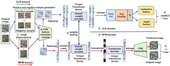
Figure 1. The architecture of the proposed CMFM framework comprising six main components: (1) Image Preprocessing, (2) CNN Feature Extraction, (3) Shared-weight Encoder, (4) CLR Decoder, (5) MFM Decoder, and (6) Loss Function. The framework features dual-branch design with CLR branch (blue pathway) and MFM branch (red pathway) sharing the same encoder.

The entire network encompasses image preprocessing, feature extraction, a shared-weight encoder, CLR decoder, MFM decoder, and a loss function. Image preprocessing prepares inputs suitable for both CLR and MFM tasks by applying data augmentation techniques and constructing positive and negative sample pairs. The feature extraction module employs multi-layer convolution operations to obtain high-order feature maps from images. After feature extraction, features are processed according to specific requirements of each branch: for the CLR branch, the feature map is directly flattened into a 1D sequence; for the MFM branch, a random mask is applied to the feature map, after which unmasked portions are flattened into a 1D sequence. The shared-weight encoder comprises a series of Transformer units that further process 1D sequences to obtain encoding sequences enriched with global context information. The CLR decoder reshapes encoded sequences, applies average pooling, and reduces dimensionality to generate new feature sequences. The MFM decoder utilizes unmasked parts of the encoding sequence for mask concatenation, employs a Transformer decoding block, and applies convolutional upsampling to reconstruct occluded areas. The loss function synthesizes objectives from both CLR and MFM branches, ensuring the model not only differentiates between similar and dissimilar sample pairs but also precisely recovers content of occluded areas when parts of information are missing.

3.2. Image Preprocessing

Image preprocessing processes input raw images to generate two types of data: one specially customized for masked image modeling in the MFM branch, and the other tailored to meet requirements of dual-view contrast learning in the CLR branch. The main purpose is to ensure both branches receive the most suitable data, thereby improving learning efficiency and feature extraction capabilities. The process, shown in Figure 2, includes data augmentation and construction of positive and negative samples.

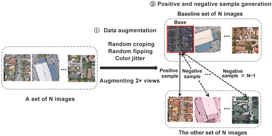
Figure 2. Image preprocessing module.

Data Augmentation:In contrastive learning tasks, the combination of color augmentation and different views can help the model achieve greater invariance among features. For masked image modeling tasks, Gaussian blurring and stochastic grayscale transformations may degrade model performance [6], making it challenging for the model to accurately capture original semantic information. Therefore, we selected three methods: color jittering, random cropping, and random flipping. We optimized the traditional two-branch independent data augmentation strategy by ensuring both branches share the same input. This optimization is achieved by expanding the original image into dual views and simultaneously applying random cropping, flipping, and color jittering. This approach reduces input variance and training noise, enabling the model to learn more consistent, high-quality feature representations.

Construction of Positive and Negative Samples: Given input images in each batch (set to N), we select one of the two new sets of image data generated by data augmentation as the baseline image set. The other set is used to pair with each image in the baseline set to construct pairs of positive and negative samples. Specifically, for each image in the baseline set, its corresponding positive sample is the differently augmented version of the same original image from the other set. Meanwhile, each image in the baseline set forms negative sample pairs with all N−1 non-corresponding images from the other set. This method ensures each image has a unique positive sample and N−1 negative samples, effectively supporting discriminative feature learning in the subsequent contrastive learning process.

3.3. Feature Extraction Module

The feature extraction module extracts multi-scale higher-order features from images. It consists of convolutional feature extraction and feature post-processing, as shown in Figure 3.

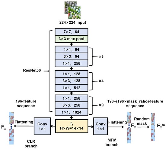
Figure 3. The structure of the feature extraction module.

Convolutional feature extraction: We use the classical ResNet50 network, which extracts high-dimensional, low-resolution deep features from input shallow features. We modified the ResNet50 structure, adjusting the output feature map size from standard $7\times 7$ to $14\times 14$ to retain more local details, especially important for processing remote sensing images containing numerous small targets. The formula is:

$$f_x=\mathrm{ResNet}50\left(x\right)$$

(1)

where x is the augmented image, $f_x\in {\mathbb{R}}^{H/16\times W/16\times C}$ represents the output feature map, H and W are the height and width of the image.

Feature post-processing: After feature extraction, to meet specific requirements of the CLR and MFM branches, output $f_x$ requires further post-processing. For the CLR branch, the 2D feature map of size $14\times 14$ first adjusts channels via a $1\times 1$ convolution, then flattens into a 1D feature sequence $F_x$ of length 196:

$$F_x=\mathrm{flatten}\left({\mathrm{Conv}}_{1\times 1}\left(f_x\right)\right)$$

(2)

where ${\mathrm{Conv}}_{1\times 1}$ represents a convolution operation with kernel size $1\times 1$ and stride 1; flatten converts the 2D $14\times 14$ feature map into a 1D sequence $F_x$ of length 196.

We represent $F_x$ as 196 feature block elements $f_i$ according to their sequence positions:

$$F_x=\{f_1,f_2,f_3,\dots ,f_n\},n={\displaystyle \frac{H}{16}}\times {\displaystyle \frac{W}{16}}$$

(3)

For the MFM branch, a random mask operation is further applied to $F_x$:

$$F_x^{\prime }=F_x\otimes M^T$$

(4)

$$\begin{array}{c}M=\{m_1,m_2,m_3,\dots ,m_n\},\\ m\in \{0,1\},n={\displaystyle \frac{H}{16}}\times {\displaystyle \frac{W}{16}}\end{array}$$

(5)

where M is the mask sequence—a 1D sequence where 0 represents masked feature blocks and 1 represents unmasked feature blocks. The number of 0 s and 1 s in M is determined according to a random mask ratio (ranging from 25% to 80%). $F_x^{\prime }$ denotes element-wise multiplication between $F_x$ and M.

After random masking, we extract the unmasked elements sequence:

$$F_x^m=\left\{f_i^{\prime }|m_i=1,i\in \{1,2,\dots ,n\}\right\}$$

(6)

$$f_i^{\prime }=f_i·m_i$$

(7)

where $f_i^{\prime }$ represents an element in the resulting sequence $F_x^{\prime }$ after multiplying $F_x$ and M element-wise; $F_x^m$ represents the final unmasked sequence containing all elements from $F_x$ at positions where $m=1$.

3.4. Shared-Weight Encoder

The shared-weight encoder processes 1D sequences from both branches, including sequence $F_x$ from the CLR branch and sequence $F_x^m$ from the MFM branch. Through its self-attention mechanism, it effectively captures long-distance dependencies within sequences, enhances feature extraction capabilities, and improves model robustness and generalization. The parameter-sharing scheme reduces parameter redundancy, mitigates overfitting risk, and fosters synergistic effects between both tasks.

The shared-weight encoder adopts a 12-layer stacked Transformer block structure. Each Transformer unit comprises two LayerNorm layers, a multi-head attention mechanism module, and an MLP layer, ensuring consistent input and output feature dimensions across each unit. The shared-weight encoder processes $F_x$ and $F_x^m$ independently but identically. Taking the processing of $F_x$ in the CLR branch as an example, the equations for a single-layer Transformer unit are:

$$F_x^A=F_x+\mathrm{MultiHead}\left(\mathrm{LayerNorm}\left(F_x\right)\right)$$

(8)

$$E_x=F_x^A+\mathrm{MLP}\left(\mathrm{LayerNorm}\left(F_x^A\right)\right)$$

(9)

where MultiHead represents the multi-head attention mechanism, LayerNorm represents the tensor data normalization function, MLP stands for multilayer perceptron, $F_x^A$ represents the output of the first sub-layer (multi-head self-attention with residual connection), and $E_x$ represents the output of the shared-weight encoder after the second sub-layer (feed-forward network with residual connection). This design follows the standard Pre-LN Transformer architecture where LayerNorm is applied before each sub-layer operation (attention or MLP), and the residual connection adds the original input to the sub-layer output. Specifically, LayerNorm normalizes the input before transformation, and the transformed result is then added back to the original input via residual connection. The equation for MultiHead is:

$$\mathrm{MultiHead}\left(F_x\right)=\mathrm{Concat}({\mathrm{head}}_1\left(F_x\right),\dots ,{\mathrm{head}}_h\left(F_x\right))$$

(10)

where Concat represents feature concatenation, ${\mathrm{head}}_i$ is a single attention head. The equation for ${\mathrm{head}}_i$ is:

$$\begin{array}{cc}\hfill {\mathrm{head}}_i\left(F_x\right)& =\mathrm{Attention}(Q_i,K_i,V_i)\hfill \\ \hfill & =\mathrm{Attention}(F_x{W}_i^Q,F_x{W}_i^K,F_x{W}_i^V)\hfill \end{array}$$

(11)

where Attention is the attention calculation function; $W_i^Q$, $W_i^K$, and $W_i^V$ are weight matrices. Based on input vector $F_x$ and the three weight matrices, vectors $Q_i$, $K_i$, and $V_i$ are calculated. The equation for Attention is:

$$\mathrm{Attention}(Q,K,V)=\mathrm{softmax}\left({\displaystyle \frac{Q{K}^T}{\sqrt{d_k}}}\right)V$$

(12)

where softmax is the column-wise normalization function, Q is the query vector, K is the key vector representing correlation between the query information and other information, V is the value vector corresponding to the information associated with the query, and $d_k$ is the dimension of key vector K.

3.5. CLR Decoder

The CLR decoder processes features from the input CLR branch to determine whether image feature pairs originate from the same image. The input is a set of preprocessed image sample pairs, and the output is a new feature vector facilitating subsequent predictions using the InfoNCE loss function (where prediction result is 0 for different images and 1 for the same image). $E_x$ represents the output of the shared-weight encoder in the CLR branch. The CLR decoder first converts the feature from a 2D sequence of dimensions $H\times W\times C$ to a 3D feature map through a reshape operation. Subsequently, it adjusts the number of channels using a $1\times 1$ convolutional layer. Next, the feature map undergoes Global Average Pooling, compressing it into a global feature vector, aiding the model in capturing global context information of the entire image. Finally, via a Fully Connected (FC) layer, global feature vectors are mapped to a lower-dimensional (128-dimensional) space to extract high-level semantic information and generate the final feature vector $Z_x$:

$$Z_x=fc\left(\mathrm{AveragePooling}\left({\mathrm{Conv}}_{1\times 1}\left(\mathrm{reshape}\left(E_x\right)\right)\right)\right)$$

(13)

where $E_x$ represents the feature sequence output by the shared-weight encoder, reshape denotes the operation that reshapes the feature map, AveragePooling indicates global average pooling applied to the feature map, $fc$ stands for the fully connected layer operation, and $Z_x$ is the feature vector obtained by the CLR decoder.

3.6. MFM Decoder

The input to the MFM decoder is the unmasked feature sequence $E_x^m$ processed by the shared-weight encoder. The final prediction image is obtained through three sequential operations: masked concatenation, Transformer decoding, and convolutional upsampling. The structure of the MFM decoder is shown in Figure 4.

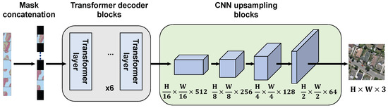
Figure 4. The structure of the MFM decoder.

In the masked concatenation operation, the unmasked sequence $E_x^m$ is concatenated with learnable vectors to restore its length to what it was before the random mask operation. Specifically, masked positions are replaced with learnable vectors, which are then decoded to produce predictions for the masked positions:

$$D_x^m=E_x^m+(N-M)\otimes V$$

(14)

$$V=\{v_1,v_2,v_3,\dots ,v_n\},n={\displaystyle \frac{H}{16}}\times {\displaystyle \frac{W}{16}}$$

(15)

where $E_x^m$ is the sequence after shared-weight encoding, M is the mask sequence, $N=\{1,1,1,\dots ,1\}$ is an all-1 one-dimensional sequence, V represents the sequence of learnable vector elements, with v being individual learnable vector elements, and $D_x^m$ is the sequence after concatenation.

The Transformer decoding part consists of six layers of Transformer units connected in series, forming an asymmetrical structure with the shared-weight encoder containing 12 layers. The asymmetrical structure is adopted because a symmetrical one may lead to a powerful decoder masking the lack of encoder representation by optimizing reconstruction ability, thereby limiting the quality of the encoder’s feature expression. The core goal of SSL is to pre-train an encoder with strong representation capabilities for application in downstream tasks. This design allows the encoder to learn more comprehensive representations, while the decoder primarily assists in this process. Additionally, the lightweight decoder reduces memory consumption and enhances algorithm utility in remote sensing applications. Specifically for remote sensing scenarios, remote sensing images often contain high-resolution details and complex spatial structures; a lightweight decoder prevents overfitting to reconstruction artifacts while encouraging the encoder to learn semantically meaningful features transferable to diverse downstream tasks such as semantic segmentation and object detection.

In the convolutional upsampling part, the 2D sequence output by the Transformer decoder is reshaped into a 3D feature map. Four convolutional upsampling units are then used to decode and predict restoration of the original image. Each unit comprises a $3\times 3$ convolution followed by bilinear interpolation upsampling. Through these convolutional upsampling stages, the feature map scales from $14\times 14$ to the final size of $224\times 224$. The final image prediction head adjusts the number of channels to 3 via a $1\times 1$ convolution.

3.7. Loss Function

We design loss functions for CLR and MFM branches. In the MFM branch, a random mask is applied to the feature map, and the original image is reconstructed through the shared-weight encoder and MFM decoder. For the loss calculation, L1 loss is computed between the reconstructed image predicted by the MFM decoder and the original image, considering only the masked region:

$$L1loss(x,y_{pre})={\displaystyle \frac{{\sum }_{i=1}^n|y_{pre,i}-x_i|\times {(N_0-M_0)}^T}{\mathrm{Sum}{(N_0-M_0)}^T}}$$

(16)

where $y_{pre}$ is the predicted image decoded by the MFM; x is the original image serving as ground truth n represents the number of images in a training batch; $N_0$ is a 3D matrix with all elements set to 1; $M_0$ is a 3D matrix reshaped from the mask sequence M with shape [H, W, 1] and values of 0 or 1; $N_0-M_0$ results in a matrix where elements that are 1 correspond to the masked blocks in the image; and Sum denotes the sum of elements in $N_0-M_0$, i.e., the number of masked blocks.

In the CLR branch, we use the widely adopted InfoNCE loss function. The core idea is to maximize similarity between pairs of positive samples (similar image pairs) while minimizing similarity between negative sample pairs (non-similar image pairs). This mechanism not only enhances the global representation capability and differentiation of features but also enables the model to understand image content at a higher level.

Specifically, in the CLR branch, each raw image $x_i$ goes through an image preprocessing stage, and two augmented images $x_{i_1}$ and $x_{i_2}$ are generated using two different data augmentation methods. These augmented images form image sample pairs $(x_{i_1},x_{i_2})$. These sample pairs are then processed by the feature extraction module, shared-weight encoder, and CLR decoder to obtain feature vectors $(z_{x_{i_1}},z_{x_{i_2}})$. The InfoNCE loss is calculated as follows:

$${\mathrm{InfoNCES}}_{(z_{x_{i_1}},z_{x_{i_2}})}=-\sum _{i=1}^{N}log\left({\displaystyle \frac{e^{\frac{\mathrm{sim}(z_{x_{i_1}},z_{x_{i_2}})}{\tau }}}{{\sum }_{j=1,[j\ne i]}^N\left[e^{\frac{\mathrm{sim}(z_{x_{i_1}},z_{x_{j_1}})}{\tau }}+e^{\frac{\mathrm{sim}(z_{x_{i_1}},z_{x_{j_2}})}{\tau }}\right]}}\right)$$

(17)

where N is the number of images in the batch; $z_{x_{i1}}$ and $z_{x_{i2}}$ represent feature vectors obtained from the CLR branch for two augmented images $(x_{i1},x_{i2})$ derived from the same original image $x_i$ using different data augmentation methods, i.e., positive sample pairs; $z_{x_{j1}}$ and $z_{x_{j2}}$ represent feature vectors obtained from the CLR branch for two augmented images generated from other images in the same batch that are different from the original image $x_i$, i.e., negative samples; $[j\ne i]$ is an indicator function ensuring that j cannot equal i; $\mathrm{sim}(·)$ represents the similarity function, calculated by a dot product in this paper; and $\tau$ is the temperature parameter that adjusts the sharpness of similarity distribution.

The calculation of total loss for the CMFM architecture combines two types of loss simultaneously. InfoNCE Loss emphasizes overall structural connections between different images, while L1 Loss focuses on local details within the same image. This multi-scale learning helps the model construct a more comprehensive and robust feature representation.

Since the two branches involved have distinct objectives and their loss values are of different magnitudes, direct addition may lead to one task’s gradient dominating, thereby affecting learning of the other. By weighting losses from both branches, we can balance their impact on gradient updates, ensuring that each task receives appropriate attention. The equation for total loss of CMFM is:

$$loss={\lambda }_1\times \mathrm{InfoNCELoss}+{\lambda }_2\times \mathrm{L}1\mathrm{loss}$$

(18)

where ${\lambda }_1$ and ${\lambda }_2$ are weight constants used to balance the two branches. In this paper, they are set to 0.1 and 1.0 respectively. Specifically, during training we observed that the contrastive learning loss (InfoNCE) typically ranges from 0.5 to 2.0, while the masked feature modeling loss (L1) operates within 0.05 to 0.2, exhibiting approximately a 10:1 magnitude difference. To balance the gradient contributions from both branches, we empirically selected ${\lambda }_1=0.1$ to reduce the weight of the InfoNCE loss and ${\lambda }_2=1.0$ to ensure adequate training of the reconstruction task. This 1:10 weight ratio effectively compensates for the magnitude difference in losses.

3.8. Model Evaluation

Feature representation ability of the model is evaluated using a downstream semantic segmentation task. We adopt a “self-pre-training” strategy: original images are used for training in the SSL stage, then the pre-trained parameters are loaded into the downstream task. Supervised training with a small number of labels follows, paying special attention to performance in small-sample scenarios.

The downstream task model integrates global modeling capabilities of Transformers with advantages of local information extraction from CNNs, constructing a semantic segmentation network that includes CNN-based feature extraction, a Transformer-based encoder, and CNN-based upsampling, as shown in Figure 5. The first two components leverage pre-trained parameters from CMFM and remain fixed during training to verify feature extraction ability developed during pre-training. Additionally, by incorporating skip connections between feature extraction and upsampling modules, multi-scale features are fused, reducing loss of spatial information and further enhancing semantic segmentation accuracy.

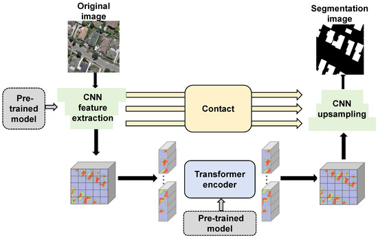
Figure 5. Network structure for the downstream semantic segmentation task.

4. Experiments and Results

4.1. Datasets

To verify the effectiveness of the proposed method, three public datasets were used for experiments:

• WHU Building Dataset (WHU) [34]: This dataset is primarily used for the building extraction task. The original images originate from the New Zealand Land Information Service website, with the shooting location in Christchurch. The spatial resolution of images is 0.3 m. The dataset comprises 8188 images of 512 × 512 pixels along with their corresponding ground truth. To conform to regular input sizes required by the ViT network, each 512 × 512 image was cropped into four non-overlapping images of 256 × 256 pixels. During self-supervised pre-training, we utilized images from the entire dataset. For downstream semantic segmentation tasks, images and their corresponding ground truth were divided into training, validation, and test sets, containing 18,940, 4140, and 9660 images, respectively.
• Massachusetts Buildings Dataset [35]: This dataset consists of 151 aerial images from the Boston area, each with a size of 1500 × 1500 pixels, covering an area of 2.25 square kilometers per image. The entire dataset collectively covers approximately 340 square kilometers. The dataset was constructed by randomly dividing data into a training set of 137 images, a test set of 10 images, and a validation set of 4 images. These images were then further cropped into smaller images of size 256 × 256 pixels.
• Gaofen Image Dataset (GID) [36]: This is a large-scale, high-resolution remote sensing image land cover dataset constructed using GF-2 satellite data in China. It is divided into two parts: the large-scale classification set (GID-5) and the fine land cover set (GID-15). In this study, we used GID-5, a dataset with five category labels, as a semantic segmentation dataset for downstream task fine-tuning. The GID-5 dataset includes five land cover categories: buildings, farmland, forests, grasslands, and water bodies. This dataset comprises 150 GF-2 satellite remote sensing images, each annotated at the pixel level. The training set consists of 120 images, while the validation set contains 30 images. Each GF-2 satellite remote sensing image measures 6800 × 7200 pixels and comes with corresponding labels. We cropped large images into 109,200 smaller images of 256 × 256 pixels and divided them into a training set (65,520 images), a validation set (21,840 images), and a test set (21,840 images) following a 6:2:2 ratio.

Some examples of images and their corresponding ground truth for the WHU dataset, the Massachusetts dataset, and the GID dataset are shown in Figure 6.

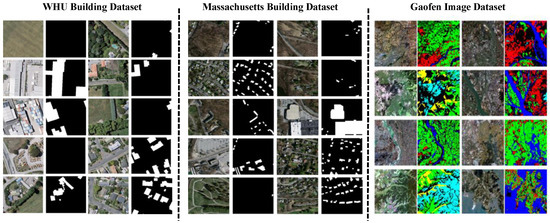
Figure 6. Some examples of images and their corresponding ground truth for the WHU dataset, the Massachusetts dataset, and the GID dataset.

4.2. Model Training Details

In terms of the model training environment, the hardware setup includes an Intel Core i9-10900K CPU @ 3.70 GHz (Intel Corporation, Santa Clara, CA, USA), 64 GB of memory, and an NVIDIA Tesla V100 32 GB graphics card (NVIDIA Corporation, Santa Clara, CA, USA). The software environment comprises Ubuntu, the PyTorch 1.10.2 deep learning framework, Python version 3.7, and CUDA version 10.2. Model training is divided into two stages: self-supervised pre-training of remote sensing images using the CMFM architecture, followed by fine-tuning for downstream semantic segmentation tasks.

Self-supervised pre-training: To ensure fairness and comparability of experimental results, we uniformly set the pre-training stage to 800 epochs for all self-supervised learning methods, maintaining consistency with established SSL approaches (MAE, BEiT, and other methods typically employ 800–1600 epochs). This configuration ensures adequate convergence for CMFM while guaranteeing sufficient training for all comparative methods. All models were initialized with ImageNet21k pre-trained parameters to provide a consistent starting point. We adopt this initialization strategy for two reasons: First, it aligns with common practice in the remote sensing SSL community, where researchers typically leverage natural image pre-training to accelerate convergence and improve feature quality, especially given the limited scale of available remote sensing datasets. Second, using ImageNet21k initialization ensures fair comparison with baseline methods (e.g., BEiT, MAE, data2vec), which were originally designed with such initialization and may not converge effectively from random initialization within practical training budgets. This approach allows us to focus on evaluating the architectural contributions of CMFM rather than confounding results with optimization difficulties. The optimization was performed using AdamW optimizer with beta parameters set to (0.9, 0.999), learning rate of 0.001, and weight decay of $1\times {10}^{-8}$. The temperature parameter $\tau$ for the InfoNCE loss in Equation (17) was configured to 0.7. Data augmentation techniques comprised random cropping, random flipping, and color jittering, scaling the input image dimensions to $224\times 224\times 3$ and effectively doubling the training dataset size. The batch size was configured to 64. Upon completion of the pre-training phase, we exclusively preserved the network parameters from the convolutional feature extraction module and the shared-weight encoder of the pre-trained model. These learned parameters were subsequently transferred to downstream tasks for fine-tuning evaluation.

Fine-tuning of downstream semantic segmentation: The fine-tuning procedure for downstream tasks serves as the primary mechanism for validating the quality of model parameters acquired through self-supervised learning. The semantic segmentation network architecture comprises three fundamental components: a CNN-based feature extraction module, a Transformer-based encoder, and a CNN-based decoder. The parameters of both the CNN-based feature extraction module and the Transformer-based encoder were initialized using self-supervised pre-trained parameters derived from the CMFM architecture, while the CNN-based decoder parameters underwent random initialization. To rigorously assess feature extraction capabilities of our CMFM methodology, parameters of the CNN-based feature extraction module and the Transformer-based encoder remained frozen during training, with only the CNN-based decoder parameters being optimized.

Concerning hyperparameter configuration, we employed a training regimen of 200 epochs for both the ablation study fine-tuning phase and comparative experiments. The convergence criterion was established such that when the validation set IoU or mIoU improvement remained below 0.2% over 10 consecutive epochs, the model was considered to have achieved convergence. Throughout the entire training process, we continuously monitored validation set performance and automatically preserved model parameters yielding the highest validation IoU or mIoU as final results. Optimization was conducted using Adam optimizer with beta parameters configured to (0.9, 0.999), learning rate set to 0.001, and weight decay of $1\times {10}^{-8}$. Input image dimensions were standardized to $224\times 224\times 3$. During data loading operations, batch size was configured to 196. Systematic monitoring of model convergence behavior was implemented across all ablation experiments. Since this phase specifically targets validation of self-supervised learning quality and evaluation of autoencoder pre-training parameters within the CMFM architecture, data augmentation techniques were deliberately omitted from the data loading pipeline.

4.3. Metrics

The metrics used in this paper include Intersection over Union (IoU) and mean Intersection over Union (mIoU).

IoU measures the overlap between predicted results and ground truth. It is calculated using the following equation:

$$\mathrm{IoU}={\displaystyle \frac{TP}{TP+FP+FN}}$$

(19)

where $TP$ represents true positives, $FP$ represents false positives, and $FN$ represents false negatives.

In the context of the GID-5 dataset, IoU serves as the accuracy index for semantic segmentation of each category. To evaluate overall semantic segmentation accuracy across all categories, mean Intersection over Union (mIoU) is utilized. mIoU is the average of IoU values for all categories and is calculated as follows:

$$\mathrm{mIoU}={\displaystyle \frac{1}{k}}\sum _{i=1}^k{\displaystyle \frac{T{P}_i}{F{N}_i+F{P}_i+T{P}_i}}$$

(20)

where k is the number of all categories except the background, and $T{P}_i$, $F{N}_i$, and $F{P}_i$ represent the true positives, false negatives, and false positives for the i-th category, respectively.

4.4. Ablation Study

Ablation studies were performed on the WHU dataset to evaluate the effectiveness of the different components of our framework in this section. To ensure the fairness and comparability of the experimental results, the training parameter settings for the CMFM model and the fine-tuning for the downstream semantic segmentation task were strictly carried out according to the training details described in Section “Model Training Details”. For the accuracy evaluation, IoU was selected as the primary metric. The following sections will explore the performance comparisons of different data preprocessing strategies, mask ratios, decoder depths, and branches within the CMFM architecture.

1.

Different Data Preprocessing Strategies

To evaluate the impact of different preprocessing methods on the performance of the CMFM framework, this study employed four data augmentation strategies: “random cropping”, “random cropping + color jitter”, “random cropping + random flipping”, and “random cropping + random flipping + color jitter”. The experimental results are shown in Table 1. Table 1 indicates that the best performance was achieved using a combination of color jitter, random cropping, and random flipping. The contrastive learning task benefits from a certain level of data augmentation to enhance the distinction between the two views of an image. Specifically, color jitter improves the model’s ability to distinguish changes under different lighting conditions, while random cropping and flipping enhance spatial perception by altering the spatial layout of images. This data augmentation strategy increases the diversity of input images, taking into account both the mask feature strategy and the contrastive learning strategy. It better simulates the variations in remote sensing images under complex conditions, thereby promoting the model to learn more robust and generalizable feature representations. Surprisingly, our approach performs well even without extensive data augmentation (limited to random cropping, with no flipping or color jitter). This is because, in MFM tasks, the role of data augmentation is primarily achieved through random masks, which vary with each iteration, thereby generating new training samples regardless of traditional augmentation techniques.

Table 1. Comparison of Semantic Segmentation Results of Different Preprocessing Strategies on the WHU Dataset (Unit: %). Bold values indicate the best results.

Different Preprocessing Strategies	IoU
Random cropping	86.32
Random cropping + color jitter	86.85
Random cropping + random flipping	87.12
Random cropping + random flipping + color jitter	87.94

2.

Different Mask Ratios

In this investigation, we employed seven distinct fixed mask ratios (15%, 25%, 40%, 50%, 65%, 75%, 85%), along with a random mask ratio ranging from 25% to 80% to systematically assess the sensitivity of CMFM to mask ratio hyperparameters. The experimental results are presented in Table 2. As demonstrated in Table 2, CMFM exhibits moderate sensitivity to mask ratio configurations. Mask ratios between 25% and 65% yield optimal performance (IoU: 85.87–86.45%), while extreme ratios (15% and 85%) lead to performance degradation. Lower mask ratios provide insufficient challenges for meaningful representation learning, whereas higher ratios create excessively difficult reconstruction tasks. Our random mask ratio strategy achieved superior performance (IoU: 87.94%), with its advantages stemming from three core mechanisms: First, the dynamic difficulty adjustment mechanism provides the model with multi-granularity reconstruction tasks ranging from low to high difficulty through varying mask ratios during training, enabling the model to progressively enhance learning capabilities across different masking levels while avoiding the learning limitations that may arise from single-difficulty levels. Second, the anti-overfitting capability significantly enhances model generalization and stability by preventing excessive model dependence on specific masking patterns through diverse masking modes. Finally, the diversified feature learning mechanism facilitates the model’s acquisition of more adaptive feature representations across different scales, making it better suited for the complex spatial structures of remote sensing imagery.

Table 2. Comparison of Semantic Segmentation Results of Different Mask Ratios on WHU Dataset (Unit: %). Bold values indicate the best results.

Mask Ratio	IoU
15%	85.23
25%	86.21
40%	86.45
50%	86.24
65%	85.87
75%	85.34
85%	83.92
Random mask ratio	87.94

3.

Different Decoder Depths

To evaluate the performance of the MFM decoder at different depths, we conducted experiments with the MFM decoder at various depth levels (i.e., different numbers of Transformer blocks). The experimental results are shown in Table 3. It can be seen that when both the decoder and the shared-weight encoder are configured with 12 layers, this setup not only prolongs the training time but also weakens the performance of the semantic segmentation task. This suggests that too many decoder layers may interfere with the feature extraction capabilities of the encoder, which, in turn, affects its performance in downstream tasks. By reducing the decoder to 6 layers, we found that the IoU reaches its highest value of 87.94%, striking the sweet spot between efficiency and performance. When further reduced to 4 layers, however, the model did not achieve the expected performance, despite its simpler structure. This is because a sufficiently deep decoder is crucial for reconstructing images, allowing latent features to remain at a more abstract level, which aids in improving recognition performance. Thus, the importance of maintaining a certain depth is confirmed. It is worth noting that when the decoder depth is set to the optimal depth of 8 layers, as in MAE, although the IoU reaches 87.92%—nearly matching the performance of the 6-layer decoder—this does not bring significant performance improvements and instead reduces computational efficiency. Based on these considerations, 6 layers are determined to be the optimal depth choice for the MFM decoder, ensuring both high performance and efficient use of computing resources.

Table 3. Comparison of Semantic Segmentation Results with Different Decoder Depths (Unit: %). Bold values indicate the best results.

Decoder Depths	IoU	Hours
1	86.90	156.33
4	87.61	159.29
6	87.94	162.58
8	87.92	167.78
12	86.86	184.52

4.

Different Branches of the CMFM Architecture

To evaluate the performance of different branches of the CMFM architecture in limited sample tasks, we randomly selected samples from the WHU dataset at ratios of 5%, 10%, 20%, 40%, 60%, and 100% to test the performance of the MFM branch, the CLR branch, and their combinations. The details are as follows:

• TransUnet: The baseline network has the same encoder structure as our model and initializes with the pre-trained R50-ViT-B_16 model on ImageNet21k for fully supervised training.
• MFM: Self-supervised training using only the MFM branch and a random mask ratio strategy.
• CLR: Self-supervised training using only the CLR branch.
• CMFM: Self-supervised training using both the MFM and CLR branches.

With these settings, we comprehensively evaluated the effectiveness of each branch and its combination under different sample sizes, particularly focusing on performance and advantages under small sample conditions. The experimental results are shown in Table 4, where the IoU index for the semantic segmentation task was selected as the accuracy metric.

Table 4. Comparison of the Performance of Different Branches of the CMFM Architecture on the WHU Dataset (Unit: %). Bold values indicate the best results.

Architecture	5%	10%	20%	40%	60%	100%
TransUnet (baseline)	58.55	72.47	78.65	80.86	82.59	85.66
MFM	75.39	79.05	80.20	82.32	82.85	83.59
CLR	80.07	81.83	83.80	85.31	86.40	87.17
CMFM	82.70	83.59	84.67	86.05	86.51	87.94

The ablation experimental results presented in Table 4 demonstrate that the proposed CMFM method consistently outperforms the baseline TransUnet network across all sample proportions in terms of IoU evaluation metrics. Particularly under limited sample conditions, the self-supervised pre-trained MFM, CLR, and CMFM models all surpassed the baseline TransUnet, with CMFM achieving an IoU of 82.70% when the sample size was 5%. However, the MFM branch alone yielded only 75.39%, indicating a significant performance disadvantage when constrained to learning through masking patterns exclusively, rather than achieving genuine semantic understanding. Further experimental evidence reveals that the CLR branch consistently outperformed the MFM branch across all experimental conditions, while the dual-branch CMFM architecture achieved optimal overall performance, substantially surpassing any single-branch configuration. When utilizing 100% of the dataset, this performance differential becomes more pronounced: MFM’s performance (83.59%) falls below that of the TransUnet baseline (85.66%), whereas both the CLR branch and CMFM model demonstrate exceptional performance, significantly outperforming the standalone MFM model.

The experiments additionally reveal a critical phenomenon: the fusion advantage of dual branches diminishes as dataset scale increases. Specifically, compared to CLR alone, CMFM achieved a 2.63% improvement at 5% sample size, but only a 0.77% improvement at 100% sample size. This phenomenon reflects the inherent limitations of masked reconstruction tasks relative to contrastive discriminative learning. Despite these constraints, CMFM successfully realizes superior feature quality in downstream semantic segmentation tasks by synergistically combining the fine-grained local details acquired through MFM with the global structural information captured by CLR. This complementary architectural design not only significantly enhances the model’s generalization capabilities in small-sample scenarios but also demonstrates exceptional performance on large-scale datasets, conclusively validating the effectiveness of fusing MFM and CLR branch strategies.

5.

Component Contribution Analysis of CNN+Transformer Hybrid Architecture

To assess individual component contributions within our CNN+Transformer hybrid architecture, we evaluate four configurations: CNN (ResNet50 with 7 × 7 feature maps), Transformer (Vision Transformer), CNN+Transformer (7 × 7) (ResNet50 7 × 7 + ViT), and CNN+Transformer (14 × 14) (our proposed architecture). Results are presented in Table 5.

Table 5. Component Contribution Analysis on WHU Dataset (Unit: %). Bold values indicate the best results.

Method	Architecture	IoU (%)	Accuracy (%)	Precision (%)	Recall (%)	F1-Score
CNN	ResNet50 (7 × 7)	80.31	97.10	85.54	92.92	89.08
Transformer	ViT	80.47	97.63	89.66	88.70	89.18
CNN+Transformer	ResNet50 (7 × 7) + ViT	84.64	99.12	92.44	90.94	91.68
CNN+Transformer	ResNet50 (14 × 14) + ViT	85.40	98.28	92.87	91.40	92.13

Table 5 demonstrates that our CNN+Transformer (14 × 14) hybrid architecture substantially outperforms single-component approaches, achieving 5.09% and 4.93% IoU improvements over CNN and Transformer baselines, respectively. Critically, the 14 × 14 configuration surpasses the 7 × 7 variant by 0.76% IoU, confirming the importance of spatial resolution preservation for remote sensing applications. The CNN component excels at extracting local fine-grained features (building boundaries, textures), while the Transformer captures global spatial relationships and contextual dependencies. This synergy enables the hybrid architecture to balance local detail preservation with long-range dependency modeling, achieving superior semantic understanding compared to individual components.

4.5. Comparative Experiments

To further verify the effectiveness of the proposed method, we conducted comparative experiments with the following six state-of-the-art SSL algorithms. A brief introduction to these algorithms is as follows:

• BEiT [16]: BEiT is the first masked image modeling (MIM) SSL algorithm based on Transformer architecture. It learns image representations by masking parts of the image and predicting the content of those regions.
• SimMIM [22]: Building on BEiT, SimMIM simplifies the masked image modeling method by directly reconstructing the original pixels. It omits the encoder–decoder structure and uses a linear projection layer for reconstruction.
• MAE [19]: MAE introduces an asymmetric encoder–decoder architecture that encodes only unmasked image blocks. This approach allows for a higher mask ratio, which not only significantly reduces computational effort but also forces the model to learn richer global contextual information.
• CAE [23]: CAE is a masked image modeling method that strictly separates the representation learning role from the pretext task completion role. CAE learns a more comprehensive image representation by predicting and reconstructing the occluded image blocks in the encoded representation space.
• MFM [10]: MFM is a masked feature modeling method specifically designed for hybrid CNN+Transformer architectures, enabling effective feature learning across different architectural components.
• data2vec [37]: data2vec represents the first unified cross-modal self-supervised learning framework employing a teacher–student architecture for speech, vision, and text processing. Unlike traditional discrete token prediction, it predicts continuous contextualized representations, though limited to single masking strategies.

To ensure objectivity and fairness in the evaluation, we implemented all comparison methods under identical training conditions: (1) Backbone architecture: All methods employ ResNet50 for feature extraction followed by a 12-layer ViT-B Transformer encoder, initialized with ImageNet21k pre-trained parameters. (2) Pre-training configuration: All methods are trained for 800 epochs with batch size 64, using AdamW optimizer (learning rate 0.001, weight decay $1\times {10}^{-8}$). (3) Data augmentation: All methods use the same augmentation pipeline (random cropping to $224\times 224$, random horizontal flipping, color jittering), with method-specific mask ratios as recommended by the original authors. (4) Training datasets: All methods are pre-trained on the complete dataset (training + validation + test sets) for each benchmark. (5) Downstream evaluation: All methods use the same decoder architecture (convolutional upsampling-based) with frozen encoder parameters during fine-tuning to isolate the evaluation of pre-trained representations.

Comparative experiments were conducted on three semantic segmentation datasets: WHU, Massachusetts, and GID. First, we performed self-supervised pre-training using all raw images from each dataset, including the training, validation, and testing sets. Subsequently, in the downstream semantic segmentation task, we used training sets with different sample sizes for fine-tuning and statistically evaluated the model accuracy. For accuracy evaluation, the primary reference metric is the IoU index. With these settings, we were able to comprehensively evaluate the performance of the proposed method across different datasets and sample sizes under controlled and transparent experimental conditions.

1.

Comparison on the WHU Dataset

To evaluate the effectiveness of our method, we conducted comparative experiments on the WHU dataset using different training sample sizes: 5%, 10%, 20%, 40%, 60%, and 100%. During the experiments, we utilized all raw images from the dataset—including those from the training, validation, and test sets—for self-supervised pre-training. Subsequently, we fine-tuned the pre-trained model using training sets with varying sample sizes. The semantic segmentation results of different methods on the WHU dataset with varying sample sizes are compared in Table 6.

Table 6. Comparison of Semantic Segmentation Results of Different Methods on the WHU Dataset with Varying Sample Sizes (Unit: %). Bold values indicate the best results.

Model	5%	10%	20%	40%	60%	100%
BEiT (baseline)	66.23	72.33	73.84	76.44	77.23	78.02
SimMIM	71.62	74.68	75.75	76.06	77.28	79.16
MAE	71.84	75.53	77.48	78.27	79.30	80.87
CAE	73.01	77.16	78.56	79.05	80.81	81.86
data2vec	67.04	72.42	76.22	80.90	82.86	85.09
MFM	75.39	79.05	80.20	82.32	82.85	83.59
CMFM (ours)	82.70	83.59	84.67	86.05	86.51	87.94

As demonstrated in Table 6, our proposed method substantially outperforms all competing approaches across varying sample sizes. At 100% data utilization, CMFM achieves a 9.92% IoU improvement over the BEiT baseline. Performance gains are particularly pronounced in small-sample scenarios (5% and 10% data), where IoU increases by 16.47% relative to BEiT. Further analysis reveals SimMIM consistently surpasses BEiT across all data scales, validating direct pixel reconstruction effectiveness. MAE attains 80.87% IoU at 100% sample size, exceeding SimMIM by 1.71% through its asymmetric encoder–decoder architecture and elevated masking ratios that facilitate richer global contextual learning. CAE achieves 73.01% and 81.86% IoU at 5% and 100% sample sizes respectively, surpassing MAE and demonstrating encoder representation and alignment mechanism efficacy. data2vec exhibits competitive performance, achieving 85.09% IoU at 100% data scale—a 4.22% improvement over MAE, though showing limited small-sample performance with only 67.04% IoU at 5% data scale, reflecting unified framework limitations in domain-specific optimization. MFM produces suboptimal results across 5–40% data ranges, highlighting the benefits of CNN–Transformer hybrid architectures for small-sample scenarios. Remarkably, our CMFM method excels in small-sample conditions, achieving 82.70% IoU at 5% data scale—a 15.66% improvement over data2vec. This success stems from CMFM’s integration of MFM strengths with contrastive learning mechanisms, capturing both global image context and discriminative inter-image features, significantly enhancing performance under limited training conditions.

To further compare the performance of seven methods at 5% and 100% sample scales, we visualized semantic segmentation results from different approaches on the WHU building dataset, as shown in Figure 7. When fine-tuned with only 5% training data, the other six methods (SimMIM, BEiT, MAE, CAE, data2vec, MFM) exhibit significantly higher false positive and false negative rates compared to CMFM. Row one demonstrates that SimMIM, BEiT, MAE, and MFM generate false positive and negative regions when identifying small building clusters, while CMFM exhibits minimal false positive areas. Row two shows that in dense small building complexes, SimMIM, BEiT, MAE, and MFM produce more severe errors, with BEiT erroneously connecting separate buildings and SimMIM, MAE, and CAE generating internal voids in small buildings, whereas CMFM achieves superior structural identification. Row three reveals that SimMIM, BEiT, MAE, and data2vec encounter severe false negative problems when detecting individual buildings, while CAE demonstrates relative stability but still exhibits partial internal false negatives, and MFM and CMFM perform effectively in this task. Additionally, CMFM predicts building edges with superior sharpness and closer ground truth alignment, demonstrating exceptional local detail prediction capability. At 100% training data utilization, all methods achieve significant accuracy improvements; however, CMFM consistently maintains optimal performance among the seven approaches, further validating its superiority and robustness.

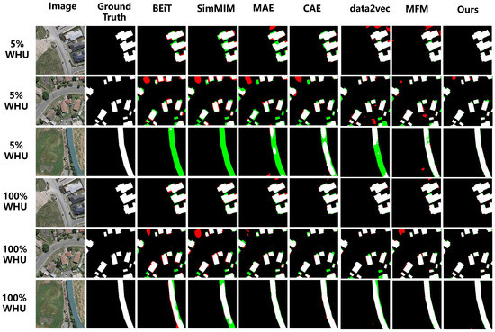
Figure 7. Visualization of Semantic Segmentation Results on the WHU Building Dataset: White—True Positives; Black—True Negatives; Red—False Positives; Green—False Negatives.

2.

Comparison on the Massachusetts Dataset

To further evaluate the effectiveness of our method on smaller datasets, we conducted comparative experiments using different sample sizes from the Massachusetts Buildings (Massa) dataset, with the results shown in Table 7.

Table 7. Comparison of Semantic Segmentation Results of Different Methods on the Massachusetts Dataset with Varying Sample Sizes (Unit: %). Bold values indicate the best results.

Model	5%	10%	20%	40%	60%	100%
BEiT (baseline)	37.69	40.56	42.66	47.08	47.55	47.93
SimMIM	35.50	39.17	42.28	42.29	43.33	44.29
MAE	37.70	39.81	41.70	45.98	47.20	47.96
CAE	40.36	42.59	46.37	48.28	50.43	50.91
data2vec	42.72	50.58	51.73	55.49	56.79	58.88
MFM	42.49	45.67	47.79	50.86	51.89	53.48
CMFM (ours)	51.51	53.88	56.98	59.74	61.59	62.96

As demonstrated in Table 7, the proposed method substantially outperforms all competing approaches on the Massachusetts dataset. At 100% data utilization, CMFM achieves a 13.82% IoU improvement over the BEiT baseline. At 5% data scale, IoU increases by 13.66% relative to baseline BEiT, confirming our method’s superiority in small-sample scenarios. Further analysis reveals SimMIM underperforms BEiT across all data scales, likely reflecting difficulties in effectively learning discriminative feature representations on compact small datasets. MAE exhibits performance comparable to BEiT with slight inferiority at multiple scales, indicating challenges in acquiring sufficient discriminative features from high-similarity images. Conversely, CAE demonstrates marginal improvements, potentially attributed to its contrastive learning mechanism integration. data2vec achieves competitive performance, reaching 58.88% IoU at 100% data scale and 42.72% at 5% data scale, though showing limitations in complex spatial structure understanding reflecting unified framework constraints in domain-specific optimization. MFM achieves superior performance across all data scales, reaching 53.48% IoU at 100% data scale (a 5.55% improvement over baseline BEiT (47.93%)), and 42.49% IoU at 5% scenarios, comparable to data2vec but significantly outperforming SimMIM (35.50%) and MAE (37.70%), confirming mixed architectures’ enhanced robustness under data-scarce conditions.

Remarkably, our CMFM method achieves optimal performance on the Massachusetts dataset, reaching 62.96% at 100% data scale (a 4.08% improvement over data2vec) and 51.51% at 5% data scale (an 8.79% improvement over data2vec). This success stems from dual-branch structured advantages under multi-modal scenarios, where contrastive learning enhances cross-image building and target distribution understanding, effectively addressing high-similarity challenges unique to the Massachusetts dataset. Notably, CMFM achieves maximum absolute performance gains compared to other methods, reaching 87.94% on WHU versus 62.96% on Massachusetts (a substantial 24.98% difference). This differential demonstrates CMFM’s sensitivity to image resolution and contrast, where Massachusetts dataset’s low resolution and high similarity severely constrain pixel-level reconstruction effectiveness.

To further compare the performance of the seven methods at 5% and 100% sample sizes, we visualized the semantic segmentation results from different methods on the Massachusetts building dataset, as shown in Figure 8. The data reveals that when fine-tuning with only 5% training data, our CMFM exhibits superior performance with lower false positive and false negative rates. Specifically, when using only 5% training data for fine-tuning (as shown in the first row of Figure 8), BEiT, CAE, MAE, and data2vec demonstrate higher false positive rates, incorrectly labeling non-target areas as buildings while exhibiting significant connectivity errors by erroneously connecting separate buildings, stemming from inherent limitations of discrete token prediction mechanisms in processing continuous spatial structures. Conversely, SimMIM shows high false negative rates, failing to correctly identify existing buildings. In contrast, MFM and our CMFM method more effectively identify building features while maintaining lower false positive and false negative rates. Notably, CMFM provides clearer edges for small buildings, demonstrating its unique advantage in detail processing. When training data increases to 100%, all methods achieve significant accuracy improvements, yet CMFM maintains its leading position among the seven approaches. Particularly in densely populated areas (as shown in Figure 8), other methods still produce numerous false positives and false negatives, especially when processing sharp building corners. Conversely, CMFM accurately captures complex inter-building structures in low-resolution and high-similarity images, further validating its effective performance under low sampling rates and small dataset conditions. CMFM performs exceptionally well on targets with complex geometric structures such as buildings, benefiting from its CNN+Transformer architecture’s effective modeling capability for multi-scale geometric features.

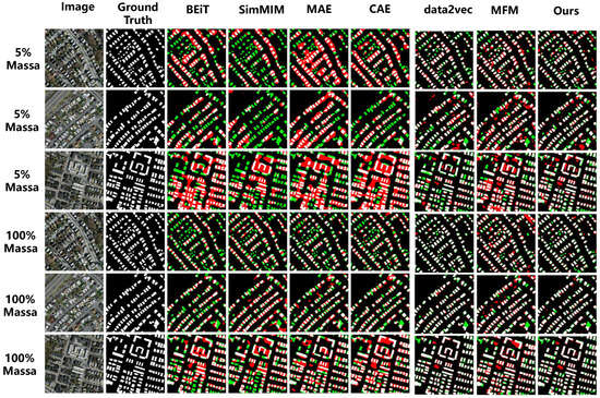
Figure 8. Visualization of Semantic Segmentation Results on the Massachusetts Building Dataset: White—True Positives; Black—True Negatives; Red—False Positives; Green—False Negatives.

3.

Comparison on the GID Dataset

To further verify the effectiveness of our method on large-scale, multi-classification datasets of high-resolution remote sensing images, we conducted comparative experiments using the GID-5 dataset, which encompasses five typical land cover types. The experimental results are shown in Table 8.

Table 8. Comparison of Semantic Segmentation Results of Different Methods on the GID Dataset (Unit: %). Bold values indicate the best results for each category.

Model	IoU of Built-Up	IoU of Farmland	IoU of Forest	IoU of Meadow	IoU of Water	mIoU
BEiT (baseline)	84.27	68.61	66.80	59.91	66.22	69.16
SimMIM	84.99	70.56	69.01	61.69	68.97	71.03
MAE	85.72	73.03	69.10	61.38	68.44	71.53
CAE	86.31	73.06	66.67	62.67	69.35	71.61
data2vec	86.71	74.44	65.48	62.20	71.38	71.20
MFM	86.42	73.13	69.09	64.13	68.88	72.33
CMFM (ours)	85.49	76.43	67.00	62.38	70.34	72.59

Table 8 compares the semantic segmentation results of different methods on the GID dataset, revealing distinct performance patterns across the seven approaches. On the GID-5 dataset, due to the relatively large sample size, the mIoU differences between methods are smaller than those observed in other semantic segmentation datasets. BEiT baseline achieves balanced but modest performance across all categories (mIoU 69.16%) with particular weakness in meadow segmentation (59.91%), while SimMIM shows improvements over BEiT in most categories (mIoU 71.03%), demonstrating the effectiveness of simplified masking strategies in multi-class scenarios. MAE excels in forest segmentation (69.1%, highest among all methods) due to its high masking ratio facilitating texture pattern learning, though it struggles with water body identification. CAE achieves the highest built-up IoU (86.31%) through its contrastive alignment mechanism, particularly effective for structured targets, while maintaining competitive farmland performance. data2vec exhibits strong performance in farmland (74.44%) and water categories (71.38%) through its continuous representation learning, though forest segmentation remains challenging (65.48%). MFM demonstrates exceptional meadow segmentation capabilities (64.13%, highest) and competitive built-up performance (86.42%), highlighting the CNN+Transformer architecture’s effectiveness for diverse land cover types. Our CMFM achieves the highest mIoU (72.59%) by excelling in farmland (76.43%) and water segmentation (70.34%), but in-depth analysis of experimental data also reveals CMFM’s applicability boundaries under specific scenarios. Notably challenging is fine-grained structure segmentation, where CMFM achieves an IoU of 67.00% for forest categories, showing performance gaps compared to built-up (85.49%) and farmland (76.43%). Through detailed analysis of the first row in Figure 9, we observe that CMFM exhibits relatively smoothed characteristics in complex textured regions like forests, reflecting the mechanism of the masked modeling branch prioritizing continuous texture pattern reconstruction while facing technical challenges when processing high-frequency details such as tree edges. Further analysis reveals CMFM’s specific challenges in handling category imbalance scenarios, with relatively lower performance in meadow categories (IoU 62.38%), which typically cover smaller areas and share spectral similarities with farmland, while MFM demonstrates clear advantages in this category (64.13% vs. 62.38%), indicating that masked feature modeling possesses unique detail capture capabilities when processing small-area, spectrally similar land objects, providing important insights for optimizing dual-branch architecture coordination mechanisms in complex scenarios.

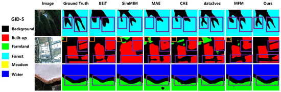
Figure 9. Visual comparison of semantic segmentation results on the GID-5 Dataset. The orange box indicates incorrect segmentation areas, while the purple box highlights regions showcasing the comparative performance between different methods.

The visual comparison of semantic segmentation results on the GID-5 Dataset is shown in Figure 9. Figure 9 demonstrates that our CMFM model exhibits superior performance compared to other methods, significantly reducing false and missed detections. Notably, in the segmentation of forest regions (first row of Figure 9), BEiT, CAE, MAE, and MFM all suffer from varying degrees of detail loss in fine branch structures. While data2vec performs moderately, it still exhibits slight boundary over-smoothing. In contrast, CMFM effectively preserves intricate texture patterns and delivers the best detection performance. In terms of building area segmentation (second row of Figure 9), BEiT, CAE, and MAE struggled with gaps and sharp parts of buildings. In contrast, CMFM not only accurately segments buildings but also retains building boundary details well, with segmentation accuracy significantly better than other methods. Additionally, for the segmentation of water and farmland (third row of Figure 9), CMFM performed exceptionally well. Its segmentation boundaries closely matched the real labels, especially in edge details (as highlighted by the purple boxed areas). These findings further demonstrate the effectiveness and robustness of CMFM in handling complex scenarios, even on large-scale datasets.

5. Conclusions

In this study, we propose a self-supervised learning framework (CMFM) that integrates contrastive learning and masked feature modeling strategies, aiming to effectively address the challenges posed by small-sample datasets in remote sensing image processing. By incorporating the contrastive learning branch of the SimCLR framework and an autoencoder branch based on masked feature modeling, the proposed architecture not only enhances the representation of global features but also improves the accuracy of local details, thereby achieving an effective combination of global and local features. Moreover, the application of a CNN+Transformer hybrid architecture further boosts the model’s performance in downstream pixel-wise tasks such as semantic segmentation.

To verify the effectiveness of our framework, we compared it with existing mainstream methods on three well-known open-source datasets. The extensive experiments show that CMFM not only achieves higher accuracy across multiple datasets but also maintains stable high performance at different data volumes. Especially in small-sample scenarios (such as 5% sample size), the IoU of CMFM is significantly higher than that of other methods, demonstrating its superior accuracy and stronger feature extraction ability under conditions of limited samples. Furthermore, we conducted ablation studies from four aspects to verify the effectiveness of different modules: data preprocessing strategy, mask ratio setting, decoder depth, and branch performance. The experimental results indicate that all components of our CMFM are effective, and they work synergistically to enhance the overall performance of the framework.

While CMFM shows promising performance in building extraction and land cover classification tasks, there remain some limitations worth noting. The validation scope remains confined to datasets with well-defined object boundaries (WHU, Massachusetts, and GID), and generalizability to other scenarios—such as change detection, small object detection, or hyperspectral/SAR imagery—requires further investigation. Future work should focus on three key directions: (1) developing adaptive dual-branch weight adjustment mechanisms through meta-learning or reinforcement learning to optimize task-specific performance; (2) extending the framework to handle multi-spectral and hyperspectral data with specialized architectural modifications; and (3) validating effectiveness across diverse remote sensing tasks and exploring cross-modal SSL by integrating optical-SAR imagery or temporal sequences for video-based analysis. These extensions would comprehensively assess CMFM’s applicability boundaries and enhance its robustness for real-world operational scenarios.

References

- Ma, L.; Liu, Y.; Zhang, X.; Ye, Y.; Yin, G.; Johnson, B.A. Deep learning in remote sensing applications: A meta-analysis and review. ISPRS J. Photogramm. Remote Sens. 2019, 152, 166–177. [Google Scholar] [CrossRef]
- He, K.; Zhang, X.; Ren, S.; Sun, J. Deep Residual Learning for Image Recognition. In Proceedings of the IEEE Conference on Computer Vision and Pattern Recognition (CVPR), Las Vegas, NV, USA, 27–30 June 2016; pp. 770–778. [Google Scholar]
- Dosovitskiy, A.; Beyer, L.; Kolesnikov, A.; Weissenborn, D.; Zhai, X.; Unterthiner, T.; Dehghani, M.; Minderer, M.; Heigold, G.; Gelly, S.; et al. An Image is Worth 16 × 16 Words: Transformers for Image Recognition at Scale. In Proceedings of the International Conference on Learning Representations (ICLR), Virtual Event, 3–7 May 2021. [Google Scholar]
- Li, X.; Shi, D.; Diao, X.; Xu, H.; Hou, M.; Liu, H.; Lu, Y.; Yang, J.; Wang, H.; Xu, Q.; et al. SCL-MLNet: Boosting Few-Shot Remote Sensing Scene Classification via Self-Supervised Contrastive Learning. IEEE Trans. Geosci. Remote Sens. 2022, 60, 5801112. [Google Scholar] [CrossRef]
- Zhang, Y.; Li, P.; Wang, X.; Su, H.; Jiang, J. Agricultural Land Cover Classification Using Multi-temporal Satellite Imagery: A Deep Learning Approach. Comput. Electron. Agric. 2022, 198, 107079. [Google Scholar]
- Zhou, S.; Liu, K.; Wang, J.; Li, L.; Yang, W. Small Object Detection in High-Resolution Remote Sensing Images: Current Status and Future Directions. ISPRS J. Photogramm. Remote Sens. 2022, 189, 243–259. [Google Scholar]
- Wang, J.; Chen, L.; Ma, Y.; Zhang, X.; Liu, H. Systematic Analysis of Masked Autoencoder Biases in Remote Sensing Applications. IEEE J. Sel. Top. Appl. Earth Obs. Remote Sens. 2023, 16, 8934–8947. [Google Scholar]
- Chen, X.; He, K. Exploring Simple Siamese Representation Learning. In Proceedings of the IEEE/CVF Conference on Computer Vision and Pattern Recognition (CVPR), Virtual Event, 19–25 June 2021; pp. 15750–15758. [Google Scholar]
- Zhang, H.; Cisse, M.; Dauphin, Y.; Lopez-Paz, D. mixup: Beyond Empirical Risk Minimization. In Proceedings of the International Conference on Learning Representations (ICLR), Vancouver, BC, Canada, 30 April–3 May 2018. [Google Scholar]
- Pang, S.; Xiang, J.; Zuo, Z.; Zhou, D. Masked Feature Modeling for Generative Self-Supervised Representation Learning of High-Resolution Remote Sensing Images. IEEE J. Sel. Top. Appl. Earth Obs. Remote Sens. 2024, 17, 7890–7905. [Google Scholar] [CrossRef]
- Chen, T.; Kornblith, S.; Norouzi, M.; Hinton, G. A Simple Framework for Contrastive Learning of Visual Representations. In Proceedings of the 37th International Conference on Machine Learning (ICML), Virtual Event, 13–18 July 2020; pp. 1597–1607. [Google Scholar]
- He, K.; Fan, H.; Wu, Y.; Xie, S.; Girshick, R. Momentum Contrast for Unsupervised Visual Representation Learning. In Proceedings of the IEEE/CVF Conference on Computer Vision and Pattern Recognition (CVPR), Seattle, WA, USA, 13–19 June 2020; pp. 9729–9738. [Google Scholar]
- Grill, J.B.; Strub, F.; Altché, F.; Tallec, C.; Richemond, P.H.; Buchatskaya, E.; Doersch, C.; Pires, B.A.; Guo, Z.D.; Azar, M.G.; et al. Bootstrap Your Own Latent: A New Approach to Self-Supervised Learning. In Proceedings of the Advances in Neural Information Processing Systems (NeurIPS), Virtual Event, 6–12 December 2020; Volume 33, pp. 21271–21284. [Google Scholar]
- Caron, M.; Misra, I.; Mairal, J.; Goyal, P.; Bojanowski, P.; Joulin, A. Unsupervised Learning of Visual Features by Contrasting Cluster Assignments. In Proceedings of the Advances in Neural Information Processing Systems (NeurIPS), Virtual Event, 6–12 December 2020; Volume 33. [Google Scholar]
- Manas, O.; Lacoste, A.; Giró-i-Nieto, X.; Vazquez, D.; Rodriguez, P. Seasonal Contrast: Unsupervised Pre-Training from Uncurated Remote Sensing Data. In Proceedings of the IEEE/CVF International Conference on Computer Vision (ICCV), Montreal, BC, Canada, 11–17 October 2021; pp. 9414–9423. [Google Scholar]
- Bao, H.; Dong, L.; Piao, S.; Wei, F. BEiT: BERT Pre-Training of Image Transformers. In Proceedings of the International Conference on Learning Representations (ICLR), Virtual Event, 25–29 April 2022. [Google Scholar]
- Liu, Y.; Ott, M.; Goyal, N.; Du, J.; Joshi, M.; Chen, D.; Levy, O.; Lewis, M.; Zettlemoyer, L.; Stoyanov, V. RoBERTa: A Robustly Optimized BERT Pretraining Approach. arXiv 2019, arXiv:1907.11692. [Google Scholar]
- Lan, Z.; Chen, M.; Goodman, S.; Gimpel, K.; Sharma, P.; Soricut, R. ALBERT: A Lite BERT for Self-supervised Learning of Language Representations. In Proceedings of the International Conference on Learning Representations (ICLR), Addis Ababa, Ethiopia, 26–30 April 2020. [Google Scholar]
- He, K.; Chen, X.; Xie, S.; Li, Y.; Dollár, P.; Girshick, R. Masked Autoencoders Are Scalable Vision Learners. In Proceedings of the IEEE/CVF Conference on Computer Vision and Pattern Recognition (CVPR), New Orleans, LA, USA, 18–24 June 2022; pp. 16000–16009. [Google Scholar]
- Liang, Y.; Zhao, S.; Yu, B.; Zhang, J.; He, F. MeshMAE: Masked Autoencoders for 3D Mesh Data Analysis. In Computer Vision–ECCV 2022; Springer: Cham, Switzerland, 2022; pp. 37–54. [Google Scholar]
- Tong, Z.; Song, Y.; Wang, J.; Wang, L. VideoMAE: Masked Autoencoders Are Data-Efficient Learners for Self-Supervised Video Pre-Training. In Proceedings of the Advances in Neural Information Processing Systems (NeurIPS), New Orleans, LA, USA, 28 November–9 December 2022. [Google Scholar]
- Xie, Z.; Zhang, Z.; Cao, Y.; Lin, Y.; Bao, J.; Yao, Z.; Dai, Q.; Hu, H. SimMIM: A Simple Framework for Masked Image Modeling. In Proceedings of the IEEE/CVF Conference on Computer Vision and Pattern Recognition (CVPR), New Orleans, LA, USA, 18–24 June 2022; pp. 9653–9663. [Google Scholar]
- Chen, X.; Ding, M.; Wang, X.; Xin, Y.; Mo, S.; Wang, Y.; Han, S.; Luo, P.; Zeng, G.; Wang, J. Context Autoencoder for Self-Supervised Representation Learning. arXiv 2022, arXiv:2202.03026. [Google Scholar] [CrossRef]
- Kang, J.; Fernandez-Beltran, R.; Duan, P.; Liu, S.; Plaza, A.J. Deep Unsupervised Embedding for Remotely Sensed Images Based on Spatially Augmented Momentum Contrast. IEEE Trans. Geosci. Remote Sens. 2021, 59, 2598–2610. [Google Scholar] [CrossRef]
- Jung, H.; Oh, Y.; Jeong, S.; Lee, C.; Jeon, T. Contrastive Self-Supervised Learning with Smoothed Representation for Remote Sensing. IEEE Geosci. Remote Sens. Lett. 2022, 19, 8010105. [Google Scholar] [CrossRef]
- Li, H.; Li, Y.; Zhang, G.; Liu, R.; Huang, H.; Zhu, Q.; Tao, C. Global and Local Contrastive Self-Supervised Learning for Semantic Segmentation of HR Remote Sensing Images. IEEE Trans. Geosci. Remote Sens. 2022, 60, 5618014. [Google Scholar] [CrossRef]
- Guan, P.; Lam, E.Y. Cross-Domain Contrastive Learning for Hyperspectral Image Classification. IEEE Trans. Geosci. Remote Sens. 2022, 60, 5528913. [Google Scholar] [CrossRef]
- Yoon, S.H.; Kim, D.; Hwang, S.J. Exploring Pixel-Level Self-Supervision for Weakly Supervised Semantic Segmentation. arXiv 2021, arXiv:2112.05351. [Google Scholar]
- Dong, Z.; Liu, T.; Gu, Y. Spatial and Semantic Consistency Contrastive Learning for Self-Supervised Semantic Segmentation of Remote Sensing Images. IEEE Trans. Geosci. Remote Sens. 2023, 61, 5621112. [Google Scholar] [CrossRef]
- Cong, Y.; Khanna, S.; Meng, C.; Liu, P.; Rozi, E.; He, Y.; Burke, M.; Lobell, D.B.; Ermon, S. SatMAE: Pre-Training Transformers for Temporal and Multi-Spectral Satellite Imagery. In Proceedings of the Advances in Neural Information Processing Systems (NeurIPS), New Orleans, LA, USA, 28 November–9 December 2022. [Google Scholar]
- Tang, X.; Zhang, X.; Liu, F.; Jiao, L. Unsupervised Deep Feature Learning for Remote Sensing Image Retrieval. Remote Sens. 2018, 10, 1243. [Google Scholar] [CrossRef]
- Wang, Y.; Hong, D.; Sha, J.; Gao, L.; Liu, L.; Zhang, Y.; Rong, X. Spectral-Spatial-Temporal Transformers for Hyperspectral Image Change Detection. IEEE Trans. Geosci. Remote Sens. 2022, 60, 5843–5856. [Google Scholar] [CrossRef]
- Muhuri, A.; Gascoin, S.; Menzel, L.; Kostadinov, T.S.; Harpold, A.A.; Jacobs, J.M.; Trofaier, A.M. Retrieval of Snow Properties from Synthetic-Aperture Radar: Current Status and Future Research Directions. Remote Sens. 2023, 15, 3968. [Google Scholar]
- Wang, D.; Zhang, J.; Du, B.; Xu, M.; Liu, L.; Tao, D.; Zhang, L. SAMRS: Scaling-up Remote Sensing Segmentation Dataset with Segment Anything Model. In Proceedings of the Advances in Neural Information Processing Systems (NeurIPS), New Orleans, LA, USA, 10–16 December 2023; Volume 36, pp. 25–38. [Google Scholar]
- Mnih, V. Machine Learning for Aerial Image Labeling. Ph.D. Thesis, University of Toronto, Toronto, ON, Canada, 2013. [Google Scholar]
- Tong, X.Y.; Xia, G.S.; Lu, Q.; Shen, H.; Li, S.; You, S.; Zhang, L. Land-Cover Classification with High-Resolution Remote Sensing Images Using Transferable Deep Models. Remote Sens. Environ. 2020, 237, 111322. [Google Scholar] [CrossRef]
- Baevski, A.; Hsu, W.N.; Xu, Q.; Babu, A.; Gu, J.; Auli, M. Data2vec: A General Framework for Self-supervised Learning in Speech, Vision and Language. In Proceedings of the International Conference on Machine Learning (ICML), Baltimore, MD, USA, 17–23 July 2022; pp. 1298–1312. [Google Scholar]
Disclaimer/Publisher’s Note: The statements, opinions and data contained in all publications are solely those of the individual author(s) and contributor(s) and not of MDPI and/or the editor(s). MDPI and/or the editor(s) disclaim responsibility for any injury to people or property resulting from any ideas, methods, instructions or products referred to in the content. |
© 2026 by the authors. Licensee MDPI, Basel, Switzerland. This article is an open access article distributed under the terms and conditions of the Creative Commons Attribution (CC BY) license.