


Highlights
What are the main findings?
- Proper orthogonal decomposition applied to multi-sensor satellite data shows that even a limited number of modes captures most of the energetic content of the temperature field of the Ianos tropical-like cyclone (TLC), revealing persistent coherent structures associated with its warm-core. and convective organisation.
- Multiscale energy spectra and deep convective cloud detection highlight a clear redistribution of energy toward the intermediate and small scales during the mature phase, with structural similarities to tropical cyclones but distinct spectral slopes.
What is the implication of the main finding?
- The integration of POD with GEO and LEO satellite observations provides a robust framework for diagnosing the multiscale dynamics and energetics of Mediterranean TLCs using remote sensing alone.
- These results support the use of scale-dependent spectral diagnostics to improve the physical interpretation, monitoring, and future modelling of these events, particularly during their tropical transition and peak intensity phases.
Abstract
Cyclonic extreme events have recently undergone an important boost over the Mediterranean Sea, a trend closely linked to ongoing strong climate variations. Several studies are explaining the combination of many different effects that increase the frequency of mesoscale vortices’ intensification, namely Mediterranean tropical-like cyclones (TLCs), until the stage of Medicanes. Among these effects, processes like sea–atmosphere energy exchanges, baroclinic instability, and the release of latent heat lead to the intensification of these systems into fully tropical-like structures. This study investigates the formation and development of Ianos, the most intense Mediterranean tropical-like cyclone recorded in recent years, which affected the Ionian Sea and surrounding regions in September 2020. Using satellite observations and remote sensing data, the study applies a dual approach to characterise the system evolution across the spatial and temporal scales. Firstly, proper orthogonal decomposition (POD) is exploited to assess temperature and pressure fluctuations derived from the geostationary database of Meteosat Second Generation (MSG-11)/SEVIRI. POD allows for the identification of dominant modes of variability and the quantification of energy distribution across different spatial structures during the cyclone’s lifecycle. The decomposition reveals that a small number of orthogonal modes capture a significant proportion of the total variance, highlighting the emergence and persistence of coherent structures associated with the cyclone’s core and peripheral convection. To support scale-dependent energy organisation and dissipation within Ianos, total-period and three-period analyses were carried out, in addition to early-stage intensification patterns and implications for meteorological scale assessments. From the study on the temperatures’ spatio-temporal evolution, a comparison in the POD spectra and of the structures during the peak of intensity was carried out between the Ianos TLC and the Faraji and Freddy tropical cyclones. Additional multi-sensor data from Suomi NPP and Sentinel-3 satellites were integrated to analyse the evolution of the same parameters, also taking into account an evaluation of the vertical temperature gradient, over a 4-day period encompassing the full life cycle of Ianos. The study of the daily evolution helps investigate the spatial trends around the warm core regions, identifying the pressure minima for a comparison with the BOLAM and ERA5 databases of the mean sea level pressure. Overall, this study demonstrates the value of combining dynamic decomposition methods with high-resolution satellite datasets to gain insight into the multiscale structure and convective energetics of Mediterranean tropical-like cyclones. Some significant patterns come out from the spatial organisation of deep convection that seem to be linked to the permanent structures of atmospheric fluctuations near the warm core centre.
1. Introduction
The Mediterranean Sea, characterised by its complex orography and dynamic meteorological patterns, recently recorded significant data of frequent cyclogenesis. With the increased availability of satellite observations, cyclonic systems identified in extratropical regions, particularly in the Mediterranean basin, are exhibiting tropical-like features, associated with tropical cyclones (TCs) [1]. A very rapid intensification of a low-pressure centre shows the generation of a warm core, with eye-like features, including symmetric structures, and a tendency to weaken after landfall. These phenomena were generally defined for the first time as Hurricane-like cyclones [2] and more recently have been named Medicanes (short form of “Mediterranean Hurricanes”), or Tropical-like Cyclones (TLCs) [3,4]. A significant definition, attributing equivalence to all the terms, is reported in [5]: A Medicane is a mesoscale cyclone the develops over the Mediterranean sea. It displays TLCs characteristics: a deep warm core, an eye-like feature in its centre, a nearly windless centre surrounded by symmetric maximum 10 m wind speed within a few tens of km from afar.
TLCs are mesoscale systems (typically <300 km in diameter) with relatively short lifespans (1–4 days) and rarely reach categories 1–2 on the Saffir–Simpson Hurricane Scale (SSHS) [6]. Despite their low annual frequency (0–3 events/year), TLCs pose significant hazards due to strong winds, torrential rainfall, and storm surges, particularly in coastal regions. Their occurrence is not uniformly distributed across seasons, with a peak typically observed in late autumn to early winter and a minimum during the summer months [7]. These systems have been documented to originate predominantly in the centre-to-west areas of the Mediterranean basin, although they may propagate throughout the basin during their lifecycle [8,9,10].
From a dynamical standpoint, the formation of TLCs is typically associated with strong baroclinic instability in the early stages, often initiated by upper-level potential vorticity anomalies or cut-off lows [11,12]. Orographic influences from surrounding landmasses can further modulate the onset of cyclogenesis. As the system matures, latent heat release and surface heat fluxes—particularly those induced by wind-driven mechanisms—become dominant, a process described as the Wind-Induced Surface Heat Exchange (WISHE) effect [13,14]. In the mature phase, TLCs often develop a well-defined warm core, sometimes confined to the lower troposphere [15,16], and exhibit convective symmetry and an eye-like calm region surrounded by intense precipitation bands [4].
Despite growing understanding, significant uncertainties remain regarding the multi-stage evolution and intensification mechanisms of TLCs and their transition into fully tropical-like systems. Several classification schemes have been proposed to distinguish different TLC types based on their thermodynamic structure and energy sources [10,17].
To provide a more objective identification of these systems, there is a proposed classification of Mediterranean cyclones based on their maximum sustained wind speeds, drawing parallels with the SSHS used for tropical cyclones [18].
According to the updated framework, based on the refined concept of the WMO, TLCs are characterised by the transient development of tropical features within a predominantly baroclinic environment, with additional quantitative indices proposed to identify phases of enhanced tropicality, including mid-tropospheric warm-core intensity and convective symmetry metrics [19]. Recent efforts have also turned toward improving the observational capabilities for detecting and tracking TLCs. In particular, satellite-based diagnostics have proven valuable in identifying warm cores and deep convection signatures. The use of passive microwave (PMW) radiometers has enabled the detailed observation of convective phases and structural properties throughout the lifecycle of these systems [20], but the understanding of their dynamics is also achieved by combining the information taken from the thermal infrared (TIR) and visible (VIS) spectral channels of the sensors [21]. The latter aims to characterise the cloud systems associated with the cyclonic event, also focusing on stratification and rotating air mass circulation. Furthermore, the fusion of TIR and water vapour (WV) channels of satellite sensors are chosen for identify the deep convection clouds in the image pixels [22,23].
The entire work can be divided into two macro-analyses: a spatio-temporal investigation of the evolution of Ianos TLC using geostationary (GEO) datasets and daily observation of the atmospheric parameters of Ianos cloud system using polar-orbiting (LEO) datasets by optimising the first results of [21]. Both of them include the following sub-analyses:
- 1.
- The GEO database spatio-temporal analysis includes:
- (a)
- A spectral decomposition of the temperature, pressure and scalar fields for the four-day total period of the Ianos TLC;
- (b)
- The same application to the temperature field of three stages of Ianos’s evolution: the first intensification (formation), the maximum intensity peak and the weakening mechanism of the Medicane stage;
- (c)
- Deep convection detection during the evolution of the Ianos TLC’s total life period;
- (d)
- Spectra at the peak of intensity are compared to the ones obtained from analyses applied for the Faraji [24] and Freddy [25] tropical cyclones.
- 2.
- The LEO database daily observation analysis includes:
- (a)
- An evaluation of vertical temperature gradients, obtained from two LEO databases, with a focus on the atmospheric instability degree;
- (b)
- The spatial trend of the pressure field around the warm core of Ianos, a comparison with BOLAM and ERA5 daily mean sea level pressure data.
The associated letters (a, b, c, d) will help us recall each of them during the paper.
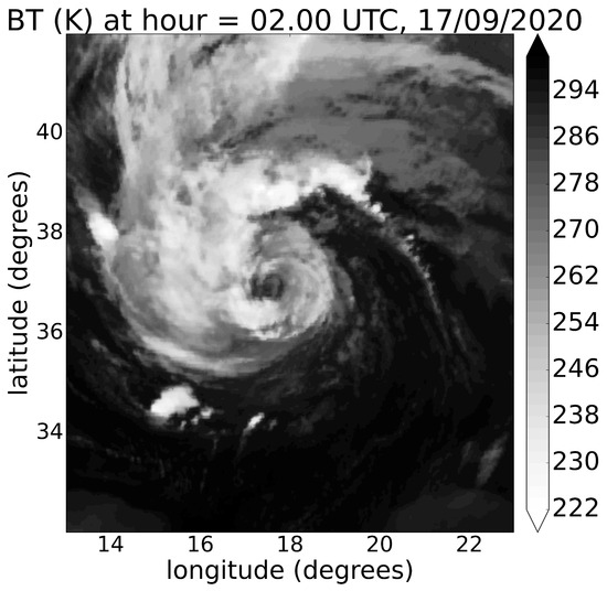
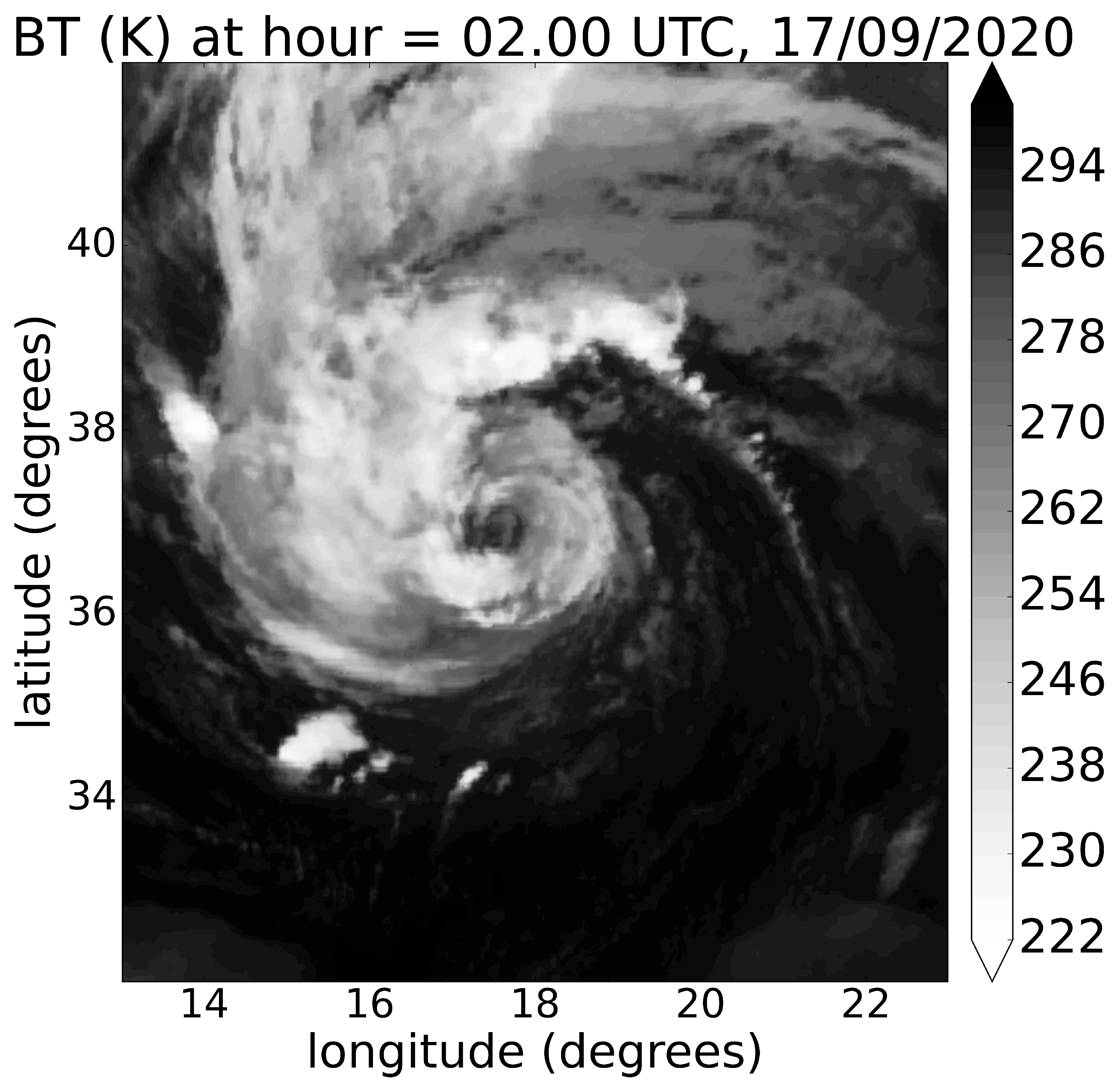
Ianos represents the most intense cyclone recorded in the Mediterranean basin in recent years [26]. The system originated within a cyclogenetic zone associated with strong convective activity near the Gulf of Sidra, early in September 2020, on the 15th day. In the following hours, it underwent rapid intensification, reaching markedly low central pressure and exhibiting a strong potential for acquiring tropical characteristics, sustained by elevated sea-surface temperatures. From late in the day on the 16th to the early hours of the 17th, Ianos continued to strengthen over the Ionian Sea, as illustrated in Figure 1 (image acquired by the Spinning Enhanced Visible Infrared Imager—SEVIRI database from Meteosat Second Generation—11 geostationary satellite), developing a clear eye and the defining features of a Medicane. Peak intensity was reached near the Greek coast during the first three hours of the 18th day, when the system attained an intensity equivalent to a Category-2 hurricane on the Saffir–Simpson scale. In the subsequent hours, it expanded considerably. Over the following two days, after making landfall in Greece, Ianos gradually weakened and ultimately dissipated near the eastern Libyan coastline.
Figure 1.
The intensification of the Ianos TLC acquired from a SEVIRI snapshot of 17th September, 02.00 h UTC.
The next section presents an overview of the methodologies for these two different macro-analyses, with the detailed steps of the spatio-temporal decomposition and the remote sensing techniques. Afterwards, two separate sections are shown for the associated results. Discussions and conclusions about this work are reported at the end.
2. Materials and Methods
The working line follows the analyses in two different approaches, exploited in a combination of remote sensing characterisation and spatio-temporal decomposition, hereinafter explained in the two separate subsections, for GEO and LEO datasets, respectively.
2.1. GEO Database: Ianos Spatio-Temporal Dynamics
Looking at the GEO satellite capabilities, a spatio-temporal analysis is conducted using data from SEVIRI onboard (MSG-11) mission, in the IR10.8 and WV6.2 spectral channels, considering the High-Rate and the Rapid Scan High-Rate acquisition services. These provide satellite products with a pixel size of 3 km (at the nadir) in spatial resolution and 15 min and 5 min time steps of temporal resolution, respectively, for the same total period of 96 h (4 days) of the Ianos lifecycle. The datasets thus include 384 and 1152 images from the two different services, respectively, exploring the above-cited scalar fields.
The specifics of GEO data acquisitions of Ianos life days evolution are reported in Table 1.
Table 1.
The characteristics of the exploited GEO products for Ianos evolution; all of them are acquired from the IR10.8 (TIR) spectral channel. Subscripts (1) and (2) represent High-Rate and Rapid Scan High-Rate acquisition services, respectively.
For these GEO datasets, we followed the Ianos dynamics using the same approach that was recently applied for TC analyses [24,25,27].
In the context of turbulent-flow dynamics, typically analysed through Fourier-based decomposition methods [28,29,30], the evolution of a TLC system such as Ianos can be investigated by exploiting the properties of the proper orthogonal decomposition (POD) technique [31]. POD enables the characterisation of how energy is distributed and evolves across multiple spatial and temporal scales, isolating persistent flow structures associated with the specific event. Compared with classical expansions (e.g., Fourier or Wavelet), POD is often preferred because it preserves the behaviour at the boundaries of the spatial domain, providing a rigorous mathematical framework for describing turbulent fields that exhibit coupled spatial and temporal organisation [32]. In particular, in these systems, the dominant energetic features are spatially localised and transient, rather than periodic. In such conditions, classical Fourier or wavelet decompositions—although effective for homogeneous turbulence—are not optimal for isolating the most energetic flow structures, which do not generally correspond to plane waves. For this reason, the POD is used to provide a complementary, energy-optimal framework that extracts data-adaptive modes directly from the observed field, allowing the identification of persistent coherent structures while preserving boundary effects and spatial localisation [24,25,27].
In its general formulation, the POD methodology begins with a set of snapshots of a scalar or vector field, , defined on a generic point, , where is the spatial domain at certain discrete times, . The focus of the application is its decomposition into an optimal basis for this system, described through a denumerable set of basis functions, , depending only on the spatial coordinates and time-dependent modal coefficients, :
This formulation separates spatial and temporal dynamics, allowing them to be analysed independently.
The functions can be written as the solutions of the following eigenvalue problem (Fredholm integral equation):
The average is computed over the ensemble of field snapshots at time . Accordingly, the optimal basis is defined by the eigenfunctions of Equation (2), whose kernel is associated with the time-averaged autocorrelation function
The eigenfunctions are mutually orthogonal, while the eigenvalues are real and positive, and they represent the time-averaged energy content of the j-th POD mode. This decomposition exhibits several useful mathematical properties that help verify the correctness of both eigenfunctions and coefficients. For example, the expansion coefficients must satisfy the uncorrelatedness condition (), and the sum of all eigenvalues must equal the total turbulent kinetic energy of the flow:
where E denotes the turbulent kinetic energy averaged in time. Since it can be directly computed from the original dataset, this relation provides a straightforward check on the calculation of the eigenvalues. Moreover, because the diagonal part of the correlation tensor, , corresponds to twice the local kinetic energy, each eigenfunction maximises the residual energy of the flow; the associated POD modes, therefore, identify the most energetic and coherent structures of the turbulent field.
All the previous properties of the POD coefficients and eigenfunctions (the orthogonality of the basis functions, the real and definite positiveness of the eigenvalues, the uncorrelatedness of the expansion coefficients and the equality of the average energy with the sum of all eigenvalues) have been extensively tested. Moreover, to ensure the convergence of the method, we checked that the product of the coefficients of the expansion, times the eigenfunctions, correctly reproduces the original field in both time and space, according to Equation (1).
Given the optimality condition, only a subset of eigenvalues contributes meaningfully to the analysis, following a commonly adopted selection criterion that retains only those eigenvalues carrying more than of the average energy. The following analysis, therefore, focuses on the most energetic modes. Furthermore, for a positive–definite dataset, the temporal mean is subtracted from each snapshot so that the decomposition captures only the fluctuating component, which is typically more informative for turbulence characterisation.
The solutions of Equation (2) consist of an infinite set of real, positive eigenvalues, , and an equivalent set of real eigenfunctions, , mutually orthogonal in space. These solutions describe the spatial behaviour of the system dynamics, owing to their orthonormal properties [33,34,35]. The energetic cascade that comes from the spectra can be associated with the effects of the stratification and the rotation of the anisotropic fluids [36] despite the atmospheric mesoscale of a cyclonic event showing specific features. In the context of these extreme events, POD modes highlight characteristic dynamical scales, enabling the reconstruction of the examined field using partial sums over selected spatio-temporal intervals. The contribution of a prescribed scale range () is expressed as
The POD technique is employed to analyse the energy distribution and evolution at different spatio-temporal scales during the entire lifecycle of Ianos, as well as within its distinct phases. The methodology involves the spectral decomposition of two scalar fields: cloud-top temperature, , and atmospheric pressure, P. Both fields are analysed on fixed 350 × 350 pixel domains centred on the cyclone, without zero-padding or the artificial extension of the spatial grid. For each variable, the temporal mean over the selected analysis window was removed so that the POD modes describe energy associated with dynamical fluctuations. The SEVIRI radiometer provides measurements of the brightness temperature, , dependent on the sensor’s central wavelengths ( for TIR and for WV). Although represents the radiance recorded at the instrument, it is not a direct temperature value. Following the empirical procedure used in [24,25] for tropical cyclone analyses, the cloud-top altitude, H, and the associated temperature field, are derived for the Ianos clouds. Their estimation relies on two linear relations (Equation (4)), characterised by constant lapse-rate parameters representing the decrease in the air temperature (9.84 K per 1000 m) and the dew-point temperature (1.82 K per 1000 m) with altitude. These relations allow for the retrieval of H and from the daily averaged near-surface air temperature (). The computation assumes that, under sufficiently unstable conditions, the satellite-measured brightness temperature approximates the dew point, , at the condensation level. Thus, the system
is solved with the constraint , yielding the expressions for H and reported in Equation (5):
We highlight that the retrieval of and H relies on simplified thermodynamic assumptions, including constant lapse rates. In strongly convective environments, such as during the TLC mature phase, these assumptions may introduce systematic biases due to variations in moist–adiabatic lapse rates, cloud microphysical properties, and optical thickness. Accordingly, the retrieved quantities are interpreted here as effective thermodynamic proxies, rather than exact atmospheric state variables. The subsequent analyses focus on spatial and temporal variability and on the organisation of fluctuations, rather than on the absolute magnitude of the retrieved fields. Subsequently, pressure, P, is computed via the exponential law (Equation (6)), which incorporates the scale height estimated from temperature variations between 8 km (near-surface layers) and 6 km (upper, colder layers) [37,38].
The law explains the evolution of the pressure with from = 1013.25 hPa, corresponding to the surface pressure under standard conditions, over the different layers of the atmosphere, depending on H, directly obtained from the previous system. Remarkably, this is not a direct MSLP estimate, but specifically, the retrieval provides an effective warm-core pressure proxy linked to the vertical extension of the cloud system because of the strongly convective and non-isothermal conditions.
The results of the POD analysis applied to these parameters include the Ianos dynamics over the whole period (sub-an. GEOa) and a spatio-temporal investigation during three crucial phases of the Ianos evolution (formation, peak intensity, and final weakening-sub-an. GEOb).
Furthermore, a characterisation of the deep convection associated with the cyclonic clouds is performed following the remote sensing algorithm that provides the deep convective cloud pixels (DCCPs) from the spectral channels of SEVIRI. In particular, since there is no universal threshold directly from the TIR channels for the detection of deep convection, the criterion of adopting < 208/210 K as a DCCP indicator for the clouds [22,39] is used as the first test in the selected images of Ianos’s evolution The method is then optimised by considering the brightness temperature difference (BTD) between spectral channels at 6.7 μm (water vapour—WV—channel) and the ones at 10.8 μm (TIR) in order to detect the presence of thick clouds (Equation (7)) [40].
From this method, the small values (BTD ≤ 0 K) coincide with high convective clouds (sometimes reaching the troposphere), while positive ones (BTD > 10 K) are associated with low stratiform clouds. Some recent studies show a more precise description of the threshold values, based on the convective storm [41] and tropical cyclone convection [42], where the DCCP mask is much more significant in the detection of the same clouds. We selected the criterion used in [43], in which the deep convective mask is characterised by the combination of three conditions: (1) < 240 K values; (2) −5 K < BTD < 15 K values; (3) 3 K < < 8 K values, where corresponds to the local standard deviation on values. It is important to note that the adopted DCCP criteria are not locally calibrated for the specific thermodynamic conditions of a TLC, but they can be interpreted as a qualitative indicator of deep convective cloud organisation, rather than as a quantitative measure of convective intensity or precipitation. For each pixel in all the Ianos images, when the mask satisfies the conditions, DCCP = 1; otherwise, DCCP = 0. In the results, there is a subsection (sub-an. GEOc) that includes the examples of this application.
Finally, we highlight a comparison between the POD spectra obtained for Ianos on its day of maximum intensity and those derived for TCs Faraji and Freddy, to qualitatively identify potential analogies and differences between the two types of cyclones (sub-an. GEOd).
2.2. LEO Database: The Daily Trends of Some Key Parameters
In this section, we analyse the images acquired by three LEO satellites: Sentinel-3A/B, equipped with the Sea and Land Surface Temperature Radiometer (SLSTR), and Suomi NPP, carrying the Visible/Infrared Imager Radiometer Suite (VIIRS). These sensors enable global coverage at a low-to-moderate spatial resolution (nadir pixel sizes of 0.1 and 10 km) and a moderate temporal resolution of 1–2 images per day, thus capturing the daily evolution of Ianos as an extension of the analyses presented in [21].
The satellite observations are processed to derive physical quantities, such as cloud-top altitudes and temperatures, vertical temperature gradients, and atmospheric pressure fields, following the methodology established for tropical cyclone studies [24]. The altitude and temperature values are computed using standard atmospheric lapse-rate conditions for both air temperature and dew point, while the sea surface temperature is incorporated into the evaluation of atmospheric instability through the vertical temperature gradient. The pressure field is likewise obtained under the same standard assumptions. In this framework, air and sea temperature values are obtained from the BOLAM forecasting model [44,45] and the ERA5 reanalysis dataset.
The atmospheric instability conditions are evaluated using the TLC-derived values of H and , through the vertical temperature gradient , which expresses the relation between temperature variation within the cyclone layers and altitude (Equation (8)):
where denotes the model-derived daily averaged sea surface temperature. Since exceeds in all scenes except those directly associated with the sea surface, this formulation provides a local signature of the thermal stratification relevant to cloud development. Interpreted in this framework, the resulting values describe how instability evolves during the TLC’s lifecycle, especially when compared with canonical atmospheric thresholds that classify the degree of instability:
- (1)
- : absolute atmospheric instability, corresponding to the dry adiabatic lapse-rate limit;
- (2)
- : conditional atmospheric instability, defined by the moisture-to-dryness ranges of vertical gradients.
Following our interpretation, the resulting vertical temperature gradients could, therefore, be considered indicators of strongly unstable thermodynamic conditions. The full dataset of Ianos’s daily evolution, from the two different sensors, is presented in Table 2.
Table 2.
Spaceborne imagery acquired from the two sensors for Ianos’s daily evolution. Asterisk marks indicate satellite sensing at nighttime.
With these products, we perform the observation of the atmospheric daily instability of Ianos, particularly fixing the same geographic area for the VIIRS images (sub-an. LEOa). The results are also provided for the assessment of the pressure trends of Ianos’s behaviour in all the days of its evolution, comparing the values of the pressure measured in the warm core with mean sea level pressure (MSLP) from the BOLAM and ERA5 datasets (sub-an. LEOb).
3. Results
3.1. POD Results on the Whole Periods of the Ianos TLC’s Evolution
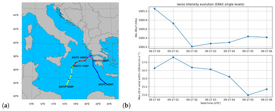
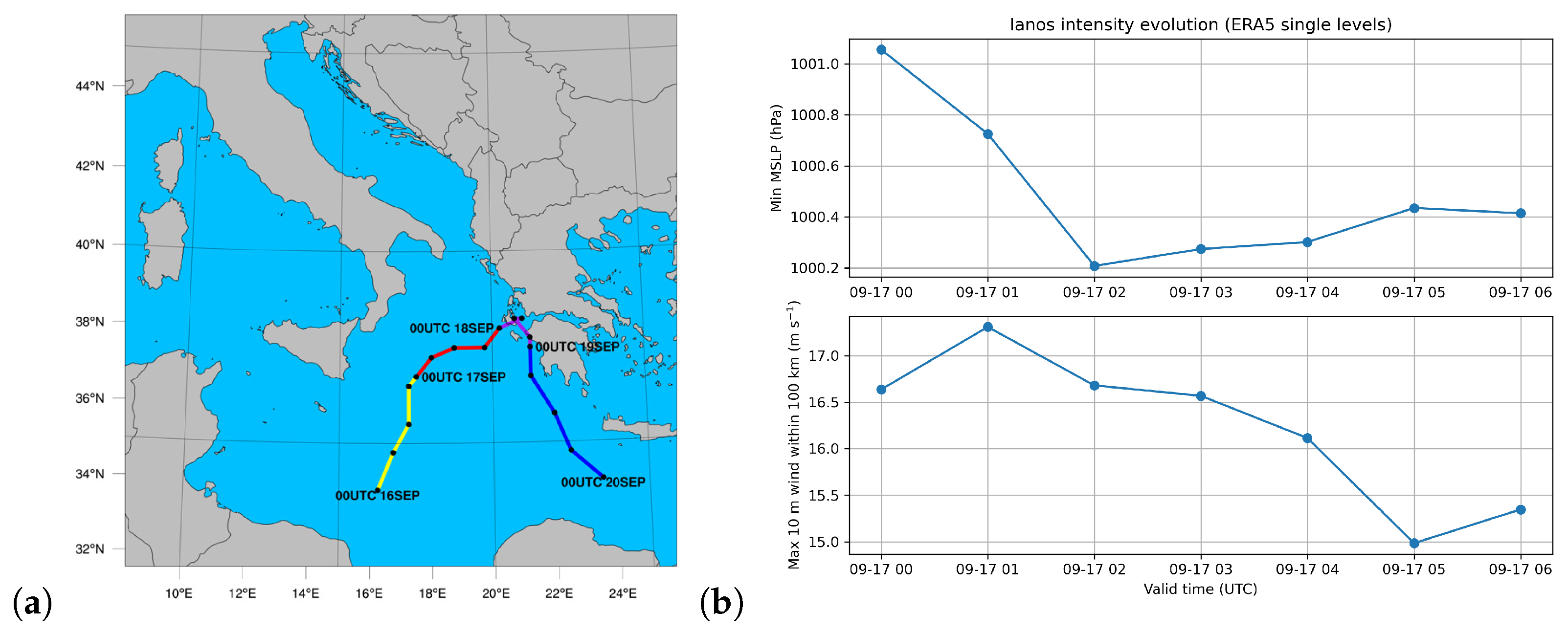
The initial step involves the POD application to the entire SEVIRI database, spanning 4 days of Ianos’s significant development, including the path between 15th September, 00.00 UTC, and 19th, 00.00 UTC, covering all the Ionian Sea. The POD analysis is performed on both the 384 and 1152 products of the two different acquisition services corresponding to this period. The path of Ianos is shown in Figure 2a [16], from which the spatial grid, used for our analyses, is fixed and identified by considering the domain between 14° E ad 24° E of longitude and 30° N and 40° N of latitude for all the SEVIRI snapshots. In this way, it is possible to look at the Ianos displacement in this geographical area during its temporal evolution. Additionally, the latter is shown in Figure 2b, quantifying the minimum sea-level pressure (upper plot) and the maximum near-core 10 m wind speed (lower plot) derived from ERA5 single-level fields. They are considered to contextualise what comes next in the POD-based multiscale analysis and the cloud-top structural changes.
Figure 2.
Panel (a): Representationof the displacement of Ianos in the days of its evolution during its Medicane phase. The Bullet points identify the centre of the cyclone [16]. The colours in the trajectory identify different intensity stages during the evolution of the TLC: yellow corresponds to the passage to the Medicane state, red is the maximum intensity, and blue represents the first weakening. Panel (b): the time evolution of Ianos’s intensity derived from ERA5 single-level fields, with the minimum sea-level pressure (upper plot) and the maximum 10 m wind speed within a 100 km radius from the centre (lower plot).
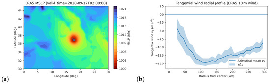
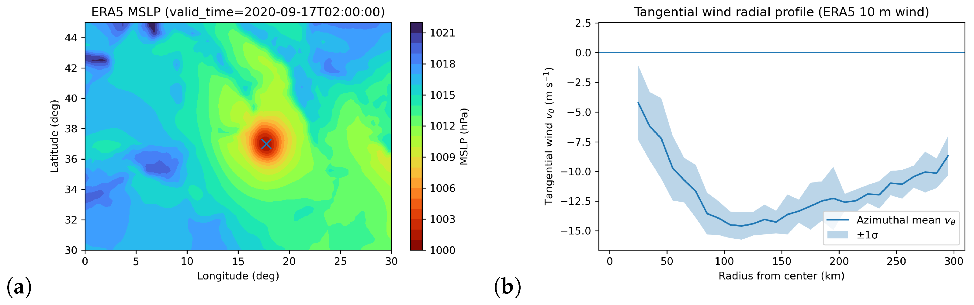
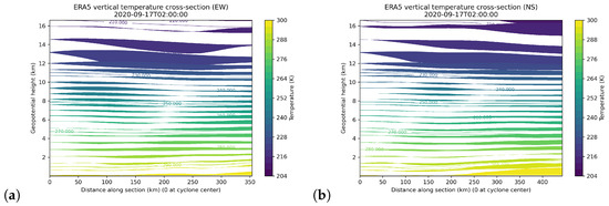
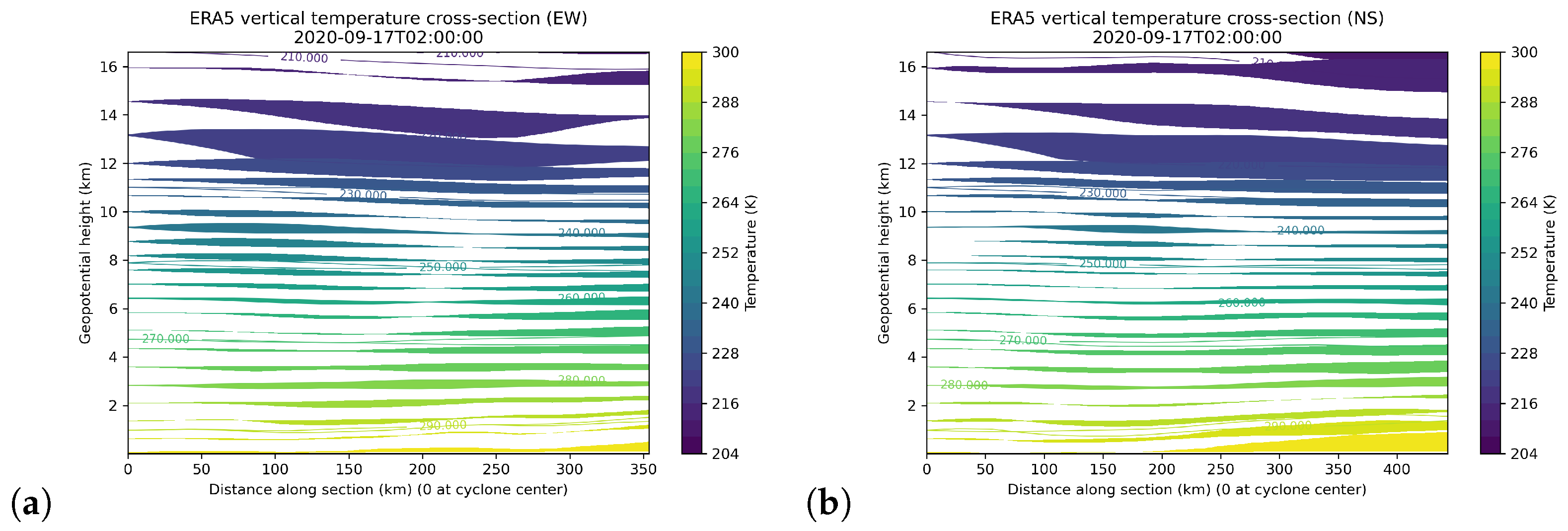
The structural characteristics of the TLC at the intensity peak provide a clear physical context; in Figure 3, the near-surface core structure is shown from ERA5 database. In particular, the peak is characterised by a central low-pressure region in the MSLP map (panel a), and a radial maximum of the tangential wind speed (panel b) is consistent with an eyewall-like feature. The Ianos vertical thermal structure at the peak intensity is further examined using ERA5 pressure-level fields, as shown in Figure 4, which documents the presence of a vertically coherent warm-core structure across the troposphere in the east-to-west direction (panel a) and the north-to-south direction (panel b).
Figure 3.
Near-surface structural characteristics of Ianos at peak intensity (2020-09-17 02.00 UTC) derived from ERA5 single-level fields. Panel (a): spatial distribution of mean sea-level pressure, with the diagnosed cyclone centre marked. Panel (b): azimuthally averaged tangential wind speed as a function of radial distance from the cyclone centre, highlighting a weak-wind core region and a maximum at finite radius.
Figure 4.
Vertical thermal structure of Ianos at peak intensity derived from ERA5 pressure-level fields. The cross-section of temperature in geopotential height coordinates is along a section passing through the diagnosed cyclone centre, highlighting a vertically coherent warm-core structure extending in the east-to-west direction (panel (a)) and the north-to-south direction (panel (b)).
The first stage of the analysis examines the field. A 2D FFT is applied to each snapshot—after the temporal average value is subtracted—to obtain shell-integrated spectra. Through this transformation, each image is mapped into wavevector space () and partitioned into concentric circular shells. The energy contribution associated with each shell is then computed by summing the energies of all Fourier modes contained within it. When averaged over all time steps, this procedure reveals a strong correspondence between the POD spectrum and the extracted eigenfunctions, enabling a direct assessment of the spatial energy distribution. In the shell-integrated spectra, the energy trend is represented on a bi-logarithmic scale and reflects the spatial component of the dynamics. A complementary representation is given by the temporal coefficient spectrum, which describes the average energy distribution of the expansion across POD modes as a function of characteristic frequencies. Both spatial and temporal spectra exhibit power-law behaviour, with distinct slopes across three scale intervals. The breakpoints separating these regions are identified following the procedure outlined in [24,27], where linear fits are applied to the bi-logarithmic spectra. Specifically, spectral slopes and transition scales are determined through a piecewise linear fit, in which adjacent spectral zones are fitted simultaneously under continuity constraints, and the breakpoint location is treated as a free parameter. This approach allows the objective identification of scale-dependent spectral regimes, avoiding arbitrary segmentation. These breakpoint values define the spectral boundaries for the partial POD reconstructions used to recover temperature fields at different characteristic scales.
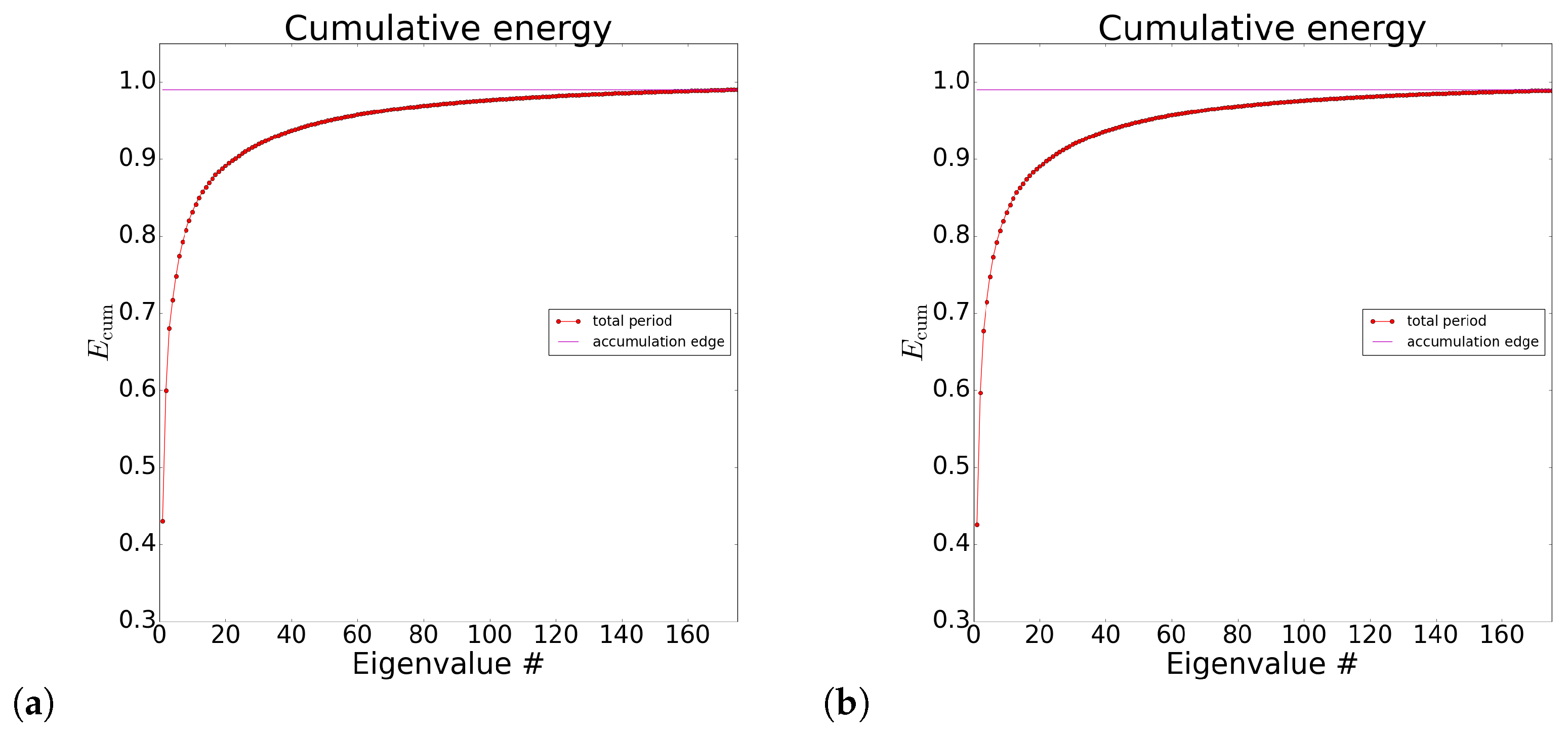
The POD decomposition yields a set of spatial eigenfunctions, , and associated temporal coefficients, , together with a sequence of eigenvalues, (with or 1152, depending on the configuration), which quantify the time-averaged energy contained in each mode and are sorted in descending order. The robustness of the POD modes with respect to the number of snapshots was assessed by comparing analyses with different sample sizes, confirming the convergence of both the leading modes and the associated energy spectra. In particular, the cumulative energy of the modes is shown in Figure 5 (red dots), which converges to the selected threshold corresponding to the 99% of the energy (blue lines), for the two configurations. As the temperature is a positive-definite quantity, this comparison leads to take into account the fluctuation values (subtracting the average temperature value), putting the main focus on capturing the spatial and temporal evolution of the turbulent structures.
Figure 5.
Cumulative energy from the number of the POD eigenvalues, attaining the threshold of the 99% of the average energy of the Ianos temperature field, in the 15 min time step case (panel (a)) and in the 5 min time step case (panel (b)).
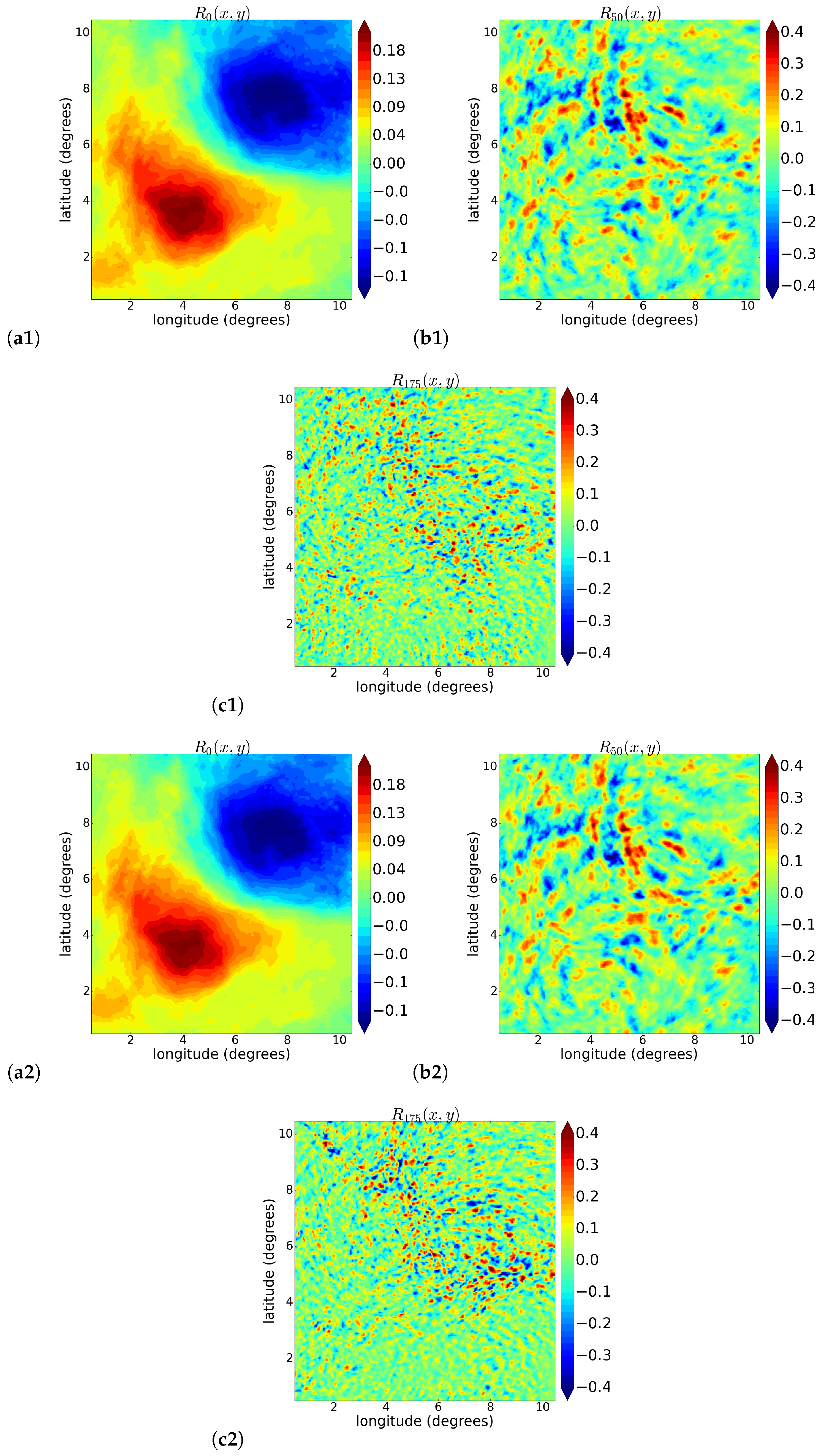
As in the previous analyses, the selection of the most meaningful modes is performed by retaining only those eigenvalues whose cumulative sum accounts for of the average energy, included in the most energetic eigenvalues for both cases. The POD is applied on the field by considering the total periods, and the very first result concerns the eigenfunctions, reported in Figure 6. More precisely, in the panels (a1), (b1) and (c1), examples of three eigenfunctions related to the High-Rate service acquisition (with time step of 15 min) are shown, while panels (a2), (b2) and (c2) refers to the same examples but for the Rapid Scan High-Rate case. Following the same approach used for the Faraji and Freddy TCs, it is possible to relate the POD eigenfunctions with large, intermediate and small scales, respectively associated with the orders . This association, as explained in [24,25,27], is not imposed a priori and does not imply a one-to-one correspondence between a POD index and a specific physical length scale. Instead, characteristic scales are inferred a posteriori from the spectral content of the POD eigenfunctions. For each mode, the shell-integrated Fourier spectrum exhibits a dominant peak in wavevector space, whose position provides an estimate of the characteristic length scale of that eigenfunction. Due to the non-periodic nature of the data, discretisation effects, and the intrinsic anisotropy of the structures along the longitude and latitude directions, these spectral peaks are not delta-like but spread over a finite range of wavevectors. Nevertheless, we observed the same trend obtained for the TCs’ analysis: as the POD mode order increases, the dominant spectral peak shifts progressively toward higher wavevectors, indicating smaller characteristic spatial scales. This monotonic shift provides a physically consistent basis for grouping POD modes into large-, intermediate-, and small-scale ranges. From the plots, it seems that, while at large scales there is not a significant difference between the two cases, at the smaller scales, we can see more structures surviving in the oscillations related to the 5 min evolution steps.
Figure 6.
The POD eigenfunctions contour plots of the Ianos evolution, as a function of longitude and latitude, for the modes , and , corresponding to large, intermediate and small scales: panels (a1–c1) refer to the 15 min time step case, while (a2–c2) refer to the 5 min time step case.
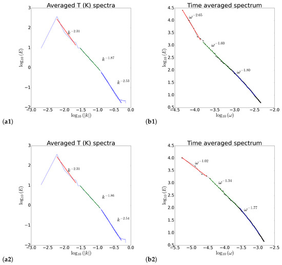
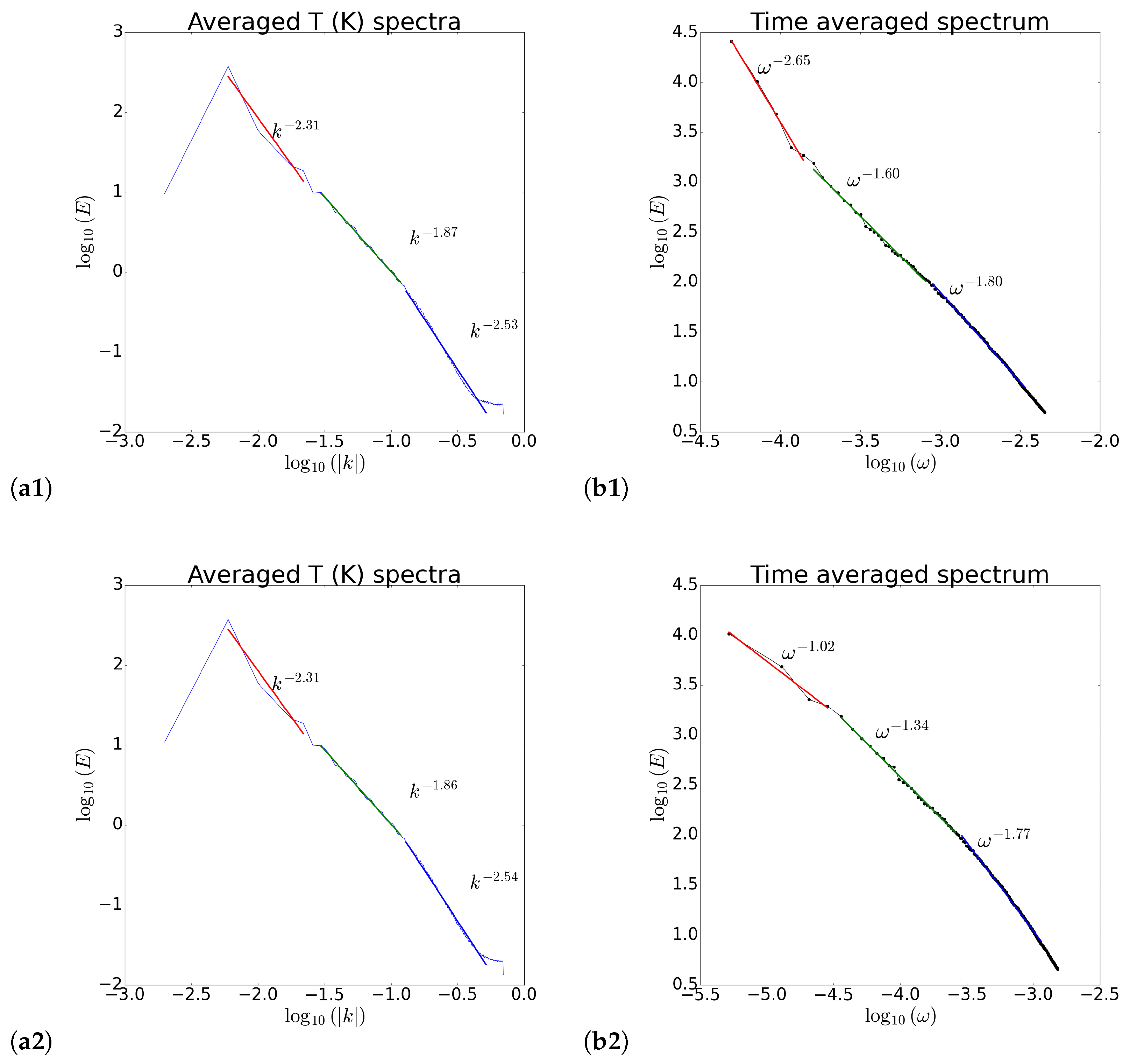
In Figure 7, the shell-integrated k spectra (panels a1, a2) and the energy-frequency spectra (panels b1, b2) are reported for both cases. Strong similarities in all the scale ranges are found in the spatial component spectra for the two cases. However, the energy spectra as a function of the frequencies show different trends, with more significant differences at the largest scales, related to the larger number of time steps available for the POD expansion in the 5 min case. The intermediate and small scales’ intervals show the decrease in energy with the power-law characteristic trend.
Figure 7.
Panels (a1,a2): the shell-integrated spectra of the spatial component of the total database of the Ianos dynamics, averaged over all sensing times, for 15 min and 5 min time steps, respectively. Panels (b1,b2): the time-averaged spectrum of the POD temporal component of the Ianos field, for 15 min and 5 min time steps, respectively.
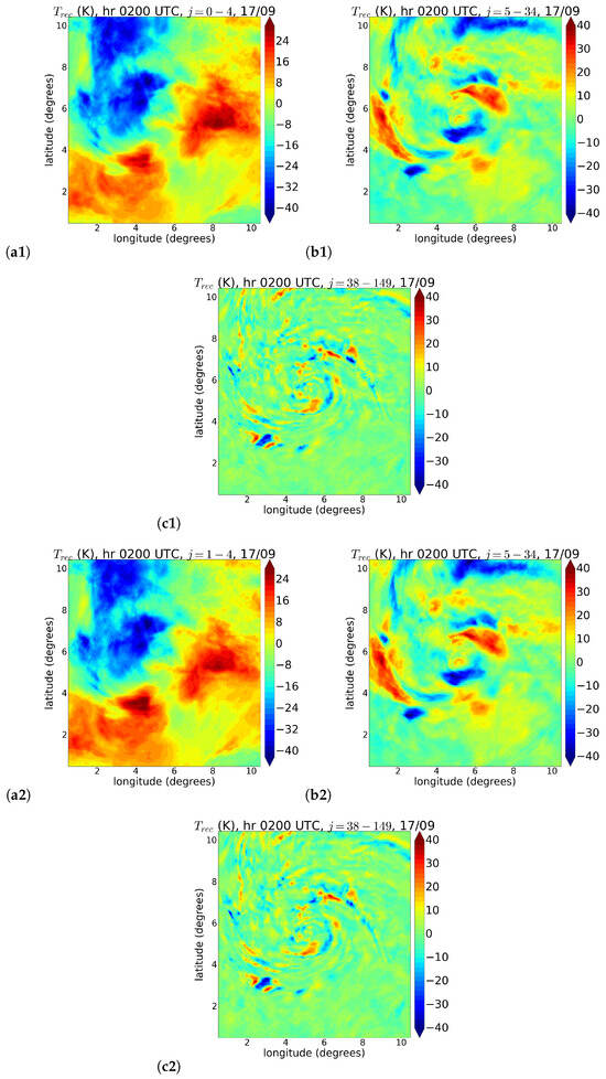
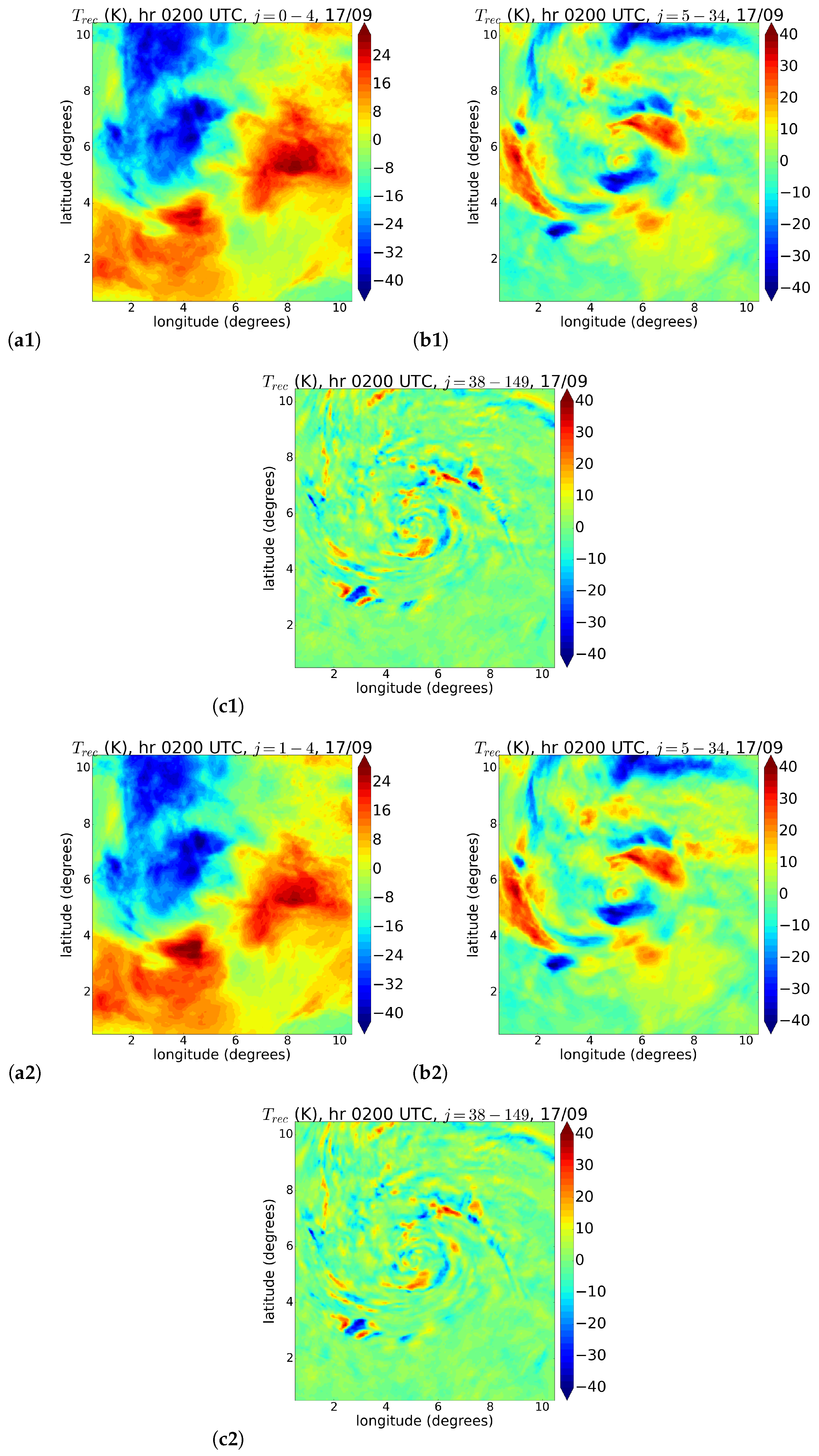
The spectral analysis characterises scale-dependent organisation but does not directly quantify nonlinear inter-scale energy transfers (e.g., spectral fluxes), which would require more dedicated diagnostics. Nevertheless, the results obtained concerning the separation of the spectra into three ranges of scales lead to the performance of reconstructions of the field of Ianos in the three characteristic scale ranges. By computing the partial sums of the POD modes over defined scale ranges from to , the field is reconstructed in the different ranges for all the time steps of Ianos’s evolution. In Figure 8, we report the example of a reconstructed field of Ianos at the sensing time corresponding to 02.00 h UTC of September 17th ( for the 15 min case, for the 5 min case). The chosen times correspond to the moment of the maximum intensity of the event. Large-scale reconstructions are presented in the panels (a1) and (a2), intermediate-scale ones are shown in the panels (b1) and (b2), and small-scale ones are shown in panels (c1) and (c2), respectively. It can be seen that large-scale oscillations show a strong positive trend in the regions of south-to-east rotating air masses, becoming significantly negative from north to west. The filamentary and spotty structures at the smaller scales are visibly more pronounced in the region of the warm core. Both configurations are similar in the trends for all the characteristic scales.
Figure 8.
Panels (a1–c1): reconstructed field (K) of Ianos at the large, intermediate and small scales, for September 17th, 02.00 h UTC, in the 15 min case (maximum intensification peak). Panels (a2–c2): the same reconstructions for the same day and time, in the 5 min case. For all images, the average value is subtracted.
3.2. POD Application on Three Different Phases of the Ianos TLC Lifecycle
With the same focus on understanding the evolution of the Ianos TLC dynamics, a further analysis is performed, once again leveraging the POD technique, but looking at three different stages of the Ianos lifecycle by considering the same databases. The results on the field are provided for both the cases of 15 min and 5 min time steps, in the stages of: (1) the very first intensification of the perturbation into a tropical-like cyclone (corresponding to the first 24 h of the total period—15th September), (2) the peak of the maximum intensity of the already formed TLC (24 h of 17th September), (3) the stages of the first weakening of the TLC (last 24 h, corresponding to 18th September).
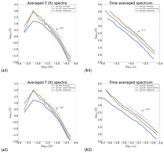
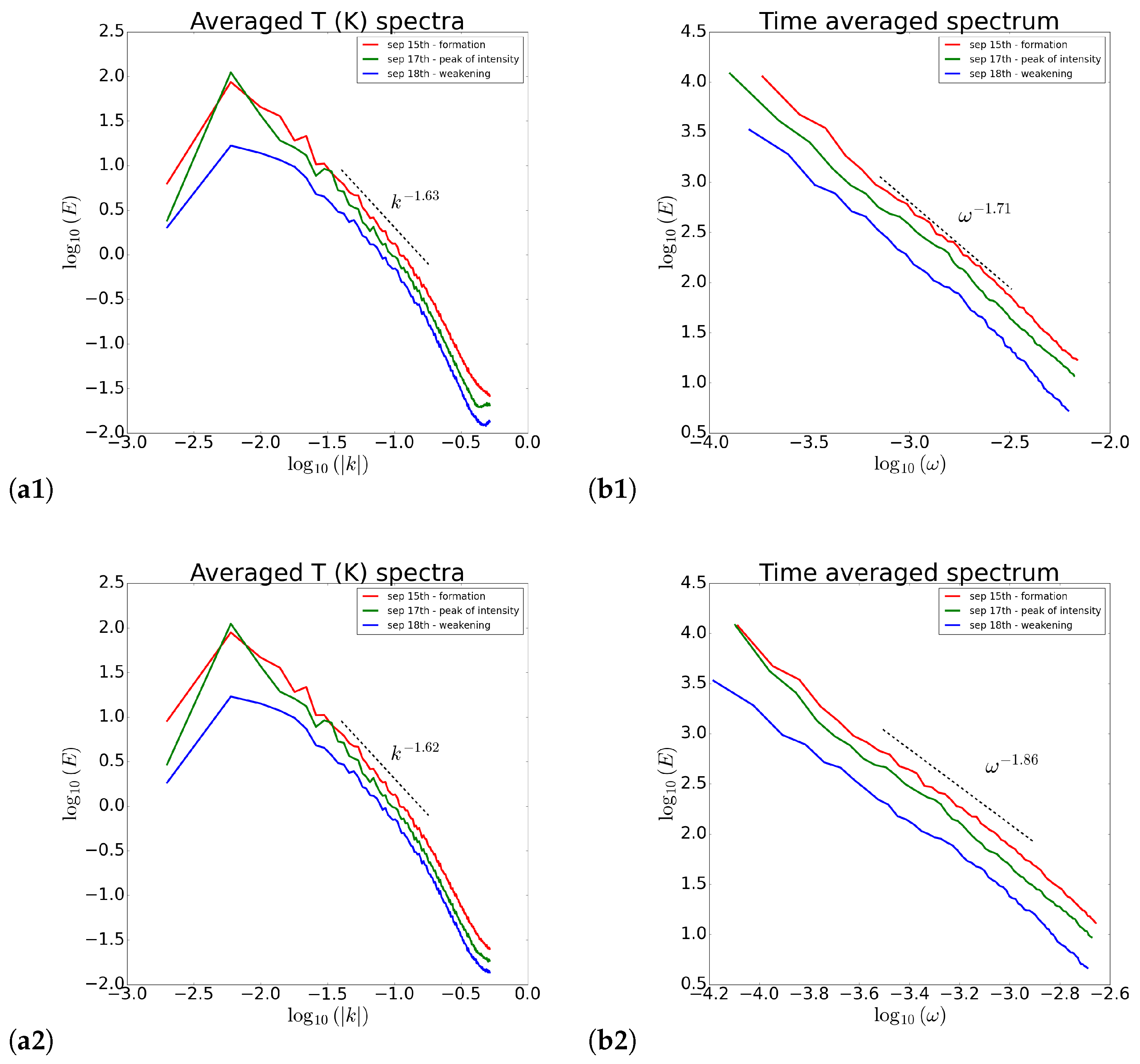
For these investigations, the results have to be considered in terms of a comparison between the different stages. Since it is well known that the comparison after the POD expansion can be possible only from looking at the energy distributions for spatial and temporal components separately, the results for the POD spectra obtained in the three cases are the only results reported. Thus, in Figure 9, shell-integrated spectra (panels a1, a2) and time-averaged spectra (panels b1, b2) for the three stages are shown, always considering the two different cases. The fitting power-law shown for all the cases is computed by considering an average value of the energy trend in the intermediate scale, characteristic of the transition of the energy distribution. From these comparisons, it is found that the spatial component has, in both configurations, the same characteristic trends, with almost identical spectral indices. However, the same strong similarity is not observable in the temporal component, taking into account the difference in the number of time steps. The intermediate scale preserves an approximated trend, especially in the spectra of the spatial component.
Figure 9.
Comparison between the energy spectra of the three stages of the Ianos lifecycle. Panels (a1,a2): shell-integrated spectra of the spatial component, averaged over all the sensing times, for 15 min and 5 min time steps respectively. Panels (b1,b2): time-averaged spectrum of for 15 min and 5 min cases, respectively.
3.3. Deep Convective Clouds Pixel (DCCP) Detection Inside Ianos
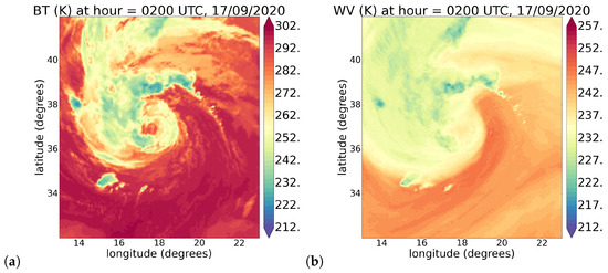
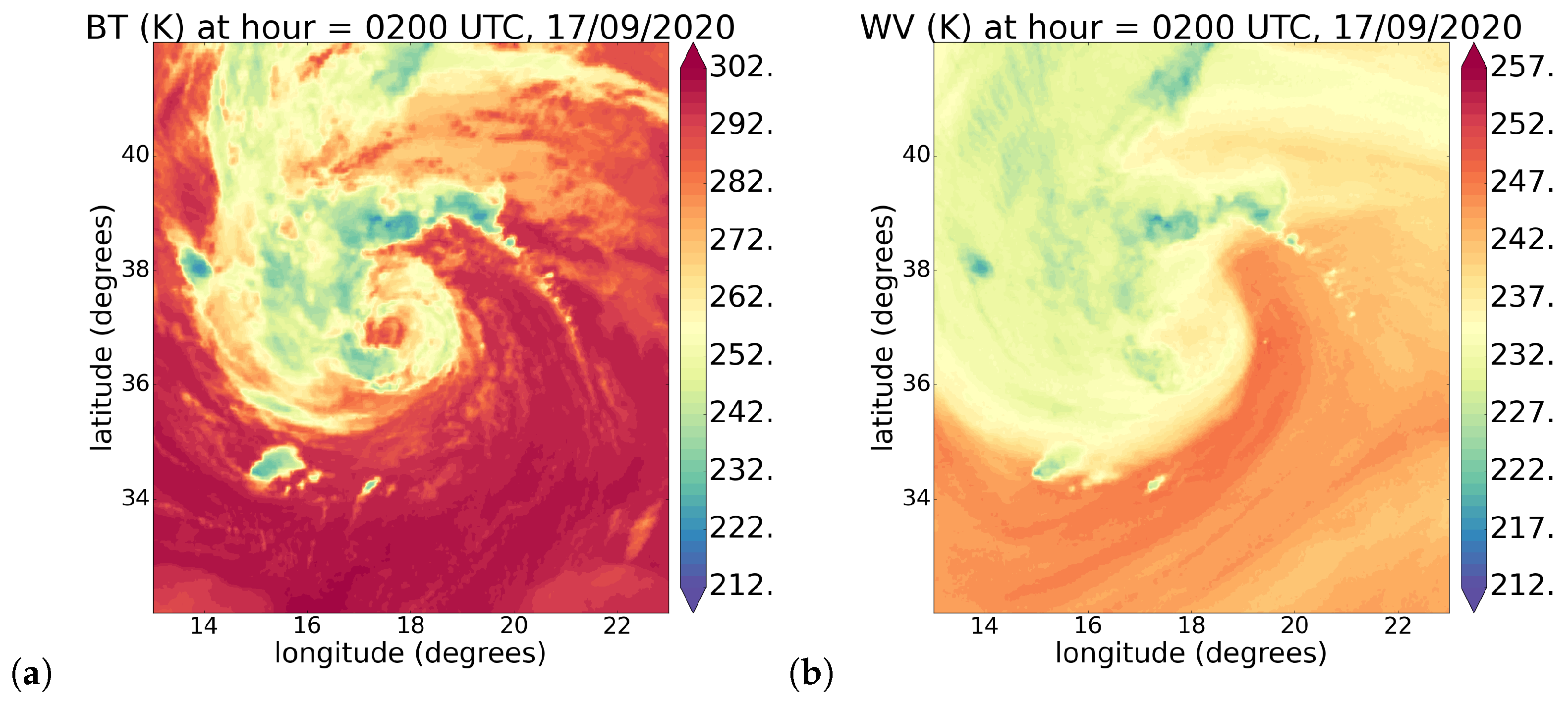
A qualitative assessment concerning the specifics of the cloud inside Ianos system is given with the SEVIRI products’ elaboration for detecting the pixels of deep convection. Since convection plays an important role in the intensification and tropicalisation of a Medicane, we perform its detection in the images by considering the criterion in which the focus is based on the field extracted from the SEVIRI TIR and WV spectral channels [43]. Ianos products for the two different channels are shown in Figure 10, representing the time of the Ianos intensity peak.
Figure 10.
values (K) of Ianos product of 17th September, 02.00 h UTC, for TIR 10.8 (a) and WV 6.2 (b) SEVIRI spectral channels.
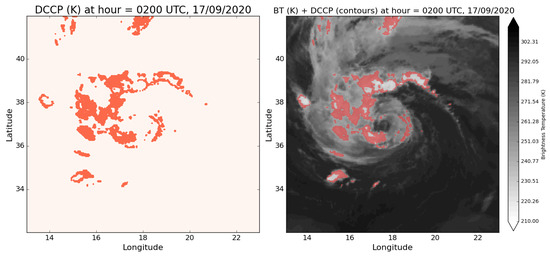
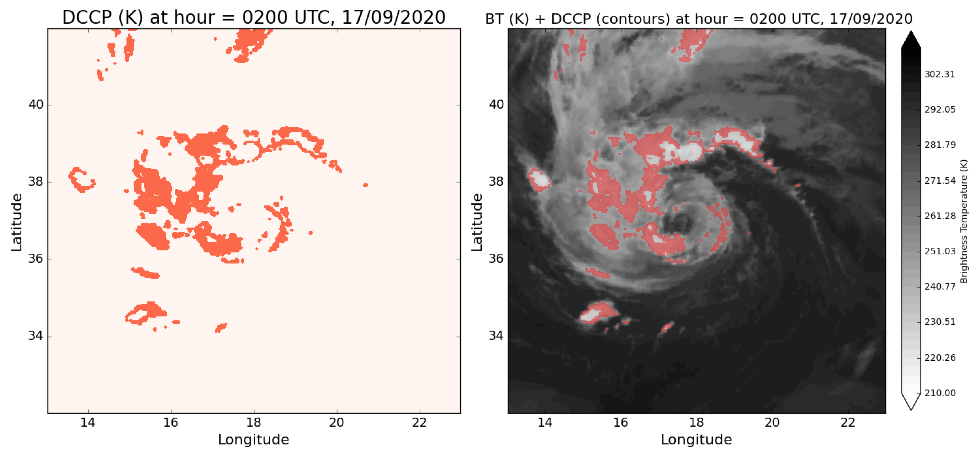
The algorithm of DCCP detection provides the application of the difference between the values of the two channels, expressed as BTD, taking into account the conditions on the very high clouds, their optical thickness and the texture based on the standard deviation of . A DCCP mask is computed for all the sensing times in order to assess the evolution of the deep convection with Ianos. An example of the mask is shown in Figure 11, where the red points correspond to the deep convective clouds only (left panel) and its overlay on the Ianos total system (TIR channel—right panel) in the time of the intensity peak.
Figure 11.
DCCP detection for Ianos product of 17th September, 02.00 h UTC: mask only in the (left panel), overlay of the mask on values in the (right panel).
The apparent discontinuities of the DCCP mask in the eyewall region are consistent with the presence of a warm-core structure, where cloud-top temperatures may locally increase and thin cirrus layers or intermittent overshooting tops can reduce the sensitivity of fixed infrared thresholds. Nevertheless, during the peak intensity of Ianos, it seems that the DCCP distribution revealed a compact, spiral-shaped convective core with very low brightness temperatures (<230 K), indicating a mature warm-core structure and confirming the occurrence of organised deep convection. This is a typical behaviour of fully developed tropicalisation.
3.4. Ianos POD Results Compared with Faraji and Freddy TCs: The Case Study of the Intensity Peak
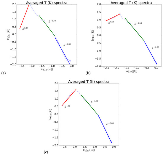
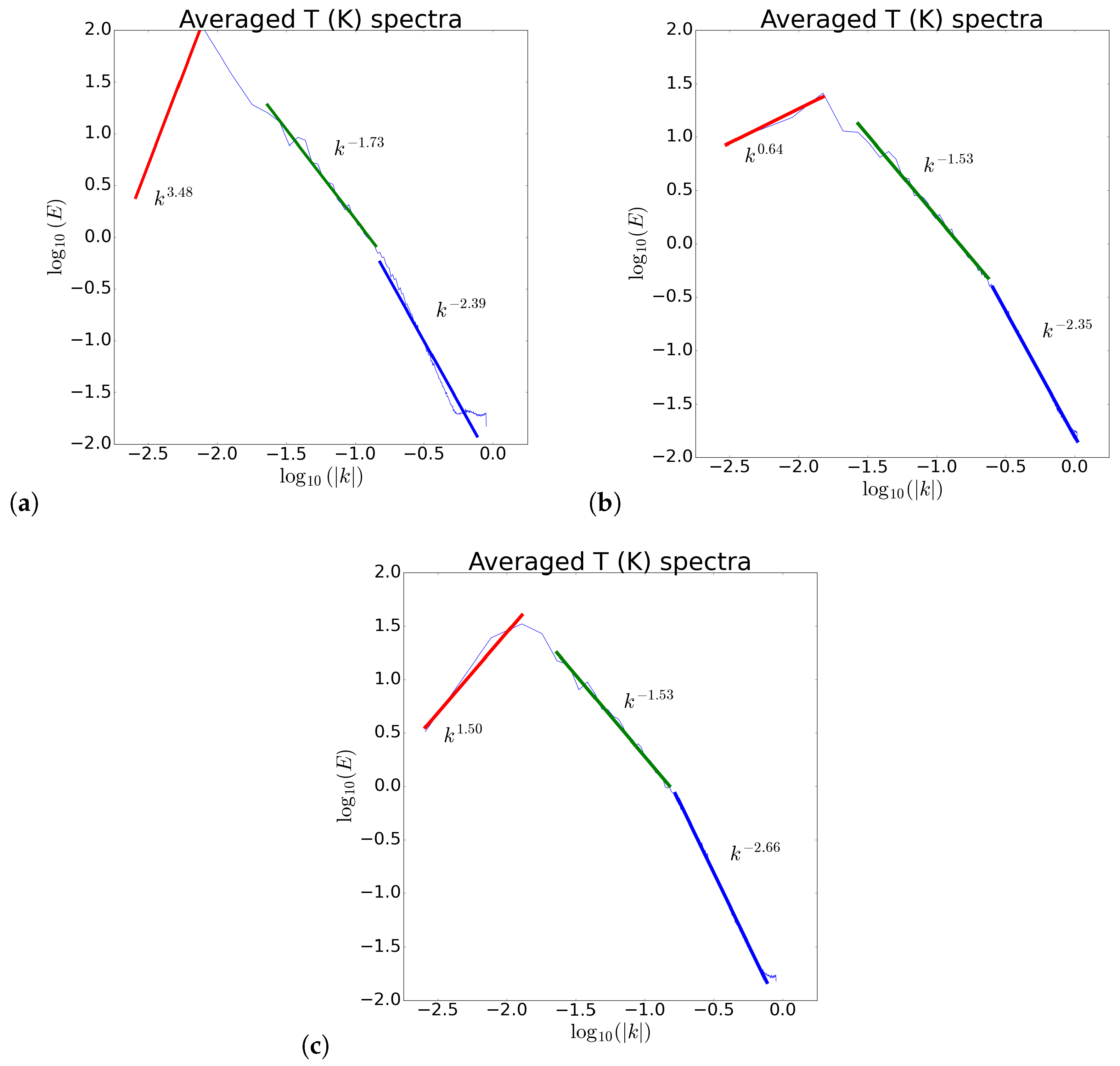
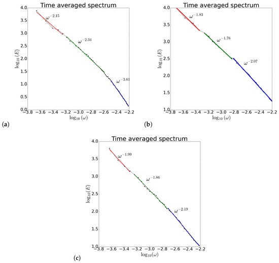
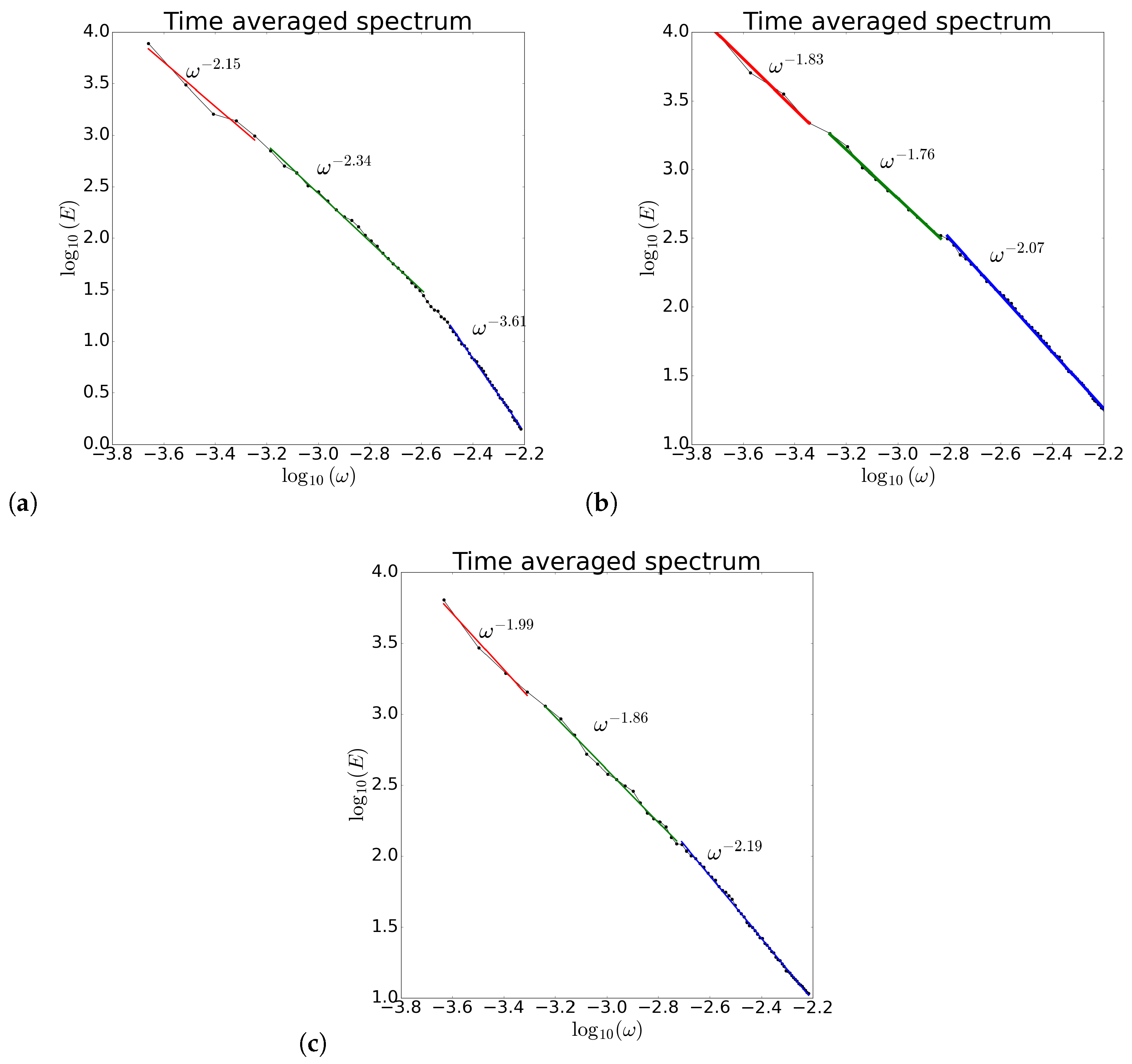
The last analysis of Ianos is focused on the attempt to compare the effects of its evolution, classified as a second-category tropical cyclone, with the ones obtained for events of tropical cyclones. For this reason, the POD expansion on the fields for the 24 h of the peak of intensity of Ianos, using the 15 min time steps, is considered for the comparison with the Faraji and Freddy results, in the same stage and with the same time step. Because of the total distinction of the events (they occurred in separate cyclonic seasons and different geographic areas), the comparison is exclusively performed among the energy spectra. We report the comparison between shell-integrated spectra of the three events in Figure 12, with the Ianos case in panel (a), Faraji in panel (b) and Freddy in panel (c). It can be seen that, while the spectral breakpoints and slopes are strongly similar in the TC cases, the Ianos case shows a different behaviour in all the scale ranges, with different values of the spectral slopes, despite the energy decreases with a very similar spectral shape. In Figure 13, the comparison between the time-average spectra of the three events is shown, and we can see that, in all the frequency ranges, the slopes are always very close to for the TC dynamics (panels b, c), while for Ianos (panel a), the spectrum is steeper. The decrease in energy in the temporal component seems to assume more typical behaviour in all the scale ranges, in the very first comparison between these different events, highlighting what is currently known about the similarities of their atmospheric evolution.
Figure 12.
Comparison between the shell-integrated spectra, associated with the spatial component of the dynamics of Ianos TLC (panel (a)), Faraji TC (panel (b)) and Freddy TC (panel (c)). The spectra refer to the 24 h of maximum intensity peak of the three events, with 15 min sensing times from the SEVIRI databases.
Figure 13.
Comparison between the time-averaged spectra of energy as functions of the frequencies, associated with the temporal component of the dynamics of Ianos TLC (panel (a)), Faraji TC (panel (b)) and Freddy TC (panel (c)). The spectra refer to the 24 h of maximum intensity peak of the three events, with 15 min sensing times.
Moreover, we added, in the Supplementary Material, animations of the temperature field, reconstructed according to Equation (3), corresponding to the large-(file RecMASC_IanosMaxInt.gif), intermediate-(file RecMESC_IanosMaxInt.gif) and small-scale ranges (file RecMISC_IanosMaxInt.gif), in the day of maximum intensification of Ianos, to better follow the temporal evolution of the roll-filament structures observed in the cyclone. Furthermore, we also added an animation (file Eigenfunctions_IanosMaxInt.gif) of the spatial representation of the eigenfunctions to show that increasing values of the spectral index correspond to smaller-scale structures.
3.5. Ianos Daily Evolution: Vertical Temperature Gradient and Instability
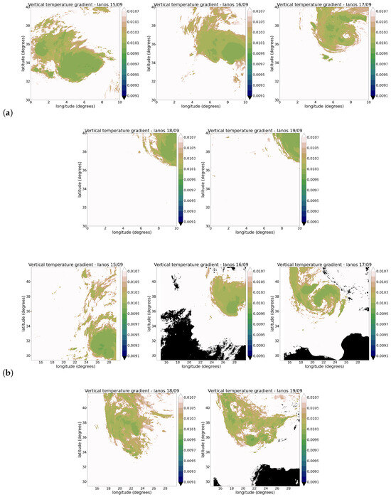
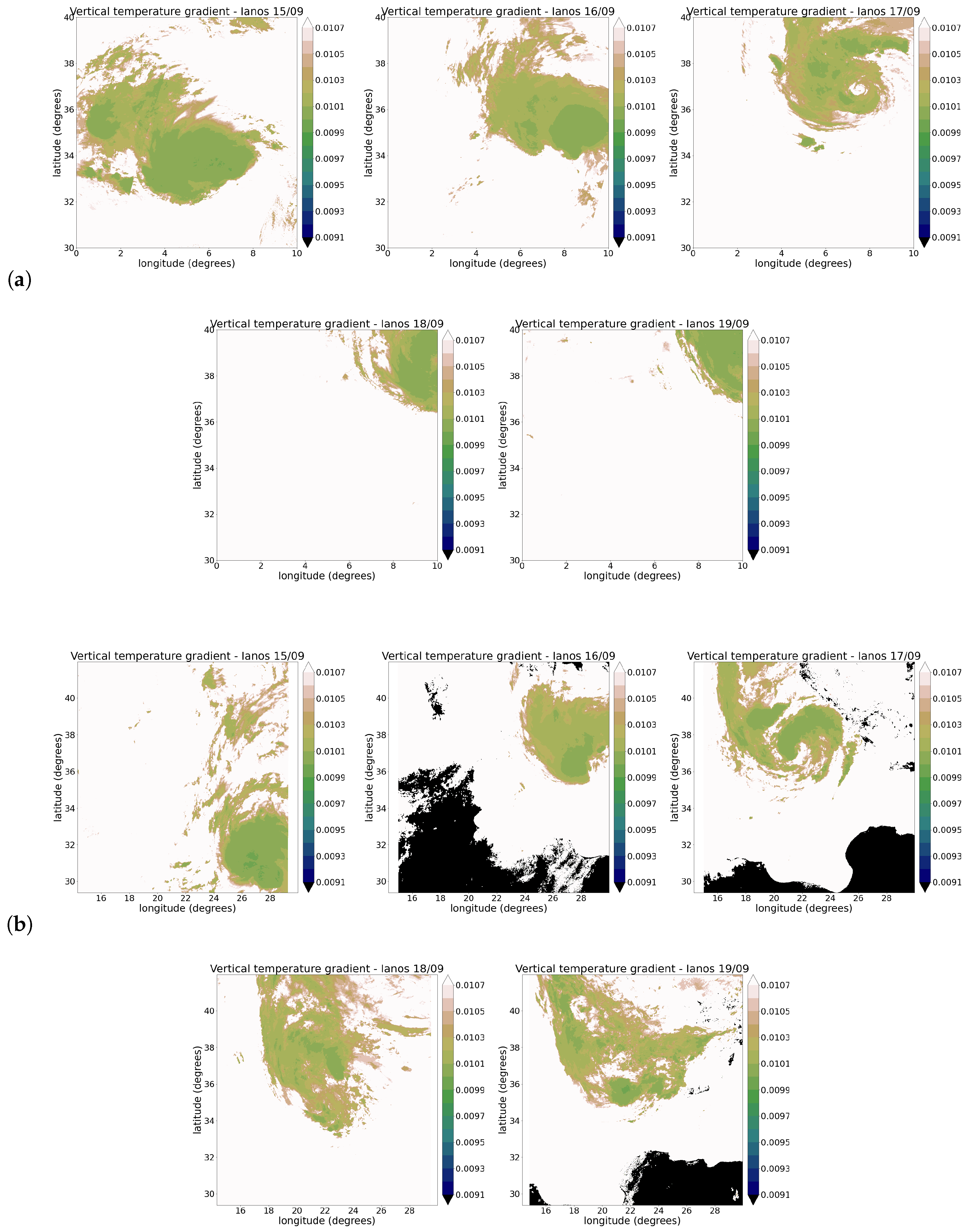
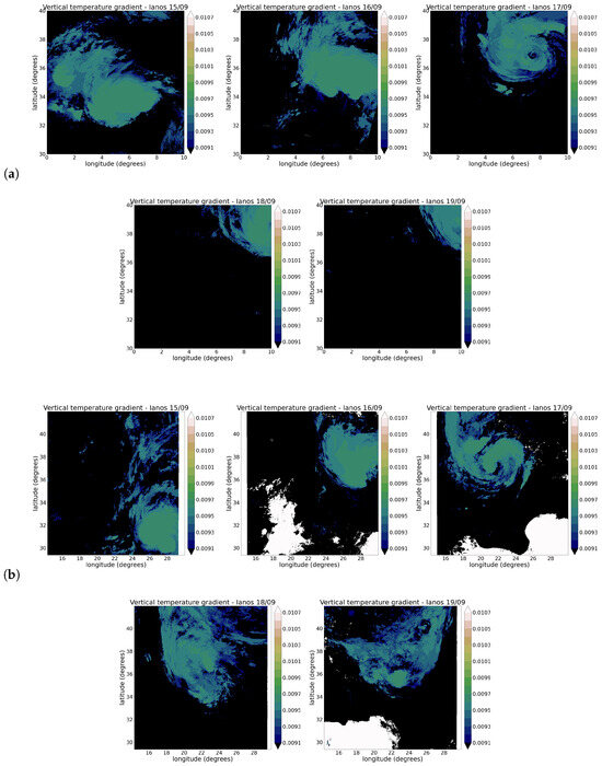
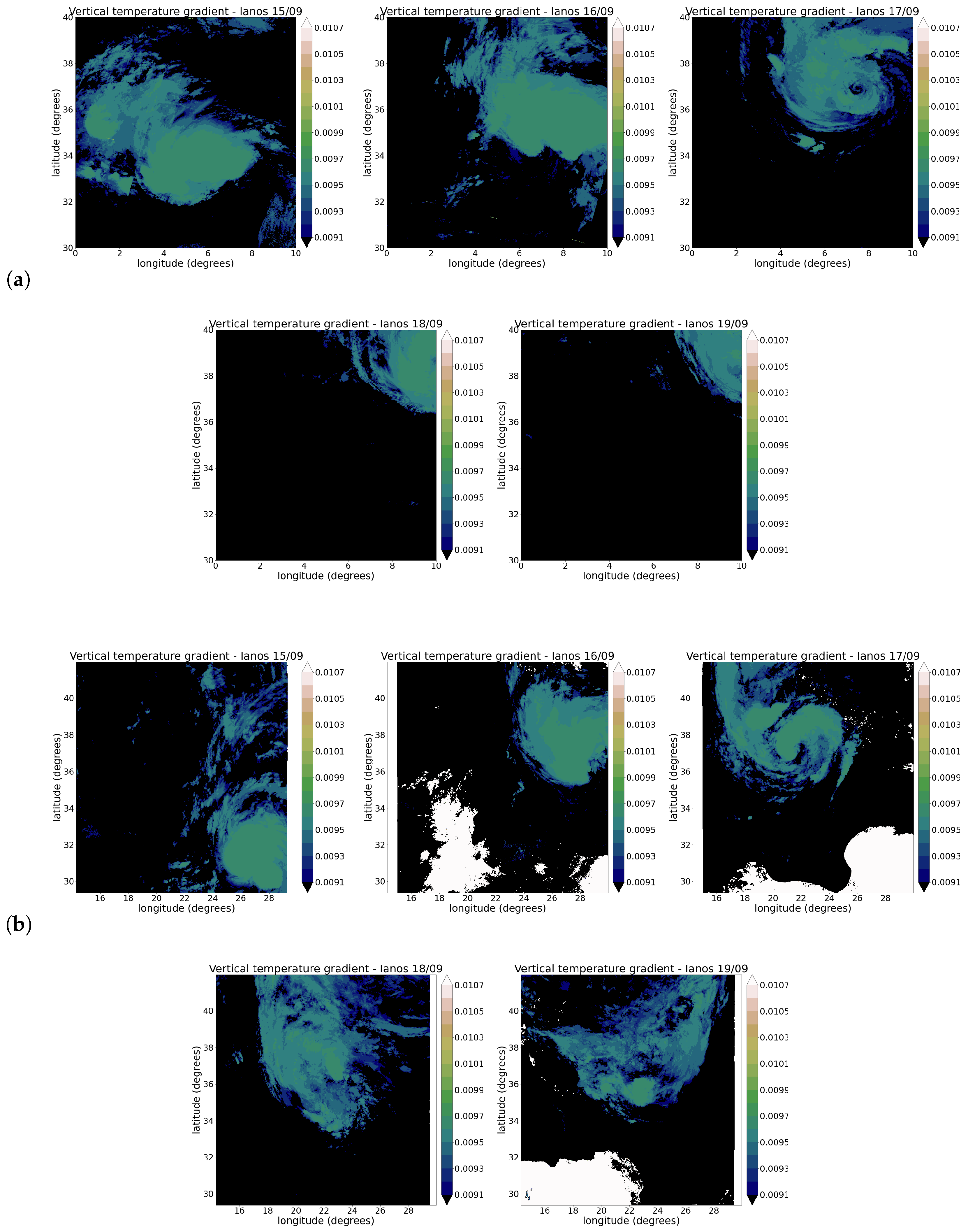
We perform this first assessment starting from the data from the VIIRS and SLSTR TIR spectral channels. The H and parameters, by fixing the daily value of , are used for computing and assessing atmospheric instability. More precisely, the vertical gradient is reported in Figure 14, where the (a) and (b) panels show that the values identify atmospheric instability throughout Ianos’s life days, from the daily values of BOLAM database. A further comparison can be carried out by looking at the values reported in Figure 15, where the panels contain the vertical gradient assessment, using daily values from the ERA5 database, instead. We remark that the information about this parameter is associated with what happens along the third dimension, although the vertical direction cannot be directly obtained from the satellite snapshots. However, it is firstly visible that the temperature gradient values show the overall conditions of absolute atmospheric instability within the cyclonic clouds ( K m−1 in all the scenes), from both the VIIRS and SLSTR products. The main difference between the values of the cloud systems is very slight when the daily snapshots obtained from BOLAM and ERA5 are compared ( K m−1 for BOLAM, with K m−1 for ERA5, on average, for all the images), while it is stronger when the background values are considered. In the maps of SLSTR products, some areas are affected by masks attributed to radiometric effects over the Earth’s surface pixels. These are identified with a white colour in the maps marked with ERA5 data and in a black colour in the BOLAM-based maps. Here, the values are very close to K m−1, in which the land surface temperature and the cloud-top temperature are mostly coincident.
Figure 14.
From left to right: temporally ordered scenes, from the 15th day to the 19th day of September, of the vertical gradient’s daily evolution for Ianos, observed by VIIRS (a) and SLSTR (b). is here taken from the daily values of the BOLAM database.
Figure 15.
From left to right: temporally ordered scenes, from the 15th day to the 19th day of September, of the vertical gradient’s daily evolution for Ianos, observed by VIIRS (a) and SLSTR (b). is here taken from the daily values of the ERA5 database.
3.6. Ianos Daily Evolution: Pressure Trend Around the Warm Core
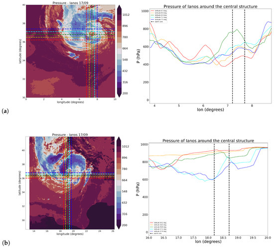
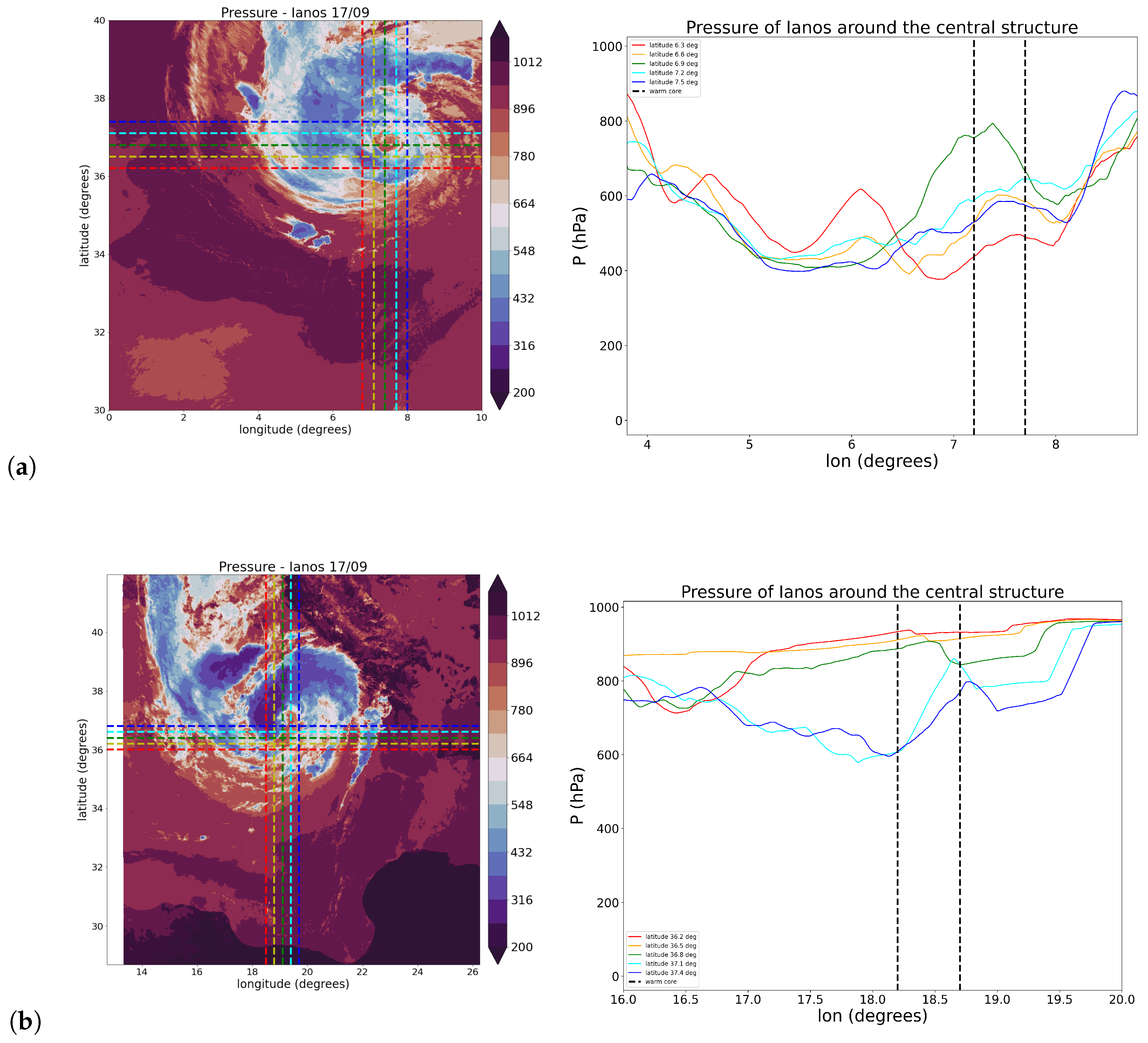
To estimate pressure trends in the products derived from the two sensors, the previously introduced exponential law is applied. A comparison between VIIRS and SLSTR imagery is performed by analysing the longitudinal pressure profiles of Ianos at several latitude bands surrounding the cyclone’s core. This is emphasised in Figure 16, where the spatial pressure distributions highlight the values near the eyewall. A characterisation of the minimum sea-level pressure (MSLP), extracted from both VIIRS and SLSTR products, enables the identification of the pressure within the eye of the cyclone through a daily comparison with recorded MSLP values from BOLAM and ERA5. To ensure a physically consistent comparison between satellite-retrieved and model-derived pressure diagnostics, warm-core pressure statistics are evaluated over a well-defined core region. The cyclone centre is diagnosed from MSLP at time t, consistently with the centre used in Figure 16. The core region is defined as the circular area bounded by the dashed reference radius shown, such that
where corresponds to the reference distance indicated by the dashed contour, latitude and longitude coordinates of the distance d. In all the days, the region corresponds to the number of gridpoints marked with the dashed lines in the figure ( pixels). The same points are considered in the compared values from BOLAM and ERA5. This approach provides a qualitative assessment of warm-core detection on the day of maximum intensification. The resulting indicators are reported in Table 3, in which the median values and the interquartile range are used to provide a robust measure of near-core pressure heterogeneity that is less sensitive to outliers than isolated extrema. These values are not intended to represent absolute MSLP estimates but, rather, to illustrate the relative evolution, spatial coherence, and persistence of the warm-core signature throughout the Ianos lifecycle. The comparison with the ERA5 and BOLAM MSLP fields is, therefore, framed as a qualitative consistency check, rather than a pointwise validation.
Figure 16.
The pressure field representation, with a focus on the pressure spatial trend around the central warm core of Ianos, from the VIIRS (a) and SLSTR (b) products of the 17th day. The colours of the lines in the left-panel plots correspond to the horizontal lines of the right-panel views.
Table 3.
The warm-core pressure statistics within the core region for the five-day lifecycle of Ianos. For each dataset and day, median values of MSLP are computed for pixels in the defined region. Values are reported with an interquartile range (IQR) in brackets and expressed in hPa units.
To further assess the internal consistency of the retrieval framework, BOLAM vertical temperature profiles within the warm-core region are reported in Table 4, following the same spatial averaging adopted for the pressure proxy. This comparison does not represent a quantitative calibration, but it provides a closed-loop consistency check between cloud-top-derived diagnostics and reanalysis-based thermodynamic profiles.
Table 4.
The warm-core temperature statistics within the core region for the five-day lifecycle of Ianos. For each dataset and day, median values of temperature are computed for pixels in the defined region. Values are reported with an interquartile range (IQR) in brackets and expressed in K units.
4. Discussion
This work provides an integrated multiscale characterisation of the Ianos TLC by combining spatio-temporal and remote-sensed analyses from GEO and LEO satellites, respectively. The methodology demonstrates that POD is a powerful diagnostic tool for extracting coherent structures, quantifying their energy content, and disentangling the spatial and temporal variability governing the evolution of Mediterranean TLCs. The POD applied to SEVIRI-derived temperature and pressure fields shows that a limited subset of modes captures most of the system’s variability, indicating the presence of persistent, energetically dominant structures. Large-scale modes describe the synoptic organisation and rotational symmetries of the warm-core system, whereas intermediate and small-scale modes highlight convective filaments and localised gradients dynamically linked to the intensification phase. The scale-dependent reconstructions confirm that the strongest signatures of tropical transition manifest in the intermediate scales, where the spectra display a nearly power-law behaviour. The latter seems to be consistent with a forward energy cascade in a strongly stratified fluid, as described in the context of mesoscale and stratified turbulence, despite the characteristic marked differences between the compared events. Particularly, spatial spectral slopes of Ianos and the TCs ones can be understood as a consequence of the confined Mediterranean basin and the stronger baroclinic environment in which tropical-like cyclones develop. These factors limit the horizontal scale separation and effectively truncate or modify the inertial-range-like behaviour compared to oceanic tropical cyclones. Inversely, the slopes of the temporal spectra exhibit comparability, according to the dominance of convective life-cycle variability (order of ∼30–60 min) and intermittent diabatic processes, which are less sensitive to basin size and act similarly in both environments. In addition, given the strongly rotating and stratified environment, part of this variability captured through POD may reflect inertial–gravity wave activity and wave–convection coupling. While a quantitative separation between balanced and unbalanced motions is beyond the scope of the present diagnostics, the observed spatio-temporal organisation is consistent with mixed contributions from coherent convective structures and wave-like variability.
It has to be taken into account that the analysis tends to investigate the multiscale statistical structure of observation–background departures for Ianos, without aiming to assess the cumulative impact of data assimilation on the full model state evolution. Within this framework, the POD decomposition provides a scale-resolved description of the dynamical features captured by the satellite observations, which can be interpreted in terms of the multiscale characteristics of the event. Furthermore, POD results indicate differences in spatial organisation between the Mediterranean and the ocean, while the convective dynamics highlight the comparable persistence in their temporal variability.
The comparison of POD spectra across the formation, peak, and weakening stages reveals a systematic redistribution of energy toward smaller scales during the mature phase, indicative of enhanced convective activity and coherent turbulent-like organisation of the cloud field. Accordingly, the DCCP mask, derived from combined TIR–WV constraints, leads to the presence of a compact, spiral-shaped convective core during maximum intensity, consistent with a fully developed warm-core structure. In particular, in the recent framework, the identification of a fully tropical phase requires quantitative thresholds with a high degree of convective symmetry [19]. The DCCP analysis is not intended as a quantitative validation of convective intensity but as a complementary structural diagnostic supporting the multiscale interpretation derived from the POD analysis. These results indicate that Ianos developed pronounced tropical-like features, during its mature phase, despite these features seeming to be influenced by the transition of a mixed baroclinic–diabatic environment. As such, our findings satisfy the enhanced tropicality of the WMO criteria. Compared with existing TC-POD studies, in this application, the temporal energy spectra exhibit slopes comparable to those reported for tropical cyclones. A cross-comparison with tropical cyclones Faraji and Freddy shows that, while the spectral shape is broadly analogous, Ianos exhibits different slope values across spatial and temporal ranges. The analysis indicates that the spatial spectra, while retaining some similarities with tropical systems, exhibit marked differences in the scaling behaviour. We attribute this phenomenon to the fact that Mediterranean TLCs develop within a confined basin, under strong baroclinic forcing. In this sense, the POD analysis provides new insight into how multiscale energy cascades can be modified in these events, tending to highlight the role of environmental constraints and mixed baroclinic–diabatic processes. Furthermore, the similarity of temporal spectral slopes is consistent with WISHE-type feedbacks, which regulate convective growth rates largely independent of the basin size, whereas the altered spatial slopes reflect the reduced horizontal extent and the stronger stratification. This interpretation can be attributed to a truncated or modified energy cascade, compared to tropical cyclones at the maximum intensity. Moreover, one should take into account that the maximum intensity of a Medicane corresponds to a very different intensity stage, in the case of a hurricane.
The LEO-based daily analysis further confirms the tropical-like thermodynamic structure: the vertical temperature gradients consistently exceed the dry-adiabatic threshold ( 0.01 K m2), indicating daily persistence for absolute instability within the cloud system. Pressure intervals of values exhibit a coherent warm-core signature over all days and the persistence and spatial coherence of the warm-core minimum support the use of cloud-top-based pressure proxies as qualitative indicators of cyclone structure.
5. Conclusions
The analysed framework tends to highlight that the use of the POD analysis is based on capturing the multiscale organisation of thermodynamic anomalies and convective structures. While the absolute values of retrieved temperature and pressure may be affected by simplified assumptions, the scale-dependent spectral properties and coherent patterns remain robust indicators of the underlying dynamical organisation.
Overall, this study demonstrates that integrating POD with multi-sensor satellite data provides a robust and physically grounded framework for diagnosing the multiscale energetics of Medicanes. The approach is focused on persistent coherent structures and transient convective contributions, offering new perspectives for the remote-sensing-based monitoring of Mediterranean TLCs, even starting from cyclogenetic lows.
Future work should further investigate the multiscale structure of POD-derived spectra by attributing their energetic behaviour to specific atmospheric processes involved in these extreme events, such as baroclinic triggering, tropical transition, and warm-core maintenance, as well as by exploiting additional multi-sensor spectral channels new thermodynamic and microphysical advanced characterisations. In order to redefine instability metrics, mesoscale vorticity proxies, or pressure perturbation indicators would be exploited with high-resolution numerical simulations dedicated to TLC dynamics. Such coupling between observational multiscale analyses and modelling frameworks will improve their interpretation, validation, and prediction.
Supplementary Materials
The following supporting information can be downloaded at: https://www.mdpi.com/article/10.3390/rs18040602/s1.
Author Contributions
Conceptualisation, V.C. and F.F.; methodology, G.C. and L.P.; software, G.C. and L.P.; validation, V.C., F.F. and F.L.; formal analysis, G.C. and L.P.; investigation, G.C.; resources, G.C. and F.F.; data curation, G.C. and F.F.; writing—original draft preparation, G.C. and L.P.; writing—review and editing, F.L.; visualisation, G.C.; supervision, L.P. and F.L.; project administration, F.F. and V.C. All authors have read and agreed to the published version of the manuscript.
Funding
G.C. and F.L. have been supported by the Space It Up project funded by the Italian Space Agency, ASI, and the Ministry of University and Research, MUR, under contract n. 2024-5-E.0—CUP n. I53D24000060005. G.C. has also been supported by the Italian “Ministero dell’Università e della Ricerca” (MUR) under the program PON “Ricerca e Innovazione” 2014–2020, Azione IV.5—“Dottorati su tematiche green” tematica “Cambiamento climatico e accelerazione di eventi estremi nel bacino del Mediterraneo”.
Institutional Review Board Statement
Not applicable.
Informed Consent Statement
Not applicable.
Data Availability Statement
Data elaborated in the present article were downloaded from the following sites (last accessed on 11 February 2025): https://view.eumetsat.int/productviewer?v=default, by selecting “Meteosat-8 41.5 E” for “satellite”, “High Rate SEVIRI IR10.8—MSG—Indian Ocean” for “Channels”. https://ladsweb.modaps.eosdis.nasa.gov, “VIIRS Suomi NPP”—“SLSTR ESA Copernicus Sentinel-3A”—“SLSTR ESA Copernicus Sentinel-3” for “Sensors”, “VNP41A1”—“S3ASL1RBT”—“S3BSL1RBT” for “Products”.
Acknowledgments
L.P. acknowledges the contribution received from “Fondo per il Programma Nazionale di Ricerca e Progetti di Rilevante Interesse Nazionale (PRIN)” under the project “TURBIMECs: study of TURBulence In MEditerranean Cyclone events”, grant n. 2022S3RSCT, CUP Master B53D23007500006.
Conflicts of Interest
The authors declare no conflict of interest.
Abbreviations
The following abbreviations are used in this manuscript:
| MSG-11 | Meteosat Second Generation 11 |
| POD | Proper Orthogonal Decomposition |
| SEVIRI | Spinning Enhanced Visible Infra-Red Imager |
| 2D FFT | Two-Dimensional Fast Fourier Transform |
| LEO | Low Earth Orbit |
| SLSTR | Sea and Land Surface Temperature Radiometer |
| Suomi NPP | Suomi National Polar-Orbiting Partnership |
| VIIRS | Visible/Infrared Imager Radiometer Suite |
References
- Ernst, J.; Matson, M. A Mediterranean tropical storm? Weather 1983, 38, 332–337. [Google Scholar] [CrossRef] [Scilit]
- Billing, H.; Haupt, I.; Tonn, W. Evolution of a hurricane-like cyclone in the Mediterranean sea. Beiträge zur Physik der Atmosphäre 1983, 56. Available online: https://api.semanticscholar.org/CorpusID:132679071 (accessed on 11 February 2026).
- Emanuel, K.A. Genesis and Maintenance of “Mediterranean hurricanes”. Adv. Geosci. 2005, 2, 217–220. [Google Scholar] [CrossRef] [Scilit]
- Miglietta, M.M. Mediterranean Tropical-like Cyclones (Medicanes). Atmosphere 2019, 10, 206. [Google Scholar] [CrossRef] [Scilit]
- Hatzaki, M.; Flaounas, E.; Davolio, S.; Pantillon, F.; Patlakas, P.; Raveh-Rubin, S.; Hochman, A.; Kushta, J.; Khoyadar, S.; Dafis, S.; et al. Working together understanding Mediterranean Cyclones. Bull. Am. Meterol. Soc. 2023, 104, E480–E487. [Google Scholar] [CrossRef] [Scilit]
- Flaounas, E.; Davolio, S.; Raveh-Rubin, S.; Pantillon, F.; Miglietta, M.M.; Gaertner, M.A.; Hatzaki, M.; Homar, V.; Khodayar, S.; Korres, G.; et al. Mediterranean Cyclones: Current Knowledge and Open Questions on Dynamics, Prediction, Climatology and Impacts. Weather Clim. Dyn. 2022, 3, 173–208. [Google Scholar] [CrossRef] [Scilit]
- Moscatello, A.; Miglietta, M.M.; Rotunno, R. Numerical Analysis of a Mediterranean “Hurricane” over Southeastern Italy. Mon. Weather Rev. 2008, 136, 4373–4397. [Google Scholar] [CrossRef] [Scilit]
- Romero, R.; Emanuel, K.A. Medicane risk in a changing climate. J. Geophys. Res. Atmos. 2013, 118, 5992–6001. [Google Scholar] [CrossRef] [Scilit]
- Cavicchia, L.; Von Storch, H.; Gualdi, S. Mediterranean Tropical-Like Cyclones in Present and Future Climate. J. Clim. 2014, 27, 7493–7501. [Google Scholar] [CrossRef] [Scilit]
- Miglietta, M.M.; Rotunno, R. Development Mechanisms in Mediterranean Tropical-like Cyclones (Medicanes). Q. J. R. Meteorol. Soc. 2019, 145, 1444–1460. [Google Scholar] [CrossRef] [Scilit]
- Mazza, E.; Ulbrich, U.; Klein, R. The Tropical Transition of the October 1996 Medicane in the Western Mediterranean Sea: A Warm Seclusion Event. Mon. Weather Rev. 2017, 145, 2575–2595. [Google Scholar] [CrossRef] [Scilit]
- Fita, L.; Flaounas, E. Medicanes as Subtropical Cyclones: The December 2005 case from the Perspective of Surface Pressure Tendency Diagnostics and Atmospheric Water Budget. Q. J. R. Meteorol. Soc. 2018, 144, 1028–1044. [Google Scholar] [CrossRef] [Scilit]
- Emanuel, K.A. An Air-sea Interaction Theory for Tropical Cyclones Part I: Steady-state maintenance. J. Atmos. Sci. 1986, 43, 585–605. [Google Scholar] [CrossRef] [Scilit]
- Lagouvardos, K.; Kotroni, V.; Nickovic, S.; Jovic, D.; Kallos, G.; Tremback, C.J. Observations and Model Simulations of a Winter Sub-synoptic Vortex over the Central Mediterranean. Meteorol. Appl. 1999, 6, 371–383. [Google Scholar] [CrossRef] [Scilit]
- Fita, L.; Romero, R.; Ramis, C. Intercomparison of Intense Cyclogenesis Events over the Mediterranean Basin Based on Baroclinic and Diabatic Influences. Adv. Geosci. 2006, 7, 333–342. [Google Scholar] [CrossRef] [Scilit]
- Comellas Prat, A.; Federico, S.; Torcasio, R.C.; D’Adderio, L.P.; Dietrich, S.; Panegrossi, G. Evaluation of the Sensitivity of Medicane Ianos to Model Microphysics and Initial Conditions Using Satellite Measurements. Remote Sens. 2021, 13, 4984. [Google Scholar] [CrossRef] [Scilit]
- Dafis, S.; Claud, C.; Kotroni, V.; Lagouvardos, K.; Rysman, J. Insights into the Convective Evolution of Mediterranean Tropical-like Cyclones. Q. J. R. Meteorol. Soc. 2020, 146, 4147–4169. [Google Scholar] [CrossRef] [Scilit]
- Wieczorek, A. Medicanes—The hurricanes of Mediterranean? Wetterdienst Thema Des Tages 2015, 1. [Google Scholar]
- Gutiérrez-Fernández, J.; Miglietta, M.M.; González-Alemán, J.J.; Gaertner, M.A. A new refinement of Mediterranean tropical-like cyclones characteristics. Geophys. Res. Lett. 2024, 51, e2023GL106429. [Google Scholar] [CrossRef] [Scilit]
- Panegrossi, G.; D’Adderio, L.P.; Dafis, S.; Rysman, J.; Casella, D.; Dietrich, S.; Sanò, P. Warm Core and Deep Convection in Medicanes: A Passive Microwave-Based Investigation. Remote Sens. 2023, 15, 2838. [Google Scholar] [CrossRef] [Scilit]
- Ciardullo, G.; Primavera, L.; Ferrucci, F.; Lepreti, F.; Carbone, V. A Satellite Analysis: Comparing Two Medicanes. Atmosphere 2024, 15, 481. [Google Scholar] [CrossRef] [Scilit]
- Hong, G.; Heygster, G.; Rodriguez, C.A.M. Effect of cirrus clouds on the diurnal cycle of tropical deep convective clouds. J. Geophys. Res. 2006, 111, D06209. [Google Scholar] [CrossRef] [Scilit]
- Wu, Q.; Ruan, Z. Diurnal variations of the areas and temperatures in tropical cyclone clouds. Q. J. R. Meteorol. Soc. 2016, 142, 2788–2796. [Google Scholar] [CrossRef] [Scilit]
- Ciardullo, G.; Primavera, L.; Ferrucci, F.; Lepreti, F.; Carbone, V. New Investigation of a Tropical Cyclone: Observational and turbulence analysis for the Faraji Hurricane. Remote Sens. 2023, 15, 1383. [Google Scholar] [CrossRef] [Scilit]
- Ciardullo, G.; Primavera, L.; Ferrucci, F.; Lepreti, F.; Carbone, V. Remote Sensed Spatio-temporal Study of Tropical Cyclone Freddy Exceptional Case. Remote Sens. 2025, 17, 981. [Google Scholar] [CrossRef] [Scilit]
- Lagouvardos, K.; Karagiannidis, A.; Dafis, S.; Kalimeris, A.; Kotroni, V. Ianos—A Hurricane in the Mediterranean. Bull. Am. Meteorol. Soc. 2022, 103, E1621–E1636. [Google Scholar] [CrossRef] [Scilit]
- Ciardullo, G.; Primavera, L.; Ferrucci, F.; Carbone, V.; Lepreti, F. Study of turbulence associated with the Faraji Cyclone. Climate 2022, 10, 21. [Google Scholar] [CrossRef] [Scilit]
- Vecchio, A.; Carbone, V.; Lepreti, F.; Primavera, L.; Sorriso-Valvo, L.; Veltri, P.; Straus, T.; Alfonsi, G. Proper Orthogonal Decomposition of Solar Photospheric Motions. Phys. Rev. Lett. 2005, 95, 061102. [Google Scholar] [CrossRef] [Scilit]
- Siegel, S.G.; Cohen, K.; Seidel, J.; McLaughlin, T. Proper Orthogonal Decomposition Snapshot Selection for State Estimation of Feedback Controlled Flows. In Proceedings of the 44th AIAA Aerospace Sciences Meeting and Exhibit, Reno, NV, USA, 9–12 January 2006; pp. 1–11. [Google Scholar] [CrossRef] [Scilit]
- Vecchio, A.; Carbone, V.; Lepreti, F.; Primavera, L.; Sorriso-Valvo, L.; Straus, T.; Veltri, P. Spatio-Temporal Analysis of Photospheric Turbulent Velocity Fields Using the Proper Orthogonal Decomposition. Sol. Phys. 2008, 251, 163–178. [Google Scholar] [CrossRef] [Scilit]
- Lumley, J.L. Coherent Structures in Turbulence. Transition and Turbulence; Academic Press: New York, NY, USA, 1981. [Google Scholar]
- Berkooz, G.; Holmes, P.; Lumley, J.L. The Proper Orthogonal Decomposition in the Analysis of Turbulent Flows. Annu. Rev. Fluid Mech. 1993, 25, 539–575. [Google Scholar] [CrossRef]
- Alfonsi, G.; Restano, C.; Primavera, L. Coherent structures of the flow around a surface-mounted cubic obstacle in turbulent channel flow. J. Wind Eng. Ind. Aerodyn. 2003, 91, 495–511. [Google Scholar] [CrossRef] [Scilit]
- Alfonsi, G.; Primavera, L.; Felisari, R. On the behavior of POD modes of the flow past a perforated plate. J. Flow Vis. Image Process. 2003, 10, 105–117. [Google Scholar] [CrossRef] [Scilit]
- Alfonsi, G.; Primavera, L. The structure of turbulent boundary layers in the wall region of plane channel flow. Proc. R. Soc. A 2007, 463, 593–612. [Google Scholar] [CrossRef] [Scilit]
- Lindborg, E. The energy cascade in a strongly stratified fluid. J. Fluid Mech. 2006, 550, 207–242. [Google Scholar] [CrossRef] [Scilit]
- Salby, M.L. Fundamental of Atmospheric Physics; Academic Press: London, UK, 1996. [Google Scholar]
- Ahrens, C.D. Meteorology Today: An Introduction to Weather, Climate, and the Environment, 9th ed.; Brooks/Cole, CengageLearning: Boston, MA, USA, 2009. [Google Scholar]
- Mapes, B.E.; Houze, R.A. Cloud Clusters and Superclusters over the Oceanic Warm Pool. Mon. Weather Rev. 1993, 121, 1398–1416. [Google Scholar] [CrossRef] [Scilit]
- Kolat, U.; Menzel, W.P.; Olson, E.; Frey, R. Very high cloud detection in more than two decades of HIRS data. J. Geophys. Res. Atmos. 2013, 118, 3278–3284. [Google Scholar] [CrossRef] [Scilit]
- Setvak, M.; Rabin, R.M.; Wang, P.K. Contribution of the MODIS instrument to observations of deep convective storms and stratospheric moisture detection in goes and MSG imagery. Atmos. Res. 2007, 83, 505–518. [Google Scholar] [CrossRef] [Scilit]
- Olander, T.L.; Velden, C.S. The Advanced Dvorak Technique: Continued development of an objective scheme to estimate tropical cyclone intensity using geostationary infrared satellite imagery. Weather Forecast. 2007, 22, 287–298. [Google Scholar] [CrossRef] [Scilit]
- Kotarba, A.Z.; Wojciechowska, I. Satellite-based detection of deep convective clouds: The sensitivity of infrared methods, and implications for cloud climatology. Atmos. Meas. Tech. 2024, 18, 2721–2738. [Google Scholar] [CrossRef] [Scilit]
- Buzzi, A.; Fantini, M.; Malguzzi, P.; Nerozzi, F. Validation of a limited area model in cases of Mediterranean Cyclogenesis: Surface fields and precipitation scores. Meteorol. Atmos. Phys. 1994, 53, 137–153. [Google Scholar] [CrossRef] [Scilit]
- Orlandi, E.; Fierli, F.; Davolio, S.; Buzzi, A.; Drofa, O. A nudging scheme to assimilate satellite brightness temperature in meteorological model: Impact on representation of African Mesoscale Convective Systems. Q. J. R. Meteorol. Soc. 2010, 136, 462–474. [Google Scholar] [CrossRef] [Scilit]

Disclaimer/Publisher’s Note: The statements, opinions and data contained in all publications are solely those of the individual author(s) and contributor(s) and not of MDPI and/or the editor(s). MDPI and/or the editor(s) disclaim responsibility for any injury to people or property resulting from any ideas, methods, instructions or products referred to in the content. |
© 2026 by the authors. Licensee MDPI, Basel, Switzerland. This article is an open access article distributed under the terms and conditions of the Creative Commons Attribution (CC BY) license.