


Highlights
What are the main findings?
- RSGP: A synthesis framework for core RS challenges.
- BME is the core of the remote sensing geostatistical paradigm.
What are the implications of the main findings?
- The concept of soft data provides a universal interface for estimation and mapping.
- Quantifying spatiotemporal correlation absorbs inherent data structure.
Abstract
Advancements in earth observation technologies are ushering in the big data era, yet this potential is compromised by intrinsic challenges: inherent uncertainty, spatiotemporal heterogeneity, multi-scale character, and pervasive data gaps. Traditional methods often fail to address these issues within a single, coherent system. The main contributions of this review are to systematically establish the Remote Sensing Geostatistical Paradigm (RSGP) as a comprehensive, unified framework. Powered by its core theory, Bayesian Maximum Entropy (BME), RSGP is a broadly designed epistemic framework that transcends a mere conceptual reorganization of established methods. It addresses the above challenges by highlighting two pivotal concepts within a spatiotemporal random field: (1) uncertainty quantification via probabilistic soft data, which redefines observations as probability density functions, representing a fundamental epistemological shift from deterministic scalars to probabilistic entities, and provides a universal interface for rigorous assimilation of heterogeneous remote sensing or in situ observations and synergy with other computational models, such as machine learning; and (2) spatiotemporal structure exploitation, which integrates the underlying structure embedded in remote sensing data of natural attributes, moving beyond mere optical properties to incorporate a broader range of available spatiotemporal information, for robust estimation and mapping purposes. Furthermore, the evolution of key technologies is illustrated by using real-world application cases, guiding how to implement RSGP in terms of different scenarios. Finally, the paradigm’s features and limitations are discussed. This synthesis provides the remote sensing community with a robust foundation for uncertainty-aware analysis and multi-source integration, bridging geostatistical logic with next-generation AI-driven Earth observation.
1. Introduction
Advancements in earth observation technologies are ushering in the big data era, driven by the emergence of diverse satellites and the advanced sensors they carry [1,2,3]. Notably, prolific sensors like MODIS (Moderate-resolution Imaging Spectroradiometer) and those from the Landsat and Sentinel programs are at the forefront of this data revolution. These sensors enable the continuous monitoring of the environment, ecology, natural resources, and climate across vast spatial and temporal scales [4,5,6,7]. Such monitoring provides access to previously inaccessible data, thereby unlocking unprecedented opportunities for gaining novel insights into the complex dynamics of natural and socioeconomic systems.
1.1. Challenges in Earth Observation Data
Realizing the full potential of this data deluge is often compromised by inherent challenges. A primary one is the pervasive issue of missing or contaminated data, and reliable satellite observations are inevitably incomplete. This is frequently caused by obstructions such as cloud cover, cloud shadows, and sun glint, as well as by sensor-specific malfunctions [8,9,10], see Figure 1a. Compounding the challenge of data gaps, a second fundamental issue arises from the inherent design trade-offs of satellite sensors, leading to significant inconsistencies in spatiotemporal resolution. This presents a persistent dilemma for researchers. Sensors like MODIS own high temporal resolution imagery (1–2 days), but at a coarse spatial resolution (250 m–1 km); conversely, the high-resolution images obtained from Sentinel-2 or Landsat 8 have much longer revisit times (10–16 days) [11]. This trade-off is further nuanced by constellations like PlanetScope; while they offer an exceptionally fine spatial resolution (3 m), they are constrained by a very narrow swath width (24.6 km) [12]. This inherent heterogeneity in spatiotemporal resolution makes the task of fusing multi-source data a formidable challenge, which is a crucial step toward creating a coherent and complete picture of Earth’s systems [13]; see Figure 1b,c. Finally, a third fundamental issue is the inherent uncertainty propagated throughout the remote sensing chain. The initial signal is imperfect, as it is attenuated and scattered by atmospheric particles [14,15]. This physical uncertainty is then compounded by the retrieval algorithms, which are themselves imperfect models built on various assumptions [16]; see Figure 1d. Consequently, the final data product is not an absolute truth but an estimate, which inevitably inherits complex, propagated uncertainty from both the signal and the model. These cumulative limitations can ultimately distort the accurate characterization of natural systems, thereby weakening the reliability of scientific insights derived from them.
Figure 1.
Conceptual illustration of the three core challenges inherent in remote sensing data: (a) pervasive data gaps caused by obstructions (e.g., clouds in the southeastern part, image from Sentinel-2 on 4 January 2025); (b,c) spatiotemporal heterogeneity, illustrated by the trade-off between a Sentinel-2 image (10 m spatial resolution, 10-day temporal resolution) and a Landsat 8 image (30 m spatial resolution, 16-day temporal resolution) from the same date (3 July 2024); and (d) inherent uncertainty (discrepancies between remote estimates and in situ ground truth).
1.2. From Traditional Geostatistics to Bayesian Maximum Entropy
In order to address these issues, geostatistical approaches exhibit an advantage of using known spatiotemporal neighbors to estimate values at unsampled locations. Specifically, the field of geostatistics presents a rigorous mathematical framework for analyzing spatially and spatiotemporally regionalized variables [17,18]. Originating in mining geology, geostatistics is fundamentally built upon Tobler’s First Law of Geography (TFLG), which states that “everything is related to everything else, but near things are more related than distant things”. It operationalizes this concept by using the covariance or variogram to quantify this spatial or spatiotemporal correlation for natural attribute estimation and mapping purposes [19,20,21]. Historically, the most popular implementation of this principle is the Kriging family of techniques [17]. However, classical Kriging faces deficiencies. It is structurally confined to handling only first- and second-order statistical moments (i.e., mean and covariance) and lacks the capacity to integrate other valuable knowledge bases, such as physical laws or conceptual models. Furthermore, it offers only limited results for incorporating uncertain data in a precise and efficient manner [22]. Ultimately, these structural constraints preclude the rigorous assimilation of complex physical laws, non-Gaussian or uncertain data, all of which are prevalent in the remote sensing domain.
The modern spatiotemporal geostatistical methodology, Bayesian Maximum Entropy (BME), was developed specifically to overcome these constraints. Conceptually, BME serves as a knowledge-based integration engine, offering a rigorous framework for integrating two types of information: general knowledge (e.g., physical laws, high-order moments, expert judgment) and site-specific knowledge (including both precise hard data and uncertain soft data) [23,24]. Critically, BME achieves this without relying on the restrictive assumptions (e.g., Gaussianity, linearity) that can limit traditional Kriging, thus affording a more flexible and potentially more accurate approach for complex data and attribute systems estimation and mapping [25]. This conceptual role makes BME well-suited for remote sensing data reconstruction, fusion, and parameter retrieval as it effectively bridges the gap between fragmented satellite observations and underlying continuous natural processes. Specifically, the capacity to integrate soft data is the key, which is formally represented using probability density functions (PDFs). For instance, this allows coarse-resolution (or less accurate) data to be treated as soft data, while fine-resolution (or more accurate) data are simultaneously treated as hard data [26,27]. Applying BME reveals a fundamental enhancement: while the original remote sensing products primarily represent the attribute’s optical characteristics, BME additionally assimilates the attribute’s inherent spatiotemporal correlation characteristics, thereby systematically reducing estimation and mapping uncertainty and yielding a final product that is demonstrably more robust [16]. Consequently, BME serves as a vital synthesis engine that reconciles the fragmented and uncertain nature of Earth observation with the requirement for rigorous, physically consistent environmental mapping.
1.3. Emergence of the Remote Sensing Geostatistical Paradigm
In this sense, the Remote Sensing Geostatistical Paradigm (RSGP) can be formally defined as a comprehensive methodological and applied framework that treats remote sensing data as regionalized variables, leveraging geostatistical theory for spatiotemporal modeling, optimal estimation, multi-scale transformation/fusion, and uncertainty assessment. This paradigm, therefore, provides a fundamentally new epistemology by shifting the focus from deterministic scalar observations to probabilistic information synthesis. Conceptually, it differs from traditional Bayesian geostatistics by using the Maximum Entropy principle to derive objective priors from general knowledge, and it distinguishes itself from model-driven Data Assimilation (DA) by being information-driven. While DA typically relies on explicit dynamic forward models to update states, RSGP prioritizes the exploitation of inherent spatiotemporal structural dependencies within the data itself, offering a more flexible solution when dynamic physical equations are incomplete or unavailable.
Furthermore, the RSGP transcends traditional remote sensing inversion and data fusion by formalizing spatiotemporal continuity. While conventional inversion is typically pixel-wise and often neglects spatial dependencies, the RSGP treats these inversion outputs as probabilistic soft data refined through spatiotemporal random field logic [16]. Similarly, whereas traditional fusion relies on deterministic resampling that may distort uncertainty structures, the RSGP provides a rigorous Bayesian synthesis. This ensures that multi-source integration remains physically and statistically consistent with both individual data uncertainties and the attribute’s inherent spatiotemporal structure.
Recent studies have provided comprehensive reviews on specific challenges such as multi-sensor data fusion and geostatistical simulation models [13,18]. Theoretical frameworks for handling geospatial big data have also been established [28]. Despite these advancements, existing literature often treats geostatistical logic and data-driven algorithms as isolated or fragmented domains. This study introduces the RSGP as a unified scientific architecture. It fills a critical gap in the literature by linking geostatistical techniques with high-performance inductive learning, serving as an integrative bridge between uncertainty quantification and data-driven inductive modeling. The added value of this paradigm lies in its ability to offer a universal interface (soft data) for harmonizing heterogeneous observations while providing a deductive governance framework that ensures the data-driven model predictions adhere to inherent spatiotemporal logic.
This review is organized as follows: Section 2 establishes the foundational theoretical and computational pillars of the paradigm, specifically the Spatiotemporal Random Field and BME. Section 3 traces the evolutionary trajectory of key technologies, ranging from fundamental interpolation to sophisticated multi-source assimilation and non-conventional applications. In Section 4, the unique characteristics, methodological advantages, and operational boundaries of the RSGP are critically summarized. Section 5 demonstrates the paradigm’s practical utility through diverse real-world case studies and implementation guidelines. Finally, Section 6 concludes with a summary of the paradigm’s contributions and a discussion of future research directions for this emerging field.
2. Foundational Concepts and Methodologies of the Paradigm
2.1. Spatiotemporal Random Field Model
The theoretical cornerstone of the RSGP is the Spatiotemporal Random Field (STRF) model [29]. STRF is a model that generally associates mathematical quantities with the points of a spatiotemporal continuum in conditions of uncertainty. It is conceptualized as a real-valued random function defined on a spatiotemporal domain, which is characterized by the intrinsic relationship between space and time. Consequently, the “random function” and the “spatiotemporal domain” constitute the two primary components of the STRF’s conceptual characterization.
In the context of remote sensing, the STRF model solves a fundamental conceptual problem: it shifts the perspective from viewing satellite observations as isolated, deterministic pixels to treating them as a set of stochastic, sparse, multi-scale, and uncertain samples of an underlying continuous natural process [16,30,31,32]. This model is specifically designed to study natural processes that, while often stochastic in character, exhibit spatial or spatiotemporal dependency operationalized by TFLG. Common examples include sea surface chlorophyll, land surface temperature, and aerosol optical depth, etc., all of which exhibit spatiotemporal dependency and evolve within the spatiotemporal continuum despite inherent remote sensing uncertainties [33,34,35].
In this model, a remotely observed natural process is represented as an STRF variable , which is a collection of random variables (RVs) at all point locations in the spatiotemporal domain . Each point comprises spatial coordinates (in an n-dimensional space ) and a temporal coordinate t (in a temporal domain ). Usually, n equals 2. From a stochastic viewpoint, an RV is fully described by its PDF, which in turn is defined by its statistical moments (e.g., mean, variance, variogram, and higher-order moments). These moments can be regarded as random functions mentioned above. Specifically, the mean function and covariance function representing the trends and the correlations/dependencies between two locations, respectively, are the two principal moments used to characterize an STRF in the paradigm [36]. Moreover, the semivariogram function is a functionally equivalent alternative to the covariance function for describing the spatiotemporal correlation structure. Under the assumption of spatiotemporal second-order stationarity, these two functions no longer depend on the absolute pair locations . Instead, the spatial distance , and temporal lag define the values of covariance and semivariogram, i.e., and ; furthermore, the two functions are directly interchangeable via the relationship , where is a constant value [37]. Using sea surface chlorophyll as an illustration, the covariance and variogram quantify the spatiotemporal dependency between remotely observed locations. In the context of remote sensing, the covariance function reflects the spatial continuity and temporal persistence of natural phenomena: high covariance at short spatial or temporal distances ( or ) implies that nearby pixels share similar concentrations; while the covariance decays across space and time, the similarity weakens. Conversely, the variogram measures the expected dissimilarity between observations, offering a precise characterization of the heterogeneity and data structure inherent in satellite imagery.
Comparative studies demonstrate that STRF modeling significantly improves the mapping of sea surface chlorophyll by explicitly capturing its inherent spatiotemporal dependencies [38]. By leveraging these correlations, the paradigm effectively borrows strength from neighboring correlated observations to reconstruct missing values, yielding higher estimation accuracy than established methods such as Data Interpolating Empirical Orthogonal Function (DINEOF).
2.2. Bayesian Maximum Entropy
2.2.1. Conception of Bayesian Maximum Entropy
BME achieves a unique synthesis of the epistemic reasoning derived from the Maximum Entropy (ME) principle and the formal conditioning mechanism of Bayes’ rule [39]. In order to optimize the epistemic process, it distinguishes the multi-sourced knowledge between two knowledge bases (KB), i.e., core or general knowledge (G-KB) and site-specific or specificatory knowledge bases (S-KB) [23]. G-KB, often referred to as background knowledge, contains statistical moments, physical laws, scientific theories and models, analytic and synthetic statements, expert judgement, etc. Crucially, BME is unique in its use of the ME principle to operationalize the G-KB; by maximizing information entropy, it ensures that the prior PDF is the most unbiased representation of the available general knowledge without introducing spurious or redundant assumptions. Unlike traditional methods that rely on restrictive Gaussian or linear assumptions, this epistemic logic allows for the objective synthesis of diverse knowledge sources into a rigorous probabilistic framework. On the other hand, S-KB consists of knowledge about the specific situation, including real-world observations and measurements, and inferred evidence. Moreover, the data within the S-KB is further classified into hard data and soft data based on its degree of certainty. Hard data represents precise, error-free information (i.e., deterministic values) that acts as reliable anchors, such as sparse in situ measurements, for calibration and validation; conversely, soft data encapsulates uncertain information, such as expansive but coarse-resolution satellite products or model-derived estimates. This information is formally quantified using PDFs, serving as probabilistic bridges to fill spatiotemporal gaps between sparse hard data points. The properties of hard and soft data are summarized in Table 1. Subsequently, BME employs Bayes’ rule to rigorously update the prior PDF with the site-specific knowledge (S-KB), ultimately yielding a posterior PDF that serves as the final, integrated representation of the studied phenomenon. This posterior PDF encapsulates both general physical laws and specific local observations, providing a robust basis for optimal estimation and uncertainty assessment.
Table 1.
Properties of Hard data and Soft data.
2.2.2. Workflow of Bayesian Maximum Entropy
The BME process is operationalized in three stages, including prior stage, metaprior stage and posterior stage [40], see Figure 2.
Figure 2.
Workflow of Bayesian maximum entropy methodology.
The prior stage involves the formulation of the prior PDF, , at the corresponding locations . This is achieved by maximizing the information entropy subject to the constraints imposed by all available general knowledge functions, . The general knowledge contains statistical moments, physical laws, scientific theories, models, etc. It is shown in the following formula:
where is the information of random vector across the entire STRF; represent the real-world attribute realization; and the constraint for , ensures normalization. Thus, the prior PDF can be solved as , where are the Lagrange multipliers. More details can be found in Appendix A.1.
At the metaprior stage, the S-KB, consisting of hard data and soft data , is classified; and the soft data, in particular, is formally represented as PDFs, .
At the posterior stage, the physical Bayesian conditionalization rule is applied to update the prior PDF with S-KB (i.e., the hand and soft data), and finally yield the posterior PDF, as follows:
where is a normalization constant. Then, the BME estimated value at a specific location , and its associated uncertainty can be calculated by the integration of the posterior PDFs. More details can be found in Appendix A.2.
Specifically, when the G-KB only comprises the first- and second-order moments and the S-KB contains only hard data, the BME equations reduce to those of traditional spatiotemporal Kriging [25].
2.2.3. Computational Implementations and Software Tools
To operationalize these theoretical developments, a comprehensive software ecosystem has been established, serving as both recommended platforms for community adoption and evidence of the paradigm’s computational maturity. Key implementations include the foundational BME library (BMElib), which provides the core algorithms and functions [40]. Building upon this computational core, advanced visualization and analysis platforms have been developed to facilitate integrated knowledge synthesis and high-dimensional rendering, such as the Spatiotemporal Epistemic Knowledge Synthesis Graphical User Interface (SEKS-GUI, https://seksgui.org/SEKSHome/SEKSHome.html, accessed on 12 February 2026) [41] and the Space–Time Analysis Rendering with BME (STAR-BME, https://stemlab.bse.ntu.edu.tw/blog/2019-04-23-star-bme/, accessed on 12 February 2026) [42]. Specifically, SEKS-GUI v1.0.8 is a Matlab-based interface, while STAR-BME v0.6.0 is developed as an open-source toolset in Python v3.8 and can be integrated as a plugin for QGIS v3.16, providing a user-friendly and accessible platform for the remote sensing community. These tools collectively ensure that the RSGP is a fully operational framework ready for diverse applications in Earth observation.
2.3. Combination of STRF and BME
These theoretical foundations (STRF and BME) and their computational implementations serve as the engine of the RSGP. They lay the groundwork for the technological evolution and operational strategies that will be discussed in the following section.
3. Evolution of Key Technologies Within the Paradigm
The evolution of key technologies within the RSGP is therefore driven by the need to operationalize its defining synthesis of spectral information, spatiotemporal correlation, and the uncertainty-processing capabilities afforded by the BME theoretical core. Rather than a collection of standalone advancements, these technologies represent a systematic expansion of the paradigm’s capacity to address the increasing complexity of Earth observation data through a structured evolutionary trajectory: (1) The development began with pure spatiotemporal interpolation, which established the framework’s structural foundation by formalizing the core logic of spatiotemporal random fields and utilizing the inherent spatiotemporal structure imbedded in the remote sensing data; (2) The RSGP then advanced to the integration of heterogeneous multi-source data. This stage activated the paradigm’s epistemic core through the soft data interface, enabling it to bridge the gap between precise ground-level measurements and uncertain satellite observations, while also harmonizing disparate satellite constellations across varying scales and sensor types to achieve a consistent, unified spatiotemporal field; (3) Finally, the paradigm realized its universal versatility through non-conventional applications, proving that its probabilistic logic can transcend continuous mapping to redefine fundamental tasks such as image classification, geometric rectification, etc.
3.1. Pure Spatiotemporal Interpolation for Image Gap-Filling
The first category of key technologies, pure spatiotemporal interpolation, represents the most fundamental approach to gap-filling, as it operates by focusing exclusively on the spatial and temporal relationships within the data [43]. It is necessary to distinguish between traditional kriging-based methods and the BME approach in this context. Traditional kriging is mathematically and structurally confined to handling only hard data and second-order statistical moments, such as the mean and covariance. While the BME framework is inherently designed to assimilate broader knowledge bases and soft data uncertainty, its application within this specific category is generally restricted to processing hard data. In this simplified mode, BME functions as a pure interpolator to provide a baseline for gap-filling performance. As a further methodological simplification, the inherent uncertainty of the RS products themselves is also systematically ignored, treating them as exact measurements. The workflow typically involves characterizing the remote sensing product via STRF modeling and variogram or covariance analysis, followed by the estimation of missing values using Kriging or the BME approach. For example, Zhang et al. [44] applied the ordinary kriging method to fill data gaps in various bands of an SLC-off ETM+ image; validation results indicated that the mean error of the DN values ranged from 0.41 to 1.06, suggesting that the method performed well. Moreover, the ordinary kriging was used in mapping the altimeter of glaciology by the Synthetic Aperture Radar (SAR) data in the area of Lambert Glacier/Amery Ice Shelf [45]. Similarly, spatiotemporal ordinary kriging was employed to fill missing aerosol optical depth (AOD) values in Beijing, improving the spatiotemporal coverage from 7.12–23.83% to 50–85% during 2014, a rate significantly higher than the 25–45% achieved by the spatial-only interpolation method; furthermore, the 10-fold cross-validation results also indicated that spatiotemporal ordinary kriging is superior to the spatial-only one, yielding a lower Root Mean Squared Error (RMSE) (0.07 vs. 0.09) [46]. In another study, ordinary kriging was used to interpolate RS achieved sea surface chlorophyll, partial pressure of carbon dioxide, and particulate organic carbon for obtaining complete and finer spatiotemporal maps [47]. Advancing this pure interpolation approach, He et al. [38] interpolated the daily sea surface chlorophyll obtained from the European Space Agency at a global scale during the period from 29 July 1998 to 31 December 2020 by using BME. The leave-one-out cross-validation (LOOCV) results indicated that BME possessed a strong capacity for sea surface chlorophyll interpolation, yielding a Mean Absolute Error (MAE) and RMSE of 0.1295 and 0.4465 mg/m3, and improved the RS data coverage from 44.23% to 89.73%. When validated against in situ observations, the BME-generated sea surface chlorophyll outperformed the GlobColour product, achieving a lower MAE (0.20 vs. 0.27 mg/m3) and RMSE (0.46 vs. 0.79 mg/m3). These studies are paradigmatic as it exemplifies the RSGP principle of structural dependency, proving that the inherent spatiotemporal correlation of the STRF can be exploited as the primary driver for data reconstruction even in the absence of auxiliary sources.
In summary, pure spatiotemporal interpolation is best suited for fundamental gap-filling and baseline reconstruction tasks where only a single remote sensing data source is available, which reinforces the fundamental structural core of the RSGP by validating the robustness of its spatiotemporal random field logic. However, the approach is structurally restricted to processing hard data with assumed zero uncertainty, meaning it cannot formally assimilate the uncertainty of observations via probabilistic bridges. Furthermore, it often relies on methodological simplifications that ignore inherent sensor noise, treating observations as deterministic scalars rather than probabilistic entities.
3.2. Multi-Sourced Data Assimilation for Spatiotemporal Mapping
The modern era of multi-source, multi-resolution, and active/passive sensing has introduced complex epistemic uncertainties, such as inter-sensor biases, scale mismatches, and heterogeneous error structures. The RSGP framework has evolved in response, moving beyond simple interpolation to sophisticated uncertainty modeling (e.g., area-to-point fusion and soft data assimilation) that can accommodate the structural complexity of contemporary remote sensing sensors.
A defining superiority of the RSGP over deterministic or purely data-driven approaches lies in its use of soft data as a universal interface for consistent integration. Deterministic methods often force heterogeneous data into a rigid framework, which masks underlying uncertainties and distorts spatial continuity. Purely data-driven models, while powerful in pattern recognition, frequently produce point-wise predictions that lack a rigorous spatiotemporal stochastic structure. In contrast, the RSGP translates disparate data sources into a common language of probabilistic PDFs (soft data). By assimilating these PDFs within a rigorous spatiotemporal random field, the paradigm ensures that the integration is not merely a numerical merger but a physically and statistically consistent synthesis that respects both the data-driven insights and the inherent spatiotemporal logic of the natural attribute.
The workflow typically involves defining hard data sources, generating soft data through auxiliary modeling, performing variogram or covariance analysis within the STRF framework, and finally executing the mapping using the BME approach.
3.2.1. Integrate In Situ Observations with Remote Sensing Data
In most real-world cases, the data at hand comes from various sources. This situation is directly addressed by a core tenet of the BME framework: that all information should be fully utilized by classifying it into either precise hard data or uncertain soft data [48,49]. A quintessential application of this principle in RSGP is the fusion of sparse, precise in situ observations with spatially continuous, but inherently uncertain, RS products.
Notably, a critical consideration in this fusion process is the scale mismatch between point-level in situ measurements and area-integrated satellite pixels. Treating a single-point observation directly as the absolute true value for an entire pixel can introduce representativeness uncertainty due to inherent sub-pixel heterogeneity. This uncertainty is particularly pronounced in complex landscapes, where the variance of sub-pixel fluctuations can lead to a significant bias between the point-level truth and the pixel-averaged observation. Traditionally, researchers attempted to mitigate these scale effects by selecting observation surfaces that were as uniform as possible [50]. In another study, an upscaling method for multiple-point in situ measurements within a pixel was proposed based on a linear regression method using the error theory and survey adjustment [51]. Other case studies have addressed this issue through geostatistical strategies that explicitly model the change of support problem, such as area-to-point models to downscale pixel information or Block Kriging to upscale point measurements to the pixel support [52,53,54].
In the RSGP framework, the coarse satellite observations are formally treated as probabilistic soft data for addressing these scale effects. By quantifying representative error as the variance of the soft data PDF, this approach ensures that sub-pixel heterogeneity is absorbed into the probabilistic interface rather than ignored. This formulation acknowledges that a pixel represents a spatial average, thereby preserving the physical consistency of the underlying spatiotemporal random field during the upscaling or downscaling process. In the literature, this fusion (i.e., generating soft data) is achieved through several distinct methodological pathways:
(1) Calibrating remote sensing data by in situ observations. The most direct pathway involves using hard data to calibrate the RS product. For example, Shi et al. [55] treated in situ rainfall monitoring data as hard data. They then generated Gaussian-distributed soft data by calibrating Tropical Rainfall Measuring Mission (TRMM) data against these in situ observations. BME was subsequently implemented to fuse both hard and soft rainfall data for spatiotemporal mapping. Cross-validation results confirmed that the inclusion of soft data significantly improved the mapping accuracy. In another ocean study, Tang et al. [35] used the differences between in situ monitored AOD and RS-retrieved AOD (from MODIS and SeaWiFS) to construct a Gaussian error model. This error model was then used to characterize the original RS products as Gaussian-distributed soft data. BME was subsequently employed to fuse these soft data sources. This fusion improved data coverage from 20.2% to 95.2%; however, this significant coverage gain came at the expense of accuracy, as the merged product’s RMSE (0.29) was marginally higher than that of the original MODIS (0.19) and SeaWiFS (0.25) data. These works serve as paradigmatic examples of the epistemic bridge principle. They illustrate how RSGP transforms sensor inherent error into probabilistic soft data, allowing for a rigorous, non-deterministic synthesis of in situ measurements and satellite observations. This outcome illustrates a fundamental conceptual trade-off within the RSGP: the paradigm significantly enhances spatiotemporal completeness by reconstructing values in pervasive data gaps where original observations are absent. However, because estimations in these previously empty regions rely on the probabilistic modeling of correlated neighbors and general knowledge rather than direct sensor measurements, a marginal decrease in overall accuracy may occur. This shows that while the RSGP ensures a coherent and complete spatiotemporal picture, the final precision is highly sensitive to the rigor of uncertainty modeling.
(2) Treating remote sensing data as a trend component. A second, more advanced pathway is the Spatiotemporal Residual BME approach. In this case, Xu et al. [56] applied spatiotemporal residual BME, using OMI-observed O3 data as the trend. The resulting differences (i.e., residuals) between in situ data and this trend were classified as hard or soft data based on in situ station completeness (i.e., ≥20 valid hourly data). The BME-estimated residuals were then added back to the OMI trend to achieve the final spatiotemporal O3 data, and this method yielded good LOOCV performance (R2 = 0.81) in the Beijing–Tianjin–Hebei region of China. This case is paradigmatic of the hierarchical information decomposition principle within the RSGP. It demonstrates how the framework systematically partitions the observed information into a global deterministic trend and local stochastic residuals (with spatiotemporal dependency), thereby ensuring that the final mapping honors both the global-scale spatial patterns and local-scale observation fluctuations.
(3) Using auxiliary remote sensing data as model predictors. This pathway applies when the natural attribute of interest is not directly monitored by the remote sensors. In such cases, a physical or statistical model is developed to bridge the association between the attribute (measured at in situ sites as hard data) and other impact factors that are monitored by RS (which can then be used to generate soft data). For example, Nikoo et al. [57] used Sentinel-2 reflectance to estimate water quality indicators (WQIs), such as dissolved oxygen and chlorophyll-a, at Wadi Dayqah Dam (Oman). This estimation was performed using a suite of machine learning models, including Artificial Neural Networks (ANN), Support Vector Regression (SVR), Random Forest Regression (RFR), and Extreme Gradient Boosting (XGBoost). Subsequently, the WQI outputs from these various machine learning techniques were integrated to generate soft WQI data. BME was then employed to assimilate these model-derived soft data with the recorded WQI hard data. The results showed that this BME-based fusion outperformed any of the individual machine learning models operating alone. In a similar study, He et al. [16] employed the MODIS reflectance to build a sea surface chlorophyll-a (SSC) retrieval model using SVR; the SVR outputs were then used to generate soft SSC data. The BME was employed to update all soft data and obtain spatiotemporal distributions of chlorophyll with higher accuracy than SVR alone. Additionally, to address the data gaps, the MODIS sea surface temperature (SST) data were considered as an auxiliary variable. A linear regression model was built to depict the relationship between MODIS SST and MODIS SSC, allowing to generate soft SSC at the locations where the original MODIS SSC data is missing. The hard MODIS SSC data and soft SSC data were integrated by BME, and the result showed that this fusion improved spatiotemporal coverage of SSC by 178.76%, and reduced the estimation error by 20.43% [33]. Moreover, another clear illustration is provided [58]. They first used RS-retrieved AOD, land use/land cover, and other geographical products to build a land use regression (LUR) model, which generated a 0.1-degree spatial PM2.5 trend across the contiguous United States. BME was subsequently employed to spatiotemporally estimate the LUR residuals. The final trend-plus-residual results demonstrated that this BME-based hybrid approach significantly improved the PM2.5 estimation accuracy compared to using the LUR model alone in terms of R2 (0.79 vs. 0.27). The outputs of auxiliary models, including those based on artificial intelligence, are formally treated as sources of probabilistic soft data. This approach allows the RSGP to assimilate complex, data-driven patterns into a rigorous spatiotemporal mapping framework, ensuring that artificial intelligence-derived insights are physically and statistically consistent with the considered natural attribute. It can also be regarded as an inductive-deductive synergy principle.
In summary, this scenario is quintessential for multi-source data fusion, specifically for synthesizing sparse, precise ground-level measurements with spatially continuous, yet inherently uncertain, satellite products. It is particularly effective for direct sensor calibration, residual-based trend modeling, and estimating attributes not directly monitored by sensors via auxiliary predictors. Methodologically, in situ observations are strictly classified as hard data (precise and error-free), while remote sensing products or model-derived estimates are treated as soft data. A primary limitation is that fusion accuracy relies heavily on models calibrated using in situ datasets, which are often significantly smaller in sample size compared to the expansive remote sensing datasets.
3.2.2. Merge Multi-Sourced Remote Sensing Data
Extending this principle, the BME framework is not limited to fusing ground observations with satellite data; it is also powerfully applied to the integration of multiple RS datasets. A common challenge in this scenario is that these satellite products often possess disparate spatiotemporal resolutions and uncertainty levels, which makes it difficult to generate a single, consistent map [59,60].
(1) Direct fusion process. Although multi-sourced RS data have different spatial and temporal resolutions, this challenge is sometimes ignored or unified by simple resampling strategies in the fusion task. For example, Shi et al. [61], in a study on sea surface chlorophyll data fusion, treated Level 3 MODIS data as hard data, and the mission remains active and operational. Data from the previous day (MODIS) as well as current and previous days (Medium-resolution Imaging Spectrometer Instrument, MERIS and Seaviewing Wide Field-of-view Sensor, SeaWiFS) were subsequently treated as soft data by establishing a probabilistic relationship with the MODIS hard data. By using BME to assimilate this 3-day temporal integration of multi-sensor data, the final data coverage improved from 12% to 95%. In another study, Gao et al. [62] fused SST products from microwave (MW) and infrared (IR) radiometers, including eight products (AMSR2 SST, WindSat SST, GMI SST, etc.). Based on a comparison with in situ observations, the MODIS-Terra SST showed the lowest observation error among the eight products. Therefore, it was considered as hard data, and the remaining seven SST data were treated as soft data (generated by building linear regression models with the in situ observations). The final results showed that the BME-generated SST fusion products achieved a low RMSE of 1.082 °C, and the spatiotemporal coverage improved from 18.88% to 100%. These examples exemplify the same RSGP principles as those described in Section 3.1.
(2) Area-to-point fusion. Addressing the challenge of disparate resolutions mentioned in (1), a more rigorous approach involves methodologies designed to unify data from coarse areas to the finest target point resolution. It is essential to contrast this with the common practice of direct fusion via resampling (e.g., bilinear or nearest-neighbor interpolation). While simple resampling is widely used for its computational ease, it typically functions as a deterministic geometric operation that ignores accuracy and uncertainty differences between disparate sensors. Furthermore, resampling fails to account for the inherent spatiotemporal correlation structure of the natural attribute, often introducing significant distortions to both the uncertainty and the underlying spatial continuity. In contrast, area-to-point approaches are more consistent with the RSGP philosophy as they explicitly model the scale transformation process by treating coarse-area observations as probabilistic soft data. To this end, Xu et al. [63] tried to merge land surface temperature (LST) data from MODIS and AMSR-E with various spatial resolutions (1 km vs. 25 km). To unify the resolutions, a Gaussian probability function was constructed using the AMSR-E LST data as the mean and the variance of the 1 km MODIS LST data (within the same coarse pixel) as the variance. Unlike deterministic resampling, which treats a coarse pixel as a fixed scalar at a finer scale, this RSGP-based approach acknowledges sub-pixel heterogeneity and preserves the physical consistency of the spatiotemporal random field, which can be regarded as a physical consistency principle within the RSGP. BME then assimilated the hard MODIS LST data with the Gaussian-formed soft LST data, yielding merged LST products. The RMSE of these merged products was significantly lower than that of the AMSR-E product during nighttime.
(3) Pre-processing remote sensing data with auxiliary models. This logic extends beyond simple calibration or residuals; soft data can also be derived from the outputs of other models. A prime example is demonstrated by Jiang et al. [64]. They first spatiotemporally averaged XCO2 data (from OCO-2 and OCO-3) to serve as hard data. Separately, DINEOF was employed to interpolate the monthly XCO2 data with spatial resolution of 0.1 degree in the western Pacific Ocean area during January–December 2020. The resulting DINEOF-generated XCO2 data was then used to construct soft data in the form of a uniform PDF. BME was subsequently used to assimilate both the hard data and this model-derived soft data. The 5-fold cross-validation results confirmed that the DINEOF-BME combination was superior to DINEOF alone, yielding a significantly lower MAE (1.285 vs. 2.106 ppm). These examples exemplify the same RSGP principles as those described in (3) of Section 3.2.1.
In summary, regarding the multi-source remote sensing data fusion, various satellite products are unified under a consistent standard through calibration or scale-transformation models. A key uncertainty assumption here is the use of relative hard data; since absolute in situ observations are not fully utilized in final spatiotemporal mapping, the most accurate sensor is designated as a reference data, while other products are treated as soft data. This evolution significantly extends the RSGP framework by transitioning it from a simple interpolator to a sophisticated epistemic engine capable of harmonizing disparate knowledge sources through the soft data interface. The main limitation is that it relies on the internal consistency between sensors and may overlook the inherent systematic errors between remote sensing observations and actual ground-level measurements.
3.3. Non-Conventional Applications of the RSGP Framework
Beyond conventional mapping, RSGP can also be used for other fields of interest, such as Indicator Kriging (IK) for remote sensing image classification. These are considered key technologies within the paradigm because they demonstrate the RSGP’s unique capacity to redefine traditional remote sensing tasks (such as classification and rectification) through the lens of stochastic modeling and probabilistic synthesis. In this approach, the class probability, defined as the probability of a pixel belonging to a certain class, is treated as the natural attribute for estimation. This is implemented via an indicator transform: if a training pixel is known to belong to the target class, its value is defined as 1, and 0 otherwise. After that, the estimation procedure follows the same principles as the standard Kriging family, ultimately producing a continuous map of class probabilities. In other words, the workflow then aligns with the procedures described in Section 3.1. Chiang et al. [65] compared IK, Gaussian-based maximum likelihood, nearest neighbor, and Support Vector Machine (SVM) classifiers for an image classification task, using labeled land cover data from FORMOSA-2 and SPOT 4 satellite images at two study sites. The results showed that IK and SVM outperformed the other classifiers, achieving accuracies exceeding 97% (for training data) and 81% (for testing data). Furthermore, IK demonstrated slightly higher overall accuracy than SVM. This case exemplifies that the RSGP logic can transcend mapping to redefine discrete classification as a continuous probability field estimation.
In another study, the geometric rectification of remote sensing images was implemented by RSGP [66]. Traditional polynomial regression models fail to capture the random distortion characteristics caused by terrain elevation changes. To address this, the study proposes an anisotropic spatial modeling approach based on geostatistics, specifically using ordinary kriging (OK). This method first uses a first-degree polynomial to separate the general trend of the coordinates. It then treats the remaining residuals as anisotropic random fields and models their spatial variation structure using a variogram. Finally, ordinary kriging is used to spatially interpolate these residuals, and the interpolated residuals are added back to the trend values to obtain the final rectified coordinates. Through cross-validation, the study demonstrates that this geostatistical approach yields smaller mapping error variances and RMSE than traditional polynomial regression and multiquadric interpolation function methods. This application highlights a core function of the RSGP, i.e., the utilization of inherent spatiotemporal structural dependencies within the data to solve complex non-linear problems that traditional deterministic models cannot resolve.
In summary, these non-conventional applications are best suited for tasks requiring a transition from deterministic, discrete outcomes to continuous probabilistic fields, such as land-cover classification, high-precision geometric rectification of distorted imagery and Interferometric Synthetic Aperture Radar-based surface deformation monitoring. These applications challenge the traditional boundaries of geostatistics, demonstrating that the RSGP can be extended beyond mapping to serve as a universal probabilistic language for fundamental remote sensing tasks across diverse sensors, including different kinds of sensors, such as optical, microwave, infrared (IR), InSAR. Leveraging these versatile observations, socioeconomic assessments can also be conducted by integrating nighttime light data as auxiliary soft information within the BME framework. Although these applications often employ standard geostatistical variants (e.g., OK or IK), the implementation of the BME offers significant potential. By assimilating multi-source soft data, such as expert knowledge on land-cover transitions or secondary topographical constraints, BME could significantly enhance classification robustness and rectification precision beyond what is achievable with traditional deterministic or linear geostatistics.
4. Key Characteristics and Advantages of the Paradigm
4.1. Conceptual Transition from Deterministic Scalars to Probabilistic Information
The paradigm brings a conceptual transition in how remote sensing data is conceptualized, distinguishing it from dominant practices such as deterministic spatial interpolation and conventional pixel-wise machine learning regression. Unlike these traditional ways that treat a remote pixel value as a deterministic scalar, the RSGP redefines the corresponding observations as probabilistic entities. This leads to the core concept of soft data, which acknowledges the inherent system errors of sensors and retrieval algorithms by characterizing them as PDFs. In practice, these PDFs most frequently take the form of Gaussian distributions (characterized by a mean and variance), uniform distributions (bounded by lower and upper limits), triangle distributions, etc. The selection of these forms is typically guided by sensor specifications, empirical error analysis (e.g., comparing satellite products with in situ benchmarks), or known physical constraints. Consequently, the RSGP is not limited by the strict Gaussian assumptions that often constrain traditional methods [67]. However, rigorous specification is essential; it is noted that misspecifying the PDF can lead to biased posterior estimations or overconfident uncertainty maps. Crucially, this probabilistic approach adheres to the principle of information conservation. Instead of discarding low-quality data (e.g., cloud-edge pixels or noisy retrievals) as invalid (a common practice in deterministic workflows), the RSGP assimilates them as high-entropy soft data (i.e., PDFs with large variances). This approach is particularly beneficial in data-sparse regions where even uncertain observations can provide valuable structural constraints or trend information that would otherwise be lost. However, the effectiveness of this assimilation depends on the rigorous characterization of the soft data’s uncertainty. It must be acknowledged that poorly constrained soft data, especially those with significant, unaccounted-for biases, may degrade estimation accuracy. In this view, this uncertainty is not treated as mere error, but as valuable information for spatiotemporal analysis. It has been proven that fully utilizing the soft data (i.e., the entire PDF) improves mapping accuracy and outperforms approaches that simply harden the data by using its expected value [68,69,70].
In addition to this formal treatment of data input uncertainty, the RSGP also provides a rigorous assessment of the prediction output (or mapping) uncertainty. This ability to generate a spatiotemporal map of the estimation variance (or the full posterior PDF) provides a crucial measure of confidence in the final results, a feature often lacking in deterministic methods. It is found that the mapping uncertainty increases as the spatial distance from the known data locations increases (i.e., uncertainty is lowest near the data) [71,72]. Furthermore, by using the Bayesian conditionalization rule to formally assimilate soft data, the posterior uncertainty (after conditioning) is significantly reduced [16]. This prediction uncertainty can also be used to inform the design of further in situ monitoring strategies, with the goal of efficiently reducing mapping uncertainty [73].
4.2. Explicit Modeling of Spatiotemporal Dependence
Unlike many traditional or machine learning techniques, which often assume that the data (or, more commonly, their residuals) are Independent and Identically Distributed (i.i.d.), the RSGP is fundamentally built upon modeling the spatiotemporal structure and dependence inherent in RS data. This structure is, in fact, valuable, quantifiable information that connects spatiotemporal neighboring data. The core function is the variogram or covariance function that quantifies the spatiotemporal correlation in the S/TRF [36]. Therefore, when filling gaps in RS data or performing Bayesian updating, the framework can borrow strength from these neighbors for interpolation. In other words, the model optimally assigns heavier weights to data points that are closer in space and time, rather than treating all data as equally independent. Theoretically, this correlation-based weighting is demonstrably superior to the some other interpolation methods, such as bilinear interpolation, inverse distance weighting, DINEOF [74,75]. Moreover, the BME methodology, which is fundamentally based on quantifying correlation, is particularly effective for handling data with higher spatiotemporal resolution, as these finer scales often exhibit stronger spatiotemporal correlation structures. For instance, the BME outperform the traditional multiple regression model and artificial neuron network in PM2.5 mapping [76]. When addressing large spatial and temporal scale cases, the correlation can be quantified locally by employing a moving window [77]. However, the implementation of moving windows necessitates a careful trade-off: while local modeling captures regional heterogeneity and reduces the dimensionality of computational matrices, it also introduces additional complexity in window management and iterative processing. Balancing the window size with computational overhead is thus critical for ensuring the efficiency of the RSGP in real-world, large-scale adoptions.
4.3. Methodological Unification Soft Data as the Universal Interface
Building on the probabilistic definition established previously, soft data acts as a universal interface that bridges disparate scientific domains. In the era of big data, researchers are confronted with the challenge of integrating heterogeneous information, such as precise in situ measurements, extensive but noisy satellite retrievals, physics-based model outputs, and even qualitative expert judgments. These sources speak different mathematical languages and must be translated into a unified syntax for optimal assimilation.
Soft Data unifies them by translating any specific attributes or information into the common language of PDFs. Under this framework, even precise hard data are seamlessly integrated as a specific, limiting case, essentially a PDF where the probability mass is entirely concentrated at a single value (i.e., zero uncertainty). Consequently, the RSGP becomes a highly inclusive and synergistic back-end fuser. This applies whether the source is one uncertain RS data compared to in situ measurement, several RS products with various levels of uncertainty, or even the output of an entirely different model with auxiliary information (e.g., LUR, ANN, or DINCAE) [68,78,79], see Figure 3.
Figure 3.
Several scenarios to generate soft data.
This is particularly relevant for modern artificial intelligence (AI) applications. Currently, an increasing array of deep learning methodologies has been developed for remote sensing applications, ranging from biophysical parameter retrieval to multi-source image fusion [80,81,82,83]. While deep learning models excel at extracting high-dimensional, non-linear features, they often result in independent, pixel-wise predictions that lack inherent physical constraints or explicit spatiotemporal structure [84,85,86]. In this case, AI serves as a powerful inductive engine, while the RSGP acts as a deductive governor. Rather than treating AI outputs as final deterministic scalars, RSGP addresses translates these AI predictions into PDFs that formally encapsulate the AI model’s predictive uncertainty. These PDFs serve as a universal interface, allowing the RSGP to assimilate data-driven insights into the STRF. Through this mechanism, the RSGP provides a deductive governance framework, ensuring that AI-generated patterns are filtered through and adhere to the attribute’s inherent spatiotemporal logic and physical consistency. This interaction transforms the black-box nature of pure inductive learning into a transparent, uncertainty-aware scientific architecture, yielding a continuous spatiotemporal field that is both data-driven and structurally rigorous.
In essence, the soft data concept gives the RSGP the capacity to both assimilate heterogeneous observations and synergize with other computational models, making RSGP a highly inclusive and scientifically robust paradigm.
4.4. Summary of Methodological Advantages and Comparison with Other Technologies
To synthesize the key characteristics discussed in Section 4, it is essential to position RSGP within the broader methodological landscape. While traditional interpolation focuses on geometric continuity and modern machine learning excels at inductive pattern recognition, RSGP offers a unique synergistic framework. It bridges these domains by providing rigorous uncertainty quantification, explicit spatiotemporal modeling, and a universal interface for multi-source integration. Notably, the RSGP is designed to be complementary rather than antagonistic to machine learning and deep learning approaches. It positions AI as a powerful inductive generating function that identifies complex data-driven patterns, while the RSGP provides the necessary deductive framework to ensure these patterns adhere to the attribute’s inherent spatiotemporal logic. This synergy effectively bridges the gap between independent, pixel-wise AI predictions and the requirement for a physically consistent, continuous spatiotemporal field. By integrating AI insights with geostatistical structure modeling, the RSGP achieves a holistic framework.
A systematic comparison of RSGP against these established approaches is summarized in Table 2, highlighting the paradigm’s specific epistemological and methodological superiorities in the context of Earth observation. The RSGP sharing a Bayesian foundation with modern DA techniques like Kalman Filtering and Variational Assimilation, yet they diverge fundamentally in their knowledge integration mechanisms. DA is primarily model-driven, requiring an explicit dynamic model (e.g., dynamics physical equations) acting as a forward operator to propagate states forward in time. In contrast, the RSGP is information-driven; it does not strictly require a forward dynamic model or transition matrix but instead incorporates physical laws as G-KB constraints via the Maximum Entropy principle to synthesize information [25,87,88,89]. Furthermore, while DA is often optimized for sequential state updates typically under Gaussian or linear assumptions, the RSGP framework is designed for rigorous information and probabilistic synthesis, capable of integrating highly non-linear and non-Gaussian soft data (e.g., analogies, ML outputs) that are often difficult to assimilate into classical DA state-space equations.
Table 2.
Systemic comparison of the RSGP framework against traditional deterministic methods and pure data-driven machine learning approaches.
Beyond its distinction from DA, the RSGP represents a significant departure from both traditional interpolation and modern data-driven methods. Compared to Inverse Distance Weighting (IDW), which relies on a deterministic geometric distance logic, the RSGP employs STRF to capture intrinsic spatiotemporal dependencies. While DINEOF provides an effective singular value decomposition-based approach for deterministic gap-filling, it is inherently limited to capturing internal variance patterns within the primary dataset. But the RSGP’s synergistic architecture allows for the seamless integration of cross-domain knowledge and multi-source uncertainties that exceed the reach of purely EOF-based reconstructions. Furthermore, in contrast to CNNs often function as data-driven approach with black boxes, the RSGP is a transparent, information knowledge-driven architecture that maintains high interpretability even in data-scarce scenarios. Regarding the Diffusion Models (DM), while both the RSGP and DM operate within the probabilistic domain, they represent fundamentally different paradigms for remote sensing data reconstruction and synthesis [90]. DM utilizes an iterative forward-reverse process to learn implicit data manifolds from training sets, enabling interpolation through stochastic denoising. However, because DM-based interpolation is a generative sampling process, it generates visually plausible pixels that may lack physical ground truth [91]. In contrast, the RSGP achieves interpolation through structural reconstruction based on the STRF. It relies on explicit spatiotemporal dependencies and Maximum Entropy rather than generative guessing, ensuring that reconstructed values remain strictly consistent with local and global structural patterns. Nevertheless, the DM shows better performance in spatial interpolation than IDW and traditional kriging method [92].
The theoretical complexity of the RSGP () aligns with that of Kalman Filtering and Ordinary Kriging, reflecting the computational cost of rigorous covariance-based state estimation. Variational Assimilation (VA) is highly dependent on the iterative integration of explicit dynamic physical models ().
4.5. Scope and Boundary of the Paradigm
To ensure scientific objectivity, it is essential to delineate the boundaries of the RSGP, as it is not a “one-size-fits-all” solution for all remote sensing challenges. The paradigm is fundamentally information-driven, relying on the existence of underlying spatiotemporal structural dependencies. Consequently, the RSGP reaches its theoretical boundary and becomes ineffective when applied to purely chaotic or high-entropy processes where such dependencies are absent, as the stochastic modeling would offer no statistical advantage. Regarding the challenge of spatiotemporal non-stationarity, the RSGP framework primarily employs a hierarchical decomposition strategy. In this approach, the observed variable is partitioned into a deterministic global trend and a stochastic stationary residual [56,58]. Specifically, the global trend, modeled via regression, physical laws, or deep learning, captures the non-stationary large-scale fluctuations, while the BME core operates on the residuals, which are more likely to satisfy the stationarity assumption. Furthermore, for cases with high local heterogeneity, the RSGP utilizes moving window strategies to quantify correlations locally [16,33]. By calculating covariance or variogram functions within a restricted spatiotemporal neighborhood, the framework approximates quasi-stationarity, allowing the paradigm to adapt to varying spatial patterns and temporal evolutions across the study domain. In addition, from a practical standpoint, the RSGP involves complex matrix inversions, particularly when processing massive high-resolution datasets at a large spatiotemporal scale. This character defines a definitive computational boundary, making the RSGP unsuitable for instantaneous-response tasks, such as real-time flash-flood alerts or edge computing, where heuristic processing speed must outweigh probabilistic precision. Finally, in scenarios where a physical process is governed by a perfectly known and mathematically complete dynamic model, traditional model-driven Data Assimilation remains the superior choice. Recognizing these boundaries is crucial: the RSGP is a specialized architecture for rigorous, uncertainty-aware synthesis and mapping, rather than a replacement for high-speed, heuristic algorithms in contexts where computational speed outweighs probabilistic precision.
5. Real-World Implementation of the Paradigm
5.1. Spatiotemporal PM2.5 Mapping with Auxiliary Remote Sensing Data
This case study serves as a prime example of utilizing auxiliary remote sensing data to construct soft data for natural attribute mapping purposes. Addressing the issue of sparse ground monitoring, He and Christakos [93] proposed a framework that synergizes precise in situ PM2.5 observations with a suite of heterogeneous auxiliary datasets, including satellite-derived aerosol optical depth (AOD), as well as meteorological and geographical information. Specifically, the satellite component comprised AOD data derived by averaging daily MODIS-Terra and MODIS-Aqua observations at a spatial resolution of 3 km. Meteorological conditions were characterized using the Modern-Era Retrospective Analysis for Research and Applications, version 2 (MERRA-2) reanalysis dataset (0.5 × 0.625° resolution), which provided key variables such as planetary boundary layer height (PBLH), precipitation (PRE), relative humidity (RH), surface pressure (SP), surface temperature (ST), and wind speed (WS). Furthermore, geographical covariates were extracted using ArcGIS v10.8 software to account for local spatial heterogeneity; these included elevation (ELE), distance to coastline (DTC), and land use metrics (road length, RL, city area, CA, farm area, FA, and green area, GA) calculated within specific buffers. Subsequently, the precise in situ PM2.5 measurements were spatiotemporally aligned with these heterogeneous auxiliary variables to construct a unified regression dataset.
Based on this unified dataset, mathematical models were constructed to characterize the relationship between PM2.5 and the auxiliary predictors, as formalized in Equation (3). This step is pivotal as it defines the generating function for soft data construction. In this specific implementation, a rigorous variable selection process was first conducted: a multiple linear regression model with backward elimination was employed to exclude variables exhibiting high multicollinearity (i.e., variance inflation factor > 3). The remaining optimized subset of auxiliary variables was then utilized to train an artificial neural network (ANN), leveraging its capacity to capture complex non-linear spatiotemporal dependencies. While the ANN model achieved a robust goodness-of-fit (R2 = 0.9391), its predictive utility is strictly limited to locations where the full suite of auxiliary predictors in Equation (3) is concurrently available. As a point-wise regression tool, the ANN is inherently incapable of spatial interpolation; it cannot generate PM2.5 estimates in regions where satellite retrievals are missing or incomplete (e.g., due to cloud cover). Consequently, the subsequent RSGP framework was required to overcome this gap problem. By treating discrete ANN outputs as probabilistic soft data with model uncertainty, the BME methodology leverages the underlying spatiotemporal correlation structure to interpolate values across the entire domain, including locations where predictors are unavailable.
A further methodological innovation of this study was the augmentation of the sparse in situ network through the introduction of virtual soft remote stations, see Figure 4a. Specifically, the centroids of the MERRA-2 grid cells were designated as these soft data locations. To rigorously generate the soft data and account for the modeling uncertainty, an ensemble learning approach was adopted, i.e., the ANN model was trained 300 times. The distribution of these 300 outputs at each station was then analyzed to derive the 95% confidence interval. Crucially, this interval defined the lower and upper bounds for generating uniform PDFs. The selection of the uniform distribution for virtual stations is grounded in the Maximum Entropy principle: given the empirical bounds derived from the ANN ensemble, the uniform PDF provides the most unbiased representation of predictive uncertainty without introducing unjustified assumptions about the internal error structure. This probabilistic formulation allowed the BME framework to not only handle the uncertainty of the model-derived estimates but also ensure spatial consistency with nearby high-precision hard data. Upon assimilating the precise hard data from in situ stations with the ensemble-derived soft data from the virtual remote stations, the BME framework successfully generated continuous spatiotemporal maps of PM2.5 distributions, shown in Figure 4b,c. The empirical results demonstrated the superiority of this RSGP implementation: it not only yielded higher estimation accuracy (as confirmed by cross-validation) but also achieved a systematic reduction (6.55%) in mapping uncertainty (Figure 4d,e).
Figure 4.
Implementation of RSGP for spatiotemporal PM2.5 mapping. (a) Study area illustrating the distribution of in situ monitoring stations (hard data) and virtual remote stations (soft data). (b,c) Comparison of the spatial patterns of BME-predicted PM2.5 concentrations derived from hard data only vs. the fusion of hard and soft data. (d,e) Comparison of the associated mapping uncertainty (error variance), highlighting the reduction achieved by integrating soft data.
In this case, the ANN effectively incorporates diverse auxiliary variables and captures their complex non-linear relationships with PM2.5. The RSGP then interprets these inductive outputs as probabilistic soft data. By doing so, the framework allows the STRF logic to borrow strength from spatiotemporal dependencies and fill pervasive data gaps in a physically consistent and deductive manner, thereby overcoming the point-wise limitations of standalone machine learning.
5.2. Fusion Multi-Sourced Remote Sensing SST Data
This case study addresses a pervasive dilemma in remote sensing, i.e., the inherent trade-off between spatial/temporal resolution and data coverage. While infrared sensors (e.g., MODIS) offer fine spatial details but are frequently obstructed by clouds, microwave radiometers (e.g., AMSR-E) provide all-weather capabilities but at a much coarser resolution. To reconcile these disparate characteristics, the study explored a rigorous procedure to fuse multi-sourced SST data, leveraging RSGP to bridge the gap between distinct spatiotemporal scales. Li et al. [26] sought to integrate the MODIS SST product, characterized by high spatial resolution (4 km) but lower temporal frequency (8 days), with the AMSR-E SST product, which offers daily observations but at a coarser spatial scale (25 km). To operationalize the RSGP framework, the more precise MODIS data were treated as hard data. The fundamental advantage of the RSGP over conventional downscaling or resampling methods lies in its treatment of the scale-matching problem as an epistemic uncertainty challenge rather than a simple geometric interpolation. A critical challenge, however, was reconciling the disparate spatiotemporal scales of the two datasets. As a first step toward temporal alignment, the daily AMSR-E observations were temporally aggregated (averaged) to match the 8-day composite window of the MODIS product. Then, in order to address the spatial resolution discrepancy, a spatial error model was used to bridge the scales with 25 km and 4 km. Specifically, the coarse AMSR-E observations were treated as Gaussian soft data located at the centroid of each 25 km pixel. Gaussian PDFs remain the preferred choice in RSGP applications involving multi-resolution data fusion, where scaling-related uncertainties are typically symmetric and centered. Each Gaussian PDF was fully characterized by two parameters: the mean was directly assigned the value of the 8-day averaged AMSR-E observation, while the variance was analytically derived from the spatial error model to rigorously quantify the uncertainty introduced by the scale transformation. Unlike deterministic resampling, which treats a coarse pixel as a fixed scalar, the RSGP acknowledges that a 25 km observation represents a spatial average with inherent sub-pixel heterogeneity. Furthermore, by leveraging the spatiotemporal covariance of the high-resolution hard data, the framework ensures that the fused product preserves the fine-scale gradients and spatial consistency of the original MODIS data, a capability typically lacking in conventional downscaling. Upon integrating the hard and soft data within the BME framework, the resulting map effectively overcame the limitations of individual sensors. The data coverage of the fused SST product reached 99.75%, significantly higher than the coverage provided by MODIS (75–85%) or AMSR-E (~87%) alone. Moreover, validation against independent drifting buoy observations highlighted the high accuracy of the fused product, achieving an RMSE of 0.653 °C. Crucially, beyond point-based accuracy, the local variance analysis revealed that the fused product successfully preserved the fine-scale spatial structures characteristic of the original 4 km MODIS data.
In this case, the RSGP effectively reconciles the resolution-coverage trade-off by treating scale-mismatch as an epistemic uncertainty challenge rather than a simple geometric resampling task. By transforming coarse-resolution observations into Gaussian soft data with variances analytically derived to account for sub-pixel heterogeneity. The framework utilizes the soft data interface to bridge disparate spatial scales. This allows the high-resolution spatiotemporal covariance to govern the fusion process in a deductive manner, resulting in a product with near-total coverage (99.75%) that rigorously preserves the fine-scale spatial gradients and physical consistency of the original sensors.
5.3. Deep Learning Synergy for Satellite Chlorophyll-a Reconstruction
While the previous case studies mentioned in the above subsections utilized machine learning for regression and addressed multi-sensor resolution discrepancies, a rapidly evolving frontier in remote sensing is the synergy between RSGP and deep learning for spatiotemporal data reconstruction. To address the pervasive missing data issue in ocean color imagery, Yan et al. [27] sought to reconstruct sea surface chlorophyll fields by synergizing data derived from MODIS Aqua, MODIS Terra, and S-NPP. To effectively assimilate these multi-sourced datasets characterized by varying degrees of uncertainty, a strategy of relative hard data was proposed. According to an accuracy analysis against in situ measurements, the MODIS Aqua data exhibited the highest performance and were thus designated as hard data. Consequently, the Data Interpolating Convolutional Auto–Encoder (DINCAE) was employed to reconstruct the missing values in the MODIS Aqua dataset. However, instead of treating these DINCAE-interpolated results as final, they were considered potential sources of soft data, as well as the observations from MODIS Terra and S-NPP. To rigorously quantify the soft data PDFs, linear regression models were applied to calibrate the MODIS Terra, S-NPP, and DINCAE outputs against the high-precision MODIS Aqua baseline. The 95% confidence intervals for these soft data were derived from the standard error of these calibration regressions. This approach primarily captures epistemic uncertainty, as it characterizes the systematic discrepancies between sensors and the predictive limitations of the DINCAE model relative to the baseline. Addressing the systematic errors between sensors, these calibrated outputs were rigorously characterized as probabilistic soft data following a uniform distribution, bounded by the lower and upper limits of their 95% confidence intervals. Crucially, to determine which source should serve as the soft data at any given location, a priority hierarchy was established based on validation accuracy. The result showed that the priority order was MODIS Terra > S-NPP > DINCAE outputs in terms of the R2 (0.7246 vs. 0.6239 vs. 0.4661). The schematic workflow of this hard and soft data designation, along with the accuracy-based priority strategy, is illustrated in Figure 5. Based on this hierarchy, the BME framework dynamically selected the most reliable available source to generate the soft data. Finally, BME was used to fuse the Aqua (hard) data with this dynamically selected soft data for final mapping. It was found that this DINCAE-BME hybrid approach outperformed DINCAE operating alone in terms of RMSE (1.8824 vs. 2.9860 mg/m3).
Figure 5.
Schematic workflow of the hard and soft data construction strategy within the synergistic DINCAE-BME framework. The greater-than signs (>) indicate the priority order for selecting the soft data source based on validation accuracy against in situ observations.
In this case, the DINCAE model provides strong inductive power for spatiotemporal data reconstruction. The RSGP interprets these deep learning outputs as probabilistic soft data. It applies an accuracy-based priority hierarchy to govern the final synthesis. This ensures that generative predictions are constrained by the most reliable sensor benchmarks. Consequently, the hybrid framework effectively corrects potential artifacts and significantly reduces estimation errors compared to standalone deep learning.
5.4. Implementation Guidelines and Limitations
The case studies presented above demonstrate that the RSGP serves as a versatile framework across three primary domains: (1) natural attribute mapping by integrating auxiliary remote sensing data with sparse in situ observations; (2) multi-scale data fusion that reconciles disparate spatial and temporal resolutions; and (3) synergetic data analysis where geostatistical logic provides uncertainty-aware constraints for deep learning architectures.
To ensure effective implementation, several general guidelines are recommended: (1) Practitioners should distinguish between high-precision observations (hard data) and uncertain yet informative auxiliary sources (soft data) based on empirical validation. (2) In certain scenarios, particularly those involving multi-sensor assimilation, a relatively hard data concept can be adopted by designating the most accurate remote sensing product, validated against in situ observations, as the hard data reference. (3) The choice of PDFs for soft data should align with the nature of the underlying uncertainty. Uniform distributions are typically employed to characterize model output uncertainties to avoid introducing unjustified bias, whereas Gaussian distributions are frequently utilized to represent errors between disparate remote sensing datasets or scale-matching discrepancies. To facilitate the selection process, a detailed taxonomy linking various uncertainty sources to their mathematical PDF forms and physical interpretations is provided in Table 3. (4) After data classification, spatiotemporal stationarity should be evaluated. In cases where strong trends are present, a detrending procedure should be implemented; common trend includes the spatiotemporal mean, Gaussian kernel or auxiliary model-based trends [41,42]. (5) The spatiotemporal dependencies of considered natural attribute are quantified by fitting covariance or variogram models within STRF. (6) G-KB beyond the covariance or variogram models, and maximum entropy principle is applied to obtain the prior PDFs. (7) Finally, the BME core is applied to update the prior PDFs with S-KB, generating posterior estimation maps accompanied by explicit standard error (uncertainty) metrics. It should be noted that the data classification process and soft data generation are implemented manually, and the subsequent procedures are embedded within the existing tools discussed in Section 2.2.3, such as SEKS-GUI, and STAR-BME.
Table 3.
Taxonomy of soft data construction.
Certain limitations should also be acknowledged: (1) The framework’s output is sensitive to how uncertainty is quantified; empirical evidence suggests that poorly constrained soft data can degrade estimation accuracy or produce misleading uncertainty maps. (2) While using a moving window addresses computational feasibility for large-scale data and provides highly accurate local estimates, it requires careful balancing of window size to avoid artifacts in regional heterogeneity or excessive iterative overhead.
6. Conclusions and Perspectives
6.1. Conclusions
This review systematically synthesizes the theory, methodology framework, and applications of RSGP. RSGP is not an isolated, advanced interpolation tool, but rather a theoretically rigorous and logically unified scientific framework designed to address the core challenges inherent in the field of modern remote sensing: inherent uncertainty, spatiotemporal heterogeneity, multi-scale nature, and data gaps. The excellence of this paradigm is its core theory, BME, by quantifying the uncertainty within the data by a probabilistic type of soft data. This allows it to transcend traditional deterministic methods and provide a universal interface, which, in practice, enables the rigorous assimilation of multi-source heterogeneous observations and even synergy with the outputs of other computational models. Meanwhile, the paradigm provides explicit physical modeling for spatiotemporal correlation via the function of spatiotemporal covariance or variogram, which incorporates the attribute’s inherent spatiotemporal structure or distribution characteristics, rather than just its optical properties by RS technique, for better mapping purposes. These two core theoretical bases enable it to solve diverse types of scientific problems within a unified framework. In an era of remote sensing where multi-source, multi-scale, and imperfect data are the norm, it provides an indispensable, comprehensive scientific architecture for next-generation data fusion and mapping, characterized by physical consistency and methodological synergy. For instance, the paradigm implementation achieved a 6.55% reduction in mapping uncertainty for PM2.5 concentrations and enhanced data coverage to near-totality (99.75%) in multi-sourced sea surface temperature fusion. Furthermore, synergetic deep-learning-BME frameworks demonstrated superior accuracy over standalone models, reducing estimation errors in chlorophyll-a reconstruction by approximately 37%.
6.2. Challenges and Future Directions
Although the RSGP exhibits considerable theoretical advantages, it still faces several significant limitations, particularly when handling large-scale spatiotemporal RS data (i.e., spatiotemporal big data). The first one is the extreme computational burden. In the process of empirical covariance or variogram values calculation, an times of computation and an inversion of an matrix will be implemented, where is the total number of hard and soft data. Further, this process requires memory of Gb. In this sense, covariance tapering, maximum likelihood estimation low rank approximation, Gaussian Markov random fields estimation have been proposed within the field of geostatistics to help handle big data [94,95,96,97]. Specifically, local modeling with a moving window, which borrows its conceptual basis from covariance tapering, has been developed and applied in RSGP, see [16,33,98]. This approach transforms the computational task: instead of calculating the entire data covariance matrix one time, it iteratively calculates a small, local covariance matrix times, where is the number of locations to be estimated. Notably, the practical application of moving-window strategies is governed by critical trade-offs between locality, accuracy, and computational cost. Smaller windows enhance locality by capturing fine-scale heterogeneity and significantly reducing the size of the matrix to be inverted, which may increase estimation accuracy. However, an excessively small window size can introduce artificial discontinuities and increase the number of iterations required for computing the covariance or variogram, thereby significantly increasing the total computational cost. Consequently, the efficiency is still not perfect. Therefore, future work should integrate artificial intelligence technology to scientifically capture the data characteristics and select representative data subsets, thereby meeting the goal of data reduction or sparsification for further covariance or variogram calculation.
Moreover, a second significant challenge is the methodological underutilization of the G-KB. As noted in Section 2.2, BME’s unique theoretical power lies in its capacity to synthesize diverse knowledge sources. However, as this review demonstrates, most current RSGP case studies default to using only the first and second-order moments (i.e., mean and covariance/variogram) as G-KB, which fails to demonstrate the full inclusive capacity of the framework. A major future research frontier is therefore the integration of richer G-KB, particularly physical laws (often expressed as differential equations, such as advection-diffusion models) that depict the natural process being studied [99].
Funding
This research was funded by Key Research and Development Project of Science and Technology Department of Zhejiang Province (2025C04020), National Natural Science Foundation of China (42301374), National Key R&D Project (2023YFE0113103) and Zhejiang Provincial Natural Science Foundation of China (LDT23D06024D06).
Data Availability Statement
No new data were created or analyzed in this study. Data sharing is not applicable to this article.
Conflicts of Interest
The author declares no conflicts of interest.
Appendix A
Appendix A.1
In order to obtain the prior PDFs, a constrained optimization system can be set up as follows:
Using the Lagrange multipliers method [100], the prior information maximization leads to the objective function,
In order to maximize , its derivatives should equal to zero with respect to , i.e.,
Then, . The framework ensures that the resulting prior is the most unbiased representation of the available information, avoiding any unjustified assumptions about the data distribution.
Appendix A.2
The BME estimated value at a specific location , and its associated uncertainty can be calculated from the posterior PDFs.
References
- Deng, X.; Liu, P.; Liu, X.; Wang, R.; Zhang, Y.; He, J.; Yao, Y. Geospatial Big Data: New Paradigm of Remote Sensing Applications. IEEE J. Sel. Top. Appl. Earth Obs. Remote Sens. 2019, 12, 3841–3851. [Google Scholar] [CrossRef] [Scilit]
- Vance, T.C.; Huang, T.; Butler, K.A. Big Data in Earth Science: Emerging Practice and Promise. Science 2024, 383, eadh9607. [Google Scholar] [CrossRef] [Scilit]
- Zhao, Q.; Yu, L.; Du, Z.; Peng, D.; Hao, P.; Zhang, Y.; Gong, P. An Overview of the Applications of Earth Observation Satellite Data: Impacts and Future Trends. Remote Sens. 2022, 14, 1863. [Google Scholar] [CrossRef] [Scilit]
- Chen, G.; Jin, R.; Ye, Z.; Li, Q.; Gu, J.; Luo, M.; Luo, Y.; Christakos, G.; Morris, J.; He, J.; et al. Spatiotemporal Mapping of Salt Marshes in the Intertidal Zone of China during 1985–2019. J. Remote Sens. 2022, 2022, 9793626. [Google Scholar] [CrossRef] [Scilit]
- Dierssen, H.M. Perspectives on Empirical Approaches for Ocean Color Remote Sensing of Chlorophyll in a Changing Climate. Proc. Natl. Acad. Sci. USA 2010, 107, 17073–17078. [Google Scholar] [CrossRef] [Scilit] [PubMed]
- Kwok, R. Ecology’s Remote-Sensing Revolution. Nature 2018, 556, 137–138. [Google Scholar] [CrossRef] [Scilit]
- Pettorelli, N.; Schulte to Bühne, H.; Tulloch, A.; Dubois, G.; Macinnis-Ng, C.; Queirós, A.M.; Keith, D.A.; Wegmann, M.; Schrodt, F.; Stellmes, M.; et al. Satellite Remote Sensing of Ecosystem Functions: Opportunities, Challenges and Way Forward. Remote Sens. Ecol. Conserv. 2018, 4, 71–93. [Google Scholar] [CrossRef] [Scilit]
- Jouini, M.; Lévy, M.; Crépon, M.; Thiria, S. Reconstruction of Satellite Chlorophyll Images under Heavy Cloud Coverage Using a Neural Classification Method. Remote Sens. Environ. 2013, 131, 232–246. [Google Scholar] [CrossRef] [Scilit]
- Qin, J.; Li, M.; Zhao, J.; Li, D.; Zhang, H.; Zhong, J. Advancing Sun Glint Correction in High-Resolution Marine UAV RGB Imagery for Coral Reef Monitoring. ISPRS J. Photogramm. Remote Sens. 2024, 207, 298–311. [Google Scholar] [CrossRef] [Scilit]
- Zeng, C.; Shen, H.; Zhang, L. Recovering Missing Pixels for Landsat ETM + SLC-off Imagery Using Multi-Temporal Regression Analysis and a Regularization Method. Remote Sens. Environ. 2013, 131, 182–194. [Google Scholar] [CrossRef] [Scilit]
- Sunny, D.S.; Islam, K.M.A.; Mullick, M.R.A.; Ellis, J.T. Performance Study of Imageries from MODIS, Landsat 8 and Sentinel-2 on Measuring Shoreline Change at a Regional Scale. Remote Sens. Appl. Soc. Environ. 2022, 28, 100816. [Google Scholar] [CrossRef] [Scilit]
- Acharki, S. PlanetScope Contributions Compared to Sentinel-2, and Landsat-8 for LULC Mapping. Remote Sens. Appl. Soc. Environ. 2022, 27, 100774. [Google Scholar] [CrossRef] [Scilit]
- Samadzadegan, F.; Toosi, A.; Dadrass Javan, F. A Critical Review on Multi-Sensor and Multi-Platform Remote Sensing Data Fusion Approaches: Current Status and Prospects. Int. J. Remote Sens. 2025, 46, 1327–1402. [Google Scholar] [CrossRef] [Scilit]
- Doxani, G.; Vermote, E.F.; Roger, J.-C.; Skakun, S.; Gascon, F.; Collison, A.; De Keukelaere, L.; Desjardins, C.; Frantz, D.; Hagolle, O.; et al. Atmospheric Correction Inter-Comparison eXercise, ACIX-II Land: An Assessment of Atmospheric Correction Processors for Landsat 8 and Sentinel-2 over Land. Remote Sens. Environ. 2023, 285, 113412. [Google Scholar] [CrossRef] [Scilit]
- Wang, J.; Wang, Y.; Lee, Z.; Wang, D.; Chen, S.; Lai, W. A Revision of NASA SeaDAS Atmospheric Correction Algorithm over Turbid Waters with Artificial Neural Networks Estimated Remote-Sensing Reflectance in the near-Infrared. ISPRS J. Photogramm. Remote Sens. 2022, 194, 235–249. [Google Scholar] [CrossRef] [Scilit]
- He, J.; Chen, Y.; Wu, J.; Stow, D.A.; George, C. Space-Time Chlorophyll-a Retrieval in Optically Complex Waters That Accounts for Remote Sensing and Modeling Uncertainties and Improves Remote Estimation Accuracy. Water Res. 2020, 171, 115403. [Google Scholar] [CrossRef] [Scilit]
- Webster, R.; Oliver, M.A. Geostatistics for Environmental Scientists; John Wiley & Sons: Hoboken, NJ, USA, 2007. [Google Scholar]
- Zakeri, F.; Mariethoz, G. A Review of Geostatistical Simulation Models Applied to Satellite Remote Sensing: Methods and Applications. Remote Sens. Environ. 2021, 259, 112381. [Google Scholar] [CrossRef] [Scilit]
- He, M.; He, J.; Christakos, G. Improved Space–Time Sea Surface Salinity Mapping in Western Pacific Ocean Using Contingogram Modeling. Stoch. Environ. Res. Risk Assess. 2020, 34, 355–368. [Google Scholar] [CrossRef] [Scilit]
- Hurley, B.J.; Leslie, T.F. Spatiotemporal Variograms as Neighborhood Definers. Geogr. Anal. 2024, 56, 404–424. [Google Scholar] [CrossRef] [Scilit]
- Olea, R.A. A Six-Step Practical Approach to Semivariogram Modeling. Stoch. Environ. Res. Ris. Assess. 2006, 20, 307–318. [Google Scholar] [CrossRef] [Scilit]
- Savelyeva, E.; Utkin, S.; Kazakov, S.; Demyanov, V. Modeling Spatial Uncertainty for Locally Uncertain Data. In geoENV VII—Geostatistics for Environmental Applications; Atkinson, P.M., Lloyd, C.D., Eds.; Springer: Dordrecht, The Netherlands, 2010; pp. 295–306. [Google Scholar]
- Christakos, G. A Bayesian Maximum-Entropy View to the Spatial Estimation Problem. Math. Geol. 1990, 22, 763–777. [Google Scholar] [CrossRef] [Scilit]
- He, J.; Kolovos, A. Bayesian Maximum Entropy Approach and Its Applications: A Review. Stoch. Environ. Res. Risk Assess. 2018, 32, 859–877. [Google Scholar] [CrossRef] [Scilit]
- He, J.; Christakos, G. Bayesian Maximum Entropy. In Encyclopedia of Mathematical Geosciences; Daya Sagar, B.S., Cheng, Q., McKinley, J., Agterberg, F., Eds.; Encyclopedia of Earth Sciences Series; Springer International Publishing: Cham, Switzerland, 2021; pp. 1–9. [Google Scholar]
- Li, A.; Bo, Y.; Zhu, Y.; Guo, P.; Bi, J.; He, Y. Blending Multi-Resolution Satellite Sea Surface Temperature (SST) Products Using Bayesian Maximum Entropy Method. Remote Sens. Environ. 2013, 135, 52–63. [Google Scholar] [CrossRef] [Scilit]
- Yan, X.; Gao, Z.; Jiang, Y.; He, J.; Yin, J.; Wu, J. Application of Synthetic DINCAE−BME Spatiotemporal Interpolation Framework to Reconstruct Chlorophyll−a from Satellite Observations in the Arabian Sea. J. Mar. Sci. Eng. 2023, 11, 743. [Google Scholar] [CrossRef] [Scilit]
- Li, S.; Dragicevic, S.; Castro, F.A.; Sester, M.; Winter, S.; Coltekin, A.; Pettit, C.; Jiang, B.; Haworth, J.; Stein, A.; et al. Geospatial Big Data Handling Theory and Methods: A Review and Research Challenges. ISPRS J. Photogramm. Remote Sens. 2016, 115, 119–133. [Google Scholar] [CrossRef] [Scilit]
- Christakos, G. Spatiotemporal Random Fields: Theory and Applications; Elsevier: Amsterdam, The Netherlands, 2017. [Google Scholar]
- Curran, P.J. The Semivariogram in Remote Sensing: An Introduction. Remote Sens. Environ. 1988, 24, 493–507. [Google Scholar] [CrossRef] [Scilit]
- Karl, J.W.; Maurer, B.A. Spatial Dependence of Predictions from Image Segmentation: A Variogram-Based Method to Determine Appropriate Scales for Producing Land-Management Information. Ecol. Inform. 2010, 5, 194–202. [Google Scholar] [CrossRef] [Scilit]
- Nansen, C. Use of Variogram Parameters in Analysis of Hyperspectral Imaging Data Acquired from Dual-Stressed Crop Leaves. Remote Sens. 2012, 4, 180–193. [Google Scholar] [CrossRef] [Scilit]
- He, J.; Christakos, G.; Wu, J.; Li, M.; Leng, J. Spatiotemporal BME Characterization and Mapping of Sea Surface Chlorophyll in Chesapeake Bay (USA) Using Auxiliary Sea Surface Temperature Data. Sci. Total Environ. 2021, 794, 148670. [Google Scholar] [CrossRef] [Scilit]
- Kou, X.; Jiang, L.; Bo, Y.; Yan, S.; Chai, L. Estimation of Land Surface Temperature through Blending MODIS and AMSR-E Data with the Bayesian Maximum Entropy Method. Remote Sens. 2016, 8, 105. [Google Scholar] [CrossRef] [Scilit]
- Tang, Q.; Bo, Y.; Zhu, Y. Spatiotemporal Fusion of Multiple-Satellite Aerosol Optical Depth (AOD) Products Using Bayesian Maximum Entropy Method. J. Geophys. Res.-Atmos. 2016, 121, 4034–4048. [Google Scholar] [CrossRef] [Scilit]
- Wu, J.; He, J.; Christakos, G. Quantitative Analysis and Modeling of Earth and Environmental Data; Elsevier: Amsterdam, The Netherlands, 2021. [Google Scholar]
- Dubrule, O. Indicator Variogram Models: Do We Have Much Choice? Math. Geosci. 2017, 49, 441–465. [Google Scholar] [CrossRef] [Scilit]
- He, J.; Gao, Z.; Jiang, Y.; Li, M. Spatial Heterogeneity of Long-Range Dependence and Self-Similarity of Global Sea Surface Chlorophyll Concentration with Their Environmental Impact Factors Analysis. Front. Phys. 2024, 12, 1331660. [Google Scholar] [CrossRef] [Scilit]
- Christakos, G.; Li, X.Y. Bayesian Maximum Entropy Analysis and Mapping: A Farewell to Kriging Estimators? Math. Geol. 1998, 30, 435–462. [Google Scholar] [CrossRef] [Scilit]
- Christakos, G.; Bogaert, P.; Serre, M.L. Temporal GIS; Springer: Berlin/Heidelberg, Germany, 2001. [Google Scholar]
- Yu, H.-L.; Kolovos, A.; Christakos, G.; Chen, J.-C.; Warmerdam, S.; Dev, B. Interactive Spatiotemporal Modelling of Health Systems: The SEKS-GUI Framework. Stoch. Environ. Res. Risk Assess. 2007, 21, 555–572. [Google Scholar] [CrossRef] [Scilit]
- Yu, H.-L.; Ku, S.-C.; Kolovos, A. A GIS Tool for Spatiotemporal Modeling under a Knowledge Synthesis Framework. Stoch. Environ. Res. Risk Assess. 2016, 30, 665–679. [Google Scholar] [CrossRef] [Scilit]
- Rossi, R.E.; Dungan, J.L.; Beck, L.R. Kriging in the Shadows: Geostatistical Interpolation for Remote Sensing. Remote Sens. Environ. 1994, 49, 32–40. [Google Scholar] [CrossRef] [Scilit]
- Zhang, C.; Li, W.; Travis, D. Gaps-fill of SLC-off Landsat ETM+ Satellite Image Using a Geostatistical Approach. Int. J. Remote Sens. 2007, 28, 5103–5122. [Google Scholar] [CrossRef] [Scilit]
- Herzfeld, U.C. Geostatistical Interpolation and Classification of Remote Sensing Data from Ice Surfaces. Int. J. Remote Sens. 1999, 20, 307–327. [Google Scholar] [CrossRef] [Scilit]
- Yang, J.; Hu, M. Filling the Missing Data Gaps of Daily MODIS AOD Using Spatiotemporal Interpolation. Sci. Total Environ. 2018, 633, 677–683. [Google Scholar] [CrossRef] [Scilit]
- Kostopoulou, E. Applicability of Ordinary Kriging Modeling Techniques for Filling Satellite Data Gaps in Support of Coastal Management. Model. Earth Syst. Environ. 2021, 7, 1145–1158. [Google Scholar] [CrossRef] [Scilit]
- Christakos, G. Integrative Problem-Solving in a Time of Decadence; Springer: Dordrecht, The Netherlands, 2011. [Google Scholar]
- Christakos, G. Interdisciplinary Public Health Reasoning and Epidemic Modelling: The Case of Black Death; Springer: Berlin/Heidelberg, Germany, 2005. [Google Scholar]
- Yu, W.; Ma, M. Scale Mismatch Between In Situ and Remote Sensing Observations of Land Surface Temperature: Implications for the Validation of Remote Sensing LST Products. IEEE Geosci. Remote Sens. Lett. 2015, 12, 497–501. [Google Scholar] [CrossRef] [Scilit]
- Du, X.; Wu, X.; Tang, R.; Zeng, Q.; Li, Z.; Wang, J.; Jiang, Z.; Wang, K.; You, D.; Wen, J.; et al. An Improved Upscaling Method of In Situ Measurements with Consideration of Their Uncertainty for the Spatial Scale Match Between Satellite and In Situ Measurements. IEEE Trans. Geosci. Remote Sens. 2023, 61, 4405917. [Google Scholar] [CrossRef] [Scilit]
- Vaithiyanathan, D.; Sudalaimuthu, K. Area-to-Point Regression Kriging Approach Fusion of Landsat 8 OLI and Sentinel 2 Data for Assessment of Soil Macronutrients at Anaimalai, Coimbatore. Environ. Monit. Assess. 2022, 194, 916. [Google Scholar] [CrossRef] [Scilit] [PubMed]
- Belmonte, A.; Riefolo, C.; Buttafuoco, G.; Castrignanò, A. An Approach for Spatial Statistical Modelling Remote Sensing Data of Land Cover by Fusing Data of Different Types. Remote Sens. 2025, 17, 123. [Google Scholar] [CrossRef] [Scilit]
- Silva, C.d.O.F.; Manzione, R.L.; Silva Neto, E.P.d.; Bezerra, U.A.; Cunha, J.E. Fusion of Remotely Sensed Data with Monitoring Well Measurements for Groundwater Level Management. AgriEngineering 2025, 7, 14. [Google Scholar] [CrossRef] [Scilit]
- Shi, T.; Yang, X.; Christakos, G.; Wang, J.; Liu, L. Spatiotemporal Interpolation of Rainfall by Combining BME Theory and Satellite Rainfall Estimates. Atmosphere 2015, 6, 1307–1326. [Google Scholar] [CrossRef] [Scilit]
- Xu, S.; Cui, C.; Shan, M.; Liu, Y.; Qiao, Z.; Chen, L.; Ma, Z.; Zhang, H.; Gao, S.; Sun, Y. Spatio-Temporal Prediction of Ground-Level Ozone Concentration Based on Bayesian Maximum Entropy by Combining Monitoring and Satellite Data. Atmosphere 2022, 13, 1568. [Google Scholar] [CrossRef] [Scilit]
- Nikoo, M.R.; Zamani, M.G.; Zadeh, M.M.; Al-Rawas, G.; Al-Wardy, M.; Gandomi, A.H. Mapping Reservoir Water Quality from Sentinel-2 Satellite Data Based on a New Approach of Weighted Averaging: Application of Bayesian Maximum Entropy. Sci. Rep. 2024, 14, 16438. [Google Scholar] [CrossRef] [Scilit]
- Beckerman, B.S.; Jerrett, M.; Serre, M.; Martin, R.V.; Lee, S.-J.; van Donkelaar, A.; Ross, Z.; Su, J.; Burnett, R.T. A Hybrid Approach to Estimating National Scale Spatiotemporal Variability of PM2.5 in the Contiguous United States. Environ. Sci. Technol. 2013, 47, 7233–7241. [Google Scholar] [CrossRef] [Scilit]
- Li, X.; Ling, F.; Du, Y.; Feng, Q.; Zhang, Y. A Spatial–Temporal Hopfield Neural Network Approach for Super-Resolution Land Cover Mapping with Multi-Temporal Different Resolution Remotely Sensed Images. ISPRS J. Photogramm. Remote Sens. 2014, 93, 76–87. [Google Scholar] [CrossRef] [Scilit]
- Zhu, X.; Helmer, E.H.; Gao, F.; Liu, D.; Chen, J.; Lefsky, M.A. A Flexible Spatiotemporal Method for Fusing Satellite Images with Different Resolutions. Remote Sens. Environ. 2016, 172, 165–177. [Google Scholar] [CrossRef] [Scilit]
- Shi, Y.; Zhou, X.; Yang, X.; Shi, L.; Ma, S. Merging Satellite Ocean Color Data with Bayesian Maximum Entropy Method. IEEE J. Sel. Top. Appl. Earth Obs. Remote Sens. 2015, 8, 3294–3304. [Google Scholar] [CrossRef] [Scilit]
- Gao, Z.; Jiang, Y.; He, J.; Wu, J.; Christakos, G. Comparing Eight Remotely Sensed Sea Surface Temperature Products and Bayesian Maximum Entropy-Based Data Fusion Products. Spat. Stat. 2023, 54, 100741. [Google Scholar] [CrossRef] [Scilit]
- Xu, S.; Cheng, J.; Zhang, Q. Reconstructing All-Weather Land Surface Temperature Using the Bayesian Maximum Entropy Method over the Tibetan Plateau and Heihe River Basin. IEEE J. Sel. Top. Appl. Earth Observ. Remote Sens. 2019, 12, 3307–3316. [Google Scholar] [CrossRef] [Scilit]
- Jiang, Y.; Gao, Z.; He, J.; Wu, J.; Christakos, G. Application and Analysis of XCO2 Data from OCO Satellite Using a Synthetic DINEOF–BME Spatiotemporal Interpolation Framework. Remote Sens. 2022, 14, 4422. [Google Scholar] [CrossRef] [Scilit]
- Chiang, J.-L.; Liou, J.-J.; Wei, C.; Cheng, K.-S. A Feature-Space Indicator Kriging Approach for Remote Sensing Image Classification. IEEE Trans. Geosci. Remote Sens. 2014, 52, 4046–4055. [Google Scholar] [CrossRef]
- Cheng, K.-S.; Yeh, H.-C.; Tsai, C.-H. An Anisotropic Spatial Modeling Approach for Remote Sensing Image Rectification. Remote Sens. Environ. 2000, 73, 46–54. [Google Scholar] [CrossRef] [Scilit]
- Christakos, G.; Serre, M.L.; Kovitz, J.L. BME Representation of Particulate Matter Distributions in the State of California on the Basis of Uncertain Measurements. J. Geophys. Res.-Atmos. 2001, 106, 9717–9731. [Google Scholar] [CrossRef] [Scilit]
- Hayunga, D.K.; Kolovos, A. Geostatistical Space–Time Mapping of House Prices Using Bayesian Maximum Entropy. Int. J. Geogr. Inf. Sci. 2016, 30, 2339–2354. [Google Scholar] [CrossRef] [Scilit]
- Pang, W.; Christakos, G.; Wang, J.-F. Comparative Spatiotemporal Analysis of Fine Particulate Matter Pollution. Environmetrics 2010, 21, 305–317. [Google Scholar] [CrossRef] [Scilit]
- Yu, H.-L.; Christakos, G. Modeling and Estimation of Heterogeneous Spatiotemporal Attributes Under Conditions of Uncertainty. IEEE Trans. Geosci. Remote Sens. 2011, 49, 366–376. [Google Scholar] [CrossRef]
- Douaik, A.; van Meirvenne, M.; Tóth, T.; Serre, M. Space-Time Mapping of Soil Salinity Using Probabilistic Bayesian Maximum Entropy. Stoch. Environ. Res. Risk Assess. 2004, 18, 219–227. [Google Scholar] [CrossRef] [Scilit]
- Lee, S.-J.; Balling, R.; Gober, P. Bayesian Maximum Entropy Mapping and the Soft Data Problem in Urban Climate Research. Ann. Assoc. Am. Geogr. 2008, 98, 309–322. [Google Scholar] [CrossRef] [Scilit]
- Puangthongthub, S.; Wangwongwatana, S.; Kamens, R.M.; Serre, M.L. Modeling the Space/Time Distribution of Particulate Matter in Thailand and Optimizing Its Monitoring Network. Atmos. Environ. 2007, 41, 7788–7805. [Google Scholar] [CrossRef] [Scilit]
- Karami, H.; Bayat, B.; Hosseini, K.; Nasseri, M. Prediction of Scour Pattern around Hydraulic Structures Using Geostatistical Methods. Arab. J. Geosci. 2019, 12, 801. [Google Scholar] [CrossRef] [Scilit]
- Ma, X.; He, J.; He, S.; Gu, Y.; Cao, A.; Li, P.; Zhou, F. Comparison of Two Spatiotemporal Reconstruction Methods for Spaceborne Sea Surface Temperature Data at Multiple Temporal Resolutions. IEEE J. Sel. Top. Appl. Earth Obs. Remote Sens. 2024, 17, 16289–16305. [Google Scholar] [CrossRef] [Scilit]
- He, J.; Christakos, G.; Jankowski, P. Comparative Performance of the LUR, ANN, and BME Techniques in the Multiscale Spatiotemporal Mapping of PM 2.5 Concentrations in North China. IEEE J. Sel. Top. Appl. Earth Obs. Remote Sens. 2019, 12, 1734–1747. [Google Scholar] [CrossRef] [Scilit]
- Akita, Y.; Chen, J.-C.; Serre, M.L. The Moving-Window Bayesian Maximum Entropy Framework: Estimation of PM2.5 Yearly Average Concentration across the Contiguous United States. J. Expo. Sci. Environ. Epidemiol. 2012, 22, 496–501. [Google Scholar] [CrossRef] [Scilit]
- Adam-Poupart, A.; Brand, A.; Fournier, M.; Jerrett, M.; Smargiassi, A. Spatiotemporal Modeling of Ozone Levels in Quebec (Canada): A Comparison of Kriging, Land-Use Regression (LUR), and Combined Bayesian Maximum Entropy–LUR Approaches. Environ. Health Perspect. 2014, 122, 970–976. [Google Scholar] [CrossRef] [Scilit]
- Cleland, S.E.; West, J.J.; Jia, Y.; Reid, S.; Raffuse, S.; O’Neill, S.; Serre, M.L. Estimating Wildfire Smoke Concentrations during the October 2017 California Fires through BME Space/Time Data Fusion of Observed, Modeled, and Satellite-Derived PM2.5. Environ. Sci. Technol. 2020, 54, 13439–13447. [Google Scholar] [CrossRef] [Scilit] [PubMed]
- Zheng, G.; Brown, C.W.; DiGiacomo, P.M. Retrieval of Oceanic Chlorophyll Concentration from GOES-R Advanced Baseline Imager Using Deep Learning. Remote Sens. Environ. 2023, 295, 113660. [Google Scholar] [CrossRef] [Scilit]
- Hu, C.; Feng, L.; Guan, Q. A Machine Learning Approach to Estimate Surface Chlorophyll a Concentrations in Global Oceans from Satellite Measurements. IEEE Trans. Geosci. Remote Sens. 2021, 59, 4590–4607. [Google Scholar] [CrossRef] [Scilit]
- Jiang, M.; Shen, H.; Li, J. Deep-Learning-Based Spatio-Temporal-Spectral Integrated Fusion of Heterogeneous Remote Sensing Images. IEEE Trans. Geosci. Remote Sens. 2022, 60, 5410915. [Google Scholar] [CrossRef] [Scilit]
- Shao, Z.; Cai, J.; Fu, P.; Hu, L.; Liu, T. Deep Learning-Based Fusion of Landsat-8 and Sentinel-2 Images for a Harmonized Surface Reflectance Product. Remote Sens. Environ. 2019, 235, 111425. [Google Scholar] [CrossRef] [Scilit]
- Xu, Y.; Gao, S.; Huang, Q.; Göçmen, A.; Zhu, Q.; Zhang, F. Predicting Human Mobility Flows in Cities Using Deep Learning on Satellite Imagery. Nat. Commun. 2025, 16, 10372. [Google Scholar] [CrossRef] [Scilit]
- George, T.M.; Manucharyan, G.E.; Thompson, A.F. Deep Learning to Infer Eddy Heat Fluxes from Sea Surface Height Patterns of Mesoscale Turbulence. Nat. Commun. 2021, 12, 800. [Google Scholar] [CrossRef] [Scilit]
- Reichstein, M.; Camps-Valls, G.; Stevens, B.; Jung, M.; Denzler, J.; Carvalhais, N.; Prabhat. Deep Learning and Process Understanding for Data-Driven Earth System Science. Nature 2019, 566, 195–204. [Google Scholar] [CrossRef] [Scilit]
- Wang, B.; Sun, Z.; Jiang, X.; Zeng, J.; Liu, R. Kalman Filter and Its Application in Data Assimilation. Atmosphere 2023, 14, 1319. [Google Scholar] [CrossRef] [Scilit]
- Senogles, A.; Olsen, M.J.; Leshchinsky, B. LADI: Landslide Displacement Interpolation through a Spatial-Temporal Kalman Filter. Comput. Geosci. 2023, 180, 105451. [Google Scholar] [CrossRef] [Scilit]
- Alvarado-Montero, R.; Uysal, G.; Collados-Lara, A.-J.; Arda Şorman, A.; Pulido-Velazquez, D.; Şensoy, A. Comparison of Sequential and Variational Assimilation Methods to Improve Hydrological Predictions in Snow Dominated Mountainous Catchments. J. Hydrol. 2022, 612, 127981. [Google Scholar] [CrossRef] [Scilit]
- Liu, Y.; Yue, J.; Xia, S.; Ghamisi, P.; Xie, W.; Fang, L. Diffusion Models Meet Remote Sensing: Principles, Methods, and Perspectives. IEEE Trans. Geosci. Remote Sens. 2024, 62, 1–22. [Google Scholar] [CrossRef] [Scilit]
- Liu, J.; Yuan, Z.; Pan, Z.; Fu, Y.; Liu, L.; Lu, B. Diffusion Model with Detail Complement for Super-Resolution of Remote Sensing. Remote Sens. 2022, 14, 4834. [Google Scholar] [CrossRef] [Scilit]
- Cao, Y.; Wang, H.; Wu, S.; Zhang, Z.; Yan, F. A Spatial Interpolation Method Based on Denoising Diffusion Probabilistic Model. Int. J. Geogr. Inf. Sci. 2026, 40, 171–193. [Google Scholar] [CrossRef] [Scilit]
- He, J.; Christakos, G. Space-Time PM2.5 Mapping in the Severe Haze Region of Jing-Jin-Ji (China) Using a Synthetic Approach. Environ. Pollut. 2018, 240, 319–329. [Google Scholar] [CrossRef] [Scilit] [PubMed]
- Furrer, R.; Genton, M.G.; Nychka, D. Covariance Tapering for Interpolation of Large Spatial Datasets. J. Comput. Graph. Stat. 2006, 15, 502–523. [Google Scholar] [CrossRef] [Scilit]
- Huang, H.; Sun, Y. Hierarchical Low Rank Approximation of Likelihoods for Large Spatial Datasets. J. Comput. Graph. Stat. 2018, 27, 110–118. [Google Scholar] [CrossRef] [Scilit]
- Lindgren, F.; Rue, H.; Lindström, J. An Explicit Link between Gaussian Fields and Gaussian Markov Random Fields: The Stochastic Partial Differential Equation Approach. J. R. Stat. Soc. Ser. B Stat. Methodol. 2011, 73, 423–498. [Google Scholar] [CrossRef] [Scilit]
- Vecchia, A.V. Estimation and Model Identification for Continuous Spatial Processes. J. R. Stat. Soc. Ser. B Stat. Methodol. 1988, 50, 297–312. [Google Scholar] [CrossRef] [Scilit]
- He, J.; Christakos, G.; Cazelles, B.; Wu, J.; Leng, J. Spatiotemporal Variation of the Association between Sea Surface Temperature and Chlorophyll in Global Ocean during 2002–2019 Based on a Novel WCA-BME Approach. Int. J. Appl. Earth Obs. Geoinf. 2021, 105, 102620. [Google Scholar] [CrossRef] [Scilit]
- Lang, Y.; Christakos, G. Ocean Pollution Assessment by Integrating Physical Law and Site-specific Data. Environmetrics 2019, 30, e2547. [Google Scholar] [CrossRef] [Scilit]
- Rockafellar, R.T. Lagrange Multipliers and Optimality. SIAM Rev. 1993, 35, 183–238. [Google Scholar] [CrossRef] [Scilit]
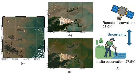
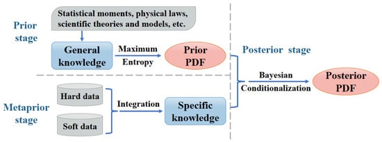
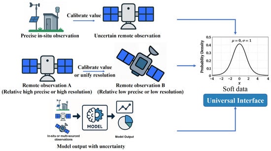
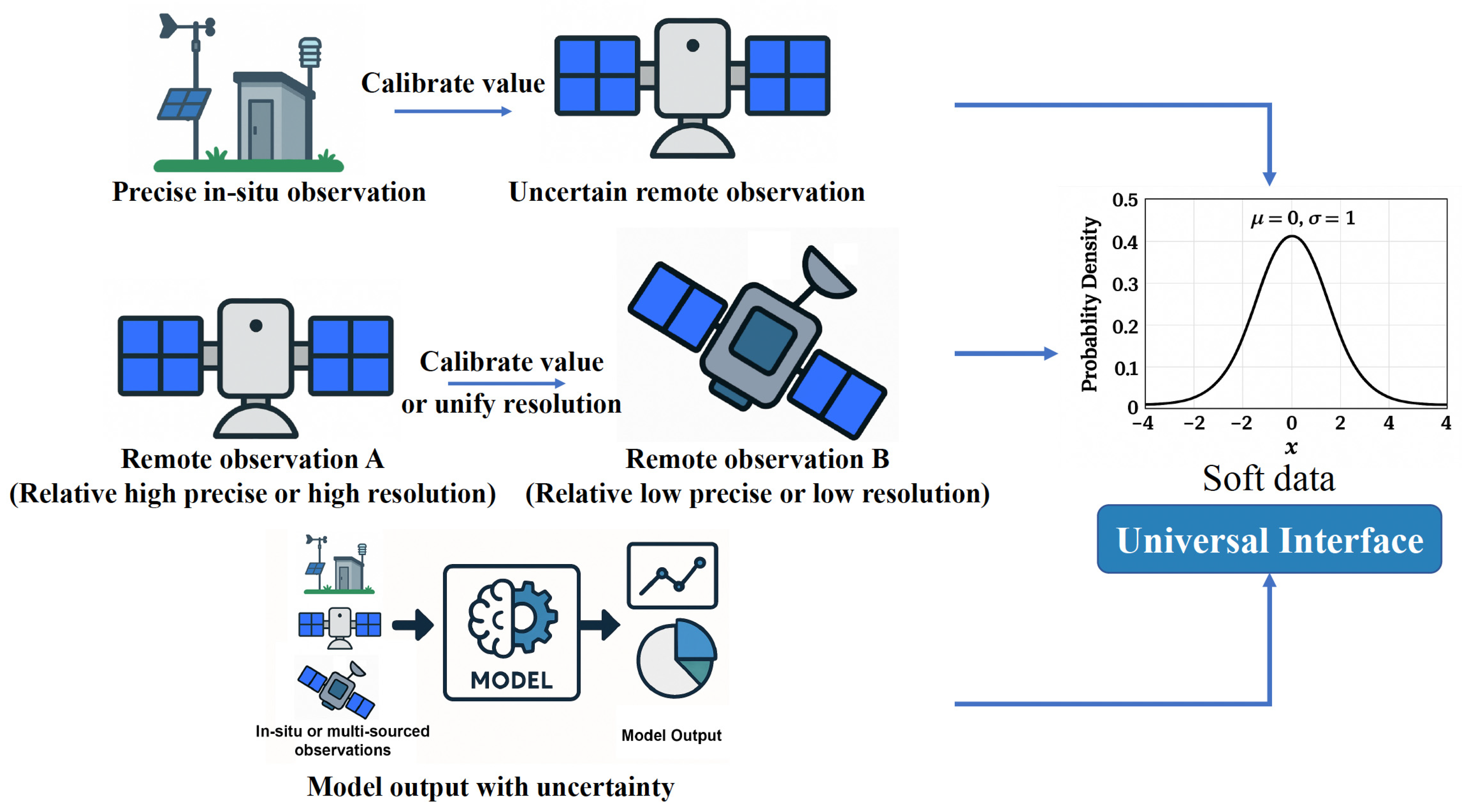
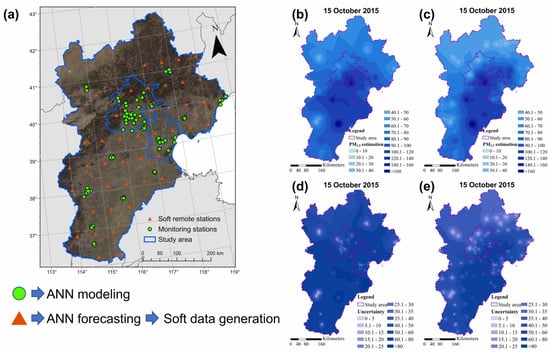
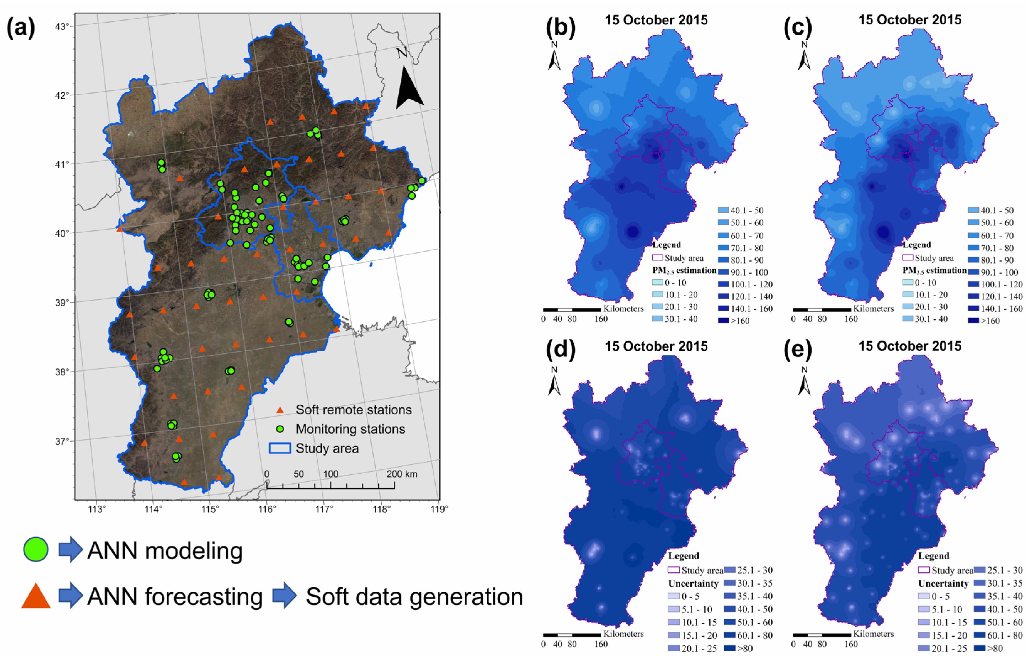
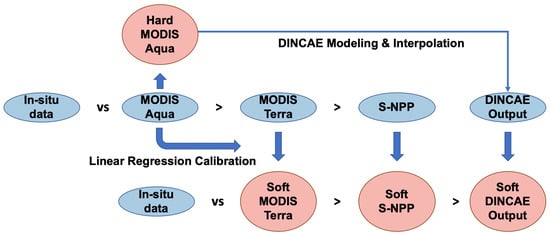
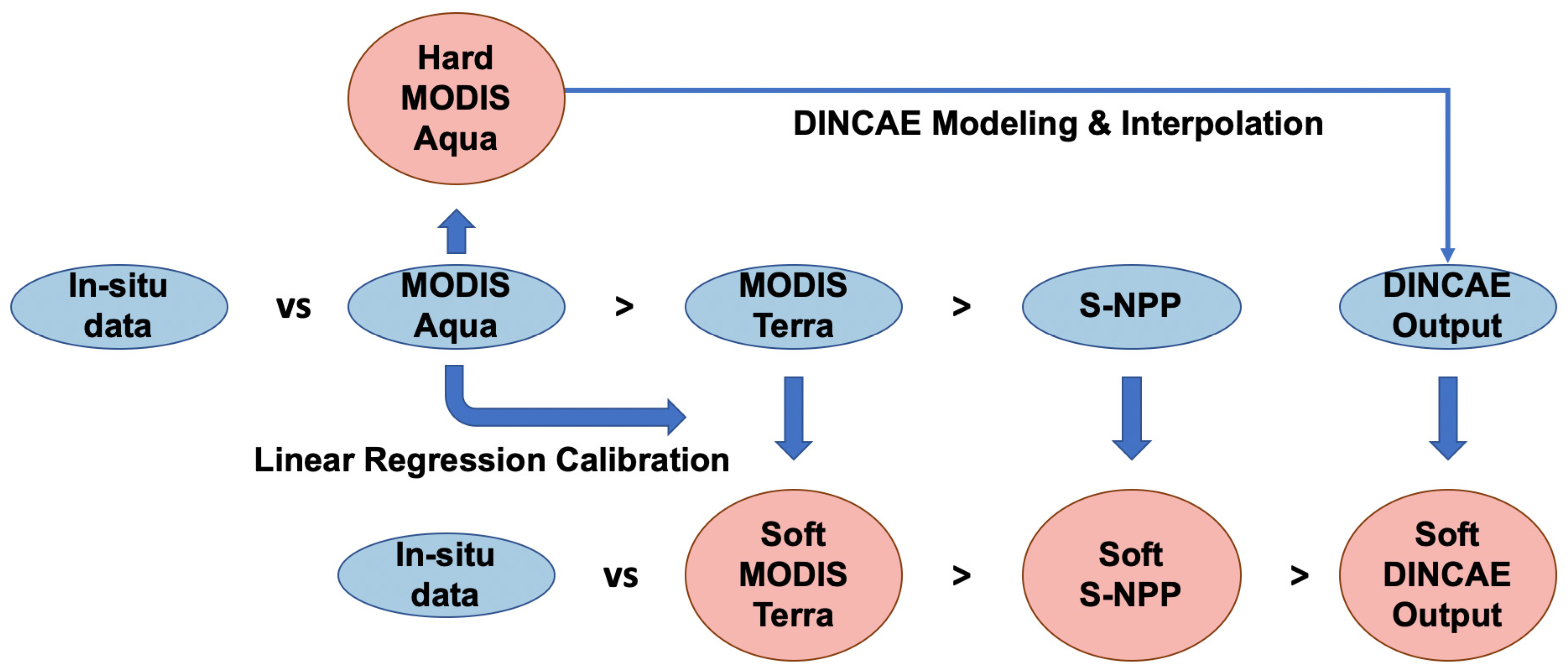

Disclaimer/Publisher’s Note: The statements, opinions and data contained in all publications are solely those of the individual author(s) and contributor(s) and not of MDPI and/or the editor(s). MDPI and/or the editor(s) disclaim responsibility for any injury to people or property resulting from any ideas, methods, instructions or products referred to in the content. |
© 2026 by the author. Licensee MDPI, Basel, Switzerland. This article is an open access article distributed under the terms and conditions of the Creative Commons Attribution (CC BY) license.