Rainforest Monitoring Using Deep Learning and Short Time Series of Sentinel-1 IW Data

Highlights

What are the main findings?

• Short time series of Sentinel-1 SAR and InSAR data trained with a U-Net-like model have shown great potential as a radar-only system for land cover classification in the Amazon rainforest, paving the way for the generation of medium-resolution forest maps with unprecedented temporal resolution.
• Continuous monitoring of the state of the forests faces seasonal challenges, in which radar data can be affected by meteorological conditions and confused with actual changes of land cover classes if not properly addressed.

What are the implications of the main findings?

• Once generated, monthly land cover maps from environmentally critical tropical regions may be used as a supporting tool for a series of applications, such as change detection in the scope of deforestation monitoring.
• The present study highlights the importance of considering temporally stable references and a proper seasonal sampling strategy for the training data over areas with well-defined seasons.

Abstract

The latest advances in remote sensing play a central role in providing Earth observation (EO) data for numerous applications in the scope of reaching environmentally sustainable goals. However, over tropical rainforests, optical imaging is often hindered by extensive cloud coverage, which means that analysis-ready images are mostly restricted to the dry season. In this study, we propose combining radar features extracted from short time series of Sentinel-1 Interferometric Wide Swath (IW) data with a deep learning-based classification scheme to continuously monitor the state of forests. The proposed methodology is based on the joint use of SAR backscatter and interferometric coherences at different temporal baselines to perform pixel-wise classification of land cover classes of interest. However, we show that for a sequence of Sentinel-1 time series, different land cover classes exhibit particular seasonal-dependent variations. Another challenge in performing short-term predictions stems from the fact that ground truths are usually available only on a yearly basis. To address these challenges, we propose a seasonal sampling of the training data, masked by potential deforestation, along with a classification based on a modified U-Net model. The classification results show that overall accuracies above 90% can be achieved throughout the whole year with the proposed method, emerging as a potential tool for mapping rainforests with unprecedented temporal resolution.

1. Introduction

Rainforests are the most biodiverse ecosystems on the planet. Their environmental importance extends to major bio-physical processes, such as regulating the climate, water, and carbon cycles, not only locally but also at a global scale. As the world’s largest rainforest, the Amazon plays a central role in climate change mitigation and is also home to a wide diversity of flora, fauna, and indigenous peoples. However, in recent years, the Brazilian Legal Amazon alone has suffered an estimated mean annual primary forest loss of around one million hectares [1], which threatens the sustainable management of this ecosystem.

In light of the growing awareness towards preservation policies, a series of joint international efforts aiming at the systematic observation of humid forests, such as the United Nations’ Reducing Emissions from Deforestation and Forest Degradation (REDD+) program [2], have been undertaken. In this scenario, remote sensing is unique in providing large-scale coverage and temporal consistency required for these tasks. For the Brazilian Amazon, these data are provided mainly by the Brazilian Amazon Rainforest Monitoring Program by Satellite (PRODES) and the Real-Time Deforestation Detection System (DETER) [3] of the Brazilian National Institute for Space Research (INPE). While PRODES is primarily based on Landsat imagery at medium resolution to compute yearly deforestation statistics, DETER mostly uses China–Brazil Earth Resources Satellite-4 (CBERS-4) and Indian Remote Sensing Satellite (IRS) data to alert potential forest disturbances. In addition to identifying deforestation, qualifying natural resources and tracking land use are of utmost importance for implementing sustainable policies. In this context, the TerraClass project was created in 2010 with the goal of classifying the use of deforested areas based on PRODES data [4], and it is updated every two years. More recently, the MapBiomas project [5] has established itself as one of the main references for understanding land use dynamics in the Amazon forest, and since 2015, it has been producing annual land cover and land use maps from 1985 to the present date.

Currently, most solutions for monitoring landscape changes in such vast areas rely on optical spaceborne data, whose effectiveness is typically restricted to local dry seasons due to persistent cloud cover during the rest of the year. While optical data remain the backbone of forest monitoring, the advent of spaceborne microwave sensors through synthetic aperture radar (SAR) systems offers the invaluable advantage of acquiring images independently of daylight or local atmospheric conditions. The Sentinel-1 mission, comprising two polar-orbit satellites with C-band SAR imaging capabilities, paved the way for consistently monitoring the Earth’s surface by providing openly available medium-resolution data over global landmasses at a 12-day repeat cycle. In particular, Sentinel-1 time series acquired in Interferometric Wide Swath (IW) mode have shown potential for land cover monitoring in the Amazon rainforest. In [6], short time series of SAR backscatter have been used as input features to a Random Forest (RF) classifier along with a temporal decorrelation model [7] in order to better characterize different land cover classes. For longer temporal baselines, the work in [8] used a support vector machine (SVM) classifier and reported little differences when adding short- and long-term coherence statistics from annual time series in comparison to backscatter-only information. The work in [9] investigated the potential of convolutional neural networks (CNNs) for land cover classification with a Sentinel-1 time series of 24 days, reporting a higher accuracy than a shallow learner while requiring less processing. However, there is still a research gap regarding the systematic mapping of the rainforest and the characterization of different land cover classes amid different seasons and study sites in such a complex environment as the Amazon biome.

In the pursuit of developing a year-round rainforest monitoring system, we first build on the works in [6,7,9] to investigate the joint use of SAR backscatter and the evolution in time of the temporal decorrelation between pairs of interferometric acquisitions to discriminate different types of land cover. We then show that on a large scale and over a longer observation period, these radar data might fluctuate not only because of noise but also due to seasonal components, increasing interclass confusion and affecting classification performance. In the case of SAR backscatter, speckle effects and the instability of the signal due to changes in atmospheric conditions and soil moisture [10] constitute major challenges for forest monitoring. Since dense forests expose less of the soil, they are less impacted by these instabilities. However, as most non-forest classes are more susceptible to such variations, they occasionally look similar to forest classes [11]. The complimentary use of interferometric coherences can help to distinguish some of these classes to a certain extent. While forests typically exhibit low coherence even at short temporal baselines when compared to sparse vegetation and grasslands, changes in precipitation might decrease temporal coherence and make the interpretation ambiguous [12].

In this paper, we propose relying on a sequence of Sentinel-1 interferometric time series with high temporal resolution to reduce noise in the data and derive reliable classification maps at frequent observation intervals. In order to deal with the challenges of spatial and temporal noise from SAR images and given the large amount of available Sentinel-1 IW data, we propose exploiting deep learning solutions based on CNNs, aiming at learning complex functions in high-dimensional data with the minimum computational effort possible. To this end, we initially process Sentinel-1 IW short time series covering Rondonia, a region of the Amazon rainforest with an extensive history of deforestation. The term short time series is defined in this paper to highlight the limited time span of 24 days (only three consecutive acquisitions, for a revisit time of 12 days) chosen for the image stacks, which is significantly shorter with respect to most multi-temporal InSAR applications. Then, we investigate different sampling and filtering strategies to achieve a robust forest mapping framework at regular intervals based on a U-Net-like architecture [13]. The results are then validated with independent external references and demonstrate the potential of our radar-based method to systematically generate land cover maps over the Amazon.

The remainder of this paper is structured as follows: Section 2 describes the study sites and both the Sentinel-1 data and the references used in this paper, as well as the proposed forest monitoring system, including the processing and analysis of the time series and the deep learning framework. The experimental results are presented in Section 3. In Section 4, the potential and challenges of the proposed approach are discussed in greater detail. Finally, Section 5 summarizes the contributions of this paper and sheds light on possible future research.

2. Materials and Methods

2.1. Study Sites

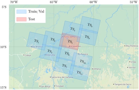
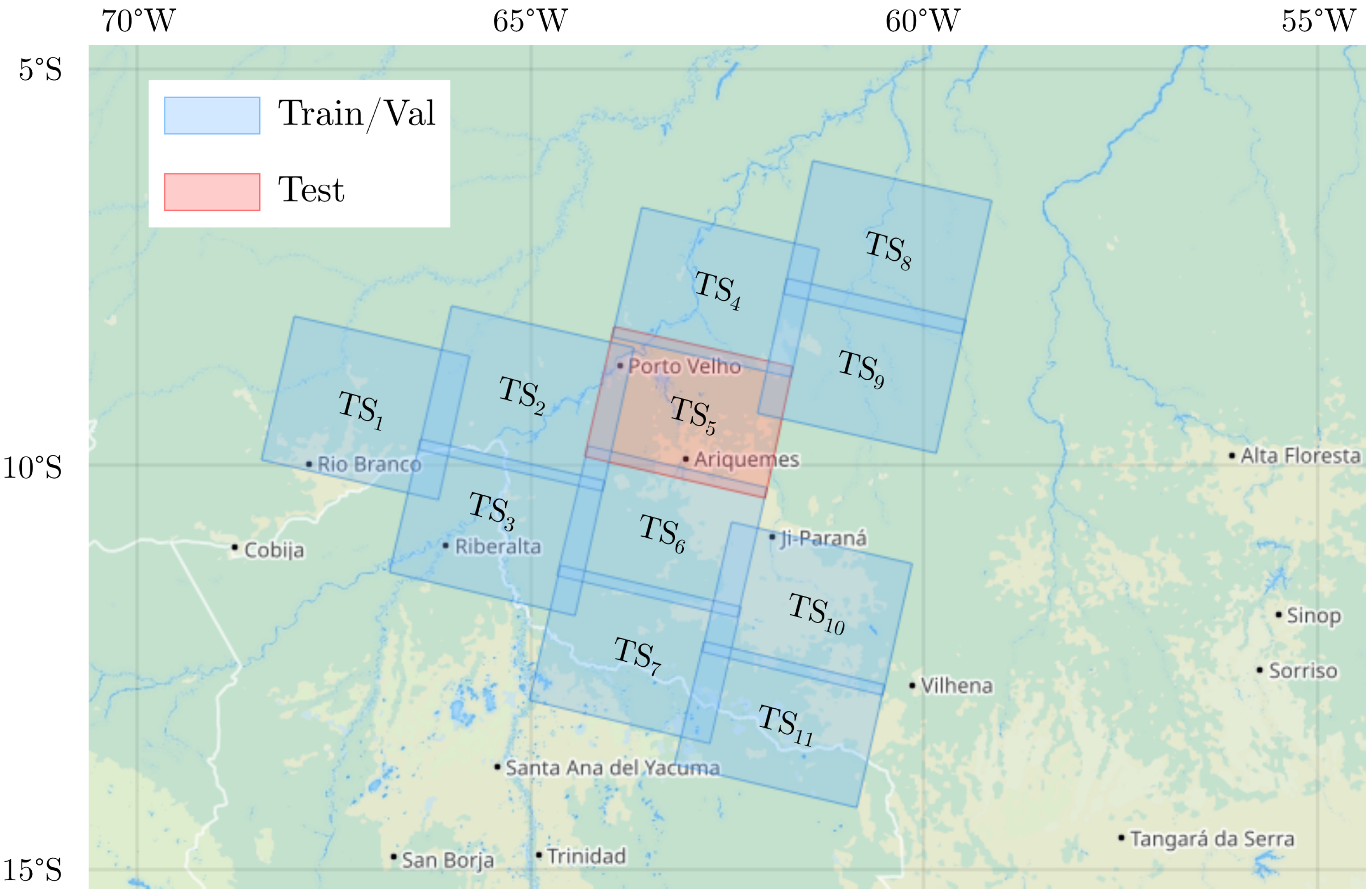
The study area is located around the Brazilian state of Rondonia, a region predominantly covered by forests despite hosting one of the most diverse landscapes within the Amazon biome, with the presence of grasslands, croplands, river branches, and urban settlements. Moreover, this is historically one of the most deforested places in the Amazon basin, thus being the target of a series of studies concerning landscape changes [14,15,16,17]. The study sites cover an area of approximately 440,000 km² and are delimited by Sentinel-1 acquisitions, as can be seen in the footprints of Figure 1.

Figure 1. Study sites in the Amazon forest. The 11 footprints were considered for mapping the rainforest by processing sequences of Sentinel-1 interferometric short time series (TS), divided into two sets: training and validation (in blue) and test (in red).

2.2. Sentinel-1 Data

The Sentinel-1 mission comprises two satellites, originally Sentinel-1A and Sentinel-1B (the latter substituted by Sentinel-1C, which has been launched in December 2024), in a near-polar sun-synchronous orbit with a 180° orbital phasing difference. Each satellite has a repeat cycle of 12 days with 175 orbits per cycle. With the full constellation operational, most global landmasses can be imaged every 12 days, while Europe and a few selected areas are imaged every 6 days with information from both satellites.

Over the last years, Sentinel-1 Interferometric Wide Swath (IW) products have been widely used for a series of land monitoring applications thanks to their free and open data policy, wide spatial coverage, and high temporal resolution. In this work, we consider focused Single-Look-Complex (SLC) images provided at dual-polarization VV + VH with a nominal spatial resolution of 22 × 3.1 m in azimuth and slant-range at the central sub-swath, respectively, and an independent pixel spacing of 14.1 × 3.7 m in azimuth and ground range, respectively. In total, we processed 140 short time series of Sentinel-1 IW data throughout 2017 to monitor an environmental critical area in the Amazon rainforest. In each time series, the target scene is observed for a temporal span of only 24 days, based on three consecutive repeat-pass acquisitions with a revisit time of 12 days. The full list of acquisitions is detailed in Appendix A.

2.3. Reference Data

2.3.1. FROM-GLC Thematic Maps

The Finer Resolution Observation and Monitoring of Global Land Cover (FROM-GLC) was the first 30 m global land cover product [18], based on Landsat imagery. This concept was further developed for the generation of the 2015 FROM-GLC thematic map based on an all-season sample set, which was updated by transferring the learning from the 2015 dataset into Sentinel-2 images obtained in 2017, resulting in a 10 m map with more spatial details and less cloud impact even in critical regions [19].

The 2017 FROM-GLC map is divided into 10 land cover classes: cropland, forest, grassland, shrub, wetland, water, tundra, impervious, bareland, and snow/ice. It should be noted that in this scheme, the concept of land use is avoided whenever possible (e.g., harvested agricultural lands are classified as bareland with respect to their land cover function) [18]. Moreover, most of the possible land cover classes are not well represented on the study sites, which are areas predominantly covered by forest and pasture fields (here regarded as grassland).

2.3.2. PRODES Deforestation Rates

Since 1988, the Brazilian Amazon Rainforest Monitoring Program by Satellite (PRODES) system [3] is responsible for estimating primary forest losses using Earth observation satellite images for the entire extension of the Brazilian Legal Amazon (BLA), an area totaling around 5 million km². PRODES uses satellite images from the Landsat class (20 to 30 m spatial resolution and a revisit time of 16 days), preferably within the dry season of each scene. In areas with successive cloud cover, Sentinel-2 and China–Brazil Earth Resources Satellite-4 (CBERS-4) data are also used complementarily in order to minimize the lack of observations.

In the PRODES methodology, deforestation is defined through photointerpretation of the images by trained specialists who identify patterns of change in forest cover according to tone, color, shape, texture, and context [20]. In order to generate an annualized rate of deforestation in a scene, the maps are projected onto a common reference date, 31 July, considering that for most of the images, the dry season occurs from June to September.

2.3.3. MapBiomas

The MapBiomas project was launched in 2015 with the goal of better describing the yearly dynamics of land use and land cover (LCLU) over all Brazilian biomes. Dividing the territory into biomes helps define—and thus classify—different landscape patterns across the country [5]. Analogously to PRODES, the MapBiomas maps are based on the Landsat series archive, from 1985 to the present day. At the first hierarchical level, five classes can be defined: forest, herbaceous and shruby vegetation, farming, non-vegetated area, and water. Level 2 has 20 classes based on those from the first categorical level. Agriculture is the only class with further subdivisions, amounting to 27 land cover classes in total.

Aside from yearly LCLU maps, MapBiomas also publishes transition maps to describe landscape changes of interest such as: transitions from non-vegetated areas to forest cover, areas with increases or decreases in water surface, and deforestation. Similarly to the generation of LCLU maps, spatial filtering is used to eliminate single pixels or small pixel clusters in the borders of different classes derived from the creation of transition maps.

2.4. Problem Statement

In this paper, we use a deep learning approach to leverage short-term information from Sentinel-1 IW SLC temporal series for characterizing the fast-changing state of the Amazon forest. To this end, we propose using time series of only 24 days (i.e., three acquisitions for a repeat cycle of 12 days with a single operating satellite, which is globally available for landmasses) to generate medium-resolution land cover maps over environmentally critical areas. Within the scope of this work, we consider as SAR backscatter measurement the gamma nought coefficient ${\gamma }^0$—whose normalization is performed to an area perpendicular to the radar’s line of sight—to compensate for the acquisition geometry across the mainly flat terrain of the Amazon forest.

Next, we exploit the concept of interferometric SAR (InSAR), which employs two or more complex-valued SAR images to extract additional information about the scene. In the scope of this work, we consider repeat-pass interferometry, in which the same area is imaged with a certain temporal baseline separation (e.g., 12 and 24 days). The interferometric coherence constitutes the main metric in SAR interferometry by providing a measurement of the interferometric phase quality (i.e., the noise level in the interferogram). The coherence is defined as the normalized complex correlation between a pair of coregistered SAR images, $S_1$ and $S_2$, according to

$$\rho ={\displaystyle \frac{E\left[S_1{S}_2^{*}\right]}{\sqrt{{E\left[\right|S_1|}^2\left]E\right[|S_2{|}^2]}}},$$

(1)

where $E[·]$ is the mathematical expectation and * denotes the complex conjugate operator. Following common practice in the literature and assuming stationarity and ergodicity of the processes in (1), the interferometric coherence is given by averaging the sample coherence magnitude computation which represents its maximum likelihood estimate:

$$\widehat{\rho }={\displaystyle \frac{\left|{\sum }_{i=1}^L\left(S_{1_i}{S}_{2_i}^{*}\right)\right|}{\sqrt{{\sum }_{i=1}^L{\left|S_{1_i}\right|}^2·{\sum }_{i=1}^L{\left|S_{2_i}\right|}^2}}},$$

(2)

where L is the number of samples in the window.

Conceptually, the interferometric coherence can also be expressed as a product of different decorrelation sources [21]:

$${\rho }_{\mathrm{tot}}={\rho }_{\mathrm{SNR}}·{\rho }_{\mathrm{quant}}·{\rho }_{\mathrm{amb}}·{\rho }_{\mathrm{az}}·{\rho }_{\mathrm{rg}}·{\rho }_{\mathrm{vol}}·{\rho }_{\mathrm{temp}},$$

(3)

where ${\rho }_{\mathrm{SNR}}$ represents the contributions due to limited signal-to-noise ratio (SNR), ${\rho }_{\mathrm{quant}}$ describes quantization noise, ${\rho }_{\mathrm{amb}}$ represents the ambiguities, ${\rho }_{\mathrm{az}}$ is related to the relative shift of the Doppler spectra, ${\rho }_{\mathrm{rg}}$ describes baseline decorrelation, ${\rho }_{\mathrm{vol}}$ is associated with volume decorrelation, and ${\rho }_{\mathrm{temp}}$ is related to temporal decorrelation. In the case of Sentinel-1, the orbits are stable with small baselines, leading to ${\rho }_{\mathrm{rg}}$ and ${\rho }_{\mathrm{vol}}$ values close to unity. Although some of the other decorrelation sources are non-negligible, in particular ${\rho }_{\mathrm{SNR}}$, in this work, we focus on the role of ${\rho }_{\mathrm{temp}}$ by leveraging how land cover classes of interest decorrelate at different temporal baselines.

2.5. Processing of Sentinel-1 InSAR Short Time Series

The processing of the Sentinel-1 data is performed using the TanDEM-X interferometric processor (TAXI) [22] developed at the DLR Microwaves and Radar Institute and follows the practices of [6,7,9,23] for processing Sentinel-1 TOPS data. In this work, each time series consisting of three IW SLC data acquired 12 days apart is processed as follows: First, the image stack is coregistered with respect to a common master, using precise orbit information and an external digital elevation model (DEM). For the scope of this work, the master image is defined as the one closest to the central date of the stack. Moreover, it should be noted that all the following processing steps are performed separately for the VV and VH polarizations.

Then, we can perform the radiometric calibration of the images to ${\widehat{\gamma }}^0$ according to

$${\widehat{\gamma }}^0=K·D{N}^2·tan\left({\theta }_i\right),$$

(4)

where K is the SAR calibration constant of the Sentinel-1 annotated files, the digital number ($DN$) denotes the focused SAR amplitude, and ${\theta }_i$ is the local incidence angle estimated from Shuttle Radar Topography Mission (SRTM) data. For this backscatter measurement, a simple boxcar filter of 1 sample in azimuth and 5 samples in range is used as spatial multi-looking, providing some speckle filtering while still preserving the product’s resolution. Within the framework of this study, we consider that a single land cover class should be assigned per pixel based on the features derived from the time series. Moreover, we assume stationarity of the scene and that the land cover classes do not change within the time span of 24 days, so that any pixel-wise variations are assumed to be noise. Therefore, the resulting backscatter stack is averaged along the temporal dimension into a single image ${\widehat{\gamma }}_{\mathrm{avg}}^0$, acting as a temporal despeckling filter and reducing the required number of feature channels.

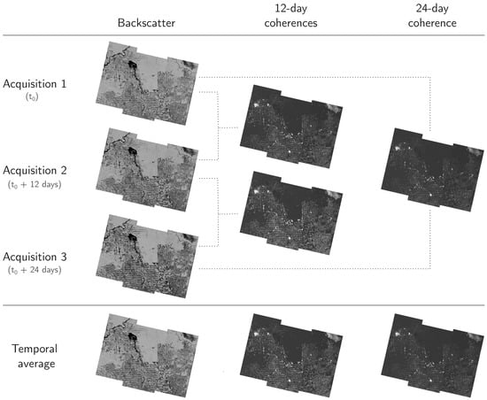
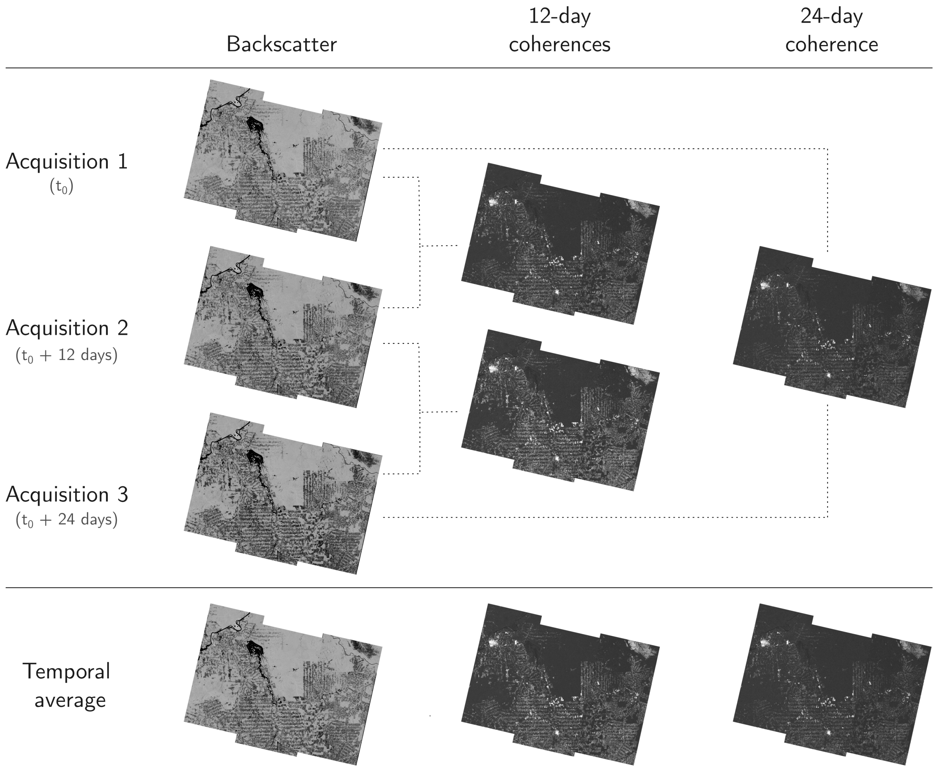
Regarding the estimation of the interferometric coherences, a boxcar of size 5 × 19 samples (in azimuth × range, respectively) has been used instead. This kernel size results in images with a resolution cell of approximately 100 m, which was deemed a good compromise between the loss in spatial resolution information and the mitigation of the bias over lower-coherence areas as described in [24]. Therefore, the resulting interferometric products of interest are two coherence images ${\widehat{\rho }}_{12}$ with a temporal baseline of 12 days (computed between the central date acquisition and both the first and last) and one interferometric coherence image ${\widehat{\rho }}_{24}$ with a 24-day separation. Following the method adopted for the backscatter, we assume stationarity of the scene and the 12-day interferometric coherences are averaged in time so each feature is represented by a single image. The SAR and InSAR features considered within a single time series are illustrated in Figure 2. Finally, after geocoding to a common grid, the images are posted at 20 m × 20 m in order to exploit the full resolution of the backscatter measurements.

Figure 2. Example of features of interest generated during the Sentinel-1 time series processing. Within the framework of this work, the gamma naught backscatter and the 12-day interferometric coherences are averaged in time.

2.5.1. Long-Term Data Analysis: Seasonalities

In the scope of achieving a robust dataset based on short time series for monitoring the state of the rainforest, we now analyze the processed Sentinel-1 IW acquisitions shown in Figure 1. For each study site, between 10 and 13 time series from 2017, each comprising 24 days, were processed at dual-polarization VV + VH with a pixel spacing of 20 m (with nominal feature spatial resolution ranging from 20 m to 100 m). This represents a unique data collection to further understand the highly complex natural and anthropogenic dynamics that dictate the state of the Amazon biome throughout the seasons.

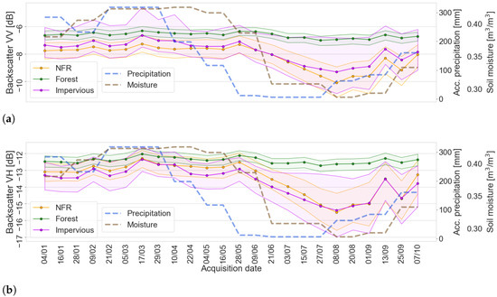
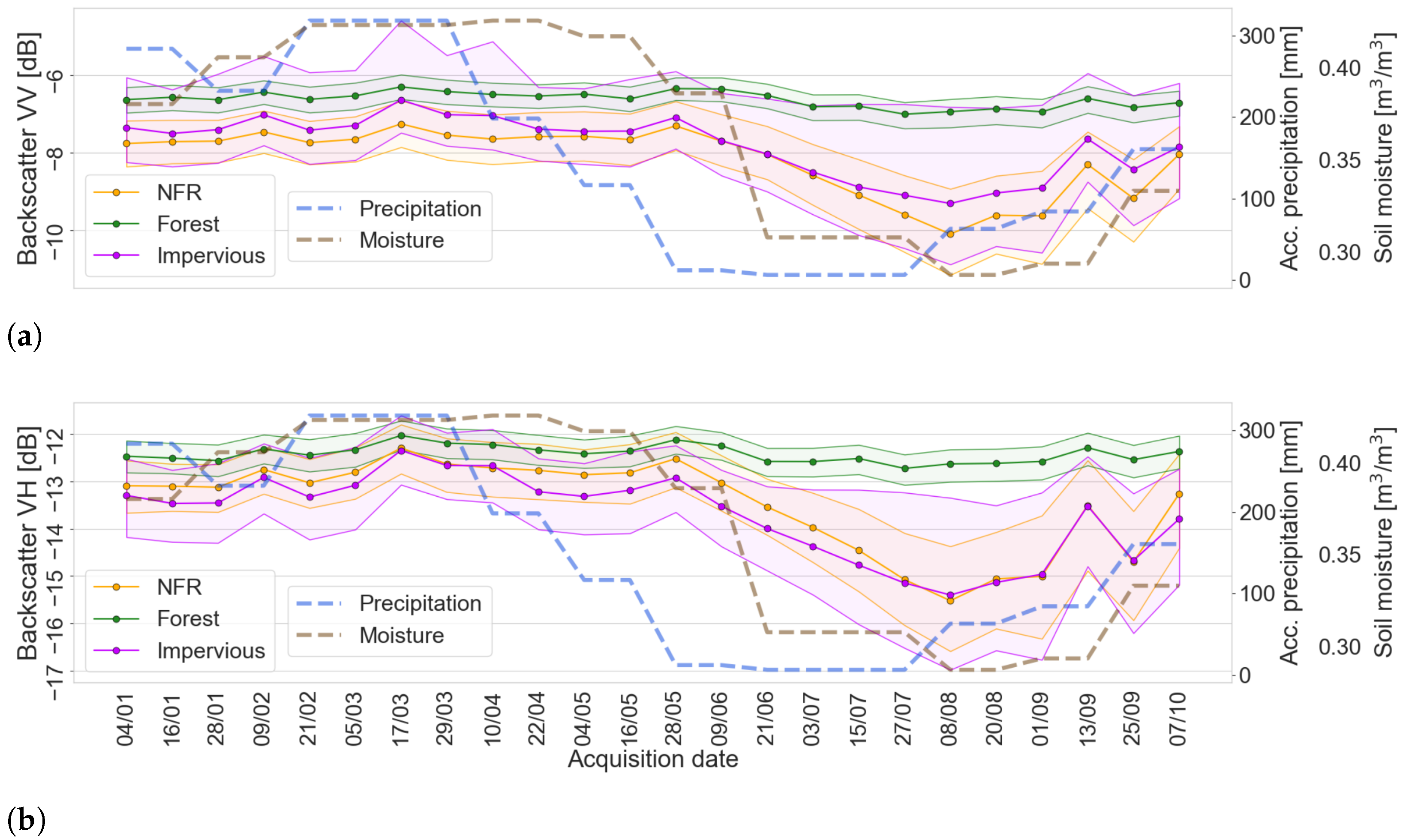
Thus, we also investigate the impact of auxiliary data over these observations (e.g., precipitation statistics, soil moisture estimation, date of image acquisition). Figure 3a and Figure 3b show the evolution in time of the backscatter measurement ${\widehat{\gamma }}^0$ in VV and VH polarizations, respectively, for the test footprint of Figure 1 when considering three classes of the FROM-GLC reference: forest, impervious, and non-forest region (NFR)—the latter being a grouping of all the remaining classes except for water, mostly composed of grasslands and pastures. The figure shows the spread of backscatter VV (centered around its median and ranging from the 25th to the 75th percentile) in the Rondonia test site for the different land cover classes. It can be seen that while the forest areas remain relatively stable, the remaining classes suffer a seasonal attenuation—which is more pronounced between the months of June and September, associated with the dry season in this region. This pattern is also verified in VH polarization, and can be further validated by comparing the radar data with local precipitation (shown as blue dashed lines) and soil moisture (in brown) estimations from Climate Hazards Group InfraRed Precipitation with Station (CHIRPS) data [25,26]. In this case, the separability of forest, impervious, and NFR is higher when precipitation and soil moisture levels are lower.

Figure 3. Median spread of the estimated backscatter ${\widehat{\gamma }}^0$ in (a) VV and (b) VH between January and October 2017 in the region of Rondonia for three land cover classes: NFR, forest, and impervious. Strong seasonal variations are observed between June and September, during the dry season, when the classes are more easily discernible following a decrease in precipitation and soil moisture trends.

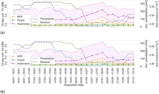
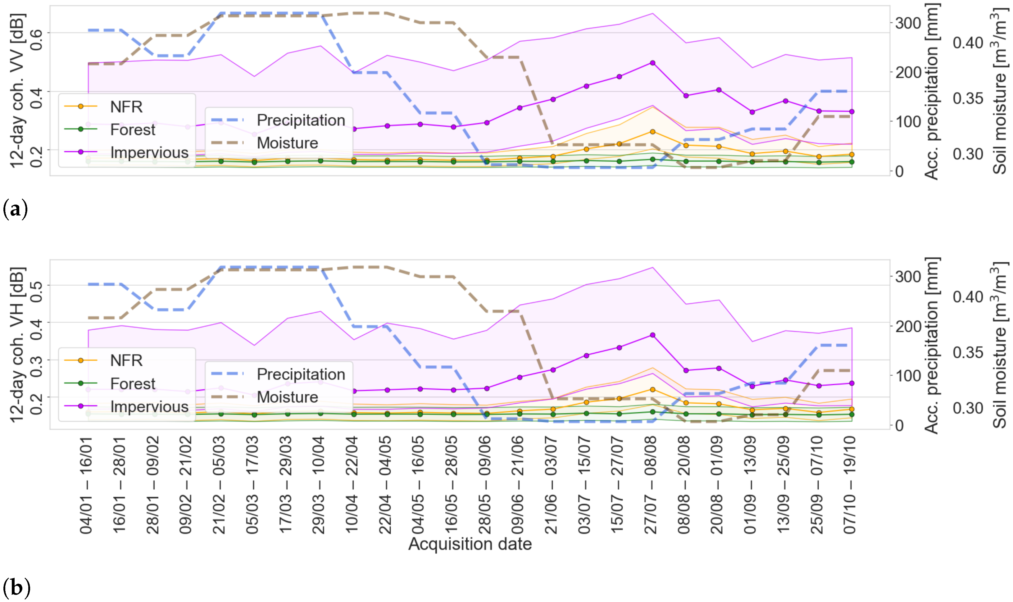
Analogously, Figure 4a,b shows the behavior of 12-day interferometric coherences in VV and VH throughout the year. Despite showing a smaller dynamic range and an overall greater class overlap during the entire observation period, the coherences provide complementary information to the backscatter measurements, as the three classes of interest can be better separated during the drier months, between June and September. A similar behavior can be observed at larger temporal baselines (i.e., 24-day coherences), which exhibit greater separability of the impervious class at the expense of more ambiguities between forest and NFR.

Figure 4. Median spread of the estimated 12-day coherences ${\widehat{\rho }}_{12}$ in (a) VV and (b) VH along 2017. It can be seen that there is a large overlap between NFR and forest for most of the year, but the classes are even more separable than for backscatter during the dry season.

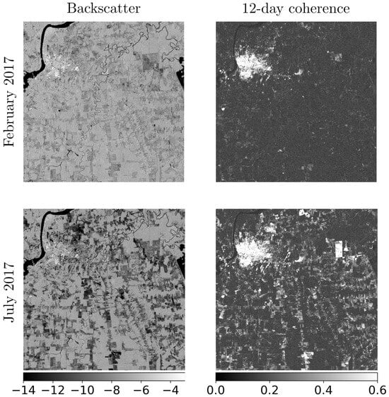
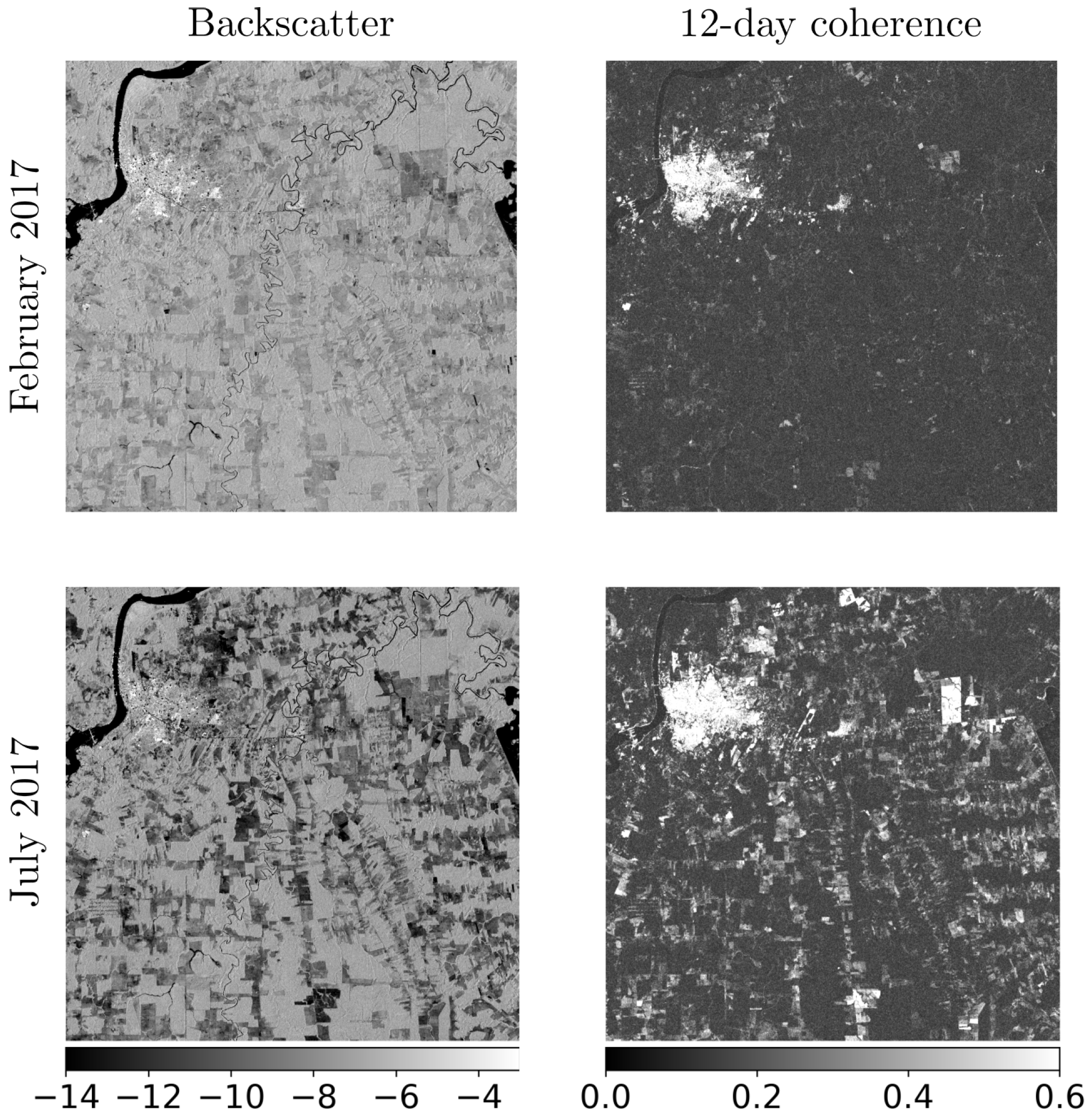
The aforementioned seasonal variations represent an additional challenge to the continuous monitoring of the Amazon forest, as they can be confused with actual changes in the land cover classes. Thus, this study includes discerning actual changes on the ground that would indicate the change of a class over time (deforestation, vegetation regrowth, fluvial drought, etc.) from intraclass effects (variations on the SAR backscatter of grasslands depending on the humidity level and on the interferometric coherence of fields according to cropping cycles, for instance). Figure 5 illustrates how impactful seasonal effects can be on the SAR backscatter and 12-day interferometric coherences. Although no significant land cover changes are expected between February and July 2017 around the city of Porto Velho, the first acquisition exhibits a higher ambiguity between different land cover classes.

Figure 5. Seasonal effects on both backscatter (in dB) and 12-day coherences in VV. Even though no significant land cover changes are expected between the acquisitions, the input features are significantly affected by temporal changes (i.e., seasonalities).

2.6. Proposed Deep Learning-Based Land Cover Classification Scheme

The U-Net [13] has become one of the most widespread image segmentation models in remote sensing thanks to its flexibility and ability to deal with smaller datasets—which is the case for most SAR-oriented deep learning problems. The U-Net architecture is composed of two parts. The encoder or contracting path consists of a series of downsampling convolutional levels to extract high-level semantic features and contextual information as the network goes deeper. However, this process results in a progressive loss of spatial resolution and localization of extracted features. The second part of the network consists of the decoder or expansive path, where upsampling levels based on transposed convolutions are used to gradually recover the image’s resolution while condensing the feature dimension. The breakthrough of the U-Net lies in its skip connections, in which the outputs of each convolutional level of the encoder are propagated to the corresponding stage of the decoder. This design enables the combination of high-resolution context information with high-level representations for accurate localization of the extracted features.

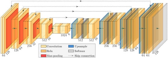
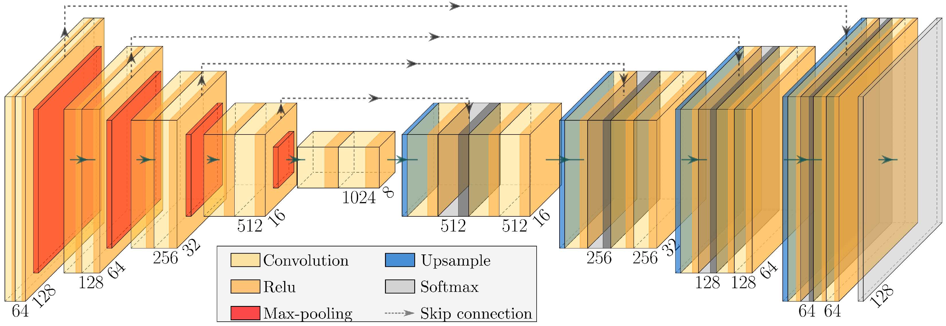
Within the scope of our problem, we propose implementing a U-Net-like model tailored to our problem, as shown in Figure 6. First, as a common practice in the remote sensing literature, the input image patches are padded with zeros before convolutions to avoid affecting their size (i.e., original resolution) along the network. Moreover, through hyperparameter tuning, we set the number of convolutional levels to five, reaching 1024 feature maps in the deepest level for a total of 31,046,020 learnable parameters, in accordance with the large dataset considered in this work. As the loss function, we use the categorical cross-entropy between one-hot encoded labels and the predicted probability distributions from a softmax output layer. Finally, batch normalization is performed at every convolutional level as the regularization method, allowing for a faster and more stable training phase.

Figure 6. Proposed U-Net-like model implementation with five convolutional levels.

2.6.1. Baseline Database Preparation

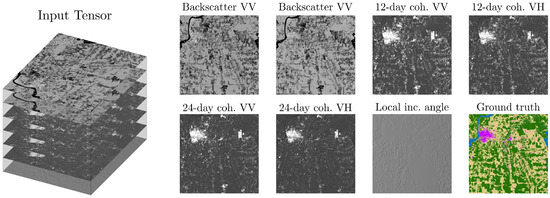
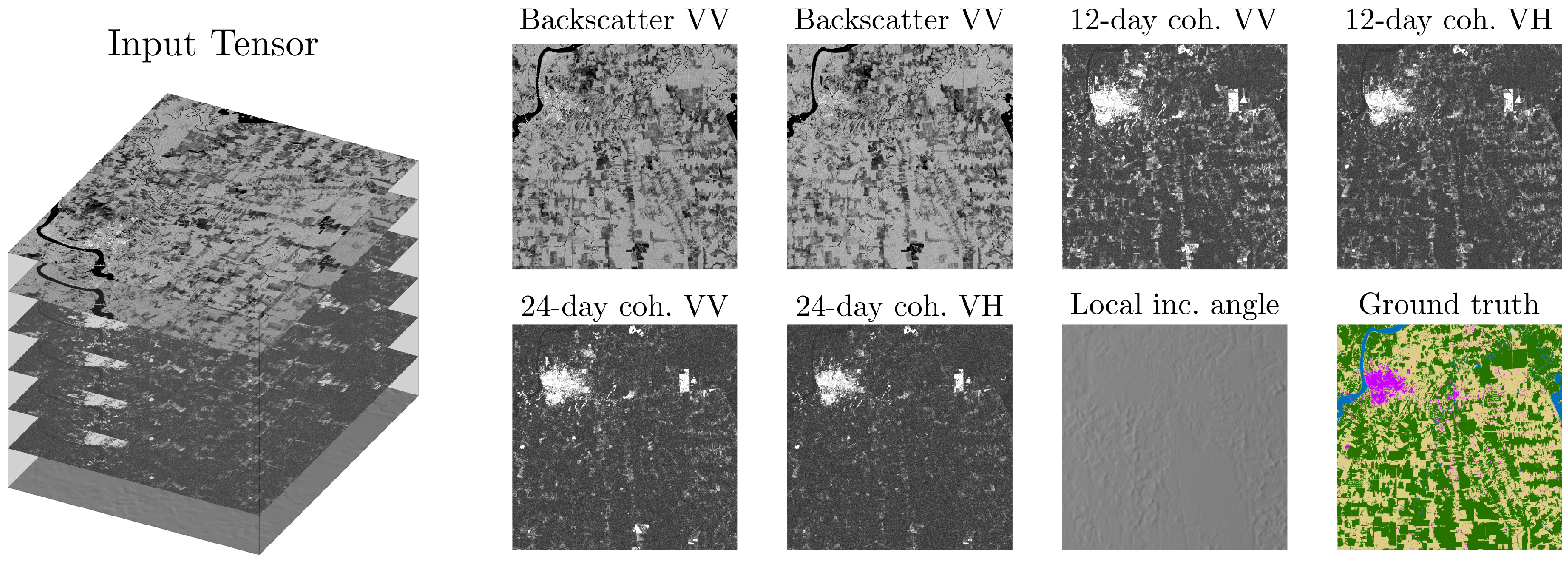
The input data for the CNN are composed of N image patches in the shape of a $P\times P\times C$ array, where P is the patch size (in pixels) and C is the number of channels in the network (i.e., input features). The input tensor in this work is then shown in Figure 7, which considers the average SAR backscatter and interferometric coherences with 12- and 24-day baselines, at both VV and VH polarizations. Moreover, the local incidence angle estimated from SRTM data is included as a geometrical feature.

Figure 7. Baseline input feature setting. In total, seven features from SAR, InSAR, and geometrical properties are considered in this work and trained with respect to the ground truth, here adapted from the FROM-GLC or MapBiomas thematic maps as further detailed in Section 2.6.1. Impervious areas are shown in magenta, water in blue, non-forest regions (NFR) in yellow-beige and forest in green.

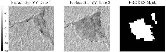
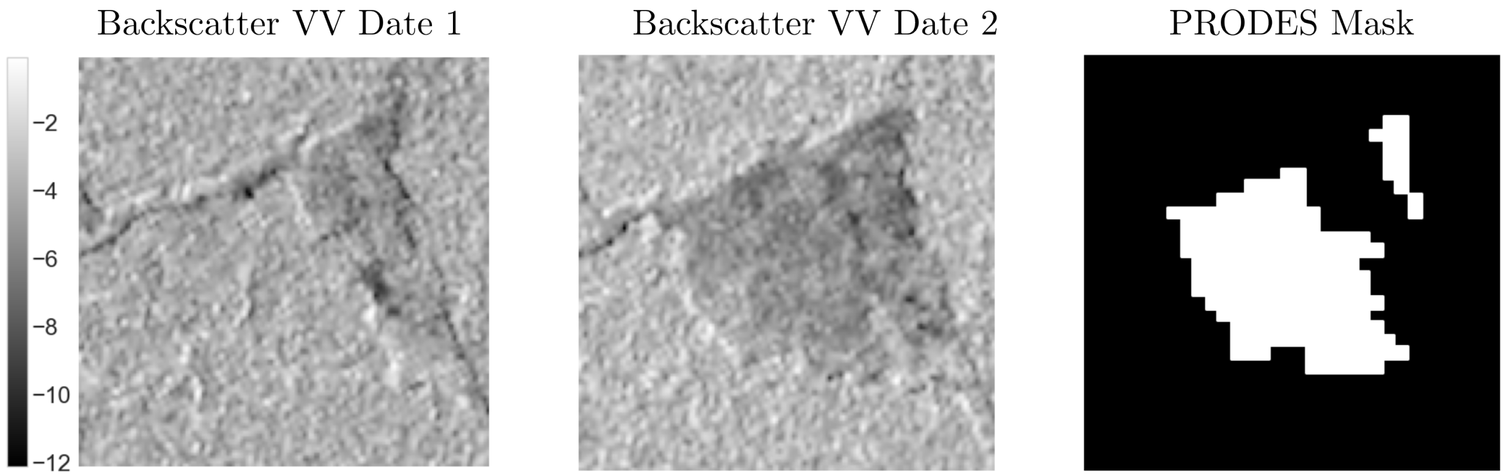
We initially focus on the single generation of a land cover map at 20 m pixel spacing. For this approach, we consider one time series for each of the 11 Sentinel-1 footprints shown in Figure 1. Table 1 shows the relative orbit, acquisition dates, and data splitting strategy of each time series. The period of the year has been defined as towards the end of the wet season, when deforestation may occur but optical images are still severely hindered by cloud cover. Moreover, since the reference data are generated annually and the forest dynamics rapidly change due to both natural and anthropogenic activities, a PRODES deforestation mask is applied for the year under analysis with the goal of achieving a more robust and consistent ground truth. Figure 8 shows an example of backscatter data (VV polarization) acquired in July 2017 and 2018, respectively. In this case, the main differences between the input data are caused by a change in land cover, i.e., deforestation, and these samples are excluded from training. Finally, it should be noted that by applying the aforementioned mask, we expect that areas of active deforestation can be sources of confusion for individual classification maps, which are not trained to predict changing pixels.

Table 1. Description of the 11 time series (TS) considered for the baseline dataset according to their relative orbits, as well as their splitting as test or training and validation sets.

	Rel. Orbit	Time Series			Data Split
		Date 1	Date 2	Date 3
TS1	054	08.04.17	20.04.17	02.05.17	Train/Val
TS2	156	09.05.17	21.05.17	02.06.17	Train/Val
TS3					Train/Val
TS4	083	10.04.17	22.04.17	04.05.17	Train/Val
TS5					Test
TS6					Train/Val
TS7					Train/Val
TS8	010	17.04.17	29.04.17	11.05.17	Train/Val
TS9					Train/Val
TS10					Train/Val
TS11					Train/Val

Figure 8. Input data masking according to a 2017–2018 deforestation map (right) from the Brazilian Amazon Rainforest Monitoring Program by Satellite (PRODES) system, where white pixels indicate forest loss. The changes seen between backscatter (in dB) from July 2017 (left) and July 2018 (center) are associated with land cover changes and are excluded from training.

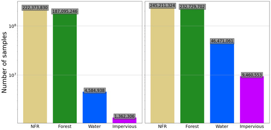
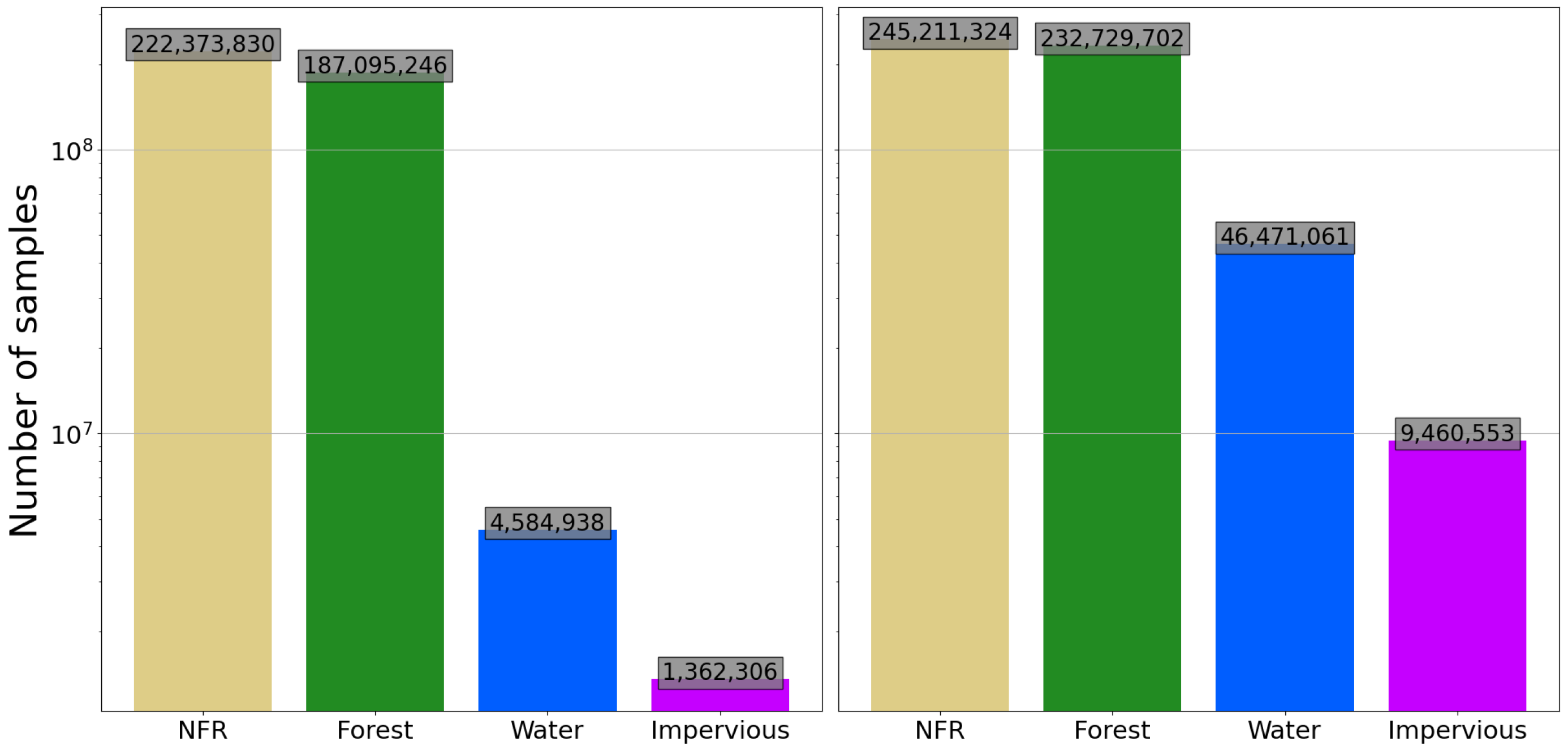
Despite the high availability of training data, the number of samples per class tends to be highly imbalanced in the study sites, with a significant predominance of forest over other land cover: 687,865,895 samples in comparison to 238,092,249 samples of all the remaining land cover classes combined. Since this can lead to prediction biases in machine learning tasks, we propose two dataset balancing procedures. First, we limit the number of classes of interest to four: forest, water, impervious, and non-forest region (NFR). The latter groups land cover classes such as pastures, grasslands, and bareland, being a potential indicator of deforestation over time.

Thus, we first remove excess patches of forest and NFR by following the downsampling rules in Table 2. However, as it can be seen for the FROM-GLC reference in Figure 9 on the left, the dataset remains strongly underrepresented for the classes of water and impervious. Then, we oversample the minority classes of water and impervious by using a sliding window with a stride of 32 pixels for patch extraction over areas where they are properly represented, which we have defined as at least 20% of the total pixels in a patch. This is particularly challenging when considering image patches for training, since augmenting the minority classes usually increases the number of the dominant classes as well (e.g., river and urban settlements are typically surrounded by forests or farming activities). The resulting dataset has a difference of approximately one order of magnitude between forest and impervious (the least-represented class), which was deemed acceptable for the land cover classification problem.

Table 2. Set of rules implemented to balance the training database of Rondonia, originally composed mostly of the forest class ($c_{for}$) and underrepresented in terms of water ($c_{wat}$) and impervious surfaces ($c_{imp}$). For each rule, a fraction of image patches is removed from the database.

Downsampling [%]	Rules
99	$c_{for}==100\%$.
95	$98\%\le c_{for}<100\%$
90	$95\%\le c_{for}<98\%$
85	$88\%\le c_{for}<95\%,c_{wat}<5\%,c_{imp}<5\%$
30	$80\%\le c_{for}<88\%,c_{wat}<8\%,c_{imp}<5\%$
5	$70\%\le c_{for}<80\%,c_{wat}<8\%,c_{imp}<5\%$

Figure 9. Simplified sample distribution after land cover class grouping (left). Given the imbalance of the resulting dataset toward non-forest regions (NFRs) and forest, the minority classes of impervious and water are augmented (right) by extracting patches with a sliding window four times smaller than the patch size in areas where these are well represented.

2.6.2. Seasonal Datasets

Next, we investigate how the baseline database approach of Section 2.6.1 can be used to generate accurate land cover maps at short notice (i.e., every 24 days of Sentinel-1 acquisitions) for continuous monitoring purposes. To this end, we perform a series of tests along an entire year of acquisitions to analyze the impact of seasonalities on the prediction accuracy of the land cover classes of interest, following the findings in Section 2.5.1.

To this end, the methodology adopted for the generation of the training database in Section 2.6.1 is extended to four different seasonal sampling strategies to test the generalization capabilities of the model. First, since the time series shown in Table 1 fall within a period of high precipitation rates, these are chosen to represent the wet season. Analogously, the time series highlighted in red for each footprint in Table A1, Table A2, Table A3 and Table A4 have been chosen to represent dry season data. The third dataset was built with all the acquisitions shown in Appendix A, covering almost a year of acquisitions for all the 11 footprints. Then, a final solution based on the joint use of the first two datasets has been proposed to evaluate a compromise between the required amount of training data and proper seasonal representation.

2.6.3. Training, Validation, and Test Strategies

We trained the model in batches of 32 independently and randomly sampled patches of size $128\times 128$ pixels, which we have deemed a reasonable compromise between proper localization accuracy and the network’s ability to capture broader contexts. Moreover, the following training and validation strategies have been defined:

• The split of the data for our training, validation, and test strategies can be seen in Figure 1. We choose the footprint in red as the test site for the year of 2017, while the remaining footprints highlighted in blue are used for training and validation (80% and 20%, respectively, being independently and randomly sampled).
• As the optimization algorithm for updating the weights, we consider the ADAM [27] optimizer, which uses adaptive moment estimation. The learning rate is initially set to ${10}^{-4}$ and, following an early stopping strategy, is reduced by a factor of 0.5 if the validation loss stagnates after three epochs for a maximum of 80 epochs.

Finally, to evaluate the performance of the proposed multiclass semantic segmentation scheme, we consider the standard metrics of precision, recall, and F₁-Score, which are given by Equations (5)–(7), respectively:

$$\begin{array}{cc}\hfill \mathrm{Precision}& ={\displaystyle \frac{\mathrm{TP}}{\mathrm{TP}+\mathrm{FP}}};\hfill \end{array}$$

(5)

$$\begin{array}{cc}\hfill \mathrm{Recall}& ={\displaystyle \frac{\mathrm{TP}}{\mathrm{TP}+\mathrm{FN}}};\hfill \end{array}$$

(6)

$$\begin{array}{cc}\hfill {\mathrm{F}}_1\mathrm{-Score}& ={\displaystyle \frac{2·\mathrm{TP}}{2·\mathrm{TP}+\mathrm{FP}+\mathrm{FN}}},\hfill \end{array}$$

(7)

where TP refers to true positives, TN refers to true negatives, FP denotes false positives, and FN denotes false negatives. Each metric is then computed per class for individual land cover assessment and also with a weighted average based on each class’s number of samples for an overall performance evaluation.

3. Results

Following the proposed methodology, we analyze the experimental results for different approaches and comment on their role in achieving the final goal of regularly monitoring the rainforest. We then evaluate the numerical results around Porto Velho on a test site (i.e., entire Sentinel-1 IW footprint) as defined in Figure 1.

3.1. Forest Mapping as Traditional Semantic Segmentation Approach

The numerical results following the metrics of Equations (5)–(7) are shown in Table 3 for each class of interest and for the overall scene (i.e., weighted average according to class occurrence). The classification performance shows an overall high agreement with the external references when training and test data are acquired around the same period. Still, underrepresented classes such as water and impervious have their performance affected by both a lack of samples in the training set as well as resolution challenges for scattered pixels in the test site.

Table 3. Performance evaluation for the external reference in terms of precision, recall, and F₁-Score. The metrics are expressed for the classes of non-forest regions (NFRs), forest, water, and impervious, while the overall performance is computed with a weighted average.

Reference	Metrics	Classes				Overall
		NFR	Forest	Water	Impervious
FROM-GLC	Precision	90.44%	93.53%	92.47%	82.14%	92.21%
	Recall	90.38%	94.42%	82.80%	36.93%	92.25%
	F1-Score	90.41%	93.97%	87.37%	50.95%	92.17%
	Samples	41,070,007	59,326,031	1,899,668	609,055	102,904,761

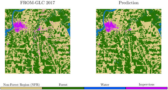
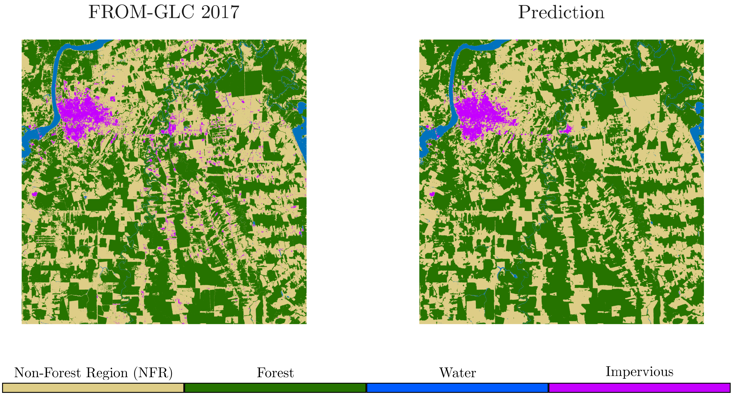
Finally, Figure 10 shows the model’s land cover classification with respect to the FROM-GLC thematic map. It can be seen that the semantic context is well translated into the predictions, although the difference in resolution between the reference and the input features is still visible in smaller details such as roads and narrow river streams. In particular, several smaller clusters from impervious are missed when compared to the ground truth.

Figure 10. Land cover predictions over a zoomed-in Sentinel-1 test scene with respect to the FROM-GLC 2017 reference when considering four classes of interest.

3.2. Systematic Rainforest Monitoring

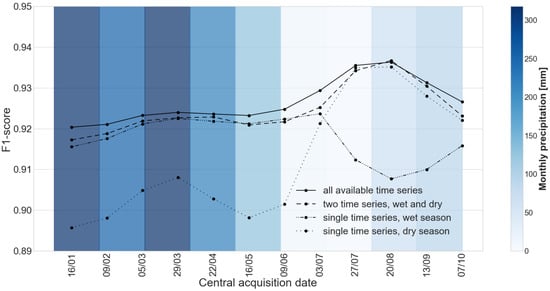
The results are summarized in Figure 11 in terms of overall F₁-Scores. Initial tests show that under the baseline conditions (when a single time series from the wet season is used per footprint for training and validation), the proposed approach still maintains an accuracy above 90% for the external reference throughout the whole observation period.

Figure 11. F₁-Scores for different time series along 2017 based on the number of time series (TS) per footprint available for training and validation. The months highlighted in darker tones of blue are associated with higher monthly rainfall.

However, the seasonal effects on the input data shown in Figure 3 are still reflected in the performance of such year-round forest map generation. For instance, the baseline model trained on the FROM-GLC reference with a time series that comes from the wet season only shows a clear drop in performance starting from July. When the training data come only from the dry season (period typically used to define the optical-based reference maps), the predictions during the wet season are correspondingly affected. Indeed, the SAR backscatter fluctuations observed in Figure 3 suggest that this behavior could be related to the high seasonal variabilities seen over this region, in a way that both SAR and InSAR features might be affected by precipitation and water accumulation on the surface. These intraclass seasonal patterns might lead to confusion if not properly learned by the classification model. In the case of the baseline model, even though the land cover classes are more separable during the dry season, the classifier still fails to generalize due to the lack of appropriate examples during training.

Next, we further evaluate the impact of seasonal sampling on the robustness of the classification model. Figure 11 illustrates the importance of building a dataset which has proper temporal (i.e., seasonal) representativity, as the best performance can be achieved along the year when the complete sequence of time series is used for training. Nevertheless, we show that our deep learning model already reaches a comparable performance by considering only two time series during training, representing the wet season and the dry season, respectively. This indicates that the network can already learn the different seasonal patterns and converge to a better and more stable performance by only seeing each seasonal representation once. Finally, it should be noted that the F₁-Score curves shown in Figure 11 have been estimated as the mean of five runs with pseudorandom seeds. In terms of stability, the worst-case scenario observed in the wet season was a difference on the order of 0.005 in performance, while for the dry season, it was on the order of 0.002 only.

3.3. Post-Classification Analysis and the Role of External References

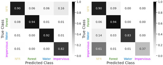
Next, we analyze in greater detail the remaining gaps and potential of this forest monitoring system. Thus, we investigate sources of misclassifications based on the confusion matrices in Figure 12 with respect to the FROM-GLC reference. The confusion matrix on the left-hand side is normalized by column (i.e., predicted class), with the values on the main diagonal expressing the precision metric from Equation (5). It can be seen that, overall, the model achieves a high precision, and most misclassifications involve the so-called negative class, i.e., non-forest regions (NFRs), which is by definition a grouping of several smaller land cover classes. On the other hand, the confusion matrix on the right-hand side is normalized by row (i.e., true class), and represents the recall metric from Equation (6) on its main diagonal. As expected, the classes which are underrepresented during the training phase, i.e., water and impervious, are subsequently underestimated in the test. In particular, the impervious class achieves a recall of only 37%, being classified mostly as NFR otherwise. This could also be explained by the fact that the input feature that contributes the most to discriminate impervious from other classes is the coherence (as in Figure 4), which in turn has the coarser nominal spatial resolution. Finally, the majority of training samples for the impervious class are extracted from larger pixel clusters, and therefore, even though large cities are accurately classified as shown in Figure 10, scattered impervious occurrences can be missed, leading to low recall.

Figure 12. Confusion matrices of FROM-GLC tests, normalized by predicted class (left) and true class (right).

Moreover, some of the confusion between classes might occur due to the simplified definition of the classes of interest. For instance, wetlands typically belong to the NFR, but might be predicted as water depending on flooding conditions. An analogous ambiguity may occur with shrubs, whose lower and sparser vegetation can display physical properties that fluctuate between grasslands and forests. Finally, mines and sparse human settlements share characteristics of impervious for constructed areas, NFR for bare soil and dirt roads, and even forests for highly vegetated villages and ranches.

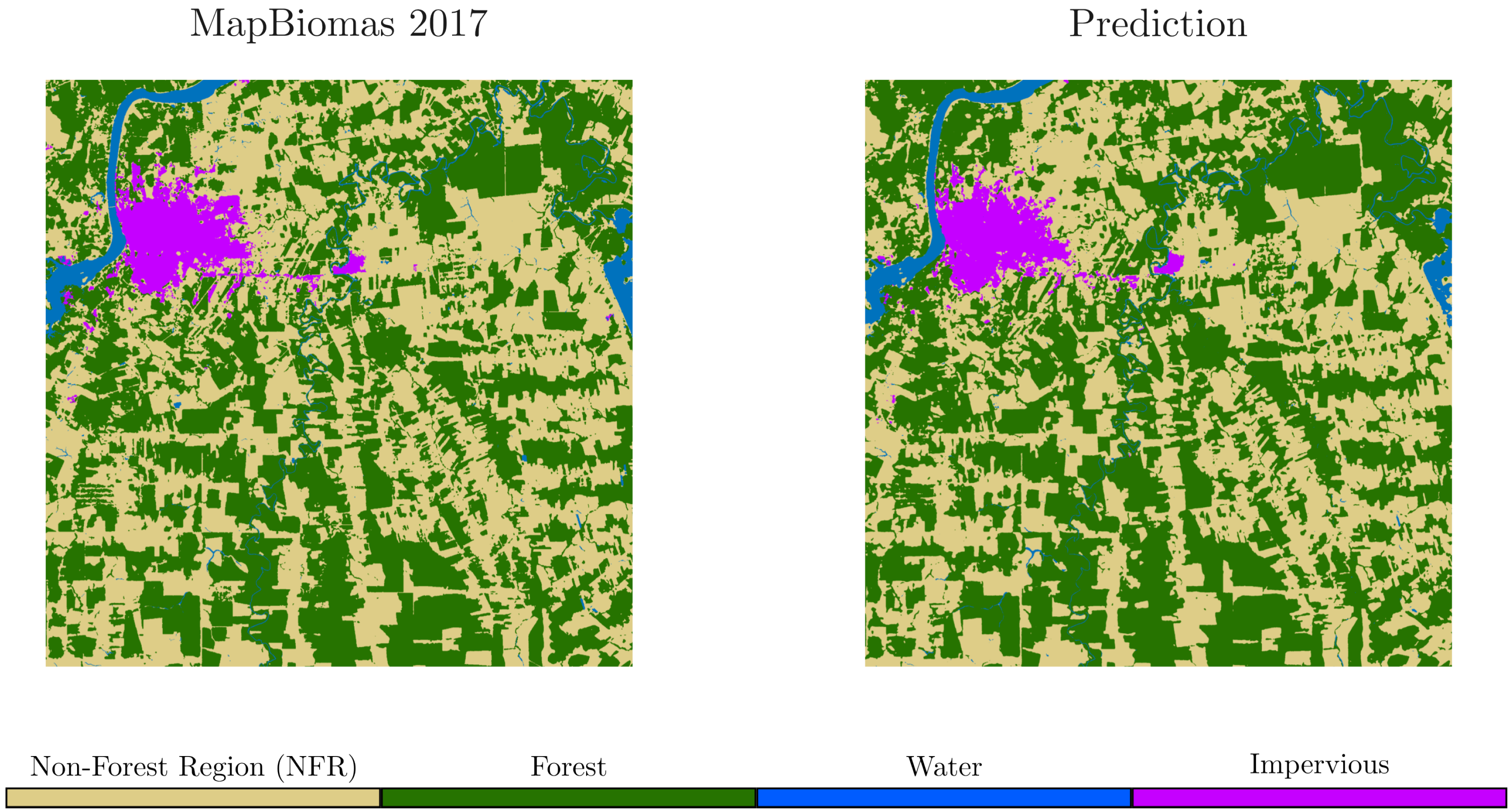
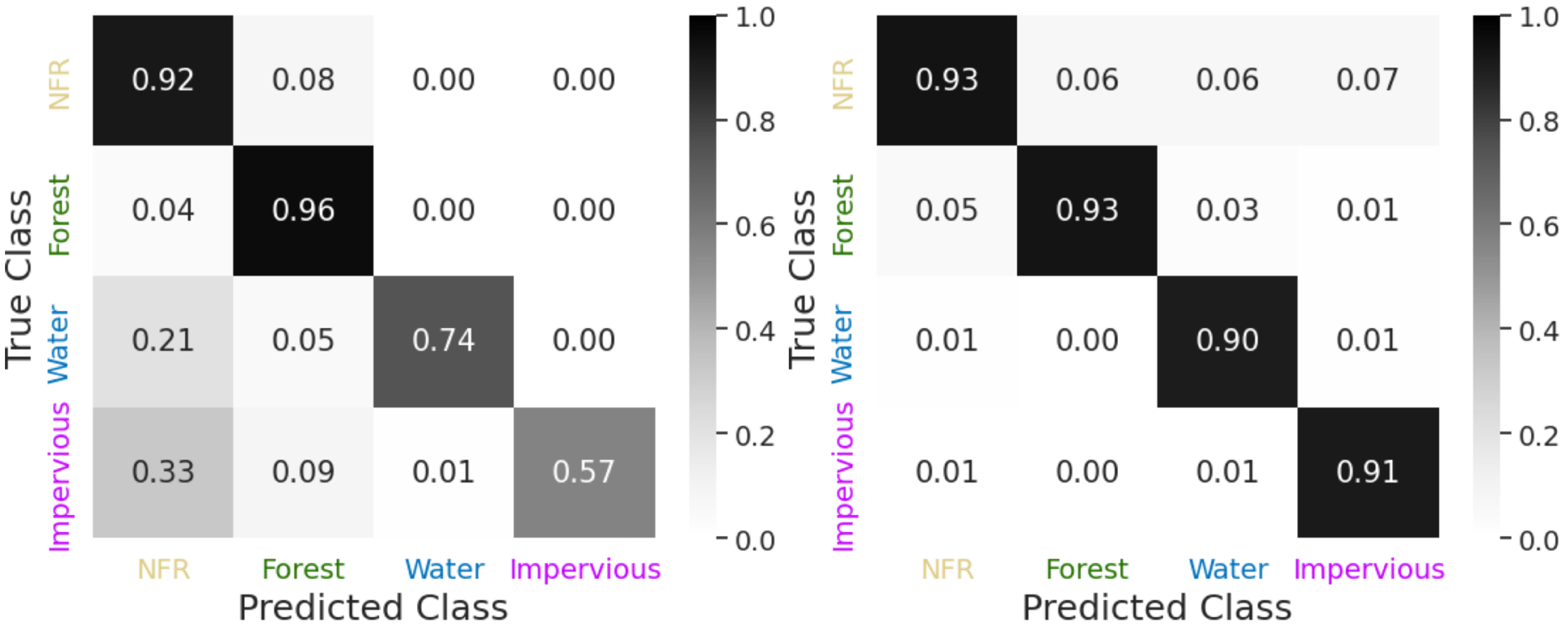
In this context, we perform an intercomparison analysis with a second land cover map, MapBiomas, to investigate the impact of the ground truth on the network’s learning and, therefore, its prediction patterns. Therefore, we train the model from scratch based on this reference and assess its performance following the methodology defined for the FROM-GLC. Figure 13 and Figure 14 show a zoomed-in prediction and the confusion matrix, respectively, when considering the MapBiomas ground truth.

Figure 13. Land cover predictions over a zoomed-in Sentinel-1 test scene with respect to the MapBiomas reference when considering the same class groupings as for the FROM-GLC.

Figure 14. Confusion matrices of MapBiomas tests, normalized by predicted class (left) and true class (right).

It can be observed that by employing MapBiomas as reference data, the overall accuracy performance can be increased by up to three percentage points. This can be explained first by the fact that MapBiomas has been specifically generated for this region, thus being also validated locally and less prone to inconsistencies; and second, MapBiomas has a higher number and more detailed description of the classes, which optimizes the final class grouping into forest, water, impervious, and NFR. Moreover, as can be seen when comparing the FROM-GLC and MapBiomas maps in Figure 13 and Figure 10, respectively, the two references exhibit different ground truths, in particular with respect to impervious areas.

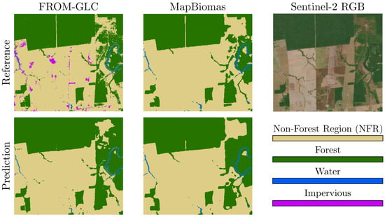
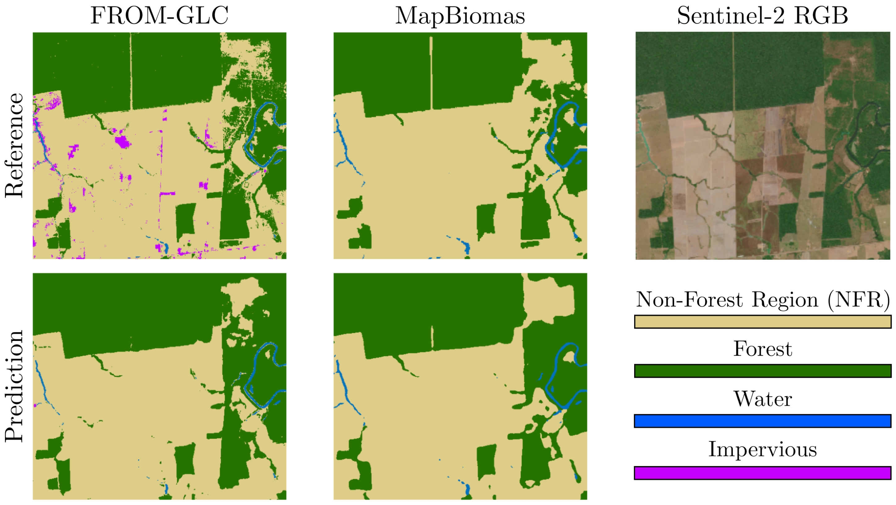
A comparison between both land cover maps and a true color Sentinel-2 image (bands B4, B3 and B2) from July 2017 is shown in Figure 15. Although the FROM-GLC reference has a finer nominal resolution due to the use of Sentinel-2 imagery at 10 m, the MapBiomas map appears to have a more accurate definition of impervious surfaces, as the area of interest mostly contains agropastoral fields in addition to forest. This is reflected in the predictions, where in this case, the classification based on FROM-GLC exhibits a higher level of detail but a lower agreement with its reference compared to the MapBiomas case study.

Figure 15. FROM-GLC and MapBiomas 2017 land cover maps and their respective predictions in comparison to a Sentinel-2 RGB image acquired in July 2017.

4. Discussion

In Section 3.2, we showed that with the proposed deep learning framework and adequate seasonal sampling, we can generate land cover maps over the rainforest on a monthly basis with an overall accuracy around 90% compared to the ground truth. However, there are a series of challenges related to the detection and validation of land cover changes over time. First, the available references are typically generated once per year. For training, this can be partially addressed with the selection of stable areas and the use of deforestation masks to reach ground truths that hold for different time series.

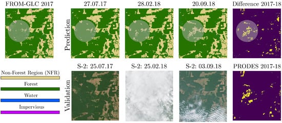
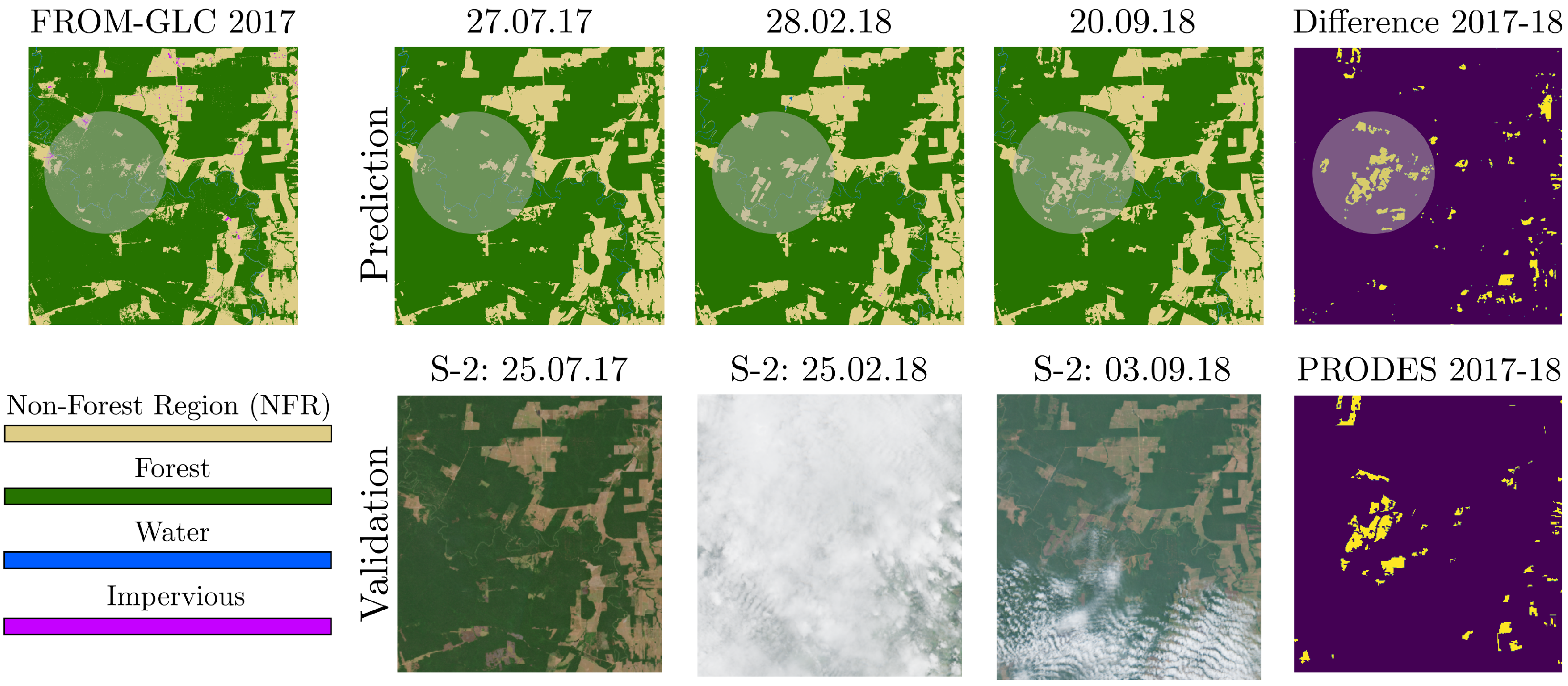
Moreover, there is still a large gap in the validation of the results obtained with SAR during the wet season on a large scale. Given the high classification performance and stability of our model as shown in Figure 11, we can use the proposed method to monitor land cover changes of interest (i.e., deforestation) despite the constraints related to the references. Figure 16 shows the classification of two scenes between July 2017 and September 2018. The dates have been chosen in a manner that ensures cloud-free optical images are available for comparison, while still encompassing the time span in which the PRODES deforestation mask was compiled with data from the dry season. It can be seen through visual inspection that the predictions follow the deforestation trends seen in PRODES, indicating that some of these deforestation focuses could be detected in the early stages with the proposed approach. However, optical satellite imagery, which is still the main data source for monitoring this region, is covered most of the year. This is illustrated in Figure 16, where the deforested area highlighted in the circle can already be identified in February, the peak of the wet season, while it would take months for the verification with cloud-free Sentinel-2 (S-2) images. Moreover, we call attention to the fact that such maps can be generated without overlap on a monthly basis.

Figure 16. Evolution in time of the classified land cover based on the FROM-GLC reference. The predictions suggest that land cover changes observed on the PRODES deforestation mask and Sentinel-2 (S-2) optical images can be detected with the proposed approach.

Finally, it should be noted that the land cover class predictions presented for each Sentinel-1 time series are done independently; i.e., previous results do not affect future decisions. In terms of continuous monitoring, this means that some results might not be consistent in terms of land cover (e.g., a pixel being classified as forest, then NFR, and finally as forest again within a time span of a few months). Thus, for long-term monitoring, spatial–temporal filtering rules could be used to quantify or qualify the changes observed along dense time series with high temporal resolution. Alternatively, a framework with a certain predictive “memory” could help isolate permanent land cover changes from temporary fluctuations affected by noise. In both cases, the availability of timely and accurate validation data during the wet season is still an open problem for effectively monitoring the rainforest.

5. Conclusions

In this paper, we investigated the potential and challenges of monitoring areas of environmental interest such as forests, in particular the Amazon rainforest, with short time series of Sentinel-1 IW data. The proposed approach has demonstrated the potential of SAR in bridging the gap between optical satellite imagery and a consistent monitoring of an area severely affected by cloud cover, although further tests are needed for assessing the model’s robustness to different years and regions. We showed that although extreme seasonal variations can increase ambiguities and uncertainty over land cover classification, a proper dataset generation combined with deep learning tools is capable of addressing these challenges and achieving a robust performance throughout the year when compared to the considered ground truth.

The aforementioned findings, together with the need to undertake deforestation risk assessment and mitigation measures, highlight the potential of the proposed framework as a year-round forest monitoring tool. Nevertheless, there are still a series of challenges to be addressed in future works. First, there is a lack of validation data that meet both spatial and temporal resolution requirements on a large scale. Moreover, external references over the study areas are prone to inaccuracies that affect supervised learning methods and thus classification performance. Finally, although we are able to generate forest maps in near real time, i.e., every 24 days, a sequence of predictions might be needed to increase confidence in potential land cover changes and forest disturbance.

References

- National Institute for Space Research (INPE). Monitoring Program of the Amazon and Other Biomes: Deforestation—Legal Amazon. Available online: https://terrabrasilis.dpi.inpe.br/ (accessed on 11 March 2025).
- Goetz, S.J.; Hansen, M.; Houghton, R.A.; Walker, W.; Laporte, N.; Busch, J. Measurement and monitoring needs, capabilities and potential for addressing reduced emissions from deforestation and forest degradation under REDD+. Environ. Res. Lett. 2015, 10, 123001. [Google Scholar] [CrossRef] [Scilit]
- Shimabukuro, Y.E.; Santos, J.; Formaggio, A.; Duarte, V.; Rudorff, B.; Achard, F.; Hansen, M. The Brazilian Amazon monitoring program: PRODES and DETER projects. In Global Forest Monitoring from Earth Observation; CRC Press: Boca Raton, FL, USA; Taylor & Francis Group: Boca Raton, FL, USA, 2012; Volume 2012, pp. 153–169. [Google Scholar]
- Almeida, C.A.d.; Coutinho, A.C.; Esquerdo, J.C.D.M.; Adami, M.; Venturieri, A.; Diniz, C.G.; Dessay, N.; Durieux, L.; Gomes, A.R. High spatial resolution land use and land cover mapping of the Brazilian Legal Amazon in 2008 using Landsat-5/TM and MODIS data. Acta Amaz. 2016, 46, 291–302. [Google Scholar] [CrossRef] [Scilit]
- Souza, C.M.; Z. Shimbo, J.; Rosa, M.R.; Parente, L.L.; A. Alencar, A.; Rudorff, B.F.T.; Hasenack, H.; Matsumoto, M.; G. Ferreira, L.; Souza-Filho, P.W.M.; et al. Reconstructing Three Decades of Land Use and Land Cover Changes in Brazilian Biomes with Landsat Archive and Earth Engine. Remote Sens. 2020, 12, 2735. [Google Scholar] [CrossRef] [Scilit]
- Pulella, A.; Aragão Santos, R.; Sica, F.; Posovszky, P.; Rizzoli, P. Multi-Temporal Sentinel-1 Backscatter and Coherence for Rainforest Mapping. Remote Sens. 2020, 12, 847. [Google Scholar] [CrossRef] [Scilit]
- Sica, F.; Pulella, A.; Nannini, M.; Pinheiro, M.; Rizzoli, P. Repeat-pass SAR interferometry for land cover classification: A methodology using Sentinel-1 Short-Time-Series. Remote Sens. Environ. 2019, 232, 111277. [Google Scholar] [CrossRef] [Scilit]
- Borlaf-Mena, I.; Badea, O.; Tanase, M.A. Assessing the Utility of Sentinel-1 Coherence Time Series for Temperate and Tropical Forest Mapping. Remote Sens. 2021, 13, 4814. [Google Scholar] [CrossRef] [Scilit]
- Dal Molin, R.; Rizzoli, P. Potential of Convolutional Neural Networks for Forest Mapping Using Sentinel-1 Interferometric Short Time Series. Remote Sens. 2022, 14, 1381. [Google Scholar] [CrossRef] [Scilit]
- Doblas, J.; Shimabukuro, Y.; Sant’Anna, S.; Carneiro, A.; Aragão, L.; Almeida, C. Optimizing Near Real-Time Detection of Deforestation on Tropical Rainforests Using Sentinel-1 Data. Remote Sens. 2020, 12, 3922. [Google Scholar] [CrossRef] [Scilit]
- Hansen, J.N.; Mitchard, E.T.A.; King, S. Assessing Forest/Non-Forest Separability Using Sentinel-1 C-Band Synthetic Aperture Radar. Remote Sens. 2020, 12, 1899. [Google Scholar] [CrossRef] [Scilit]
- Voormansik, K.; Zalite, K.; Sünter, I.; Tamm, T.; Koppel, K.; Verro, T.; Brauns, A.; Jakovels, D.; Praks, J. Separability of Mowing and Ploughing Events on Short Temporal Baseline Sentinel-1 Coherence Time Series. Remote Sens. 2020, 12, 3784. [Google Scholar] [CrossRef] [Scilit]
- Ronneberger, O.; Fischer, P.; Brox, T. U-Net: Convolutional Networks for Biomedical Image Segmentation. In Proceedings of the Medical Image Computing and Computer-Assisted Intervention—MICCAI 2015, Munich, Germany, 5–9 October 2015; Navab, N., Hornegger, J., Wells, W.M., Frangi, A.F., Eds.; Springer: Cham, Switzerland, 2015; pp. 234–241. [Google Scholar]
- Batistella, M.; Robeson, S.; Moran, E. Settlement Design, Forest Fragmentation, and Landscape Change in Rondonia, Amazonia. Photogramm. Eng. Remote Sens. 2003, 69, 805–812. [Google Scholar] [CrossRef] [Scilit]
- Guild, L.S.; Cohen, W.B.; Kauffman, J.B. Detection of deforestation and land conversion in Rondônia, Brazil using change detection techniques. Int. J. Remote Sens. 2004, 25, 731–750. [Google Scholar] [CrossRef] [Scilit]
- Pedlowski, M.A.; Dale, V.H.; Matricardi, E.A.; da Silva Filho, E.P. Patterns and impacts of deforestation in Rondônia, Brazil. Landsc. Urban Plan. 1997, 38, 149–157. [Google Scholar] [CrossRef] [Scilit]
- de Barros Ferraz, S.F.; Vettorazzi, C.A.; Theobald, D.M.; Ballester, M.V.R. Landscape dynamics of Amazonian deforestation between 1984 and 2002 in central Rondônia, Brazil: Assessment and future scenarios. For. Ecol. Manag. 2005, 204, 69–85. [Google Scholar] [CrossRef] [Scilit]
- Gong, P.; Wang, J.; Yu, L.; Zhao, Y.; Zhao, Y.; Liang, L.; Niu, Z.; Huang, X.; Fu, H.; Liu, S.; et al. Finer resolution observation and monitoring of global land cover: First mapping results with Landsat TM and ETM+ data. Int. J. Remote Sens. 2013, 34, 48. [Google Scholar] [CrossRef] [Scilit]
- Gong, P.; Liu, H.; Zhang, M.; Li, C.; Wang, J.; Huang, H.; Clinton, N.; Ji, L.; Li, W.; Bai, Y.; et al. Stable classification with limited sample: Transferring a 30-m resolution sample set collected in 2015 to mapping 10-m resolution global land cover in 2017. Sci. Bull. 2019, 64, 370–373. [Google Scholar] [CrossRef] [Scilit]
- de Almeida, C.A.; Maurano, L.E.P.; de Morisson Valeriano, D.; Camara, G.; Vinhas, L.; Gomes, A.R.; Monteiro, A.M.V.; de Almeida Souza, A.A.; Rennó, C.D.; Silva, D.E.; et al. Methodology for Forest Monitoring used in PRODES and DETER Projects. CEP 2021, 12, 010. [Google Scholar]
- Krieger, G.; Moreira, A.; Fiedler, H.; Hajnsek, I.; Werner, M.; Younis, M.; Zink, M. TanDEM-X: A satellite formation for high-resolution SAR interferometry. IEEE Trans. Geosci. Remote Sens. 2007, 45, 3317–3341. [Google Scholar] [CrossRef] [Scilit]
- Prats, P.; Rodriguez-Cassola, M.; Marotti, L.; Nannini, M.; Wollstadt, S.; Schulze, D.; Tous-Ramon, N.; Younis, M.; Krieger, G.; Reigber, A. TAXI: A Versatile Processing Chain for Experimental TanDEM-X Product Evaluation. In Proceedings of the IEEE Geoscience and Remote Sensing Symposium, Honolulu, HI, USA, 25–30 July 2010; pp. 1–4. [Google Scholar]
- Yague-Martinez, N.; Prats-Iraola, P.; Gonzalez, F.R.; Brcic, R.; Shau, R.; Geudtner, D.; Eineder, M.; Bamler, R. Interferometric processing of Sentinel-1 TOPS data. IEEE Trans. Geosci. Remote Sens. 2016, 54, 2220–2234. [Google Scholar] [CrossRef] [Scilit]
- Touzi, R.; Lopes, A.; Bruniquel, J.; Vachon, P.W. Coherence estimation for SAR imagery. IEEE Trans. Geosci. Remote Sens. 1999, 37, 135–149. [Google Scholar] [CrossRef] [Scilit]
- Funk, C.; Peterson, P.; Landsfeld, M.; Pedreros, D.H.; Verdin, J.P.; Shukla, S.; Husak, G.; Rowland, J.; Harrison, L.; Hoell, A.; et al. The climate hazards infrared precipitation with stations—A new environmental record for monitoring extremes. Sci. Data 2015, 2, 150066. [Google Scholar] [CrossRef] [Scilit] [PubMed]
- Goddard Earth Sciences (GES) Data and Information Services Center (DISC). FLDAS Noah Land Surface Model L4 Global Monthly 0.1 × 0.1 Degree (MERRA-2 and CHIRPS); Goddard Earth Sciences (GES) Data and Information Services Center (DISC): Greenbelt, MD, USA, 2018. [CrossRef]
- Kingma, D.; Ba, J. Adam: A Method for Stochastic Optimization. In Proceedings of the International Conference on Learning Representations, San Diego, CA, USA, 7–9 May 2014. [Google Scholar]
Disclaimer/Publisher’s Note: The statements, opinions and data contained in all publications are solely those of the individual author(s) and contributor(s) and not of MDPI and/or the editor(s). MDPI and/or the editor(s) disclaim responsibility for any injury to people or property resulting from any ideas, methods, instructions or products referred to in the content. |
© 2026 by the authors. Licensee MDPI, Basel, Switzerland. This article is an open access article distributed under the terms and conditions of the Creative Commons Attribution (CC BY) license.