


Highlights
What are the main findings?
- Peatland-wide phenology trends broke in 2020–2021, with lengthening seasons and higher greenness until 2020, shorter seasons in 2021, and partial recovery after.
- Vegetation patches show differences in their responses and dependence: (i) Sphagnum-Carex mats had the longest seasons but the weakest hydroclimatic links; (ii) Phragmites mats showed the shortest and most variable seasons; (iii) willow forests were the most stable; (iv) transitional zones were the most hydrology-sensitive.
What are the implications of the main findings?
- Temperature dominates EVI across patches. Meanwhile, phase-aligned water-table depth and precipitation windows better predict phenology than annual means, requiring site-specific phenophase averages.
- High-resolution satellite monitoring is essential for detecting nonlinear vegetation reorganisation in drying peatlands and informing targeted conservation of functional regions.
Abstract
Current climatic conditions are drying peatland ecosystems, compromising carbon storage through increased decomposition and vegetation shifts. Large-scale monitoring is essential to quantify climate change impacts on vegetation and hydrology. PlanetScope high-resolution imagery (3 m pixel) over seven years (2017–2023) served as proof-of-concept for a central European peatland (Rzecin, Poland). The enhanced vegetation index (EVI) was selected based on ground validation (R = 0.9 vs. 0.8 for NDVI-normalised vegetation index). Phenological metrics (SOS—start of the season; EOS—end of the season; LOS—length of the season; POS—peak of the season; EVImax; amplitude; area) were derived via DATimeS from snow-free EVI time series. Trends were analysed using pixel-wise slopes, change-point detection (break ~2020–2021), paired correlations, subarea (P1–P4) behaviour, and PCA, alongside air temperature (Tair), precipitation, and water table depth (WTD). Results revealed LOS and peak EVI increased until 2020, a 2021 break, and a 2022–2023 recovery, signalling nonlinear vegetation reorganisation. Transitional mire floating mats (Sphagnum spp.–Carex spp.–Vaccinium oxycoccus) showed the longest seasons/highest greenness but weakest hydrometeorological links, implying rising internal dynamics. Phragmites mats, fern–sedge edges, and riparian willow differed in tolerance or sensitivity to WTD and precipitation oscillations. Tair dominated EVI seasonality across types, while WTD and precipitation controlled phenology and greenness in edges, showing better results with phase-aligned means. Vascular plants outpaced mosses in peak EVI and persistence, with patch-specific shifts.
1. Introduction
Peatlands sustain the global carbon cycle, acting as reservoirs for around 40% of the terrestrial carbon stored in soils [1]. The vegetation is one of the main drivers of this cycle, determining the amount of atmospheric CO2 sequestered into plant biomass [2]. Over the past few decades, the water table depth (WTD) oscillations have become more extreme due to climate change, leading to an anticipated drying of the peatland’s ecosystem that could result in shifts in vegetation composition [3,4]. The new climatic conditions destabilised these ecosystems, potentially transforming them from carbon sinks to carbon sources [5]. Furthermore, their drying makes them more susceptible to fires, which would release more carbon into the atmosphere. Their importance in the global carbon cycle and the need for their conservation and restoration make improving our understanding of peatland adaptation to climatic conditions crucial [6]. Beyond its impact on the carbon cycle, vegetation phenology changes also serve as climate change indicators [3]. For these reasons, monitoring changes in vegetation phenology and cover is important for estimating the consequences of climate change.
Peatlands are considered ecosystems with high heterogeneity of vegetation, particularly in the case of poor fens [7]. Satellites usually provide ≥10 m spatial resolution, which may be insufficient to detect the heterogeneity of peatlands’ vegetation. The challenge of analysing vegetation phenology in peatlands stems not only from their heterogeneous vegetation but also from their high water content and periodic waterlogging, which, among other factors, contribute to more haze episodes than typically observed in different areas. However, high-resolution satellites, such as the PlanetScope ensemble with 3 m/pixel resolution, allow more accurate identification of vegetation patches and their growing seasons. The use of PlanetScope across multiple growing seasons, ecosystem types, and climate domains has proven effective in capturing fine-scale spatial variation in vegetation phenology that is not resolved at moderate spatial resolutions, making it a recommended tool for studying canopy-scale phenology [8]. Moreover, PlanetScope’s revisit time is less than 2 days, with multiple images available daily, allowing the user to obtain at least two images per month despite haze. This approach, using new high-resolution imagery, can improve estimations of vegetation phenology and vegetation index oscillations, thereby increasing our understanding of their dynamics and responses to climate change.
Studying the dynamics of different vegetation classes and their coupling with air temperature and WTD measurements enhances our understanding of seasonal patterns and the long-term impacts of climate change, providing valuable insights into peatland hydrological and phenological dynamics. Therefore, in this study, we examined the impact of ongoing climate change on vegetation phenology and their different responses in the Central European Rzecin peatland using a time series of high-resolution satellite imagery and on-site WTD and meteorological measurements. The novelty of this work lies in combining PlanetScope imagery with in situ data to study long-term phenological changes in vegetation, a topic that has not been addressed in this area. This integrated analysis provides new insights into the hydrometeorological influences on vegetation phenology across the entire Rzecin peatland and its different vegetation subareas based on vegetation types. The expected results considering the continuous drop in WTD observed in the area are (i) a general enlargement of the length of the growing season and increased greenness with the proliferation of vascular plants; (ii) a higher dependence on WTD’s changes in the transitional areas of the peatland with mixed vegetation including mosses; (iii) a more direct link with meteorology in the areas with a more stable dominance of shrubs and vascular plants, with the vegetation shift not masking the link with vegetation indexes.
2. Materials and Methods
2.1. Study Area
The Rzecin area is crucial for regional nature conservation, supporting diverse vegetation, including brown mosses, Sphagnum, and various species of vascular plants. In the area, 26 rare and endangered species and 20 locally threatened species can be found [9].
The peatland provides varied ecological conditions with differences in fertility and water availability, fostering a rich biodiversity of 127 vascular plant species from 84 genera and 43 families, 17 of which are on the Regional Red List. Additionally, 34 moss taxa from 10 families, including endangered species like Sphagnum fuscum and Paludella squarrosa, contribute to the site’s ecological significance [9,10]. Human activity has significantly altered the development of the Rzecin peatland over the past two centuries. Between 1880 and 1890, deforestation and the construction of the Rzecin drainage canal initiated major alterations in the wetland ecosystem, leading to habitat acidification and changes in hydrology [9,10].
The Rzecin peatland is a large (87 ha) mesotrophic, geogenous wetland, a poor-rich fen (area code Natura 2000: PLH300019) located in Western Poland (52°45′N latitude, 16°18′E longitude, 54 m a.s.l.) [7,11]. In the centre of the peatland, an approximately 70 cm thick floating mat of peat substrate is present. In contrast, the peat surface is more anchored to the bedrock through the periphery, producing differences in vegetation and deeper WTD [11]. Due to the presence of a floating mat, the WTD seasonal dynamics are much less in the middle of the peatland with a higher WTD position than at its edge, determining the dominance of Sphagnum spp., Carex rostrata, Carex limosa, Eriophorum angustifolium and Oxycoccus pallustris in the middle of the peatland. At its edge, the dominant plant communities are composed of taller vascular plants such as Phragmites australis, Typha latifolia, Carex elata and Salix spp. [11].
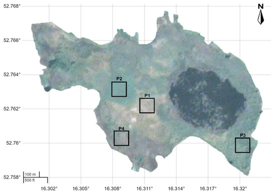
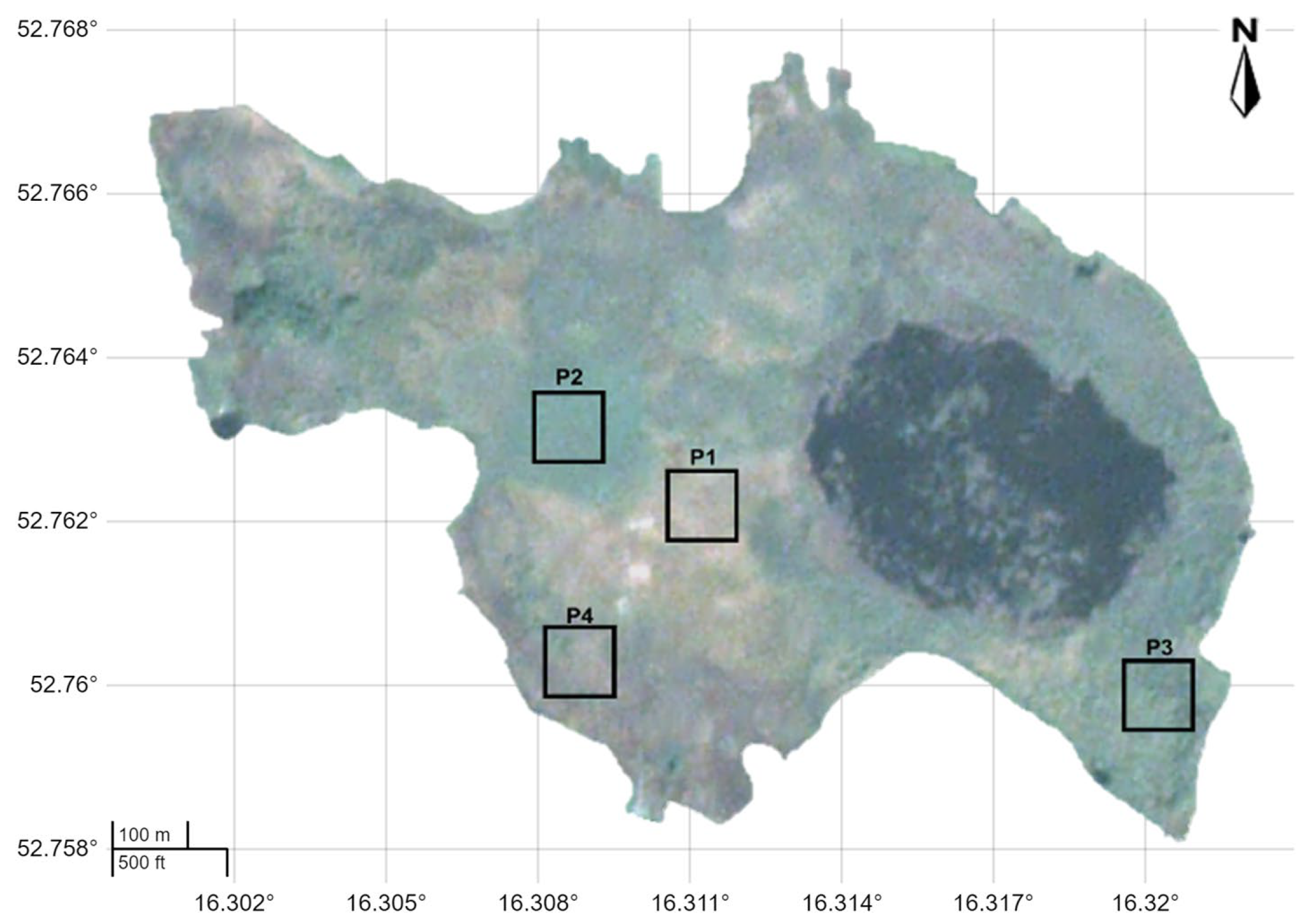
The vegetation distribution used in this article is based on the vegetation classifications done in the area [12] and represented in Figures S1–S3. Due to differences in area among classes, this study selects four subareas within the classification with equal dimensions to represent the different vegetation communities and their locations (Figure 1, Table 1). In each subarea, specifications describe the vegetation groups, generic types and plant communities based on the area/polygon groups from Figures S1–S3, while the detailed plant community information is based on the specific vegetation found in the subarea. The patch dimensions are 93 m × 93 m, corresponding to 31 × 31 pixels in PlanetScope images, and would be ~3 × 3 pixels if using Landsat 8 (30 m/pixel), significantly reducing the detection of spatial variation in the canopy.
Figure 1.
Rzecin peatland RGB scene generated from PlanetScope 07/2023 image. Black rectangles locate vegetation patches (P1–P4).
Table 1.
Specifications of each subarea selected. Note that all classifications come from the vegetation surveys made in the peatland area during 2019 [12].
2.2. Satellite Imagery
The satellite dataset used in this study was the PlanetScope high-resolution (3 m/pixel) satellite ensemble, comprising 144 images across four reflectance bands from 2017 to 2023. The product used was the PlanetScope Ortho Scene, an analytic surface reflectance. The OrthoScenes are radiometrically and geometrically corrected products projected to a WGS84 Web Mercator cartographic map projection with a positional accuracy of less than 10 m Root Mean Square Error (RMSE) at the 90th percentile. The four bands (B1—Blue, B2—Green, B3—Red, B4—NIR) were harmonised with Sentinel 2 using the PlanetScope Application Programming Interface (API) Orders and Tools (Planet Labs PBC). Only the images with the highest publishing stage (finalised) and quality category (standard) were included, ensuring optimal radiometric consistency and minimal processing artefacts. Furthermore, the images were anchored to the same scene using the API’s correction tools to ensure geometric consistency. From the available ~3200 images of the Dove Classic (PS2) and Dove R (PS2.SD) instruments, the used imagery was selected based on cloud cover below 10%; haze was also a criterion for exclusion. The images that had more than 5% snow-flagged PlanetScope pixels, identified by the UDM2 mask as regions covered with snow/ice, were also discarded. Further technical details, including radiometric calibration methods and spectral band specifications, are available in the PlanetScope Product (Specification Planet Labs PBC 2023 Combined Imagery Product Spec FINAL | December 2023 (https://assets.planet.com/docs/Planet_Combined_Imagery_Product_Specs_letter_screen.pdf - accessed 3 February 2024)).
2.3. In Situ Data
In situ data measured in the study area included WTD measurements obtained using TD-divers (Eijkelkamp Soil & Water, Giesbeek, GL, The Netherlands) installed in polyvinyl chloride (PVC) tubes permanently mounted to wooden platforms stabilised on piles above the peatland surface. The WTD position was calculated as the difference between the distance from the top edge of the piezometer to the TD-Diver installation depth and the distance from the top edge of the piezometer to the peatland surface [7]. Due to seasonal fluctuations in the peatland surface, its position was determined from manual measurements of the distance between a fixed point on the platform and the peatland surface, taken every 2–3 weeks. Changes in the peatland surface were then linearly interpolated between measurements and incorporated into WTD calculations.
The air temperature (Tair) was measured with radiation-sheltered HygroVue5 thermohygrometers (Campbell Scientific, Logan, UT, USA). The measurements provide a continuous dataset with half-hourly timesteps throughout the study period [7]. In situ measurements of precipitation and WTD began at the end of 2017; therefore, the time series will not include these two parameters’ data before 2018.
2.4. Vegetation Indices Calculation and Selection
The satellite data was used to generate the enhanced vegetation index (EVI) [13] and the Normalised Difference Vegetation Index (NDVI) [14]. These indices include the near-infrared (NIR) and red (RED) reflectance channels to capture the vegetation red edge peak, enabling differentiation of vegetation types and phenological status through contrast between chlorophyll absorption in red and high NIR scattering by healthy leaf mesophyll [14]. Additionally, EVI incorporates a blue channel correction factor and additional ratio terms to minimise soil background, atmospheric, and aerosol influences, providing more robust sensitivity in complex environments like wetlands, where water saturation and litter affect the spectral signals [13].
The selection of vegetation indices (VIs) for phenological calculations was based on agreement between ground VIs calculated from periodic top-of-canopy reflectance measurements (FieldSpec HandHeld 2, ASD Inc., Boulder, CO, USA) and satellite-derived VIs at each ground point location. The 18 ground points used were located in the Rzecin experimental station described in Juszczak et al. [15] during 42 field campaigns in 2018–2021.
2.5. Vegetation Phenological Parameters
The identification of vegetation phenological variables (SOS—start of the season; EOS—end of the season; LOS—length of the season; peak of the season—POS; maximum value of EVI—EVImax; amplitude—Amp; and area) was generated with Decomposition and Analysis of Time Series (DATimeS) software 1.13 [16] using the VI selected. SOS, POS, EOS and LOS parameters describe the seasonal distribution and duration within the year, the EVImax identifies the maximum value of the index, the amplitude represents the distance between the bottom and the peak of the seasonal curve, and the area represents the area behind the seasonal curve. Whittaker interpolation was applied to the EVI snowless images time series to obtain the index’s daily values. The interpolated time series was then used to retrieve phenological parameters for each year and analyse changes and trends in the overall area. DATimeS identifies the growing seasons from the time series, detecting three consecutive local minimum, maximum and minimum points with specified constraints to avoid noise interferences [16]. The constraints used were the growing season prominence (set to 20%) and the minimum separation between seasons (set to 100). Once the growing season is identified, DATimeS estimates the phenological parameters based on the seasonal, relative or absolute amplitude [16]. In this case, the seasonal amplitude was used and set to 25%. The EOS and SOS were selected “where the left/right part of the curve reaches a fraction of the seasonal amplitude along the rising/decaying part of the curve.” The overall calculations produced images of each year’s phenological parameters, along with average area values. Parallelly, phenological variables were generated for the selected vegetation patches (P1–P4; Figure 1).
2.6. Statistical Analyses of Time-Series Relationship (Vegetation Phenological Parameters, WTD, Precipitation and Tair)
All statistical analyses were performed in MATLAB (The MathWorks, Inc., Natick, MA, USA) and RStudio (Posit team, Boston, MA, USA). For each patch and vegetation class, phenological parameters were also extracted. To observe differences in the patches’ phenology beyond visually analysing time-series trends and linking the results to vegetation-class trends, a PCA was performed in RStudio, with the results displayed as a biplot.
The analysis of phenological trends and changes within the time series was first performed by calculating the slope for each parameter and dividing the study period into two. To identify the temporal shifts, a change-point analysis was applied separately to each pixel and each phenological parameter. Only series with at least five non-missing years were analysed. The change point was estimated using the “findchangepts” function in MATLAB (MathWorks, Natick, MA, USA) with MaxNumChanges = 1, returning at most one break year per pixel and variable. To obtain a single, robust break-year surface, the seven parameter-specific break maps were combined by computing the mean break year per pixel across all phenological variables, ignoring missing values, and rounding to the nearest integer year. The result is a composite break-year map representing the average timing of structural change across the phenological cycle. Once the break year was calculated, the differences between the distinct peatland areas classified by vegetation type and between patches were analysed by calculating, pixel-wise, the slope before and after the break year for the entire peatland area using a first-degree polynomial fit. Additionally, the slope for the whole period was also calculated. The behaviour of the phenological parameters in pairs was also analysed using pixel-wise correlations over the entire period.
From the correlations and slope maps, averages and standard deviations per class and area were calculated and exported as tables. Moreover, the results were evaluated for normality with the Lilliefors test, and, if normal, a combination of ANOVA and Tukey tests was applied to identify differences; otherwise, a combination of Kruskal–Wallis and Dunn tests was used for the same purpose. The groups were labelled with letters, and their distributions were shown in boxplots per class and area.
The partial least squares regression (PLSR) method was used to analyse the relationships of WTD, Tair, and precipitation with the EVI and vegetation phenological parameters. The significance of the PLSR results was estimated from the linear regression between modelled and measured values. PLSR was applied with the “plsregress” MATLAB function. The PLSR models relationships between predictor variables (X—hydrometeorology) and response variables (Y—EVI) while handling multicollinearity and high-dimensional data [17]. Firstly, it extracts latent components (PLS components) that maximise the covariance between X (predictors) and Y (response). The extracted components are used to build a predictive model for Y, and by analysing the Variable Importance in Projection (VIP) scores, PLSR determines the contribution of each predictor to the response variable [17]. PLSR (adjusted for three PLS components) was applied to each vegetation patch and the general area, using all hydrometeorological variables to obtain VIP scores and the total percentage of EVI variance explained. Moreover, to obtain the individual percentages explained by each hydrometeorological variable, PLSR was applied separately to WTD, Tair, and precipitation, adjusted to one PLS component.
The analysis of the effect on phenology included the estimation of the average and total values of meteorological variables for the entire year and for phenological periods. The phenological-period averages/sums were from the 30 days prior to the EOS, SOS, and POS, plus the averages/sums during the season. In a first step, the two best averages/sums for each hydrometeorological parameter type (Tair, WTD, and precipitation) were selected based on the VIP scores in the PLSR using all values. The PLSR for each phenological variable was then calculated for individual pairings (air temperatures, precipitation, WTDs vs. phenology) and for the overall model (hydrometeorology vs. phenology). The results were illustrated using heatmaps of the phenology variance explained by hydrometeorology, obtained from PLSR.
For the area-averaged EVI–hydrometeorology relationship, the analysis was performed at daily, weekly, and monthly timesteps. To further study the effect, a cross-correlation analysis was performed, pairing EVI with WTD, Tair, and precipitation at daily, weekly, and monthly timesteps (averaged except for precipitation, which was summed). Once cross-correlation was performed and the lag between time series was obtained, the time series were displaced, and PLSR was performed in the same way for phenology, both pairwise and overall.
3. Results
3.1. General Trends of the Vegetation Season Parameters in the Peatland Area
The robustness of satellite EVI values was higher than that of satellite NDVI values in the 18 ground points. EVI showed higher similarity with in situ data than NDVI (NDVI—R = 0.8, p-value = 4.1 × 10⁻⁶, RMSE = 0.09; EVI—R = 0.9, p-value = 1.5 × 10⁻⁷, RMSE = 0.08, Figure S4). Based on these results, EVI was used to analyse vegetation phenological parameters.
The peatland showed a general increase in the length of the vegetation season from 2018 to 2020. The LOS changes were caused by the delay of the end of the season from late October to early November, while the SOS remained stable around the end of April (±5 days) until 2021, when it was delayed to 12 May (Table 2). The prolongation of the vegetation season during these years was accompanied by the delay of the POS from the 1st week of July 2018 to the 1st week of August 2020, with a stable peak value of EVI (0.4663 ± 0.0167). Starting from 2021, the POS remained stable around the 3rd week of July, while the EVI value rose by around 0.1. In 2021, the LOS dropped drastically from 192 to 157 days (Table 2) due to a cold spring and dry spells during July–August and October. The pattern of prolonging the season length, broken in 2021, was recovered in 2022–2023. There was an increase in the LOS, with the SOS returning to late April and the EOS progressively returning to early November (Table 2). Moreover, the maximum value of EVI (EVImax) started to decrease in 2021, and the peak date remained around 25 July ± 5 days (Table 2).
Table 2.
The peatland area’s average length of the season (LOS) expressed in days, the start and end of the season (SOS, EOS), and the maximum value of the enhanced vegetation index (EVImax) with the peak of the season (POS) date.
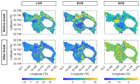
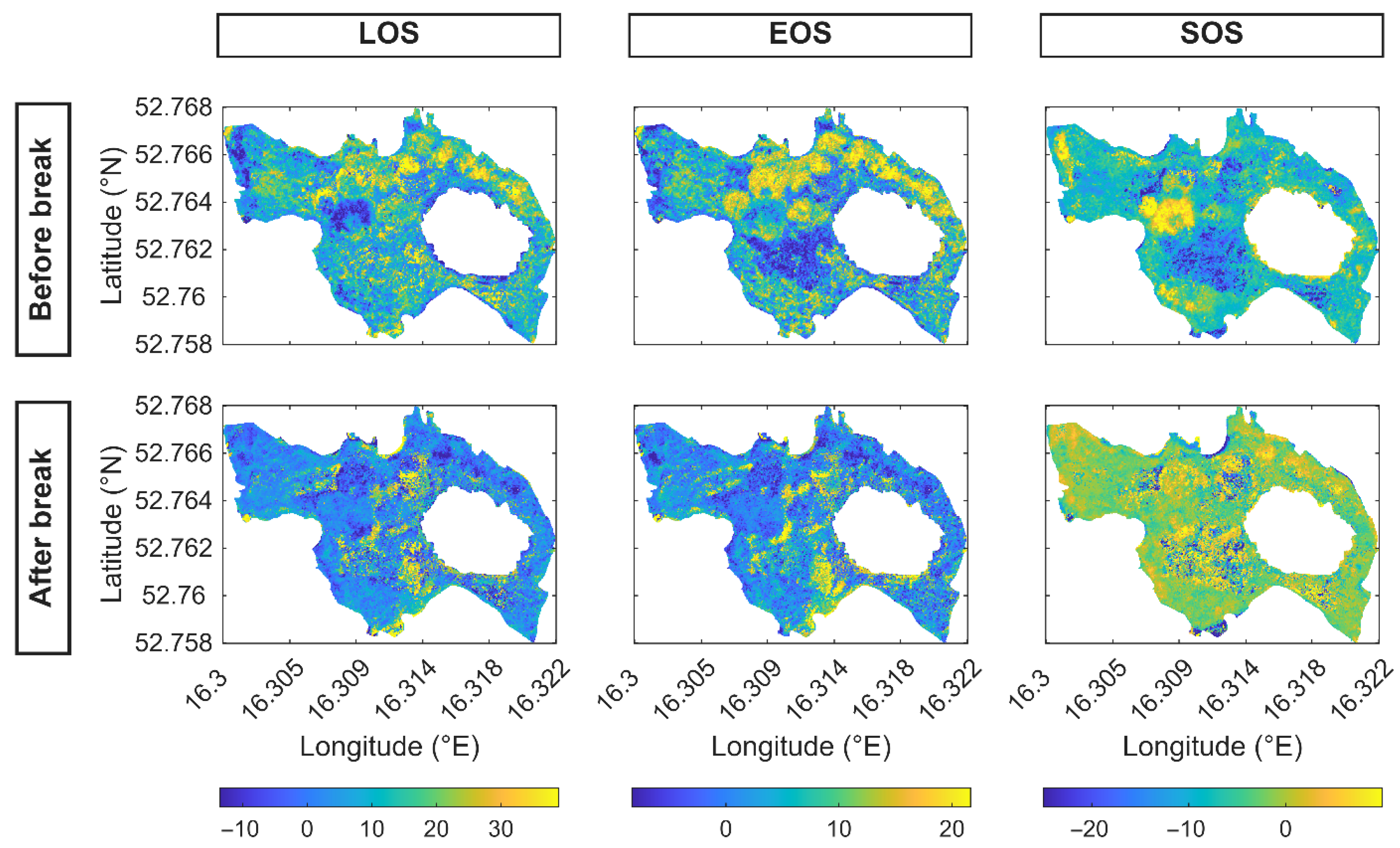
Despite hints from the average phenological parameter indicating a phenological trend break in 2021, pixel-wise, the change began mainly in 2020. Most of the peatland underwent a rapid change in phenological variables starting in 2020, with only isolated patches of vegetation showing the largest changes in 2019 or 2021 (Figure S5). During the first period studied, LOS, EOS, and POS increased. Hence, inducing larger seasons and delayed EOS and POS, while SOS tended to be earlier (Figure 2 and Figure S6). The second period shifted the dynamics, and most of the peatland area showed patterns of minor changes at the start and end of the season, and consequently in LOS with mainly earlier POS (Figure 2 and Figure S6). Some spatial patterns were visible, e.g., some of the transitional mire regions showed the most advanced EOS and SOS only before the break year (Figure 2, Figures S3 and S7), the areas with the presence of Typha spp. and Phragmites spp. had the highest positive slopes in EOS and SOS before the break year, while it was the areas with the presence of Sphagnum spp. after the break year in this case, in EOS and LOS (Figures S8 and S9).
Figure 2.
Start of the season (SOS), length of the season (LOS) and end of the season (EOS) slopes from the years 2017–2023, divided into 2 periods by the identified break year (Figure S5). The slopes are expressed as the original data magnitude, days of the year (DOY).
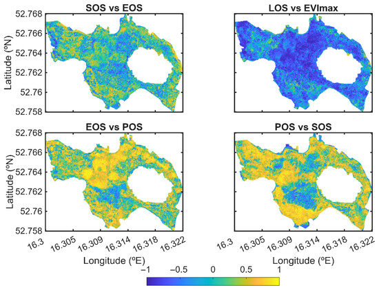
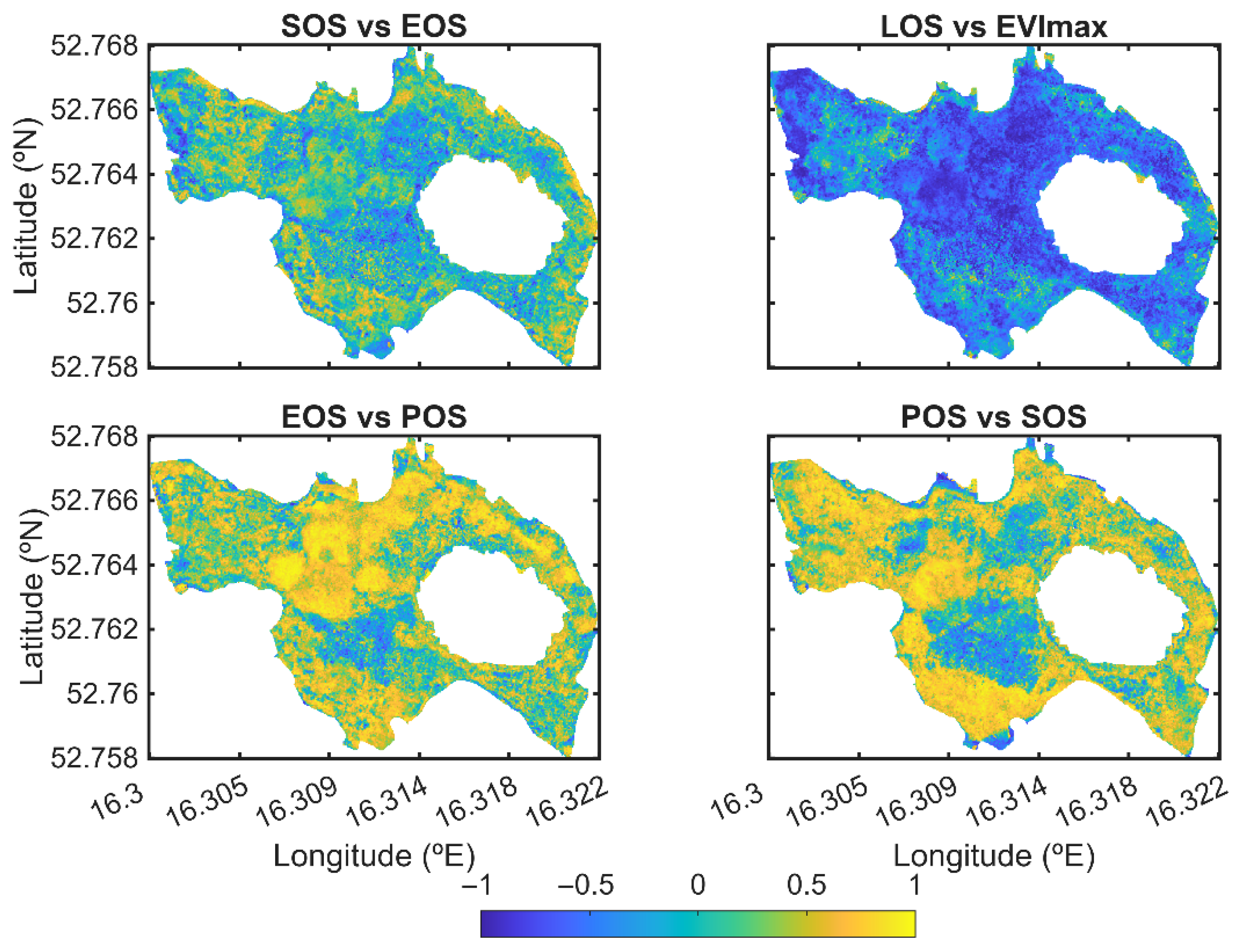
The correlation between phenological parameters indicated that, in general, most of the area showed a positive relationship between the end and start of the season, with both advancing or delaying together (Figure 3). The correlations between EOS, SOS and the seasonal peak were similar, with overall positive links. However, the analysis also showed that peak EVI values were negatively associated with LOS, indicating that, as with EVImax vs. amplitude, areas with higher seasonal greenup variability (amplitude) and longer growing seasons tend to have lower EVI peaks (Figure 3 and Figure S10). Spatially, the main “big” areas highlighted were seen in the EOS vs. POS and the POS vs. SOS correlation results (Figure 3 and Figure S11). These areas were broadly classified as transitional mire regions of the Rzecin peatland with mixed vegetation species (Figure S1), visible as the greener “triangular” area observed around 52.762–52.76°N 16.309–16.314°E in the bottom subplots of Figure 3.
Figure 3.
Pixel-wise correlation of the phenological parameters estimated from the enhanced vegetation index (EVI) pairwise from the years 2017–2023. Parameters paired: start of the season (SOS), length of the season (LOS), end of the season (EOS), peak of the season (POS) and the EVI value during POS (EVImax).
3.2. Phenology of Vegetation Patches and Its Link with Vegetation Classes
The changes in vegetation phenology did not follow the same trend in all the peatland areas, as shown in Figure 1 and generally explained in the previous section. These differences were further analysed using the selected vegetation patches (Figure 1). Over the seven-year period, the peatland subsites exhibited apparent differences in both the timing and magnitude of phenological parameters (Figure 2).
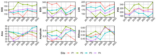
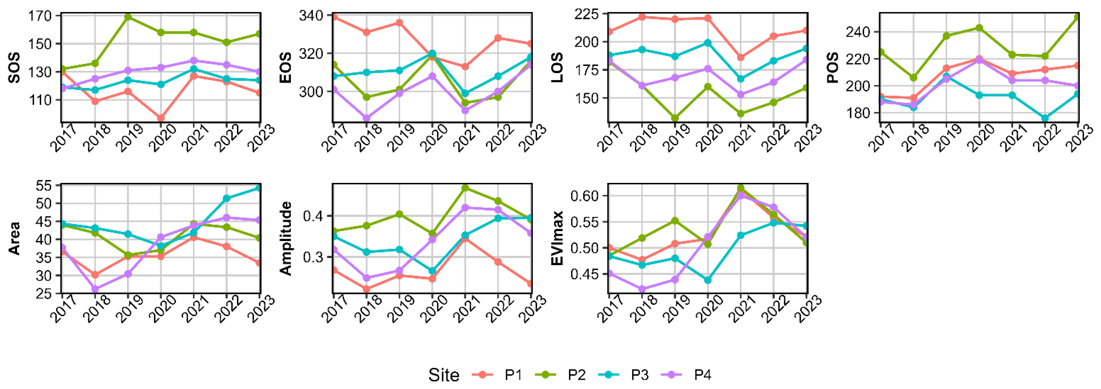
In P1, the growing season typically began earlier and ended later than for other subsites, resulting in a consistently long season length (LOS; Figure 4). The area under the EVI curve, as well as the seasonal maximum (EVImax), remained high throughout, suggesting persistent and strong canopy growth; amplitude varied more modestly (Figure 4). SOS and EOS generally advanced during 2017–2020, while LOS remained largely stable. After 2021, LOS increased, driven by later EOS and earlier SOS, recovering from the 2021 drop. The area and amplitude peaked in 2021 and right after decreased toward previous values (Figure 4).
Figure 4.
Phenological parameters per site during the study period (2017–2023) based on the enhanced vegetation index (EVI). The start, end and peak of the season SOS, EOS, and POS are expressed as day of the year (DOY). The length of the season (LOS) is expressed in days, and EVImax (maximum EVI) is unitless.
P2, the Phragmites-dominated subsite, was characterised by the latest SOS, the highest POS values, and overall, the shortest seasons (Figure 4). LOS and productivity, as measured by area and amplitude, decreased from 2019 to 2021, with some improvement afterwards (Figure 4). SOS in P2 shifted to later dates up to 2019, then began to occur earlier (Figure 4). These patterns suggest sensitivity to local water regime changes or annual climate variation.
P3, dominated by tall shrubs, had SOS values often close to those of P1 but did not reach such long seasons (Figure 4). POS advanced steadily from 2019 onwards, while amplitude and area generally increased across the study period (Figure 4). EOS behaved similarly to P2 and P4 in some years (Figure 4). P4’s season also started early but ended earlier than P3, resulting in a shorter LOS (Figure 4). For P4, amplitude and area rose towards the end of the period, and SOS remained consistently stable between years (Figure 4).
Compared to the general peatland mean, P3 and P4 most closely matched the composite behaviour in both timing (SOS, EOS, LOS) and productivity (area, EVImax, amplitude). In contrast, P1 exhibited the longest and earliest seasons, whereas P2’s season was typically later and more variable, making these subsites less representative of the general pattern (Figure 4).
The behaviour of regions with mosses showed a general drop of LOS with later SOS and mixed EOS oscillations depending on the area (though the average slope was negative—earlier EOS), while POS advanced (Figures S8 and S9). Mosses also showed one of the lowest correlations between SOS/EOS and POS, and, together with perennial grasses and pine forest areas, the strongest relationship between seasonal length and the maximum EVI (Figures S12 and S13). P1, a subarea with moss presence, showed similar trends, a detachment of EOS and SOS with POS trend (due to POS stability) and the reverse link between EVImax and LOS with shorter seasons and higher EVI (Figure 4).
Similarly, the regions of perennial grasses, also found in P2, showed mainly a drop in LOS, with lower variability than mosses and higher average values (closer to 0 days slope), which was still non-significantly different in trend from mosses (Figure S8). In this case, the shortening of LOS was mainly due to a slightly bigger displacement of SOS than EOS, though both were generally delayed. Despite inter-annual oscillations, P2 showed this same trend with SOS changing more than EOS (slope-wise) and, as mentioned, previously the negative relationship between LOS and EVImax showed by perennial grasses was also visible in P2 trends (Figure 4).
The willow regions showed the highest agreement within the pixel-wise changes, with the lowest area variability in LOS, EOS, SOS, and POS changes (together with the pine forest). There were also delays in EOS and SOS, with seasonal lengths showing low variations. This was the same as for P3, the most stable site analysed, with the POS being more linked to SOS than EOS (Figure 4 and Figure S8).
The ferns, an area in which P4 was partially located, together with mosses, showed the highest pixel-wise variation in the EOS and LOS slope over the studied period, indicating that the changes were not uniform across the areas. Ferns showed LOS changes similar to those of mosses, with slopes that did not differ significantly within these groups. However, in this case, both EOS and SOS were more delayed than in the moss regions, and POS followed similar trends, producing higher correlations of POS, EOS, and SOS (Figure S8). P4 was located in a transitional zone with sedge, which is why it did not clearly follow the fern patterns as in the previous cases. These two vegetation groups differ significantly in all paired correlations analysed and in LOS, EOS, SOS, and POS, with the only similarity being the SOS changes after the break year (Figures S8 and S12).
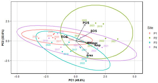
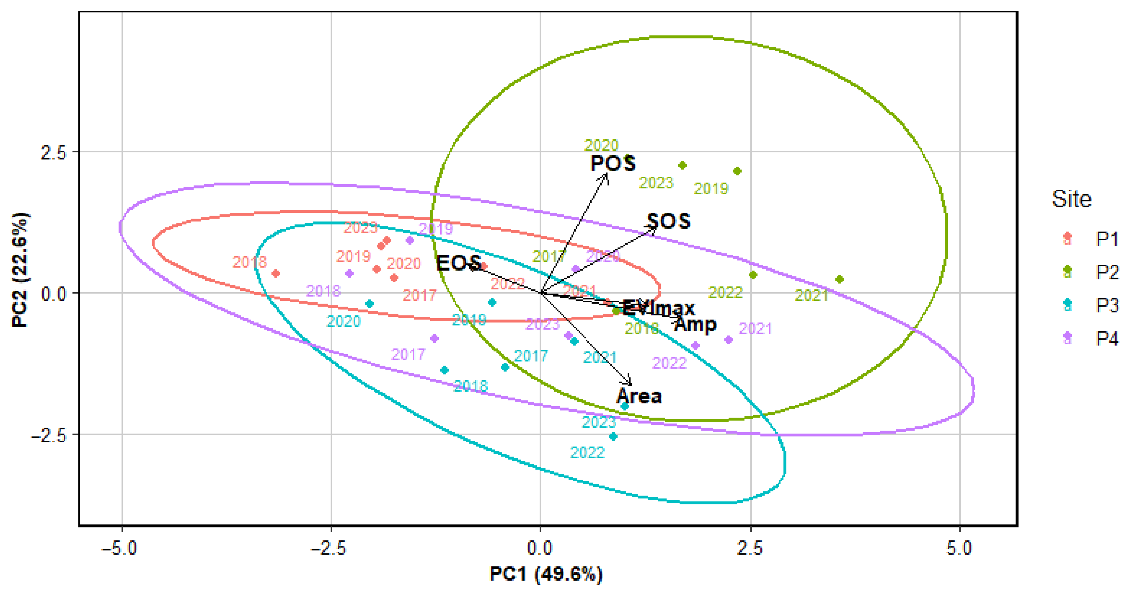
The analysis of the phenological parameters with PCA (Figure 5) revealed that most of the variance among patches was explained by a combination of season length (LOS), total seasonal productivity (area), and amplitude. P1 and P2 were clearly separated along the first principal component, indicating their different strategies: longer, more productive seasons with higher amplitude in P1 versus shorter, less productive seasons in P2. P3 and P4 occupied intermediate positions but demonstrated increasing productivity (area and EVImax) and phenological flexibility over time (SOS, POS, and EOS changes). The second principal component further highlighted differences in the timing of key season events, particularly the relative lateness of P2’s SOS and POS compared to earlier and more stable timing in P3 and P4. The annual dispersion of points within each patch reflected the degree of phenological plasticity or environmental sensitivity, with sites like P2 showing broader interannual spread.
Figure 5.
Biplot of the principal components analysis per subsite (P1–P4) of the phenological parameters estimated for the study period (2017–2023) based on the enhanced vegetation index (EVI), where the start, peak, and end of the season (SOS, EOS, POS) unit is day of the year (DOY). LOS or the length of the season is expressed in days, EVImax or the maximum EVI and the amplitude (Amp) and area parameters are unitless.
Altogether, these results demonstrate that the peatland subsites differ in how their vegetation responds, both in the timing and strength of seasonal activity, highlighting spatial variation in ecological function and potential responses to hydrological and climatic variability. However, when the phenological parameters of all years were analysed together to group the patches studied, due to the variability of their values, they always shared at least a part of their distributions and hence characteristics, without a significant difference based on the statistical results (Figure S14). P2 showed differences from the other areas in SOS and POS values, and significant differences in LOS across all subareas except P4. P1 showed significant differences in EOS and LOS values (Figure S14). Meanwhile, P3 and P4, in all cases, shared some portion of their distribution, with no significant differences, as well as sometimes with P1 and P2.
3.3. The Role of Hydrometeorological Variables
3.3.1. EVI Changes
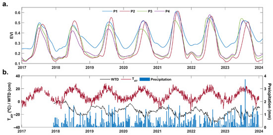
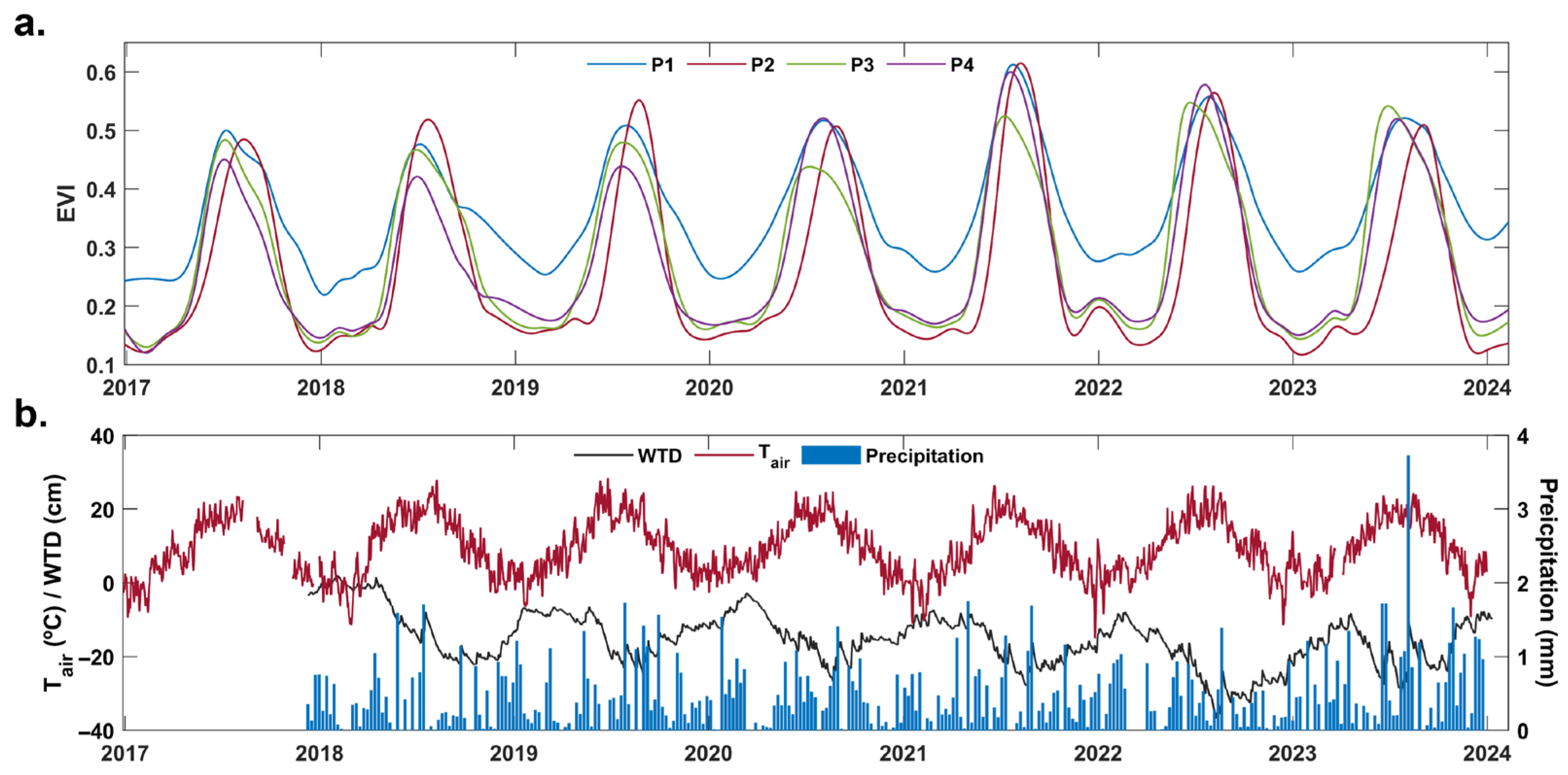
The shared trends in hydrometeorological variables and the EVI, averaged per patch or across the total study area, are visible in Figure 6, along with the time series of EVI values (Figure 6a) and their linkage with air temperature and WTD (Figure 6b). EVI trends and air temperature show a Gaussian shape peaking during the summer (Figure 6). At the same time, for the WTD interannual trend, the link with EVI is observed in the opposite direction (the lowest WTD is associated with Tair and EVI peaks) and with a time lag (Figure 6).
Figure 6.
Time series of daily enhanced vegetation index (EVI) for patches of different vegetation P1–P4 (a), and time series of daily air temperature (Tair, dark red), daily average water table depth (WTD, black), and weekly cumulative precipitation (blue columns) (b). Note that (a) presents only a primary y-axis and the right ticks represent the same EVI values.
Further analysis of the role of each variable in EVI trends revealed lagged responses of EVI to changes in hydrometeorological variables across the different areas. The cross-correlation analysis in weekly and monthly timesteps revealed a delay in the reaction of EVI to WTD changes but not to air temperature and precipitation oscillations (Tables S5 and S6). The delay or lag varied across vegetation patches. The maximum lag in the EVI response was detected in P2, followed by P1, the general area, P4, and P3 (Table 3). The lag in the EVI response decreased as the data timestep increased, smoothing the distinction between vegetation areas. Weekly WTD averages showed the same lag in P1 and the general peatland area, and monthly averages showed the same lag across all areas (Table 3).
Table 3.
EVI delay in response to changes in water table depth (WTD) based on the maximum cross-correlation. The delay is expressed in days for daily data, weeks for weekly data and months for monthly data. Note that 2017 was excluded from analyses due to missing reliable WTD data. Full cross-correlation results are available in Table S4.
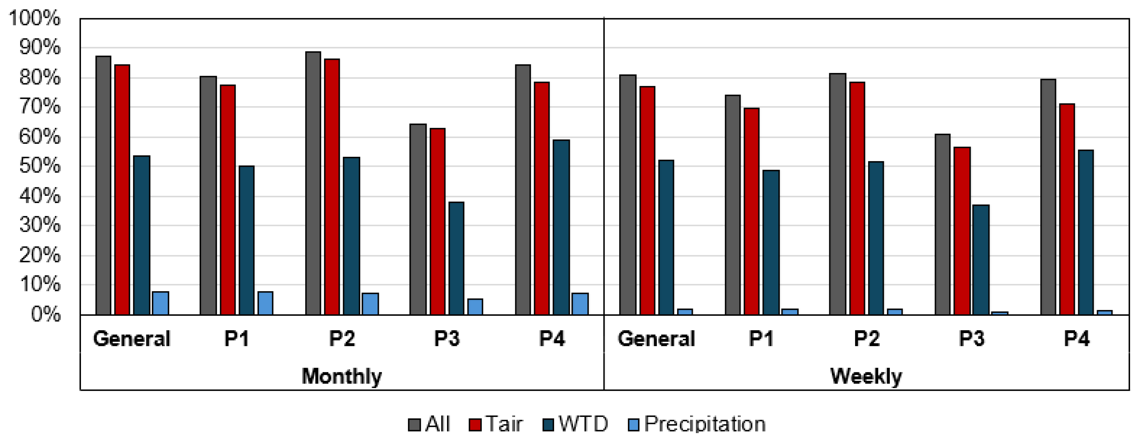
Lags were applied to displace the WTD time series to better analyse the role of each hydrometeorological variable in the PLSR. The results indicated that air temperature governs EVI oscillations, followed by WTD, with precipitation exerting a minimal effect on both the weekly and monthly time series (Figure 7). The role of precipitation increased from weekly to monthly values. However, it was still not significant, explaining less than 10% of the EVI changes and with a VIP score below 0.15 (Figure 7, Table S7). The area where the air temperature was the least important, for a percentage of the variance of EVI explained, and the VIP score was P4 (Figure 7, Table S7). At the same time, P4 was also the area with the highest WTD importance (Figure 7, Table S7).
Figure 7.
Percentage of the enhanced vegetation index (EVI) explained by air temperature (Tair), water-table depth (WTD), and precipitation from the partial least squares regression of these variables individually and together (All), from monthly and weekly values.
The similarity between P1 and the general area lag was again observed in the monthly and weekly VIP scores for Tair and WTD (Table S7). However, precipitation played a greater role in P1. Moreover, the percentage of EVI oscillations explained by individual variables or their combination was lower in P1 than in the general area (Figure 7). In the case of P3, this was true in both timesteps: the area with the least EVI oscillations could be explained by hydrometeorology (Figure 7). P2 was the area where the EVI changes could be explained the most by hydrometeorology (Figure 7).
3.3.2. Changes in Vegetation Phenology
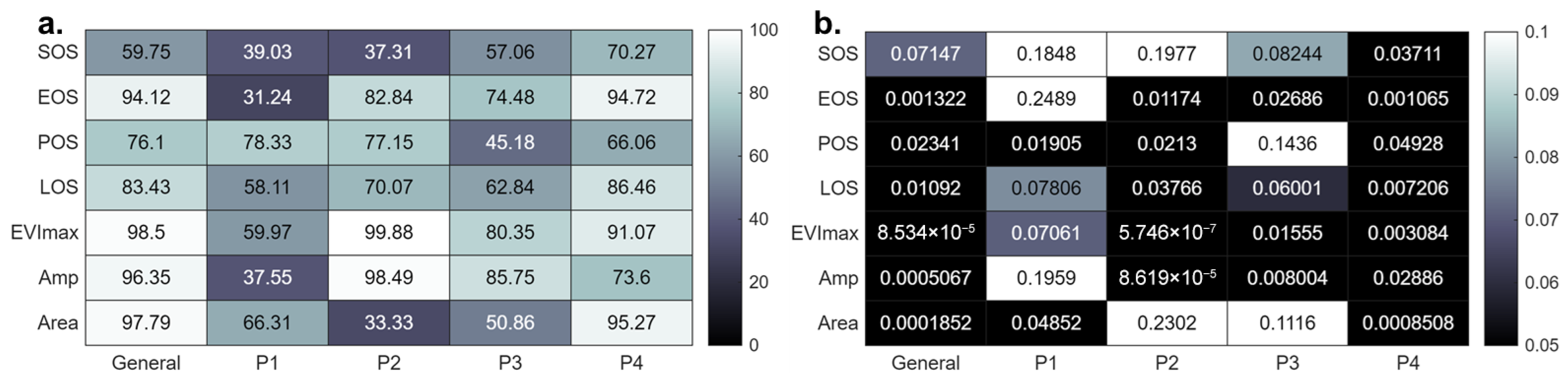
In the general peatland area, phenological parameters were explained by air temperature, WTD, and precipitation in most cases, with at least 50% of their variance accounted for and a significant relationship (Figure 8). However, PLSR also revealed that SOS and area parameters were the most difficult to explain using the chosen hydrometeorological variables, both in annual averages and as a function of the phenological phase. Overall, the best predictors were only significantly related in the case of P4, with SOS variance explained below 60% in the other cases, including the general peatland area (Figure 8). On the patches scale, P1 was the subarea most difficult to predict with SOS, EOS, and amplitude explained variance below 40%, and p-values > 0.05 for all phenological parameters except POS and area (LOS and EVImax could be considered significant with p-values < 0.1). P3 also showed some difficulties with SOS, POS, and area prediction, whereas in P2, the non-significant predictions occurred only in SOS and area values. In contrast, P4 had the highest variance explained and significant links to all phenological variables (Figure 8).
Figure 8.
Results of the partial least squares regression (PLSR) between the enhanced vegetation index (EVI) and air temperature, water-table depth, and precipitation. On the left (a), the percentage of EVI variance explained, and on the right (b), the significance, p-value, from the regression of modelled (PLSR) and measured values.
The changes in phenology trends, as described by the break in 2020–2021, were also observed in air temperature. While the air temperature at the beginning of 2019 and 2020 was generally above 0 °C, it was below 0 °C in 2021, with freezing temperatures occurring more frequently (Figure 6b). In addition, the oscillation of WTD also showed a similar pattern to the changes in vegetation season. While WTD in 2019–2020 remained at a similar yearly average (−13.1 cm, −13.9 cm), it increased during 2021 by ~3 cm (annual average), showing levels that did not reach the surface as in the previous years (Figure 6b, Table S3). From 2021, WTD showed a stronger increasing trend, reaching its lowest point during summer-autumn 2022 and recovering to 2021 levels in 2023 due to increased precipitation (Figure 6b, Table S3). The higher air temperatures and lower WTD were aligned with the increase in the greenness of the patches during 2021 and the general peatland area (Figure 6a,b), while the length of the season was drastically reduced, affected mainly by the changes at the start of the season due to colder conditions (Table S3, Figure 6b).
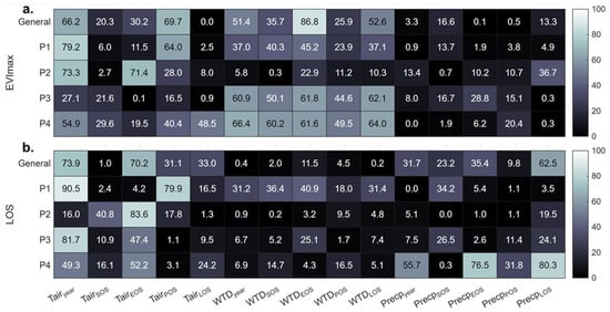
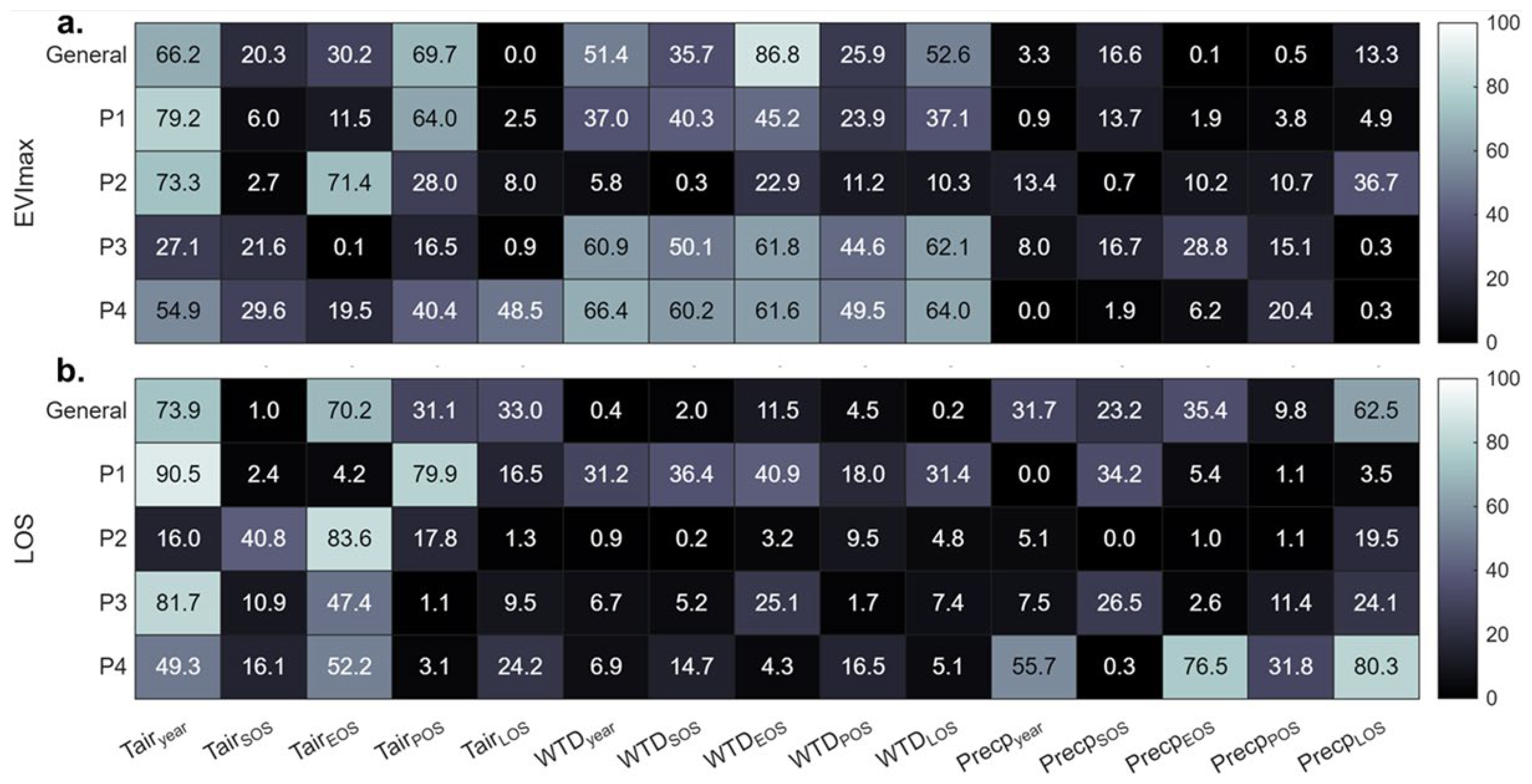
Focusing on the individual role of each meteorological parameter, each patch responded differently, not only in the importance of each variable type but also in the type of average or sum performed (dependent on the phenological phase or the year). Among the floating mat patches (P1 and P2), EVImax was most strongly driven by temperature, with P1 showing the highest explanatory power for both annual and growing-season temperature windows (Figure 9). P2 showed a similar reliance on temperature conditions, but with the strongest response centred on the period around peak season (Figure 9). In both cases, hydrological and precipitation variables generally exhibited much lower explanatory power for EVImax, reinforcing a temperature-driven productivity regime.
Figure 9.
Variance explained (%) of the maximum enhanced vegetation index (EVImax) (a) and length of the season (LOS) (b) by air temperature (Tair), water-table depth (WTD), and precipitation (Precp) values per phenological phase and year. Subscripts of the start, peak, end, and length of the season (SOS, POS, EOS, and LOS) indicate the summaries of variables based on the phenological phases.
In contrast, the non-floating riparian forest patch (P3) displayed a distinct ecophysiological response, with EVImax primarily influenced by water-table depth during the growing season (WTD_LOS, 61.8%) and at the end of the season (WTD_EOS, 60.1%, Figure 9). Here, temperature metrics accounted for much less variance, emphasising the importance of hydrological controls in this patch. Transitional vegetation in P4 exhibited an intermediate pattern, with both temperature (Tair_year, 54.9%) and water-table depth at the end of the season (WTD_EOS, 61.6%) contributing meaningfully to EVImax, but without a single dominant driver (Figure 9).
At the scale of the whole peatland, the patterns largely mirrored the floating mat patches, with temperature and late-season water-table metrics (particularly WTD_EOS, 86.8%) emerging as the strongest controls on EVImax (Figure 9). This likely reflects the broader productivity dominance of these habitats within the peatland complex, while still integrating signals from the hydrologically constrained forest and fern patches.
Considering the length of the growing season (LOS), a similar patch-dependent pattern can be observed. For the general area, LOS was jointly shaped by annual temperature (Tair_year, 73.9%) and end-of-season warmth (Tair_EOS, 70.2%), with a noticeable influence of total season precipitation (Prec_LOS, 62.5%, Figure 9). In P1, LOS was most tightly linked to annual and the average temperature during the season (Tair_year, up to 90.5%), while in P2, the season length was almost exclusively controlled by temperature at the end of the growing season (Tair_EOS, 83.6%, Figure 9). The riparian forest (P3) and transitional patch (P4) exhibited broader climatic sensitivities, with water-table depth (WTD_year and WTD_EOS) and precipitation (Prec_LOS) playing more substantial roles (Figure 9). In P4, the cumulative precipitation during the season was especially influential, explaining up to 80.3% of LOS variance.
Taken together, these results highlight both the spatial heterogeneity and the strong climatic phase specificity in peatland phenology controls. Floating mat patches and the overall peatland area were most responsive to temperature conditions—particularly during the primary and late growing season—while forested and transitional areas show a shift towards WTD and precipitation dependence. The different roles of each variable, depending on the window used to summarise meteorological conditions (e.g., annual, LOS, EOS), emphasise that the timing of climatic effects is as relevant as the driver type. The high complexity of peatland phenology requires site- and phase-specific modelling to accurately capture ecosystem responses to meteorological variability.
4. Discussion
4.1. Peatland-Wide Phenological Trends in the Context of Hydrometeorology, and Vegetation Change
The peatland analysis showed consistent changes in vegetation phenology over the study period, with a progressive increase in LOS and EVImax up to 2020, followed by a marked disruption in 2021 and partial recovery in 2022–2023. The composite break-year analysis located the main shift in phenological trends around 2020–2021 across most of the peatland, indicating a coherent change in season timing at the ecosystem scale rather than isolated local anomalies. Meteorological and hydrological conditions could explain this pattern. According to the IMGW “Climate of Poland” classification, the years 2018–2020 were classified as extremely or anomalously warm, with relatively shallow WTD measured in the study area, whereas 2021 was close to normal (or cooler in spring), characterised by deeper average WTD measurements [18,19]. The continued WTD drawdown in the area has already been reported in other studies [20], while the partial recovery could be associated with increased precipitation.
The LOS increase until 2020 was mainly driven by later EOS, while the break in 2021 resulted from a delayed SOS and earlier EOS, shortening the season despite higher EVImax. This combination of deeper WTD, higher EVImax, and generally longer LOS in most years was consistent with a gradual shift in the balance between moss-rich communities and vascular plants reported in long-term peatland records under drying and warming [21,22]. The following recovery of LOS in 2022–2023, with SOS returning towards late April and EOS extending again into autumn, occurred under conditions of deeper WTD but higher annual precipitation. This suggests that once vascular plants become more dominant, increased precipitation can buffer the negative effects of warm years on LOS, in line with studies showing that higher rainfall can partly offset water-table drawdown effects on peatland vegetation [23]. Overall, the phenology break and subsequent trajectories indicate an interaction between climate anomalies and a gradual reorganisation of plant communities rather than a purely climatic signal [3].
4.2. Patch-Scale Phenological Differences Shaped by Vegetation Composition
Patch-scale analysis revealed that phenological responses differed systematically among vegetation types defined by independent field classification [12]. P1, a floating transitional mire dominated by Sphagnum spp., Carex spp., and Vaccinium oxycoccos, consistently had the earliest SOS and latest EOS, resulting in the longest seasons and high seasonal area and EVImax. P2, a Phragmites-dominated floating mat, showed the latest SOS, highest POS and the shortest LOS, while P3 (riparian willow forest) and P4 (fern–sedge transitional zone) occupied intermediate positions, with P3 being the most phenologically stable across years, as similarly observed in other peatlands [24].
The slope maps and per-patch time series showed that the 2020–2021 break altered the direction or strength of trends in most phenological parameters. Before the break, LOS and EOS generally increased while SOS tended to advance, particularly in floating-mat and transitional areas; after the break, changes in LOS, SOS and EOS were smaller, indicating a partial stabilisation of the system under the new vegetation and hydrological configuration consistent with the literature [3]. Areas mapped as moss-rich or fern-dominated showed the largest spatial variability in LOS and EOS slopes, whereas willow and pine stands had more homogeneous and smaller slope magnitudes, consistent with the greater phenological stability of woody canopies [24,25].
Integrating patch phenology and vegetation classes highlights two important points. First, P3 and P4 most closely tracked the behaviour of the peatland mean, both in timing (SOS, EOS, LOS) and in changes in area, EVImax, and amplitude, whereas P1 and, especially, P2 deviated from the composite pattern. Second, mixed or transitional vegetation (P1, P4) combined long seasons with strong interannual variability in amplitude and area, whereas willow forest (P3) maintained relatively stable EVImax and timing despite shifts in WTD and temperature, as stated by other studies [25]. This supports the idea that vegetation composition, as documented in the field map, underlies the observed phenological heterogeneity rather than purely microclimatic differences [26,27].
4.3. Hydrometeorological Controls on EVI
The EVI time series and cross-correlation analysis showed that air temperature and WTD co-vary with EVI at the seasonal scale, with EVI peaking in summer when Tair is highest and WTD deepest, while EVI responds to WTD with a lag that depends on vegetation type and position within the peatland. Edge patches (P3, P4) had the shortest lags, consistent with their deeper, more variable WTD and transitional character, whereas floating-mat areas (P1, P2) showed longer lags, indicating buffered responses mediated by soil moisture and rooting depth [26,27].
PLSR confirmed that temperature was the primary driver of EVI in the floating-mat patches and for the whole peatland, with WTD and precipitation playing secondary roles that increased towards the margins and in specific phases of the season, as also observed in other studies [2]. In P1 and P2, EVImax was best explained by annual or growing-season temperature windows, with limited additional variance explained by hydrology or rainfall, indicating, as in other studies, a predominantly temperature-driven productivity regime in these mats [3]. In contrast, in P3 (riparian forest), EVImax was more strongly linked to WTD during LOS and EOS than to temperature, reflecting tighter hydrological control in the non-floating forest zone, whereas P4 showed an intermediate pattern with comparable contributions from temperature and WTD at the end of the season [26].
At the peatland scale, the strongest controls on EVImax combined annual temperature and late-season WTD, suggesting that late-season water conditions modulate how much of the temperature signal translates into maintained greenness. These findings are in line with studies reporting strong temperature sensitivity of canopy greenness in boreal and temperate peatlands, modulated by water availability and vegetation type [2,3]. The patch-dependent lags and control strengths demonstrate that even within a small peatland complex, EVI responses to meteorology and hydrology are not uniform and cannot be captured by a single aggregated relationship [28].
4.4. Hydrometeorological Controls on Phenology
When focusing on phenological metrics, the PLSR analyses revealed a more complex, patch-specific pattern than simple annual regressions. For the peatland mean, LOS was jointly shaped by annual and growing-season temperature, end-of-season warmth and, to a lesser extent, cumulative precipitation during the season, while SOS and area were more difficult to predict. Our results show that predictor windows aligned with phenophases (e.g., LOS, EOS, POS) explain phenological variability better than annual means, particularly in P3–P4, where late-season WTD and precipitation strongly influenced LOS and EOS. This agrees with studies demonstrating that temperature and moisture effects on phenology and carbon flux are phase-dependent and cannot be captured by annual indices alone [28,29].
At the patch scale, P4 (fern–sedge transitional zone) was best explained by hydrometeorological variables, with significant and relatively high explained variance for most phenological parameters and particularly strong influence of growing-season precipitation on LOS. In contrast, P1 became the subsite least explained by the selected hydrometeorological predictors, with low explained variance and non-significant links for most phenological variables except LOS and EVImax at relaxed significance levels. This suggests that, in the mixed moss–sedge–shrub mat, unmeasured factors such as fine-scale species composition shifts and microtopography now contribute more strongly to interannual phenological variability than the bulk meteorological drivers included [22,30].
P2 showed intermediate behaviour: phenology was mostly temperature-driven, especially by end-of-season warmth, but some metrics (SOS, area) remained weakly constrained, possibly due to local hydrological disturbances and the structural plasticity of Phragmites australis [31]. P3 again displayed mixed control, with WTD (annual and end-of-season) and precipitation contributing more to LOS and EVImax than in the floating mats, consistent with its non-floating, riparian setting [25].
These results emphasise that hydrometeorological control is not strongest in the longest-season, mixed patch (P1), but rather in the transitional and edge zones (P3–P4), where vegetation is more directly constrained by water level and rainfall [26,27]. They also underline that phenology and EVImax can have different dominant controls within the same patch and that the timing of climatic effects (e.g., annual vs. LOS vs. EOS windows) is as important as the driver type itself [28,29].
4.5. Implications of Patch-Specific Dynamics
The combined phenology, EVI and PLSR results indicate a gradual but spatially heterogeneous reorganisation of vegetation and seasonality in this central European peatland, as other studies have observed [3,22]. Floating-mat areas maintain long seasons and high greenness but have become less directly predictable from WTD and precipitation in terms of phenology, suggesting that internal shifts in species composition and competitive dynamics now mediate their response to climate [22]. In contrast, the fern–sedge and riparian forest zones show clearer and stronger hydrological and precipitation controls on both EVI and phenology, and their behaviour is closer to the peatland mean, pointing to these patches as sensitive integrators of changing hydroclimatic forcing [26].
These patterns are consistent with peatland studies reporting that vascular encroachment and community turnover alter both phenological trajectories and the strength of climate controls, often increasing spatial heterogeneity in function [21,22,30]. The present analysis adds that even at the scale of a few tens of metres, groups of patches can share similar combinations of phenological traits and climate sensitivity (for example, P3–P4 vs. P1–P2), which has implications for upscaling and for the design of monitoring networks [27]. Rather than assuming uniform responses, future work should treat these vegetation–hydrology units as distinct functional entities when projecting peatland phenology and productivity under ongoing climate change [3,32].
4.6. Strengths and Limitations
This study combines multi-year, high-resolution PlanetScope imagery with robust phenology extraction, break-year detection, cross-correlation, and PLSR analyses, overlaid with independently mapped vegetation classes, which together provide a detailed picture of how peatland patches differ in their responses to hydroclimatic variability. The use of PlanetScope-derived phenological metrics is consistent with recent work showing that PlanetScope time series can reliably capture land surface phenology at high spatial resolution [8]. However, the relatively short time series (seven years), the focus on a single peatland and the limited set of hydrometeorological predictors mean that some drivers of interannual variability, particularly for phenology in P1 and for SOS and area in P2, remain unresolved. The limitations of this type of data, e.g., WTD measurements in peatland ecosystems, make it challenging to analyse different sites, as these measurements are scarce and lack standardisation [20].
5. Conclusions
This study examined how vegetation phenology and its hydroclimatic controls vary among vegetation types within the Rzecin peatland, using multi-year PlanetScope EVI and phenological metrics. A peatland-wide break in LOS and EVImax around 2020–2021 was identified, with a progressive increase until 2020, a shorter season in 2021 and partial recovery in 2022–2023. These changes could indicate a gradual but nonlinear reorganisation of vegetation and seasonality under changing hydroclimatic conditions.
Patch-scale analyses showed systematic differences among vegetation types. The floating mat area, dominated by Sphagnum spp., Carex spp., and Vaccinium oxycoccos, had the longest seasons but was least explained by hydrometeorological predictors, suggesting a growing role for internal vegetation dynamics. In contrast, Phragmites-dominated mats showed the shortest, most variable seasons, riparian willow forest (Salix spp.) maintained the most stable EVI and timing, and the fern–sedge transitional zone at the peatland edge was best constrained by WTD and precipitation. Mosses contributed less to patch-average EVImax and EOS than vascular plants, and increased precipitation in 2023 did not uniformly delay seasonal desiccation in moss-rich areas, indicating a strong influence of vascular cover and hydrological setting on late-season greenness.
Temperature was the dominant driver of EVI across most patches, particularly in the floating mats, whereas WTD and precipitation gained importance in the transitional and edge zones (P3–P4). Predictor windows that aligned with phenophases (LOS, EOS, POS) explained phenological variability better than annual means, highlighting that climate effects on phenology are phase-dependent and cannot be captured by annual indices alone.
Overall, the expected patterns were broadly confirmed: growing seasons and peak greenness increased together with vascular plant proliferation, mixed vegetation in hydrologically dynamic zones depended more strongly on WTD, and shrub- and tree-dominated areas showed more precise meteorological control, indicating a gradual but spatially heterogeneous reorganisation of vegetation and seasonality. These findings support treating peatland sub-units defined by vegetation and hydrology (floating mats, fern–sedge transitional zones, and forested edges) as distinct functional entities in monitoring and restoration and motivate future work combining high-resolution remote sensing with repeated vegetation surveys and longer time series to separate climatic from community-driven changes.
Supplementary Materials
The following supporting information can be downloaded at https://www.mdpi.com/article/10.3390/rs18040593/s1: Figure S1: Peatland map of general vegetation classes (RF, RV, TM); Figure S2: Peatland map of vegetation English names; Figure S3: Peatland map of vegetation communities; Figure S4: Ground and satellite derived EVI and NDVI regression; Figure S5: Pixel-wise phenology trend break years; Figure S6: Pixel-wise phenology slopes split by trend break; Figure S7: Slope values by general vegetation class with ANOVA; Figure S8: Slope values by English name class with ANOVA; Figure S9: Slope values by vegetation community with ANOVA; Figure S10: Pixel-wise phenology parameter correlations; Figure S11: Paired phenology correlations by general class with ANOVA; Figure S12: Paired phenology correlations by English name class with ANOVA; Figure S13: Paired phenology correlations by community class with ANOVA; Figure S14: Paired phenology correlations by patch with tests; Figure S15: Heatmap of variance explained (PLSR) of SOS, POS and EOS by hydrometeorology; Figure S16: Heatmap of variance explained (PLSR) of the seasonal amplitude and area by hydrometeorology; Table S1: Phenological parameters for patches P1–P4; Table S2: Season peaks for patches P1–P4; Table S3: Annual hydrometeorological variables; Table S4: Daily EVI cross-correlations with Tair/WTD; Table S5: Weekly EVI cross-correlations with Tair/WTD/PP; Table S6: Monthly EVI cross-correlations with Tair/WTD/PP; Table S7: PLSR VIP scores for EVI predictors.
Author Contributions
Conceptualisation, M.A.-S.; formal analysis, M.A.-S. and M.A.; investigation, M.A.-S., M.A. and M.S.; data curation, M.A.-S. and M.S.; writing—original draft preparation, M.A.-S.; writing—review and editing, M.A., A.R. and R.J.; visualisation, M.A.-S.; supervision, M.S., A.R. and R.J.; project administration, M.A.-S., A.R. and R.J.; funding acquisition, M.A.-S., A.R. and R.J. All authors have read and agreed to the published version of the manuscript.
Funding
This work was supported by the discipline of science, environmental engineering, mining, and energy at Poznan University of Life Sciences (Poland) with the Innowator programme under project No. 02/2024/INN and the National Science Centre of Poland (NCN) under projects No. 2016/21/B/ST10/02271 and 2020/37/B/ST10/01213.
Data Availability Statement
Additional data not included in the Supplementary Materials will be made available upon request.
Conflicts of Interest
The authors declare no conflicts of interest.
Abbreviations
The following abbreviations are used in this manuscript:
| EVI | Enhanced Vegetation Index |
| NDVI | Normalised Difference Vegetation Index |
| WTD | Water-Table Depth |
| Tair | Air temperature |
| Precp | Precipitation |
| LOS | Length of the Season |
| SOS | Start of the Season |
| POS | Peak of the Season |
| EOS | End of the Season |
| EVImax | Maximum EVI |
| PLSR | Partial Least Squares Regression |
| PCA | Principal Component Analysis |
References
- Jungkunst, H.F.; Krüger, J.P.; Heitkamp, F.; Erasmi, S.; Fiedler, S.; Glatzel, S.; Lal, R. Accounting More Precisely for Peat and Other Soil Carbon Resources. In Recarbonization of the Biosphere; Springer: Dordrecht, The Netherlands, 2012; Volume 4, pp. 127–157. [Google Scholar]
- Peichl, M.; Gažovič, M.; Vermeij, I.; de Goede, E.; Sonnentag, O.; Limpens, J.; Nilsson, M.B. Peatland Vegetation Composition and Phenology Drive the Seasonal Trajectory of Maximum Gross Primary Production. Sci. Rep. 2018, 8, 8012. [Google Scholar] [CrossRef] [Scilit] [PubMed]
- Antala, M.; Juszczak, R.; van der Tol, C.; Rastogi, A. Impact of Climate Change-Induced Alterations in Peatland Vegetation Phenology and Composition on Carbon Balance. Sci. Total Environ. 2022, 827, 154294. [Google Scholar] [CrossRef] [Scilit]
- Mbow, H.-O.P.; Reisinger, A.; Canadell, J.; O’Brien, P. Special Report on Climate Change, Desertification, Land Degradation, Sustainable Land Management, Food Security, and Greenhouse Gas Fluxes in Terrestrial Ecosystems (SR2); IPCC: Geneva, Switzerland, 2017; Volume 650. [Google Scholar]
- Loisel, J.; Gallego-Sala, A.V.; Amesbury, M.J.; Magnan, G.; Anshari, G.; Beilman, D.W.; Benavides, J.C.; Blewett, J.; Camill, P.; Charman, D.J.; et al. Expert Assessment of Future Vulnerability of the Global Peatland Carbon Sink. Nat. Clim. Change 2021, 11, 70–77. [Google Scholar] [CrossRef] [Scilit]
- Kopansky, D.; Mark, R.; Matt, K.; Jonny, H. Global Peatlands Assessment—The State of the World’s Peatlands: Evidence for Action toward the Conservation, Restoration, and Sustainable Management of Peatlands; Main Report; United Nations Environment Programme: Nairobi, Kenya, 2022. [Google Scholar]
- Górecki, K.; Rastogi, A.; Stróżecki, M.; Gąbka, M.; Lamentowicz, M.; Łuców, D.; Kayzer, D.; Juszczak, R. Water Table Depth, Experimental Warming, and Reduced Precipitation Impact on Litter Decomposition in a Temperate Sphagnum-Peatland. Sci. Total Environ. 2021, 771, 145452. [Google Scholar] [CrossRef] [Scilit]
- Moon, M.; Richardson, A.D.; Friedl, M.A. Multiscale Assessment of Land Surface Phenology from Harmonized Landsat 8 and Sentinel-2, PlanetScope, and PhenoCam Imagery. Remote Sens. Environ. 2021, 266, 112716. [Google Scholar] [CrossRef] [Scilit]
- Lamentowicz, M.; Mueller, M.; Gałka, M.; Barabach, J.; Milecka, K.; Goslar, T.; Binkowski, M. Reconstructing Human Impact on Peatland Development during the Past 200 Years in CE Europe through Biotic Proxies and X-Ray Tomography. Quat. Int. 2015, 357, 282–294. [Google Scholar] [CrossRef] [Scilit]
- Milecka, K.; Kowalewski, G.; Fiałkiewicz-Kozieł, B.; Gałka, M.; Lamentowicz, M.; Chojnicki, B.H.; Goslar, T.; Barabach, J. Hydrological Changes in the Rzecin Peatland (Puszcza Notecka, Poland) Induced by Anthropogenic Factors: Implications for Mire Development and Carbon Sequestration. Holocene 2017, 27, 651–664. [Google Scholar] [CrossRef] [Scilit]
- Juszczak, R.; Augustin, J. Exchange of the Greenhouse Gases Methane and Nitrous Oxide Between the Atmosphere and a Temperate Peatland in Central Europe. Wetlands 2013, 33, 895–907. [Google Scholar] [CrossRef] [Scilit]
- Bandopadhyay, S.; Rastogi, A.; Rascher, U.; Rademske, P.; Schickling, A.; Cogliati, S.; Julitta, T.; Mac Arthur, A.; Hueni, A.; Tomelleri, E.; et al. Hyplant-Derived Sun-Induced Fluorescence—A New Opportunity to Disentangle Complex Vegetation Signals from Diverse Vegetation Types. Remote Sens. 2019, 11, 1691. [Google Scholar] [CrossRef] [Scilit]
- Liu, H.Q.; Huete, A. A Feedback Based Modification of the NDVI to Minimize Canopy Background and Atmospheric Noise. IEEE Trans. Geosci. Remote Sens. 1995, 33, 457–465. [Google Scholar] [CrossRef] [Scilit]
- Rouse, J.W.; Haas, R.H.; Schell, J.A.; Deering, D.W. Monitoring Vegetation Systems in the Great Plains with ERTS. NASA Spec. Publ. 1974, 351, 309. [Google Scholar]
- Juszczak, R.; Humphreys, E.; Acosta, M.; Michalak-Galczewska, M.; Kayzer, D.; Olejnik, J. Ecosystem Respiration in a Heterogeneous Temperate Peatland and Its Sensitivity to Peat Temperature and Water Table Depth. Plant Soil 2013, 366, 505–520. [Google Scholar] [CrossRef] [Scilit]
- Belda, S.; Pipia, L.; Morcillo-Pallarés, P.; Rivera-Caicedo, J.P.; Amin, E.; De Grave, C.; Verrelst, J. DATimeS: A Machine Learning Time Series GUI Toolbox for Gap-Filling and Vegetation Phenology Trends Detection. Environ. Model. Softw. 2020, 127, 104666. [Google Scholar] [CrossRef] [Scilit] [PubMed]
- Rosipal, R.; Krämer, N. Overview and Recent Advances in Partial Least Squares BT—Subspace, Latent Structure and Feature Selection; Saunders, C., Grobelnik, M., Gunn, S., Shawe-Taylor, J., Eds.; Springer: Berlin/Heidelberg, Germany, 2006; pp. 34–51. [Google Scholar]
- Ustrnul, Z.; Biernacik, D.; Walus, K.; Chilińska, A.; Wasielewska, K.; Kopaczka-Lepa, D.; Kusek, K. Climate of Poland 2024; METEO IMGW-PIB: Warszawa, Poland, 2024. [Google Scholar]
- Miętus, M. Climate of Poland 2021; METEO IMGW-PIB: Warszawa, Poland, 2021. [Google Scholar]
- Albert-Saiz, M.; Stróżecki, M.; Łuców, D.; Lamentowicz, M.; Rastogi, A.; Juszczak, R. The Effect of Climate Manipulation on CO2 Fluxes in a Temperate Peatland: Higher Fluxes, More Frequent Irregularities, and Seasonality Displacements. Sci. Total Environ. 2025, 1007, 180954. [Google Scholar] [CrossRef] [Scilit]
- Bragazza, L.; Buttler, A.; Robroek, B.J.M.; Albrecht, R.; Zaccone, C.; Jassey, V.E.J.; Signarbieux, C. Persistent High Temperature and Low Precipitation Reduce Peat Carbon Accumulation. Glob. Change Biol. 2016, 22, 4114–4123. [Google Scholar] [CrossRef] [Scilit]
- Lamentowicz, M.; Gałka, M.; Marcisz, K.; Słowiński, M.; Kajukało-Drygalska, K.; Dayras, M.D.; Jassey, V.E.J. Unveiling Tipping Points in Long-Term Ecological Records from Sphagnum-Dominated Peatlands. Biol. Lett. 2019, 15, 20190043. [Google Scholar] [CrossRef] [Scilit]
- Radu, D.D.; Duval, T.P. Impact of Rainfall Regime on Methane Flux from a Cool Temperate Fen Depends on Vegetation Cover. Ecol. Eng. 2018, 114, 76–87. [Google Scholar] [CrossRef] [Scilit]
- Korrensalo, A.; Alekseychik, P.; Hájek, T.; Rinne, J.; Vesala, T.; Mehtätalo, L.; Mammarella, I.; Tuittila, E.-S. Species-Specific Temporal Variation in Photosynthesis as a Moderator of Peatland Carbon Sequestration. Biogeosciences 2017, 14, 257–269. [Google Scholar] [CrossRef] [Scilit]
- Linkosalmi, M.; Tuovinen, J.; Nevalainen, O.; Peltoniemi, M.; Tani, C.M. Tracking Vegetation Phenology of Pristine Northern Boreal Peatlands by Combining Digital Photography with CO2 Flux and Remote Sensing Data. Biogeosciences 2022, 19, 4747–4765. [Google Scholar] [CrossRef] [Scilit]
- Goud, E.M.; Watt, C.; Moore, T.R. Plant Community Composition along a Peatland Margin Follows Alternate Successional Pathways after Hydrologic Disturbance. Acta Oecologica 2018, 91, 65–72. [Google Scholar] [CrossRef] [Scilit]
- Ratcliffe, J.L.; Creevy, A.; Andersen, R.; Zarov, E.; Gaffney, P.P.J.; Taggart, M.A.; Mazei, Y.; Tsyganov, A.N.; Rowson, J.G.; Lapshina, E.D.; et al. Ecological and Environmental Transition across the Forested-to-Open Bog Ecotone in a West Siberian Peatland. Sci. Total Environ. 2017, 607–608, 816–828. [Google Scholar] [CrossRef] [Scilit]
- Richardson, A.D.; Keenan, T.F.; Migliavacca, M.; Ryu, Y.; Sonnentag, O.; Toomey, M. Agricultural and Forest Meteorology Climate Change, Phenology, and Phenological Control of Vegetation Feedbacks to the Climate System. Agric. For. Meteorol. 2013, 169, 156–173. [Google Scholar] [CrossRef] [Scilit]
- Fu, Y.S.H.; Campioli, M.; Vitasse, Y.; De Boeck, H.J.; Berge, J. Van Den Variation in Leaf Flushing Date Influences Autumnal Senescence and next Year’s Flushing Date in Two Temperate Tree Species. Proc. Natl. Acad. Sci. USA 2020, 111, 7355–7360. [Google Scholar] [CrossRef] [Scilit] [PubMed]
- Zeh, L.; Igel, M.T.; Schellekens, J.; Limpens, J.; Bragazza, L.; Kalbitz, K. Vascular Plants Affect Properties and Decomposition of Moss-Dominated Peat, Particularly at Elevated Temperatures. Biogeosciences 2020, 17, 4797–4813. [Google Scholar] [CrossRef] [Scilit]
- Jatin, S.; Swinder, J.S.K.; Naraian, R. Environmental Perspectives of Phragmites australis (Cav.) Trin. Ex. Steudel. Appl. Water Sci. 2014, 4, 193–202. [Google Scholar] [CrossRef] [Scilit]
- Potvin, L.R.; Kane, E.S.; Chimner, R.A.; Kolka, R.K.; Lilleskov, E.A. Effects of Water Table Position and Plant Functional Group on Plant Community, Aboveground Production, and Peat Properties in a Peatland Mesocosm Experiment (PEATcosm). Plant Soil 2015, 387, 277–294. [Google Scholar] [CrossRef] [Scilit]

Disclaimer/Publisher’s Note: The statements, opinions and data contained in all publications are solely those of the individual author(s) and contributor(s) and not of MDPI and/or the editor(s). MDPI and/or the editor(s) disclaim responsibility for any injury to people or property resulting from any ideas, methods, instructions or products referred to in the content. |
© 2026 by the authors. Licensee MDPI, Basel, Switzerland. This article is an open access article distributed under the terms and conditions of the Creative Commons Attribution (CC BY) license.