Multi-Temporal Fusion of Sentinel-1 and Sentinel-2 Data for High-Accuracy Tree Species Identification in Subtropical Regions

Highlights

The revisions are as follows: A spectral–structural–phenological feature fusion framework integrating multi-temporal Sentinel-2 red-edge indices and Sentinel-1 SAR polarimetric features significantly improved subtropical tree-species classification, achieving high accuracy (OA = 95.33%, Kappa = 0.94), particularly for spectrally similar broadleaf and mangrove species under persistent cloud conditions. The results demonstrate that optimized multi-source feature fusion, combined with temporal difference and correlation-based feature selection, provides a robust and transferable solution for accurate tree-species mapping in cloud-prone subtropical regions, supporting large-scale forest monitoring and management applications.

Abstract

Persistent cloud cover and frequent rainfall in subtropical regions throughout the year significantly limit the applicability of optical remote sensing for tree species identification, thereby constraining dynamic forest monitoring and precise management of forest resources. To address this challenge, this study proposes a tree species identification method that integrates multi-source remote sensing temporal features. By combining multi-temporal optical imagery from Sentinel-2 and dual-polarisation Synthetic Aperture Radar (SAR) data from Sentinel-1, we constructed a comprehensive feature set that incorporates spectral, structural, and phenological attributes, including various vegetation indices, backscatter coefficients, and polarimetric decomposition parameters. Through correlation analysis and assessment of temporal feature variability, five distinct integration strategies (T1-T5) were developed to classify six typical subtropical tree species: Pinus massoniana, Pinus elliottii, Acacia, Eucalyptus grandis, Mangrove, and Other hardwoods, using a random forest classifier. The results indicate that the multi-source feature fusion approach significantly outperforms single-source models, with the T5 strategy achieving the highest overall accuracy (OA) of 95.33% and a Kappa coefficient of 0.94. The red-edge vegetation indices and SAR polarimetric features were identified as major contributors to improving the classification accuracy of hardwood species. This study demonstrates that multi-source remote sensing data fusion can effectively mitigate the spatiotemporal constraints of optical imagery, providing a viable solution and technical framework for high-accuracy remote sensing classification in complex subtropical forest environments.

1. Introduction

Accurate tree species mapping is increasingly crucial for carbon accounting, biodiversity assessment, and ecosystem service evaluation, especially under the pressures of climate change and human disturbance [1]. In response to these challenges, forest management has progressively shifted from coarse forest-type classification to more detailed tree species-level mapping [2]. This shift is fundamental for improving forest governance, which is also emphasized in the United Nations 2030 Agenda for Sustainable Development (SDG 15) [3]. However, effective and spatially explicit tree species classification remains difficult in subtropical regions, where mixed plantations, natural forests, and urban forests coexist and where species often exhibit similar spectral signatures.

Traditional forest survey methods have long relied on ground sampling and manual interpretation. Although these approaches achieve high local accuracy, they are often constrained by high labor costs, long survey cycles, and limited spatial coverage, making it difficult to meet the demands of large-scale and time-sensitive forest resource management [4]. These limitations are especially pronounced in subtropical regions, where mixed plantations, natural forests, and urban forests coexist, posing substantial challenges to large-scale and fine-resolution tree species mapping.

Optical remote sensing has long been central to tree species classification due to its rich spectral data and long-term availability of archives from platforms such as Landsat, World View, and Sentinel-2 [5,6,7]. Recent studies suggest that Sentinel-2’s red-edge bands, when used with dense temporal data, can effectively capture subtle phenological and biochemical variations between spectrally similar species, especially in subtropical forests [8,9]. However, persistent cloud cover and frequent rainfall, common in tropical and subtropical regions, significantly reduce the temporal continuity and spatial availability of optical imagery, which limits the robustness of time-series classification methods and hinders the operational feasibility of purely optical approaches [10,11].

Synthetic Aperture Radar (SAR), with its ability to perform all-weather, day-and-night observations, offers an alternative to optical data, providing reliable information on canopy structure and vertical heterogeneity, particularly under challenging weather conditions [12,13]. Combining SAR’s backscatter and polarimetric features with optical data has shown promise in improving species discrimination by enhancing sensitivity to structural differences in the forest canopy [14,15,16]. However, the application of SAR in isolation is limited by issues such as speckle noise, geometric distortions, and complex scattering mechanisms, which often lead to confusion between structurally similar forest types. This highlights the importance of integrating multi-source data through structured fusion methods, rather than relying on simple data stacking [17].

Feature-level fusion, where spectral information from optical imagery is combined with structural descriptors from SAR, has emerged as a promising strategy for improving classification performance in forest mapping. Such fusion enables the integration of complementary information, capturing both spectral and structural heterogeneity, which in turn improves robustness and generalization of the classification models [18,19]. Furthermore, large-scale data fusion approaches have been operationalized through platforms like FAO’s SEPAL, demonstrating the potential for multi-source integration in tasks such as forest cover change detection and carbon estimation [20,21]. However, the performance of fusion-based frameworks is highly dependent on how the features are organized and integrated. Random Forest (RF) has become one of the most widely used classifiers in remote sensing applications due to its ability to handle high-dimensional, noisy data and its robustness to outliers [22]. Unlike traditional classifiers such as Support Vector Machines (SVM) and k-Nearest Neighbors (KNN), RF is less sensitive to feature scaling and parameter tuning, making it particularly suitable for multi-source, multi-temporal data, where feature correlations are often significant [23,24]. Although recent studies have explored more advanced deep learning models, such as DBMLLA, LKMA, and PFS3F, RF continues to be a competitive choice for operational tree species classification in subtropical forests due to its simplicity, transparency, and proven effectiveness in high-dimensional, imbalanced data scenarios [25].

Despite these advancements, several gaps persist in the integration of optical and SAR data for tree species classification. First, many fusion strategies rely on simple stacking of features, without sufficiently addressing the issue of redundancy, which limits the effective utilization of temporal variability and complementary spectral–structural information. Second, although the theoretical relevance of red-edge indices and SAR polarimetric features for species differentiation is well-established, their combined contributions remain inadequately explored. Third, most studies are data-driven and lack sufficient consideration of theory-guided feature selection to improve model robustness and interpretability. Lastly, validation efforts are often limited to small-scale study areas, leaving the transferability of fusion-based frameworks across different forest environments insufficiently tested.

To address these issues, this study focuses on identifying typical tree species in subtropical urban forest areas and proposes a time-series feature optimization method based on multi-source remote sensing to improve classification accuracy. It systematically investigates feature construction, variable selection, and fusion strategies. Using Xiamen as the study area, Sentinel-2 optical imagery and Sentinel-1 SAR data are jointly exploited to construct a comprehensive feature set, including red-edge vegetation indices (e.g., NDVI, NDI45, NDVIre, NDre1) and SAR-based polarimetric descriptors (e.g., VV/VH backscatter, scattering entropy (H), mean scattering angle ($\overline{\alpha }$), and anisotropy (A)). On this basis, multiple feature combination strategies (T1–T5) are designed to systematically evaluate the respective and combined contributions of optical and SAR features for six typical tree species, namely Pinus massoniana, Pinus elliottii, Acacia, Eucalyptus grandis, Mangrove, and Other hardwoods. A Random Forest classifier is employed to quantify classification accuracy using a confusion matrix, Producer’s Accuracy (PA), User’s Accuracy (UA), Overall Accuracy (OA), and the Kappa coefficient, complemented by patch-level comparison and local spatial consistency analysis. Rather than proposing a new classification algorithm, the methodological contributions of this study lie in the structured organization, integration, and comparative evaluation of complementary multi-source features for subtropical tree species classification. Specifically, this study makes the following contributions: (1) it establishes a tree species classification strategy that integrates Sentinel-2 red-edge spectral features and Sentinel-1 SAR polarimetric scattering characteristics, moving beyond the conventional use of single vegetation indices or single backscatter features, and systematically investigates the contribution of different feature combinations; (2) by jointly utilizing optical and SAR time-series data, the proposed framework effectively mitigates the constraints imposed by frequent cloud cover and rainfall in subtropical regions, enabling more stable extraction of tree species characteristics and spatial distribution patterns; and (3) through multi-combination comparative experiments, this study provides empirical evidence for the effectiveness and transferability of optical–SAR feature fusion in high-precision urban forest tree species mapping, offering practical technical support for refined forest resource management and typical tree species identification in subtropical cities.

2. Materials and Methods

2.1. Study Area Overview

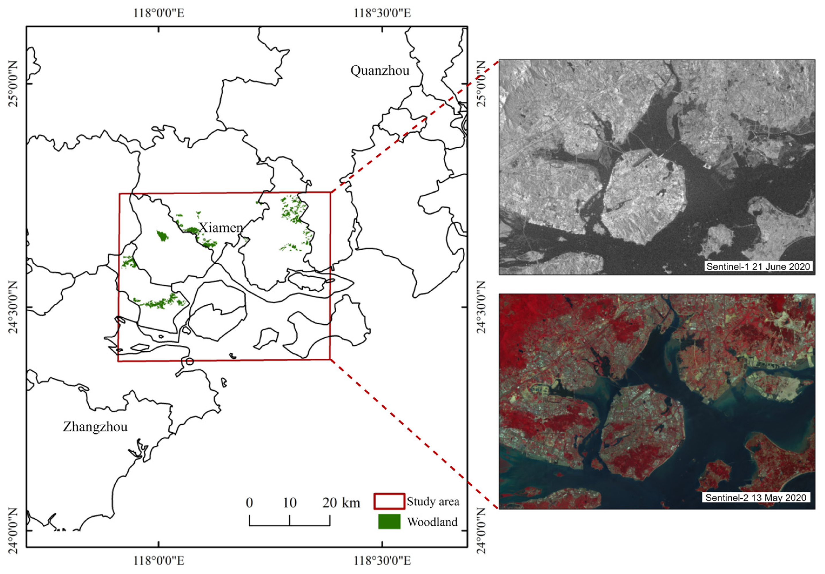
Xiamen is situated on the southeast coast of Fujian Province, between 24°26′46″ N and 118°04′04″ E (Figure 1). It comprises Xiamen Island, Gulangyu Island, and adjacent areas, with a total land area of 1700.61 km² and a sea area of approximately 390 km² [26]. The topography is characterized by hills, terraces, and coastal plains, sloping from northwest to southeast. The northwestern region features low-to-medium mountains, with the highest peak, Yunding Mountain, located at the border of Tong’an District and Anxi, reaching an elevation of 1175.2 m.

Xiamen has a southern subtropical maritime monsoon climate, with an annual average temperature of 20.9 °C and annual precipitation of about 1200 mm. The year can be divided into the spring rainy season (March–April), the plum rain season (May–June), the typhoon season (July–September), the autumn season (October–November), and the winter season (December–February) [27].

The zonal vegetation in Xiamen is a subtropical monsoon evergreen broadleaf forest. Due to historical vegetation loss, the current vegetation mainly consists of plantation forests, secondary forests, and scrubland. Broadleaf forests are mostly distributed on hills and terraces below 200 m elevation and are limited in area. Coniferous forests grow primarily in mountainous regions between 500 and 900 m elevation and are usually monoculture plantations [28]. Mixed forests occur in some areas below 500 m, while saline vegetation such as Mangrove is found on coastal mudflats. Aquatic vegetation is distributed in water bodies such as reservoirs and ponds.

2.2. Data Sources and Preprocessing

Dual-polarization Sentinel-1A SAR single look complex (SLC) data in IW mode (VV and VH) were acquired for 2020–2021, comprising 28 scenes (

Table 1. Selected Sentinel-1 remote sensing image parameters.

No.	Imaging Date	No.	Imaging Date	No.	Imaging Date	No.	Imaging Date	No.	Imaging Date
1	11 January 2021	7	11 May 2021	13	15 July 2020	19	8 September 2021	25	31 October 2020
2	16 February 2021	8	16 June 2021	14	3 August 2021	20	13 September 2020	26	12 November 2020
3	28 February 2021	9	21 June 2020	15	15 August 2021	21	2 October 2021	27	18 December 2020
4	12 March 2021	10	28 June 2021	16	20 August 2020	22	14 October 2021	28	30 December 2020
5	17 April 2021	11	3 July 2020	17	27 August 2021	23	19 October 2020
6	29 April 2021	12	10 July 2021	18	1 September 2020	24	26 October 2021

) [29]. Sentinel-2 optical imagery (Level-1C) was collected to characterize seasonal spectral dynamics; due to persistent cloud contamination in the study area, the Sentinel-2 time series was constructed primarily from 2020–2021 observations and supplemented with scenes from adjacent years when cloud-free observations were unavailable for key phenological windows (

Table 2. Selected Sentinel-2 remote sensing image parameters.

No.	Imaging Date	No.	Imaging Date	No.	Imaging Date	No.	Imaging Date	No.	Imaging Date
1	14 January 2018	7	5 March 2018	13	28 May 2021	19	17 August 2019	25	15 November 2019
2	29 January 2019	8	24 March 2020	14	2 June 2020	20	6 September 2019	26	30 November 2018
3	7 February 2021	9	4 April 2018	15	12 June 2020	21	10 October 2020	27	15 December 2019
4	13 February 2018	10	13 April 2020	16	22 July 2020	22	16 October 2019	28	20 December 2018
5	17 February 2021	11	3 May 2020	17	27 July 2021	23	21 October 2018	29	29 December 2020
6	23 February 2020	12	13 May 2020	18	7 August 2017	24	9 November 2020

(Note: Cloud-contaminated Sentinel-2 scenes were excluded; to fill key phenological windows, additional cloud-free scenes from adjacent years (2017–2019) were used to supplement the 2020–2021 time series.).

) [30]. This strategy was adopted to ensure continuity of the annual growth-cycle curves while minimizing temporal gaps caused by clouds.

Sentinel-1A data were processed in ESA SNAP, including precise orbit correction, radiometric calibration, multi-looking, speckle/polarimetric filtering, and terrain correction to generate terrain-corrected backscatter products. Sentinel-2 Level-1C images were processed using Sen2Cor, including radiometric and atmospheric correction, cloud screening, mosaicking/clipping, and resampling. To ensure pixel-wise comparability for multi-source feature extraction and fusion, both Sentinel-1 and Sentinel-2 products were resampled to a common spatial resolution of 20 m and co-registered to the same map projection before subsequent analysis.

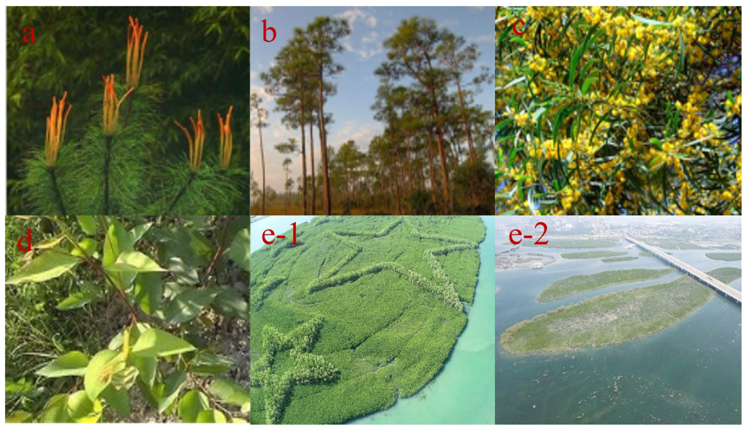
Based on forest inventory data from 2006 and the China Plant Image Library, the spatial distribution and climatic characteristics of typical tree species in the study area were obtained (

Table 3. Spatial distribution characteristics of tree species and phenological characteristics in the study area.

Tree Species	Spatial Distribution Characteristics	Climatic Information
		Flowering Period, Spike Stage	Characteristics of Tree Shape
Pinus massoniana	Widely distributed, it is the main tree species in the study area, mainly concentrated in Haicang District, Xiamen.	Flowering in April–May, fruit ripening in October–December of the following year.	Height up to 45 m, diameter at breast height 1.5 m; branches spreading or obliquely spreading, crown broadly tower-shaped or umbrella-shaped.
Pinus elliottii	Widely distributed, mainly located in the middle and southern part of Haicang District.	Flowering in summer, fruiting for one year	Height up to 30 m, diameter at breast height 90 cm; scale leaves are needle-shaped, seeds ovoid.
Acacia	Covering a large area, mainly in the central part of Haicang District, with a small distribution in Xiamen Island.	Flowering period from March to October; Fruiting period is from August to December	6–15 m tall; pinnately compound leaves in the seedling stage, with weak pedicels and ellipsoid seeds.
Eucalyptus grandis	Scattered distribution, mainly concentrated in some areas in the central part of Haicang District.	Flowerless, fruitless	Diameter at breast height up to 25 cm; species with elliptic leaves, 5–8 cm long, with sharp tips
Mangroves	Grows in the coastal intertidal zone, mainly distributed in Xiang’an District, and Tong’an District also has a small range of distribution	Flowering period is usually in spring and summer, and the fruiting period is in July–October.	Height varies, up to 30 m, with a well-developed root system.

), providing auxiliary data for subsequent tree species classification. To further improve the identification accuracy of typical tree species, three field surveys were conducted between December 2021 and December 2022, including ground photography and UAV aerial photography, to collect auxiliary information such as locations and distribution patterns of major tree species (Figure 2).

2.3. Research Methodology

2.3.1. Overall Workflow

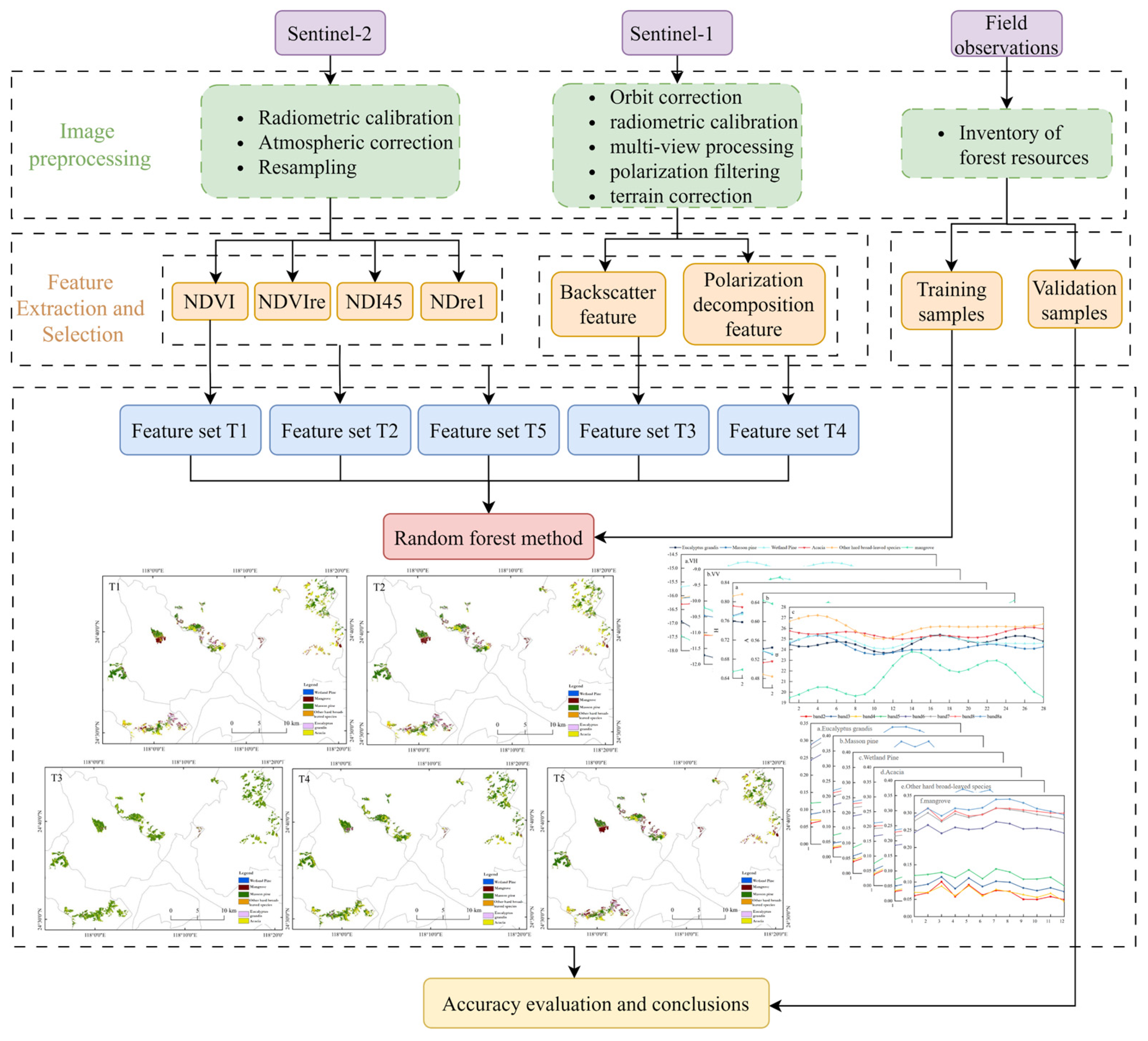
Addressing the challenge of tree species identification in subtropical cloudy and rainy regions, this study integrated Sentinel-2 optical images and Sentinel-1 SAR polarimetric data to construct a multi-source time-series remote sensing feature system. Multi-temporal vegetation indices and polarimetric scattering parameters were extracted. Based on the climatic traits and structural differences in typical tree species, five feature combination schemes were designed and used to train classification models. The Random Forest algorithm was then employed to identify six typical subtropical tree species. The overall accuracy, Kappa coefficient, producer accuracy, and user accuracy were calculated from the confusion matrix to systematically evaluate and compare the classification performance of each feature combination. The technical workflow is shown in Figure 3.

The five schemes were designed to progressively incorporate (i) optical spectral/vegetation-index information, (ii) SAR backscatter features, and (iii) polarimetric decomposition descriptors, thereby isolating the incremental benefits of each feature group under cloud-induced optical gaps.

2.3.2. Vegetation Index Extraction from Optical Remote Sensing Imagery

Vegetation indices (VIs) derived from optical imagery are widely used to characterize canopy greenness and vegetation vigor. Among them, the normalized difference vegetation index (NDVI) is a commonly adopted indicator related to canopy cover and vegetation status [31,32]. However, NDVI can saturate in dense subtropical forests with high leaf area and canopy closure, which may limit its sensitivity to subtle inter-species differences. To better capture phenological and biochemical variability, we therefore employed NDVI together with three red-edge-based indices: NDVIre, NDI45, and NDre1, which leverage Sentinel-2 red-edge reflectance that is responsive to changes across growth stages [33]. The definitions of the four indices are provided in

Table 4. Vegetation index.

Index	Equation	Reference
Normalized difference vegetation index (NDVI)	$\mathrm{NDVI}={\displaystyle \frac{{\rho }_4-{\rho }_3}{{\rho }_4+{\rho }_3}}$	Becker and Choudhury, 1988 [34]
Red Edge Normalized Vegetation Index (NDVIre)	$\mathrm{NDVIre}={\displaystyle \frac{{\rho }_8-{\rho }_5}{{\rho }_8+{\rho }_5}}$	Amaro et al., 2025 [35]
Red edge-red wave normalized vegetation index (NDI45)	$\mathrm{NDI}45={\displaystyle \frac{{\rho }_5-{\rho }_4}{{\rho }_5+{\rho }_4}}$	David et al., 2022 [36]
Normalized Red Edge Index (NDre1)	$\mathrm{NDre}1={\displaystyle \frac{{\rho }_6-{\rho }_5}{{\rho }_6+{\rho }_5}}$	Shirkey et al., 2022 [37]

Note: ${\rho }_4$ and ${\rho }_3$ are the surface reflectance in NIR and red band, ${\rho }_4$ is the visible red band reflectance, ${\rho }_5$ is the Red Edge 1 reflectance, ${\rho }_6$ is the Red Edge 2 reflectance, and ${\rho }_8$ is the NIR reflectance.

.

2.3.3. Polarimetric Scattering Feature Extraction from SAR Data

SAR-derived features were extracted to characterize canopy structural properties that are complementary to optical spectral and phenological information. Specifically, we derived two groups of SAR features: (i) dual-polarization backscattering coefficients (VV and VH) and (ii) polarimetric decomposition parameters, including scattering entropy (H), mean scattering angle ($\overline{\alpha }$), and anisotropy (A). The backscattering coefficients backscatter provides sensitivity to canopy structure and moisture conditions, whereas the decomposition parameters describe scattering behavior: H describes the randomness of the scattering mechanism and is suitable for characterizing mixed-scattering stand types, $\overline{\alpha }$ helps identify the dominant scattering type, especially in distinguishing between volume scattering and surface/double-bounce scattering; A characterizes the relative importance of secondary scattering contributions. The definitions and equations of these SAR features are summarized in

Table 5. Calculation formulae for SAR polarization features.

Characteristic Type	Indicator Name	Calculation Formula	Description
Backscattering Characteristics	Backscattering coefficient	${\sigma }^0\left(\mathit{dB}\right)=10\mathit{lgDN}$	${\sigma }^0$ is the value of the processed backscattering coefficient, DN is the pixel brightness, and dB is the intensity unit [38]
Polarization decomposition parameters	Scattering entropy (H)	$H=-P_1{\mathit{log}}_2{P}_1-P_2{\mathit{log}}_2{P}_2$, $0\le P={\displaystyle \frac{{\lambda }_i}{{\displaystyle {\sum }_{i=1}^2}{\lambda }_i}}\le 1$	$P_i$: pseudo-probability calculated based on the eigenvalues of the covariance matrix ${\lambda }_i$, reflecting the uncertainty of the scattering mechanism [38]
	Anisotropy degree (A)	$A={\displaystyle \frac{{\lambda }_1-{\lambda }_2}{{\lambda }_1+{\lambda }_2}}$, $0\le A\le 1$	Characterizes the degree of dominance of the scattering mechanism, when ${\lambda }_1$ ≈ ${\lambda }_2$, A is close to 1 and the scattering mechanism is single [39]
	Average scattering angle ($\overline{\alpha }$)	$\overline{\alpha }=P_1{\alpha }_1+P_2{\alpha }_2$, $\alpha \in [0,90]$	The larger the mean scattering angle, the more significant the body scattering, and vice versa, the surface scattering is dominant

.

2.3.4. Random Forest Algorithm

Random Forest (RF) is an ensemble learning method that constructs a large number of decision trees and combines their outputs through majority voting for classification [40]. RF is well suited to high-dimensional, heterogeneous remote sensing features because it does not require distributional assumptions and is relatively robust to multicollinearity and noise. In RF, each tree is trained using bootstrap sampling of the training data, and at each node a random subset of features is considered to determine the best split, which reduces inter-tree correlation and improves generalization [41].

In this study, RF was selected for three main reasons. The classification task involves multi-temporal Sentinel-2 optical indices and Sentinel-1 SAR-derived features, resulting in a high-dimensional feature space. RF has demonstrated strong capability in handling such data without extensive feature normalization or parameter tuning; RF provides intrinsic robustness to noise and outliers, which is particularly important in subtropical regions characterized by complex land-cover composition and spectral heterogeneity; RF offers internal measures of feature importance, facilitating the evaluation of the relative contributions of optical and SAR features under different feature combination strategies.

To further interpret the model behavior, SHAP [40] (SHapley Additive exPlanations) was applied as a post hoc explanation method. SHAP quantifies the contribution of each feature to the model predictions based on cooperative game theory, enabling consistent and comparable evaluation of feature effects across different feature schemes. This helps reveal how optical vegetation indices and SAR-derived structural parameters jointly influence tree species discrimination [41].

The RF model was implemented in Python. The number of trees was set to 550, and the maximum number of features considered at each split was defined as the square root of the total number of input features. All other parameters followed the default settings unless otherwise specified. Python is available at https://www.python.org/ (accessed on 2 November 2025).

2.3.5. Classification Sample Selection and Accuracy Evaluation

Based on Xiamen forest inventory data and high-spatial-resolution remote sensing images, sample points were selected for typical tree species, including 874 Eucalyptus grandis, 2637 Pinus massoniana, 932 Pinus elliottii, 1983 Acacia, 691 Mangrove, and 590 Other hardwoods. 70% of the samples were randomly selected for training, and 30% were used for validation.

Overall accuracy (OA), Kappa coefficient, producer accuracy (PA), and user accuracy (UA) were calculated from the confusion matrix to evaluate the classification performance of different feature combinations and identify the optimal classification strategy [42].

2.3.6. Feature Selection Criteria and Redundancy Control

To reduce feature redundancy and improve model robustness, feature selection was conducted by jointly considering temporal variability and inter-feature correlation. First, candidate features were examined across the time series, and variables showing pronounced temporal dynamics and clear class separability during key phenological stages were prioritized for retention. Second, Pearson correlation analysis was used to quantify redundancy among features. If the absolute correlation coefficient between two features was |r| > 0.80, the pair was treated as highly redundant and only one feature was retained—specifically, the variable exhibiting stronger temporal variability or better class discrimination. If |r| < 0.70, features were considered complementary and were preserved. For intermediate correlations (0.70 ≤ |r| ≤ 0.80), the decision was made based on comparative discriminatory performance.

From a conceptual perspective, redundancy in multi-temporal remote sensing features mainly arises when multiple variables capture similar phenological or structural responses at the same temporal stage [43]. By explicitly incorporating temporal variability into the selection process, the proposed strategy prioritizes features that represent distinct phenological phases where interspecies separability is maximized [44]. Correlation analysis further ensures that features conveying highly overlapping information within the same temporal window are not simultaneously retained. As a result, the joint consideration of temporal differences and inter-feature correlation effectively avoids repeated encoding of similar ecological signals, thereby reducing feature redundancy while preserving discriminative information [45].

3. Results and Analysis

3.1. Characterization of Optical Remote Sensing Features of Typical Tree Species

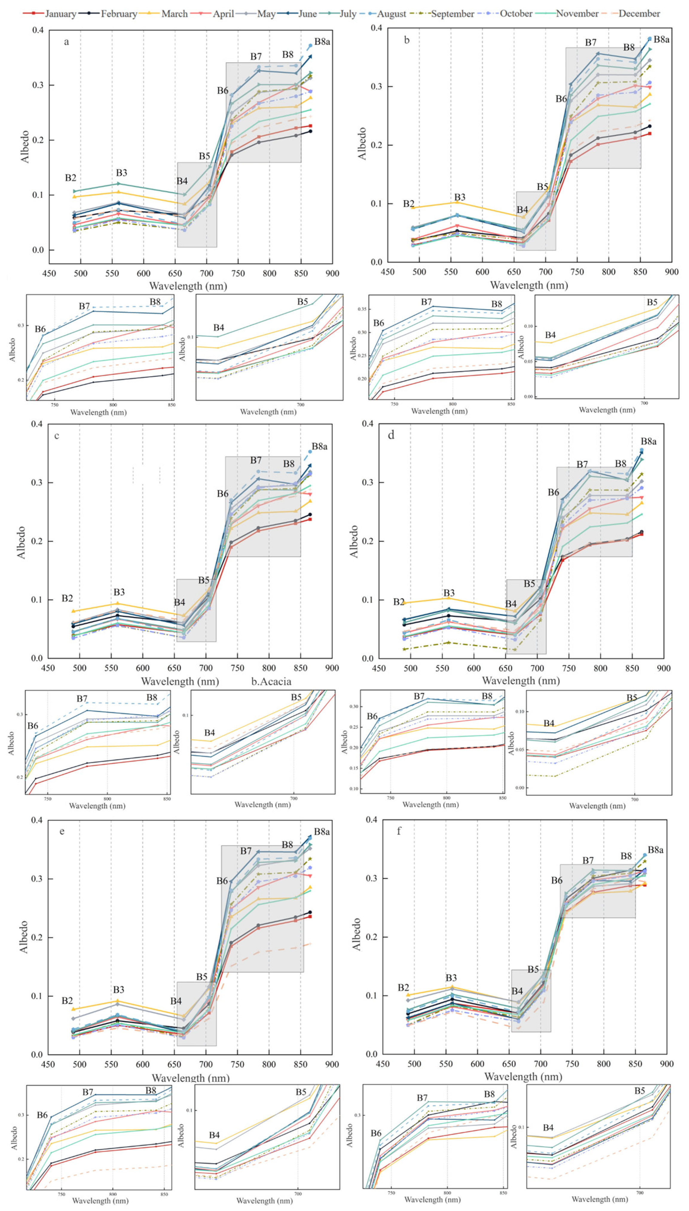
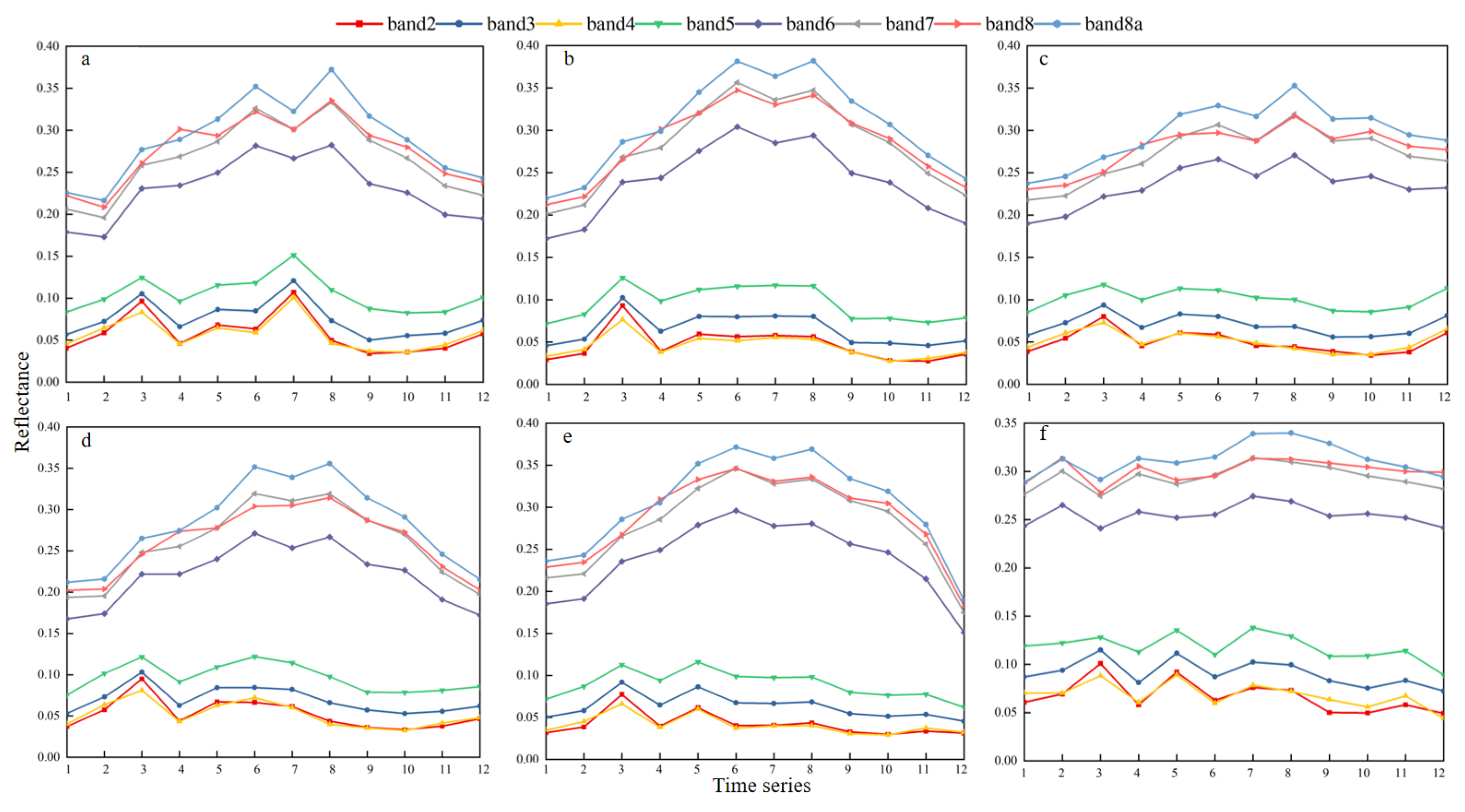
Different tree species exhibit variability in spectral reflectance. Figure 4 shows the spectral curves of six typical tree species from January to December. The spectral reflectance of the tree species ranges between 0.03 and 0.4. Changes in spectral reflectance in the visible bands (B2–B4) and the red-edge band (B5) are relatively small across months. However, reflectance increases rapidly in the red-edge band (B5) and gradually rises with increasing wavelength. Eucalyptus grandis, Pinus massoniana, Pinus elliottii, Acacia, and Other hardwoods reached the highest spectral reflectance from June to August, showing a strong spectral response during the growth period. From November to February of the following year, they entered a defoliation and withering stage, and reflectance in the near-infrared bands (B6–B8A) decreased, reaching the lowest values in winter, demonstrating seasonal variation characteristics. In contrast, Mangrove forests showed high stability throughout the year, with slightly higher reflectance in July and August but overall small fluctuations, reflecting their evergreen nature and intertidal distribution characteristics.

To further quantify the spectral response patterns of each tree species, the intra-annual time-series curves of spectral reflectance are shown in Figure 5. The results indicate that the spectral reflectance of all tree species in the visible bands (B2–B4) and the red-edge band (B5) is lower than that in the near-infrared bands (B6–B8), and the annual fluctuation of the former is generally smaller than that of the latter. Specifically, for reflectance in bands B2–B5, the peaks for Pinus massoniana, Pinus elliottii, Acacia, and Other hardwoods occurred in March; Eucalyptus grandis peaked in March and July; and Mangrove forests peaked in March, May, and July. For reflectance in bands B6–B8, except for Mangrove forests, all other tree species gradually increased from January, peaked in June, showed a decrease in July, declined further in August, and dropped rapidly after October, demonstrating a clear phenology-driven pattern. Reflectance of Mangrove forests in bands B6-B8A fluctuated minimally throughout the year, indicating better spectral stability compared to other forest types. This difference highlights the remote sensing characteristics of Mangrove forests, which exhibit perennial stable photosynthesis and occupy special ecological niches (e.g., patchy distribution in intertidal zones).

Overall, the above results demonstrate that different tree species exhibit distinct spectral reflectance levels and intra-annual variation patterns, particularly in the red-edge and near-infrared bands. These phenology-driven differences and species-specific stability characteristics provide a solid spectral basis for subsequent feature construction and multi-temporal analysis, and justify the use of time-series optical features in the following classification and feature fusion experiments.

3.2. Analysis of Polarimetric Scattering Characteristics of Typical Tree Species

3.2.1. Backscattering Characteristics of Typical Tree Species

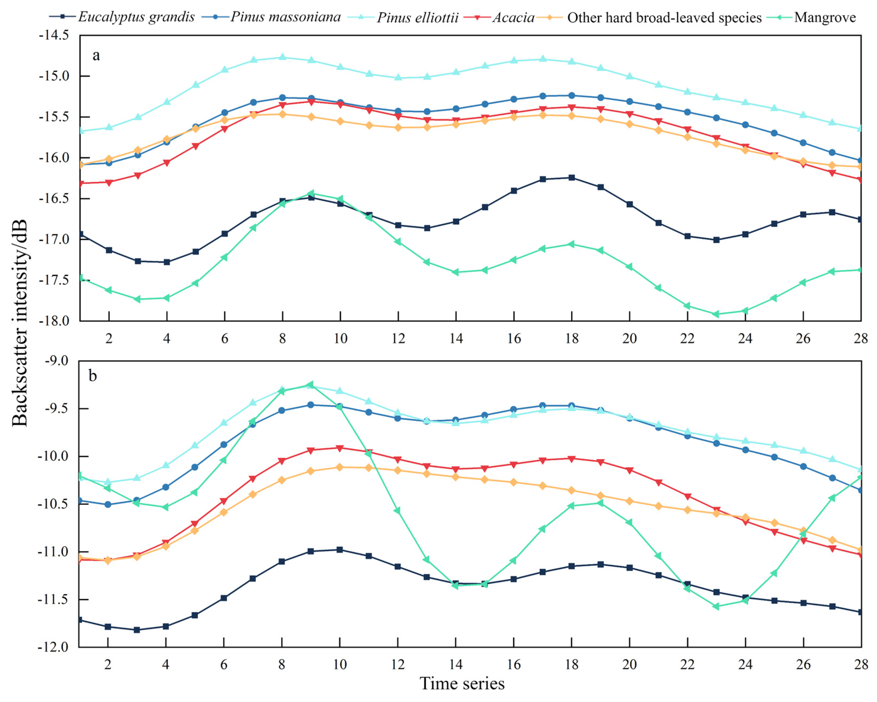
Figure 6 shows the one-year temporal dynamics of Sentinel-1 backscatter for the six tree classes under VH and VV polarizations. Overall, both polarizations exhibit class-dependent scattering levels and seasonal variability, indicating that SAR backscatter provides complementary structural information for tree species discrimination.

To clarify species-specific scattering behavior under different polarization modes, the VH polarization characteristics are first analyzed. As shown in Figure 6a, under VH polarization, the six tree species can be divided into three main groups based on scattering intensity: Pinus elliottii has significantly higher scattering coefficients than the other species, with smooth curve fluctuations, reflecting its compact structure and enhanced volume scattering; Pinus massoniana, Acacia, and Other hardwoods have similar scattering coefficients, ranging from −16.3 to −14.3 dB, with consistent curve trends and insignificant fluctuations; Eucalyptus grandis is lower, between −17.3 and −16.3 dB, with large fluctuations, indicating weak scattering response due to its loose canopy structure; Mangrove forests are the lowest, between −17.9 and −16.5 dB, with sharp curve fluctuations due to tidal disturbances. Seasonal changes show that Pinus elliottii, Pinus massoniana, Acacia, and Other hardwoods have similar curve shapes and consistent fluctuations. Their scattering coefficients gradually increased from January to June (points 1–8), with a notable increase after April (point 5), indicating entry into a rapid growth period and denser morphological structures. After late October (point 23), they entered a defoliation period, and the VH scattering coefficients decreased significantly. The VH scattering coefficient of Eucalyptus grandis remained low throughout the year (only higher than that of Mangrove forests), with large fluctuations, attributed to its sparse structure and sensitive growing environment. Mangrove forests had the lowest VH polarized backscattering intensity (with exceptions in a few months) and a significant range of fluctuations, related to their unique growing environment: partially submerged during high tide, showing characteristics of water/smooth mudflats, and with outer-edge silt during low tide, reducing scattering intensity.

In contrast to VH polarization, VV polarization is more sensitive to surface and canopy structure, and thus exhibits different inter-species separability. As shown in Figure 6b, under VV polarization, unlike VH, the six tree species can be divided into four main groups based on scattering intensity: Pinus elliottii has the highest scattering coefficient, and the difference with Pinus massoniana is reduced, concentrated between −10.5 and −9.3 dB, with similar curve patterns, peaking in June and declining after entering the defoliation period, indicating close scattering characteristics; Acacia and Other hardwoods have the second-highest scattering intensity, distributed between −11.0 and −10.0 dB, with the former’s trend closer to that of coniferous species; Eucalyptus grandis is the lowest throughout the year, with relatively small fluctuations; notably, influenced by tides and silt, Mangrove forests show significant fluctuations in VV polarized scattering characteristics, with coefficients dropping sharply in August and October due to high tide levels, demonstrating typical tidal disturbance characteristics. Combined with seasonal fluctuations under VV polarization, the scattering coefficient curves of Pinus massoniana and Pinus elliottii are highly consistent, peaking in June; the reflectance of Acacia and Other hardwoods is lower, with smoother curve fluctuations; and Eucalyptus grandis shows small-amplitude fluctuations. Mangrove forests exhibit typical tidal disturbance characteristics under VV polarization, especially at points 14–15 (August) and 22–24 (October), where scattering coefficients drop sharply due to high tide levels.

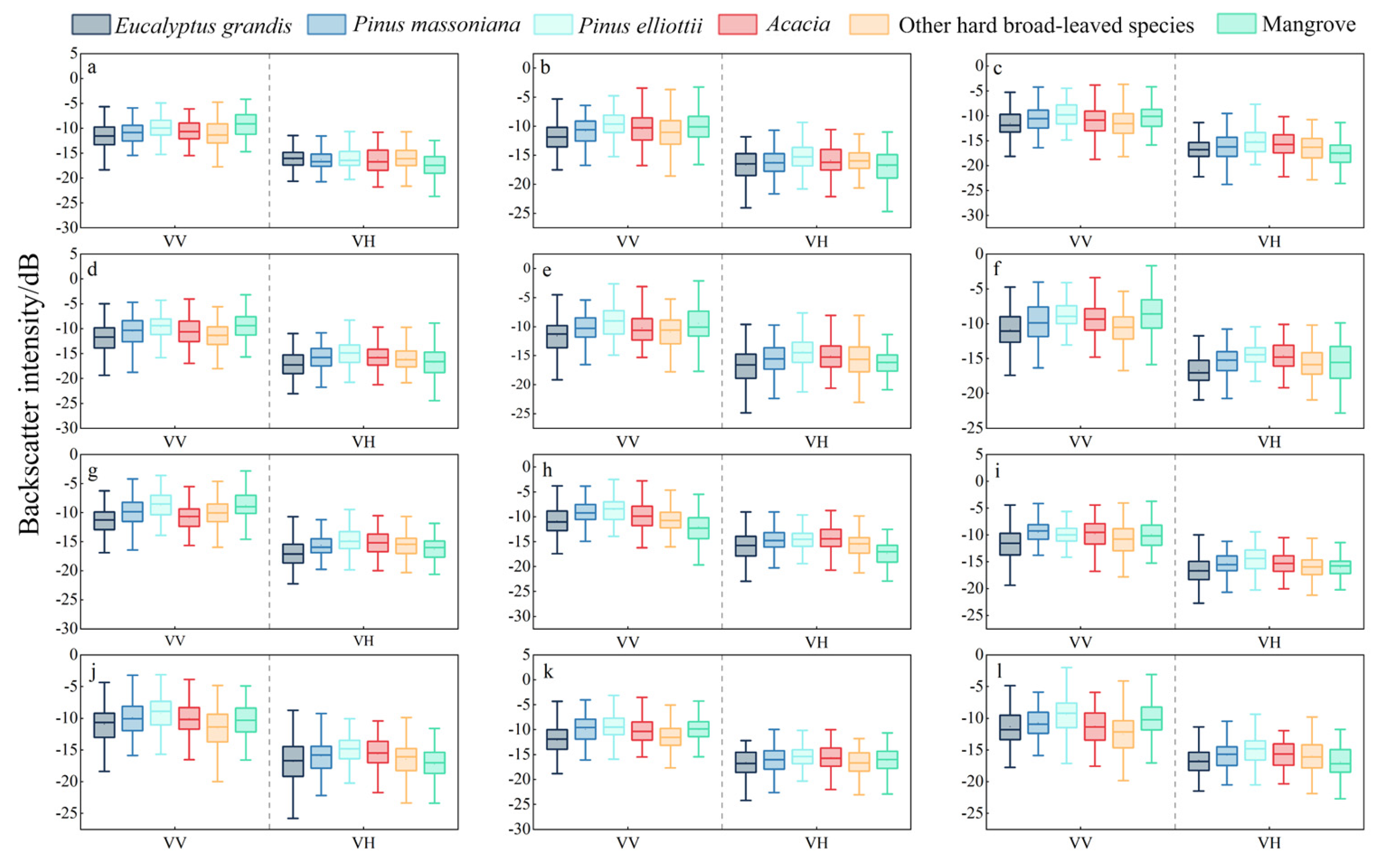
To further synthesize the polarization-dependent scattering differences, the monthly variation patterns under both VV and VH polarizations are summarized in Figure 7. Figure 7 shows the monthly trends in scattering intensity of typical tree species under VV and VH polarizations, reflecting good temporal variability and structural response characteristics. Under VV polarization, Pinus elliottii generally maintains higher VV backscatter with relatively compact dispersion across months, consistent with stable canopy structure. In contrast, Eucalyptus grandis shows large fluctuations in scattering coefficient and the lowest feature values in spring, clearly distinguishing it from other species; Mangrove forests, significantly affected by tidal cyclicity, show large differences from other species in January, June, and August, providing good discrimination advantages. In contrast, the scattering differences among Pinus massoniana, Acacia, and Other hardwoods are not significant, with limited ability for differentiation. Under VH polarization, the scattering coefficients of Mangrove and Eucalyptus grandis are relatively low throughout the year, with Mangrove forests particularly standing out in January, March, April, August, October, and December, showing high differentiation from other species; however, differences in scattering values among species narrow in winter, increasing the difficulty of differentiation.

Overall, both VV and VH polarizations provide key bases for identifying typical tree species, especially for species with significant structural characteristics such as Pinus elliottii, Eucalyptus grandis, and Mangrove forests. However, for species with similar structures, such as Pinus massoniana, Acacia, and Other hardwoods, it is still necessary to use other optical or polarimetric features to assist in differentiation and improve overall identification accuracy.

3.2.2. Analysis of Polarimetric Decomposition Characteristics of Typical Tree Species

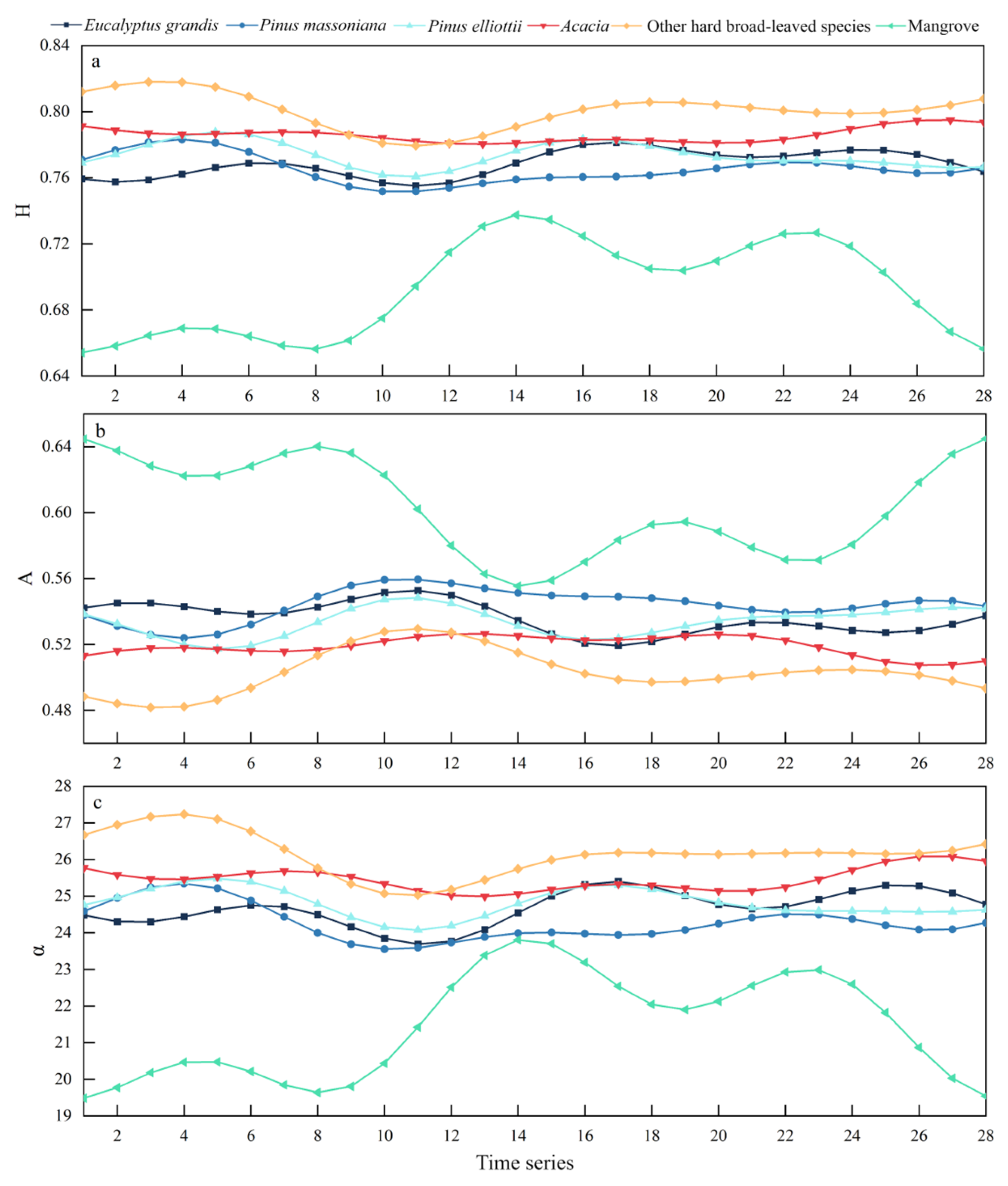
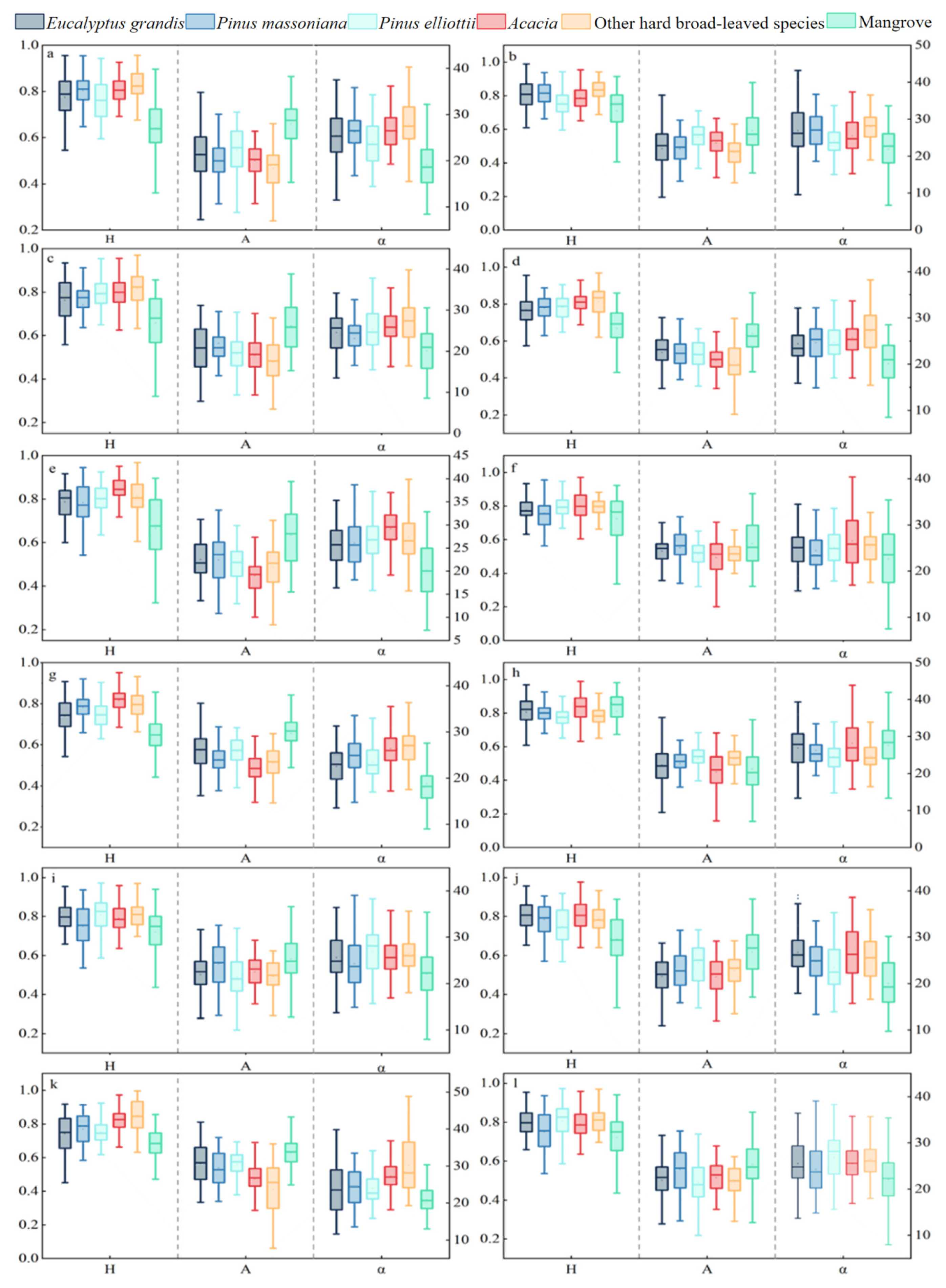
Figure 8 shows the time-series variation curves of polarimetric decomposition features for the six tree species. Mangrove forests exhibit significantly lower values in scattering entropy (H) and scattering angle ($\overline{\alpha }$) than other species, while showing higher values in anisotropy (A), indicating good separability. The values of scattering entropy (H) and scattering angle ($\overline{\alpha }$) for Acacia and Other hardwoods are higher than those of Eucalyptus grandis in most months, but the three species show similar anisotropy (A) to Pinus elliottii and Pinus massoniana, resulting in low differentiation. The scattering entropy (H) in Mangrove forest areas remains below 0.75, indicating relatively simple scattering types, while other species generally exceed 0.75, reflecting more complex scattering mechanisms. The anisotropy (A) values of Mangrove forests are above 0.56, whereas other species are below this value. In terms of scattering angle ($\overline{\alpha }$), Mangrove forests range between 20° and 24°, while other species are mainly distributed between 23° and 28°, indicating that surface scattering dominates in the areas covered by all tree species.

Monthly statistics are shown in Figure 9. The temporal performance of polarimetric decomposition features varies among tree species. Mangrove forests consistently exhibit lower scattering entropy (H) and mean scattering angle ($\overline{\alpha }$) than other species throughout the year, while maintaining the highest level of anisotropy (A), demonstrating significant distinguishability. From January to April, Other hardwoods show the lowest (A) values and relatively high ($\overline{\alpha }$) values, suggesting that their scattering mechanisms are dominated by random scattering during this period. In other months, the polarimetric characteristics of these species gradually converge with those of Acacia, showing strong similarity in the mid-to-late period. In contrast, the polarimetric feature values of Pinus massoniana, Pinus elliottii, and Eucalyptus grandis remain relatively close throughout the year, making it difficult to differentiate them effectively using polarimetric decomposition features.

In summary, polarimetric decomposition parameters are highly capable of distinguishing Mangrove forests but show limited effectiveness in differentiating other common forest types, particularly among structurally similar coniferous species. Therefore, relying solely on SAR polarimetric decomposition information is insufficient for precise tree species identification. There is an urgent need to integrate spectral features, temporal variation patterns, and backscattering intensity from optical remote sensing imagery to enhance the distinguishability and classification accuracy of different tree species.

3.3. Typical Tree Species Remote Sensing Feature Correlation Analysis

3.3.1. Correlation Analysis of Vegetation Indices for Typical Tree Species

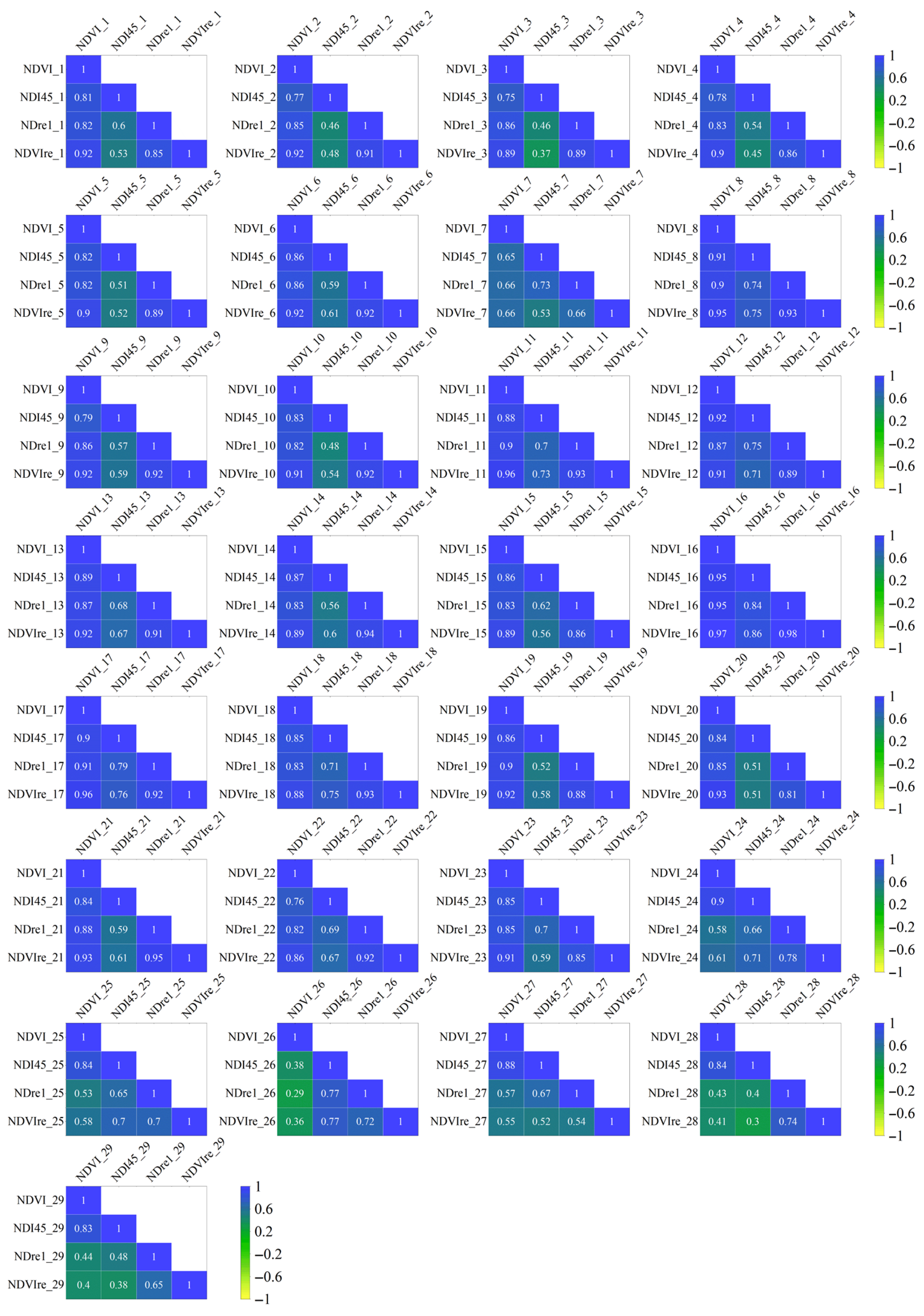
Vegetation indices derived from Sentinel-2 images exhibit strong correlations among some features, which can lead to data redundancy and the “curse of dimensionality,” thereby affecting classification accuracy and efficiency [46]. In this study, four vegetation indices were extracted from 29 Sentinel-2 images, generating 116 feature variables. To avoid redundant information, correlation analysis was performed on all features to construct a feature correlation matrix (Figure 10), revealing redundant structures among variables and assisting in feature selection.

Figure 10 illustrates the time-series correlations between NDVI and three red-edge indices (NDI45, NDVIre, and NDre1). Overall, the correlations show strong consistency while also revealing independent characteristics among some indices. Specifically, NDVI exhibits high correlation with NDVIre and NDre1, with Pearson coefficients mostly ranging between 0.82–0.97. However, during November-December (points 24–29), the correlation drops to 0.29–0.61. In contrast, the correlation between NDVI and NDI45 is relatively lower, generally ranging between 0.75–0.95, and dropping to 0.38 during specific periods (e.g., November point 26), indicating that NDI45 provides substantial information gain during certain time phases. Meanwhile, NDI45 shows moderate correlation (0.3–0.8) with NDVIre and NDre1, with obvious temporal variability. For example, correlation coefficients fluctuate between 0.37–0.65 in January-February, April, June, and September-October, while the correlation between NDI45 and NDVIre/NDre1 in March (point 7) is higher. The correlation between NDVIre and NDre1 is generally greater than 0.8 from January to October, but decreases significantly to as low as 0.54 in November-December (points 25–29). In summary, there is some redundancy among NDVI, NDVIre, and NDre1 in characterizing canopy leaf area, especially during rapid vegetation growth periods, where they show highly consistent phenological responses. In contrast, NDI45 is only moderately correlated with the other indices, possessing relatively independent information dimensions, making it suitable as an auxiliary feature to enhance the differential expression capability of tree species classification models.

Accordingly, VI variables showing |r| > 0.80 were screened following Section 2.3.6, retaining the more discriminative/red-edge-sensitive variables while keeping NDI45 as a complementary index to reduce redundancy.

3.3.2. Correlation Analysis of Polarized Scattering Features for Typical Tree Species

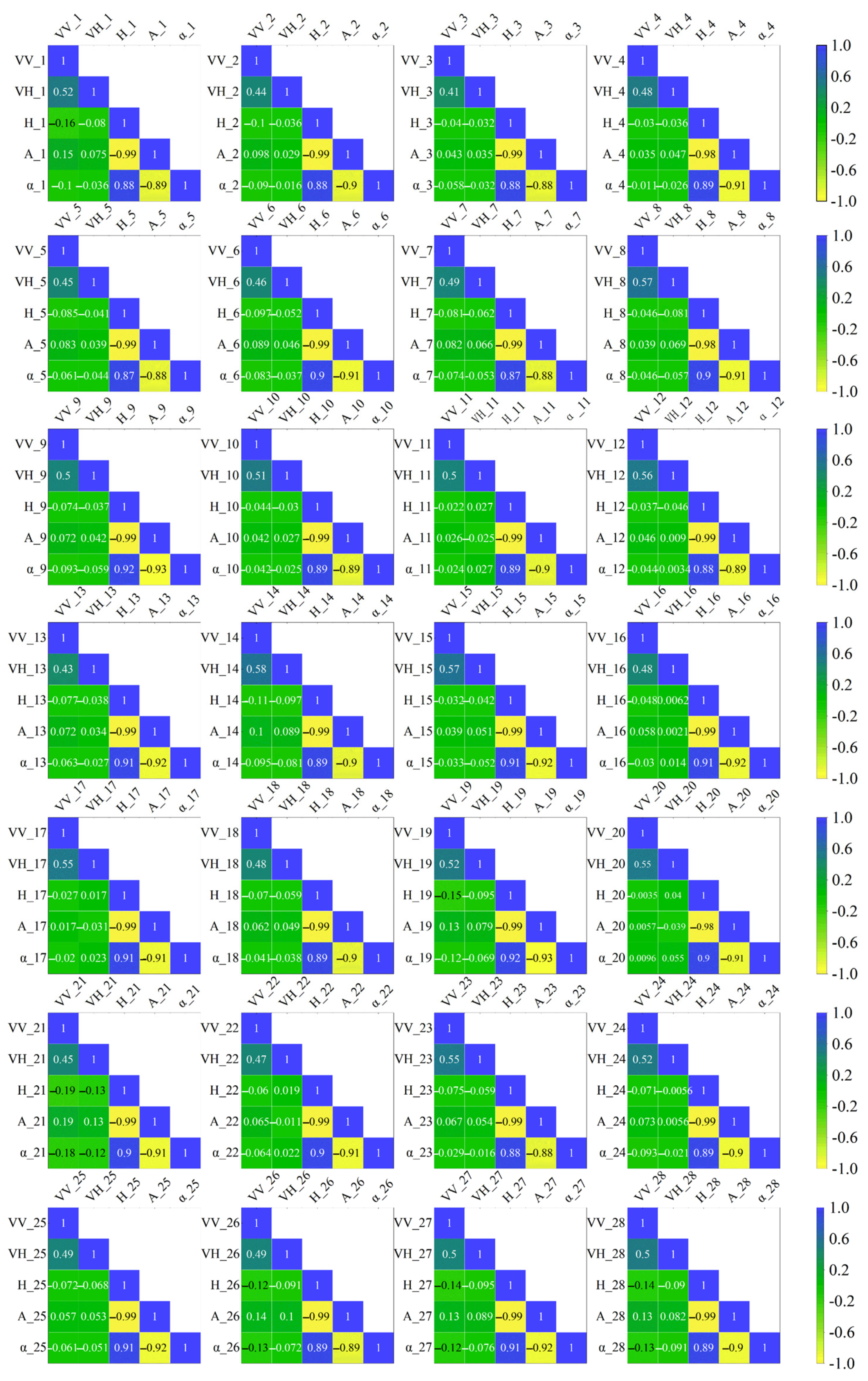
From the 28 Sentinel-1 acquisitions, we derived five SAR feature types-VV and VH backscatter coefficients and three polarimetric decomposition parameters (H, A, and $\overline{\alpha }$)-yielding 140 SAR-related variables in total. Figure 11 summarizes Pearson correlations among these features and provides evidence to guide redundancy control.

Overall, VV and VH polarized backscattering show moderate correlation, with correlation coefficients of approximately 0.4–0.6, indicating that the two are complementary in characterizing vegetation structure. The correlation coefficients between these two features and polarimetric scattering entropy (H) and scattering angle ($\overline{\alpha }$) range from −0.01 to −0.1, while those with anisotropy A range from 0.15 to 0.2, indicating that the scattering coefficients are relatively independent of the polarimetric decomposition parameters in terms of information dimension. Additionally, the correlations among polarimetric decomposition parameters are strong: the correlation coefficients between H and $\overline{\alpha }$ are all above 0.87, showing a strong positive correlation, reflecting their consistency in scattering mechanisms (e.g., the weights of volume scattering and surface scattering). The correlation coefficients between H, $\overline{\alpha }$, and A range from −0.88 to −0.99, indicating that the trend of anisotropy exhibits an inverse relationship with scattering entropy and mean scattering angle. In summary, for the six typical subtropical tree species, there are significant structural correlations among SAR polarization feature dimensions. The backscattering coefficients (VV, VH) and polarimetric decomposition parameters (H, $\overline{\alpha }$, A) have different information sources, are complementary, and are suitable for joint modelling. However, the polarimetric decomposition parameters are highly internally correlated, and the simultaneous introduction of multiple highly correlated parameters should be avoided.

Accordingly, when |r| exceeded 0.80 within the decomposition parameters (e.g., between H and $\overline{\alpha }$), only one variable was retained based on temporal variability and discriminatory performance.

3.4. Evaluation of Tree Classification Performance Under Different Feature Combinations

3.4.1. Classification Feature Construction and Combination Methods

To clarify the effects of different information sources and feature complexity on tree species classification performance, this study adopts a progressive comparison strategy of “single-source features—multi-feature expansion—multi-source fusion” at the feature construction stage. Based on time-series data from Sentinel-2 optical imagery and Sentinel-1 SAR imagery, multi-class vegetation indices and SAR polarimetric features were systematically analyzed in terms of their temporal variation characteristics and inter-variable correlations. Under the premise of maximizing feature separability while minimizing redundancy, five representative feature combination schemes (T1–T5) were constructed, covering optical vegetation indices, SAR backscattering features, and polarimetric decomposition parameters, and were subsequently used to train classification models and compare tree species classification performance under different feature configurations. Reference samples for each tree species were selected based on forest resource inventory data of Xiamen City and visual interpretation of high-resolution remote sensing imagery. All samples were randomly divided into a training set (70%) and a validation set (30%). During model training, bootstrap resampling was applied to the training samples to enhance model robustness and reduce potential sampling bias.

For optical remote sensing features, the time-series trends and correlation indices of four vegetation indices (NDVI, NDI45, NDVIre, and NDre1) were integrated to screen out highly discriminative features in key months: (1) During January–February, the NDVI and NDI45 values of Pinus massoniana and Other hardwoods were significantly higher than those of other species. The correlation between NDVI and NDVIre/NDre1 was higher than 0.8, while the correlation between NDI45 and NDVIre/NDre1 was lower than 0.6. NDVI_1-NDVI_6 and NDI45_1-NDI45_6 were retained (where the number indicates the remote sensing image identifier). (2) In March, the correlations among indices for point 7 are generally lower than 0.7, and the differences between variables are obvious; all features were retained. For point 8, NDI45 shows good differentiation, with a correlation coefficient above 0.9 against NDVI; thus, NDI45_8 was retained. (3) From April to May, the correlation between NDVI and NDI45 for point 9 is lower than 0.8, while their correlations with NDVIre and NDre1 exceed 0.85; thus, NDVI_9 and NDI45_9 were retained. For points 10–13, NDI45 varies significantly among species, with correlations with NDVIre and NDre1 ranging from 0.5 to 0.75; thus, NDI45_10 to NDI45_13 were retained. (4) In June, NDVI can better distinguish Pinus elliottii from other tree species; thus, NDVI_14 and NDVI_15 were retained. (5) From August to October, the NDVI of Mangrove forests (points 19–23) differs significantly from that of other tree species; thus, NDVI_19 to NDVI_23 were retained. (6) In November–December, the correlation between NDVI and NDVIre/NDre1 for points 26–29 is low (r = 0.2–0.6); thus, NDVI_26 to NDVI_29 were retained. The correlation between NDI45 and NDVI for points 27–29 exceeds 0.8, indicating high redundancy, so these were excluded. The correlation coefficients between NDVIre/NDre1 and NDI45/NDVI for points 24–29 range from 0.2 to 0.6; thus, all were retained. The results are shown in

Table 6. Sentinel-2 image classification feature filtering (NDVI_1 represents NDVI features extracted from Sentinel-2 acquisition indexed as 1 in Table 2, NDVI_2 represents NDVI features from Sentinel-2 data with date number 2, and so on).

Vegetation Index	Characteristic Variable
NDVI	NDVI_1, NDVI_2, NDVI_3, NDVI_4, NDVI_5, NDVI_6, NDVI_7, NDVI_9, NDVI_13, NDVI_14, NDVI_15, NDVI_19, NDVI_20, NDVI_21, NDVI_22, NDVI_23, NDVI_26, NDVI_27, NDVI_28, NDVI_29
NDI45	NDI45_1, NDI45_2, NDI45_3, NDI45_4, NDI45_5, NDI45_6, NDI45_7, NDI45_8, NDI45_9, NDI45_10, NDI45_11, NDI45_12, NDI45_13, NDI45_14, NDI45_15, NDI45_16, NDI45_17, NDI45_18, NDI45_19, NDI45_20, NDI45_21, NDI45_22, NDI45_23, NDI45_24, NDI45_25, NDI45_26
NDVIre	NDVIRE_7, NDVIRE_12, NDVIRE_24, NDVIRE_25, NDVIRE_26, NDVIRE_27, NDVIRE_28, NDVIRE_29
NDre1	NDRE1_7, NDRE1_24, NDRE1_25, NDRE1_26, NDRE1_27, NDRE1_28, NDRE1_29

.

Similarly, the polarized backscattering coefficient of VV throughout the year showed good separability between Pinus elliottii, Pinus massoniana, Acacia, Other hardwoods and Eucalyptus grandis, and Mangrove also showed significant differences from the other species in most months. The correlation of the polarized backscattering coefficient of VH with VV was low (r ≈ 0.5), and negatively correlated with the polarized scattering entropy (H), and the average scattering angle ($\overline{\alpha }$) (r ≈ −0.1), while it was positively correlated with the degree of anisotropy (A) was positively correlated (r ≈ 0.1), retaining the VV polarized backward scattering characteristics throughout the year. The VH polarization coefficient was highest in Pinus elliottii and lowest in Mangroves, with good overall differentiation. Its correlation with VV polarization was always low, weakly negatively correlated with A in some periods (e.g., July, September, October), and weakly positively correlated in the rest of the months; its correlation with H and $\overline{\alpha }$ was always low (−0.02 to −0.14), and it retained the backscattering characteristics of VH polarization throughout the year. As for the polarization decomposition parameters, the time-series trends of H, $\overline{\alpha }$ and A are highly consistent, and the positive correlation between H and $\overline{\alpha }$ is much greater than 0.8, while both are strongly negatively correlated with A (r ≈ −0.9) with a high degree of redundancy. As a results,

Table 7. Sentinel-1 image classification feature screening (numbers VV_1-VV_28 represent VV-polarized backscattering features of Sentinel-1 images numbered 1–28 in Table 1).

Feature Name	Feature Parameter
VV	VV_1, VV_2, VV_3, VV_4, VV_5, VV_6, VV_7, VV_8, VV_9, VV_10, VV_11, VV_12, VV_13, VV_14, VV_15, VV_16, VV_17, VV_18, VV_19, VV_20, VV_21, VV_22, VV_23, VV_24, VV_25, VV_26, VV_27, VV_28
VH	VH_1, VH_2, VH_3, VH_4, VH_5, VH_6, VH_7, VH_8, VH_9, VH_10, VH_11, VH_12, VH_13, VH_14, VH_15, VH_16, VH_17, VH_18, VH_19, VH_20, VH_21, VH_22, VH_23, VH_24, VH_25, VH_26, VH_27, VH_28
H	H_1, H_2, H_3, H_4, H_5, H_6, H_7, H_8, H_9, H_10
A	A_11, A_12, A_13, A_14, A_15, A_16, A_17, A_18, A_19, A_20
$\overline{\alpha }$	$\overline{\alpha }$$\text{\_}21,\overline{\alpha }$$\text{\_}22,\overline{\alpha }$$\text{\_}23,\overline{\alpha }$$\text{\_}24,\overline{\alpha }$$\text{\_}25,\overline{\alpha }$$\text{\_}26,\overline{\alpha }$$\text{\_}27,\overline{\alpha }\text{\_}28$

summarized the screened Sentinel-1 feature variables.

Based on this, five feature combination schemes (T1–T5) were constructed to explore the recognition accuracy of tree species in subtropical regions under different feature combinations (

Table 8. Feature combination scheme for tree species classification.

Feature Set	Feature Combination	Feature Description
T1	NDVI	NDVI(20)
T2	NDVI + red edge index	NDVI(20) + NDI45(26) + NDVIre(8) + NDre1(8)
T3	Backscattering characteristics	VV(28) + VH(28)
T4	Backscattering feature + Polarization decomposition feature	${\mathrm{VV}}^{\left(28\right)}+{\mathrm{VH}}^{\left(28\right)}+{\mathrm{H}}^{\left(10\right)}+{\mathrm{A}}^{\left(10\right)}+{\overline{\alpha }}^{\left(8\right)}$
T5	NDVI + red edge index + Backscattering features + Polarization decomposition features	${\mathrm{NDVI}}^{\left(20\right)}+{\mathrm{NDI}45}^{\left(26\right)}+{\mathrm{NDVIre}}^{\left(8\right)}+{\mathrm{NDre}1}^{\left(7\right)}+{\mathrm{VV}}^{\left(28\right)}+{\mathrm{VH}}^{\left(28\right)}+{\mathrm{H}}^{\left(10\right)}+{\mathrm{A}}^{\left(10\right)}+{\overline{\alpha }}^{\left(8\right)}$

Note: (20) in NDVI⁽²⁰⁾ denotes the number of dimensions of the NDVI vegetation index participating in the classification features, and so on, and the data corresponding to each dimension are detailed in Table 4 and Table 5.

): T1 contains only multi-temporal NDVI to assess the classification effect of a single vegetation index. T2 adds three time-series red-edge index features to T1 to assess the contribution of red-edge bands to tree species classification. T3 contains Sentinel-1’s VV and VH polarized backscattering coefficients to analyze the independent classification ability of SAR backscattering features. T4 adds scattering entropy (H), anisotropy (A), and mean scattering angle ($\overline{\alpha }$) to T3 to assess the enhancement of SAR classification performance by polarimetric features. T5 integrates feature information from Sentinel-1 and Sentinel-2 remote sensing images, combining vegetation indices with polarized scattering features to comprehensively evaluate their synergistic classification capability.

3.4.2. Comparative Analysis of Classification Results Based on Random Forests

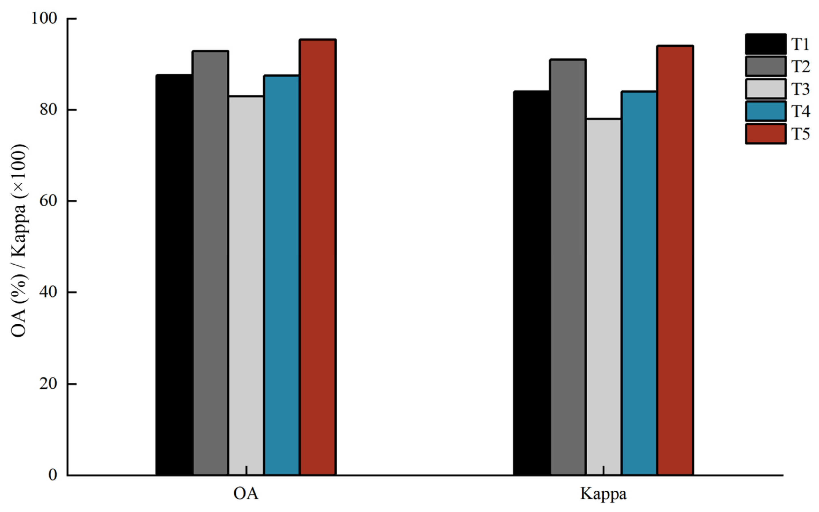
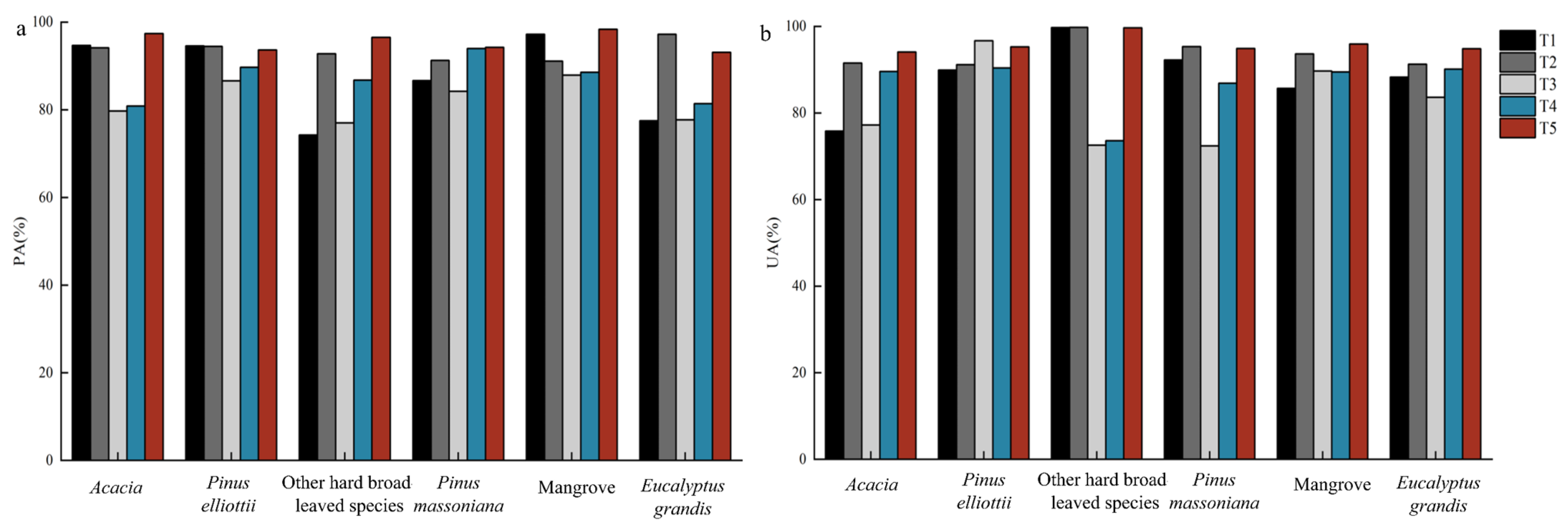
Using the five feature combination classification schemes, the Random Forest (RF) algorithm was applied to classify six typical subtropical tree species, including Eucalyptus grandis, Pinus elliottii, Pinus massoniana, Acacia, Mangrove, and Other hardwoods. The classification results were quantitatively evaluated using Overall Accuracy (OA), Kappa coefficient, Producer’s Accuracy (PA), and User’s Accuracy (UA) (

Table 9. Accuracy evaluation of classification results of each tree species using random forest for feature set T1–T5.

Tree Species Category	Accuracy Index	Acacia	Pinus elliottii	Other Hardwoods	Pinus massoniana	Mangrove	Eucalyptus grandis	OA	Kappa
T1	PA (%)	94.68	94.58	74.25	86.66	97.22	77.48	87.53	0.84
	UA (%)	75.83	89.90	99.69	92.22	85.71	88.27
T2	PA (%)	94.16	94.48	92.77	91.27	91.09	97.22	92.83	0.91
	UA (%)	91.55	91.18	99.78	95.31	93.66	91.24
T3	PA (%)	79.72	86.63	77	84.24	87.9	77.72	82.94	0.78
	UA (%)	77.22	96.70	72.6	72.43	89.71	83.63
T4	PA (%)	80.87	89.68	86.75	93.97	88.55	81.41	87.5	0.84
	UA (%)	89.61	90.41	73.6	86.86	89.46	90.11
T5	PA (%)	97.40	93.67	96.5	94.27	98.34	93.1	95.33	0.94
	UA (%)	94.06	95.27	99.67	94.91	95.95	94.85

, Figure 12 and Figure 13).

Figure 12 shows a clear performance hierarchy across feature schemes. The multi-source fusion scheme T5 achieves the highest overall performance (OA 95.33%, Kappa 0.94), followed by the red-edge-enhanced optical scheme T2 (OA 92.83%, Kappa 0.91). The optical baseline T1 and the SAR scheme with polarimetric descriptors T4 provide comparable overall accuracy (OA 87.53% and 87.50%, Kappa both 0.84), whereas the SAR backscatter-only scheme T3 performs worst (OA 82.94%, Kappa 0.78). These results indicate that introducing red-edge information substantially strengthens optical-only classification, and that the greatest gains are obtained when optical indices are fused with SAR backscatter and polarimetric features.

Class-wise accuracies in Figure 13 and Table 9 further clarify how different feature sources affect each tree class. Under T1, the main weakness is the reduced separability of hardwood-related classes, especially Other hardwoods (PA 74.25%), despite a high UA (99.69%), implying that omission errors dominate for this class. After incorporating red-edge indices (T2), class-wise performance improves markedly, with Other hardwoods showing a substantial PA gain (74.25% to 92.77%) while maintaining very high UA (99.78%). This improvement confirms that red-edge-sensitive indices contribute additional discriminative information beyond NDVI, particularly for classes with subtle spectral differences [47].

In comparison, SAR features alone show limited capability for separating several upland forest classes. Using VV/VH backscatter only (T3) yields lower and less stable class-wise reliability, with notably reduced UA for Pinus massoniana (72.43%) and Other hardwoods (72.60%), consistent with confusion among structurally similar canopies when relying solely on intensity features. Adding polarimetric decomposition parameters (T4) improves the SAR-only baseline (OA 82.94% to 87.50%), and increases classification reliability for some classes (e.g., Pinus massoniana PA 93.97%, Eucalyptus grandis UA 90.11%). However, Other hardwoods remains comparatively uncertain (UA 73.60%), indicating that SAR polarimetric descriptors alone are still insufficient to fully resolve broadleaf-related confusion.

The fusion scheme T5 provides the most consistent and accurate class-wise performance (Figure 13; Table 9). All classes exceed 93% in both PA and UA, with the highest PA observed for mangrove (98.34%). Relative to single-source schemes, T5 substantially reduces confusion among upland plantation and hardwood-related classes, demonstrating the complementary value of combining red-edge optical information with SAR backscatter and polarimetric scattering descriptors. Overall, these results validate that multi-source temporal feature fusion is critical for achieving robust, high-accuracy subtropical tree-species mapping under complex environmental conditions [48].

Additionally, Mangrove forests consistently achieved higher recognition accuracy across all feature combinations, primarily due to their typical ecophysiological characteristics (exposed root systems, intertidal patchy distribution, low mixing with other species), enabling distinct discriminative features in both optical and radar feature spaces [49].

3.4.3. Comparative Analysis of Spatial Performance and Accuracy of Classification Effect

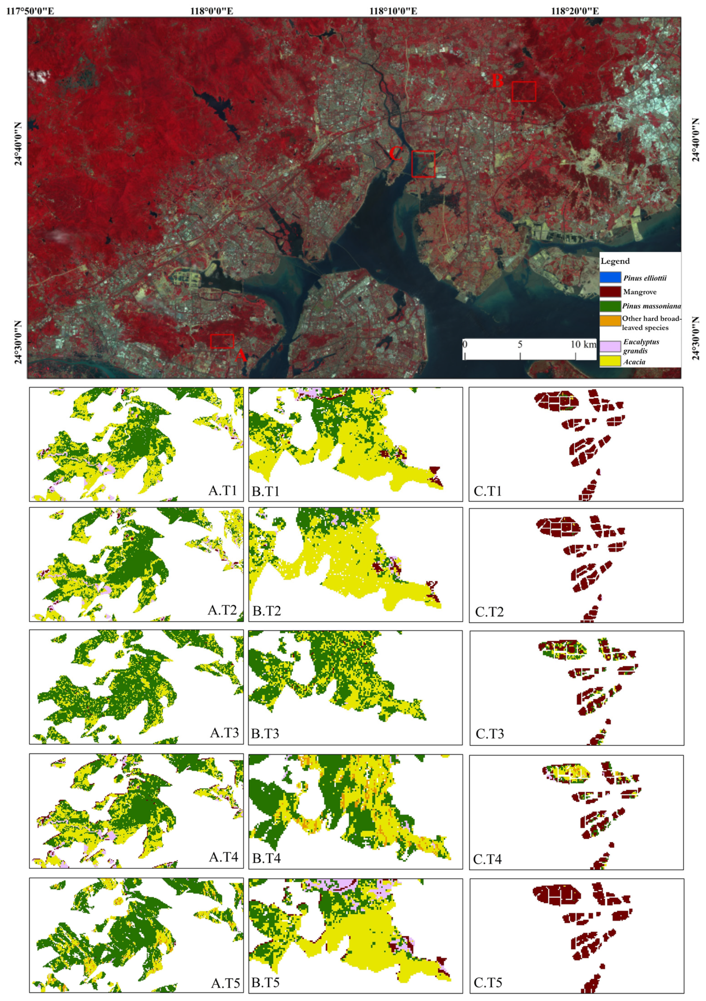
To further evaluate the spatial reliability and local consistency of tree-species mapping under different feature schemes, three representative subregions (A–C) were selected for zoomed-in comparisons (Figure 14). Region A represents an area where coniferous and broadleaf tree species coexist and exhibit similar spectral characteristics, resulting in pronounced classification confusion. Region B exhibits relatively continuous forest cover and lower background heterogeneity, providing a quasi-homogeneous setting to assess mapping stability and patch integrity. Region C represents a mangrove-dominated area with complex environmental conditions and strong ecological heterogeneity, serving as a representative case for assessing classification robustness in complex ecosystems.

Region A, located in the southwestern part of Xiamen City, is dominated by Pinus massoniana and Acacia and is prone to confusion due to their comparable spectral/structural responses. Using the NDVI-only scheme (T1), Pinus massoniana and Acacia are strongly mixed, and Acacia appears as fragmented patches, indicating limited spatial coherence. Incorporating SAR polarimetric decomposition parameters (T4) partially improves boundary delineation of Pinus massoniana stands and reduces salt-and-pepper noise, yet residual confusion with Acacia remains. The fused scheme (T5) provides the most coherent spatial patterns, substantially improving patch integrity of Pinus massoniana and reducing misclassification with Acacia, consistent with its superior class-wise performance.

Region B is located in the northeast and is primarily composed of Pinus massoniana and Acacia but features a more continuous forest distribution. Under T1, the overall structure of Acacia patches was complete, but some pixels were misclassified as Pinus massoniana, and a small number were misclassified as Mangrove forests and Eucalyptus grandis. T2 improved the confusion between Pinus massoniana and Acacia, and the internal areas of Acacia patches were more complete compared to T1, though a small number were still classified as Mangrove forests and Eucalyptus grandis. T3 exhibited weaker recognition capability, with large areas of Acacia misclassified as Pinus massoniana. T4 reduced the confusion between Pinus massoniana and Acacia after incorporating polarimetric features, though some misclassification as Other hardwoods persisted. T5 achieved the highest classification accuracy, with complete internal areas of Acacia patches, fewer finely fragmented patches, and significantly reduced misclassification with Pinus massoniana.

Region C is located in the Xiamen Xiang’an Mangrove Wetland Park, which is predominantly Mangrove forests and represents a heterogeneous intertidal environment. The optical-only schemes (T1 and T2) largely preserve the internal integrity of mangrove patches, with only limited confusion with nearby upland classes such as Pinus massoniana and Acacia. In contrast, the SAR backscatter-only scheme (T3) produces more fragmented mangrove patterns and increased mixing with Pinus massoniana/Acacia, indicating that intensity-based SAR features alone are insufficient to maintain spatial coherence in complex coastal settings. After adding polarimetric decomposition parameters (T4), local consistency improves in some areas but notable confusion persists, including overestimation of mangrove within Acacia-dominated patches and sporadic misclassification within mangrove stands. The fused scheme (T5) yields the most reliable spatial mapping, maintaining coherent mangrove interiors and providing clearer separation from surrounding tree classes.

Overall, the local comparisons across Regions A–C confirm that T5 improves not only quantitative accuracy but also spatial coherence, yielding more contiguous patches and fewer salt-and-pepper artifacts than single-source schemes.

3.4.4. Feature Importance Analysis Under Different Feature Combination Schemes

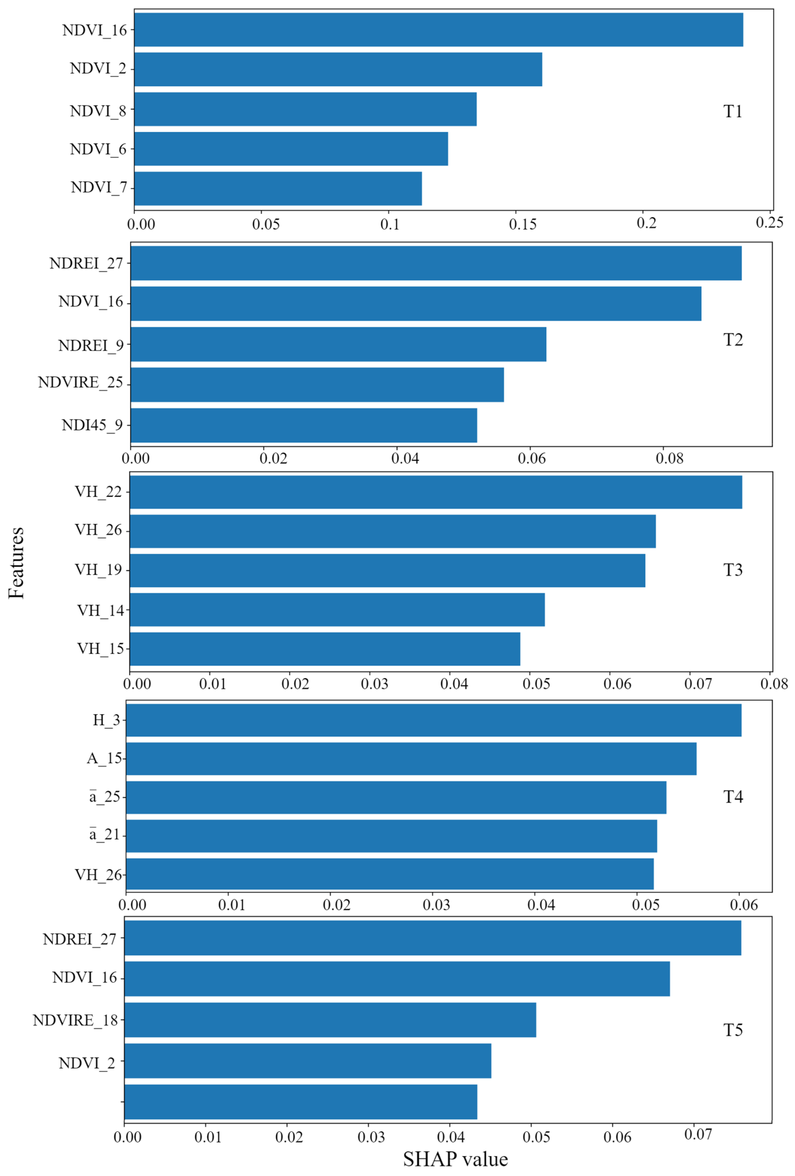
To interpret the performance differences among feature schemes, we analyzed the Random Forest feature-importance rankings and report the top five variables for each scheme (Figure 15). The importance patterns provide an interpretable indication of which temporal observations and feature types most strongly drive classification decisions.

For the NDVI-only feature set (T1), the highest-ranked features are primarily associated with specific temporal dimensions of NDVI. This pattern indicates that classification performance is driven mainly by vegetation dynamics during particular phenological periods rather than by evenly distributed information across all NDVI time steps, underscoring the limited representational capacity of a single vegetation index in complex forest environments.

After incorporating red-edge indices (T2), the importance ranking becomes more diversified. In addition to NDVI_16, red-edge variables appear among the most influential predictors (e.g., NDre1_27, NDre1_9, NDVIre_25, and NDI45_9). This shift indicates that red-edge sensitive indices contribute complementary information beyond NDVI, helping the model capture subtle biochemical/phenological differences among spectrally similar classes and thereby improving classification performance. This is particularly relevant for broadleaf-related classes (e.g., Other hardwoods and Eucalyptus grandis), for which red-edge indices are more sensitive to chlorophyll and canopy biochemical variability and thus help reduce confusion observed under the NDVI-only setting.

In the backscattering-based feature set (T3), the top-ranked predictors are dominated by VH-polarized backscatter at several acquisition times (e.g., VH_22, VH_26, VH_19, VH_14, and VH_15). This pattern implies that cross-polarized backscatter, which is sensitive to canopy volume scattering and structural variability, provides the primary discriminatory signal in the SAR-only setting. However, the heavy reliance on a single polarization type also reflects limited feature diversity, consistent with the relatively low overall performance of T3.

When polarimetric decomposition parameters are added (T4), the top five features span different SAR-derived descriptors, including decomposition parameters (e.g., H_3 and A_15) together with $\overline{\alpha }$ variables and VH backscatter. This mixed composition suggests that combining backscatter intensity with decomposition descriptors enables the classifier to exploit complementary scattering information, improving SAR-only classification compared with T3, although confusion among structurally similar upland classes remains (Table 9). From a class perspective, SAR-derived structural and polarimetric descriptors are likely most informative for canopy structure and moisture regime driven targets such as mangrove and Pinus elliottii, whose scattering responses are strongly modulated by canopy geometry and (for mangroves) intertidal hydrological conditions.

In the full multi-source fusion scheme (T5), the most influential predictors arise from multiple feature groups, with red-edge variables (e.g., NDre1_27 and NDVIre_18) appearing alongside NDVI variables (e.g., NDVI_16 and NDVI_2). This balanced importance structure indicates that the classifier integrates phenology-sensitive optical information with complementary features rather than depending on a single variable type, which aligns with the superior OA/Kappa and consistently high class-wise PA/UA achieved by T5 (Table 9, Figure 12 and Figure 13).

Overall, the top five feature importance analysis demonstrates that improvements in classification performance are closely associated with the diversity and complementarity of feature combinations rather than with the dominance of individual features. This finding provides an interpretable explanation for the performance advantages observed in multi-feature fusion strategies.

4. Discussion

Remote sensing has been widely used for forest species identification. Traditional methods primarily rely on single vegetation indices (e.g., NDVI) or SAR backscattering features as the main classification basis. However, these approaches have not fully exploited the potential of Sentinel-2 red-edge bands and Sentinel-1 polarimetric decomposition parameters for identifying complex forest stands in subtropical regions. This study addresses the need for accurate mapping of typical tree species in subtropical areas by systematically evaluating the effects of optical and SAR multi-source features on classification performance through five feature combinations (T1–T5). The aim is to overcome the limitations of traditional single-source classification methods and establish a multi-source fused remote sensing feature system to enhance the identification capability and spatial representation quality of complex forest stands.

In terms of classification accuracy, the integration of red-edge indices (T2) and polarimetric decomposition features (T4) significantly improved recognition performance compared to single feature sets (T1, T3). The full feature fusion set (T5) achieved the highest accuracy (OA = 95.33%, Kappa = 0.94), demonstrating the potential of multi-feature fusion for tree species recognition in subtropical regions. These results are consistent with ecological and ecophysiological, indicating that canopy reflectance and radar scattering responses are jointly shaped by foliage traits and structural attributes. For example, Noda et al. (2021) showed that seasonal and structural changes in canopy leaf properties directly affect spectral profiles through the growing season, highlighting the importance of phenological and structural factors in optical responses associated with different species traits [50]. Similarly, variations in light transmittance driven by canopy composition and architecture influence spectral and structural signatures across forest types, underscoring the ecological basis for improved classification when combining spectral and polarimetric indicators [51].

The red-edge band significantly enhanced the classification ability for Acacia and Mangrove forests due to its sensitivity to chlorophyll changes. Polarimetric decomposition parameters performed particularly well in identifying Mangrove forests, especially in wetland regions where scattering entropy (H) [52,53] is low, and anisotropy (A) is high [54]. From an ecological perspective, mangrove trees develop specialized structural adaptations (e.g., pneumatophores and prop roots) to cope with hypoxic and saline soils, which affect canopy structure and thus radar backscatter characteristics in predictable ways [55]. This demonstrates a typical polarimetric response pattern, reflecting differences in tree species structure and scattering mechanisms, and confirms the importance of forest stand morphological features in remote sensing classification. In structurally similar species such as Pinus elliottii and Pinus massoniana, subtle morphological differences may lead to unique scattering responses, indicating that microstructural traits also merit further ecological study. Importantly, the feature-importance rankings (Figure 15) corroborate these mechanisms by showing that red-edge variables and SAR-derived structural descriptors enter the top contributors when available, consistent with the observed accuracy gains under multi-feature schemes.

From a feature correlation perspective, the correlation between NDVI and NDVIre/NDre1 was generally high (>0.8), while NDI45 exhibited low correlation with red-edge indices, indicating strong independence. Among polarimetric parameters, scattering entropy (H) was strongly positively correlated with mean scattering angle ($\overline{\alpha }$) (r > 0.88), and both were negatively correlated with anisotropy (A) (r < −0.9), indicating significant redundancy between the latter two, necessitating streamlined selection. These patterns align with ecological theory, suggesting that canopy optical traits and structural traits interact non-linearly across species and functional types, thus requiring integrated feature selection to capture multidimensional differences. Consistent with this, Figure 15 shows that high-performing schemes rely on a diversified set of influential predictors rather than multiple highly collinear variables, providing an interpretable link between redundancy control and classification robustness.

In terms of the spatial configuration of classification results, multi-feature combinations showed significant advantages in highly heterogeneous areas [56], particularly in Mangrove forests, broadleaf forests, and mixed zones of Pinus massoniana and Acacia. Feature fusion effectively alleviated patch fragmentation and misclassification, improving boundary integrity and internal consistency, demonstrating the stronger adaptability of multi-source features to forest stand complexity [57].

In conclusion, red-edge indices and SAR polarimetric parameters provide new information dimensions for improving tree species classification accuracy. They not only compensate for the shortcomings of traditional indices at spectral and structural levels but also exhibit strong differentiation potential in cloudy and rainy southern regions with highly overlapping vegetation. This provides theoretical support for constructing more robust and universally applicable remote sensing classification models for subtropical woodlands.

However, several limitations remain. First, the currently used features primarily focus on spectral and polarimetric scattering dimensions, without considering the potential effects of non-spectral factors such as canopy height, topographic features, and anthropogenic disturbances on tree species identification [58]. Second, although SAR polarimetric parameters excel in Mangrove identification, confusion remains for structurally similar conifers, necessitating further exploration of microstructural differences. Although polarimetric decomposition features significantly improved overall recognition accuracy, confusion persisted in mixed conifer regions, indicating that distinguishing structurally similar stands remains a major challenge for classification models. Additionally, this study used the Random Forest classification method. Future work may explore more expressive deep-learning models, such as multimodal Transformers or graph neural networks, to better exploit cross-sensor relationships, improve performance in highly heterogeneous woodlands, and enhance cross-region generalization.

5. Conclusions

This study developed and evaluated a multi-source, multi-temporal feature-fusion framework for subtropical tree-species mapping by integrating Sentinel-2 optical indices (including red-edge time-series information) with Sentinel-1 SAR backscatter and polarimetric decomposition descriptors. Rather than introducing a new classifier, the main contribution lies in the structured construction, redundancy-controlled selection, and interpretable evaluation of complementary optical–SAR features for fine-scale species discrimination under persistent cloud cover.

The main findings are as follows:

(1) Red-edge time-series indices provide complementary discriminatory information beyond NDVI, improving separability for spectrally similar and broadleaf-related classes. In particular, NDI45 contributes relatively independent information due to its lower correlation with other red-edge indices, strengthening the optical feature space.

(2) SAR scattering descriptors are especially informative for mangrove mapping, where distinctive eco-hydrological settings and canopy–substrate interactions are associated with characteristic polarimetric responses (e.g., relatively low H and higher A), enabling robust separation from upland forest types.

(3) Redundancy control is essential for stable modelling. Correlation analysis indicates substantial collinearity among several vegetation indices and among decomposition parameters. Applying correlation-guided screening (|r| > 0.80) and prioritizing temporally discriminative variables helps reduce redundant encoding while preserving complementary information.

(4) Multi-source fusion governs performance gains. The full fusion scheme (T5) achieves the best overall performance (OA = 95.33%, Kappa = 0.94), outperforming single-source baselines and yielding consistently high class-wise reliability, confirming the synergistic value of combining red-edge optical information with SAR backscatter and polarimetric features.

Overall, integrating multi-temporal red-edge optical features with SAR scattering descriptors provides a robust and high-accuracy pathway for tree-species identification in complex subtropical forests under cloudy and rainy conditions. Future work should incorporate additional structural and environmental factors (e.g., canopy height, topography, and habitat context) and explore more advanced multimodal learning and transfer strategies to further improve generalizability and ecological interpretability.

References

1. Nirhamo, A.; Aakala, T.; Kouki, J. Forest biodiversity in boreal Europe: Species richness and turnover among old-growth forests, managed forests and clearcut sites. Biol. Conserv. 2025, 306, 111147. [Google Scholar] [CrossRef]
2. Costanza, R.; d’Arge, R.; Groot, R.; Farber, S.; Grasso, M.; Hannon, B.; Limburg, K.; Naeem, S.; O’Neill, R.; Paruelo, J.; et al. The value of the world’s ecosystem services and natural capital. Ecol. Econ. 1998, 25, 3–15. [Google Scholar] [CrossRef]
3. United Nations. Transforming Our World: The 2030 Agenda for Sustainable Development. Available online: https://sdgs.un.org/publications/transforming-our-world-2030-agenda-sustainable-development-17981 (accessed on 2 November 2025).
4. Saarela, S.; Andersen, H.E.; Grafström, A.; Schnell, S.; Gobakken, T.; Næsset, E.; Nelson, R.F.; McRoberts, R.E.; Gregoire, T.G.; Ståhl, G. A new prediction-based variance estimator for two-stage model-assisted surveys of forest resources. Remote Sens. Environ. 2017, 192, 1–11. [Google Scholar] [CrossRef]
5. Baldo, M.; Buldrini, F.; Chiarucci, A.; Rocchini, D.; Zannini, P.; Ayushi, K.; Ayyappan, N. Remote sensing analysis on primary productivity and forest cover dynamics: A Western Ghats India case study. Ecol. Inform. 2023, 73, 101922. [Google Scholar] [CrossRef]
6. Markus, I.; Clement, A.; Tatjana, K. Suitability of WorldView-2 data for tree species classification with special emphasis on the four new spectral bands. Photogramm. Fernerkund. Geoinf. 2012, 2012, 573–588. [Google Scholar] [CrossRef]
7. Ferraz, D.P.G.B.; Vicens, R.S. Comparison between machine learning classification and trajectory-based change detection for identifying eucalyptus areas in Landsat time series. Remote Sens. Appl. 2025, 37, 101444. [Google Scholar] [CrossRef]
8. Freudenberg, M.; Schnell, S.; Magdon, P. A Sentinel-2 machine learning dataset for tree species classification in Germany. Earth Syst. Sci. Data 2025, 17, 351–367. [Google Scholar] [CrossRef]
9. European Space Agency. Biomass—ESA’s Forest Mission. Available online: https://www.esa.int/Applications/Observing_the_Earth/FutureEO/Biomass (accessed on 12 November 2025).
10. Zhao, Y.; Zhang, T. Mapping forest tree species using Sentinel-2 time series by taking into account tree age. Forests 2024, 15, 474. [Google Scholar] [CrossRef]
11. Zhang, S.; Yang, S.; Huang, J.; Yang, D.; Zhang, S.; Zhang, J.; Bai, Y. Global-scale improvement of the estimation of terrestrial gross primary productivity by integrating optical and microwave remote sensing with meteorological data. Ecol. Inform. 2024, 83, 102780. [Google Scholar] [CrossRef]
12. Prudente, V.H.R.; Martins, V.S.; Vieira, D.C.; Silva, N.R.F.; Adami, M.; Sanches, I.D.A. Limitations of cloud cover for optical remote sensing of agricultural areas across South America. Remote Sens Appl. 2020, 20, 100414. [Google Scholar] [CrossRef]
13. Kumar, T.; Patnaik, C. Discrimination of Mangrove forests and characterization of adjoining land cover classes using temporal C-band Synthetic Aperture Radar data: A case study of Sundarbans. Int. J. Appl. Earth Obs. 2013, 23, 119–131. [Google Scholar] [CrossRef]
14. Qin, T.; Zhao, Q. Multi-branch and multi-label tree species classification using multimodal remote sensing data. Sci. Rep. 2025, 15, 32710. [Google Scholar] [CrossRef] [PubMed]
15. Aranguren, I.; González-Audícana, M.; Montero, E.; Sanz, J.A.; Álvarez-Mozos, J. Assessing the synergistic use of Sentinel-1, Sentinel-2, and LiDAR data for forest type and species classification. Remote Sens. 2025, 17, 2028. [Google Scholar] [CrossRef]
16. Tan, J.; Li, X.; Chen, Y.; Yan, X.; Huo, Z. Leveraging Sentinel-1/2 time series and deep learning for forest tree species and biodiversity mapping. Front. For. Glob. Change 2025, 8, 1599510. [Google Scholar] [CrossRef]
17. Li, Y.; Liu, T.; Wang, Y.; Duan, L.; Li, M.; Zhang, J.; Zhang, G. A more effective approach for species-level classifications using multi-source remote sensing data: Validation and application to an arid and semi-arid grassland. Ecol. Indic. 2024, 160, 111853. [Google Scholar] [CrossRef]
18. Dong, J.; Xiao, X.; Chen, B.; Torbick, N.; Jin, C.; Zhang, G.; Biradar, C. Mapping deciduous rubber plantations through integration of PALSAR and multi-temporal Landsat imagery. Remote Sens. Environ. 2013, 134, 392–402. [Google Scholar] [CrossRef]
19. Gutiérrez-Vélez, V.H.; DeFries, R. Annual multi-resolution detection of land cover conversion to oil palm in the Peruvian Amazon. Remote Sens. Environ. 2013, 129, 154–167. [Google Scholar] [CrossRef]
20. Food and Agriculture Organization of the United Nations (FAO). SEPAL: A Powerful, Open-Source Platform for Forest and Land Monitoring. Available online: https://www.fao.org/in-action/sepal/overview/sepal-a-powerful-open-source-platform-for-forest-and-land-monitoring/en (accessed on 25 October 2025).
21. Cóndor-Golec, R.D.; Kukharava, M.; Poultouchidou, A. Pathways to Forest Data Transparency: Best Practices from National Forest Monitoring to Support Climate Action; FAO: Rome, Italy, 2024. [Google Scholar] [CrossRef]
22. Orynbaikyzy, A.; Gessner, U.; Mack, B.; Conrad, C. Crop Type Classification Using Fusion of Sentinel-1 and Sentinel-2 Data: Assessing the Impact of Feature Selection, Optical Data Availability, and Parcel Sizes on the Accuracies. Remote Sens. 2020, 12, 2779. [Google Scholar] [CrossRef]
23. Zhao, Z.; Islam, F.; Waseem, L.A.; Tariq, A.; Nawaz, M.; Islam, I.U.; Bibi, T.; Rehman, N.U.; Ahmad, W.; Aslam, R.W.; et al. Comparison of Three Machine Learning Algorithms Using Google Earth Engine for Land Use Land Cover Classification. Rangel. Ecol. Manag. 2024, 92, 129–137. [Google Scholar] [CrossRef]
24. Balabathina, V.N.; Mishra, S.; Sharma, M.; Sharma, S.; Kumar, P.; Narayan, A. Comparative evaluation of fast-learning classification algorithms for urban forest tree species identification using EO-1 hyperion hyperspectral imagery. Front. Environ. Sci. 2025, 13, 1668746. [Google Scholar] [CrossRef]
25. Huang, J.; Piao, R.; Liang, L. Estimation of Canopy Coverage Based on Multisource Remote Sensing Data. IEEE J. Sel. Top. Appl. Earth Obs. Remote Sens. 2025, 18, 21342–21354. [Google Scholar] [CrossRef]
26. Dong, J.; Guo, R.; Lin, M.; Guo, F.; Zheng, X. Multi-objective optimization of green roof spatial layout in high-density urban areas-A case study of Xiamen Island, China. Sustain. Cities Soc. 2024, 115, 105827. [Google Scholar] [CrossRef]
27. Ren, Y.; Wei, X.; Wang, D.; Luo, Y.; Song, X.; Wang, Y.; Yang, Y.; Hua, L. Linking landscape patterns with ecological functions: A case study examining the interaction between landscape heterogeneity and carbon stock of urban forests in Xiamen, China. For. Ecol. Manag. 2013, 293, 122–131. [Google Scholar] [CrossRef]
28. Dai, S.; Zhao, W.; Wang, Y.; Huang, X.; Chen, Z.; Lei, J.; Stein, A.; Jia, P. Assessing spatiotemporal bikeability using multi-source geospatial big data: A case study of Xiamen, China. Int. J. Appl. Earth Obs. 2023, 125, 103539. [Google Scholar] [CrossRef]
29. Bjerreskov, K.S.; Nord-Larsen, T.; Fensholt, R. Classification of Nemoral Forests with Fusion of Multi-Temporal Sentinel-1 and 2 Data. Remote Sens. 2021, 13, 950. [Google Scholar] [CrossRef]
30. Drusch, M.; Bello, U.D.; Carlier, S.; Colin, O.; Fernandez, V.; Gascon, F.; Hoersch, B.; Isola, C.; Laberinti, P.; Martimort, P.; et al. Sentinel-2: ESA’s Optical High-Resolution Mission for GMES Operational Services. Remote Sens. Environ. 2012, 120, 25–36. [Google Scholar] [CrossRef]
31. Xue, J.; Su, B. Significant remote sensing vegetation indices: A review of developments and applications. J. Sens. 2017, 2017, 1353691. [Google Scholar] [CrossRef]
32. Zhang, L.; Chang, A.; Xiang, X. Random forest for intermediate descriptor fusion in shot boundary detection. J. Electron. (China) 2014, 31, 465–472. [Google Scholar] [CrossRef]
33. Kanke, Y.; Tubaña, B.; Dalen, M.; Harrell, D. Evaluation of red and red-edge reflectance-based vegetation indices for rice biomass and grain yield prediction models in paddy fields. Precis. Agric. 2016, 17, 507–530. [Google Scholar] [CrossRef]
34. Becker, F.; Choudhury, B.J. Relative sensitivity of normalized difference vegetation Index (NDVI) and microwave polarization difference Index (MPDI) for vegetation and desertification monitoring. Remote Sens. Environ. 1988, 24, 297–311. [Google Scholar] [CrossRef]
35. Amaro, R.P.; Todoroff, P.; Christina, M.; Duft, D.G.; Luciano, A.C.d.S. Performance evaluation of Sentinel-2 imagery, agronomic and climatic data for sugarcane yield estimation. Comput. Electron. Agric. 2025, 237, 110522. [Google Scholar] [CrossRef]
36. David, R.M.; Rosser, N.J.; Donoghue, D.N.M. Improving above ground biomass estimates of Southern Africa dryland forests by combining Sentinel-1 SAR and Sentinel-2 multispectral imagery. Remote Sens. Environ. 2022, 282, 113232. [Google Scholar] [CrossRef]
37. Shirkey, G.; John, R.; Chen, J.; Dahlin, K.; Abraha, M.; Sciusco, P.; Lei, C.; Reed, D.E. Fine resolution remote sensing spectra improves estimates of gross primary production of croplands. Agric. For. Meteorol. 2022, 326, 109175. [Google Scholar] [CrossRef]
38. Lee, J.S.; Grunes, M.R.; Pottier, E.; Ferro-Famil, L. Unsupervised terrain classification preserving polarimetric scattering characteristics. IEEE Trans. Geosci. Remote Sens. 2004, 42, 722–731. [Google Scholar] [CrossRef]
39. Cloude, S.R.; Pottier, E. An entropy based classification scheme for land applications of polarimetric SAR. IEEE Trans. Geosci. Remote Sens. 1997, 35, 68–78. [Google Scholar] [CrossRef]
40. Hong, T.; Yim, S.H.L.; Heo, Y. Interpreting complex relationships between urban and meteorological factors and street-level urban heat islands: Application of random forest and SHAP method. Sustain. Cities Soc. 2025, 126, 106353. [Google Scholar] [CrossRef]
41. Kim, Y.; Kim, Y. Explainable heat-related mortality with random forest and SHapley Additive exPlanations models. Sustain. Cities Soc. 2022, 79, 103677. [Google Scholar] [CrossRef]
42. Huang, X.; Wang, H.; Li, X. A multi-scale semantic feature fusion method for remote sensing crop classification. Comput. Electron. Agric. 2024, 224, 109185. [Google Scholar] [CrossRef]
43. Davis, C.C.; Lyra, G.M.; Park, D.S.; Asprino, R.; Maruyama, R.; Torquato, D.; Cook, B.I.; Ellison, A.M. New directions in tropical phenology. Trends Ecol. Evol. 2022, 37, 683–693. [Google Scholar] [CrossRef]
44. Vergara, J.R.; Estévez, P.A. A review of feature selection methods based on mutual information. Neural Comput. Appl. 2015, 24, 175–186. [Google Scholar] [CrossRef]
45. Hanberry, B.B. Practical guide for retaining correlated climate variables and unthinned samples in species distribution modeling, using random forests. Ecol. Inform. 2023, 78, 102406. [Google Scholar] [CrossRef]
46. Koh, J.C.O.; Banerjee, B.P.; Spangenberg, G.; Kant, S. Automated hyperspectral vegetation index derivation using a hyperparameter optimisation framework for high-throughput plant phenotyping. New Phytol. 2022, 233, 2659–2670. [Google Scholar] [CrossRef]
47. Ming, W.; Zhang, Q.; Liu, X.; Zhang, J.; Yu, F.; Zhang, X.; Zhao, R. Research progress on multimodal data fusion in forest resource monitoring. Front. Plant Sci. 2025, 16, 1710618. [Google Scholar] [CrossRef]
48. Fundisi, E.; Tesfamichael, S.G.; Ahmed, F. A combination of Sentinel-1 RADAR and Sentinel-2 multispectral data improves classification of morphologically similar savanna woody plants. Eur. J. Remote Sens. 2022, 55, 372–387. [Google Scholar] [CrossRef]
49. Wu, Y.; Lu, C.; Wu, K.; Gao, W.; Yang, N.; Lin, J. Advancements and trends in mangrove species mapping based on remote sensing: A comprehensive review and knowledge visualization. Glob. Ecol. Conserv. 2025, 57, e03408. [Google Scholar] [CrossRef]
50. Noda, H.; Muraoka, H.; Nasahara, K.N. Plant ecophysiological processes in spectral profiles: Perspective from a deciduous broadleaf forest. J. Plant Res. 2021, 134, 737–751. [Google Scholar] [CrossRef]
51. Williams, L.J. Tree diversity shapes the spectral signature of light transmitted through canopies. Ecology 2025, 106, e70032. [Google Scholar] [CrossRef] [PubMed]
52. Chen, J.; Liang, X.; Liu, Z.; Gong, W.; Chen, Y.; Hyyppä, J.; Kukko, A.; Wang, Y. Tree species recognition from close-range sensing: A review. Remote Sens. Environ. 2024, 313, 114337. [Google Scholar] [CrossRef]
53. Liang, X.; Chen, J.; Gong, W.; Puttonen, E.; Wang, Y. Influence of data and methods on high-resolution imagery-based tree species recognition considering phenology: The case of temperate forests. Remote Sens. Environ. 2025, 323, 114654. [Google Scholar] [CrossRef]
54. Mu, Y.; Guo, J.; Shahzad, M.; Zhu, X. National-scale tree species mapping with deep learning reveals forest management insights in Germany. Int. J. Appl. Earth Obs. 2025, 139, 104522. [Google Scholar] [CrossRef]
55. Liu, W. Seasonal and vertical variation in canopy structure and leaf spectral properties determine the canopy reflectance of a rice field. Agric. For. Meteorol. 2024, 355, 110132. [Google Scholar] [CrossRef]
56. Polyakova, A.; Mukharamova, S.; Yermolaev, O.; Shaykhutdinova, G. Automated Recognition of Tree Species Composition of Forest Communities Using Sentinel-2 Satellite Data. Remote Sens. 2023, 15, 329. [Google Scholar] [CrossRef]
57. Ma, Y.; Lou, H.; Yan, M.; Sun, F.; Li, G. Spatio-temporal fusion graph convolutional network for traffic flow forecasting. Inf. Fusion 2024, 104, 102196. [Google Scholar] [CrossRef]
58. Wu, Y.; Hong, C.; Zhang, X.; He, Y. Stack-based Scale-recurrent Network for Face Image Deblurring. Neural Process. Lett. 2021, 53, 4419–4436. [Google Scholar] [CrossRef]
Figure 1. Location of the study area.
Remotesensing 18 00592 g001
Figure 2. Photographs of typical tree species in the study area: (a) Pinus massoniana, (b) Pinus elliottii, (c) Acacia, (d) Eucalyptus grandis, and (e) Mangrove forest. All photographs and UAV images shown in this figure were acquired by the authors during field surveys conducted between December 2021 and December 2022.
Remotesensing 18 00592 g002
Figure 3. Workflow of the proposed framework.
Remotesensing 18 00592 g003
Figure 4. Spectral curves of typical tree species in different months ((a) Pinus massoniana, (b) Pinus elliottii, (c) Acacia, (d) Eucalyptus grandis, (e) Other hardwoods, and (f) Mangrove forest).
Remotesensing 18 00592 g004
Figure 5. Spectral time series curves of typical tree species ((a) Pinus massoniana, (b) Pinus elliottii, (c) Acacia, (d) Eucalyptus grandis, (e) Other hardwoods, and (f) Mangrove forest).
Remotesensing 18 00592 g005
Figure 6. Time curves of backscattering coefficients of each tree species after filtering. ((a) VH polarization; (b) VV polarization).
Remotesensing 18 00592 g006
Figure 7. Backscattering coefficients (dB) of tree species in January–December. ((al): January–December).
Remotesensing 18 00592 g007
Figure 8. Temporal profiles of polarimetric decomposition parameters for the six tree classes after speckle filtering: (a) scattering entropy (H), (b) anisotropy (A), and (c) mean scattering angle ( α ¯ ). The x-axis (1–28) denotes the acquisition order of Sentinel-1 observations (Table 1), and the y-axis shows the class-level mean parameter values.
Remotesensing 18 00592 g008
Figure 9. Monthly distributions of polarimetric decomposition parameters (H, A, and α ¯ ) for the six tree classes. Panels (al) correspond to January–December. Boxplots summarize within-class variability; the left y-axis applies to H and A, and the right y-axis applies to α ¯ .
Remotesensing 18 00592 g009
Figure 10. Correlation matrices of four vegetation indices (NDVI, NDI45, NDre1, and NDVIre) derived from the Sentinel-2 time series. Each panel corresponds to one Sentinel-2 acquisition (indexed as 1–29; see Table 2), and values denote Pearson correlation coefficients (r) among the four indices at the same acquisition. Color indicates correlation strength (−1 to 1), highlighting periods of strong redundancy (e.g., |r| > 0.80) versus complementary behavior (e.g., |r| < 0.70) used for feature screening.
Remotesensing 18 00592 g010
Figure 11. Correlation matrices of Sentinel-1 SAR scattering features for the six tree classes across the 28 acquisitions (indexed as 1–28; see Table 1). Each panel shows Pearson correlation coefficients among VV and VH backscatter and the polarimetric decomposition parameters (H, A, and α ¯ ) at the same acquisition. Color indicates correlation strength (−1 to 1), supporting redundancy screening of SAR feature variables.
Remotesensing 18 00592 g011
Figure 12. Overall accuracy (OA) and Kappa coefficient of Random Forest classification under the five feature-combination schemes (T1–T5). Bars compare the OA and Kappa values obtained for each feature scheme.
Remotesensing 18 00592 g012
Figure 13. Comparison of PA and UA accuracy based on random forests: (a) Producer’s Accuracy (PA) for different tree species under feature sets T1–T5, and (b) User’s Accuracy (UA) for different tree species under feature sets T1–T5.
Remotesensing 18 00592 g013
Figure 14. Comparison of local classification effects of tree species with different feature combinations using random forest classification.
Remotesensing 18 00592 g014
Figure 15. Top five feature-importance rankings for each feature scheme (T1–T5) derived from the Random Forest model. Subscripts denote acquisition indices of Sentinel-2 (for vegetation indices) and Sentinel-1 (for SAR features), consistent with Table 1 and Table 2.
Remotesensing 18 00592 g015