Thick Cloud Removal in Multitemporal Remote Sensing Images via Sobel-Consistency and Subspace-Based Spatiospectral Low-Rank Tensor Regularization

Highlights

What are the main findings?

• A Sobel-consistency regularization is introduced to exploit the edge consistency in multitemporal remote sensing images.
• A unified thick cloud removal model combines Sobel-based edge consistency with subspace-driven spatiospectral low-rank tensor regularization, solved via an efficient proximal alternating minimization algorithm.

What are the implications of the main findings?

• Compared with most existing methods, the proposed approach achieves higher reconstruction accuracy and better visual quality under heavy cloud coverage.
• The method offers a robust and general solution for thick cloud removal in multitemporal remote sensing images.

Abstract

Thick cloud removal is a critical preprocessing step for multitemporal remote sensing images (MTRSIs), as it directly determines the reliability of downstream analysis and applications. In MTRSIs, the same geographic region is observed at different times, and the underlying edge structures often remain physically consistent across temporal observations. Leveraging this intrinsic property, we introduce a Sobel-consistent term that explicitly enforces temporal consistency of edge-related features, thereby improving the reconstruction of fine structures and textures in cloud-obscured regions. Building on this insight, we propose a novel thick cloud removal model that integrates Sobel-based edge consistency with subspace-based spatiospectral low-rank tensor regularization. In this model, intrinsic images derived from subspace representation are organized into a fourth-order tensor, and low-rank constraints are applied to jointly capture the spatial, spectral, and temporal correlations inherent in MTRSIs. To efficiently solve the resulting optimization problem, we introduce an algorithm based on proximal alternating minimization. Experiments on both simulated and real-world MTRSI datasets demonstrate that the proposed method achieves superior reconstruction accuracy and visual fidelity, validating the physical interpretability and effectiveness of the approach.

1. Introduction

With recent advances in remote sensing and imaging hardware, optical remote sensing data with higher spatial and spectral resolutions have become increasingly accessible. Owing to the periodic orbits of satellites, remote sensing observations can be repeatedly acquired over the same region, forming MTRSIs. These data integrate spatial, spectral, and temporal information, enabling precise land-cover description, accurate classification, and continuous monitoring of surface dynamics [1,2]. However, frequent cloud cover leads to severe information loss in certain temporal frames. Clouds obscure large spatial areas and simultaneously degrade all spectral bands, thereby affecting downstream tasks such as super-resolution and spectral unmixing. As a result, restoring cloud- and shadow-contaminated regions in MTRSIs remains a critical yet challenging problem [3,4].

1.1. Related Works

Existing cloud removal methods for MTRSIs typically exploit spatial, spectral, and/or temporal priors to restore cloud-contaminated regions, and can be broadly categorized into spatial-based, spectral-based, and temporal-based approaches.

Spatial-based methods rely on inpainting techniques driven exclusively by spatial-domain characteristics. They assume that cloudy and cloud-free regions exhibit similar textural patterns, enabling the recovery of missing information from local or nonlocal pixels in unobscured areas [5,6]. Zhu et al. proposed a modified neighborhood similar pixel interpolator for thick cloud removal, which incorporates contextual multiple linear prediction to effectively mitigate edge artifacts [7]. Other methods that model spatial variations or adopt exemplar-based inpainting have also shown strong performance [8]. For instance, the RCTV model [9] applies total variation regularization on decomposition coefficients, enhancing cloud removal while preserving texture details with high computational efficiency. However, when cloud coverage is extensive, the amount of usable spatial information is limited, restricting the applicability of purely spatial-based strategies. Thus, these methods are most effective when cloud-affected regions are relatively small and contain simple structures [10]. Spectral-based methods exploit priors along the spectral dimension. Lv et al. [11] incorporated supplementary spectral information to compensate for distortions caused by sensor failures or thin clouds, whereas Xu et al. [12] jointly utilized spatial and multi-spectral cues to more accurately estimate the cloud signal-to-noise ratio. Yet, in practical MTRSIs, dense clouds simultaneously corrupt all spectral bands, resulting in insufficient reliable spectral references. Consequently, relying solely on spatial or spectral information is insufficient for robust cloud removal [13]. Xu et al. proposed the Haar nuclear norm (HNN) for remote sensing image restoration, which transforms images into wavelet coefficients to separate low-frequency coarse structures and high-frequency fine details, and enforces low-rankness via nuclear norms for efficient reconstruction [14]. Temporal-based methods leverage the intrinsic correlations among multitemporal observations, considering that satellites repeatedly capture the same area, but cloud coverage varies across time. Wang et al. introduced a fast spatial-–spectral random forest (FSSRF) method based on the SSRF framework, significantly improving computational efficiency while maintaining high reconstruction accuracy [15]. Nevertheless, these methods still face challenges in accurately refining uncontaminated reference features to ensure consistency with the target images.

Hybrid cloud removal methods integrate spatial, spectral, and temporal information within unified frameworks to enhance reconstruction accuracy and robustness under complex conditions such as thick cloud coverage or rapid temporal changes. Considering spatial–spectral consistency, Chen et al. employed slow feature analysis (SFA) with a spatio-spectral correction strategy to extract slowly varying features and suppress high-reflectance interference [16]. Li et al. further proposed a fully-connected extended tensor network with total variation regularization for remote sensing image completion [17]. Spatial–temporal coherence has been exploited through weighted regression models [18] and spatiotemporal patch segmentation [19].

To better capture global structural correlations, Zheng et al. introduced a generalized tensor decomposition framework (FCTN) for thick cloud removal [20], while Qiu et al. proposed an unfolding-induced tensor nuclear norm (OTNN) [21]. Xiao et al. developed an ${\mathsf{\ell }}_0$-norm tensor rank minimization model with guaranteed convergence (L0-TC) [22]. Deep learning has also been incorporated: spatial–temporal patch groups [23] and deep spatial–temporal priors combined with t-SVD have shown strong performance for gap-filling and thick cloud removal [24]. Joint spectral–temporal strategies, including contextual nonlinear reconstruction [25] and robust matrix completion [26], have also been explored.

More recently, spatial–spectral–temporal (SST) models have demonstrated strong potential. Internal deep image priors [27], and SST connective tensor network decomposition (SSTC-CR) [28] can recover cloud-covered areas without auxiliary cloud-free data. Additional efforts include tensor ring completion with TV regularization (TRTV) [29] and TVLRSDC, a unified detection–removal framework leveraging spatial–spectral TV constraints [30]. To overcome the limitations of hand-crafted priors and the high cost of labeled datasets, Chen et al. [31] proposed a model-driven method combining low-rank sparse decomposition with a self-supervised deep prior. Similarly, STLR-DP [32] employs an untrained neural network with spectral–temporal low-rank regularization to reconstruct cloud-contaminated regions from a single observation. Li et al. [33] further incorporated gradient-domain fidelity with low-rank tensor ring regularization, although correlations captured among adjacent dimensions remain limited.

1.2. Motivations and Contributions

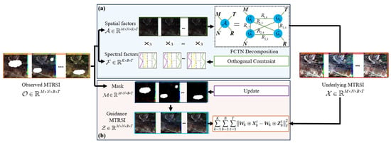
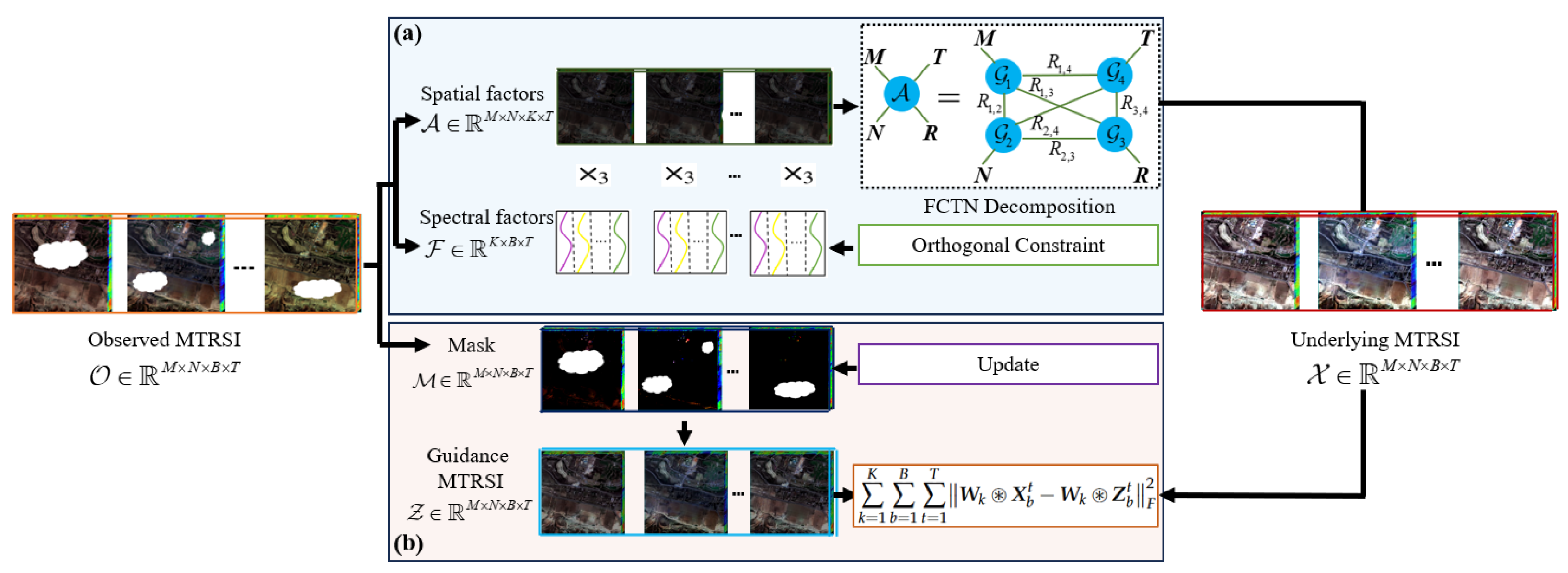
Motivated by the observation that edge structures in MTRSIs remain physically consistent across time, we propose a Sobel-consistency and subspace-based spatiospectral low-rank tensor regularization (SCSSLR) framework. By explicitly enforcing temporal edge consistency, the SCSSLR model leverages both structural priors and low-rank SST correlations to accurately reconstruct cloud-obscured regions while preserving fine details. As shown in Figure 1, an MTRSI is modeled as a fourth-order tensor $\mathcal{X}\in {\mathbb{R}}^{M\times N\times B\times T}$, where a spectral subspace projection is first applied to reduce redundancy and extract compact intrinsic representations. A FCTN decomposition is then performed on the resulting $M\times N\times K\times T$ tensor to effectively capture spatial–spectral–temporal correlations with substantially reduced computational cost. To further preserve structural details, Sobel convolution is employed to extract edge-consistent features, enforcing alignment between the reconstructed latent tensor and the guidance image $\mathcal{Z}$. By jointly modeling low-rank SST dependencies and Sobel-consistency, the proposed SCSSLR framework achieves accurate and structurally coherent thick cloud removal.

Figure 1. Framework of the proposed SCSSLR model for thick cloud removal. (a) The observed MTRSI $\mathcal{O}\in {\mathbb{R}}^{M\times N\times B\times T}$ is projected into a spectral subspace, producing a spatial factor $\mathcal{A}$ and a spectral factor $\mathcal{F}$. FCTN decomposition is applied to $\mathcal{A}$ to capture intrinsic spatial structure, while a semi-orthogonal constraint is imposed on $\mathcal{F}$. (b) Sobel-consistency is enforced between the latent clean image $\mathcal{X}$ and the guidance image $\mathcal{Z}$ to preserve structural details.

The main contributions of this work are summarized as follows:

• We introduce a Sobel-consistency regularization that explicitly enforces edge consistency across multitemporal observations, which preserves fine structural details and suppresses edge blurring in cloud-masked regions. Its effectiveness is validated through comparative experiments with gradient operators as well as dedicated ablation studies, where both visual results and quantitative metrics consistently demonstrate the advantage of the proposed Sobel-consistency regularization.
• We propose a unified Sobel-consistency and subspace-based spatiospectral low-rank framework, which models intrinsic spatiospectral correlations of MTRSIs via a fourth-order tensor constructed in a low-dimensional spectral subspace. Ablation studies that jointly integrate Sobel-consistency priors and low-rank tensor regularization yield consistently superior cloud removal performance compared with using either component alone.
• We introduce an efficient PAM algorithm with an iterative cloud-mask refinement strategy to solve the resulting optimization problem. Extensive experiments on both simulated and real MTRSI datasets demonstrate that the proposed method consistently outperforms state-of-the-art methods in terms of quantitative metrics and visual restoration quality.

This article is organized as follows. Section 2 introduces the notations and preliminaries. Section 2.3 details the SCSSLR model and its PAM-based optimization. Section 3 presents experimental results, Section 4 provides further discussion, and Section 5 concludes the work.

2. Materials and Methods

2.1. Notations

In this section, we present a summary of key notations employed throughout the paper, as outlined in the Table 1 [28].

Table 1. Notations and their interpretations used in this paper.

Notations	Interpretations
x, $\mathit{x}$, $\mathit{X}$, $\mathcal{X}$	Scalar, vector, matrix, tensor.
$\mathcal{X}\in {\mathbb{R}}^{M\times N\times B\times T}$	A MTRSI, where M is spatial height,
	N is spatial width, B is the number of spectral bands,
	and T is the number of time nodes.
$\mathcal{X}(m,n,b,t)$	The $(m,n,b,t)$th element of an fourth-order
	tensor $\mathcal{X}\in {\mathbb{R}}^{M\times N\times B\times T}$.
$\mathit{F}(b,k)$	The $(b,k)$th element of matrix $\mathit{F}\in {\mathbb{R}}^{B\times K}$.
${\parallel \mathcal{X}\parallel }_F$	${\parallel \mathcal{X}\parallel }_F=\sqrt{{\sum }_{m,n,b,t}{\left|\mathcal{X}(m,n,b,t)\right|}^2}$.
${\mathcal{X}}^t$	RSI at the tth time node of $\mathcal{X}\in {\mathbb{R}}^{M\times N\times B\times T}$.
${\mathit{X}}_b^t$	RSI at the tth time node and the bth band
	of $\mathcal{X}\in {\mathbb{R}}^{M\times N\times B\times T}$.
⊙	Component-wise multiplication.
⊘	Component-wise division.
⊗	Kronecker product.

2.2. Preliminary

Furthermore, we provide formal definitions of the mode-3 unfolding and the mode-3 product operations, which are fundamental to the subsequent tensor-based formulations.

Definition 1 

(Mode-3 Unfolding [28]). Let $\mathcal{X}\in {\mathbb{R}}^{M\times N\times B\times T}$ be a fourth-order tensor. Let $(I_1,I_2,I_3,I_4)=(M,N,B,T)$, The mode-3 unfolding of $\mathcal{X}$, denoted as ${\mathit{X}}_{\left(3\right)}$, rearranges the elements of $\mathcal{X}$ into a matrix of size ${\mathbb{R}}^{I_3\times {\prod }_{i\ne 3}{I}_i}$. Specifically, the element $\mathcal{X}(i_1,i_2,i_3,i_4)$ is mapped to the matrix entry ${\mathit{X}}_{\left(3\right)}(i_3,j)$, where the column index is computed by

$$j=1+\sum _{\begin{array}{c}s=1\\ s\ne 3\end{array}}^4(i_s-1)J_s,\mathit{with}{J}_s=\prod _{\begin{array}{c}m=1\\ m\ne 3\end{array}}^{s-1}{I}_m.$$

We use the notation ${\mathit{X}}_{\left(3\right)}={Unfold}_3\left(\mathcal{X}\right)$ to represent the unfolding operation and $\mathcal{X}={Fold}_3\left({\mathit{X}}_{\left(3\right)}\right)$ for its inverse.

Definition 2 

(Mode-3 Product [28]). The mode-3 product of a tensor $\mathcal{A}\in {\mathbb{R}}^{M\times N\times K\times T}$ with a matrix $\mathit{F}\in {\mathbb{R}}^{B\times K}$ results in a tensor $\mathcal{X}\in {\mathbb{R}}^{M\times N\times B\times T}$, denoted as $\mathcal{X}=\mathcal{A}{\times }_3\mathit{F}$, and satisfies:

$$\mathcal{X}(m,n,b,t)=\sum _{k=1}^K\mathcal{A}(m,n,k,t)\mathit{F}(b,k).$$

According to Definitions 1 and 2, the following equivalence holds:

$$\mathcal{O}=\mathcal{X}{\times }_3\mathit{F}\iff {\mathit{O}}_{\left(3\right)}=\mathit{F}{\mathit{X}}_{\left(3\right)}.$$

Based on the above mode-3 product, a cloud-free MTRSI tensor $\mathcal{X}$ can be compactly represented in a low-dimensional spectral subspace. Specifically, the image at the t-th temporal index satisfies:

$${\mathcal{X}}^t={\mathcal{A}}^t{\times }_3{\mathit{F}}_t,$$

where ${\mathcal{A}}^t\in {\mathbb{R}}^{M\times N\times K}$ denotes the intrinsic spatial tensor, ${\mathit{F}}_t\in {\mathbb{R}}^{B\times K}$ is the corresponding spectral basis, and $K\ll B$. Since the spatial structures of the same scene remain largely consistent over time, stacking ${\left\{{\mathcal{A}}^t\right\}}_{t=1}^T$ yields an intrinsic tensor

$$\mathcal{A}=\mathrm{PerT}\left({\mathcal{A}}^{1:T}\right)\in {\mathbb{R}}^{M\times N\times K\times T},$$

which exhibits strong temporal consistency. To characterize the associated spatiospectral low-rank structure while preserving the intrinsic tensor organization, a structured tensor decomposition is required. Moreover, operating in the intrinsic space significantly reduces the computational burden.

Based on this compact representation, the FCTN decomposition is introduced, followed by the formulation of a thick cloud removal model for MTRSIs.

Definition 3 

(FCTN decomposition [20]). Given a tensor $\mathcal{A}\in {\mathbb{R}}^{M\times N\times K\times T}$, its fully-connected tensor network decomposition decomposition is defined by:

$$\begin{array}{cc}\hfill \mathcal{A}(m,n,k,t)=& \sum _{s_{12}=1}^{r_{12}}\sum _{s_{13}=1}^{r_{13}}\sum _{s_{14}=1}^{r_{14}}\sum _{s_{23}=1}^{r_{23}}\sum _{s_{24}=1}^{r_{24}}\sum _{s_{34}=1}^{r_{34}}\hfill \\ \hfill & {\mathcal{G}}_1(m,s_{12},s_{13},s_{14})·{\mathcal{G}}_2(s_{12},n,s_{23},s_{24})·\hfill \\ \hfill & {\mathcal{G}}_3(s_{13},s_{23},k,s_{34})·{\mathcal{G}}_4(s_{14},s_{24},s_{34},t),\hfill \end{array}$$

where ${\mathcal{G}}_1\in {\mathbb{R}}^{M\times r_{12}\times r_{13}\times r_{14}},{\mathcal{G}}_2\in {\mathbb{R}}^{r_{12}\times N\times r_{23}\times r_{24}},{\mathcal{G}}_3\in {\mathbb{R}}^{r_{13}\times r_{23}\times K\times r_{34}},{\mathcal{G}}_4\in {\mathbb{R}}^{r_{14}\times r_{24}\times r_{34}\times T}$ are the core tensors (FCTN factors), and $\mathit{r}=(r_{12},r_{13},r_{14},r_{23},$$r_{24},r_{34}),$ is called the FCTN rank. To simplify notation, the FCTN decomposition is denoted as $\mathcal{A}=FCTN\left({\mathcal{G}}_{1:4}\right),$ and the partial composition excluding the j-th factor is written as ${\mathcal{Q}}_j=FCTN({\mathcal{G}}_{1:4},/{\mathcal{G}}_j),\mathit{for}j=1,2,3,4.$

2.3. Proposed Model for Thick Cloud Removal

In MTRSIs, strong temporal similarity allows cloud-free observations at certain time points to guide the reconstruction of heavily clouded regions. Thus, we first construct a guidance image that exploits the relationship between clear and cloudy areas, and introduce a Sobel-based edge consistency constraint to capture fine structural details. The following section outlines the guidance image construction and Sobel-consistency computation.

2.3.1. Guidance MTRSI

Now, we consider the estimation of the guidance image. Let $\mathcal{O}\in {\mathbb{R}}^{M\times N\times B\times T}$ denote the observed MTRSI, where $\mathbb{F}$ and $\mathbb{C}$ represent the index sets of cloud-free and cloudy regions, respectively. For $(i_1,i_2,i_3,i_4)\in \mathbb{F}$, $\mathcal{O}(i_1,i_2,i_3,i_4)$ corresponds to a clear-sky observation, whereas $(j_1,j_2,j_3,j_4)\in \mathbb{C}$ corresponds to cloud-contaminated conditions. The guidance image $\mathcal{Z}$ is constructed through two steps.

Step 1: Parameter estimation from cloud-free regions. Even in cloudy time frames, some pixels remain unobscured. Let $\Omega$ denote the cloud-free index set and ${\Omega }^c$ its complement, i.e., the cloud-covered set. To model the relationship among cloud-free observations across different time points, we estimate a linear mapping via least squares over the cloud-free region:

$$\underset{a,b}{min}{∥{\mathcal{P}}_{\Omega }\left(\mathcal{O}(j_1,j_2,j_3,j_4)-\sum a\mathcal{O}(i_1,i_2,i_3,i_4)-b\right)∥}_F^2,$$

(1)

where a and b denote the coefficient and bias terms. $\Omega$ is the cloud-free index set (i.e., $\Omega \equiv \mathbb{F}$), and ${\Omega }^c$ is the cloud-covered set (i.e., ${\Omega }^c\equiv \mathbb{C}$). ${\mathcal{P}}_{\Omega }$ (resp. ${\mathcal{P}}_{{\Omega }^c}$) projects entries inside $\Omega$ (resp. ${\Omega }^c$), setting others to zero.

Step 2: Guidance image construction. Using the estimated parameters, the guidance image is defined as

$$\left\{\begin{array}{cc}\mathcal{Z}(i_1,i_2,i_3,i_4)=\mathcal{O}(i_1,i_2,i_3,i_4),\hfill & (i_1,i_2,i_3,i_4)\in \Omega ,\hfill \\ \mathcal{Z}(j_1,j_2,j_3,j_4)=\sum a\mathcal{O}(i_1,i_2,i_3,i_4)+b,\hfill & (j_1,j_2,j_3,j_4)\in {\Omega }^c.\hfill \end{array}\right.$$

(2)

Cloud-free observations are strictly enforced in the guidance image via

$${\mathcal{P}}_{\Omega }\left(\mathcal{Z}\right)={\mathcal{P}}_{\Omega }\left(\mathcal{O}\right).$$

(3)

Remark 1. 

To estimate the guidance image, the relationship between cloud-free and cloud-covered regions is initially modeled using a linear mapping. To statistically evaluate whether this assumption is sufficient, we further compare it with nonlinear alternatives, including a quadratic polynomial model and a nonlinear regression model implemented by nlinfit, where nlinfit is the nonlinear least-squares fitting function in MATLAB. For each formulation, the experiment is independently repeated ten times, and the reconstruction performance is reported as mean ± standard deviation (Std). As shown in Table 2, all three relationship models yield very similar performance on both Africa 2 and America 2 datasets, with overlapping standard deviations across independent runs. No statistically significant performance improvement is observed when adopting nonlinear mappings. These results indicate that the linear model provides a sufficiently reliable and effective representation of the clear–cloudy correspondence while avoiding unnecessary model complexity.

Table 2. Comparison of cloud removal performance (mean ± Std) under different relationship assumptions over ten independent runs.

Relationship Type	Model	Africa 2	America 2
Linear	Linear mapping	$33.07\pm 0.04$	$43.99\pm 0.06$
Nonlinear	Quadratic polynomial	$32.92\pm 0.05$	$43.84\pm 0.06$
	nlinfit	$33.03\pm 0.04$	$43.66\pm 0.07$

Remark 2. 

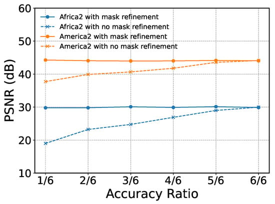
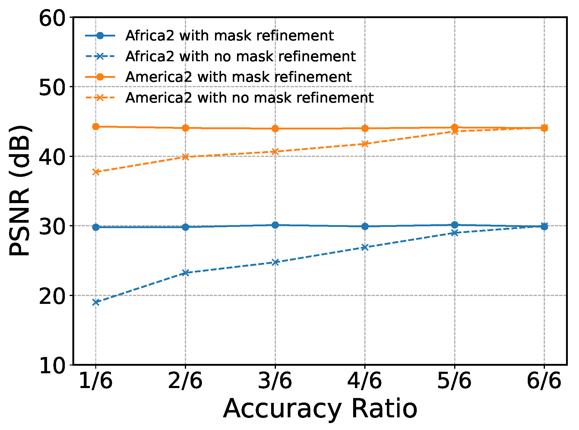
A sensitivity analysis was conducted to examine how reference image quality influences cloud-removal performance. For Africa 2 and America 2 under Case 3, guidance masks were randomly permuted to generate reference images of varying accuracy, and the model was tested with and without mask refinement. As shown in Figure 2, performance degrades noticeably without refinement—high-quality guidance yields better reconstruction—whereas the refinement module stabilizes performance even under severe mask perturbations. This confirms that mask refinement substantially improves robustness to inaccuracies in the guidance images.

Figure 2. Comparison of cloud removal performance at varying accuracy ratios.

2.3.2. Sobel-Consistency

Considering that remote sensing images captured at different time steps along each spectral band often exhibit similar edge structures, a novel Sobel-consistent term is formulated based on the Sobel convolution operator, as detailed below:

$$\sum _{k=1}^K\sum _{b=1}^B\sum _{t=1}^T{∥{\mathit{W}}_k⊛{\mathit{X}}_b^t-{\mathit{W}}_k⊛{\mathit{Z}}_b^t∥}_F^2,$$

where $\mathcal{Z}\in {\mathbb{R}}^{M\times N\times B\times T}$ denotes the guidance image estimated from the observed data, $\mathcal{X}\in {\mathbb{R}}^{M\times N\times B\times T}$ represents the restored image, ${\mathit{W}}_k\in {\mathbb{R}}^{c_1\times c_2}$ for $k=1,2,\dots ,K$ are the Sobel convolutional filters, and ⊛ denotes the convolution operation. The Sobel-consistent term exploits the strong feature extraction capability of convolution operators to preserve fine structures and textures.

In this work, we employ the classical Sobel filters along the horizontal and vertical spatial directions, and thus set $K=2$. The explicit mathematical expressions of the Sobel filters are given by

$${\mathit{W}}_1=\left(\begin{array}{ccc}\hfill -1& \hfill 0& \hfill 1\\ \hfill -2& \hfill 0& \hfill 2\\ \hfill -1& \hfill 0& \hfill 1\end{array}\right),{\mathit{W}}_2=\left(\begin{array}{ccc}\hfill -1& \hfill -2& \hfill -1\\ \hfill 0& \hfill 0& \hfill 0\\ \hfill 1& \hfill 2& \hfill 1\end{array}\right),$$

(4)

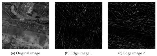
where ${\mathit{W}}_1$ and ${\mathit{W}}_2$ correspond to the Sobel operators for detecting horizontal and vertical edges, respectively. As illustrated in Figure 3, Sobel convolutions applied along the horizontal and vertical spatial directions extract orientation-specific edge features from an example MTRSI slice (the first time point and the first spectral band). By incorporating these Sobel-derived features, the proposed model enforces edge consistency between the reconstructed image and the guidance image, thereby enhancing the recovery of sharp structures and fine spatial details in the final output.

Figure 3. (a) The underlying ${\mathit{X}}_b^t$ image; (b) edge image in the spatial height dimension; (c) edge image in the spatial width dimension.

Remark 3. 

Accurate edge extraction is crucial for cloud detection and structural preservation in remote sensing imagery. Traditional gradient operators, however, are highly susceptible to noise under dense cloud interference. As shown in Table 3, the Sobel operator—combining differentiation with localized smoothing—provides markedly superior edge detection by enhancing structural boundaries while suppressing noise. This makes it particularly effective for scenes with large-scale, thick cloud occlusion.

Table 3. Comparison of Sobel and Gradient methods for thick cloud removal in remote sensing images.

Method	PSNR (dB)	SSIM	SAM	CC
Gradient	24.15	0.782	8.47	0.891
Sobel	24.73	0.805	7.92	0.913

Remark 4. 

Note that the Sobel-consistency term is imposed between the restored image ${\mathit{X}}_b^t$ and the guidance image ${\mathit{Z}}_b^t$. Here, the guidance image ${\mathit{Z}}_b^t$ is not a single-frame reference but is computed by aggregating cloud-free observations from multiple time points, as introduced in the Section 2.3.1. Since cloud coverage varies over time, different pixels are observable at different dates, and ${\mathit{Z}}_b^t$ integrates these cloud-free samples through multitemporal fitting to form a guidance structure. If the guidance image ${\mathit{Z}}_b^t$ is removed, edge consistency can be alternatively enforced directly between adjacent reconstructed time frames. In this case, the Sobel-consistency term is defined as

$$\sum _{k=1}^K\sum _{b=1}^B\sum _{t=1}^T{∥{\mathit{W}}_k⊛{\mathit{X}}_b^t-{\mathit{W}}_k⊛{\mathit{X}}_b^{\mathrm{mod}(t,T)+1}∥}_F^2,$$

(5)

where $\mathrm{mod}(t,T)+1$ denotes circular temporal indexing so that frame T is paired with frame 1. The quantitative comparison is reported in Table 4. From Table 4, the proposed Sobel-consistency constraint with guidance consistently outperforms the temporal Sobel-consistency variant across all evaluation metrics. Therefore, the Sobel-consistency formulation is adopted in the proposed model.

Table 4. Comparison between the proposed Sobel-consistency and temporal Sobel-consistency constraints.

Consistency Type	PSNR (dB)	SSIM	SAM	CC
Temporal Sobel (X–X)	24.54	0.794	8.06	0.897
Sobel with Guidance (X–Z)	24.73	0.805	7.92	0.913

2.4. Model and Algorithm

This section introduces the SCSSLR model for thick cloud removal in MTRSIs. An efficient PAM-based optimization algorithm is developed to exploit the model structure and iteratively reconstruct cloud-obscured regions. The subsequent subsections present the model formulation and the optimization procedure.

2.4.1. Problem Formulation

Suppose a cloud-contaminated MTRSI $\mathcal{O}\in {\mathbb{R}}^{M\times N\times B\times T}$, its degradation model can be expressed as:

$$\mathcal{O}=\mathcal{M}\odot \mathcal{X},$$

where ⊙ where represents the pointwise (Hadamard) product, $\mathcal{M}\in {\mathbb{R}}^{M\times N\times B\times T}$ is the cloud mask, which is a binary tensor in which zero entries indicate cloud-contaminated regions and one entries indicate cloud-free regions, $\mathcal{X}\in {\mathbb{R}}^{M\times N\times B\times T}$ represents the cloud-free MTRSI, M and N represent the spatial height and width, B denotes the spectral bands, and T corresponds to the time nodes.

Furthermore, a cloud-free MTRSI at the t-th time index can be represented in a low-dimensional spectral subspace as ${\mathcal{X}}^t={\mathcal{A}}^t{\times }_3{\mathit{F}}_t$. Stacking ${\left\{{\mathcal{A}}^t\right\}}_{t=1}^T$ yields an intrinsic tensor with strong temporal consistency, whose spatiospectral low-rank structure is characterized via FCTN decomposition. Based on this compact representation, a thick cloud removal model for MTRSIs is formulated as follows:

$$\begin{array}{cc}\hfill \underset{\mathcal{X},{\mathcal{A}}^{1:T},{\mathit{F}}_{1:T},{\mathcal{G}}_{1:4}}{min}& {\displaystyle \frac{1}{2}}{\parallel \mathcal{M}\odot (\mathcal{O}-\mathcal{X})\parallel }_F^2+{\displaystyle \frac{\alpha }{2}}{∥\mathcal{A}-FCTN\left({\mathcal{G}}_{1:4}\right)∥}_F^2,\hfill \\ \hfill \mathrm{s}.\mathrm{t}.& {\mathcal{X}}^t={\mathcal{A}}^t{\times }_3{\mathit{F}}_t,{\mathit{F}}_t^{\mathrm{H}}{\mathit{F}}_t=\mathit{I},t=1,2,\dots ,T,\hfill \end{array}$$

where ${\mathcal{G}}_1$, ${\mathcal{G}}_2$, ${\mathcal{G}}_3$, and ${\mathcal{G}}_4$ represent the FCTN factors of $\mathcal{A}$, collectively denoted as ${\mathcal{G}}_{1:4}$. Similarly, ${\mathit{F}}_1,{\mathit{F}}_2,\dots ,{\mathit{F}}_T$ are represented as ${\mathit{F}}_{1:T}$, and $\alpha$ is a regularization parameter.

Considering that remote sensing images often exhibit similar Sobel-consistency, by utilizing the Sobel-consistency and the spatiospectral low-rank regularization, the SCSSLR-based model aimed at removing the thick cloud in MTRSIs is formulated as follows:

$$\begin{array}{cc}\hfill \underset{\mathcal{X},{\mathcal{A}}_{1:T},{\mathit{F}}_{1:T},{\mathcal{G}}_{1:4}}{min}& {\displaystyle \frac{1}{2}}{\parallel \mathcal{M}\odot (\mathcal{O}-\mathcal{X})\parallel }_F^2+{\displaystyle \frac{\alpha }{2}}{∥\mathcal{A}-FCTN\left({\mathcal{G}}_{1:4}\right)∥}_F^2\hfill \\ \hfill & +{\displaystyle \frac{\gamma }{2}}\sum _{k=1}^K\sum _{b=1}^B\sum _{t=1}^T{∥{\mathit{W}}_k⊛{\mathit{X}}_b^t-{\mathit{W}}_k⊛{\mathit{Z}}_b^t∥}_F^2,\hfill \\ \hfill \mathrm{s}.\mathrm{t}.& {\mathcal{X}}^t={\mathcal{A}}^t{\times }_3{\mathit{F}}_t,{\mathit{F}}_t^{\mathrm{H}}{\mathit{F}}_t=\mathit{I},t=1,2,\cdots ,T,\hfill \end{array}$$

(6)

where the first term enforces data fidelity, the second term characterizes the spatiospectral low-rank property of the tensor $\mathcal{A}$ after spatial feature extraction, and the third term models the Sobel-consistency between the underlying MTRSI $\mathcal{X}$ and the guidance image $\mathcal{Z}$. $\gamma$ and $\alpha$ is the regularization parameter.

2.4.2. PAM-Based Optimization Algorithm

In this subsection, an efficient solution strategy for the SCSSLR optimization problem in Equation (6) based on the PAM method is developed. By introducing a positive regularization parameter $\beta$, the original formulation in Equation (6) can be equivalently transformed into the following reformulated problem:

$$\begin{array}{cc}\hfill \underset{\begin{array}{c}\mathcal{X},{\mathcal{A}}_{1:T},{\mathit{F}}_{1:T},{\mathcal{G}}_{1:4}\\ {\mathit{F}}_t{\mathit{F}}_t^{\mathrm{H}}=\mathit{I}\end{array}}{min}& {\displaystyle \frac{1}{2}}{\parallel \mathcal{M}\odot (\mathcal{O}-\mathcal{X})\parallel }_F^2+{\displaystyle \frac{\alpha }{2}}{∥\mathcal{A}-\mathrm{FCTN}\left({\mathcal{G}}_{1:4}\right)∥}_F^2\hfill \\ \hfill & +\sum _{t=1}^T{\displaystyle \frac{\beta }{2}}{∥{\mathcal{X}}^t-{\mathcal{A}}^t\times {}_3\mathit{F}_t∥}_F^2\hfill \\ \hfill & +{\displaystyle \frac{\gamma }{2}}\sum _{k=1}^K\sum _{b=1}^B\sum _{t=1}^T{∥{\mathit{W}}_k⊛{\mathit{X}}_b^t-{\mathit{W}}_k⊛{\mathit{Z}}_b^t∥}_F^2.\hfill \end{array}$$

(7)

Then ${\mathit{F}}_{1:T}$, $\mathcal{A}$, ${\mathcal{G}}_{1:T}$ and $\mathcal{X}$ can be obtained by alternately updating:

$$\left\{\begin{array}{c}\underset{{\mathit{F}}_t{\mathit{F}}_t^{\mathrm{H}}=\mathit{I}}{min}f\left({\mathit{F}}_{1:T},\mathcal{A},{\mathcal{G}}_{1:4},\mathcal{X}\right)+{\displaystyle \frac{\rho }{2}}{∥{\mathit{F}}_t-{\widehat{\mathit{F}}}_t∥}_F^2,\hfill \\ \underset{{\mathcal{A}}^t}{min}f\left({\mathit{F}}_{1:T},\mathcal{A},{\mathcal{G}}_{1:4},\mathcal{X}\right)+{\displaystyle \frac{\rho }{2}}{∥{\mathcal{A}}^t-{\widehat{\mathcal{A}}}^t∥}_F^2,\hfill \\ \underset{{\mathcal{G}}_j}{min}f\left({\mathit{F}}_{1:T},\mathcal{A},{\mathcal{G}}_{1:4},\mathcal{X}\right)+{\displaystyle \frac{\rho }{2}}{∥{\mathcal{G}}_j-{\widehat{\mathcal{G}}}_j∥}_F^2,j=1,2,3,4,\hfill \\ \underset{\mathcal{X}}{min}f\left({\mathit{F}}_{1:T},\mathcal{A},{\mathcal{G}}_{1:4},\mathcal{X}\right)+{\displaystyle \frac{\rho }{2}}{\parallel \mathcal{X}-\widehat{\mathcal{X}}\parallel }_F^2,\hfill \end{array}\right.$$

(8)

where $t=1,2,\dots ,T$, $f\left({\mathit{F}}_{1:T},\mathcal{A},{\mathcal{G}}_{1:4},\mathcal{X}\right)$ represents the objective function of (7), $\rho >0$ is a proximal parameter, and ${\widehat{\mathit{F}}}_{1:T}$, ${\widehat{\mathcal{G}}}_{1:4}$, ${\widehat{\mathcal{A}}}_{1:T}$, and $\widehat{\mathcal{X}}$ denote the results from the previous iteration.

$Updating{\mathit{F}}_{1:T}$: The ${\mathit{F}}_t(t=1,2,\dots ,T)$-subproblem is given as follows:

$$\underset{{\mathit{F}}_t{\mathit{F}}_t^{\mathrm{H}}=\mathit{I}}{min}{\displaystyle \frac{\beta }{2}}{∥{\mathcal{X}}^t-{\mathcal{A}}^t{\times }_3{\mathit{F}}_t∥}_F^2+{\displaystyle \frac{\rho }{2}}{∥{\mathit{F}}_t-{\widehat{\mathit{F}}}_t∥}_F^2.$$

(9)

According to [34], the problem (9) has a closed-form solution:

$${\mathit{F}}_t=\mathit{V}{\mathit{U}}^{\mathrm{H}},$$

(10)

where ${\mathit{U}\mathit{S}\mathit{V}}^{\mathrm{H}}=SVD\left(\beta {\left({\mathit{A}}^t\right)}_{\left(3\right)}{\left({\mathit{X}}^t\right)}_{\left(3\right)}^{\mathrm{H}}+\rho {\left({\widehat{\mathit{F}}}_t\right)}^{\mathrm{H}}\right)$, SVD (·) represents the singular value decomposition of the matrix, $\mathit{U}$ and $\mathit{V}$ are unitary matrices, and $\mathit{S}$ is a rectangular diagonal matrix containing the singular values of $\beta {\left({\mathit{A}}^t\right)}_{\left(3\right)}{\left({\mathit{X}}^t\right)}_{\left(3\right)}^{\mathrm{H}}+$$\rho {\left({\widehat{\mathit{F}}}_t\right)}^{\mathrm{H}}$ along its diagonal.

$Updating\mathcal{A}$: For $\mathcal{A}$, the following optimization problem is solved:

$$\begin{array}{c}\underset{\mathcal{A}}{min}{\displaystyle \frac{\alpha }{2}}{∥\mathcal{A}-FCTN\left({\mathcal{G}}_{1:4}\right)∥}_F^2+{\displaystyle \frac{\rho }{2}}{\parallel \mathcal{A}-\widehat{\mathcal{A}}\parallel }_F^2+\sum _{t=1}^T{\displaystyle \frac{\beta }{2}}{∥{\mathcal{X}}^t-{\mathcal{A}}^t{\times }_3{\mathit{F}}_t∥}_F^2.\end{array}$$

(11)

By applying Theorem 1 in [28], problem (11) can be reformulated as an equivalent problem

$$\begin{array}{c}\underset{{\mathcal{A}}^t}{min}\sum _{t=1}^T{\displaystyle \frac{\alpha }{2}}{∥{\mathcal{A}}^t-{\left(FCTN\left({\mathcal{G}}_{1:4}\right)\right)}_t∥}_F^2+{\displaystyle \frac{\beta }{2}}{∥{\mathcal{X}}^t{\times }_3{\mathit{F}}_t^{\mathrm{H}}-{\mathcal{A}}^t∥}_F^2.+{\displaystyle \frac{\rho }{2}}{∥{\mathcal{A}}^t-{\widehat{\mathcal{A}}}^t∥}_F^2,\end{array}$$

Then, the $\mathcal{A}$-subproblem can be further decoupled into the following ${\mathcal{A}}^t(t=$$1,2,\dots ,T)$-subproblems:

$$\begin{array}{c}\underset{{\mathcal{A}}^t}{min}{\displaystyle \frac{\alpha }{2}}{∥{\mathcal{A}}^t-{\left(FCTN\left({\mathcal{G}}_{1:4}\right)\right)}_t∥}_F^2+{\displaystyle \frac{\rho }{2}}{∥{\mathcal{A}}^t-{\widehat{\mathcal{A}}}^t∥}_F^2+{\displaystyle \frac{\beta }{2}}{∥{\mathcal{X}}^t\times {}_3\mathit{F}_t^{\mathrm{H}}-{\mathcal{A}}^t∥}_F^2.\end{array}$$

(12)

The exact solution to problem (12) can be obtained by computing the derivative with respect to ${\mathcal{A}}_t$:

$${\mathcal{A}}^t={\displaystyle \frac{\alpha {\left(FCTN\left({\mathcal{G}}_{1:4}\right)\right)}_t+\beta {\mathcal{X}}^t\times {}_3\mathit{F}_t^{\mathrm{H}}+\rho {\mathcal{A}}^t}{\alpha +\beta +\rho }},$$

(13)

and then we can obtain $\mathcal{A}=PerT\left({\mathcal{A}}_{1:T}\right)$.

$Updating{\mathcal{G}}_j(j=1,2,3,4)$: according to Theorem 4 in [20], each ${\mathcal{G}}_j$-subproblem can be reformulated in the following matrix form:

$$\begin{array}{c}\underset{{\mathit{G}}_{j_{\left(j\right)}}}{min}{\displaystyle \frac{\alpha }{2}}{∥{\mathit{A}}_{\left(j\right)}-{\left({\mathit{G}}_j\right)}_{\left(j\right)}{\left({\mathit{Q}}_j\right)}_{\left[{\mathit{s}}_{1:3}^j{;}_{4:6}^j\right]}∥}_F^2+{\displaystyle \frac{\rho }{2}}{∥{\left({\mathit{G}}_j\right)}_{\left(j\right)}-{\left({\widehat{\mathit{G}}}_j\right)}_{\left(j\right)}∥}_F^2,\end{array}$$

(14)

where ${\left({\mathit{Q}}_j\right)}_{\left[{\mathit{s}}_{1:3}^j;{\mathit{s}}_4^j·\right]}$ represents the generalized unfolding of ${\mathcal{Q}}_j$ as defined in [20]. Here, ${\mathcal{Q}}_j=FCTN\left({\mathcal{G}}_{1:4},/{\mathcal{G}}_j\right)$ and ${\mathit{s}}_j$ is a specific reordering of the index set $[1,2,3,4,5,6]$, where ${\mathit{s}}_1=[2,4,6,1,3,5],{\mathit{s}}_2=[1,4,6,2,3,5],{\mathit{s}}_3=[1,3,6,2,4,5]$, and ${\mathit{s}}_4=[1,3,5,2,4,6]$.

Problem (14) has an exact solution, which can be obtained by differentiating ${\mathit{G}}_{j_{\left(j\right)}}$:

$${\left({\mathit{G}}_j\right)}_{\left(j\right)}={\displaystyle \frac{\alpha {\mathit{A}}_{\left(j\right)}{\left({\mathit{Q}}_j\right)}_{\left[{\mathit{s}}_{1:3};{\mathit{s}}_{4:6}\right]}+\rho {\left({\widehat{\mathit{G}}}_j\right)}_{\left(j\right)}}{\rho \mathit{I}+\alpha {\left({\mathit{Q}}_j\right)}_{\left[{\mathit{s}}_{1:3};{\mathit{s}}_{4:6}\right]}{\left({\mathit{Q}}_j\right)}_{\left[{\mathit{s}}_{1:3};{\mathit{s}}_{4:6}\right]}}},$$

(15)

then ${\mathcal{G}}_j$ is the mode-j folding of ${\left({\mathit{G}}_j\right)}_{\left(j\right)}$.

$Updating\mathcal{X}$: When other variables in (7) fixed, the $\mathcal{X}$ can be updated by

$$\begin{array}{c}\underset{\mathcal{X}}{min}{\displaystyle \frac{1}{2}}{\parallel \mathcal{M}\odot (\mathcal{O}-\mathcal{X})\parallel }_F^2+{\displaystyle \frac{\rho }{2}}{\parallel \mathcal{X}-\widehat{\mathcal{X}}\parallel }_F^2+\sum _{t=1}^T{\displaystyle \frac{\beta }{2}}{∥{\mathcal{X}}^t-{\mathcal{A}}^t{\times }_3{\mathit{F}}_t∥}_F^2\hfill \\ +{\displaystyle \frac{\gamma }{2}}\sum _{k=1}^K{∥{\mathit{W}}_k⊛{\mathit{X}}_b^t-{\mathit{W}}_k⊛{\mathit{Z}}_b^t∥}_F^2,\hfill \end{array}$$

which can be rewritten as

$$\begin{array}{c}\underset{\mathcal{X}}{min}{\displaystyle \frac{1}{2}}{\parallel \mathcal{M}\odot (\mathcal{O}-\mathcal{X})\parallel }_F^2+{\displaystyle \frac{\rho }{2}}\parallel \mathcal{X}-\widehat{\mathcal{X}}{\parallel }_F^2+{\displaystyle \frac{\beta }{2}}{\parallel \mathcal{X}-\mathcal{R}\parallel }_F^2\hfill \\ +{\displaystyle \frac{\gamma }{2}}\sum _{k=1}^K{∥{\mathit{W}}_k⊛{\mathit{X}}_b^t-{\mathit{W}}_k⊛{\mathit{Z}}_b^t∥}_F^2,\hfill \end{array}$$

(16)

where $\mathcal{X}=PerT\left({\mathcal{X}}^{1:T}\right),\mathcal{R}=PerT\left({\mathcal{R}}^{1:T}\right)$, and ${\mathcal{R}}^t={\mathcal{A}}^t\times {}_3\mathit{F}_t(t=$$1,2,\dots ,T$).

Problem (16) can be reformulate as:

$$\begin{array}{c}\underset{{\mathit{X}}_b^t}{min}{\displaystyle \frac{1}{2}}\parallel {\mathit{M}}_b^t\odot ({\mathit{Y}}_b^t-{\mathit{X}}_b^t){\parallel }_F^2+{\displaystyle \frac{\rho }{2}}{\parallel {\mathit{X}}_b^t-\widehat{{\mathit{X}}_b^t}\parallel }_F^2\hfill \\ +{\displaystyle \frac{\beta }{2}}{\parallel {\mathit{X}}_b^t-{\mathit{R}}_b^t\parallel }_F^2+{\displaystyle \frac{\gamma }{2}}\sum _{k=1}^K{∥{\mathit{W}}_k⊛{\mathit{X}}_b^t-{\mathit{W}}_k⊛{\mathit{Z}}_b^t∥}_F^2,\hfill \end{array}$$

(17)

Assuming circular boundary conditions for convolution, Equation (17) can be efficiently solved in the discrete Fourier transform (DFT) domain as follows:

$$\begin{array}{c}\underset{{\mathit{X}}_b^t}{min}{\displaystyle \frac{1}{2}}{\parallel \mathcal{F}\left({\mathit{M}}_b^t\right)\odot (\mathcal{F}\left({\mathit{Y}}_b^t\right)-\mathcal{F}\left({\mathit{X}}_b^t\right))\parallel }_F^2\hfill \\ +{\displaystyle \frac{\gamma }{2}}\sum _{k=1}^K{∥\mathcal{F}\left({\mathit{W}}_k\right)\odot \mathcal{F}\left({\mathit{X}}_b^t\right)-\mathcal{F}\left({\mathit{W}}_k\right)\odot \mathcal{F}\left({\mathit{Z}}_b^t\right)∥}_F^2\hfill \\ +{\displaystyle \frac{\beta }{2}}\parallel \mathcal{F}\left({\mathit{X}}_b^t\right)-\mathcal{F}\left({\mathit{R}}_b^t\right){\parallel }_F^2+{\displaystyle \frac{\rho }{2}}{\parallel \mathcal{F}\left({\mathit{X}}_b^t\right)-\mathcal{F}\left(\widehat{{\mathit{X}}_b^t}\right)\parallel }_F^2,\hfill \end{array}$$

(18)

where ⊙ denotes the element-wise product, and $\mathcal{F}$ represents the DFT. Consequently, Equation (18) admits a closed-form solution as follows:

$$\mathcal{F}\left({\mathit{X}}_b^t\right)={\displaystyle \frac{\mathcal{F}\left({\mathit{M}}_b^t\right)\odot \mathcal{F}\left({\mathit{Y}}_b^t\right)+\beta \mathcal{F}\left({\mathit{R}}_b^t\right)+\rho \mathcal{F}\left(\widehat{{\mathit{X}}_b^t}\right)+\mathit{D}}{\mathcal{F}\left({\mathit{M}}_b^t\right)+(\beta +\rho )\mathit{I}+\mathit{E}}},$$

(19)

where $\mathit{E}=\gamma {\sum }_{k=1}^K{\mathcal{F}}^{-1}\left({\mathit{W}}_k\right)\odot \mathcal{F}\left({\mathit{W}}_k\right)$, $\mathit{D}=\gamma {\sum }_{k=1}^K{\mathcal{F}}^{-1}\left({\mathit{W}}_k\right)\odot \mathcal{F}\left({\mathit{W}}_k\right)\odot \mathcal{F}\left({\mathit{Z}}_b^t\right)$. ${\mathit{X}}_b^t$ is obtained by applying the inverse DFT to $\mathcal{F}\left({\mathit{X}}_b^t\right)$.

$Updating\mathcal{M}$: A progressive mask refinement strategy is incorporated into the iterative optimization framework of the proposed algorithm, wherein the processes of cloud removal and mask updating are mutually reinforced. Specifically, the cloud mask $\mathcal{M}$ is iteratively refined using the following threshold-based function:

$$\mathcal{M}(m,n,b,t)=\left\{\begin{array}{cc}0,\hfill & \mathrm{if}\mathcal{J}(m,n,t)\ge {\tau }_t,\hfill \\ 1,\hfill & \mathrm{if}\mathcal{J}(m,n,t)<{\tau }_t,\hfill \end{array}\right.$$

(20)

where

$$\mathcal{J}(m,n,t)={\displaystyle \frac{1}{B}}\sum _{b=1}^B|\mathcal{O}(m,n,b,t)-\mathcal{X}(m,n,b,t)|,$$

here, the mask refinement threshold ${\tau }_t$ is defined using a robust statistic computed from the residual map by explicitly incorporating spectral information. Specifically, the residual tensor at time t is first aggregated across the spectral dimension as

$$\mathit{R}(:,:,t)={\mathrm{median}}_b\left(\mathcal{M}(:,:,b,t)\odot \mathcal{Z}(:,:,b,t)\right),$$

(21)

where $\mathrm{median}(·)$ is applied along the spectral dimension to reduce sensitivity to outliers. Then, the threshold ${\tau }_t$ is computed using a median-based rule:

$${\tau }_t=m_t-\kappa ·d_t,$$

(22)

where

$$m_t=\mathrm{median}\left(\mathit{R}(:,:,t)\right),$$

(23)

and

$$d_t=\mathrm{median}\left(\left|\mathit{R}(:,:,t)-m_t\right|\right),$$

(24)

is the median absolute deviation. $\kappa$ is a scaling parameter, set to $\kappa =1.5$ in this work.

Remark 5. 

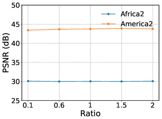
During the mask refinement stage, the mask is updated using the threshold ${\tau }_t$. To evaluate the influence of this parameter on cloud removal performance, experiments are conducted on the Africa 2 and America 2 datasets under Case3. Specifically, we set ${\tau }_t=\mathit{Ratio}\times {\tau }_t$ for validation. Figure 4 illustrates the PSNR variation curves of the proposed SCSSLR method on both datasets when the Ratio is set to 0.1, 0.6, 1, 1.5, and 2. The results show that PSNR values remain nearly unchanged as the Ratio varies within this range, indicating that this parameter has little effect on cloud removal performance.

Figure 4. Comparison of PSNR results for different ${\tau }_t$.

The pseudo-code for the PAM-based solving algorithm, designed for the SCSSLR-based thick cloud removal model, is presented in Algorithm 1. And we stop Algorithm 1 if

$${\displaystyle \frac{{∥{\mathcal{X}}^{(t+1)}-{\mathcal{X}}^{\left(t\right)}∥}_F}{{∥{\mathcal{X}}^{\left(t\right)}∥}_F}}<{10}^{-4},$$

holds or if the number of iterations reaches the maximum of 1000.

Algorithm 1 PAM-based algorithm for the thick cloud removal model

Input: The observed MTRSI $\mathcal{O}\in {\mathbb{R}}^{M\times N\times B\times T}$, the initial mask $\mathcal{M}$, the maximal FCTN-rank ${\mathit{r}}^{max}=\left(r_{12}^{max},r_{13}^{max},r_{14}^{max},r_{23}^{max},r_{24}^{max},r_{34}^{max}\right)$, the subspace dimension K, and the proximal parameter $\rho$. Initialization: the FCTN-rank $\mathit{r}=(1,1,1,1,1,1)$, ${\mathcal{G}}_1=rand(M,r_{12},$$r_{13},r_{14}),$${\mathcal{G}}_2=rand(r_{12},N,r_{23},r_{24})$, ${\mathcal{G}}_3=rand(r_{13},r_{23},K,r_{34}),{\mathcal{G}}_4=$$rand(r_{14},r_{24},$$r_{34},T)$, ${\left({\mathcal{A}}^t\right)}_{\left(3\right)}=\mathit{U}(:,1,:,K)$ and ${\mathit{F}}_t=\mathit{V}(1,:,K,:)$, where $\mathit{U}\mathit{S}\mathit{V}=SVD\left({\mathit{O}}_{\left(t\right)}\right)$, for $t=1,2,\cdots ,T$. while not converged and $t<t^{max}$ do     Update $\mathcal{Z}$ via (1), (2) and (3).     Update ${\mathit{F}}_{1:T}$ via (10).     Update $\mathcal{A}$ via (13).     Update ${\mathcal{G}}_{1:4}$ via (15).     Update $\mathcal{X}$ via (19).     Update $\mathcal{M}$ via (20).     Check the convergence condition:       ${∥{\mathcal{X}}^{(t+1)}-{\mathcal{X}}^{\left(t\right)}∥}_F/{∥{\mathcal{X}}^{\left(t\right)}∥}_F<{10}^{-4}$.     Let $\mathit{r}=min\left\{\mathit{r}+\right.$ ones $\left.(1,6),{\mathit{r}}^{max}\right\}$ and expand $\mathcal{G}$. end while Output: The restored MTRSI $\mathcal{X}$.

2.5. Computational Complexity

We analyze the computational complexity of SCSSLR. Let $\mathcal{O}\in {\mathbb{R}}^{M\times N\times B\times T}$ be the observed MTRSI, with subspace dimension $K<B$. Let $r_1$ and $r_2$ denote the maximal FCTN ranks in the subspace and original domains, respectively. The updates of $\mathcal{Z}$, $\mathcal{F}$, $\mathcal{A}$, ${\mathcal{G}}_{1:4}$, $\mathcal{X}$, and $\mathcal{M}$ yield the total cost $O\left((NKT+MKT+MNT+MNK)r_1^6+MNKT{r}_1^3+MNBKT\right).$ For comparison, the standard FCTN decomposition has complexity $O\left((NKT+MKT+MNT+MNK)r_2^6+MNKT{r}_2^3\right).$ Since $K<B$ and $r_1<r_2$, the dominant term in SCSSLR is strictly smaller than that of the original FCTN, indicating a lower overall computational cost.

3. Results

This section evaluates the performance of the proposed SCSSLR method on both simulated and real-world multitemporal remote sensing images. We compare the proposed method with ten representative baseline methods. The implementation details of all baseline methods, including code sources and parameter settings, are summarized in Table 5. For a fair comparison, all methods are implemented using the authors’ released codes, and their parameters are tuned according to the recommendations in the original papers. The pixel values of the test images are normalized to the range [0, 1] for each spectral band and each time node. All our computational results are obtained by running MATLAB 2018b with NVIDIA GeForce GTX 1050Ti 4GB.

Table 5. Baseline methods and implementation details.

Method	Parameters
TRTV [29]	TR rank and $\lambda$ adjusted as needed
TVLRSDC [30]	${\lambda }_1$, ${\lambda }_2$ and ${\lambda }_3$ adjusted as needed
FCTN [20]	FCTN rank adjusted as needed
SSTC-CR [28]	FCTN rank and K adjusted as needed
RCTVCR [9]	r and $\tau$ adjusted as needed
LRRSSN [31]	${\lambda }_2$ in the interval $[0.1,0.7]$
STLR-DP [32]	According to the original paper
L0-TC [22]	According to the original paper
OTNN [21]	According to the original paper
HNN [14]	According to the original paper

3.1. Simulated Experiments

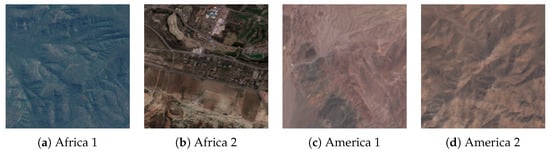
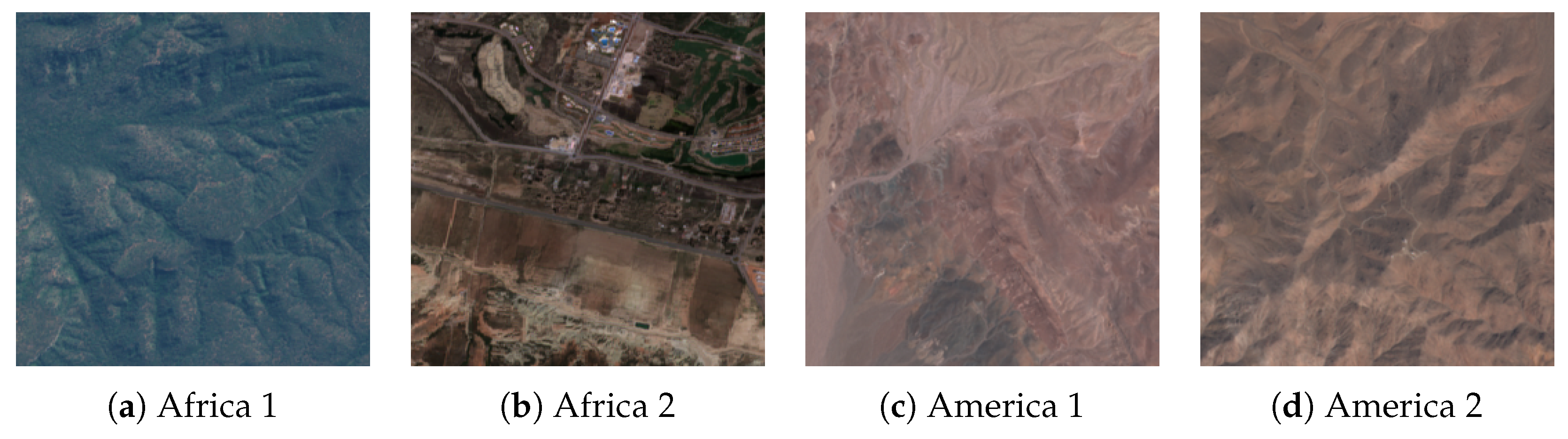
To evaluate the performance of the SCSSLR method, we utilize multitemporal remote sensing images from four datasets. These datasets named Africa 1, Africa 2, America 1 and America 2 [35]. Details of the datasets used for simulated experiments are provided in Table 6 and Figure 5.

Table 6. Four different MTRSIs in the simulated experiments.

Dataset	Spatial Size	Spectral Number	Time Node
Africa 1	256 × 256	13 (B1 to B13)	5
Africa 2	256 × 256	13 (B1 to B13)	6
America 1	256 × 256	13 (B1 to B13)	5
America 2	256 × 256	13 (B1 to B13)	6

Figure 5. Pseudo color images (R: B4, G: B3, and B: B2) of the four datasets.

For each test image, we simulate cloud coverage by assuming that clouds appear in the same spatial locations across all spectral bands at a given time node. We set all images at each time node to be affected by clouds for each test case. In this simulated experiment, a series of cloud masks with varying shapes and coverage levels were designed as presented in Table 7. The visual representation is based on $1-\mathcal{M}$, where white areas correspond to dense cloud regions, and black areas indicate cloud-free zones. Specifically, Case 1 features a cloud coverage between 22% and 36%. Case 2 exhibits cloud coverage ranging from 22% to 31%. Case 3 represents the level of cloud coverage with values ranging from 20% to 26%.

Table 7. Simulated masks for cloud mask completion experiments.

Case	Simulated Masks
Case 1
Case 2
Case 3

To assess the quality of the reconstructed image $\mathcal{X}\in {\mathbb{R}}^{M\times N\times B\times T}$ obtained from various methods, we utilize three quantitative evaluation metrics: peak signal-to-noise ratio (PSNR), structural similarity index (SSIM) [36], spectral angle mapping (SAM) [37] and correlation coefficient (CC) [38]. For the quantitative metrics, such as PSNR, SSIM, and CC, higher values indicate better image recovery, while for the SAM metric, lower values are preferred for better recovered images.

Table 8 summarizes the quantitative results on the Africa 1 and America 1 datasets under Case 1. Overall, HNN and SCSSLR achieve the best reconstruction performance. On America 1, HNN leverages the multi-scale representation of the wavelet transform to enhance structural and detail recovery, achieving a PSNR above 51 dB and outperforming all competing methods. SCSSLR ranks second, with a PSNR of 47.44 dB, still markedly superior to classical approaches such as TRTV and STLR-DP. Regarding computational cost, RCTVCR is the fastest method with a runtime of 0.071 s. Although SCSSLR requires 95.34 s, it remains significantly more efficient than traditional tensor- and sparsity-based methods, exemplified by STLR-DP with 1076 s, demonstrating a favorable balance between accuracy and efficiency.

Table 8. A quantitative evaluation of various methods under Case 1. The best result is highlighted in bold.

Data	Metric	Observed	TRTV	TVLRSDC	FCTN	SSTC-CR	RCTVCR	LRRSSN	STLR-DP	L0-TC	OTNN	HNN	SCSSLR
Africa 1	PSNR	8.556	37.71	24.33	36.68	41.94	31.03	37.64	42.71	38.91	41.62	44.70	42.58
	SSIM	0.725	0.917	0.843	0.904	0.972	0.915	0.931	0.972	0.952	0.973	0.983	0.974
	SAM	8.236	1.315	12.70	1.428	0.826	2.815	1.135	0.862	1.557	0.824	0.613	0.811
	CC	0.146	0.926	0.522	0.908	0.960	0.822	0.897	0.964	0.898	0.966	0.980	0.966
	Time	-	137.4	200.8	118.1	41.93	0.073	6401	1200	11.58	239.0	32.66	425.1
America 1	PSNR	12.10	39.58	38.81	38.00	46.96	32.75	40.03	37.72	41.98	46.05	51.07	47.44
	SSIM	0.821	0.958	0.968	0.934	0.982	0.942	0.970	0.959	0.977	0.980	0.995	0.988
	SAM	4.675	1.262	1.228	0.618	0.287	1.767	0.986	0.472	0.664	0.534	0.102	0.280
	CC	0.206	0.937	0.892	0.930	0.989	0.874	0.911	0.943	0.970	0.986	0.992	0.990
	Time	-	139.6	160.3	48.58	46.63	0.071	5804	1076	419.8	236.6	29.30	95.34

Table 9 presents the quantitative evaluation of various methods under Case 2 using precise masks, with the best results highlighted in bold. The results demonstrate that the proposed SCSSLR method exhibits superior reconstruction performance across both Africa 2 and America 2 datasets. Specifically, SCSSLR achieves the best scores across all four metrics for Africa 2. For the America 2 dataset, SCSSLR consistently maintains the leading position in terms of PSNR (44.60 dB) and CC (0.985), while delivering highly competitive results on SSIM and SAM compared with HNN and OTNN, respectively.

Table 9. A quantitative evaluation of various methods under Case 2. The best result is highlighted in bold.

Data	Metric	Observed	TRTV	TVLRSDC	FCTN	SSTC-CR	RCTVCR	LRRSSN	STLR-DP	L0-TC	OTNN	HNN	SCSSLR
Africa 2	PSNR	11.25	27.33	23.37	26.85	29.39	25.03	25.42	23.81	25.86	29.28	28.09	29.52
	SSIM	0.789	0.869	0.851	0.863	0.906	0.861	0.857	0.830	0.896	0.927	0.912	0.928
	SAM	3.792	1.854	6.900	1.812	1.725	5.304	6.074	2.362	2.343	1.392	1.479	1.289
	CC	0.360	0.944	0.841	0.938	0.962	0.881	0.852	0.877	0.924	0.965	0.954	0.967
America 2	PSNR	10.83	37.13	34.48	41.63	44.19	38.82	36.07	40.75	41.96	43.69	36.73	44.60
	SSIM	0.793	0.943	0.957	0.970	0.986	0.956	0.948	0.987	0.981	0.989	0.992	0.991
	SAM	5.694	0.382	1.653	0.307	0.248	1.423	1.273	0.218	0.369	0.167	0.241	0.244
	CC	0.125	0.922	0.847	0.968	0.979	0.876	0.869	0.924	0.964	0.983	0.931	0.985

Table 10 presents the quantitative evaluation of various comparison methods on the Africa 2 and America 2 datasets under Case 3, where the optimal indicators are highlighted in bold. The experimental results indicate that the proposed SCSSLR method demonstrates highly competitive performance. Specifically, SCSSLR achieves the highest PSNR value of 30.09 dB on the Africa 2 dataset, proving its superiority in restoring image brightness and contrast. In the America 2 dataset, its performance metrics remain at the forefront, ranking second only to HNN. Overall, while HNN holds a slight advantage in certain spectral fidelities, SAM, and structural similarity SSIM indicators, SCSSLR maintains a robust balance between reconstruction quality and spectral accuracy, thereby validating the effectiveness of the proposed algorithm.

Table 10. A quantitative evaluation of various methods under Case 3. The best result is highlighted in bold.

Data	Metric	Observed	TRTV	TVLRSDC	FCTN	SSTC-CR	RCTVCR	LRRSSN	STLR-DP	L0-TC	OTNN	HNN	SCSSLR
Africa 2	PSNR	11.56	27.33	23.57	27.05	30.00	27.35	28.03	24.67	27.59	29.85	30.07	30.09
	SSIM	0.791	0.871	0.855	0.869	0.909	0.899	0.878	0.845	0.900	0.929	0.986	0.911
	SAM	3.684	1.801	4.384	1.840	2.412	2.263	2.279	2.268	2.203	1.358	1.030	1.682
	CC	0.391	0.943	0.854	0.940	0.960	0.937	0.897	0.891	0.939	0.966	0.961	0.963
America 2	PSNR	12.37	36.97	34.79	41.87	43.47	34.88	35.26	30.87	41.60	43.03	45.79	44.01
	SSIM	0.818	0.947	0.957	0.971	0.987	0.957	0.946	0.929	0.981	0.988	0.993	0.989
	SAM	4.226	0.354	1.844	0.300	0.218	1.024	1.237	1.756	0.353	0.161	0.127	0.217
	CC	0.215	0.928	0.854	0.973	0.981	0.890	0.883	0.968	0.971	0.983	0.990	0.984

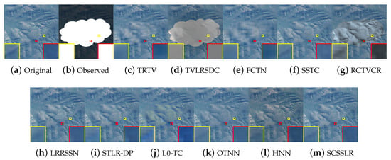
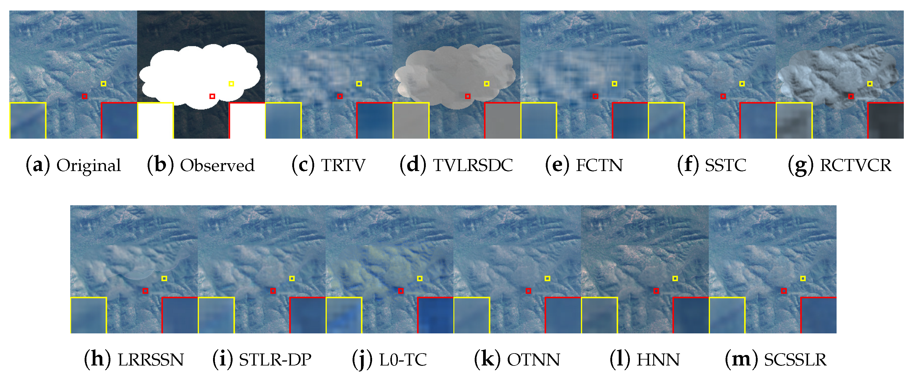
Figure 6 compares the reconstructed color images of different methods. SCSSLR produces results that are visually closest to the ground truth, effectively removing thick clouds, suppressing color distortions, and preserving physically plausible structures by exploiting spatial–spectral–temporal correlations. In contrast, TVLRSDC and RCTVCR fail to eliminate dense clouds, while TRTV, FCTN, and L0-TC introduce blurring and false color artifacts. Although HNN can remove cloud-covered regions, it suffers from noticeable pseudo-color distortions due to unfolding the original fourth-order tensor into a third-order form, which disrupts the intrinsic data structure. Enlarged regions further show that STLR-DP and OTNN oversmooth fine details, whereas LRRSSN retains edge artifacts. These results confirm that the integration of spatial–spectral low-rank constraints and Sobel-consistency enables SCSSLR to achieve superior restoration quality, especially in edge preservation.

Figure 6. Visual results of all comparison methods on the Africa 1 dataset at $t=2$. Each image is highlighted with a blue frame for clarity.

Figure 7 presents the restoration results on the Africa 2 dataset. SCSSLR produces reconstructions that are most consistent with the ground truth, effectively removing thick clouds while preserving fine details and sharp edges. As observed from the locally enlarged regions highlighted by the yellow boxes, competing methods still exhibit noticeable boundary artifacts and edge distortions. In contrast, the proposed method significantly suppresses such artifacts, which can be attributed to the edge-consistency constraint based on the Sobel convolution operator.

Figure 7. Visual results of all comparison methods on the Africa 2 dataset at $t=3$.

Figure 8 presents a visual comparison with enlarged regions highlighted by red boxes. TRTV, FCTN, and OTNN fail to recover the linear structures within the highlighted areas, indicating limited capability in preserving fine structural details. TVLRSDC, STLR-DP, and L0-TC suffer from noticeable boundary artifacts and color distortions. Although HNN is able to reconstruct major structures, it still exhibits inferior texture fidelity and color deviations. In contrast, SCSSLR not only better preserves fine texture details and edge structures but also maintains color appearances that are much closer to the ground truth. This superior performance can be attributed to the joint exploitation of guided feature-domain fidelity and Sobel-based consistency constraints.

Figure 8. Visual results of all comparison methods on the America 1 dataset at $t=2$.

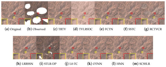
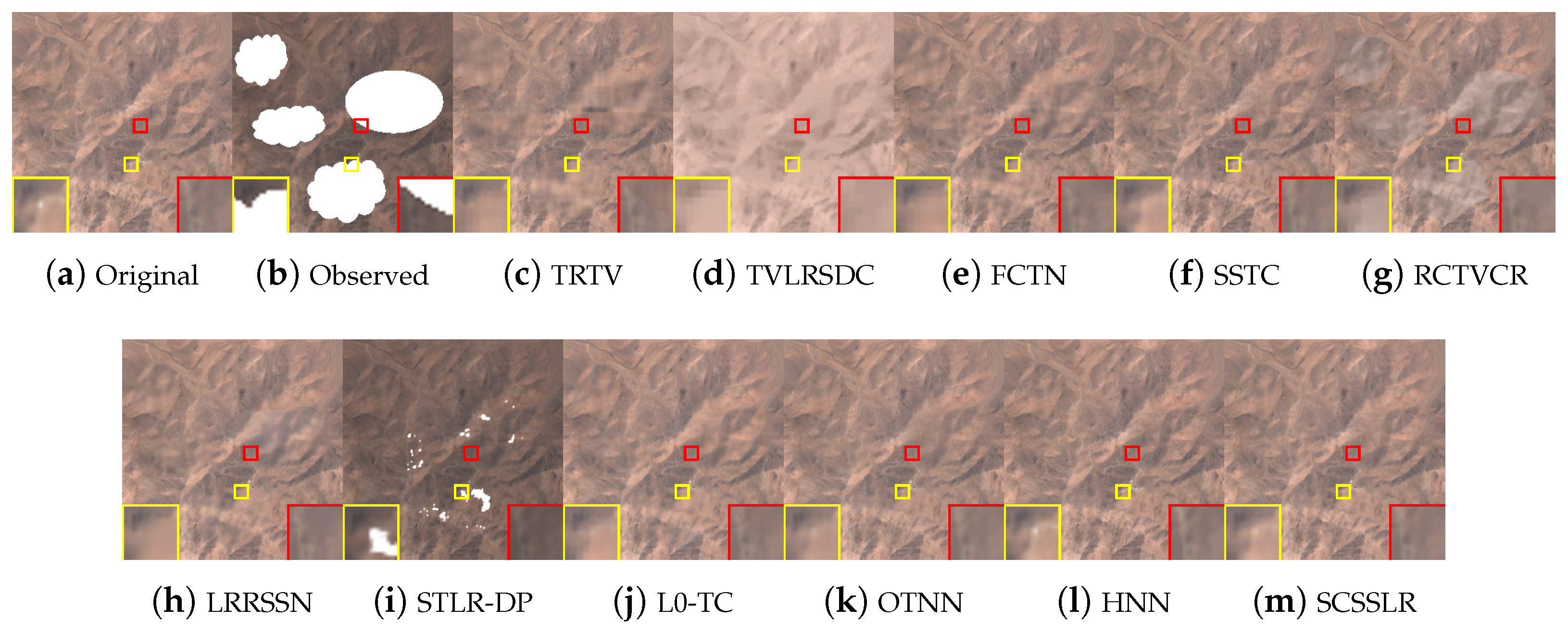
Figure 9 illustrates the Case 3 restoration results on the America 2 dataset, with enlarged subregions provided for clearer visual inspection. TVLRSDC suffers from severe color distortions, and FCTN introduces noticeable blurring, while TRTV, SSTC-CR, L0-TC, and OTNN fail to recover the white spot structures. STLR-DP is unable to completely remove thick cloud contamination, and RCTVCR and LRRSSN leave residual gray shadows. In contrast, SCSSLR effectively removes dense clouds and preserves fine structural details. As highlighted in the yellow boxed regions, the white spots restored by SCSSLR are noticeably clearer and more distinct, demonstrating its superior ability to recover subtle image details.

Figure 9. Visual results of all comparison methods on the America 2 dataset at $t=4$.

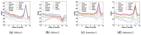
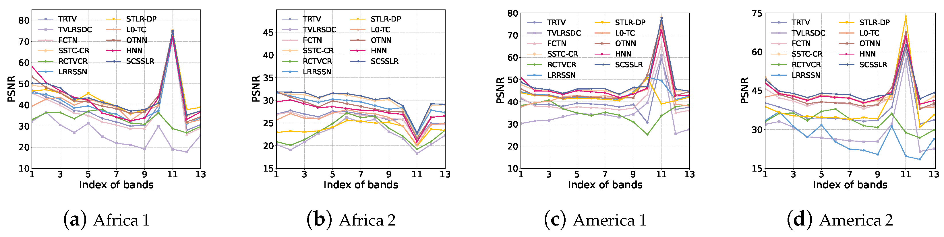
Figure 10 compares the PSNR curves of all competing methods across spectral bands and temporal frames for four representative datasets. For the Africa 2 dataset under Case 2, SCSSLR attains the highest PSNR over almost the entire spectral range, indicating strong spectral fidelity under severe cloud contamination. Similar behaviors are observed on Africa 1, America 1, and America 2, where SCSSLR consistently occupies the upper envelope of the PSNR curves. Although its PSNR is slightly lower than that of HNN at a few isolated bands, SCSSLR achieves superior performance in the majority of bands, demonstrating robust and stable reconstruction capability across diverse spatial–temporal scenarios.

Figure 10. Comparison of PSNR values across spectral bands at fixed temporal nodes for different datasets and competing methods.

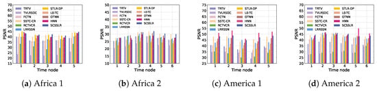
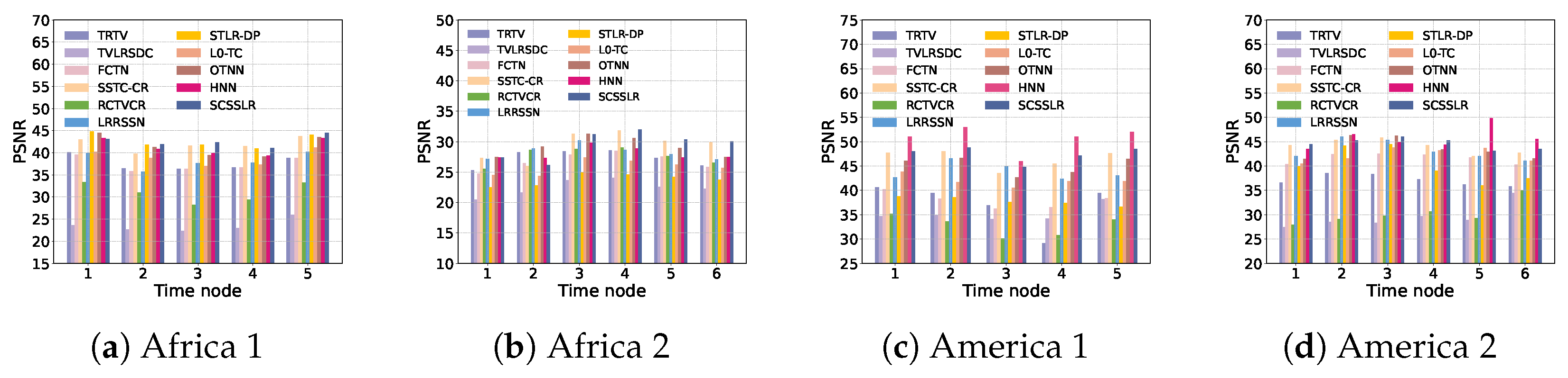
Figure 11 illustrates the average PSNR over spectral bands at different temporal nodes for all competing methods. On the Africa datasets, the proposed SCSSLR consistently achieves superior performance, delivering the highest or near-highest PSNR across most temporal nodes. For the America 1 dataset, HNN clearly outperforms the other methods and attains the best reconstruction accuracy. In contrast, on the America 2 dataset, SCSSLR achieves the highest PSNR in most temporal nodes, demonstrating its strong robustness under this scenario.

Figure 11. Comparison of average PSNR values across spectral bands at different temporal nodes for different datasets.

3.2. Real Experiments

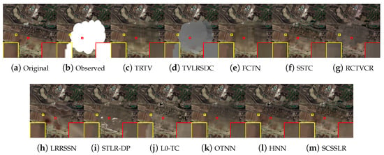
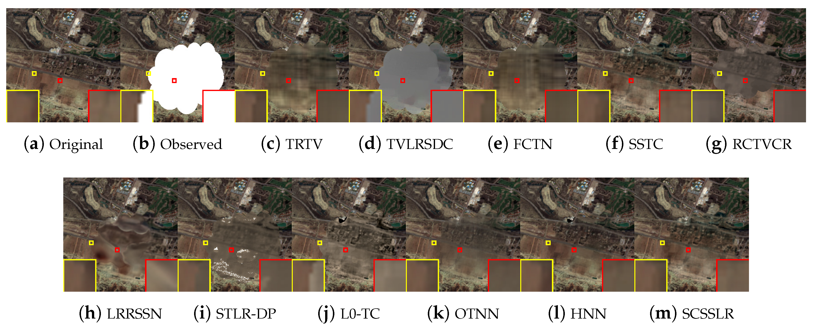
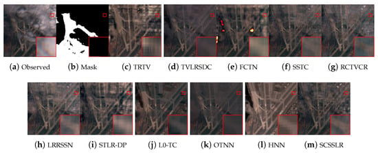
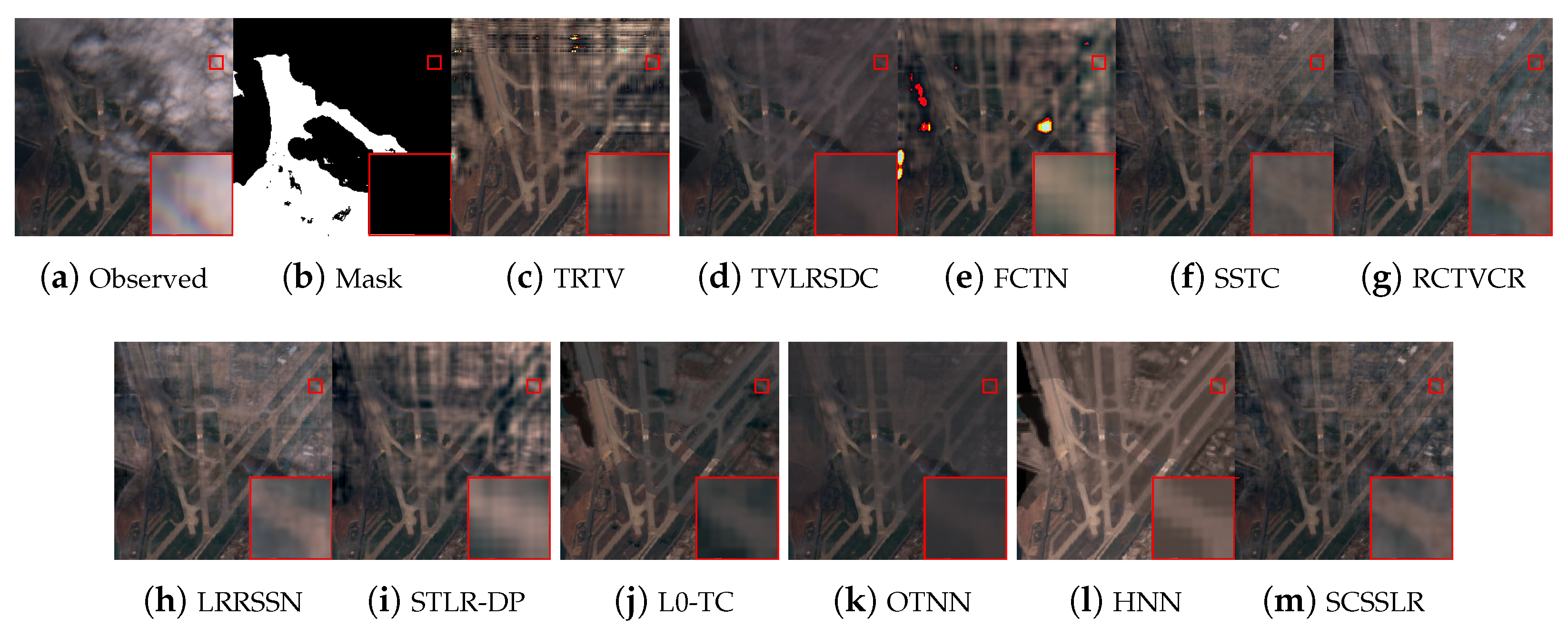
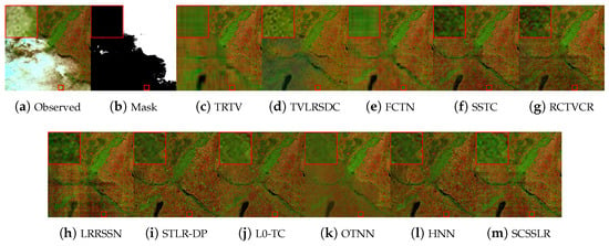
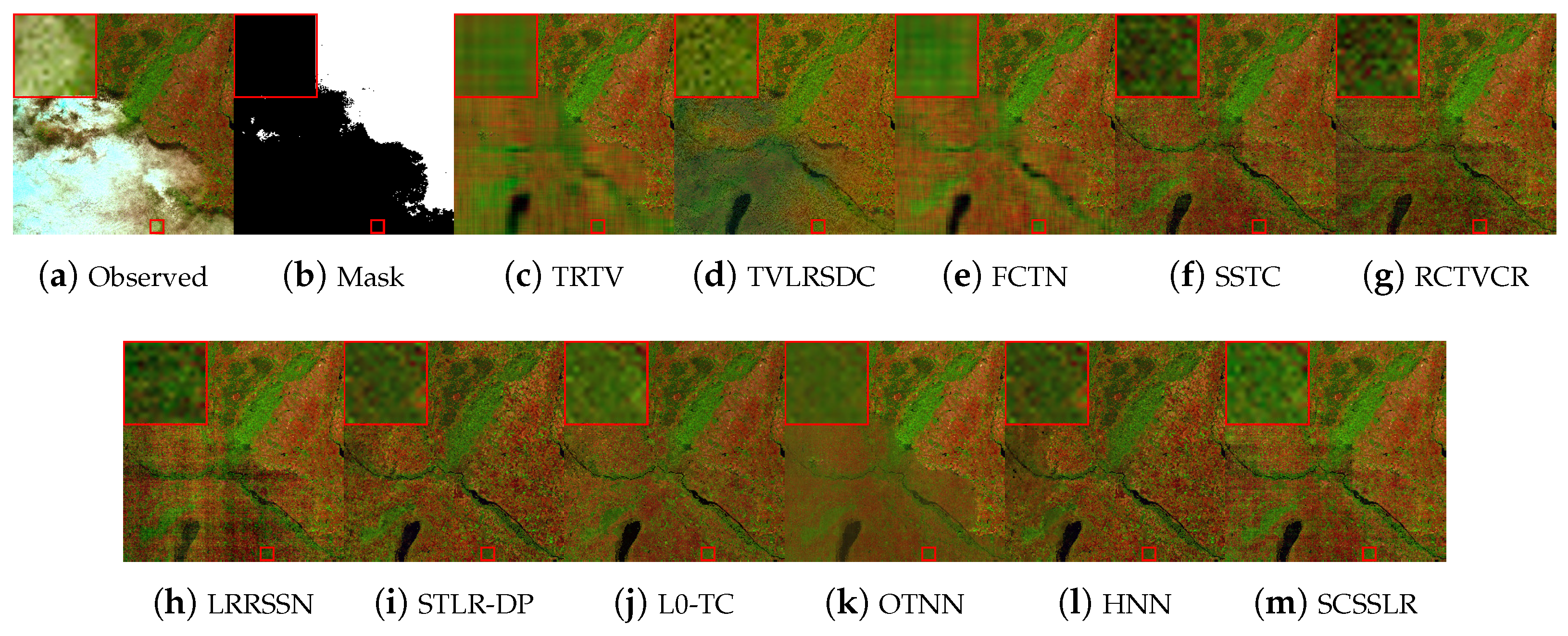
To further assess the effectiveness of the proposed SCSSLR method, experiments were conducted on two real-world datasets. The first dataset (Road), extracted from the SEM12MS-CR-TS collection, has dimensions $256\times 256\times 13\times 4$, where two temporal frames contain heavy clouds and shadows (Figure 12a). Since comparison methods require cloud masks, a mask covering all cloudy and shadowed areas is provided (Figure 12b). As shown in Figure 12, TRTV introduces boundary ringing, TVLRSDC fails to remove thick clouds, and FCTN struggles with large-scale occlusions. L0-TC, SSTC-CR, RCTVCR, LRRSSN, and OTNN are able to suppress cloud contamination but introduce shadow artifacts and suffer from boundary detail loss, while STLR-DP still leaves noticeable artifacts. HNN effectively removes thick clouds; however, it exhibits evident color distortions in the reconstructed regions. In contrast, SCSSLR preserves fine structures, eliminates visual artifacts, and reconstructs cloud-covered areas with brightness gradients that are consistent with those of the clear regions.

Figure 12. Visual results of all comparison methods on the Real1 dataset at $t=4$.

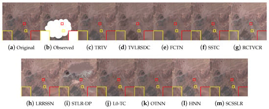
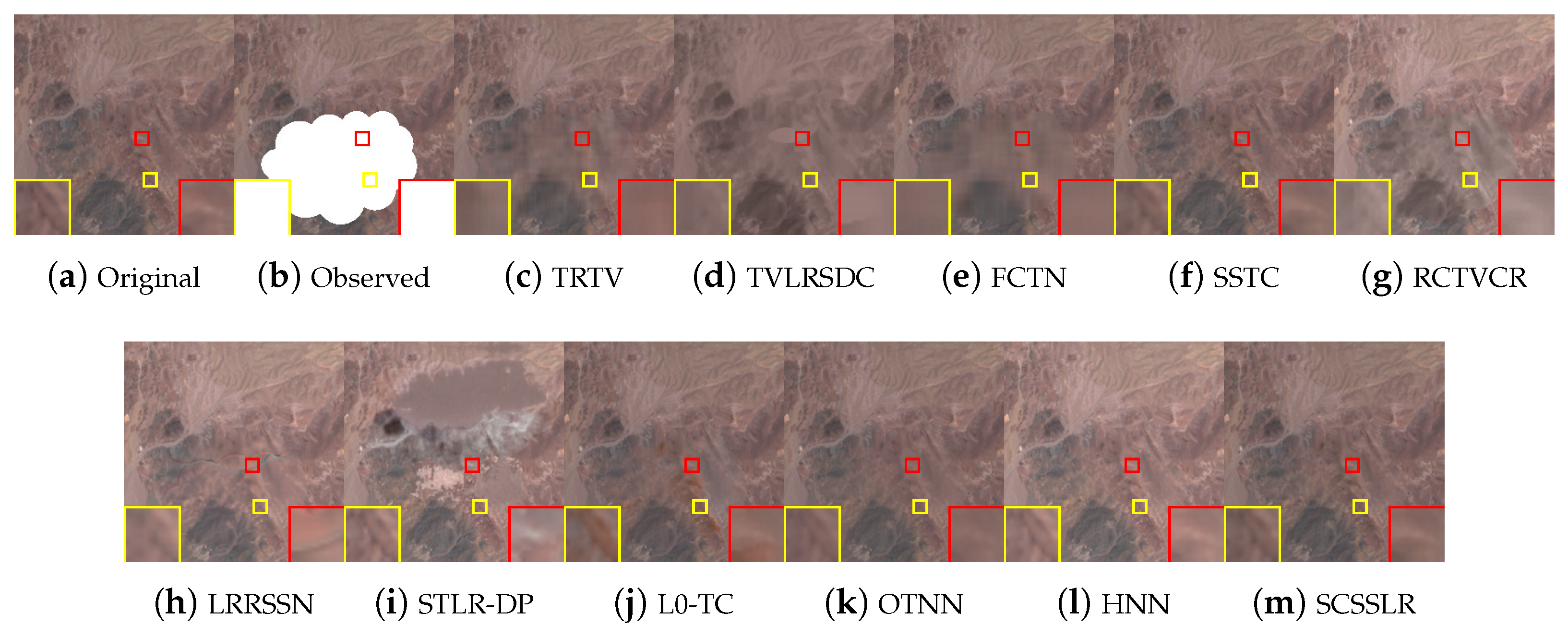
The second real dataset is derived from Sentinel-2B imagery [23], covering a $110\mathrm{km}\times 110\mathrm{km}$ area at 20 m resolution ($5490\times 5490$ pixels), details of the data are provided in Table 11. The data are normalized to [0, 1], and a cloud–shadow mask is provided for all methods. As shown in Figure 13, TRTV reduces cloud density but fails to recover the underlying scene, while FCTN can handle small dense clouds at the cost of noticeable color distortions. TVLRSDC, SSTC-CR, STLR-DP, L0-TC, and OTNN are able to suppress cloud contamination but suffer from overfitting artifacts, whereas RCTVCR and LRRSSN leave dark shadow residues. HNN successfully removes thick clouds; however, it leads to spectral inconsistencies and visible color deviations in the reconstructed regions. In contrast, SCSSLR produces clearer details and more faithful restorations by better preserving the intrinsic image structures and reinforcing spectral consistency, resulting in artifact-free reconstructions.

Table 11. Details of the multitemporal sequence images used in the real-data experiments.

Date	Satellite/Sensor	Field Size	Cloud Cover Ratio
16 August 2018	S2B	110 × 110 km (5490 × 5490)	14.76%
31 August 2018	S2A	$110\times 110$ km (5490 × 5490)	51.83%
5 September 2018	S2B	$110\times 110$ km (5490 × 5490)	10.97%
15 September 2018	S2B	$110\times 110$ km (5490 × 5490)	27.35%

Figure 13. Visual results of all comparison methods on the Real2 dataset at $t=4$.

3.3. Ablation Study

Ablation experiments are conducted on Africa 2 and America 2 (Case 3) to assess the roles of the spatiospectral low-rank (LR) prior and Sobel-consistency (SC). As shown in Table 12, removing either component (SCSSLR w/o LR or SCSSLR w/o SC) degrades performance, while the full SCSSLR consistently achieves the highest PSNR. SC notably improves dense-cloud removal, and the low-rank prior captures global spectral–temporal correlations, confirming their complementary contributions to SCSSLR’s superior performance.

Table 12. Results of PSNR analysis in ablation experiments on simulated datasets.The best result is highlighted in bold.

Model	Africa 2	America 2
SCSSLR w/o LR	27.56	39.03
SCSSLR w/o SC	29.44	43.04
SCSSLR	30.09	44.01

3.4. Comparison of Tensor Decompositions

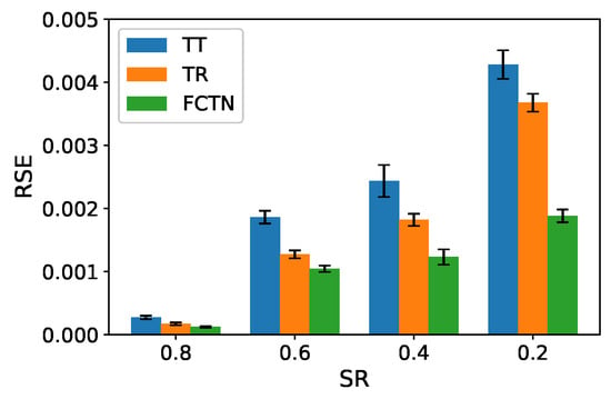
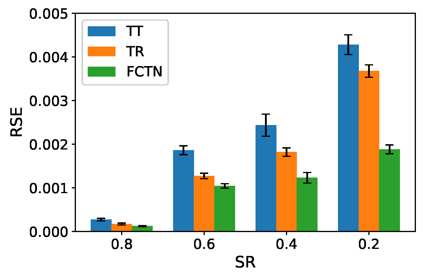
Furthermore, to verify the effectiveness of the adopted FCTN decomposition, we compare it with the TT and TR decompositions. Since cloud removal can be regarded as a tensor completion (TC) problem, controlled TC experiments are conducted on a synthetic fourth-order tensor of size $30\times 30\times 30\times 30$ with a predefined TT rank of $(20,100,20)$. The observed entries are uniformly sampled at sampling rates ranging (SR) from 0.2 to 0.8. For each sampling rate, the experiment is independently repeated 10 times using different random sampling patterns. The reconstruction performance is quantitatively evaluated by the relative squared error (RSE). Specifically, the mean RSE is computed by averaging the RSE values over all trials, while the corresponding Std is calculated to measure the variability across different random sampling realizations. The results are reported in the form of mean ± Std. As shown in Figure 14, the FCTN-based method consistently achieves the lowest mean RSE with a smaller standard deviation across all sampling rates. Specifically, when the sampling rate decreases from 0.8 to 0.2, the mean RSE of FCTN increases from approximately $1.2\times {10}^{-4}$ to $1.8\times {10}^{-3}$, while the corresponding standard deviations remain below $1.2\times {10}^{-4}$. In contrast, the TT-based method yields higher mean RSE values ranging from about $2.5\times {10}^{-4}$ to $4.3\times {10}^{-3}$, accompanied by noticeably larger standard deviations, whereas the TR-based method exhibits intermediate performance. These results indicate that the FCTN-based approach not only achieves superior reconstruction accuracy but also demonstrates higher robustness in modeling correlations among arbitrary mode pairs.

Figure 14. Comparison of RSE results for different decomposition methods in the TC problem.

4. Discussion

4.1. Parameter Analysis

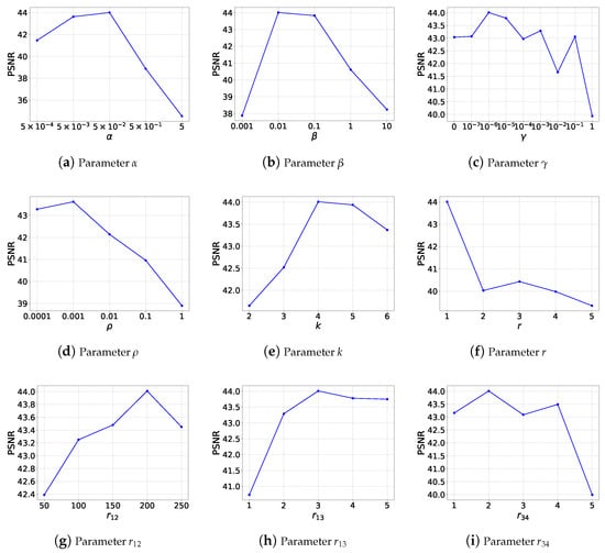
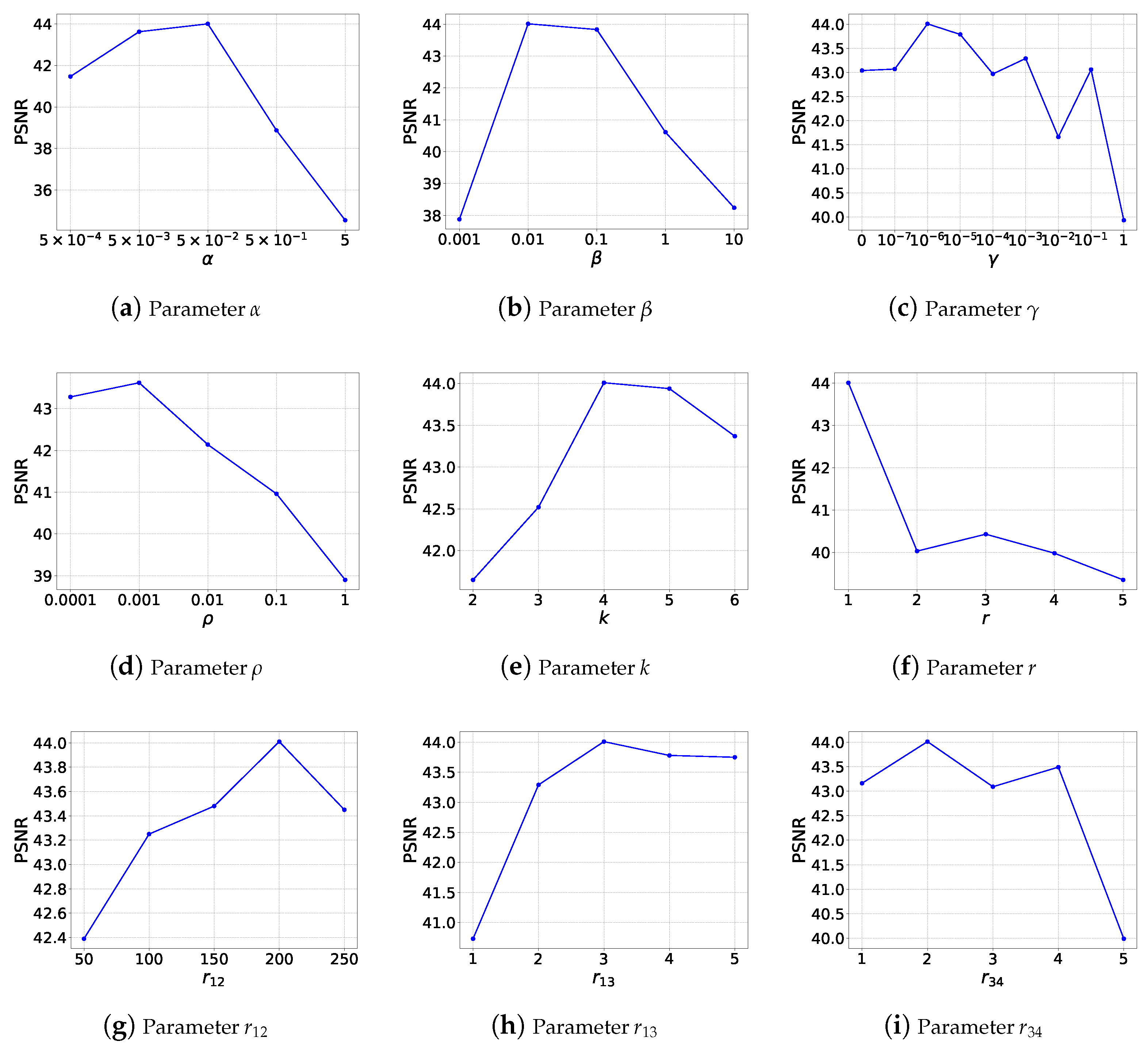
To analyze the influence of key parameters in SCSSLR, we evaluate the initial FCTN-rank $\mathit{r}$, subspace dimension K, and regularization/penalty parameters $\alpha$, $\beta$, $\gamma$, and $\rho$ using the America 2 dataset under Case 3. The maximal FCTN-rank is defined as $\mathit{r}=(r_{12},r_{13},r_{14},r_{23},r_{24},r_{34}),$ where $r_{13}$, $r_{14}$, $r_{23}$, and $r_{24}$ are set equal to reduce dimensionality. Thus, only $r_{12}$, $r_{13}$, and $r_{34}$ are tuned. The subspace dimension k is chosen from $\{2,3,\dots ,6\}$.

Figure 15 shows that SCSSLR achieves stable PSNR across a wide range of parameter settings. For $\alpha \in \{5\times {10}^{-4},{10}^{-3},5\times {10}^{-2},\dots ,5\}$, the highest PSNR occurs at $\alpha =5\times {10}^{-2}$ (Figure 15a). For $\beta \in \{0.001,0.01,0.1,1,10\}$, the optimal value is $\beta =0.001$ (Figure 15b). The parameter $\gamma$, varied over $\{0,{10}^{-7},{10}^{-6},{10}^{-5},\dots ,1\}$, shows moderate fluctuations (Figure 15c). For $\rho \in \{{10}^{-4},{10}^{-3},\dots ,1\}$, the best performance occurs at $\rho =0.001$ (Figure 15d). For the subspace dimension $K\in \{2,3,\dots ,6\}$, the peak PSNR is achieved at $K=4$, 5 (Figure 15e). The initial FCTN-rank $\mathit{r}\in \{1,2,3,4,5\}$ is tested, and $\mathit{r}=1$ gives the best performance (Figure 15f). To tune the major FCTN-rank components, we vary $r_{12}\in \{50,100,\dots ,250\},r_{13}\in \{1,2,3,4,5\},r_{34}\in \{1,2,3,4,5\}.$ As shown in Figure 15g,h, the optimal values are $r_{12}=200$, $r_{13}=3$, and $r_{34}=2$. Based on this analysis, the parameters used for all subsequent experiments are $\alpha =5\times {10}^{-2},\beta =0.001,K=4,r=1,r_{12}=200,r_{13}=3,r_{34}=2,$ while the parameter $\gamma$ is selected via grid search from the set $\{{10}^{-7},{10}^{-6},\dots ,{10}^{-1}\}$ with a logarithmic step of one order of magnitude.

Figure 15. Sensitivity analysis of model parameters on the America 2 dataset at $t=6$ under Case 3.

4.2. Convergence Analysis

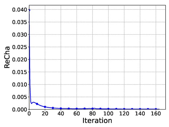
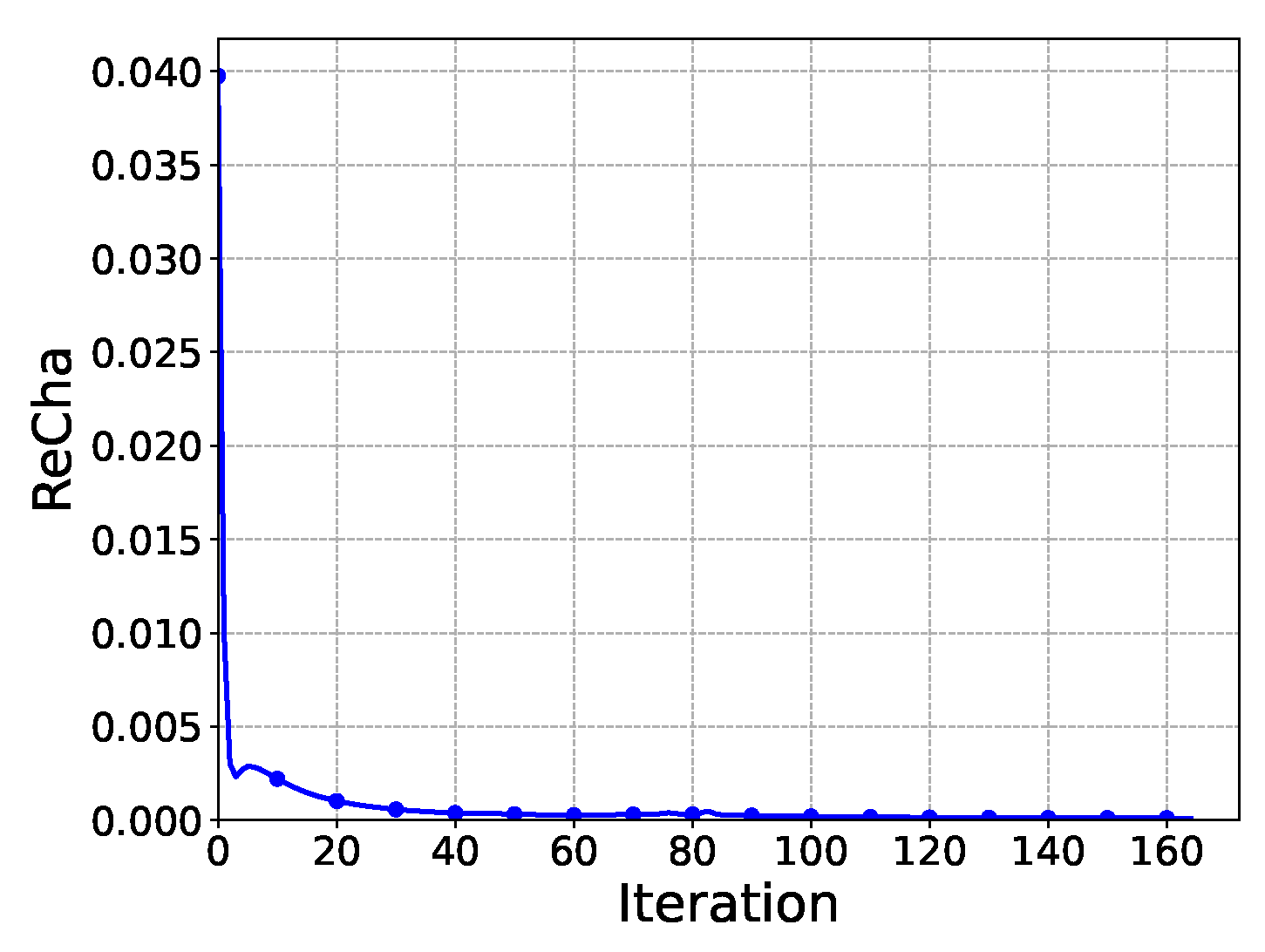
The convergence of the proposed PAM-based algorithm is assessed using the relative change $\mathrm{RelCha}={\displaystyle \frac{\parallel {\widehat{\mathcal{X}}}^{\left(t\right)}-{\widehat{\mathcal{X}}}^{(t+1)}{\parallel }_F}{\parallel {\widehat{\mathcal{X}}}^{\left(t\right)}{\parallel }_F}},$ where ${\widehat{\mathcal{X}}}^{\left(t\right)}$ is the reconstruction at iteration t. As shown in Figure 16, RelCha monotonically decreases and approaches zero for the America 2 dataset, indicating stable and reliable convergence of the proposed algorithm.

Figure 16. RelCha versus iteration number with America 2 dataset in Case3.

5. Conclusions

In summary, this study presents an effective framework for thick cloud removal in multitemporal remote sensing images based on Sobel-consistency and subspace-based spatiospectral low-rank tensor regularization. By exploiting the temporal consistency of edge structures, a Sobel-based edge regularization term is incorporated to improve the preservation of structural details and fine textures in cloud-covered regions. To further enhance data representation, a spectral-mode subspace projection is adopted to extract intrinsic spatiospectral components, leading to a compact and robust low-rank tensor formulation. Within this framework, spatial, spectral, and temporal correlations are jointly characterized using an FCTN model. An efficient PAM algorithm with progressive cloud mask refinement is developed to solve the proposed optimization problem. Extensive experiments on both simulated and real-world datasets demonstrate that the proposed method achieves consistently superior reconstruction performance and robustness compared with several state-of-the-art cloud removal approaches, particularly under heavy cloud coverage conditions.

Despite its strong performance, the framework remains computationally demanding. Future work may focus on lightweight approximations, adaptive rank selection, and deep learning acceleration, as well as extending the model to multi-source data and extreme weather for broader applicability.

References

- Luo, Y.S.; Zhao, X.L.; Jiang, T.X.; Chang, Y.; Ng, M.K.; Li, C. Self-Supervised Nonlinear Transform-Based Tensor Nuclear Norm for Multi-Dimensional Image Recovery. IEEE Trans. Image Process. 2022, 31, 3793–3808. [Google Scholar] [CrossRef] [Scilit] [PubMed]
- Zhao, D.; Zhong, W.; Ge, M.; Jiang, W.; Zhu, X.; Arun, P.V.; Zhou, H. SiamBSI: Hyperspectral video tracker based on band correlation grouping and spatial–spectral information interaction. Infrared Phys. Technol. 2025, 151, 106063. [Google Scholar] [CrossRef] [Scilit]
- Xiao, B.; Li, H.C.; Wang, R.; Zheng, Y.B. Fully-connected tensor network decomposition with gradient factors regularization for robust tensor completion. Signal Process. 2025, 233, 109933. [Google Scholar] [CrossRef] [Scilit]
- Zhu, Z.Y.; Huang, T.Z.; Huang, J.; Wu, L. Tensor singular value decomposition and low-rank representation for hyperspectral image unmixing. Signal Process. 2025, 230, 109799. [Google Scholar] [CrossRef] [Scilit]
- Zhao, D.; Zhang, H.; Arun, P.V.; Jiao, C.; Zhou, H.; Xiang, P.; Cheng, K. SiamSTU: Hyperspectral video tracker based on spectral spatial angle mapping enhancement and state aware template update. Infrared Phys. Technol. 2025, 150, 105919. [Google Scholar] [CrossRef] [Scilit]
- Zhao, D.; Zhou, L.; Li, Y.; He, W.; Arun, P.V.; Zhu, X.; Hu, J. Visibility estimation via near-infrared bispectral real-time imaging in bad weather. Infrared Phys. Technol. 2024, 136, 105008. [Google Scholar] [CrossRef] [Scilit]
- Zhu, X.; Gao, F.; Liu, D.; Chen, J. A modified neighborhood similar pixel interpolator approach for removing thick clouds in Landsat images. IEEE Geosci. Remote Sens. Lett. 2011, 9, 521–525. [Google Scholar] [CrossRef] [Scilit]
- Zhao, D.; Tang, L.; Arun, P.V.; Asano, Y.; Zhang, L.; Xiong, Y.; Tao, X.; Hu, J. City-scale distance estimation via near-infrared trispectral light extinction in bad weather. Infrared Phys. Technol. 2023, 128, 104507. [Google Scholar] [CrossRef] [Scilit]
- Xu, S.; Wang, J.; Wang, J. Fast Thick Cloud Removal for Multi-Temporal Remote Sensing Imagery via Representation Coefficient Total Variation. Remote Sens. 2024, 16, 152. [Google Scholar] [CrossRef] [Scilit]
- Zhao, D.; Asano, Y.; Gu, L.; Sato, I.; Zhou, H. City-Scale Distance Sensing via Bispectral Light Extinction in Bad Weather. Remote Sens. 2020, 12, 1401. [Google Scholar] [CrossRef] [Scilit]
- Lv, H.; Wang, Y.; Shen, Y. An empirical and radiative transfer model based algorithm to remove thin clouds in visible bands. Remote Sens. Environ. 2016, 179, 183–195. [Google Scholar] [CrossRef] [Scilit]
- Xu, M.; Jia, X.; Pickering, M.; Jia, S. Thin cloud removal from optical remote sensing images using the noise-adjusted principal components transform. ISPRS J. Photogramm. Remote Sens. 2019, 149, 215–225. [Google Scholar] [CrossRef] [Scilit]
- Zhao, D.; Yan, W.; You, M.; Zhang, J.; Arun, P.V.; Jiao, C.; Wang, Q.; Zhou, H. Hyperspectral Anomaly Detection Based on Empirical Mode Decomposition and Local Weighted Contrast. IEEE Sensors J. 2024, 24, 33847–33861. [Google Scholar] [CrossRef] [Scilit]
- Xu, S.; Yu, C.; Peng, J.; Chen, S.; Cao, X.; Meng, D. Haar Nuclear Norms with Applications to Remote Sensing Imagery Restoration. IEEE Trans. Image Process. 2025, 34, 6879–6894. [Google Scholar] [CrossRef] [Scilit]
- Wang, L.; Wang, Q. Fast spatial-spectral random forests for thick cloud removal of hyperspectral images. Int. J. Appl. Earth Obs. Geoinf. 2022, 112, 102916. [Google Scholar] [CrossRef] [Scilit]
- Luo, X.; Rong, W.; Zhou, J. A spatial-spectral adaptive thin-cloud removal method based on slow feature analysis. Remote Sens. Lett. 2022, 13, 747–755. [Google Scholar] [CrossRef] [Scilit]
- Li, Y.; Zhang, Y.; Li, H. Hyperspectral Image Completion Using Fully-Connected Extended Tensor Network Decomposition and Total Variation. IEEE J. Sel. Top. Appl. Earth Obs. Remote Sens. 2025, 18, 7543–7558. [Google Scholar] [CrossRef] [Scilit]
- Chen, B.; Huang, B.; Chen, L.; Xu, B. Spatially and Temporally Weighted Regression: A Novel Method to Produce Continuous Cloud-Free Landsat Imagery. IEEE Trans. Geosci. Remote Sens. 2017, 55, 27–37. [Google Scholar] [CrossRef]
- Lin, C.H.; Lai, K.H.; Chen, Z.B.; Chen, J.Y. Patch-Based Information Reconstruction of Cloud-Contaminated Multitemporal Images. IEEE Trans. Geosci. Remote Sens. 2014, 52, 163–174. [Google Scholar] [CrossRef] [Scilit]
- Zheng, Y.B.; Huang, T.Z.; Zhao, X.L.; Zhao, Q.; Jiang, T.X. Fully-Connected Tensor Network Decomposition and Its Application to Higher-Order Tensor Completion. Proc. AAAI Conf. Artif. Intell. 2021, 35, 11071–11078. [Google Scholar] [CrossRef] [Scilit]
- Qiu, Y.; Zhou, G.; Wang, A.; Zhao, Q.; Xie, S. Balanced Unfolding Induced Tensor Nuclear Norms for High-Order Tensor Completion. IEEE Trans. Neural Netw. Learn. Syst. 2025, 36, 4724–4737. [Google Scholar] [CrossRef] [Scilit] [PubMed]
- Xiao, J.L.; Huang, T.Z.; Deng, L.J.; Dou, H.X. A novel ℓ0 minimization framework of tensor tubal rank and its multi-dimensional image completion application. Inverse Probl. Imaging 2024, 18, 1366–1389. [Google Scholar] [CrossRef] [Scilit]
- Zhang, Q.; Yuan, Q.; Li, J.; Li, Z.; Shen, H.; Zhang, L. Thick cloud and cloud shadow removal in multitemporal imagery using progressively spatio-temporal patch group deep learning. ISPRS J. Photogramm. Remote Sens. 2020, 162, 148–160. [Google Scholar] [CrossRef] [Scilit]
- Zhang, Q.; Yuan, Q.; Li, Z.; Sun, F.; Zhang, L. Combined deep prior with low-rank tensor SVD for thick cloud removal in multitemporal images. ISPRS J. Photogramm. Remote Sens. 2021, 177, 161–173. [Google Scholar] [CrossRef] [Scilit]
- Melgani, F. Contextual reconstruction of cloud-contaminated multitemporal multispectral images. IEEE Trans. Geosci. Remote Sens. 2006, 44, 442–455. [Google Scholar] [CrossRef] [Scilit]
- Wang, J.; Olsen, P.A.; Conn, A.R.; Lozano, A.C. Removing Clouds and Recovering Ground Observations in Satellite Image Sequences via Temporally Contiguous Robust Matrix Completion. In Proceedings of the IEEE Conference on Computer Vision and Pattern Recognition (CVPR), Las Vegas, NV, USA, 27–30 June 2016. [Google Scholar]
- Czerkawski, M.; Upadhyay, P.; Davison, C.; Werkmeister, A.; Cardona, J.; Atkinson, R.; Michie, C.; Andonovic, I.; Macdonald, M.; Tachtatzis, C. Deep Internal Learning for Inpainting of Cloud-Affected Regions in Satellite Imagery. Remote Sens. 2022, 14, 1342. [Google Scholar] [CrossRef] [Scilit]
- Zheng, W.J.; Zhao, X.L.; Zheng, Y.B.; Lin, J.; Zhuang, L.; Huang, T.Z. Spatial-spectral-temporal connective tensor network decomposition for thick cloud removal. ISPRS J. Photogramm. Remote Sens. 2023, 199, 182–194. [Google Scholar] [CrossRef] [Scilit]
- He, W.; Yokoya, N.; Yuan, L.; Zhao, Q. Remote Sensing Image Reconstruction Using Tensor Ring Completion and Total Variation. IEEE Trans. Geosci. Remote Sens. 2019, 57, 8998–9009. [Google Scholar] [CrossRef] [Scilit]
- Chen, Y.; He, W.; Yokoya, N.; Huang, T.Z. Blind cloud and cloud shadow removal of multitemporal images based on total variation regularized low-rank sparsity decomposition. ISPRS J. Photogramm. Remote Sens. 2019, 157, 93–107. [Google Scholar] [CrossRef] [Scilit]
- Chen, Y.; Chen, M.; He, W.; Zeng, J.; Huang, M.; Zheng, Y.B. Thick Cloud Removal in Multitemporal Remote Sensing Images via Low-Rank Regularized Self-Supervised Network. IEEE Trans. Geosci. Remote Sens. 2024, 62, 5506613. [Google Scholar] [CrossRef] [Scilit]
- Zou, Z.; Chen, L.; Jiang, X. Spectral–Temporal Low-Rank Regularization with Deep Prior for Thick Cloud Removal. IEEE Trans. Geosci. Remote Sens. 2024, 62, 5400916. [Google Scholar] [CrossRef] [Scilit]
- Li, L.Y.; Huang, T.Z.; Zheng, Y.B.; Zheng, W.J.; Lin, J.; Wu, G.C.; Zhao, X.L. Thick Cloud Removal for Multitemporal Remote Sensing Images: When Tensor Ring Decomposition Meets Gradient Domain Fidelity. IEEE Trans. Geosci. Remote Sens. 2023, 61, 5512414. [Google Scholar] [CrossRef] [Scilit]
- Lin, J.; Huang, T.Z.; Zhao, X.L.; Jiang, T.X.; Zhuang, L. A Tensor Subspace Representation-Based Method for Hyperspectral Image Denoising. IEEE Trans. Geosci. Remote Sens. 2021, 59, 7739–7757. [Google Scholar] [CrossRef] [Scilit]
- Ebel, P.; Xu, Y.; Schmitt, M.; Zhu, X.X. SEN12MS-CR-TS: A Remote-Sensing Data Set for Multimodal Multitemporal Cloud Removal. IEEE Trans. Geosci. Remote Sens. 2022, 60, 5222414. [Google Scholar] [CrossRef] [Scilit]
- Wang, Z.; Bovik, A.; Sheikh, H.; Simoncelli, E. Image quality assessment: From error visibility to structural similarity. IEEE Trans. Image Process. 2004, 13, 600–612. [Google Scholar] [CrossRef] [Scilit]
- Kruse, F.A.; Lefkoff, A.B.; Boardman, J.W.; Heidebrecht, K.B.; Shapiro, A.; Barloon, P.; Goetz, A.F. The spectral image processing system (SIPS)—Interactive visualization and analysis of imaging spectrometer data. Remote Sens. Environ. 1993, 44, 145–163. [Google Scholar] [CrossRef] [Scilit]
- Li, X.; Shen, H.; Zhang, L.; Zhang, H.; Yuan, Q.; Yang, G. Recovering Quantitative Remote Sensing Products Contaminated by Thick Clouds and Shadows Using Multitemporal Dictionary Learning. IEEE Trans. Geosci. Remote Sens. 2014, 52, 7086–7098. [Google Scholar] [CrossRef] [Scilit]
Disclaimer/Publisher’s Note: The statements, opinions and data contained in all publications are solely those of the individual author(s) and contributor(s) and not of MDPI and/or the editor(s). MDPI and/or the editor(s) disclaim responsibility for any injury to people or property resulting from any ideas, methods, instructions or products referred to in the content. |
© 2026 by the authors. Licensee MDPI, Basel, Switzerland. This article is an open access article distributed under the terms and conditions of the Creative Commons Attribution (CC BY) license.