Estimation and Analysis of Stokes Drift Based on CFOSAT Wave Spectrum Data

Highlights

What are the main findings?

• By introducing a wind-speed-dependent parameterization scheme for the transition wavenumber between the equilibrium and saturation ranges, as well as a cutoff wavenumber to supplement the high-frequency tail of the CFOSAT wave spectrum, the estimated Stokes drift shows a significant improvement.
• The contribution of high-frequency waves to Stokes drift exhibits pronounced spatial heterogeneity, exceeding 80% in equatorial low-wind regions while dropping below 10% in the high-wind Southern Ocean due to enhanced breaking dissipation.

What are the implications of the main findings?

• The high-frequency supplementation method proposed in this study outperforms the widely used ERA5 reanalysis, providing a more reliable data source for estimating global Stokes drift from satellite wave spectra; this can enhance applications such as trajectory prediction for floating marine debris.
• The findings reveal the global distribution and seasonal variability characteristics of Stokes drift and its high-frequency contribution, which can help improve the parameterization of upper-ocean mixing processes in climate models and advance the simulation of air–sea interactions and oceanic material transport.

Abstract

Stokes drift is the net displacement of ocean surface water particles caused by nonlinear surface waves. Its estimation typically relies on sea surface wave spectra, and truncation of the high-frequency spectral tail can significantly affect accuracy. This study uses directional wave spectrum data from the SWIM instrument onboard CFOSAT. By introducing a wind-speed-dependent parameterization scheme for the transition wavenumber (k_n) between the equilibrium and saturation ranges, as well as a cutoff wavenumber (k_m), we constructed a model to supplement the high-frequency tail of the wave spectrum combined with mask filtering to optimize spectrum reconstruction. The Stokes drift calculated with this model shows a better correlation (R = 0.699) with buoy observations than the widely used ERA5 reanalysis (R = 0.613). Analysis reveals pronounced regional differences in the contribution of high-frequency waves to surface Stokes drift, exceeding 80% in equatorial low-wind regions while dropping below 10% in the high-wind Southern Ocean due to enhanced breaking dissipation. The global Stokes drift distribution exhibits clear hemispheric asymmetry and seasonal evolution, with peak values (>0.12 m/s) in the Antarctic Circumpolar Current region. The proposed method provides a reliable, observation-based approach for improving global Stokes drift estimation, with direct implications for modelling ocean transport, Langmuir turbulence, and air–sea interactions.

1. Introduction

When surface gravity waves propagate in water, water particles do not merely execute closed orbital motions but experience a small net displacement in the direction of wave propagation. This long-term cumulative average displacement is known as Stokes drift. Stokes drift is defined as the difference between the mean Lagrangian particle motion in the wave field and the phase-averaged Eulerian velocity [1]. In practical applications, the calculation of Stokes drift is typically based on the lowest-order approximation of the Taylor-expanded Lagrangian trajectory.

Stokes drift plays a crucial role in the marine environment. Studies show that it accounts for approximately two-thirds of the wind-driven surface layer drift [2] and exhibits strong vertical shear [3,4]. This mechanism is widely applied in predicting the trajectories of floating objects (e.g., marine debris [5], microplastics [6], pollutant aggregation [7], and aircraft wreckage tracing [8]). Furthermore, Stokes drift significantly influences the transport of plankton eggs, larvae, and dissolved substances [9,10] and ecological isolation assessments [11]. In coastal zones, mass flux conservation induced by Stokes drift leads to offshore-directed bottom currents [12,13] and interacts with momentum input from wave breaking [14]. Simultaneously, Stokes drift modulates submesoscale fronts and filamentary structures [15,16].

The shear interaction between Stokes drift and the Eulerian mean current generates the Craik–Leibovich vortex force [17], driving Langmuir turbulence. This turbulence is a dominant mechanism for mixing and transport in the ocean surface boundary layer [18,19]. Additionally, the Coriolis effect associated with surface wave phase velocity produces the Stokes–Coriolis force [20,21], altering momentum distribution in the upper ocean (e.g., modifying the Ekman profile) and impacting hydrodynamic processes in both open and coastal regions [22,23]. In recent years, with the increasing application of artificial intelligence in ocean forecasting, the estimation of Stokes drift has also been incorporated into data-driven correction models. For instance, Garcia-Leon et al. [24] proposed a sub-inertial surface current correction method based on artificial neural networks, in which Stokes drift serves as one of the key covariates, significantly enhancing the accuracy of flow field forecasting. Furthermore, this study also utilized Sentinel-1 SAR data to correct coastal wind fields, facilitating a more precise distinction between wind waves and swells, thereby further optimizing the division of wave spectra. These advancements indicate that high-precision Stokes drift and wind field data are not only crucial for traditional physical models but also provide essential inputs for data assimilation and machine-learning-driven ocean forecasting. Therefore, developing reliable, observation-based Stokes drift estimation methods holds direct significance for enhancing the performance of wave spectrum analysis, drift prediction, and coupled forecasting systems.

Currently, the primary methods for obtaining wave spectra to compute Stokes drift can be categorized into three types: empirical wave spectra, wave spectra derived from remote sensing observations, and wave spectra simulated by numerical wave models. Each of these approaches has its own advantages and inherent limitations. The first method utilizes empirical wave spectra (e.g., the Pierson–Moskowitz or JONSWAP spectra), which are constructed based on a limited set of parameters such as wind speed. While computationally efficient and widely used in large-scale climate models, these parameterized spectra often oversimplify the complex reality of the sea state. They typically lack detailed directional information and fail to accurately represent the high-frequency tail of the spectrum, leading to significant uncertainties in Stokes drift estimates, particularly in complex wind–sea–swell mixed conditions [3,4]. The second method leverages remote sensing observations from satellites, such as altimeters and synthetic aperture radars (SAR). Instruments like the SWIM scatterometer on CFOSAT provide valuable two-dimensional wave spectrum data with global coverage. However, these spaceborne sensors are often limited in their ability to resolve high-frequency waves due to instrumental constraints like spatial resolution and signal-to-noise ratio. The inevitable truncation of the wave spectrum at higher wavenumbers results in an underestimation of Stokes drift, as high-frequency waves, despite their small amplitudes, contribute substantially to the net drift due to their large numbers [25]. The third method relies on numerical wave models (e.g., WAVEWATCH III), which assimilate various observations to simulate the evolution of the wave field. These models can provide spatially and temporally continuous wave spectra. Nevertheless, the accuracy of their Stokes drift products is contingent upon the model’s physical parameterizations, especially for the high-frequency spectral tail and wind input/dissipation sources, so deviations in the modeled spectra will lead to deviations in Stokes drift.

In recent years, scholars have realized that the contribution of high-frequency waves to the Stokes drift is not negligible [26] and that by neglecting the high-frequency contribution, the prediction of surface Stokes drift may be underestimated by more than 50% [25]. Therefore, all current methods face a key challenge in Stokes drift estimation, which is accurate measurement of the high-frequency part of the directional spectrum [27].

Advancements in remote sensing and in situ observation techniques have significantly enhanced the spatial and temporal resolution of waves in recent years. For instance, studies based on airborne lidar data have revealed the power-law characteristics of wavenumber spectra in the equilibrium and saturation ranges [28,29]. Phillips’ model predicts a (k^−5/2) slope for the equilibrium range of the omnidirectional wavenumber spectrum. Beyond the equilibrium range, spatial and temporal observations of the saturation range show a power-law transition of wavenumber from k^−5/2 to k⁻³ slope [28,30,31,32]. If it is the frequency spectrum of deep-water waves, the slope in the equilibrium range domain is f⁻⁴ and the slope in the saturation range domain is f⁻⁵. However, accurately capturing high-frequency wave spectra, particularly the transition segment between the equilibrium and saturation ranges, remains challenging. Lenain and Pizzo [25] characterized the properties of the surface wave field across these ranges and provided a simple parameterization model for the transition, which can easily be implemented in numerical wave models.

The accuracy of Stokes drift estimation is not only crucial for its own characterization but also serves as a key input for numerous marine and coastal applications. In coastal forecasting systems, Stokes drift is utilized to predict the transport trajectories of floating debris, assess coastal erosion risks, and simulate flood inundation during storm surges. However, the reliability of these applications fundamentally relies on the precision of input data for wind and wave fields. Studies have shown that under conditions of steep wind field gradients or extreme weather, even relatively small errors in wind and wave input data can be amplified in subsequent high-resolution coastal hydrodynamic–geomorphic dynamic simulations, leading to significant prediction biases [33]. Therefore, developing a more accurate Stokes drift estimation method based on direct observations is of great value in reducing source errors in such operational forecasting chains and enhancing their overall reliability. This study aims to utilize CFOSAT satellite observations to provide a more reliable observational benchmark for global Stokes drift estimation by improving the high-frequency part of its spectrum. The Surface Waves Investigation and Monitoring (SWIM) instrument onboard the China–France Oceanography Satellite (CFOSAT) provides wave spectra using its off-nadir beams. The instrument emits one vertical (0°) and five low-incidence-angle beams (2°, 4°, 6°, 8°, and 10°) and employs a rotating scanning method to acquire sea surface reflection and quasi-specular scattering information at different incidence angles [34]. Based on the modulation information of the scattering coefficient by multi-azimuth wave slopes, the directional wave spectrum can be retrieved, yielding wave parameters such as significant wave height (SWH) [35,36,37]. Although CFOSAT provides abundant observed wave spectra, its limited sensitivity to high-frequency waves hinders precise Stokes drift computation. Therefore, augmenting CFOSAT’s high-frequency spectral data is essential for improving drift predictions.

Therefore, to address the key issue of high-frequency spectral truncation in satellite observations, this study developed a wind-speed-dependent parameterization scheme based on CFOSAT spectral data to reconstruct the high-frequency spectral tail, thereby optimizing the estimation of global Stokes drift. The structure of this paper is organized as follows. Section 1 has introduced the phenomenon of Stokes drift, its oceanographic significance, and current estimation methodologies. Section 2 describes the datasets used, including CFOSAT, NDBC buoys, ERA5, and ETOPO2 bathymetry. Section 3 details the methodology, including mask filtering, spectral conversion and calibration, the high-frequency tail supplementation scheme, and Stokes drift calculations. Section 4 presents comparison results with buoys and ERA5 and analyzes the global distribution and seasonal variability in surface Stokes drift, Stokes transport and their high-frequency contributions. Finally, Section 5 summarizes the main conclusions and discusses the implications of our findings.

2. Materials and Methods

2.1. China–France Oceanography Satellite (CFOSAT)

The China–France Oceanography Satellite (CFOSAT) was jointly developed by the French National Centre for Space Studies (CNES, 18 Avenue Edouard Belin, 31400 Toulouse, France) and the China National Space Administration (CNSA, Beijing, China). Launched in October 2018, CFOSAT operates in a sun-synchronous orbit at an altitude of approximately 500 km, achieving global coverage every 13 days, with a maximum latitude reach of 82.56°. The distance between adjacent tracks is 200 km. Its mission is to deepen understanding of air–sea interactions through synchronous monitoring of global sea surface wind fields and wave fields [36]. The satellite carries two Ku-band (13.2–13.6 GHz) instruments: the SCATterometer (SCAT) and the Surface Wave Investigation and Monitoring (SWIM) instruments. The SCAT instrument was developed by the China Academy of Space Technology (CAST, Beijing, China). SWIM was developed by Thales Alenia Space (Cannes, France) in collaboration with the French National Centre for Space Studies (CNES, Toulouse, France). SCAT is used to retrieve wind vectors [38], while SWIM, as the first spaceborne real-aperture wave scatterometer, acquires two-dimensional wave spectrum data, supporting spectral analysis of wind waves, swells, and mixed seas [39].

SWIM continuously observes the sea surface using six incidence angles: 0°, 2°, 4°, 6°, 8°, and 10°. The nadir (0°) beam estimates significant wave height (SWH) using the radar altimeter principle. The 2° and 4° beams primarily supplement normalized radar cross-section information. The 6°, 8°, and 10° beams are responsible for retrieving the two-dimensional ocean wave spectrum, decomposed into 12 directional bins (0–180°, 15° interval) and 32 non-uniform wavenumber bins (k = 0.0126 rad/m to k_c = 0.2789 rad/m), corresponding to wavelengths of 70–500 m. The retrieved spectrum has a horizontal resolution of 70 × 90 km and is archived in the SWIM Level 2 product. This study selected spectral data from the SWIM 10° beam for Stokes drift estimation, based on recent systematic evaluations of SWIM L2 products and consistency analysis with other observation methods. Liang et al. [40] found that among all the beams (6°, 8°, 10°) in SWIM, the 10° beam showed the most stable inversion accuracy in terms of significant wave height and main wave direction, especially after the data processing algorithm update in June 2020, where its data consistency was further improved. In addition, Hao et al. [41] systematically evaluated the consistency of spectral parameters at different incident angles by comparing SWIM spectra with SWAN numerical simulation results and high-resolution SAR inversion spectra. Their research clearly indicates that the 10 ° beam exhibits the best comprehensive performance in multiple key parameters such as effective wave height, peak wavelength, and peak period: compared with SWAN simulation, its effective wave height has the lowest root mean square error (1.02 m) and the highest correlation coefficient (0.79); compared with SAR inversion spectra, the spectral shape and energy distribution of the 10° beam are closest to the SAR results, the correlation coefficient of which is 0.77. All studies have shown that the spectral inversion performance of the 10° beam is superior to these studies of the 6° and 8° beams [38,42]. Therefore, selecting the 10° beam with the best data quality for analysis can minimize the Stokes drift estimation bias caused by errors in the original spectrum, ensuring the reliability of the high-frequency supplementary method proposed in this study and the global drift analysis results.

For this study, we analyze directional slope spectrum data acquired by SWIM from 1 December 2022 to 1 December 2023. The relevant data are publicly available via [43].

2.2. NDBC Buoys

Buoy observation data are widely regarded as a relatively accurate reference standard for wave measurements and serve as crucial validation data for satellite remote sensing products. The buoy data used in this study are from the National Data Buoy Center (NDBC) in the Stennis Space Center, MS, United States, which operates the world’s largest network of wave buoys and provides open datasets, and some of these buoys directly provide observed wave frequency spectra. According to NDBC technical reports, wave frequency spectra are estimated by measuring the vertical displacement or heave acceleration of the buoy hull during wave sampling. Raw measurement data are converted from the time domain to the frequency domain using Fast Fourier Transform (FFT). The distortion caused by hull dynamics and electronic noise is then corrected using the Response Amplitude Operator (RAO), yielding the calibrated wave frequency spectrum [44].

The wave spectrum data provided by NDBC are hourly observations, containing key spectral analysis parameters such as omnidirectional spectral density, dominant wave direction, and mean wave direction. The frequency coverage ranges from 0.020 to 0.485 Hz, with 47 frequency bins at intervals of approximately 0.01 Hz [45]. The relevant data can be publicly accessed via the NDBC official website [46]. The buoy numbers, locations, and water depth characteristics selected in this article are shown in

Table 1. The buoy-related information used in this article.

Number	Latitude	Longitude	Water Depth Characteristics
41,010	28.878N	78.467W	shallow water
41,013	33.441N	77.764W	shallow water
41,040	14.536N	53.136W	deep water
41,049	27.505N	62.271W	deep water
42,002	25.950N	93.78W	deep water
42,060	16.434N	63.329W	deep water
44,011	41.088N	66.546W	shallow water
46,035	57.034N	177.468W	deep water
46,073	55.008N	172.012W	deep water
51,001	24.475N	162.03W	deep water

. The 10 NDBC buoys selected in this study have systematic representative significance in spatial distribution, water depth environment, and sea state types. These buoys cover the main basins of the Pacific, Atlantic, and Indian Oceans and can reflect different climate and wind wave systems from the equatorial low-wind zone to the mid- to high-latitude westerly belt. In terms of water depth types, it includes deep-water buoys such as 46,035 and 51,001, located in open oceans, whose spectra are less affected by seabed topography and are suitable for testing the observation performance of satellites in pure sea conditions. It also includes buoys such as 41,013 and 44,011 located in shallow waters, which have complex spectral structures due to nearshore topography, wave reflection and refraction, and can be used to evaluate the robustness of CFOSAT spectral processing technology in complex sea conditions. The selected buoys also cover various wave systems such as wind-wave-dominant, swell-dominant, and mixed sea conditions, which helps to comprehensively verify the applicability of the wind-speed-dependent high-frequency supplementary parameterization scheme proposed in this study in different geographical distributions and dynamic environments.

2.3. ERA5

ERA5 is the fifth-generation global atmospheric reanalysis dataset released by the European Centre for Medium-Range Weather Forecasts (ECMWF, Shinfield Park, Reading, RG2 9AX, UK). It provides hourly historical and near-real-time data from 1950 to the present, with a time resolution of 1 h and a spatial resolution of 31 km, covering key atmospheric and ocean wave parameters. Its wind field data are obtained via the Climate Data Store, with the highest spatial resolution being 0.25° × 0.25°. It includes U₁₀: 10 m height wind speed (eastward (u) and northward (v) horizontal wind vectors), and qwind: wind direction. In this study, the u and v components from 1 December 2022 to 1 December 2023 are used to calculate the hourly wind speed vector at the grid point corresponding to the observation location.

The ERA5 wave spectrum dataset employs 24 discrete directional resolution bins, each with a 15° interval. Following oceanographic convention, the directional coordinate starts at 7.5° (propagating north) and increases clockwise to 352.5°, where 90° corresponds to waves propagating east. Spectral energy density is stored logarithmically (base 10) in units of m²/(Hz·rad), requiring exponentiation for physical interpretation. The frequency domain contains 30 nonlinearly spaced bins, with the first frequency being 0.03453 Hz, and subsequent frequencies increasing geometrically: f(n) = 0.03453 × 1.1⁽ⁿ⁻¹⁾ Hz (n = 1 − 30), up to 0.5478 Hz. However, the directional and frequency bins are simply given as indices 1 to 24 and 1 to 30, respectively. Therefore, special attention is required when reconstructing the directional coordinate from the bin index and converting the logarithmic spectral density to linear space. The complete dataset can be downloaded via [47].

2.4. ETOPO2

The ETOPO2 Global Relief Model (Earth Topography) is a comprehensive global dataset of topographic and bathymetric elevations. ETOPO2 Global Relief Model is distributed by the National Centers for Environmental Information (NCEI), National Oceanic and Atmospheric Administration (NOAA) (Asheville, NC 28801, USA). It integrates terrain, bathymetry, and coastline data from multiple regional and global datasets to provide a high-resolution, holistic representation of the Earth’s surface relief features. This study utilizes the ETOPO2 dataset at a 30-arc-second resolution (approximately 1 km), accessible via [48].

2.5. Mask Filtering

CFOSAT uses mask filtering technology to partition the wave spectrum. Although this method effectively suppresses parasitic peaks in the low-frequency band, the high-frequency wind sea portion itself is less affected by low-frequency noise, and mask filtering may mistakenly delete valid high-frequency signals, leading to reduced spectral shape accuracy (e.g., the correlation coefficient R decreasing from 0.82 to 0.78) [34]. Therefore, based on the research of Li et al. [49], this study introduces a wind-speed-dependent separation criterion, defining the partition frequency ${\mathrm{f}}_{\mathrm{s}}$ as the threshold between wind sea and swell:

$${\mathrm{f}}_{\mathrm{s}}=\mathsf{\alpha } \ast 0.13 \mathrm{g}/{\mathrm{U}}_{10},$$

(1)

where ${\mathrm{U}}_{10}$ is the sea surface 10 m wind speed, $\mathrm{g}$ = 9.81 m/s² is the gravitational acceleration, and $\mathsf{\alpha }$ = 1.2 is a calibrated empirical coefficient. Li et al. [49] conducted a systematic evaluation of the impact of different $\mathsf{\alpha }$ values on the separation effect of wind waves and swells based on a comparative analysis of CFOSAT and global NDBC buoy data. They found that $\mathsf{\alpha }$ = 1.2 was the most effective in distinguishing between the two types of wave systems under most sea conditions, especially exhibiting stability in open seas. This study focuses on the estimation of global-scale Stokes drift, with the main data sourced from the open seas covered by CFOSAT. Therefore, it adopts $\mathsf{\alpha }$ = 1.2, which is reasonably representative. In special environments such as the periglacial zone, the presence of sea ice significantly alters the dynamic processes of the sea surface, limiting the development of wind waves. In such cases, this coefficient may need to be adjusted. However, this study does not involve high-latitude ice zones and therefore does not perform regionalized correction on this coefficient. If the method is extended to polar regions or complex ice–sea interaction areas in the future, $\mathsf{\alpha }$ can be locally calibrated based on measured data. The part of the spectrum with frequencies lower than ${\mathrm{f}}_{\mathrm{s}}$ corresponds to swell, while the part with frequencies higher than ${\mathrm{f}}_{\mathrm{s}}$ corresponds to wind sea. This method facilitates the protection of the wind wave portion’s spectral integrity during subsequent swell filtering.

The SWIM Level 2 product provides three mask matrices (m₁, m₂, m₃) with a value of 0 or 1 for separating different wave systems (e.g., wind sea, swell, and mixed states). For each observation grid, the filtered spectrum is obtained by element-wise multiplication of the masks with the original spectrum and summation:

$${\mathsf{\Phi }}_{\mathrm{M}}(\mathrm{k},\mathsf{\theta })={\sum }_{\mathrm{i}=1}^3\mathsf{\Phi }(\mathrm{k},\mathsf{\theta }){\mathrm{m}}_{\mathrm{i}}(\mathrm{k},\mathsf{\theta }),$$

(2)

where $\mathsf{\Phi }(\mathrm{k},\mathsf{\theta })$ is the slope directional wavenumber spectrum provided by SWIM, and ${\mathrm{m}}_{\mathrm{i}}(\mathrm{k},\mathsf{\theta })$ is the mask matrix corresponding to partition i. When ${\mathrm{m}}_{\mathrm{i}}(\mathrm{k},\mathsf{\theta })$ = 1, it indicates that the spectral bin corresponding to wavenumber k and direction θ belongs to partition i. This step suppresses spurious peaks while retaining dominant wave components.

In deep water or regions with simple wave systems, mask filtering significantly suppresses low-frequency noise in swell (correlation coefficient R > 0.7). However, in nearshore areas with complex topography (e.g., Southeast Asia), due to wave reflection, refraction, and the coexistence of multiple systems, masks may fail to distinguish noise from valid signals, leading to a significant reduction in spectral shape correlation coefficients (R < 0.3) and poor filtering performance [34]. CFOSAT provides signal-to-noise ratio (SNR) data to characterizing the ratio between the maximum of spectral energy associated with ocean waves and the spectral energy of the background speckle noise, and filtering is typically effective when SNR > 3. Statistically, regions with SNR < 3 show no significant seasonal variation. These regions are primarily concentrated in nearshore complex terrain areas (e.g., the Southeast Asian archipelago), consistent with spectral contamination caused by wave reflection, refraction, and multi-wave system coexistence. Li suggested using the significant wave height data provided by CFOSAT for drift estimation or data assimilation in nearshore areas with poor filtering performance rather than relying on the complete wave spectrum [34]. Future work will explore coupling high-resolution terrain data with wave refraction models to develop dynamic mask generation algorithms suitable for complex nearshore wave systems.

2.6. Spectral Conversion

The omnidirectional slope spectrum $\mathsf{\Phi }\left(\mathrm{k}\right)$ is calculated as the integral over $\mathrm{k}\mathrm{d}\mathsf{\theta }$ of the directional slope spectrum $\mathsf{\Phi }(\mathrm{k},\mathsf{\theta })$:

$$\mathsf{\Phi }(\mathrm{k})={\int }_0^{2\mathsf{\pi }}\mathsf{\Phi }(\mathrm{k},\mathsf{\theta })\mathrm{k}\mathrm{d}\mathsf{\theta }.,$$

(3)

This conversion facilitates subsequent energy analysis and high-frequency supplementation. Since the directional resolution of the directional slope spectrum provided by CFOSAT is discrete into 12 bins (15° interval), the directional integral is approximated as a summation:

$$\mathsf{\Phi }(\mathrm{k})={\sum }_{\mathrm{j}=1}^{12}\mathsf{\Phi }(\mathrm{k},{\mathsf{\theta }}_{\mathrm{j}})\cdot \mathrm{k}\cdot \mathsf{\Delta }\mathsf{\theta },$$

(4)

where Δθ = 15°. This discretization retains the satellite’s angular sampling characteristics.

The omnidirectional wavenumber spectrum $\mathrm{F}\left(\mathrm{k}\right)$ characterizes the energy distribution in the wavenumber domain and is calculated from the omnidirectional slope spectrum:

$$\mathrm{F}(\mathrm{k})={\displaystyle \frac{\mathsf{\Phi }\left(\mathrm{k}\right)}{{\mathrm{k}}^2}}.$$

(5)

The omnidirectional wavenumber spectrum $\mathrm{F}\left(\mathrm{k}\right)$ is converted to the frequency spectrum S(f), ensuring energy conservation:

$${\mathsf{\omega }}^2=\mathrm{g}\mathrm{k}\mathrm{t}\mathrm{a}\mathrm{n}\mathrm{h}\left(\mathrm{k}\mathrm{h}\right),$$

(6)

$$\mathsf{\omega }=2\mathsf{\pi }\mathrm{f},$$

(7)

$$\mathrm{k}\mathrm{t}\mathrm{a}\mathrm{n}\mathrm{h}\left(\mathrm{k}\mathrm{h}\right)={\displaystyle \frac{4{\mathsf{\pi }}^2{\mathrm{f}}^2}{\mathrm{g}}},$$

(8)

$$\mathrm{S}\left(\mathrm{f}\right)\mathrm{d}\mathrm{f}=\mathrm{F}\left(\mathrm{k}\right)\mathrm{d}\mathrm{k},$$

(9)

$$\mathrm{S}\left(\mathrm{f}\right)={\displaystyle \frac{8{\mathsf{\pi }}^2\mathrm{f}}{\mathrm{g}\left[\mathrm{t}\mathrm{a}\mathrm{n}\mathrm{h}\left(\mathrm{k}\mathrm{h}\right)+\mathrm{k}\mathrm{h}\left(1-\mathrm{t}\mathrm{a}\mathrm{n}{\mathrm{h}}^2\left(\mathrm{k}\mathrm{h}\right)\right)\right]}}\cdot \mathrm{F}\left(\mathrm{k}\right),$$

(10)

where $\mathrm{h}$ is water depth. Note that under deep-water conditions, $\mathrm{t}\mathrm{a}\mathrm{n}\mathrm{h}\left(\mathrm{k}\mathrm{h}\right)$ ≈ 1.

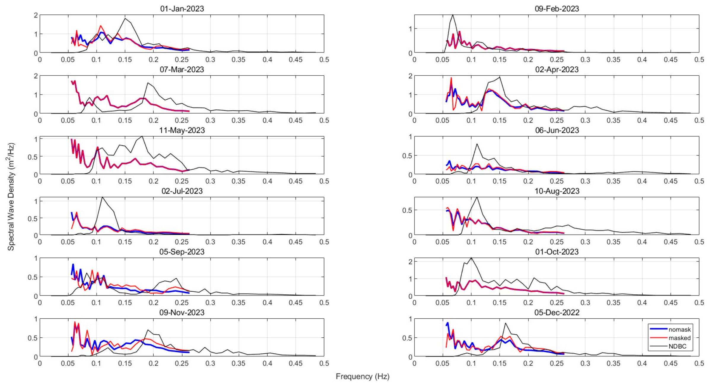
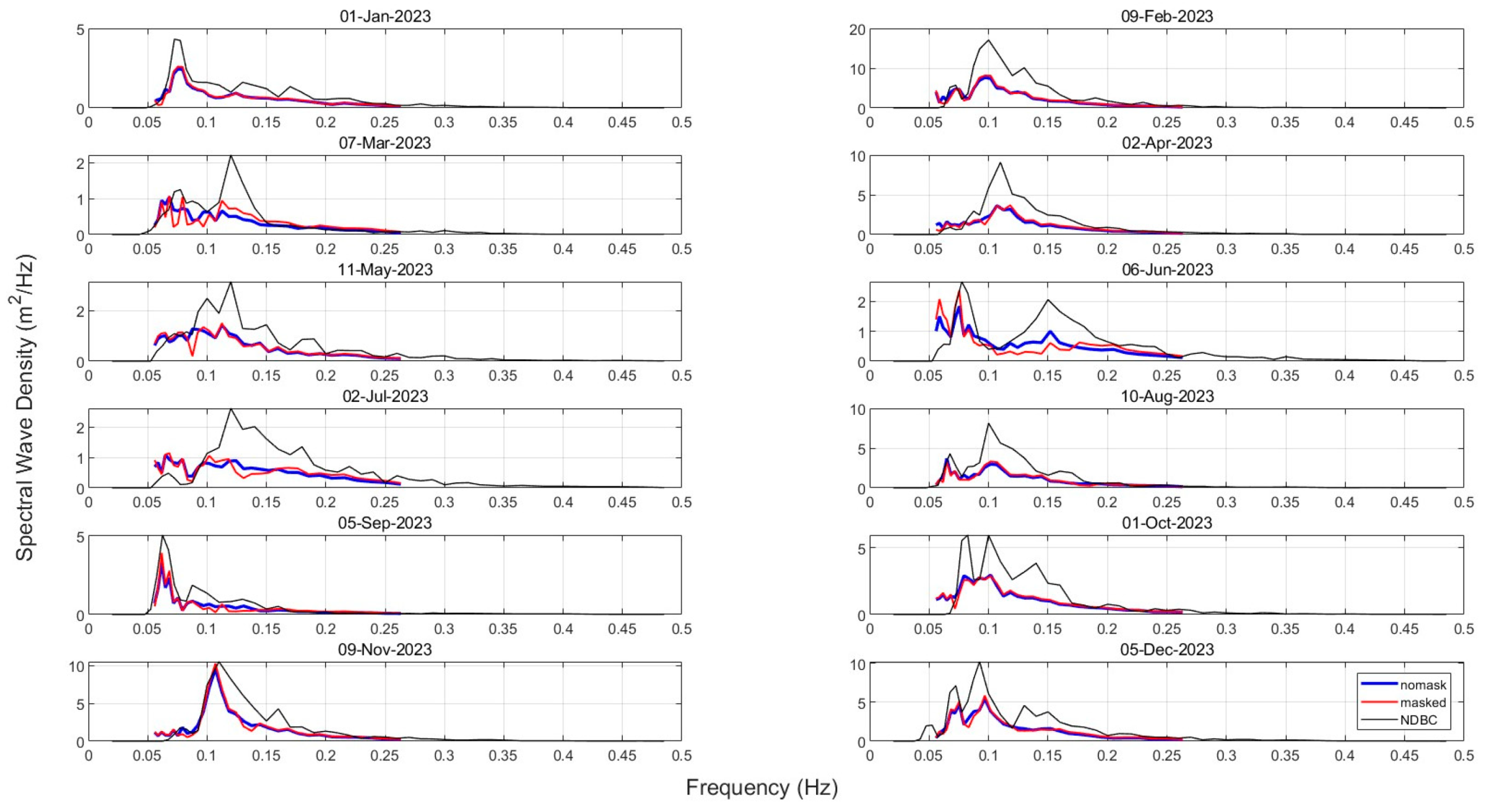
Since the operation period of CFOSAT is 13 days, after interpolating the CFOSAT orbits, two measurement buoys deployed in shallow and deep water were selected to match data for each of the 12 months, resulting in 12 sets of NDBC spectral data. In the nearshore region, due to spectral overlap between noise and valid signals, the observed wave spectrum shape and filtering effectiveness are relatively poorer (Figure 1). In contrast, CFOSAT exhibits stronger observational capability in deep water; parasitic peaks are easily identifiable, and the mask filtering method significantly suppresses low-frequency parasitic peaks (Figure 2). These results reflect the effectiveness of mask filtering for simple wave systems in deep water but highlight its limitations in complex nearshore environments.

2.7. Energy Calibration

After spectral conversion, energy calibration is necessary to balance the impact of mask filtering on total energy. According to Li et al. [45], the unmasked 10° beam data (${\mathrm{S}}_{{\mathrm{b}\mathrm{e}\mathrm{a}\mathrm{m}}_{10}}$) provides optimal energy, while the masked data (${\mathrm{S}}_{{\mathrm{b}\mathrm{e}\mathrm{a}\mathrm{m}}_{{10}_{\mathrm{m}}}}$) retains a finer spectral structure. The calibrated spectrum ${\mathrm{S}}_{\mathrm{n}\mathrm{e}\mathrm{w}}\left(\mathrm{f}\right)$ is obtained by:

$${\mathrm{S}}_{\mathrm{n}\mathrm{e}\mathrm{w}}\left(\mathrm{f}\right)={\mathrm{S}}_{{\mathrm{b}\mathrm{e}\mathrm{a}\mathrm{m}}_{{10}_{\mathrm{m}}}}\left(\mathrm{f}\right)\cdot {\displaystyle \frac{\int {\mathrm{S}}_{{\mathrm{b}\mathrm{e}\mathrm{a}\mathrm{m}}_{10}}\left(\mathrm{f}\right)\mathrm{d}\mathrm{f}}{\int {\mathrm{S}}_{{\mathrm{b}\mathrm{e}\mathrm{a}\mathrm{m}}_{{10}_{\mathrm{m}}}}\left(\mathrm{f}\right)\mathrm{d}\mathrm{f}}},$$

(11)

This ensures the total energy matches ${\mathrm{S}}_{{\mathrm{b}\mathrm{e}\mathrm{a}\mathrm{m}}_{10}}$ while preserving the spectral resolution of ${\mathrm{S}}_{{\mathrm{b}\mathrm{e}\mathrm{a}\mathrm{m}}_{{10}_{\mathrm{m}}}}$ [45].

Wind waves may be misclassified as swells due to the presence of low-frequency parasitic peaks. We validate the filtering rationality using the distribution of swells and wind sea. When the wave age β > 1.2, it is classified as a swell; when β < 0.8, it is classified as a wind sea; and when 0.8 < β < 1.2, it is considered a transitional state between wind sea and swell. Wave age β is calculated as:

$$\mathsf{\beta }={\displaystyle \frac{\mathrm{g}}{2\mathsf{\pi }{\mathrm{f}}_{\mathrm{p}}{\mathrm{U}}_{10}}},$$

(12)

where ${\mathrm{f}}_{\mathrm{p}}$ is the spectral peak frequency.

After introducing the wind-speed-dependent partition criterion and applying low-frequency filtering, the wave age calculated from the filtered and unfiltered CFOSAT wave spectrum was compared to the ERA5 wave age. The results showed that the proportion of wind waves with a wave age below 1.2 before filtration was 36%, while after filtration, it was 28% in January 2023, which is closer to the ERA5 results (

Table 2. The difference in wave age before and after filtering compared to ERA5 in January 2023.

	$\mathsf{\beta }$ < 1.2	$\mathsf{\beta }$ ≥ 1.2
Before filtering	36%	54%
After filtering	28%	72%
ERA5	19.8%	80.2%

).

2.8. High-Frequency Tail Spectrum Supplementation

Due to the limited observation of high-frequency waves (k > 0.2789 rad/m) by the satellite sensor, it is necessary to utilize the consistent power-law behavior of the omnidirectional wavenumber spectrum for high-frequency supplementation within the equilibrium and saturation ranges. The fixed slope of this spectral tail is typically represented as k⁻³, where k is the wavenumber. It describes the wave spectrum shape above the cutoff frequency and can be used to supplement the missing high-frequency part of the wave spectrum in CFOSAT data. This expression typically takes the following form:

$$\mathrm{F}\left(\mathrm{k}\right)=\{\begin{array}{c}{\mathrm{C}}_1{\mathrm{k}}^{-5/2}, {\mathrm{k}}_{\mathrm{c}}<k<{\mathrm{k}}_{\mathrm{n}}\\ {\mathrm{C}}_2{\mathrm{k}}^{-3}, {\mathrm{k}}_{\mathrm{n}}<k<{\mathrm{k}}_{\mathrm{m}}\end{array},$$

(13)

where $C_1=F\left(k_c\right)\cdot k_c^{5/2}$ and $C_2=C_1\cdot k_n^{1/2}$ are the coefficients calculated from the omnidirectional wavenumber spectrum at the observed cutoff wavenumber k_c and transition wavenumber k_n.

Referring to Phillips [29], the transition wavenumber k_n between the equilibrium range and the saturation range is defined as:

$${\mathrm{k}}_{\mathrm{n}}=\mathrm{g}\mathrm{r}/{\mathrm{u}}_{\ast }^2,$$

(14)

where r = 9.7 × 10⁻³.

The maximum frequency of the high-frequency tail is defined as the cutoff wavenumber k_m, above which the directional wave spectrum is assumed to be isotropic. The cutoff wavenumber follows Lenain and Melville [28]:

$$k_m=\left(\mathrm{g}/{\mathrm{u}}_{\ast }^2\right)\mathrm{e}\mathrm{x}\mathrm{p}\left[\left(\mathsf{\pi }/2-{\mathsf{\theta }}_0\right)/\mathsf{\gamma }\right],$$

(15)

where ${\mathsf{\theta }}_0$ = 2.835, $\mathsf{\gamma }$ = 0.48, and ${\mathrm{u}}^{\ast }=\sqrt{{\mathrm{C}}_{\mathrm{d}}}$ × ${\mathrm{U}}_{10}$ is the friction velocity. The drag coefficient ${\mathrm{C}}_{\mathrm{d}}$ is calculated using the piecewise function from Large and Pond [50] (1981):

$$\{\begin{array}{c}{\mathrm{C}}_{\mathrm{d}}=0.0012, \left|{\mathrm{U}}_{10}\right|\le 11 \mathrm{m}/\mathrm{s}\\ {\mathrm{C}}_{\mathrm{d}}=0.00049+0.000065\times \left|{\mathrm{U}}_{10}\right|, 11 \mathrm{m}/\mathrm{s}<\left|{\mathrm{U}}_{10}\right|\le 19 \mathrm{m}/\mathrm{s}\\ {\mathrm{C}}_{\mathrm{d}}=0.001364+2.34\times {10}^{-5}\times \left|{\mathrm{U}}_{10}\right|-2.3\times {10}^{-7}\times {\left|{\mathrm{U}}_{10}\right|}^2 19 \mathrm{m}/\mathrm{s}<\left|{\mathrm{U}}_{10}\right|\le 100 \mathrm{m}/\mathrm{s}\end{array},$$

(16)

To ensure the comparability between satellite observations, ERA5 reanalysis data, and on-site buoy data, this study established strict spatiotemporal matching criteria. Temporally, based on the observation time of the buoys, CFOSAT transit data within a matching time difference of ±30 min were selected, and ERA5 reanalysis data at the same time were extracted. Spatially, for CFOSAT’s irregular observation points, the nearest neighbor matching method was adopted, retaining only the closest observation points with a distance of no more than 50 km from the buoys; for ERA5’s regular grid, the nearest grid point method was used, retaining only matching data where the distance between the grid center and the buoy was no more than 0.2° (approximately 22 km). Matching points exceeding the above spatial threshold were eliminated to ensure that all analyses were conducted within an effective spatial scale.

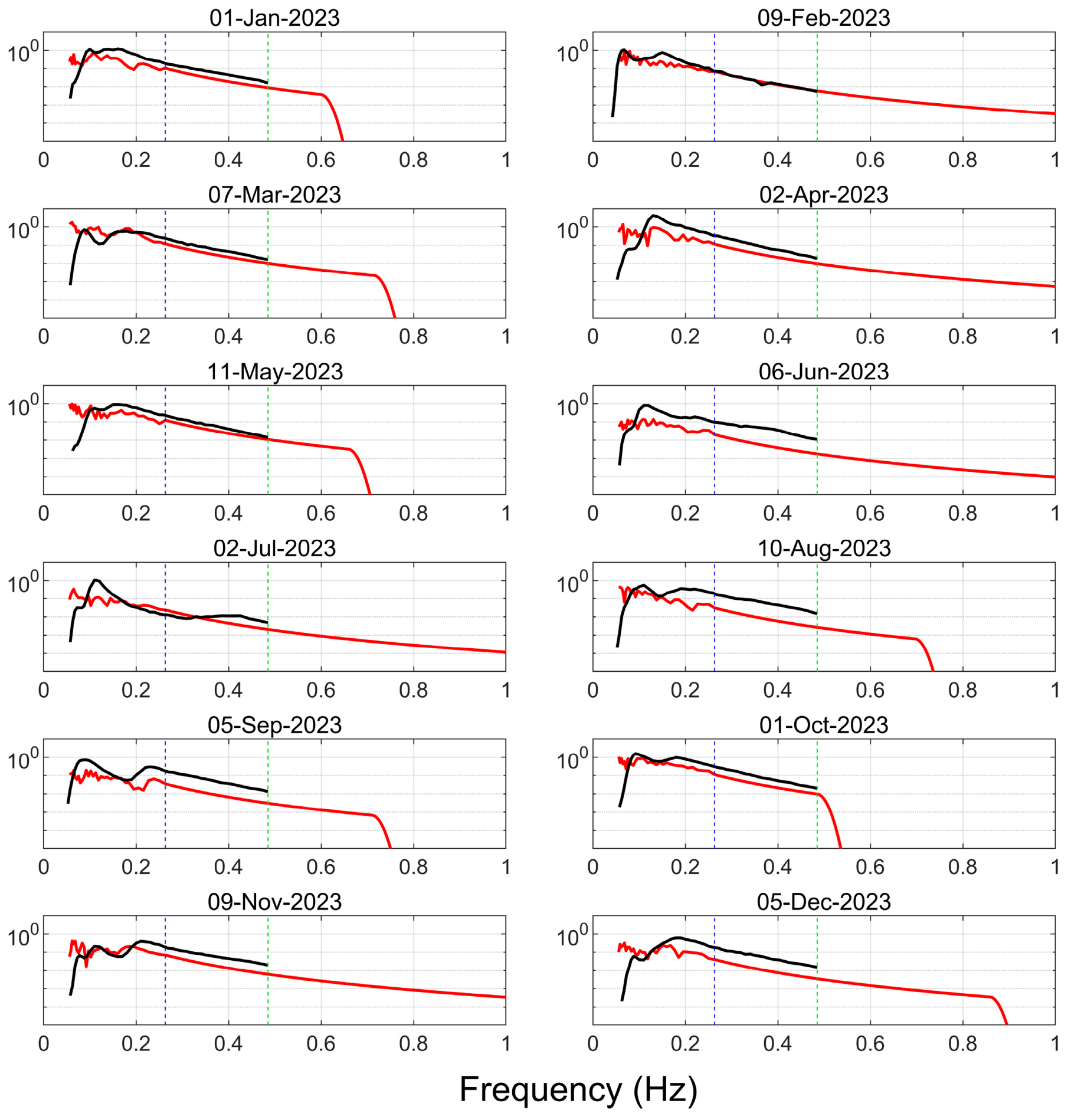
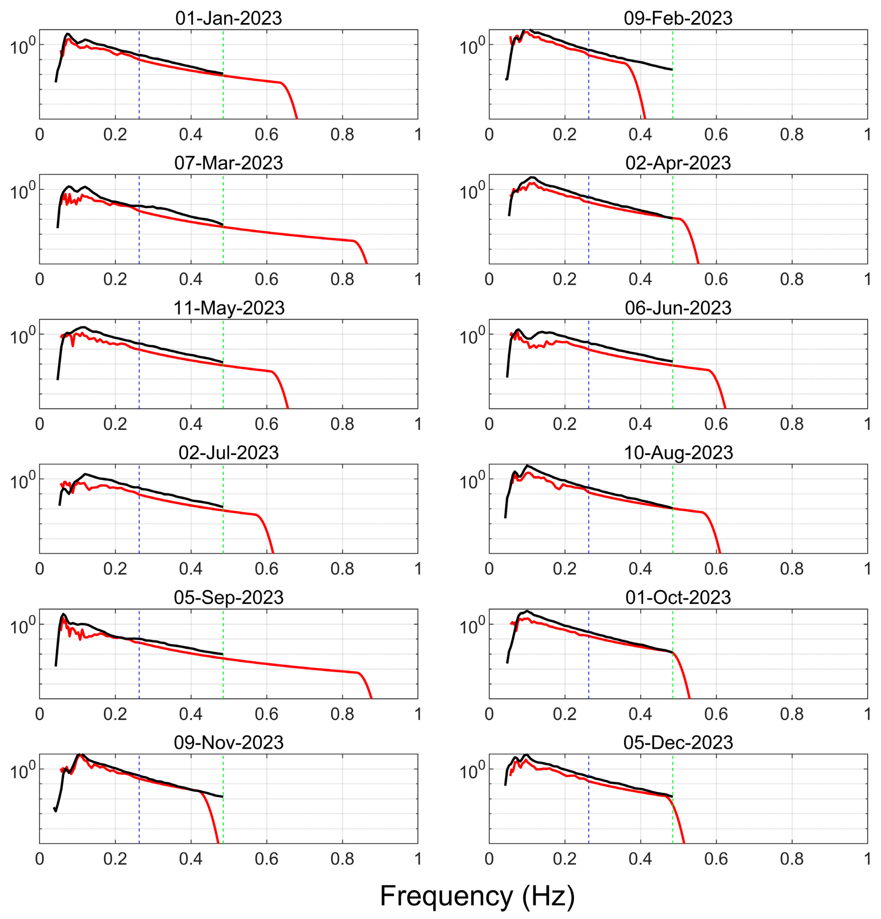
Figure 3 compares the measured wave spectrum at Buoy 41013 (33.441N, 77.764W) in shallow water with the CFOSAT wave spectrum before and after high-frequency supplementation. Figure 4 shows the same comparison at Buoy 51004 (17.538N, 152.23W) in deep water. From Figure 3, it can be seen that the spectral shape after high-frequency supplementation (red solid line) is consistent with the trend observed by the buoy (black solid line) in the range of 0.263–0.485 Hz, with an increase in energy. However, the supplemented spectrum is still slightly lower than that observed by the buoy. This may be due to the significant influence of seabed topography on shallow-water spectra, strong wave breaking and dissipation, and seabed friction causing the saturation zone spectrum to deviate slightly from the deep-water theoretical model, resulting in a slight deviation in the supplementation effect. From Figure 4, it can be seen that the frequency spectrum after high-frequency supplementation in the deep-water area matches well with the buoy observation results throughout the entire high-frequency range, and the energy trend is consistent. This indicates that the supplementary model based on Phillips’ saturation range theory has higher reliability in deep-water environments.

2.9. Stokes Drift Calculation

Stokes drift is calculated from the directional spectrum $\mathrm{F}\left(\mathrm{k}\right)$ according to [25]:

$${\mathrm{U}}_{\mathrm{s}}\left(\mathrm{z}\right)=2\iint \mathrm{F}\left(\mathrm{k}\right)\cdot \left[\mathsf{\omega }\left(\mathrm{k}\right)\cdot {\displaystyle \frac{\mathrm{c}\mathrm{o}\mathrm{s}\mathrm{h}\left[2\mathrm{k}\left(\mathrm{z}+\mathrm{h}\right)\right]}{2{\mathrm{s}\mathrm{i}\mathrm{n}\mathrm{h}}^2\left(\mathrm{k}\mathrm{h}\right)}}\right]\mathrm{d}\mathrm{k},$$

(17)

where k = |$\mathrm{k}$|, $\mathsf{\omega }\left(\mathrm{k}\right)=\sqrt{\mathrm{g}\mathrm{k} \mathrm{t}\mathrm{a}\mathrm{n}\mathrm{h}\left(\mathrm{k}\mathrm{h}\right)}$, and h is the water depth. The Stokes drift magnitude ${\mathrm{U}}_{\mathrm{s}}$(z) based on the omnidirectional wave spectrum $\mathrm{F}\left(\mathrm{k}\right)$ can be estimated as:

$${\mathrm{U}}_{\mathrm{s}}\left(\mathrm{z}\right)=2{\int }_{{\mathrm{k}}_{\mathrm{p}}}^{\mathrm{\infty }}\mathrm{F}\left(\mathrm{k}\right)\left[\mathsf{\omega }\left(\mathrm{k}\right)\cdot {\displaystyle \frac{\mathrm{c}\mathrm{o}\mathrm{s}\mathrm{h}\left[2\mathrm{k}\left(\mathrm{z}+\mathrm{h}\right)\right]}{2{\mathrm{s}\mathrm{i}\mathrm{n}\mathrm{h}}^2\left(\mathrm{k}\mathrm{h}\right)}}\right]\mathrm{k}\mathrm{d}\mathrm{k}.$$

(18)

Under deep-water conditions, since $\underset{\mathrm{k}\mathrm{h}\to \mathrm{\infty }}{\mathrm{l}\mathrm{i}\mathrm{m}}{\displaystyle \frac{\mathrm{c}\mathrm{o}\mathrm{s}\mathrm{h}\left[2\mathrm{k}\left(\mathrm{z}+\mathrm{h}\right)\right]}{2{\mathrm{s}\mathrm{i}\mathrm{n}\mathrm{h}}^2\left(\mathrm{k}\mathrm{h}\right)}}\approx {\mathrm{e}}^{2\mathrm{k}\mathrm{z}}, \mathsf{\omega }\approx \sqrt{\mathrm{g}\mathrm{k}}$, the above equation simplifies to:

$${\mathrm{U}}_{\mathrm{s}}\left(\mathrm{z}\right)=2{\int }_{{\mathrm{k}}_{\mathrm{p}}}^{\mathrm{\infty }}\mathrm{F}\left(\mathrm{k}\right)\sqrt{\mathrm{g}\mathrm{k}}{\mathrm{e}}^{2\mathrm{k}\mathrm{z}}\mathrm{k}\mathrm{d}\mathrm{k},$$

(19)

where ${\mathrm{k}}_{\mathrm{p}}$ is the spectral peak wavenumber of the wave spectrum, z is the depth, and $\mathrm{F}\left(\mathrm{k}\right)$ is the omnidirectional wave spectrum. The low-frequency drift ${\mathrm{U}}_{\mathrm{s}}^{\mathrm{l}\mathrm{o}\mathrm{w}}$ is obtained by integrating the spectrum from the peak wavenumber ${\mathrm{k}}_{\mathrm{p}}$ to the satellite observation cutoff wavenumber ${\mathrm{k}}_{\mathrm{c}}$: ${\mathrm{U}}_{\mathrm{s}}^{\mathrm{l}\mathrm{o}\mathrm{w}}\left(\mathrm{z}\right)=2{\int }_{{\mathrm{k}}_{\mathrm{p}}}^{{\mathrm{k}}_{\mathrm{c}}}\mathrm{F}\left(\mathrm{k}\right)\sqrt{\mathrm{g}\mathrm{k}}{\mathrm{e}}^{2\mathrm{k}\mathrm{z}}\mathrm{k}\mathrm{d}\mathrm{k}$. To quantify the contribution of high-frequency waves to Stokes drift, high-frequency contribution is defined as the proportion of high-frequency Stokes drift to the total drift volume:

$$\mathrm{c}\mathrm{o}\mathrm{n}\mathrm{t}\mathrm{r}\mathrm{i}\mathrm{b}\mathrm{u}\mathrm{t}\mathrm{i}\mathrm{o}\mathrm{n}=100\times {\displaystyle \frac{\left|{\mathrm{U}}_{\mathrm{s}}\left(z\right)-{\mathrm{U}}_{\mathrm{s}}^{\mathrm{l}\mathrm{o}\mathrm{w}}\left(z\right)\right|}{{\mathrm{U}}_{\mathrm{s}}\left(z\right)}},$$

(20)

Therefore, the spectral shape of surface waves directly influences Stokes drift. Note that because low-frequency waves are not steep, we neglect the contribution of very low wavenumbers to Stokes drift. As shown in

Table 3. Contribution of low-frequency part of wave spectrum to surface Stokes drift.

Season	Spring	Summer	Autumn	Winter
global seasonal mean Stokes (m/s) considering low freq	0.0412	0.0393	0.0408	0.0415
global seasonal mean Stokes (m/s) ignoring low freq	0.0404	0.0386	0.0401	0.0408
low-freq contribution (%)	1.8608	1.6978	1.7143	1.7671

, low freq represents low frequency waves, and their contribution to the total drift is very small, averaging only about 1.7%.

The transport of water particles caused by Stokes drift is termed Stokes transport, playing an important role in mass and energy exchange in the upper ocean. Stokes drift is vertically integrated over the depth to compute Stokes transport as below:

$${\mathrm{T}}_{\mathrm{s}}={\int }_{-{\mathrm{d}}_{\mathrm{s}}}^0{\mathrm{U}}_{\mathrm{s}}\left(\mathrm{z}\right)\mathrm{d}\mathrm{z},$$

(21)

where ${\mathrm{T}}_{\mathrm{s}}$ and ${\mathrm{U}}_{\mathrm{s}}\left(\mathrm{z}\right)$ are Stokes transport and Stokes drift, respectively; ${\mathrm{d}}_{\mathrm{s}}$ is the Stokes influence depth, defined as the maximum depth at which Stokes drift has not a significant vertical influence. If the water depth exceeds this depth, Stokes drift and its effects are negligible. ${\mathrm{d}}_{\mathrm{s}}$ can be calculated by ${\mathrm{d}}_{\mathrm{s}}={\displaystyle \frac{1}{2\mathrm{k}}}$, where $\mathrm{k}$ is the wavenumber, $\mathrm{k}={\displaystyle \frac{2\mathsf{\pi }}{\mathsf{\lambda }}}$, and $\mathsf{\lambda }$ is the wavelength.

3. Results

3.1. Filtering

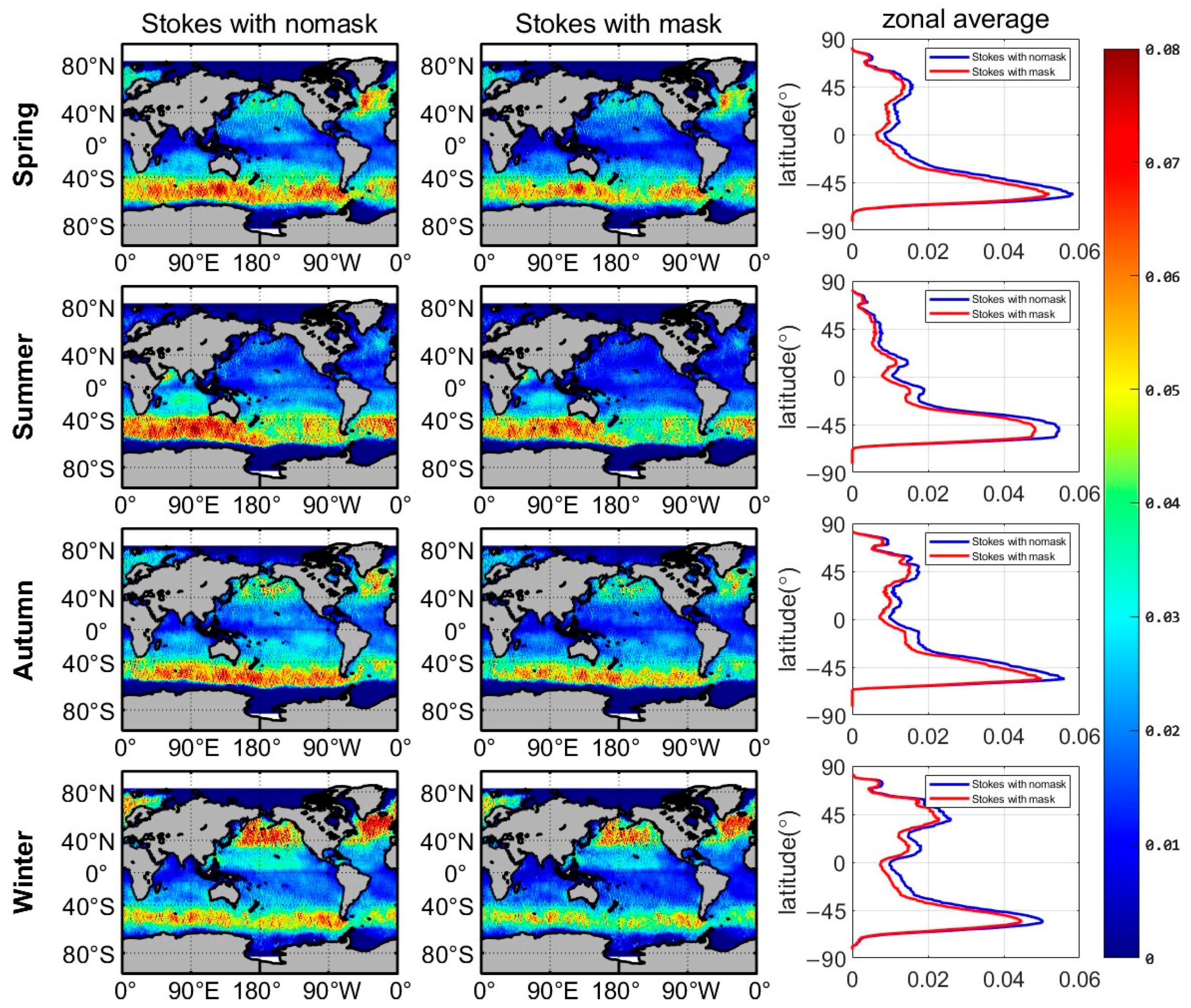
To evaluate the impact of filtering on Stokes drift estimation, we compared the global sea-surface Stokes drift calculated from CFOSAT wave spectra before and after mask filtering. The results show that the filtering process, while suppressing low-frequency parasitic peaks, exerts a systematic influence on the estimated Stokes drift.

As shown in Figure 5, the effect of filtering on Stokes drift is more pronounced in high-latitude wind-dominated regions, such as the Southern Ocean and the winter wind zones of the North Pacific. Before filtering, the average sea-surface Stokes drift in the circumpolar Southern Ocean region based on the original SWIM spectra reached up to 0.06 m/s, whereas after filtering, this value decreased to 0.04 m/s. Although the filtering may attenuate some valid high-frequency information, it plays a positive role in suppressing low-frequency noise and improving the structural rationality of the wave spectrum, thereby enhancing the accuracy of Stokes drift calculations to a certain extent. This offers valuable insights for further improving the applicability of CFOSAT wave spectra under complex sea states.

3.2. Maximum Cutoff Frequency

Statistics of the k_m calculation results are presented in

Table 4. Seasonal proportion of wave spectra that are supplementable and require supplementation.

Season	Spring	Summer	Autumn	Winter
Supplementable	99.3238%	99.4679%	99.5274%	99.5098%
Requiring Supplementation	99.7740%	99.9185%	99.9915%	99.9254%

. For wave spectra observed by CFOSAT where the spectral peak k_p is less than the observed cutoff wavenumber k_c, meaning the spectral peaks of the wave spectra appear normally and maintain the basic complete spectral shape, we classify them as “supplementable” wave spectra, and these account for over 99% in all four seasons. The spectra where the observed maximum cutoff wavenumber k_c is less than the theoretical maximum cutoff wavenumber k_m are classified as “requiring supplementation” wave spectra, and these also account for over 99% in all seasons. Therefore, supplementing the high-frequency part of CFOSAT-observed wave spectra is necessary.

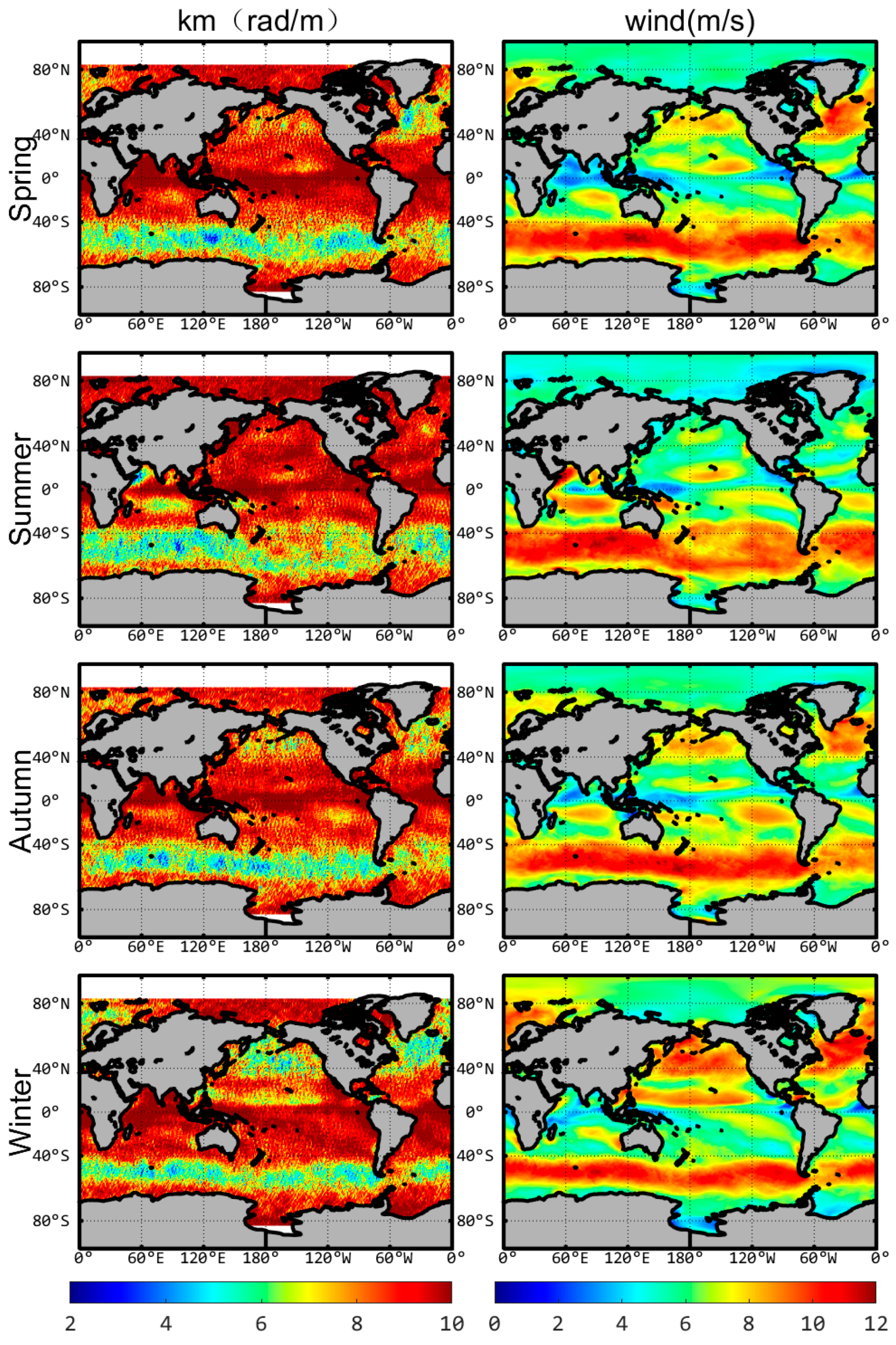
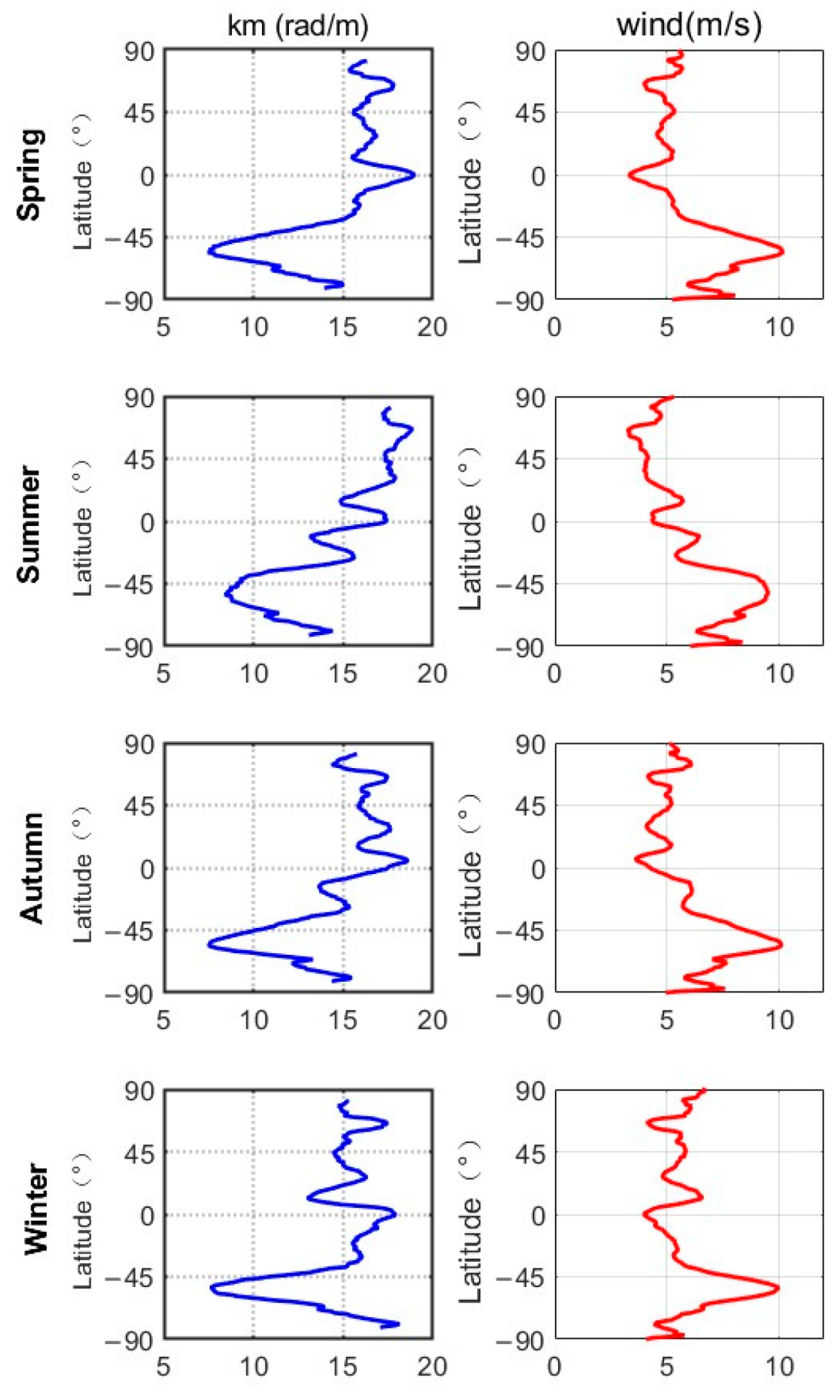
Comparing the seasonal distribution of k_m with sea surface wind speed (Figure 6 and Figure 7), k_m exhibits distinct spatial characteristics. In equatorial low-wind regions (average wind speed as low as 1 m/s), k_m peaks can reach 10 rad/m or higher. In contrast, in the Southern Ocean high-wind band (average wind speed exceeding 10 m/s), k_m shows a pronounced low-value zone, dropping to as low as 1 rad/m. A distinct low-value zone of k_m appears in the North Pacific in winter and in the Indian Ocean in summer. This is because a significant high-wind zone appears in the mid–high latitudes of the North Pacific in winter (average wind speed 10–15 m/s), while large-scale low-wind zones (average wind speed often below 4–6 m/s) occur in the tropical North Indian Ocean (especially the northern Arabian Sea, Bay of Bengal, and equatorial Indian Ocean) in summer. This inverse correlation between k_m and wind speed is consistent with Phillips [29], where strong winds enhance breaking dissipation, maintaining the saturated shape of the high-frequency spectrum and suppressing its excessive development.

3.3. Comparison with Buoys

Due to the operational period of CFOSAT being 13 days, after interpolating the satellite tracks, this study selected 240 matched datasets (10 buoys × 24 time phases) based on 10 measured buoy locations, obtaining 240 NDBC-measured wave spectra, and the sea surface Stokes drift was calculated from these measured wave spectra. Please note that since the theoretical maximum cutoff frequency after supplementation is usually higher, when compared with buoy data, the cutoff frequency of the supplemented CFOSAT spectrum must be set to be the same as the buoy’s cutoff frequency, which is 0.485 Hz (0.945 rad/m).

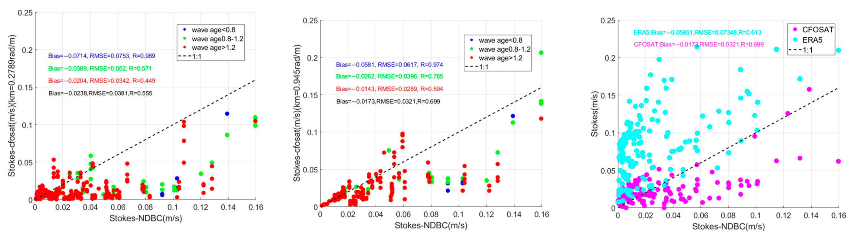
To evaluate the effectiveness of high-frequency supplementation in the system, we divided the data into three groups based on wave age ($\mathsf{\beta }$): wind-wave-dominant ($\mathsf{\beta }$ < 0.8), transitional (0.8 ≤ $\mathsf{\beta }$ < 1.2), and swell-dominant ($\mathsf{\beta }$ ≥ 1.2), and we conducted comparative analysis for each group. Overall, high-frequency supplementation effectively improved estimation accuracy. Figure 8 and Figure 9 show that in the wind-wave-dominant region ($\mathsf{\beta }$ < 0.8), the bias improved from −0.0706 m/s to −0.0653 m/s, the root mean square deviation RMSD decreased from 0.0755 m/s to 0.0699 m/s, and the correlation coefficient R increased from 0.977 to 0.989, indicating that the high consistency between the spectral shape and the actual situation is maintained under wind and sea conditions. In the transition zone (0.8 ≤ $\mathsf{\beta }$ < 1.2), RMSD significantly reduced from 0.0493 m/s to 0.0423 m/s and the correlation coefficient R significantly increased from 0.602 to 0.788, indicating good adaptability of the supplementary method to mixed sea conditions. In the region dominated by swells ($\mathsf{\beta }$ ≥ 1.2), bias decreased from −0.0187 m/s to −0.0179 m/s, RMSD decreased from 0.0326 m/s to 0.0303 m/s, and the correlation coefficient R increased from 0.466 to 0.627.

To further verify the reliability of this method, the CFOSAT Stokes drift after high-frequency supplementation and the Stokes drift from ERA5 reanalysis data were each compared with buoy observations. Figure 10 shows that the RMSD between the CFOSAT-supplemented results and the buoy was 0.0321 m/s, with a correlation coefficient of 0.699; the RMSD between ERA5 and the buoy is 0.07348 m/s, with a correlation coefficient of 0.613. Obviously, the Stokes drift obtained by the method in this article is superior to the widely used ERA5 reanalysis data in terms of bias and correlation. This indicates that based on CFOSAT spectroscopy and supplemented by the high-frequency supplement scheme proposed in this study, a more reliable and accurate global sea surface Stokes drift product can be obtained, which can be used for the analysis of its large-scale spatiotemporal evolution characteristics.

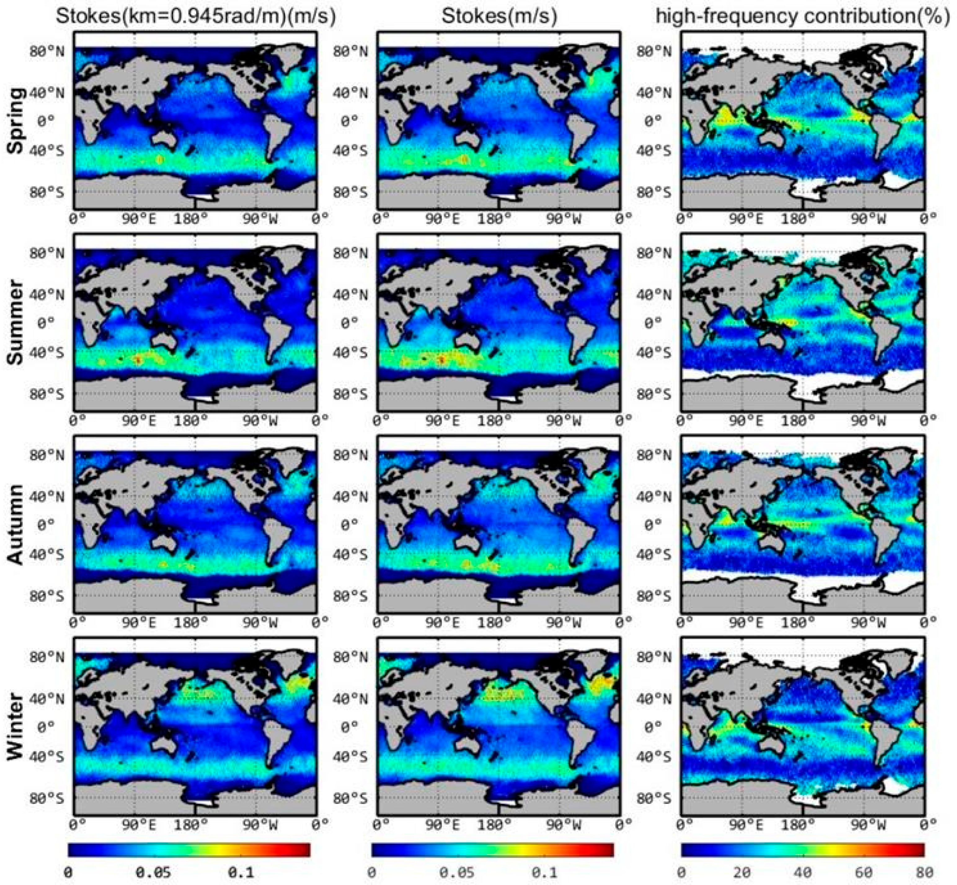
Figure 9 and

Table 5. Stokes drift magnitude at different cutoff frequencies. Herein, Max denotes the maximum value, and Ave denotes the average value.

Season	Spring (Max)	Summer (Max)	Autumn (Max)	Winter (Max)	Spring (Avg)	Summer (Avg)	Autumn (Avg)	Winter (Avg)
Surface Stokes (m/s) at cutoff freq 0.485 Hz	1.5216	1.9023	2.7163	3.2853	0.0406	0.0383	0.0403	0.0413
Surface Stokes (m/s) at max cutoff freq	3.2	4.6578	5.9250	7.8619	0.0493	0.0462	0.0492	0.0499
HF contribution (%)	52.45	59.1588	54.1553	58.2139	17.6741	17.0996	18.0894	17.2345

further confirm the contribution of high frequencies to Stokes drift, and HF in Table 5 represents high frequency. Setting the wave spectrum cutoff frequency to 0.485 Hz and with the theoretical maximum cutoff frequency, the average high-frequency contributions above 0.485 Hz across the four seasons were 17.7%, 17.1%, 18.1%, and 17.2% of the total Stokes drift, respectively, with maxima reaching 58%. This aligns with the conclusion of Lenain and Pizzo [25] that “neglecting high frequencies underestimates Us by over 50%.” Since the contribution of high frequencies is obvious, we proceed to discuss its impact on Stokes drift.

3.4. Comparison with ERA5

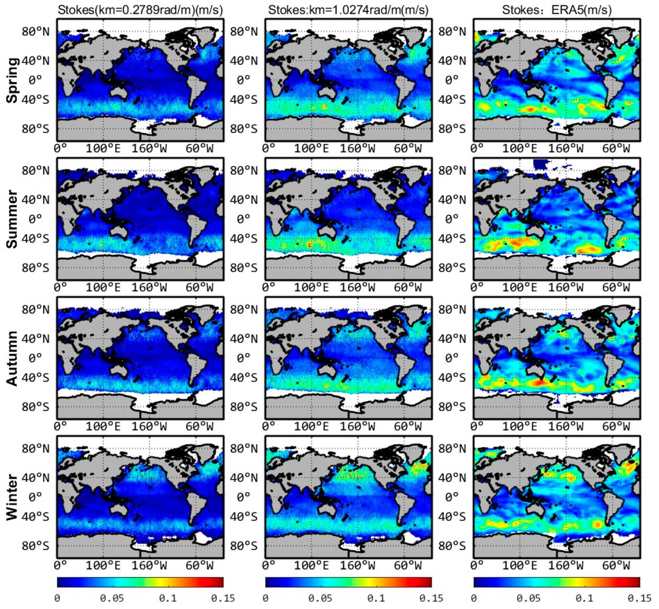
Figure 10 shows the distribution characteristics of the seasonal average sea surface Stokes drift velocity calculated using different wave spectra. Note that when comparing with ERA5 data, the cutoff frequency of the supplemented CFOSAT wave spectrum must be set to match ERA5’s cutoff frequency of 0.5478 Hz (1.2074 rad/m) because the theoretical maximum cutoff frequency is higher. We found that different datasets exhibit consistent spatial distribution characteristics. The maximum sea surface Stokes drift velocity occurs in the Antarctic Circumpolar Current region in all seasons, with a smaller peak around 60°N. Except for winter, all seasons show a significant distribution pattern of being stronger in the south and weaker in the north. As shown in

Table 6. Comparison of average Stokes drift before/after HF supplementation and ERA5.

Season	Spring (m/s)	Summer (m/s)	Autumn (m/s)	Winter (m/s)
CFOSAT Stokes pre-HF supp	0.0299	0.0281	0.0292	0.0301
CFOSAT Stokes post-HF supp	0.0471	0.0442	0.0323	0.0478
ERA5 Stokes (m/s)	0.0433	0.0413	0.04223	0.0442

, where pre-HF supp in Table 6 represents before high-frequency supplementation and post-HF supp represents after high-frequency supplementation, supplementing the high-frequency part of the wave spectrum reduces the bias between CFOSAT and ERA5 data. Before supplementation, although Stokes drift showed significant peaks in the Antarctic Circumpolar Current region, other areas showed little variation, with seasonal Stokes drift averages around 0.03 m/s. After supplementation, Stokes drift showed clear differences in the Northern Hemisphere, particularly in the North Pacific and North Atlantic regions across seasons, with seasonal averages around 0.04 m/s. The absolute bias between CFOSAT and ERA5 decreased from 0.0134 m/s (spring), 0.0132 m/s (summer), 0.01303 m/s (autumn), and 0.0141 m/s (winter) before supplementation to 0.0038 m/s (spring), 0.0029 m/s (summer), 0.00323 m/s (autumn), and 0.0036 m/s (winter) after supplementation. As shown in

Table 7. Bias (%) of Stokes drift relative to ERA5 before/after HF supplementation.

Season	Spring	Summer	Autumn	Winter
Bias pre-supp (%)	31.0769	31.9613	30.7814	31.9759
Bias post-supp (%)	8.7760	7.0218	7.66	8.1448

, where Bias pre-supp in Table 7 represents the bias before high-frequency supplementation and Bias post-supp represents the bias after high-frequency supplementation, the relative bias between Stokes drift calculated before and after supplementation and ERA5 data decreased from 31.08%, 31.96%, 30.78%, and 31.98% to 8.78%, 7.02%, 7.66%, and 8.14% respectively, improving accuracy by over 20%. Both absolute and relative deviations have been reduced, indicating that our proposed new method is reliable and can be used to analyze the spatiotemporal evolution characteristics of global Stokes drift.

3.5. Stokes Drift

3.5.1. High-Frequency Contribution Distribution

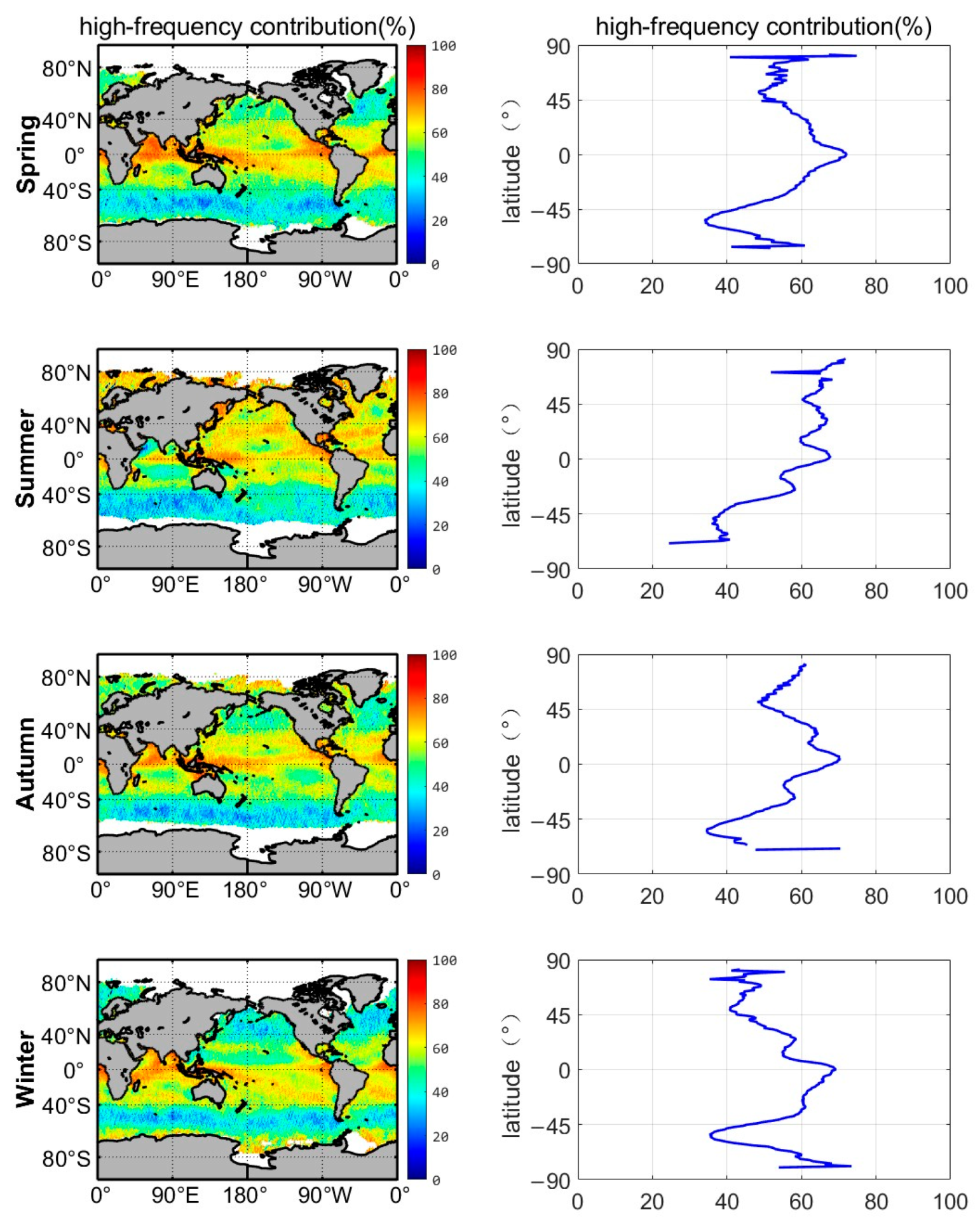
Emphasizing the contribution of high-frequency waves to surface Stokes drift is increasingly recognized as important. Lenain and Pizzo [25] pointed out that ignoring waves with frequencies above 0.5 Hz may lead to an underestimation of surface Stokes drift by more than 50%. Based on this, we describe specific spatial heterogeneity. We find that the high-frequency contribution is not uniformly large but is strongly modulated by the local wind speed. Using the theoretical maximum cutoff frequency k_m from Equation (15) to calculate Stokes drift, the high-frequency contribution was further derived. As shown in Figure 11, the high-frequency contribution exhibits significant zonal characteristics consistent with the k_m distribution in Figure 6. The minimum values occur in the high-wind band of the Southern Ocean (U₁₀ > 10 m/s) across all seasons. This is because strong winds enhance wave breaking dissipation [29], suppressing the development of the high-frequency spectrum. The high-frequency contribution reaches its maximum near the equator, averaging close to 80%, especially exceeding 80% in the Indian Ocean and eastern Pacific. As shown by Equation (15), the maximum cutoff frequency k_m is inversely proportional to wind speed. Therefore, the distribution of the wind field inevitably modulates the distribution of k_m, thereby influencing the distribution of the high-frequency contribution to the Stokes drift. This indicates that the variation characteristics of the high-frequency contribution to Stokes drift are closely linked to the global sea surface wind field. This wind-modulated zonal asymmetry, quantified globally here, was not previously captured in existing studies.

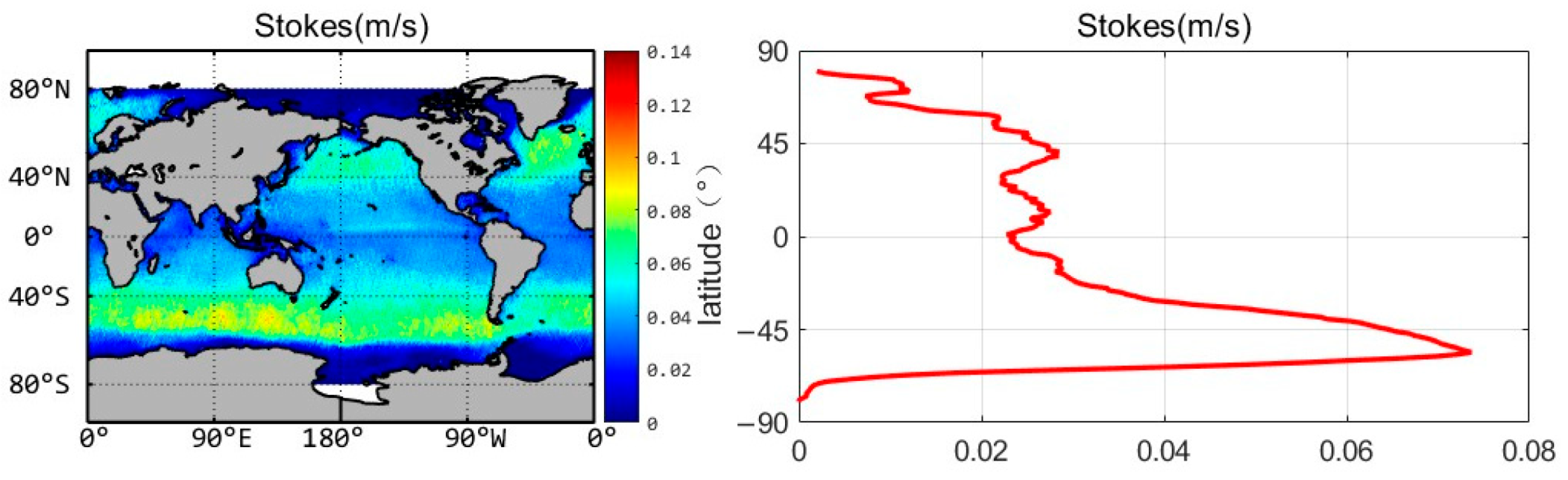
3.5.2. Sea Surface Stokes Drift Distribution

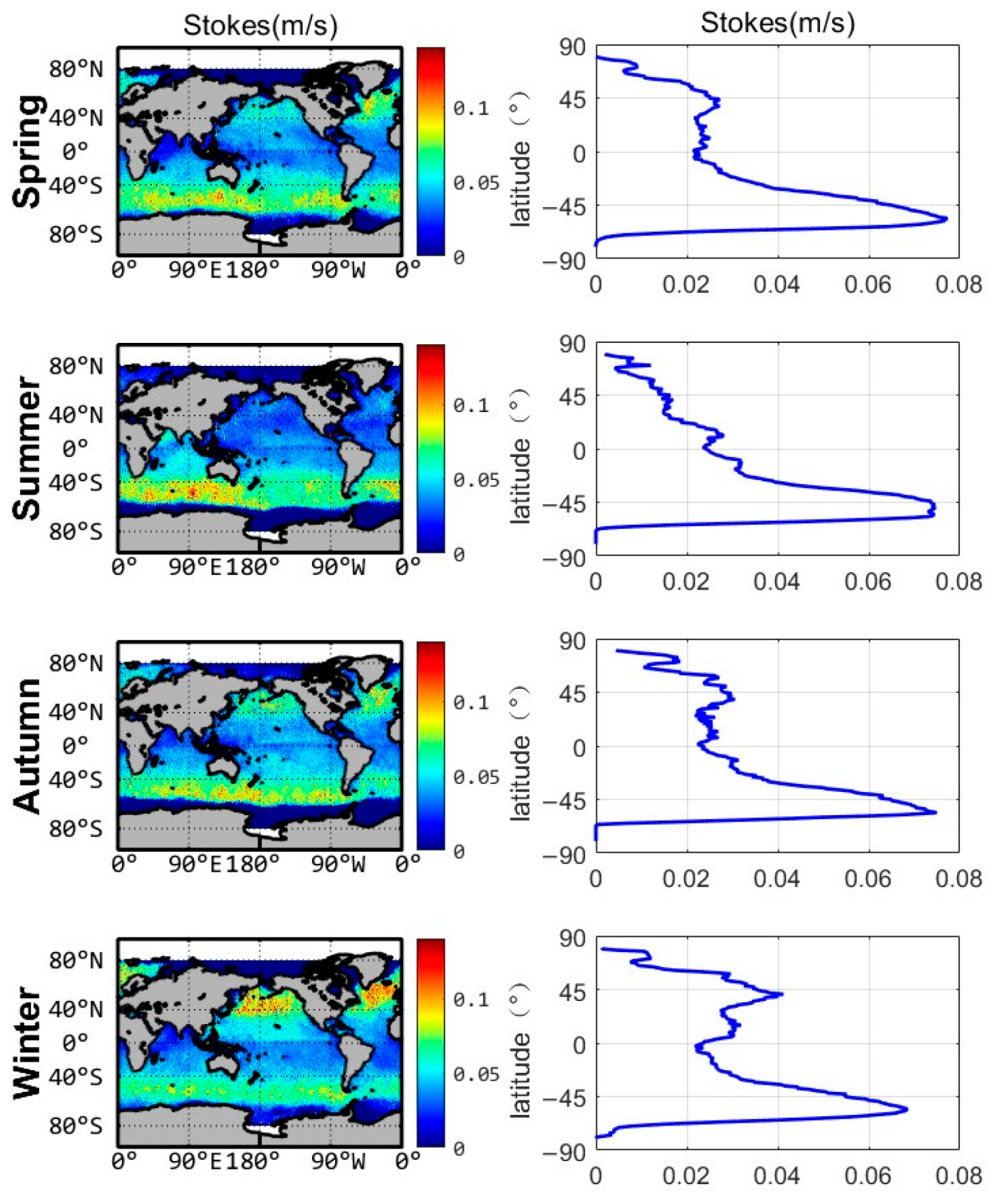
Figure 12 and Figure 13 show the distribution characteristics of the seasonal and annual average sea surface Stokes drift velocity, which is generally consistent with previous studies based on numerical models or scatterometer data [49,50]. Common features across all seasons are evident: a banded distribution of the maximum Stokes drift magnitude occurs across the vast Southern Ocean region between 40~60°S. The seasonal variation in the Southern Hemisphere is also quite significant, being weakest in winter (average Stokes drift is 0.05 m/s), gradually strengthening from spring, and reaching its maximum in summer (exceeding 0.12 m/s). This is related to the annual cycle of westerly wind intensity. In the Northern Hemisphere, modulated by storm track migration, the maximum Stokes drift is located in the eastern boundary regions of the North Pacific and North Atlantic. Its seasonal pattern is opposite to that of the Southern Hemisphere: maximum in winter (exceeding 0.12 m/s) and minimum in summer (mostly < 0.05 m/s in the North Atlantic with little variation). Furthermore, among the major oceans, the North Atlantic exhibits the most pronounced seasonal variation amplitude, followed by the North Pacific, and the Indian Ocean shows the smallest variation. The overall distribution shows a pattern of stronger in the south and weaker in the north annually. The maximum value occurs in the Antarctic Circumpolar Current, exceeding 0.12 m/s (average > 0.073 m/s). Smaller peaks reaching 0.08 m/s appear in the North Pacific and Northwest Atlantic. The minimum values occur near the equator and the poles.

3.5.3. Stokes Transport

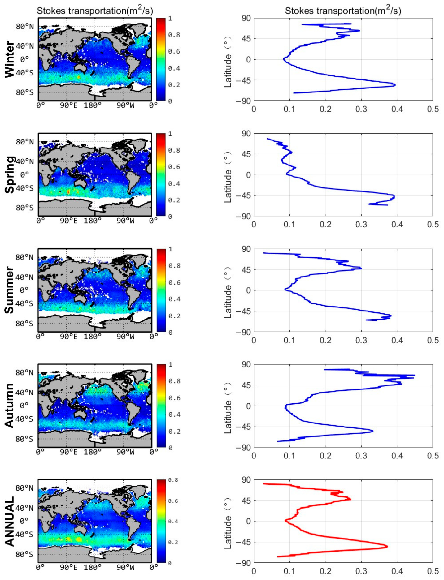
Using Equation (21) and the Stokes drift calculated by the supplemented wave spectrum, the global distribution of Stokes transport can be calculated and analyzed. Figure 14 shows the characteristics of the seasonal average global Stokes transport distribution. Overall, except in winter, the pattern shows larger values in the Southern Hemisphere than in the Northern Hemisphere and larger values in high-latitude seas than in low-latitude seas. In the Northern Hemisphere, Stokes transport reaches its maximum in the North Pacific and North Atlantic westerly wind regions in winter, exceeding 1 m²/s, and the latitudinal average can reach 0.5 m²/s, which is the largest Stokes transportation among the four seasons; it reaches its minimum in summer, dropping below 0.2 m²/s in the North Pacific, and the latitudinal average decreases to 0.14 m²/s. Conversely, Southern Ocean Stokes transport reaches its maximum in summer, exceeding 1 m²/s; it reaches its minimum in winter, around 0.5 m²/s.

Figure 14 shows the annual average Stokes transport distribution. The annual average Stokes transport largely shares the same overall characteristics as the seasonal averages: larger in the Southern Hemisphere than in the Northern Hemisphere, and larger in high-latitude seas than in low-latitude seas. In the Northern Hemisphere, the annual average maximum Stokes transport is located in the North Atlantic between 50°~60°N, exceeding 0.6 m²/s. In the high-latitude North Pacific, the maximum Stokes transport exceeds 0.5 m²/s. Over most of the Southern Ocean, the maximum Stokes transport reaches 0.7 m²/s, located around 50°S between 60°~120°E. In low-latitude regions near the equator, Stokes transport shows a banded distribution, with an average minimum below 0.12 m²/s.

4. Discussion

By comparing the high-frequency supplemented CFOSAT spectra with buoy and ERA5 reanalysis data from multiple angles, the estimation results of this study were validated and revealed a series of phenomena worth further exploration and their underlying physical mechanisms.

Firstly, although the high-frequency supplementation scheme has comprehensively improved the estimation accuracy of Stokes drift, its performance varies under different sea conditions, and the improvement is relatively limited in sea conditions dominated by swells. This is mainly due to two reasons: firstly, the energy of the swell is concentrated in the low frequency, and the contribution of the high-frequency part itself is relatively small. Therefore, even if the high-frequency tail spectrum is supplemented, the overall improvement in the total Stokes drift is limited; secondly, the current wind-speed-dependent parametric model is mainly based on the wind–sea relationship and does not fully consider the possible effects of long wave modulation or nonlinear wave–wave interactions on the high-frequency part under the background of surging waves. In addition, swells often occur outside the wind zone, and the development of their high-frequency saturation range may be constrained by more complex energy dissipation mechanisms. Therefore, there is still room for improvement in the ability of the current model to capture the fine structure of high-frequency spectra under the dominant sea conditions of surging waves. Future research can explore the introduction of parameters such as wave age and peak period of swell, establish a high-frequency tail spectrum model dependent on swell, or combine direction constraints provided by SAR inversion spectra to further improve the estimation accuracy of Stokes drift under mixed sea conditions. when wave age was not distinguished, overall, Bias decreased from −0.0238 m/s to −0.0173 m/s, RMSD decreased from 0.0381 m/s to 0.0321 m/s, and the correlation coefficient R increased from 0.555 to 0.699, proving the overall effectiveness of this scheme.

When comparing the products of this method with reanalysis data, we found that there are still some systematic differences between the estimated results based on CFOSAT SWIM spectra and ERA5 data. This difference is partly due to the different ways in which the two handle high-frequency wave spectra. Our parameterization scheme, by introducing a wind-speed-dependent cutoff wavenumber, better characterizes the breaking and dissipation suppression effect under high-wind conditions. This echoes the viewpoint of Sánchez-Arcilla et al. [33] that input field errors can be amplified in coastal forecasting: in the strong wind field of the Southern Ocean, even subtle differences in the shape of the high-frequency tail of the wave spectrum (such as the slope of the saturation region and the cutoff frequency) can be amplified through the Stokes drift calculation formula, leading to different final drift fields. Therefore, the method proposed in this paper not only provides an improved Stokes drift product, but more importantly, it provides a powerful tool for us to understand the physical mechanisms behind the differences between different wave data sources.

We further explored the modulation factors that affect the high-frequency contribution of Stokes drift. This study suggests that although sea surface wind speed modulates the Stokes high-frequency contribution, it is difficult to accurately fit all data points at a global scale using a simple univariate function, as high-frequency contributions may be significantly influenced by other ocean dynamic factors in addition to wind speed. We analyze that wave age may be a key common modulation factor. At the same wind speed, developing waves and fully developed waves have different spectral shapes, which affects the energy of the high-frequency part. In addition, the spatial variability in wave breaking dissipation, the degree of mixing between swell and wind waves, and the vertical shear of the upper ocean may introduce additional complexity. In the future, it is necessary to construct a multivariate empirical model to achieve high-precision parameterization of high-frequency contributions.

Compared with some studies based on numerical models or scatterometer inversion, our estimation based on CFOSAT SWIM spectra shows a lower performance. For instance, the model-based results of Zhang et al. [51] show extensive areas in the Southern Ocean with Stokes drift exceeding 0.1 m/s, while Liu et al. [52] report a global average of 0.09 m/s from scatterometer retrievals. In contrast, our estimates based on CFOSAT SWIM spectra yield a global annual mean of approximately 0.05 m/s. This systematic underestimation can be primarily attributed to the residual effects of high-frequency spectral truncation and the influence of a mixed sea state. Although a parameterization scheme was used to supplement the high-frequency tail, the Stokes drift was often calculated using a cutoff frequency matched to the validation data rather than the higher theoretical maximum, which conservatively limits the contribution from the very high frequencies that are most significant for the drift. Furthermore, the potential incomplete separation of wind seas and swells in complex sea states might result in the spectra retaining more low-frequency swell energy, which contributes less to the net drift, thereby lowering the overall averaged value compared to methods that more directly isolate the dominant wind sea component. At present, precise global quantification of this underestimation level faces fundamental challenges, as there is a lack of an independent, complete, and fully covered global dataset of measured values as a calibration benchmark, and there are complex nonlinear interactions between various error sources. Therefore, the core objective of this study is to propose an improved high-frequency supplementation method and evaluate its superiority over existing data sources such as ERA5, as well as to reveal the global distribution characteristics of Stokes drift and high-frequency contributions. We have demonstrated through detailed comparative analysis that our method outperforms ERA5 reanalysis data in terms of correlation, bias, and spatial consistency, providing a solid data foundation for understanding the macroscopic dynamic structure of global Stokes drift. In the future, more extensive high-frequency field observation data will be utilized to construct robust error models for accurate global quantification and correction of systematic underestimation. Consequently, this study provides a conservative yet physically based estimate of global Stokes drift derived directly from satellite wave spectra, highlighting the systematic underestimation inherent when relying on the current spectral observing capabilities and underscoring the critical importance of addressing the high-frequency truncation issue.

5. Conclusions

This study utilizes CFOSAT satellite observations, buoy validation, and ERA5 reanalysis data, reveals the critical impact of the high-frequency wave spectrum on Stokes drift calculation and analyzes its global distribution characteristics and dynamic mechanisms. The main results are as follows.

The absence of high-frequency wave spectra is the core source of bias in Stokes drift estimation from CFOSAT. While mask filtering based on SWIM directional spectra effectively suppresses low-frequency parasitic peaks, its limited wavenumber coverage (k_max = 0.2789 rad/m) causes high-frequency energy truncation. By introducing the wind-speed-modulated transition wavenumber k_n and high-frequency tail spectrum model, supplementing the high frequencies in CFOSAT data significantly improved Stokes drift accuracy. Compared with the buoy data, the results after high-frequency supplementation and before high-frequency supplementation were improved from R = 0.555 to R = 0.699. At the same time, comparing the high-frequency supplemented results and ERA5 reanalysis data with the buoy data, it was found that the accuracy of the results obtained by this method (R = 0.699) was superior to the widely used ERA5 reanalysis data (R = 0.613), which clarified the advantages of this method in obtaining reliable Stokes drift data.

Based on this reliable method, we have described the high-frequency contribution distribution characteristics of global Stokes drift. Our results indicate that the latitudinal differences in high-frequency contributions are controlled by sea surface wind speeds, exceeding 80% in low-wind equatorial regions (U₁₀ < 4 m/s), which validates Lenain and Pizzo’s [25] assertion that “ignoring high-frequency will underestimate Stokes drift by more than 50%.” Additionally, we found that in the Southern Ocean high-wind band (U₁₀ > 10 m/s), due to enhanced fragmentation dissipation suppressing the development of saturation range, high-frequency contributions will decrease to below 10%. Furthermore, we have revealed the temporal and spatial characteristics of global Stokes drift. The global surface Stokes drift field exhibits significant hemisphere asymmetry and seasonal evolution, with high values maintained throughout the Antarctic Circumpolar Current region and peak values observed in the Northern Hemisphere wind zone during winter.

Accurate characterization of the high-frequency contribution through this study can optimize predictions of drifting object trajectories (e.g., plastic transport), parameterization of Langmuir turbulence mixing, and air–sea flux estimation. It holds application value for improving the simulation of upper-ocean processes in climate models. Future research will optimize the separation and high-frequency supplementation methods of spectra under complex sea conditions and combine more on-site observation data to construct error models to correct system biases.

References

1. Stokes, G.G. (Ed.) Supplement to a memoir on some cases of fluid motion. In Mathematical and Physical Papers; Cambridge University Press: Cambridge, UK, 2009; pp. 188–196. [Google Scholar] [CrossRef]
2. Rascle, N.; Ardhuin, F.; Queffeulou, P.; Croizé-Fillon, D. A global wave parameter database for geophysical applications. Part 1: Wave-current–turbulence interaction parameters for the open ocean based on traditional parameterizations. Ocean Model. 2008, 25, 154–171. [Google Scholar] [CrossRef]
3. Breivik, Ø.; Janssen, P.A.E.M.; Bidlot, J.-R. Approximate Stokes drift profiles in deep water. J. Phys. Oceanogr. 2014, 44, 2433–2445. [Google Scholar] [CrossRef]
4. Webb, A.; Fox-Kemper, B. Wave spectral moments and Stokes drift estimation. Ocean Model. 2011, 40, 273–288. [Google Scholar] [CrossRef]
5. Dobler, D.; Huck, T.; Maes, C.; Grima, N.; Blanke, B.; Martinez, E.; Ardhuin, F. Large impact of Stokes drift on the fate of surface floating debris in the South Indian Basin. Mar. Pollut. Bull. 2019, 148, 202–209. [Google Scholar] [CrossRef]
6. Laxague, N.J.M.; Özgökmen, T.M.; Haus, B.K.; Novelli, G.; Shcherbina, A.; Sutherland, P.; Guigand, C.M.; Lund, B.; Mehta, S.; Alday, M.; et al. Observations of near-surface current shear help describe oceanic oil and plastic transport. Geophys. Res. Lett. 2018, 45, 245–249. [Google Scholar] [CrossRef]
7. Onink, V.; Wichmann, D.; Delandmeter, P.; Van Sebille, E. The role of Ekman currents, geostrophy, and Stokes drift in the accumulation of floating microplastic. J. Geophys. Res. Ocean. 2019, 124, 1474–1490. [Google Scholar] [CrossRef] [PubMed]
8. Durgadoo, J.V.; Biastoch, A.; New, A.L.; Rühs, S.; Nurser, A.J.G.; Drillet, Y.; Bidlot, J.-R. Strategies for simulating the drift of marine debris. J. Oper. Oceanogr. 2021, 14, 1–12. [Google Scholar] [CrossRef]
9. Röhrs, J.; Christensen, K.H.; Vikebø, F.; Sundby, S.; Saetra, Ø.; Broström, G. Wave-induced transport and vertical mixing of pelagic eggs and larvae. Limnol. Oceanogr. 2014, 59, 1213–1227. [Google Scholar] [CrossRef]
10. Shanks, A.; MacMahan, J.; Morgan, S.; Reniers, A.; Jarvis, M.; Brown, J.; Fujimura, A.; Griesemer, C. Transport of larvae and detritus across the surf zone of a steep reflective pocket beach. Mar. Ecol. Prog. Ser. 2015, 528, 71–86. [Google Scholar] [CrossRef]
11. Fraser, C.I.; Morrison, A.K.; Hogg, A.M.; Macaya, E.C.; Van Sebille, E.; Ryan, P.G.; Padovan, A.; Jack, C.; Valdivia, N.; Waters, J.M. Antarctica’s ecological isolation will be broken by storm-driven dispersal and warming. Nat. Clim. Change 2018, 8, 704–708. [Google Scholar] [CrossRef]
12. Faria, A.F.G.; Thornton, E.B.; Lippmann, T.C.; Stanton, T.P. Undertow over a barred beach. J. Geophys. Res. Ocean. 2000, 105, 16999–17010. [Google Scholar] [CrossRef]
13. Kumar, N.; Feddersen, F. The effect of Stokes drift and transient rip currents on the inner shelf. Part I No stratification. J. Phys. Oceanogr. 2017, 47, 227–241. [Google Scholar] [CrossRef]
14. Deike, L.; Pizzo, N.; Melville, W.K. Lagrangian transport by breaking surface waves. J. Fluid Mech. 2017, 829, 364–391. [Google Scholar] [CrossRef]
15. McWilliams, J.C. Surface wave effects on submesoscale fronts and filaments. J. Fluid Mech. 2018, 843, 479–517. [Google Scholar] [CrossRef]
16. Suzuki, N.; Fox-Kemper, B.; Hamlington, P.E.; Van Roekel, L.P. Surface waves affect frontogenesis. J. Geophys. Res. Ocean. 2016, 121, 3597–3624. [Google Scholar] [CrossRef]
17. Craik, A.D.D.; Leibovich, S. A rational model for Langmuir circulations. J. Fluid Mech. 1976, 73, 401–426. [Google Scholar] [CrossRef]
18. Harcourt, R.R.; D’Asaro, E.A. Large-eddy simulation of Langmuir turbulence in pure wind seas. J. Phys. Oceanogr. 2008, 38, 1542–1562. [Google Scholar] [CrossRef]
19. Thorpe, S.A. Langmuir circulation. Annu. Rev. Fluid Mech. 2004, 36, 55–79. [Google Scholar] [CrossRef]
20. Hasselmann, K. Wave-driven inertial oscillations. Geophys. Fluid Dyn. 1970, 1, 463–502. [Google Scholar] [CrossRef]
21. Polton, J.A.; Lewis, D.M.; Belcher, S.E. The role of wave-induced Coriolis–Stokes forcing on the wind-driven mixed layer. J. Phys. Oceanogr. 2005, 35, 444–457. [Google Scholar] [CrossRef]
22. Lentz, S.J.; Fewings, M.; Howd, P.; Fredericks, J.; Hathaway, K. Observations and a model of undertow over the inner continental shelf. J. Phys. Oceanogr. 2008, 38, 2341–2357. [Google Scholar] [CrossRef]
23. McWilliams, J.C.; Restrepo, J.M. The wave-driven ocean circulation. J. Phys. Oceanogr. 1999, 29, 2523–2540. [Google Scholar] [CrossRef]
24. García-León, M.; García-Valdecasas, J.M.; Aouf, L.; Dalphinet, A.; Asensio, J.; Ciliberti, S.A.; Gómez, B.; Aquino, V.; Aznar, R.; Sotillo, M. Enhancing coastal winds and surface ocean currents with deep learning for short-term wave forecasting. Ocean Sci. 2025, 21, 3265–3290. [Google Scholar] [CrossRef]
25. Lenain, L.; Pizzo, N. The contribution of high-frequency wind-generated surface waves to the Stokes drift. J. Phys. Oceanogr. 2020, 50, 3455–3465. [Google Scholar] [CrossRef]
26. Pizzo, N.; Melville, W.K.; Deike, L. Lagrangian transport by nonbreaking and breaking deep-water waves at the ocean surface. J. Phys. Oceanogr. 2019, 49, 983–992. [Google Scholar] [CrossRef]
27. Kenyon, K.E. Stokes drift for random gravity waves. J. Geophys. Res. 1969, 74, 6991–6994. [Google Scholar] [CrossRef]
28. Lenain, L.; Melville, W.K. Measurements of the directional spectrum across the equilibrium saturation ranges of wind-generated surface waves. J. Phys. Oceanogr. 2017, 47, 2123–2138. [Google Scholar] [CrossRef]
29. Phillips, O.M. Spectral and statistical properties of the equilibrium range in wind-generated gravity waves. J. Fluid Mech. 1985, 156, 505. [Google Scholar] [CrossRef]
30. Banner, M.L. Equilibrium spectra of wind waves. J. Phys. Oceanogr. 1990, 20, 966–984. [Google Scholar] [CrossRef]
31. Forristall, G.Z. Measurements of a saturated range in ocean wave spectra. J. Geophys. Res. Ocean. 1981, 86, 8075–8084. [Google Scholar] [CrossRef]
32. Romero, L.; Melville, W.K. Airborne observations of fetch-limited waves in the Gulf of Tehuantepec. J. Phys. Oceanogr. 2010, 40, 441–465. [Google Scholar] [CrossRef]
33. Sánchez-Arcilla, A.; García-León, M.; Gracia, V. Hydro-morphodynamic modelling in Mediterranean storms–errors and uncertainties under sharp gradients. Nat. Hazards Earth Syst. Sci. 2014, 14, 2993–3004. [Google Scholar] [CrossRef]
34. Li, S.; Yu, H.; Wu, K.; Yin, X.; Lang, S.; Ye, J. Validation of the ocean wave spectrum from the remote sensing data of the Chinese–French Oceanography Satellite. Remote Sens. 2023, 15, 3918. [Google Scholar] [CrossRef]
35. Ardhuin, F.; Marié, L.; Rascle, N.; Forget, P.; Roland, A. Observation and estimation of Lagrangian, Stokes, and Eulerian currents induced by wind and waves at the sea surface. J. Phys. Oceanogr. 2009, 39, 2820–2838. [Google Scholar] [CrossRef]
36. Chang, T.-Y.; Chen, H.; Hsiao, S.-C.; Wu, H.-L.; Chen, W.-B. Numerical analysis of the effect of binary typhoons on ocean surface waves in waters surrounding Taiwan. Front. Mar. Sci. 2021, 8, 749185. [Google Scholar] [CrossRef]
37. Hsiao, S.-C.; Chen, H.; Chen, W.-B.; Chang, C.-H.; Lin, L.-Y. Quantifying the contribution of nonlinear interactions to storm tide simulations during a super typhoon event. Ocean Eng. 2019, 194, 106661. [Google Scholar] [CrossRef]
38. Hauser, D.; Tourain, C.; Lachiver, J.-M. CFOSAT: A new mission in orbit to observe simultaneously wind and waves at the ocean surface. Space Res. Today 2019, 206, 15–21. [Google Scholar] [CrossRef]
39. Zhu, D.; Dong, X.; Yun, R.; Xu, X. Recent advances in developing the CFOSAT scatterometer. In Proceedings of the 2016 IEEE International Geoscience and Remote Sensing Symposium (IGARSS), Beijing, China, 10–15 July 2016; pp. 5801–5803. [Google Scholar] [CrossRef]
40. Liang, G.; Yang, J.; Wang, J. Accuracy Evaluation of CFOSAT SWIM L2 Products Based on NDBC Buoy and Jason-3 Altimeter Data. Remote Sens. 2021, 13, 887. [Google Scholar] [CrossRef]
41. Hao, M.; Shao, W.; Shi, S.; Liu, X.; Hu, Y.; Zuo, J. Validation of Surface Waves Investigation and Monitoring Data against Simulation by Simulating Waves Nearshore and Wave Retrieval from Gaofen-3 Synthetic Aperture Radar Image. Remote Sens. 2023, 15, 4402. [Google Scholar] [CrossRef]
42. Hauser, D.; Tison, C.; Amiot, T.; Delaye, L.; Corcoral, N.; Castillan, P. SWIM: The first spaceborne wave scatterometer. IEEE Trans. Geosci. Remote Sens. 2017, 55, 3000–3014. [Google Scholar] [CrossRef]
43. AVISO/CNES. CFO_OP07_SWI_L2 Dataset [Dataset]. 2025. Available online: https://www.aviso.altimetry.fr/ (accessed on 4 October 2024).
44. Sun, F.; Yang, J.; Cui, W. Accuracy evaluation of ocean wave spectra from Sentinel-1 SAR based on buoy observations and ERA5 data. Remote Sens. 2024, 16, 987. [Google Scholar] [CrossRef]
45. Li, B.; Li, J.; Tang, S.; Shi, P.; Chen, W.; Liu, J. Evaluation of CFOSAT wave height data with in situ observations in the South China Sea. Remote Sens. 2023, 15, 898. [Google Scholar] [CrossRef]
46. NOAA. Historical NDBC Data [Dataset]. 2023. Available online: https://www.ndbc.noaa.gov/historical_data.shtml#swden (accessed on 7 February 2026).
47. C3S. ERA5 Post-Processed Daily Statistics on Single Levels from 1940 to Present [Dataset]; ECMWF: Reading, UK, 2024. [Google Scholar] [CrossRef]
48. NCEI. ETOPO Global Relief Model [Dataset]. 2022. Available online: https://www.ncei.noaa.gov/products/etopo-global-relief-model (accessed on 4 October 2024).
49. Li, S.; Zhao, D. Comparisons on partitioning techniques to identify wind-wave and swell. Acta Oceanol. Sin. 2012, 34, 23–29. [Google Scholar] [CrossRef]
50. Large, W.G.; Pond, S. Open ocean momentum flux measurements in moderate to strong winds. J. Phys. Oceanogr. 1981, 11, 324–336. [Google Scholar] [CrossRef]
51. Zhang, X.; Wang, Z.; Wang, B.; Wu, K.; Han, G.; Li, W. Study on the spatiotemporal distribution characteristics of global Stokes drift. Mar. Sci. 2015, 39, 93–103. (In Chinese) [Google Scholar]
52. Liu, G.; Perrie, W.A.; He, Y. Ocean surface Stokes drift from scatterometer observations. Int. J. Remote Sens. 2014, 35, 1966–1978. [Google Scholar] [CrossRef]
Figure 1. CFOSAT wave spectra before and after filtering compared with buoy-measured wave spectrum (Buoy 41013, 33.441N, 77.764W in shallow water). The wave spectra are respectively taken from the first measurement spectrum of each month. The blue line represents the nomasked wave spectrum, while the red line represents the masked wave spectrum.
Remotesensing 18 00574 g001
Figure 2. CFOSAT wave spectra before and after filtering compared with buoy-measured wave spectrum (Buoy 51004, 17.538N, 152.23W in deep water). The wave spectra are respectively taken from the first measurement spectrum of each month. The blue line represents the nomasked wave spectrum, while the red line represents the masked wave spectrum.
Remotesensing 18 00574 g002
Figure 3. CFOSAT wave spectra after high-frequency supplementation compared with buoy-measured wave spectrum (Buoy 41013, 33.441N, 77.764W in shallow water). The black line represents the buoy data, and the red line represents the CFOSAT data after the high-frequency supplementation. The blue dashed line represents the cutoff frequency of CFOSAT, and the green dashed line represents the cutoff frequency of the buoy.
Remotesensing 18 00574 g003
Figure 4. CFOSAT wave spectrum after high-frequency supplementation compared with buoy-measured wave spectrum (Buoy 51004, 17.538N, 152.23W in the deep water). The black line represents the buoy data, and the red line represents the CFOSAT data after the high-frequency supplementation. The blue dashed line represents the cutoff frequency of CFOSAT, and the green dashed line represents the cutoff frequency of the buoy in the deep-water area.
Remotesensing 18 00574 g004
Figure 5. Stokes surface drift and latitudinal averages for each season from December 2022 to December 2023 (before filtering in the left column, after filtering in the second column from the left, and latitudinal averages in the right column).
Remotesensing 18 00574 g005
Figure 6. Global spatiotemporal distribution of km (the left subplots) and global spatiotemporal distribution of sea surface wind speed (the right subplots) from 1 December 2022 to 1 December 2023.
Remotesensing 18 00574 g006
Figure 7. Zonal distribution of km (the left subplots) and zonal distribution of wind speed (the right subplots) from 1 December 2022 to 1 December 2023.
Remotesensing 18 00574 g007
Figure 8. The first column compares the Stokes drift before CFOSAT high-frequency supplementation with the Stokes drift calculated by the buoy. The second column compares the Stokes drift after CFOSAT high-frequency supplementation with the Stokes drift calculated by buoy. Blue dots indicate β < 0.8, green dots indicate 0.8 ≤ β < 1.2, red dots indicate β ≥ 1.2, and black dots represent indistinguishable wave age. In the third column, blue represents the comparison between the Stokes drift with CFOSAT high-frequency supplementation and the Stokes drift calculated by the buoy, while purple represents the comparison between the Stokes drift with ERA5 and the Stokes drift calculated by the buoy.
Remotesensing 18 00574 g008
Figure 9. Stokes spatial and seasonal distributions when setting different cutoff frequencies. The first column on the left shows the surface Stokes drift velocity when the cutoff frequency is set to 0.4875 Hz, the middle column shows the surface Stokes drift velocity when the cutoff frequency is set to the theoretical maximum cutoff frequency, and the last column shows the spatial and seasonal distributions of high-frequency contributions when the cutoff frequency is set to 0.4875 Hz.
Remotesensing 18 00574 g009
Figure 10. Spatial distribution of Stokes drift before and after high-frequency supplementation compared with ERA5-provided Stokes drift. The first column on the left shows the surface Stokes drift velocity before the high-frequency supplementation, the middle column shows the surface Stokes drift velocity when the cutoff frequency is set at 0.5478 Hz, and the third column shows the surface Stokes drift velocity calculated by ERA5.
Remotesensing 18 00574 g010
Figure 11. Spatial (the left subplots) and zonal (the right subplots) distribution of high-frequency contribution.
Remotesensing 18 00574 g011
Figure 12. Seasonal spatial (the left column) and zonal (the right column) distribution of surface Stokes drift.
Remotesensing 18 00574 g012
Figure 13. Annual spatial (left) and zonal (right) distribution of surface Stokes drift.
Remotesensing 18 00574 g013
Figure 14. The first to fourth rows show the seasonal spatial distribution (left sub block) and latitudinal distribution (right sub block) of Stokes transport. The fifth row shows the annual spatial (left) and latitudinal (right) distribution of Stokes transport.
Remotesensing 18 00574 g014