


Highlights
What are the main findings?
- The MIRA Strato Leak Detection System (LDS) methane and ethane midwave-infrared analyzer demonstrates high laboratory and field precision against NOAA Standard Reference Materials and during intercomparison with a Picarro gas analyzer.
- The MIRA Strato LDS resolves diurnal variability during ground deployment and microscale variability of ambient methane through UAV-based profiling.
What is the implication of the main finding?
- Ambient methane structure transitions from near-surface accumulation to convective mixing, driven primarily by local meteorological conditions, with temperature identified as the strongest predictor of variability.
- UAV-based midwave-infrared analyzers can characterize boundary-layer methane dynamics for ambient monitoring applications, independent of direct emission source quantification.
Abstract
This study investigates the spatiotemporal variability of ambient methane (CH4) using a drone-deployable Aeris Technologies MIRA Strato LDS midwave-infrared analyzer. Laboratory calibration with NOAA-certified gas standards and Standard Reference Material (SRM) for CH4 demonstrated high measurement precision across a range of concentrations (R2 = 0.9986, slope = 0.9678). Field validation conducted during a two-week intercomparison with a Picarro G2301 in September 2023 confirmed the MIRA Strato’s reliability under ambient conditions (R2 = 0.9845; slope = 0.9438), indicating strong agreement with the reference analyzer. Diurnal patterns revealed peak CH4 concentrations (~2.2 ppm) between 04:00–08:00 LT and minima (~2.1 ppm) between 13:00–17:00 LT, consistent with nocturnal boundary-layer stability and daytime convective mixing. Across 14 midday UAV flights from October 2023 to September 2024, CH4–altitude slopes ranged from −3.05 × 10⁻⁴ to +1.41 × 10⁻⁴ ppm/m, reflecting variable stratification and uplift regimes. The highest flight concentration (2.23 ppm) was observed on 19 October under stable conditions, while the lowest (2.03 ppm) was observed on 14 August under elevated vertical mixing. These extremes reflect seasonal background accumulation and convective transport effects. Temperature was the most consistent predictor, with regression coefficients ranging from −0.021 to +0.008 ppm/°C, while ethane (C2H6) coefficients were significant but confounded due to measurements below detection limits. The analyzer maintained strong signal stability throughout (mean CV ≈ 0.0066; max = 0.0114), and remote sensing validation with TROPOMI supported observed seasonal accumulation trends. These results demonstrate the MIRA Strato’s capability to resolve near-surface CH4 dynamics and characterize convective transport in complex atmospheric environments.
1. Introduction
Methane (CH4) is a chemically active atmospheric gas with critical implications for air quality, environmental security, and environmental monitoring. With an average atmospheric lifetime of 12 years [1], methane indirectly contributes to ground-level ozone (O3) formation through tropospheric oxidation processes, impacting human health, ecosystems, and agriculture [2,3]. A balance of natural and anthropogenic sources and sinks influences its atmospheric concentration. Since the pre-industrial period, global methane has increased by approximately 160% [4,5], with a +4.8% increase over the period of 2003 to 2020 [6] and overall global emissions of 575 Tg CH4 yr−1 from 2010–2019 [7]. Baseline emissions will increase by 20–50 Mt annually by 2030 [7,8].
Methane can be classified by its formation process into biogenic, thermogenic, and pyrogenic categories, and by emission sector (e.g., agriculture, waste, and fossil-fuel systems). Biogenic methane is produced by methanogenic archaea via anaerobic decomposition of organic matter [9,10], typically formed at low temperatures below 50 °C, and is composed almost entirely of methane [11]. It is prevalent in natural environments, such as wetlands and ruminant digestive systems, as well as in anthropogenically influenced settings, such as rice paddies and landfills [12]. Thermogenic methane is formed through geological processes via thermal cracking of organic matter in sedimentary basins, under high-pressure and temperatures (typically 157–221 °C) at depths > 1000 m [11,12]. It often includes a mix of hydrocarbons and can be distinguished by isotopic signatures or compositional indicators such as the ethane (C2H6)/CH4 ratio [13]. Pyrogenic methane is produced during the incomplete combustion of biomass and fossil fuels, for example, in wildfires and some biofuel or energy combustion sources [14]. In terms of emission sources, anthropogenic methane encompasses emissions from human activities involving biogenic, thermogenic, and pyrogenic processes, including fossil fuel extraction, agricultural practices, and waste management.
Methane removal strategies vary significantly depending on source type; however, most tropospheric methane is removed through oxidation of hydroxyl radicals (OH) and chlorine to a lesser degree [15]. This naturally occurring process accounts for 95% of global methane destruction, with an estimated rate of approximately 500 Tg yr−1 [7,16]. Rising emissions disrupt the natural removal process by depleting OH, reducing its effectiveness, and extending its atmospheric lifetime [16,17,18,19]. Biogenic sources can be removed by soil methanotrophs, i.e., bacteria in aerated soil that oxidize methane into carbon dioxide or methanol. However, it is only effective at high concentrations (>500 ppm) [20,21] and accounts for ~5% of global destruction [7,16]. Thermogenic methane is managed through industrial processes such as thermal-catalytic oxidation and gas scrubbing, which are also most effective at high concentrations (>5000 ppm) [21]. Anthropogenic sources are addressed through leak detection and repair, targeted removal technologies, and improved land management practices.
Institutional and research-based initiatives have supported the development of tools to better characterize methane emissions. Advances in airborne, ground-based, and satellite-based remote sensing, along with improved emissions inventories, are progressively enhancing our abilities to identify methane sources and temporal trends. Traditional ground-based and stationary methane monitoring networks are often limited in spatial coverage and can miss diffuse or unexpected emission sources [22]. Among mobile sensing technologies, UAV-based approaches have grown in prominence. Open-path systems such as tunable diode laser absorption spectroscopy (TDLAS) offer path-integrated CH4 concentrations and enable dense spatial sampling for site-scale assessments [23]. In parallel, unmanned aerial vehicles (UAVs) equipped with in situ gas analyzers can detect and characterize methane concentrations in the lower atmosphere with high temporal resolution. To this end, in this work, we examine the field performance of a UAV-mounted midwave infrared (MWIR) methane analyzer in terms of its ability to capture ambient boundary-layer temporal variability and reproduce diurnal patterns observed in co-located reference instruments.
Drone-Deployed Measurement Techniques
Small-scale UAVs offer flexibility in detection and quantification compared to ground-based and airborne platforms through their ability to measure local-scale anthropogenic emissions within surface-layer (<100 m) and boundary-layer (<1000 m) altitudes [24,25,26]. Drone-deployed measurements can also provide vertical emissions profiles, capturing concentration gradients with altitude and supporting improved source characterization and attribution [27]. There are two main small-scale UAV configurations, either fixed-wing or rotary-wing. Fixed-wing UAVs excel in covering extensive geographical areas, offer longer flight endurance, and versatile sensor mounting configurations due to their aerodynamic design and payload [24,27,28]. However, their operational limitations, particularly the inability to hover and the requirement for continuous forward motion, restrict their effectiveness in tracing detailed point-source emissions [27].
Rotary-wing platforms can maintain stable hovering and vertical take-off and landing capabilities compared to fixed-wing platforms. However, they have lower operational velocity and flight duration due to the energy requirements to maintain rotary function [27,29,30,31,32]. Another limitation of rotary-wing drones is the additional air flow generated from the propellers, referred to as ‘downwash’. Downwash can negatively affect measured concentrations by disrupting air distribution and generating local mixing of air parcels. This can alter the air sampled at the inlet, introducing variability or bias, and affect data quality [33,34]. Rotor downwash largely perturbs the air below the rotor plane; any inlet or sensing volume beneath the aircraft is in the propeller slipstream and will sample accelerated, mixed air, with modest biasing enhancement. Various studies conclude that installing vertical or horizontal tubing inlets away from the platform reduces the magnitude of downwash effects [31,33,35]. Despite these issues, selecting an ideal drone platform and inlet design can enhance measurement accuracy in ambient methane monitoring. The following describes the study region and experimental procedure for applying these techniques.
2. Materials and Methods
2.1. Area of Interest
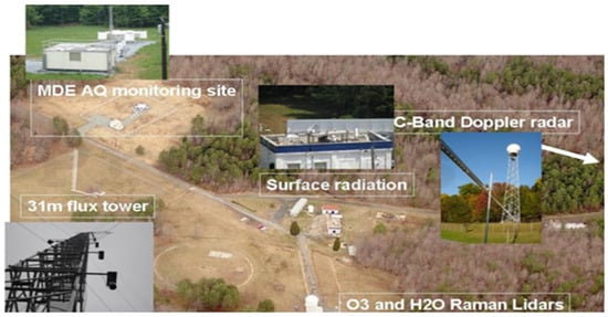
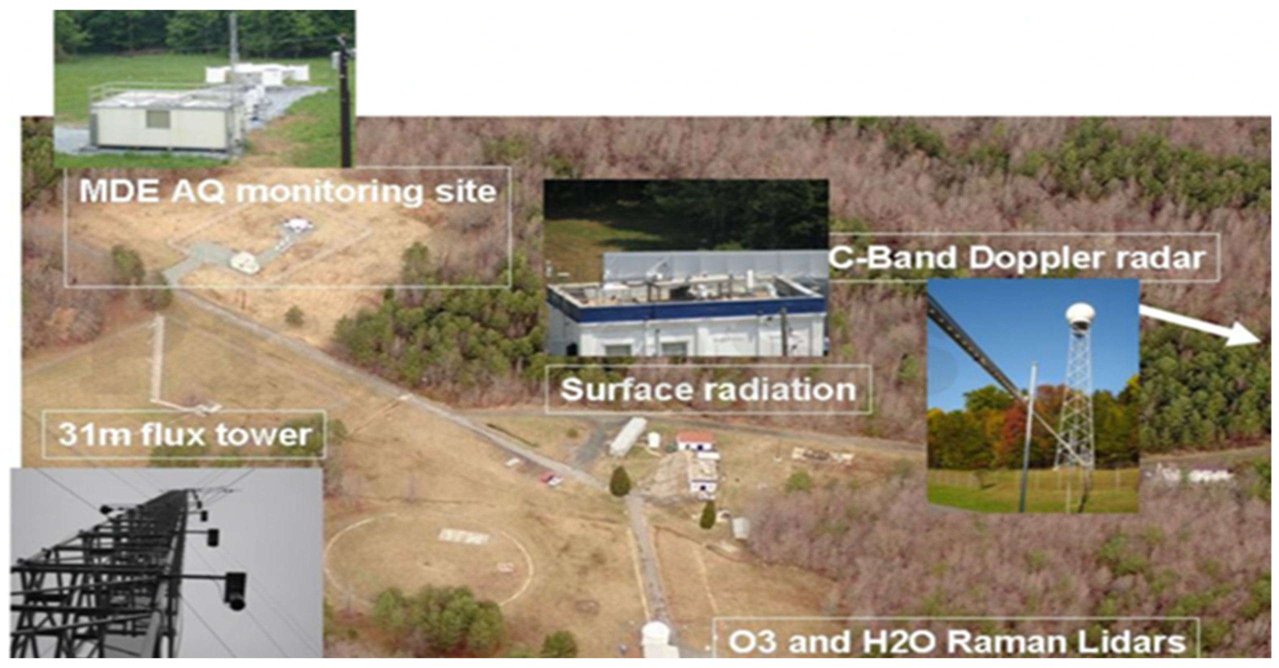
The Howard University Beltsville Campus (HUBC) Research Center is located 19 km northeast of downtown Washington, DC, spanning 110 acres (44.5 ha) of largely undeveloped land. The center has experimental facilities, including flux and meteorological towers, upper air sounding systems, spectral and broadband radiometers, gas analyzers, and particle sampling equipment (cf. Figure 1). HUBC collaborates on several projects with organizations such as NASA, NOAA, NGA, and the Maryland Department of Environment (MDE).
Figure 1.
HUBC ground-based testing facility. From the Howard University Beltsville Research Center.
2.2. Aeris Technologies MIRA Strato LDS CH4 and C2H6 Analyzer
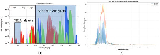
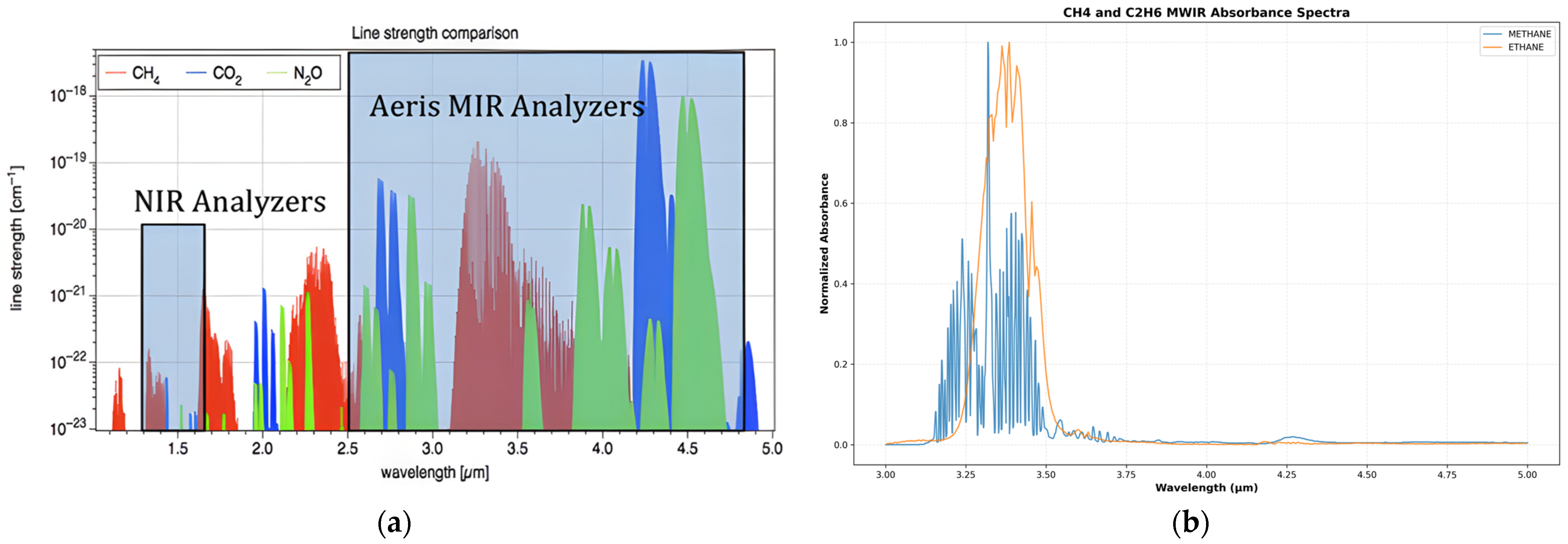
The Aeris Technologies MIRA Strato Leak Detection System (LDS) methane and ethane gas analyzer (Aeris Technologies, Inc., Hayward, CA, USA) is a multipass cell and laser absorption spectrometer with built-in GPS capabilities. The Strato LDS operates in the MWIR region, with a sensitivity of <1 ppb/s for CH4 and 500 ppt/s for C2H6, and is compatible with most commercial drones weighing at 2 kg [36]. MWIR absorption spectroscopy uses high-resolution tunable lasers to directly measure light absorption by gas molecules at specific wavelengths [37]. This method is effective because many gases, including methane and ethane, have strong and distinct absorption features in this region (cf. Figure 2), allowing for precise identification and quantification.
Figure 2.
A comparison of methane (CH4) absorption features. (a) Illustration of the spectral collection window of the MIRA Strato analyzer, which operates in MWIR to leverage the strong absorption of ethane (C2H6) for biogenic/thermogenic discrimination from aerissensors.com (accessed on 7 May 2025). (b) Corresponding normalized MWIR absorbance spectra of CH4 and C2H6 from NIST, demonstrating the spectral region used by the MIRA Strato analyzer.
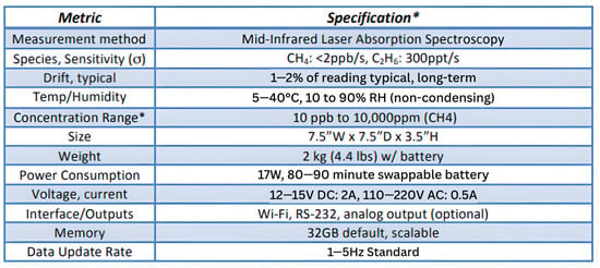
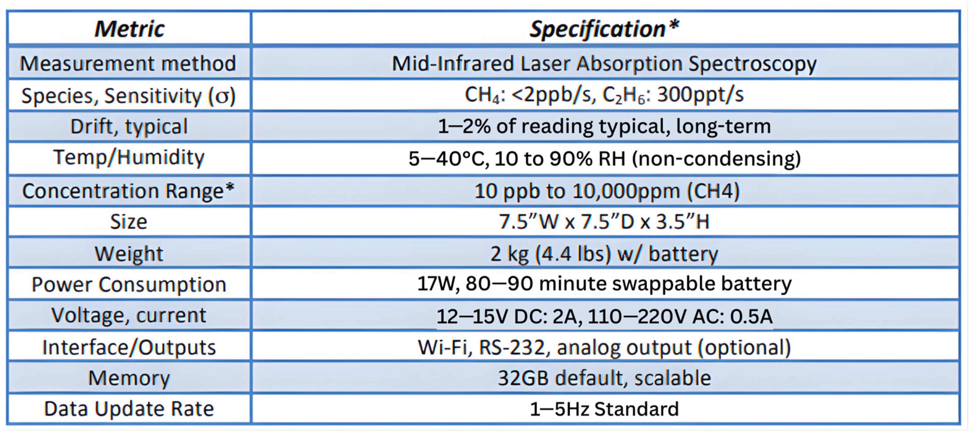
The MIRA Strato is equipped to discriminate thermogenic and biogenic CH4 emissions through its 13-m optical path length and 60 cm3 (60 mL) multipass cell technology. By folding the laser beam multiple times within the cell, the device maximizes the interaction between light and gas molecules, significantly amplifying the absorption signal without increasing the instrument’s physical size [38]. The analyzer internally measures gas concentrations at rates up to 1–5 Hz; these high-frequency readings are averaged and logged at one-second intervals [36], yielding stable time-aligned CH4 and C2H6 readings suitable for drone-based plume detection, as shown in Figure 3.
Figure 3.
MIRA Strato LDS methane sensor specifications. * Optional ranges, etc., can be configured for specific applications. From aerissensors.com.
Configuration and collection of methane measurements proceeded as follows [37]: The MIRA Strato was powered on 10–20 min before deployment to boot, ensuring proper GPS connection, and collected at a one-second duration. Data collection includes:
- An ‘engineering’ text file designed as an exhaustive repository of all the measurement parameters and results.
- Measured spectra in ASCII format (named ‘spectra-lite’) to diagnose issues or postprocess measurements.
- A KML file that is read directly on Google Earth to map gas concentrations and ethane-to-methane correlations.
2.3. Picarro G2301 CO2 and CH4 Analyzer
The Picarro G2301 (Picarro, Inc., Santa Clara, CA, USA) gas concentration analyzer is a Cavity Ring-Down Spectrometer (CRDS) that collects carbon dioxide (CO2) and methane (CH4) at parts-per-billion (ppb) and water vapor (H2O) at percent volume mixing ratio (%) [39]. CRDS is an ultra-sensitive laser absorption technique that uses highly reflective mirrors to trap light pulses in a cavity, resulting in effective path lengths of up to tens of kilometers to detect absorption [40]. Picarro analyzers increase their signal-to-noise ratio using a three-mirror cavity to support continuous traveling light waves [41]. The three-mirror configuration allows for laser light to circulate throughout the cavity, providing a longer path length and amplifying the absorption signal to detect even trace gas levels at the ppb and ppm range [39]. When the laser is turned off, the light within the cavity continues to bounce between the mirrors, gradually decaying due to the reflectivity loss known as ‘ring down’. In the presence of a target gas, additional absorption occurs, accelerating the ring-down time. This further increases the analyzer’s accuracy by comparing the ring-down time with and without the target gas. The G2301 has a response time of approximately 2.5 s and offers high measurement precision with a CH4 sensitivity of ±1 ppb over 5 s, improving to ±0.5 ppb over 5 min and ±0.3 ppb over 60 min [39]. These features make the G2301 well-suited for continuous monitoring and high-precision atmospheric research applications.
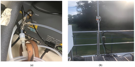
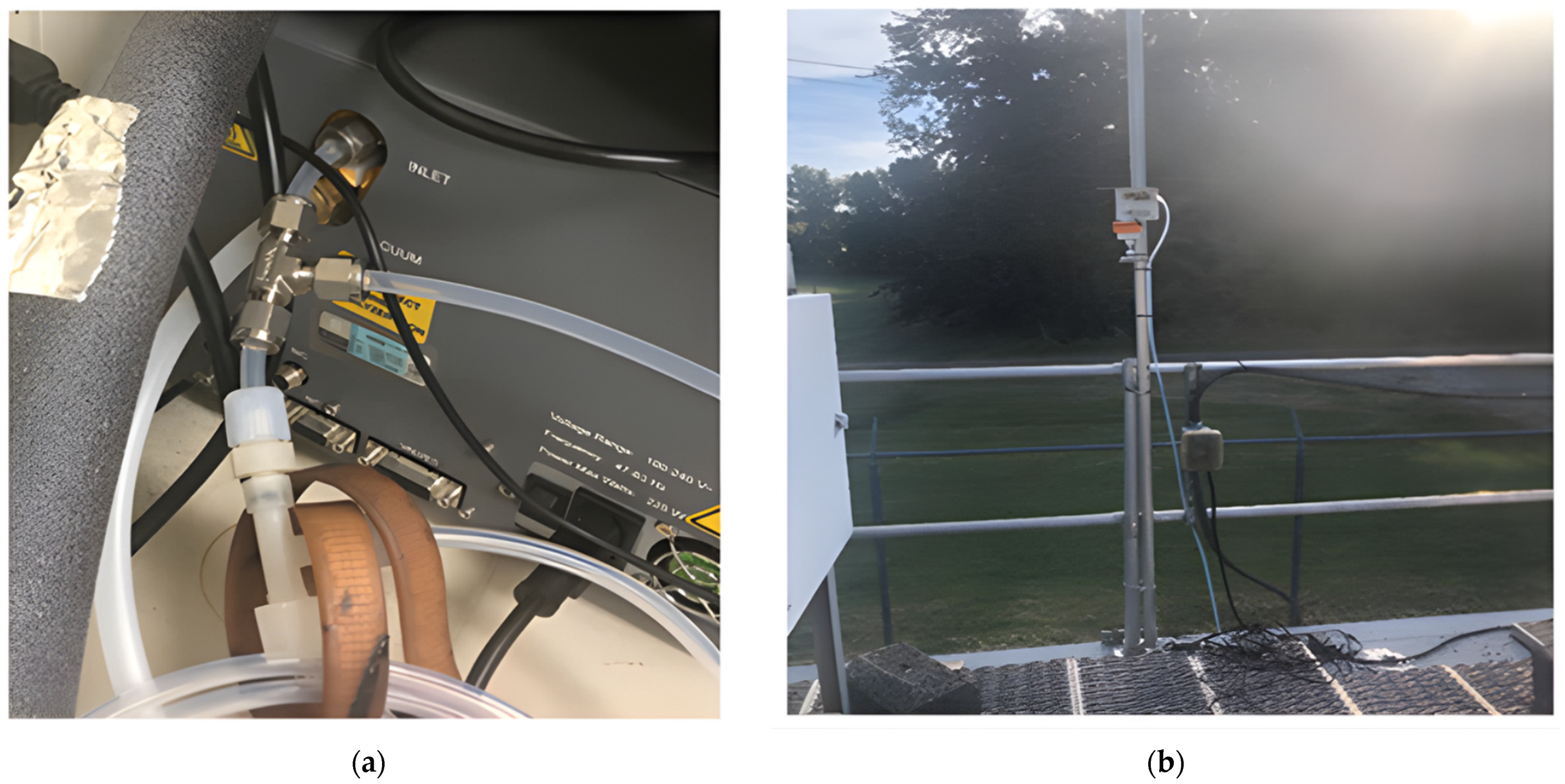
The G2301 was used to perform an intercomparing analysis with the MIRA Strato during the study. Both instruments were placed at the MDE Air Quality monitoring station in the northwest portion of the HUBC research center. The two-week analysis from 5–21 September 2023, was conducted to assess the MIRA Strato measurement consistency and accuracy. Instruments were connected via a shared tubing outlet, allowing for simultaneous measurements (cf. Figure 4). A Raspberry Pi single-board computer was connected to the serial port as a backup for power disconnection. The tubing outlet was lastly positioned on the station’s roof to collect measurements.
Figure 4.
Photographic documentation of the MIRA Strato intercomparison with the Picarro G2301 conducted at HUBC in September 2023. (a) Inlet tubing configuration connecting the MIRA Strato and Picarro G2301 analyzers to a shared ambient intake line. (b) Tubing outlet positioned on the rooftop of the HUBC MDE monitoring site, demonstrating the shared ambient air intake configuration for comparative analysis.
2.4. DJI Matrice 600 Pro Drone
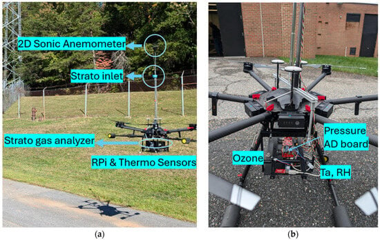
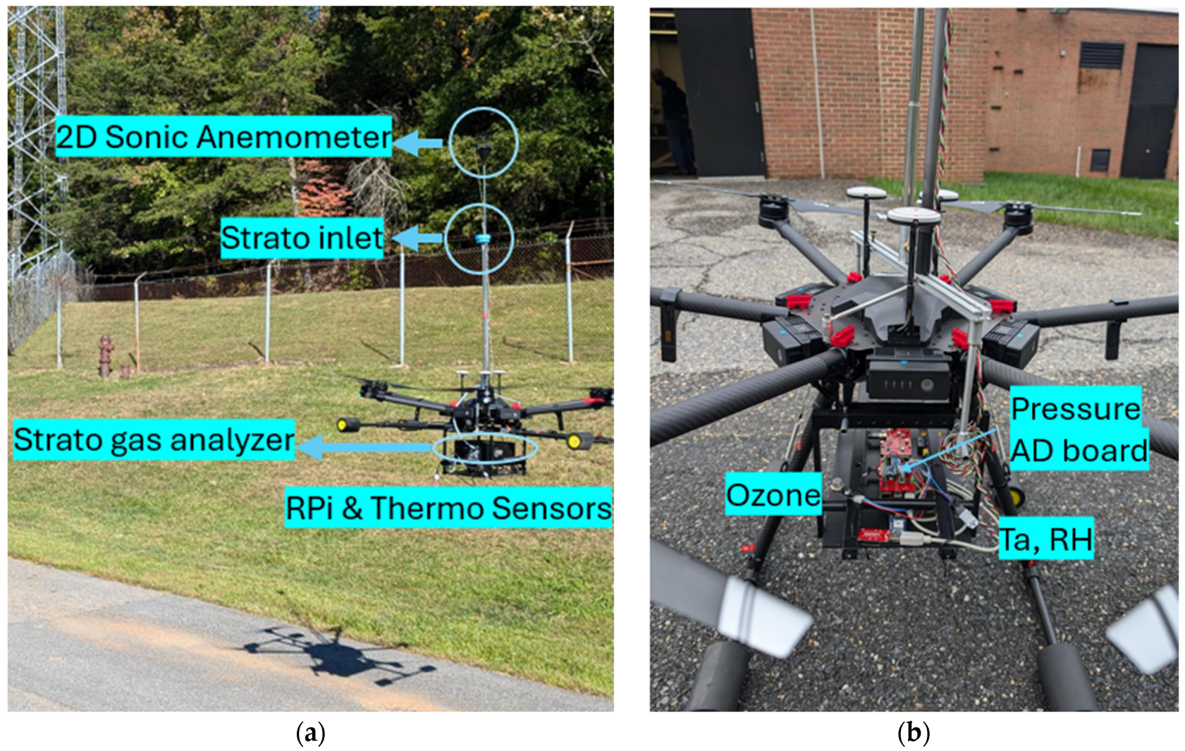
The DJI Matrice 600 Pro is a rotary-wing hexacopter drone weighing 9.5 kg (with six TB47S batteries), with a hovering span of 32 min (without payload), and a 6 kg maximum payload capacity [42,43]. The drone has the A3 Pro flight control system for enhanced stability and precision during atmospheric measurements [43]. During stationary hover, the aircraft uses GPS-based position-hold (DJI P-GPS) with a typical accuracy of ±0.5 m vertically and ±1.5 m horizontally under normal satellite reception. While the platform has a maximum ceiling height of 4.5 km, our operations were conducted below 120 m due to drone operating licensing limitations and payload considerations. According to the manufacturer (DJI Matrice 600 Pro user manual), the platform has a maximum wind resistance of 8 m/s and maximum ascent and descent speeds of 5 m/s and 3 m/s, respectively. Payload testing was conducted with a replica model of the Aeris Strato to determine a flight duration of 16–20 min, depending on the windshear. To optimize measurement accuracy and reduce down-washing effects, an 82.5 cm vertical inlet tube was installed above the propellers with a filter added to the opening to prevent particle contamination (cf. Figure 5). Previous fluid dynamic simulations determined that the Matrice 600 Pro series downwash disturbances decrease at a height of 60 cm above the body [27,29]. While this inlet configuration follows established best practices for mitigating downwash effects reported in literature [27,29], a direct comparative evaluation with and without the inlet extension was not conducted during payload testing. As a result, the effectiveness of the inlet design in reducing downwash-related sampling bias in this study is inferred from prior studies rather than quantitatively verified.
Figure 5.
DJI Matrice 600 Pro drone with inlet tubing during payload testing. (a) Placement of the MIRA Strato gas analyzer, inlet, and Raspberry Pi sensor. (b) Additional features of the drone include an anemometer, ozone, pressure, and temperature sensors.
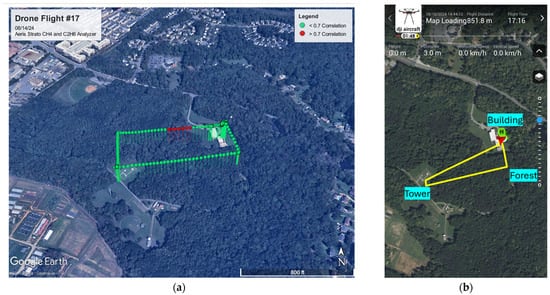
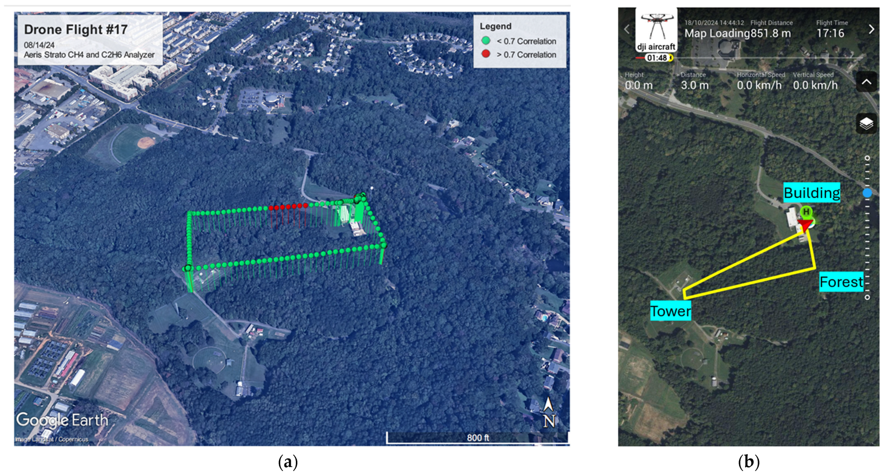
Flights were conducted during midday hours, typically starting at 13:20 local time with durations ranging from 17 to 20 min. This timeframe was selected to coincide with the afternoon TROPOMI satellite overpass and peak atmospheric mixing within the boundary layer. Compared to stable nighttime conditions, midday flights allow for greater vertical methane dispersion and reduce the influence of near-surface accumulation, resulting in more representative spatial sampling [44]. Vertical profile measurements were taken at several heights, including 25, 50, 75, 100, and 115 m above ground level, and across different environmental backgrounds such as above HUBC’s north building at 6 m structure height, forest canopy at 20–25 m height, and over a meteorological flux tower at 30 m structure height. Stable hovering at the given heights allowed us to record reliable measurements at each level. Flight paths were tracked using the MIRA Strato’s KML configuration system, enabling spatial analysis of ethane-to-methane Pearson correlation coefficients in areas likely influenced by biogenic or thermogenic sources (cf. Figure 6). Data points were color-coded: green for correlation coefficients < 0.7, and red for values ≥ 0.7. Elevated correlation zones (≥0.7) may indicate potential areas of high natural gas concentration [36].
Figure 6.
Example of flight path from deployments, with ethane-to-methane correlations, at HUBC using the MIRA Strato (a). Example of flight path (yellow line), derived from the DJI Matrice 600 Pro drone during the campaign, covering various environmental backgrounds within the area of interest, including buildings, forest, and the meteorological flux tower at HUBC (b).
A total of 14 flights were completed between October 2023 and September 2024 under varying meteorological conditions, as detailed in Table 1. The measurement strategy incorporated vertical profiling at consistent altitude intervals, weather condition monitoring to ensure safe operation, and real-time data logging through Strato’s streaming capability.
Table 1.
Flight collection dates, times, duration, altitudes reached, and observations.
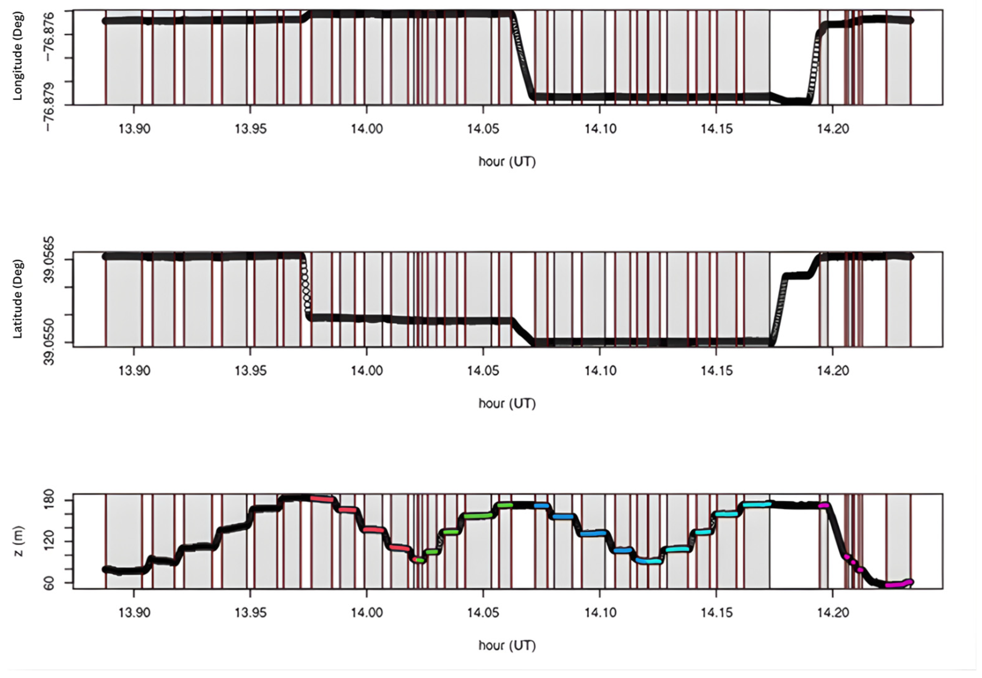
For each profile, the UAV hovered at the specified heights and environmental backgrounds for approximately 5 min. The flight path began at the north building, then proceeded to the forest site, and finally to the meteorological flux tower. At each location, ascending and descending measurements were taken. CH4, C2H6, and H2O concentrations were recorded, with averages, standard deviations, and sample sizes calculated from hovering levels (HL) based on the pressure time series as seen in Figure 7.
Figure 7.
Time series to determine the period for each HL. The top figure shows longitude, the second is latitude, and the last is height derived from the pressure sensor. The shaded areas correspond to the HL, and the colors indicate the profile location: black for ascending building, red for descending forest, green for ascending meteorological tower, blue for ascending forest, cyan for ascending tower, and magenta for descending building.
3. Results
3.1. Intercomparing Analysis
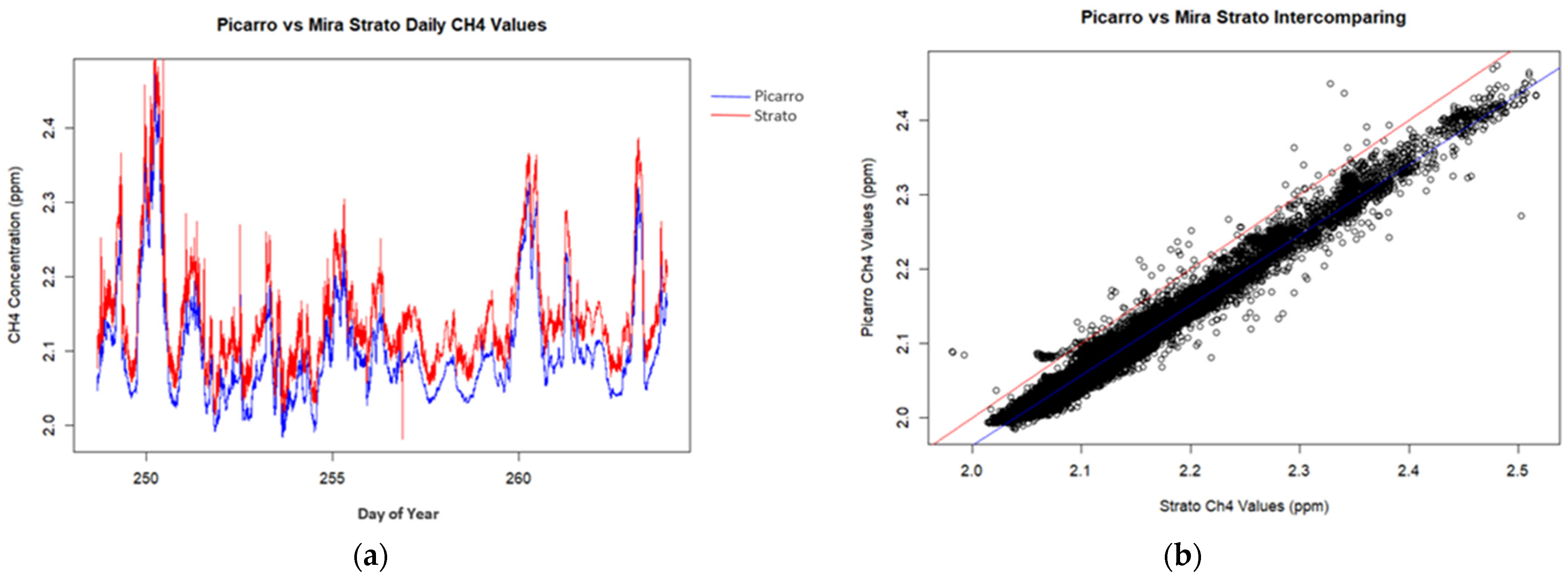
Intercomparing analysis with the Picarro G2301 methane analyzer revealed a correlation with an R2 value of 0.9845, indicating a near-perfect linear relationship between the two analyzers. Regression analysis showed a slope of 0.9438 and an intercept of 0.0750, demonstrating minimal systematic differences in methane concentration measurements (cf. Figure 8).
Figure 8.
Intercomparison results: daily values and linear regression. (a) Time series of CH4 concentrations (ppm) showing diurnal variability captured by both instruments, with strong agreement in temporal patterns. (b) Linear regression of paired CH4 observations indicating high correlation between MIRA Strato and Picarro (R2 = 0.9845, slope = 0.9438).
3.1.1. Hourly Analysis
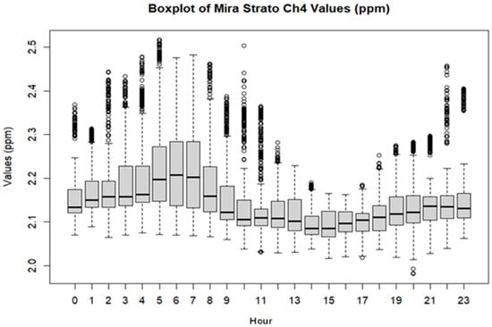
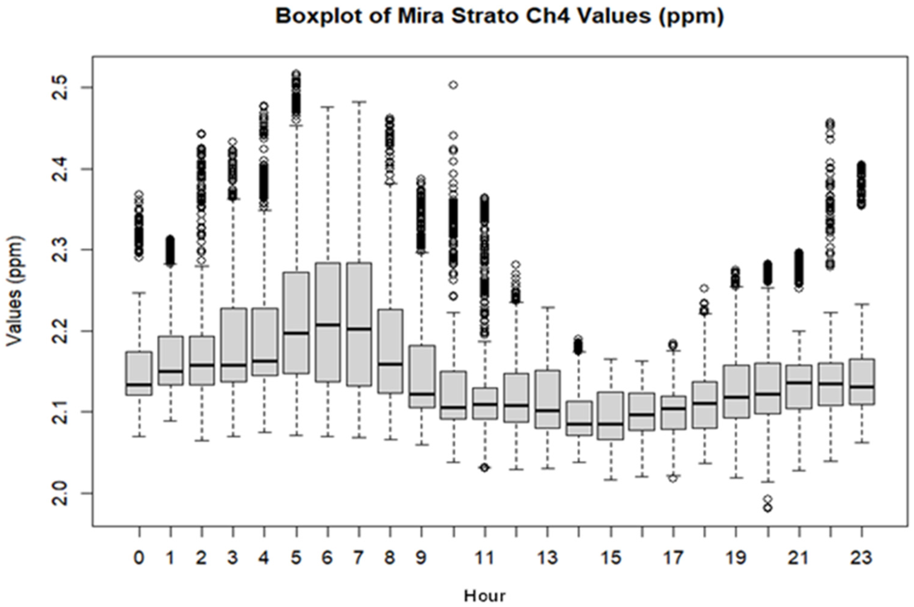
Diurnal evaluation determined a high median concentration at HUBC during sunrise between 04:00 and 08:00 LT, reaching approximately 2.2 ppm. The lowest median concentrations occurred during afternoon hours around 13:00–17:00 LT, dropping to about 2.1 ppm (cf. Figure 9). The morning peak is consistent with the expected boundary layer behavior, suggesting surface accumulation with little atmospheric mixing during stable nighttime conditions. On the other hand, the late afternoon drop in concentration is associated with increased vertical mixing and convection, boundary layer growth, and solar heating.
Figure 9.
MIRA Strato hourly concentrations during the 2023 intercomparing analysis. Boxplots represent hourly distributions (00:00–23:00 LT), highlighting elevated median CH4 levels during early morning hours (04:00–08:00 LT) and lower values during afternoon periods (13:00–17:00 LT), consistent with boundary layer dynamics and convective mixing. Whiskers denote 1.5× the interquartile range, and individual points represent outliers, suggesting infrequent enhancement events.
There are several outliers, especially in the late night and early morning, with some spikes as high as 2.5 ppm. The widest interquartile range is also in the morning peak, reflecting greater methane concentration variability. The larger change would likely be due to the stable nighttime conditions giving way to daytime mixing. During the afternoon (13:00–16:00 LT), concentration ranges are lower and less variable, consistent with improved mixing under unstable weather conditions.
3.1.2. Daily Analysis
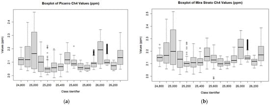
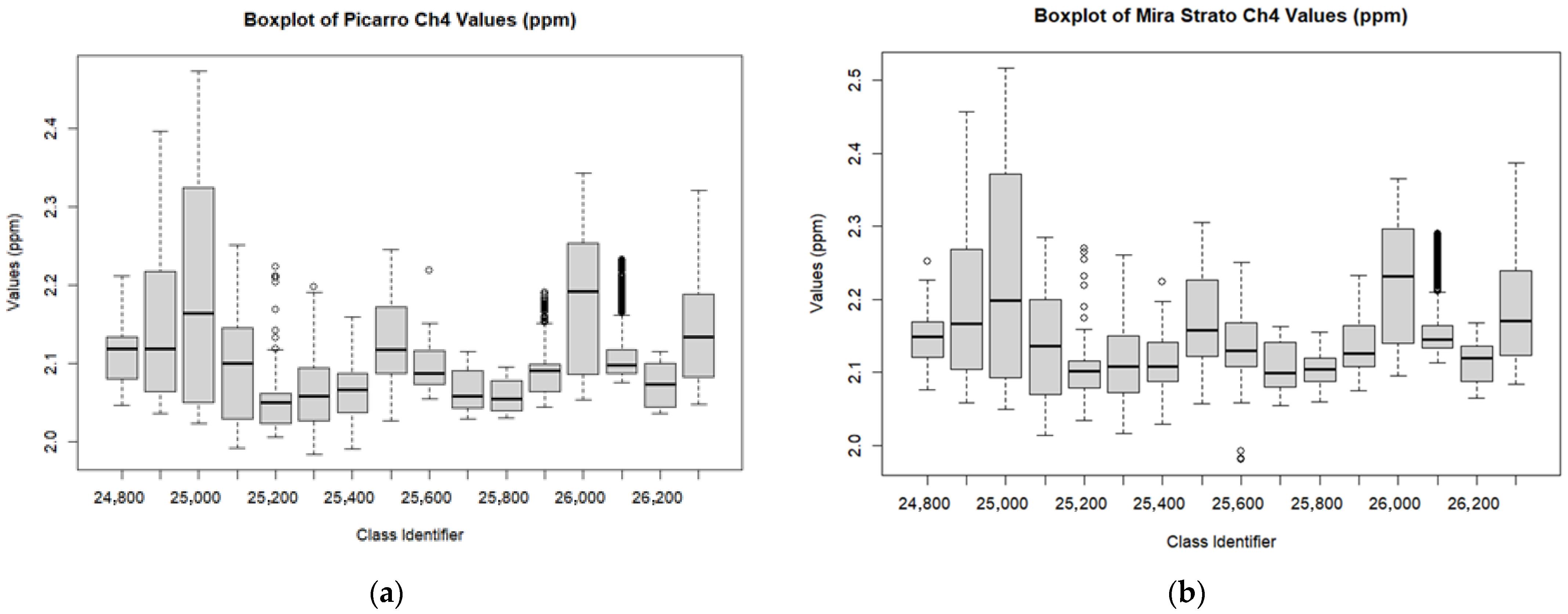
Daily variation during the intercomparing analysis showed strong agreement between the MIRA Strato and Picarro G2301 analyzers. The highest median concentrations reached 2.15–2.16 ppm for the Picarro and 2.19–2.20 ppm for the MIRA Strato, with upper quartile values extending to 2.30 ppm and 2.37 ppm, respectively. The lowest median concentrations displayed similar trends at 2.05–2.08 ppm for the Picarro and 2.10–2.08 ppm for the MIRA Strato. Corresponding upper quantile concentrations ranged from 2.10–2.12 ppm and 2.15–2.18 ppm, respectively. Overall, both instruments tracked daily methane trends closely, with the MIRA Strato reporting slightly higher values in the upper quantile range (cf. Figure 10).
Figure 10.
Boxplot comparing daily methane (CH4) fluctuation measured by (a) the Picarro G2301 and (b) the MIRA Strato analyzer during the 2023 intercomparing analysis. The class identifier represents day of year. The plots illustrate similar day-to-day variability and overall agreement in diurnal CH4 trends, with the MIRA Strato capturing comparable distributional patterns, including median values and dispersion. Whiskers denote 1.5× the interquartile range, and individual points represent outliers, suggesting infrequent enhancement events.
3.2. MIRA Strato Gas Chamber Calibration
Calibration was completed at the NOAA Air Resources Laboratory (ARL) in College Park, MD, with collaboration from NOAA, the University of Maryland, and Howard University. The calibration process involved multiple flow rates, theoretical set points, and statistical analysis to evaluate the MIRA Strato’s accuracy in measuring methane (CH4) and ethane (C2H6). The calibration protocol followed NOAA ARL procedures, with gas standards selected to represent typical ambient methane and ethane concentrations and available tank specifications. Gas standards included a Matheson C2H6 standard at 4.83 ppm (±2% accuracy), and three CH4 standards at approximately 1929, 2222.7, and 3152 ppb. Methane standards were introduced directly into the sample line without dilution. Two mass flow controllers (MFCs) were used to regulate the flow rates of C2H6 calibration gas and zero air, with the zero-air flow fixed at 2 standard Liters per minute (SLPM) and ethane flow varied from 0 to 10 Standard cubic centimeters per minute (SCCM). Data collection also involved measuring the instrument’s response at various voltage set points, ranging from 0 to 5 V, corresponding to the ethane flow range of 0–10 SCCM. Both MFCs were calibrated using two Mesa Labs Definer 220 flow calibrators with ±1% accuracy.
Calibration results for methane, as detailed in Table 2, revealed a strong linear relationship, with a slope of 0.9678, and y-intercept of 45.966, yielding an R2 value of 0.9986, which indicates high measurement consistency. Similarly, ethane displayed a slope of 1.0111 and a y-intercept of 8.04816, with an R2 value of 0.9879. The F-statistics and residual sums of squares for both gases were also within acceptable ranges, validating the MIRA Strato’s precision across varying concentrations and conditions.
Table 2.
MIRA Strato’s gas chamber calibration linear regression using gas standards from NOAA ARL. Results indicate high measurement accuracy, with a R2 value of 0.9986 across varying SRM’s.
3.3. Ambient Methane Profiles from UAV Observations
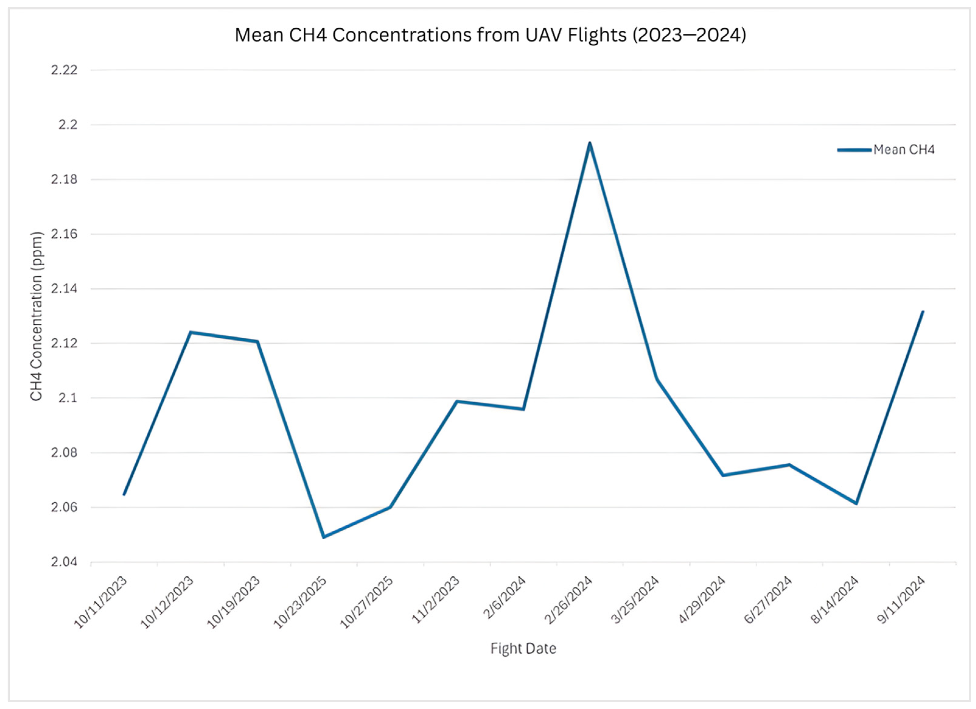
Across the 14 flights, mean concentrations displayed standard urban ambient levels ranging from 2.05 to 2.19 ppm. Standard deviations remained consistently under 0.02 ppm, pointing toward both precise measurements and stable background methane levels. The highest average concentration was observed at 2.19 ppm on 26 February 2024, while the lowest occurred on 23 October 2023, at 2.05 ppm. Peak values reached 2.23 ppm in late April, and the lowest single reading was 2.02 ppm on 23 October (cf. Figure 11). Throughout all flights, temperatures varied widely, from a low of 12.3 °C in the winter to a high of 32.9 °C in summer flights.
Figure 11.
Mean methane (CH4) concentrations measured using the MIRA Strato analyzer during 14 UAV flights conducted between October 2023 and September 2024.
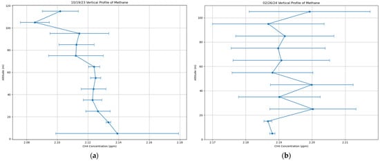
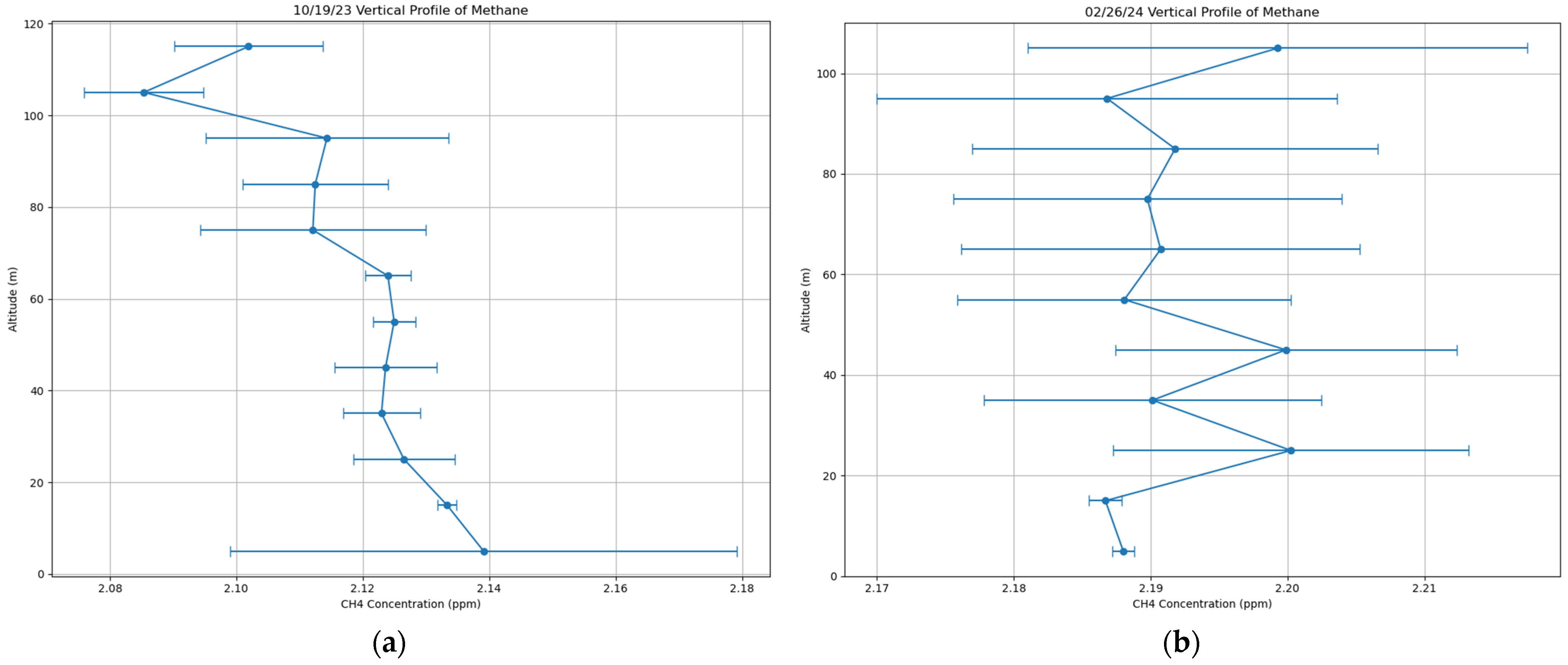
Flight altitudes ranged between 10 and 117 m, separated into 10-m intervals for vertical profile analysis. Weather conditions, especially temperature inversions, had a noticeable effect on methane patterns. As shown in Figure 12, during the October 19 flight, methane concentrations were highest (2.139 ppm) near the ground (0–10 m) and dropped off with altitude, suggesting that stable air trapped methane close to the surface. In contrast, on 26 February, methane levels actually increased with height—from 2.187 ppm at 0–10 m to 2.199 ppm at 100–110 m—hinting that methane from nearby sources was being advected at that level. Some flights, like the one on 25 October, showed nearly uniform methane concentrations (2.171–2.167 ppm) from 0 to 115 m, indicating well-mixed air. Winter and fall flights displayed more frequent occurrences of surface-enhanced methane due to possible shallow or stable boundary layers with higher overall concentrations (2.188–2.199 ppm). In contrast, summer flights (June–August 2024) displayed more uniform methane distribution (around 2.060–2.080 ppm) throughout the measured altitudes, a sign that stronger summer mixing was spreading methane more evenly through the atmosphere.
Figure 12.
Vertical profiles for 19 October 2023, and 26 February 2024. (a) 19 October displayed variable methane concentrations near ground (0–10 m), suggesting ground level accumulation; (b) 26 February displayed higher fluctuations throughout, with concentration increases with altitude.
3.4. Ethane Co-Tracer UAV Observations and Anomalies
Ethane concentrations as a source apportionment co-tracer, ranged extensively throughout the flight campaign from below detectable because of instrument constraints to as much as greater than 19.41 ppb. A previous study using the Aeris Technologies MIRA Ultra indicates artifacts in ethane readings when sampling dry air with low water vapor content (below 1.05% H2O) [45]. This is due to MIRA lasers’ reliance on water absorption features for wavelength calibration. Under low humidity conditions, the absence of water vapor can cause the laser to lose its frequency lock [45], thus leading to inconsistent measurements (ranging from negative to positive). This is particularly critical in diffuse ambient measurements where single plume concentrations are not available to dominate the signal.
During this study, we believe negative values were attributable to baseline drift and response noise near detection limits. MIRA Strato specifications report a detection threshold of 500 parts per trillion per s (ppt/s) ≈ 0.5 ppb for ethane [36], with low concentrations or ambient measurements fluctuating below zero. Excluding these anomalies, concentrations were extremely variable with means between 2.37 and 8.16 ppb on individual flights, and no temporal, seasonal, or spatial patterns were apparent in the ambient measurements.
3.5. Influence of Hovering Environments on Vertical Gas Profiles
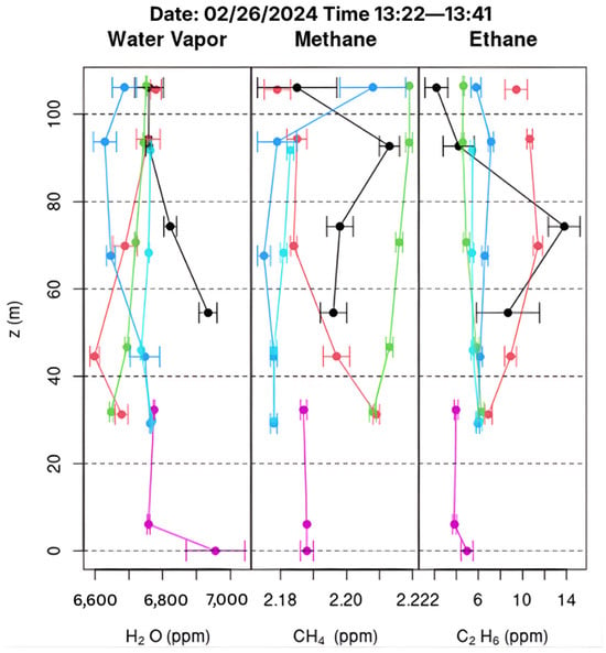
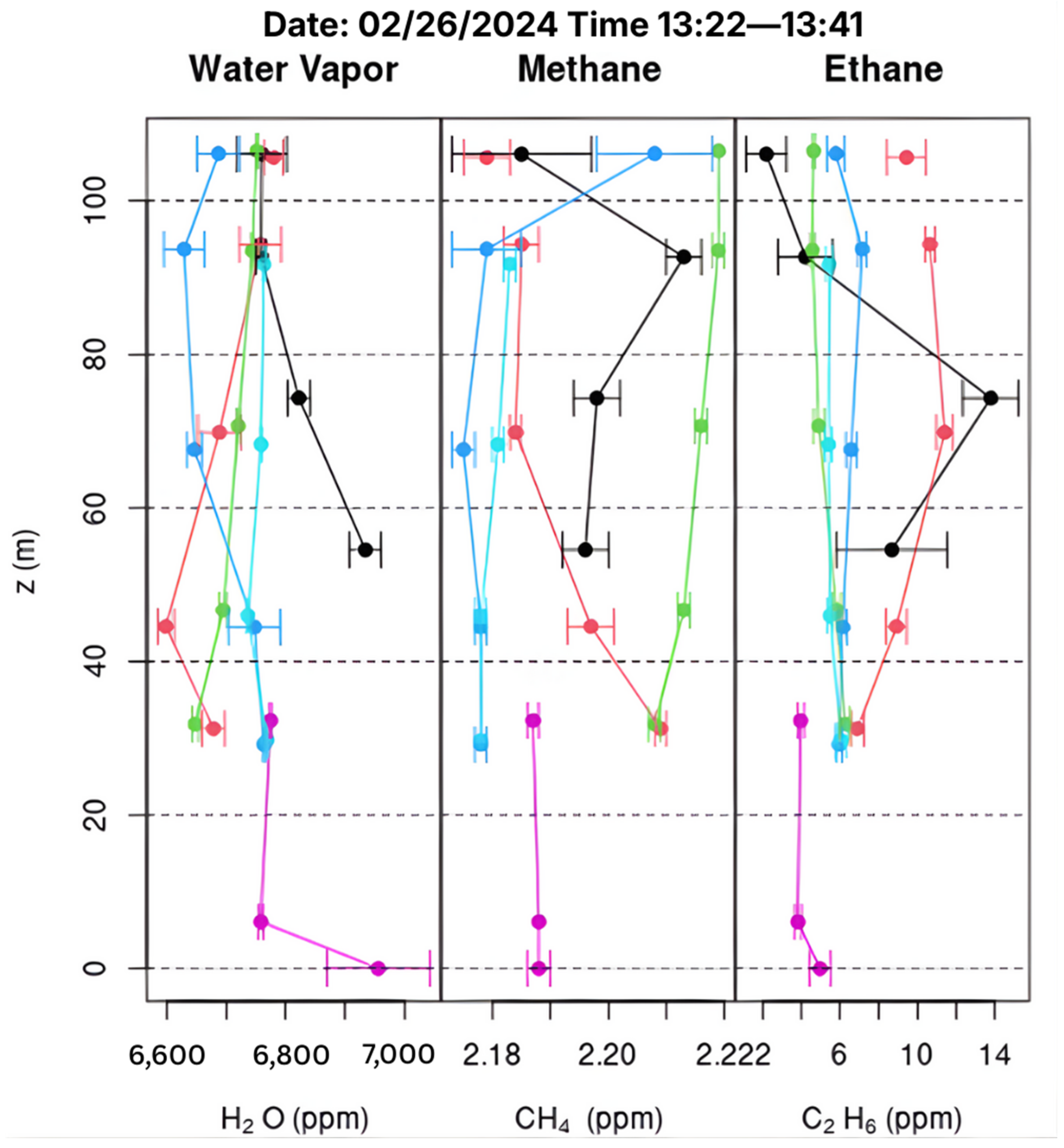
Analyzing the vertical distribution of CH4, C2H6, and H2O concentrations across different hovering environments during UAV flights, based on height parameters defined in Section 2.4, revealed distinct boundary-layer behaviors and the influence of surface interactions. Across all flights, vertical profiles varied modestly by environment but showed consistent overall structure. Methane levels increased during the ascent and descent of HBCU’s north building. The building ascending showed a median of 2.098 ppm (mean: 2.114 ± 0.018 ppm), and the building descending showed 2.079 ppm (mean: 2.095 ± 0.023 ppm), indicating a micro-emission influence. In contrast, forest (2.083–2.091 ppm median) and tower coverage (2.077–2.084 ppm median) displayed smoother profiles typical of a convective boundary layer. Notably, ascents over the meteorological tower often reached the upper range of observed methane values, with tower ascending achieving the highest overall mean at 2.100 ppm; a pattern also visible in individual-day profiles such as 26 February 2024 (2.180 ppm; cf. Figure 13), which may indicate localized mixing or nearby plume recirculation around the tower structure.
Figure 13.
Vertical profiles collected on 26 February 2024, show distinct differences in trace gas structure associated with the hovering environment. Each profile includes ascending building (black), descending building (magenta), ascending forest (blue), descending forest (red), ascending meteorological tower (green), and ascending tower (cyan) flight segments.
Ethane exhibited the strongest environmental sensitivity, with higher near-surface values over the north building (mean: 2.19 ± 2.59 ppb ascending, standard deviation: 6.87 ppb) and lower, more uniform concentrations over the forest (mean: 0.62 ± 1.89 ppb ascending, standard deviation: 5.29 ppb). Unlike methane, ethane frequently exhibited localized perturbations, particularly around the meteorological tower, with measurable concentrations ranging from 0.19 to 8.63 ppb (standard deviation: 2.77 ppb–2.96 ppb across ascending and descending profiles), suggesting the influence of mechanical turbulence or horizontal plume advection. Water vapor showed the clearest gradients, driven primarily by meteorology rather than surface type, with low winter humidity averaging 4561 ppm (range: 3038–6956 ppm) and substantial summer increases averaging 17,272 ppm (range: 15,887–19,097 ppm) near the surface.
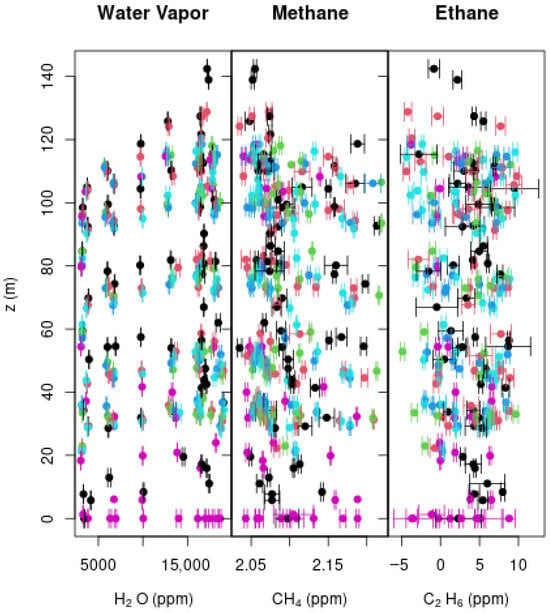
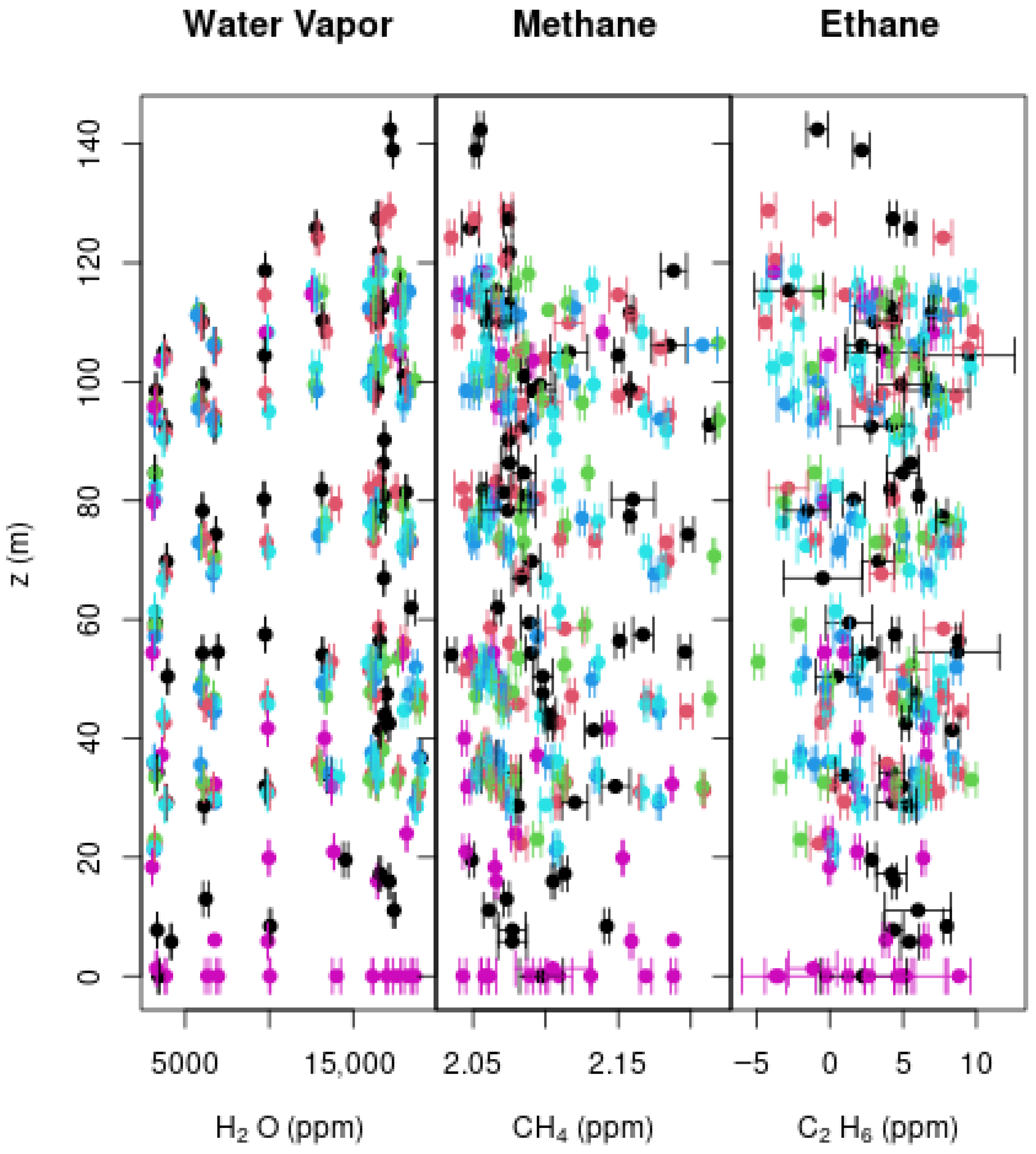
Minor systematic differences between ascent and descent traces were observed, particularly in building environments. Near-surface (z < 50 m) C2H6 concentrations were higher during building ascent (5.06 ± 5.41 ppb) compared to descent (1.59 ± 2.48 ppb), a difference of 3.47 ppb (p = 0.12), suggesting ascending measurements may capture fresher near-surface emissions before vertical mixing homogenizes the signal, though this difference did not reach statistical significance. Descending CH4 profiles showed no significant ascent-descent difference (p = 0.47) despite equipping the UAV with a tubing inlet to minimize downwash. Forest ascent and descent profiles were more consistent, likely due to stronger natural turbulence within the canopy, with the forest maintaining intermediate values between 2.052 and 2.219 ppm (standard deviation: 0.044–0.053 ppm) across measurement days. Coverage over the meteorological tower occasionally displayed mid-altitude deviations during ascent, which may reflect mechanical turbulence rather than true atmospheric gradients, as evidenced by ethane variability at the tower location (standard deviation: 4.22–4.93 ppb; cf. Figure 14).
Figure 14.
Aggregated vertical profiles of H2O, CH4, and C2H6 across all UAV flights, grouped by hovering environment. Colors denote ascending building (black), descending building (magenta), ascending forest (blue), descending forest (red), ascending meteorological tower (green), and ascending tower (cyan) flight segments.
3.6. Correlation Analysis
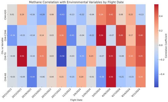
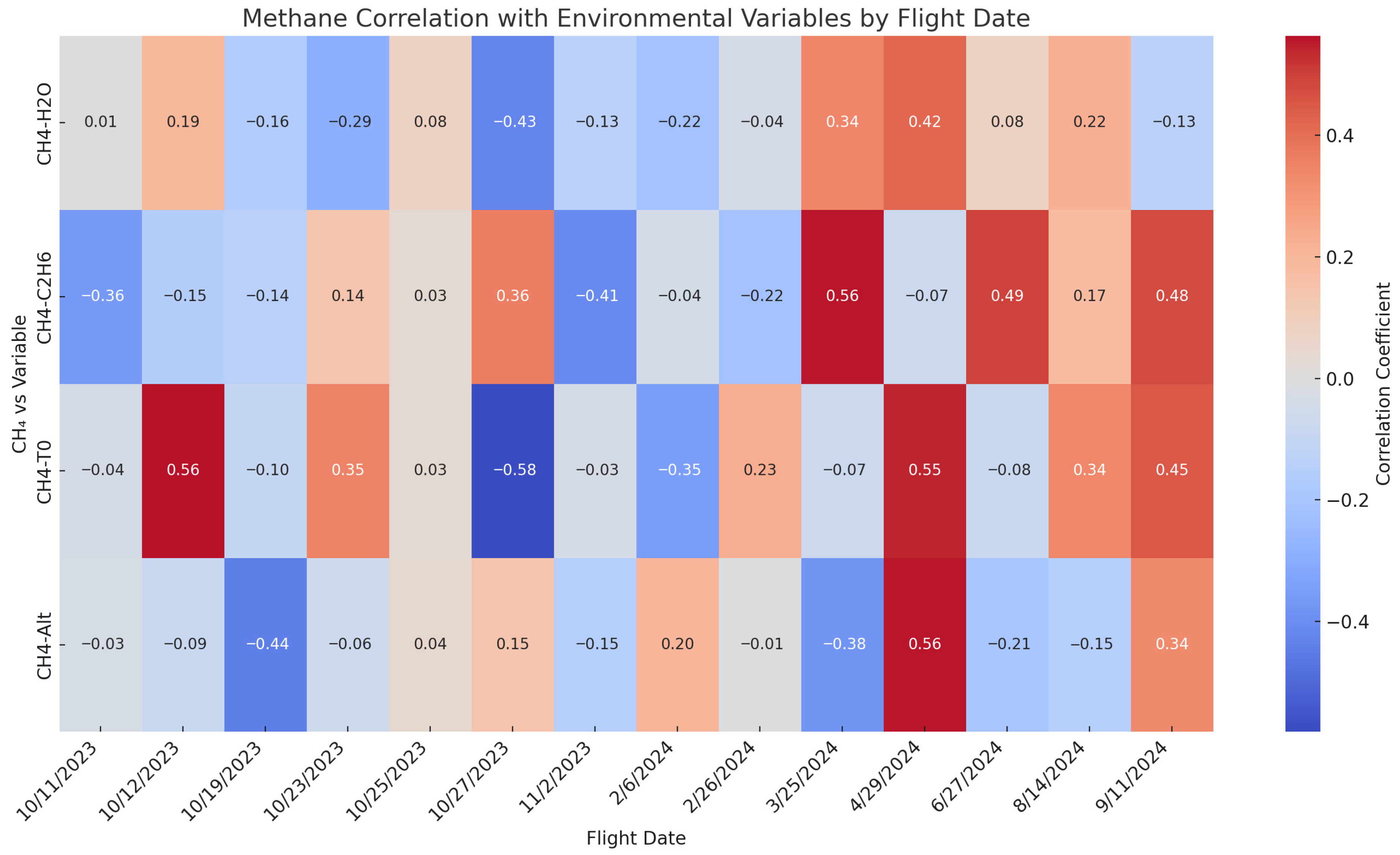
The correlation between methane and environmental variables provided insight into the behavior of methane sources and the atmospheric processes influencing concentrations (cf. Figure 15). Correlations between CH4 and H2O were weak and inconsistent, both negative and positive, suggesting a limited influence of humidity on methane variability or possible cross-sensitivity of the instrument. As noted above, CH4 and C2H6 correlations ranged from strong negative values (possibly artifactual) to moderate positive correlations (r = 0.36–0.56) suggestive of co-located thermogenic sources, though interpretation remains limited by established instrument constraints. CH4-temperature (T0) correlations varied in strength and direction, most likely reflective of boundary-layer dynamics, diurnal heating, and thermal stratification effects. Among all variables, temperature showed the strongest average correlation with CH4, followed by C2H6 and H2O. Altitude generally showed a negative correlation with methane, implying surface accumulation. However, positive correlations on certain days (e.g., 29 April) suggest vertical mixing or transport from a nearby source at higher elevations. These patterns reflect the analyzer’s sensitivity to temporal meteorological variability and validate its use in source attribution and boundary-layer transport characterization.
Figure 15.
Heatmap of Pearson correlation coefficients between CH4 concentrations and environmental variables (altitude, temperature, ethane, and water vapor) for each UAV flight. Warmer colors indicate stronger positive correlations, while cooler colors indicate stronger negative correlations.
3.7. Regression Analysis
To further evaluate the drivers of ambient methane variability across all UAV flights, we performed multivariate linear regression using temperature, altitude, and ethane as predictors. The regression coefficients differed widely among individual flights, indicating complex and inconsistent relationships without any clear seasonal trends.
3.7.1. Altitude Effects
Altitude coefficients showed high flight-to-flight variability with no consistent seasonal trend. As displayed in Table 3, several flights displayed surface accumulation with significant vertical gradients observed. For example, 19 October (slope = −3.05 × 10⁻⁴ ppm/m, p < 0.001) and 27 June (slope = −2.70 × 10⁻⁵ ppm/m, p < 0.001) flights were characterized by negative correlations, indicative of surface-based methane accumulation under stable boundary layer conditions. Few flights showed positive altitude correlation, consistent with convective transport (e.g., 6 February: 9.93 × 10⁻⁵ ppm/m, p < 0.001; 11 September: 1.50 × 10⁻⁴ ppm/m, p < 0.001). Two flights showed non-significant altitude effects (25 March: p = 0.904; 14 August: p = 0.351), suggesting well-mixed atmospheric conditions. Across the 14 flights, seven exhibited surface accumulations, four showed aloft enhancement, and three showed non-significant/well-mixed relationships during typical peak atmospheric mixing hours of 13:30–15:27 LT. This suggests that local emissions and meteorological variability conditions beyond diurnal mixing alone play a major role in methane’s boundary-layer vertical structure at the site.
Table 3.
Summary of vertical methane gradient regression results across UAV flights from October 2023 to September 2024. Each row represents the linear regression slope (ppm/m), coefficient of determination (r2), and p-value for the relationship between CH4 concentration and altitude.
3.7.2. Temperature Relationships
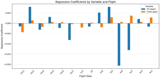
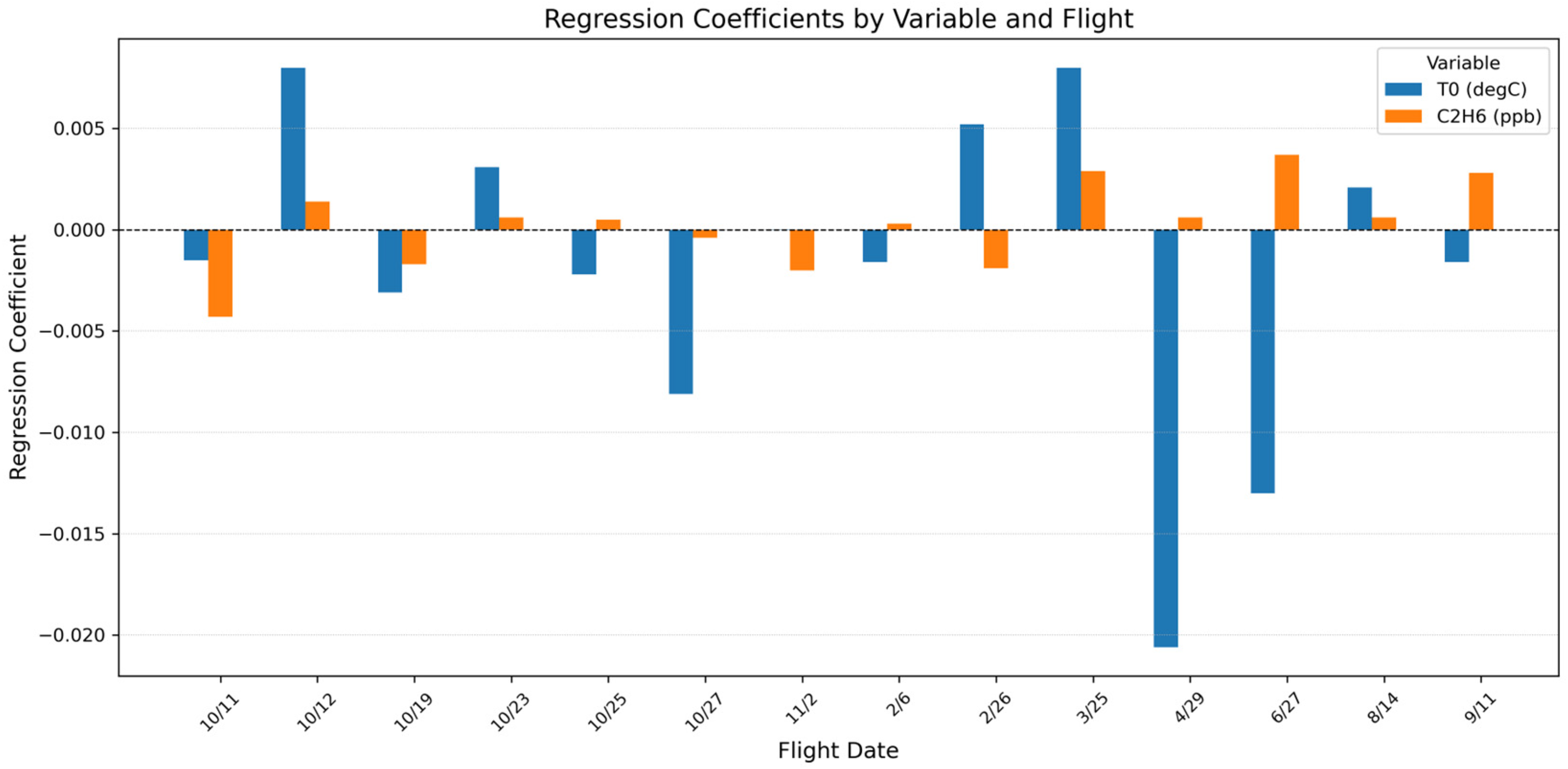
Temperature coefficients varied from strongly negative to moderately positive among flights, with the most negative coefficient in late spring (29 April: −0.021 ppm/°C, p < 0.001) and fall (27 October: −0.008 ppm/°C, p < 0.001). Positive temperature relationships were observed in both cool (12 October: +0.008 ppm/°C, p < 0.001) and warm seasons (25 March: +0.008 ppm/°C, p < 0.001), suggesting that temperature effects are driven by flight-specific atmospheric conditions rather than consistent seasonal processes.
3.7.3. Ethane Coefficients
Despite known instrumental limitations, ethane showed statistically significant coefficients across most flights, though with inconsistent patterns. For fall months, ethane specifically displayed strong negative coefficients (e.g., 11 October: slope = −0.0043 ppm, p < 0.001; 2 November: −0.002 ppm, p < 0.001), contrary to expectations of enhanced thermogenic emissions during heating season and most likely reflect instrumental artifacts. Positive ethane coefficients were found in warmer months (27 June: 0.0037 ppm, p < 0.001; 25 March: 0.0029 ppm, p < 0.001), possibly reflecting real thermogenic co-emissions, although interpretation is still constrained by measurement uncertainties (cf. Figure 16).
Figure 16.
Regression coefficient for temperature (blue) and ethane (orange) across 14 UAV flight dates. Ethane displayed a general positive trend across dates, while temperature varied substantially. The lack of a consistent pattern across dates highlights the influence of localized conditions, variable flight paths, and potential sensor behavior on observed methane concentrations.
3.8. Precision and Temporal Stability of Methane Observations
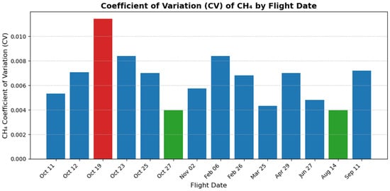
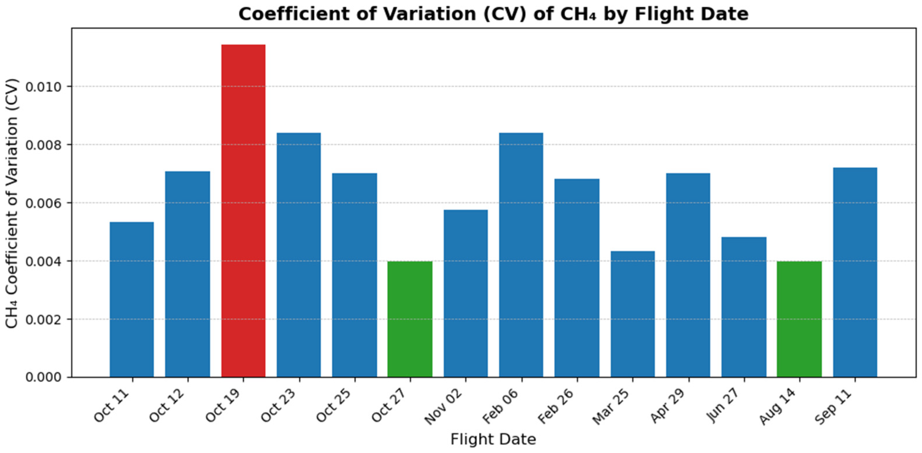
For each flight, the coefficient of variation (CV) of the CH4 concentration was determined to assess the MIRA Strato’s signal stability and variability under ambient conditions. CV values varied from 0.00397 to 0.01143 (mean CV ≈ 0.0067) in all 14 flights, indicating exceptionally low relative variability in measured concentrations. The highest CV was observed on 19 October (CV = 0.01143), coinciding with the strongest CH4–altitude gradient and negative regression coefficients for all predictors. This implies elevated stratification and sharper vertical CH4 gradients on that day, to which the analyzer was sensitive enough to detect. In contrast, late summer and fall flights such as 14 August (CV = 0.00398) and 27 October (CV = 0.00397) were less variable, likely reflecting stable atmospheric or instrument conditions (cf. Figure 17). These results highlight the sensor’s high precision in the field, with CV values consistently below 1.2%. This is well within acceptable limits for ambient methane analyzers according to instrument validation studies [46] and demonstrates MIRA Strato’s stable performance across varying environmental conditions and methane distributions.
Figure 17.
Coefficient of variation (CV) for CH4 concentration by flight date. Red bar indicates the highest observed CV (19 October 2023); green bars represent comparison flights (27 October 2023, and 14 August 2024); blue bars represent all other flights.
4. Discussion
The UAV-based methane monitoring campaign provided valuable proof-of-concept for microscale methane observations within the atmospheric surface layer. By deploying the Aeris Technologies MIRA Strato analyzer across 14 flights from October 2023 to September 2024 (7 Fall, 3 Winter/Spring, and 4 Summer), we assessed the field stability of the sensor, correlation with environmental drivers, and ability to capture ambient variability, including temporal, spatial, and atmospheric insights into near-surface CH4 behaviors and relationships.
The MIRA Strato analyzer exhibited strong performance in field and laboratory settings. The high signal-to-noise ratio enabled the detection of subtle ambient variations in CH4 and co-tracers regardless of in-plume concentrations. Despite some challenges with low-level C2H6 detection, the instrument captured consistent spatial patterns and correlation behavior that aligned with atmospheric expectations. The combination of precision, reproducibility, and spatial responsiveness confirms the analyzer’s robustness for UAV-deployed ambient methane research.
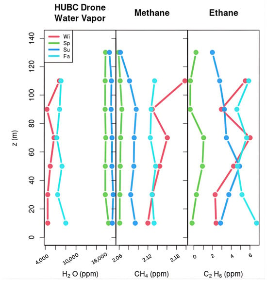
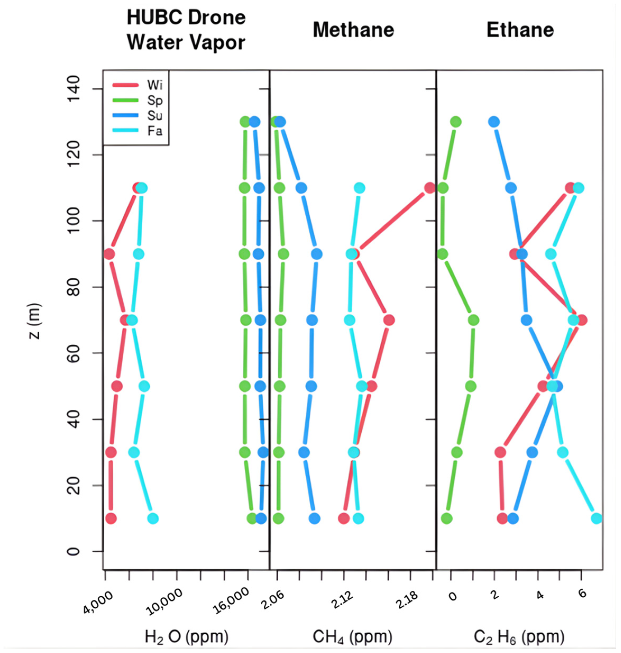
Although ambient levels throughout the campaign remained around ~2 ppm, concentrations showed seasonal behavior, with elevated concentrations in the fall and early winter (cf. Figure 18). Maximum CH4 concentrations were observed on 19 October at 2.23 ppm, consistent with expected seasonal shifts in atmospheric mixing. This date also exhibited the most stable conditions and surface accumulation according to the regression analysis. The lowest concentration was observed on 14 August at 2.03 ppm, which also corresponds to the CV value on this date, indicating elevated mixing. The second highest mean concentration (26 February) is not conclusive to seasonal trends but is likely attributable to localized emission influences.
Figure 18.
Seasonally averaged vertical profiles of H2O, CH4, and C2H6 derived from aggregated UAV measurements. Colors represent winter (red), spring (green), summer (blue), and fall (cyan). Methane shows a clear seasonal pattern, with higher concentrations during fall and winter and lower, tightly constrained values in spring and summer, consistent with seasonal emissions.
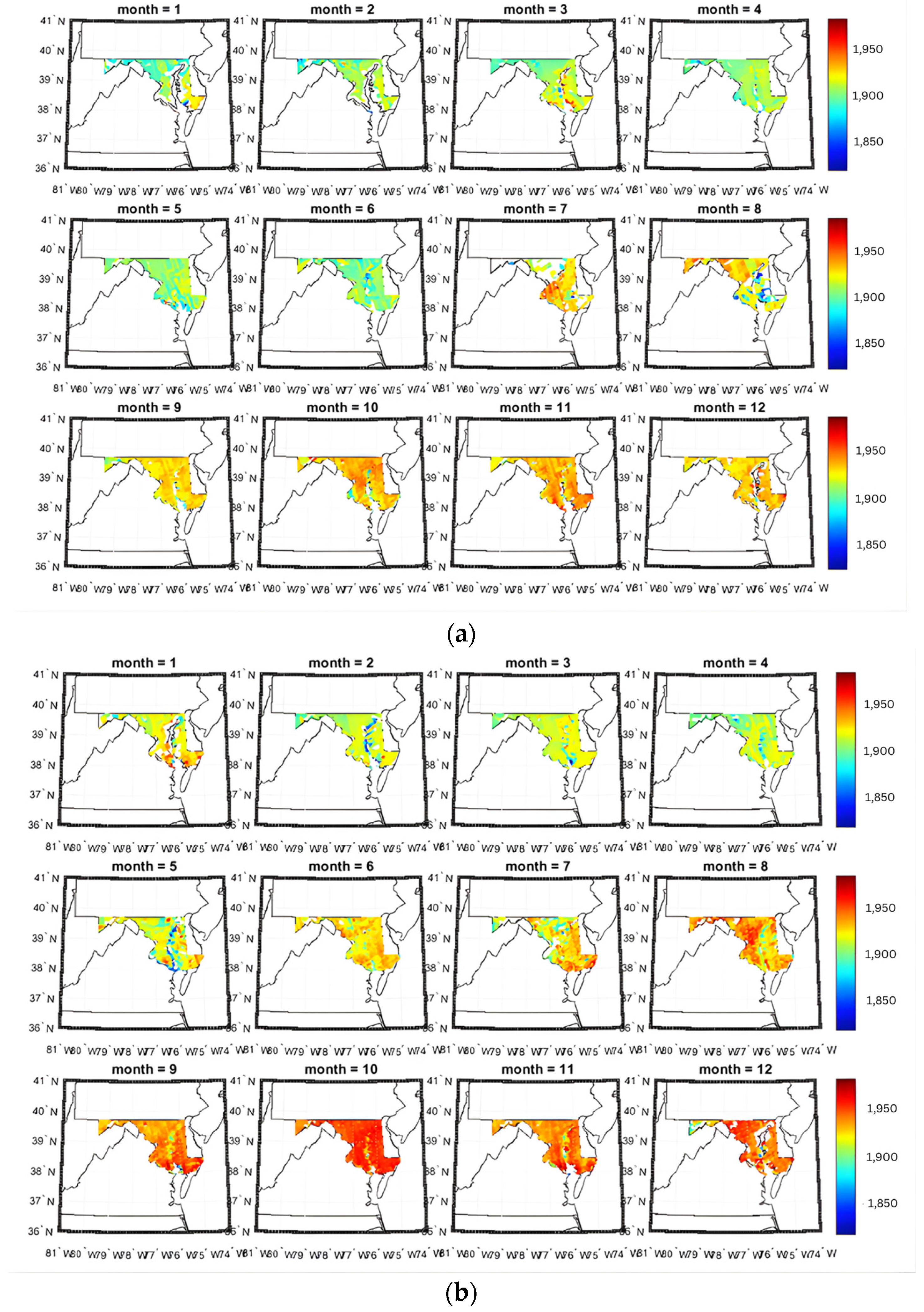
Correlation analysis further supported broad seasonal changes in methane concentrations due to temperature and time of year, reflecting larger-scale background variability. Satellite observations using TROPOMI trends(cf. Figure 19) corroborate the late-season elevation [44], displaying an increase in mean concentrations from October to December in the region of interest.
Figure 19.
2023–2024 monthly time series of mean CH4 concentrations in Maryland, USA, using the TROPOMI satellite for (a) 2023 and (b) 2024. Monthly trends corroborate ground measurements, displaying an increase in mean concentrations from October to December.
Ethane occasionally recorded negative values, likely reflecting instrument limitations at low ppb concentrations or low-signal bias near detection limits. In order to effectively identify whether a source is thermogenic using the Aeris Technologies instruments in ambient environments, it is recommended to maintain a water vapor mole fraction above 1% in the sample to preserve the integrity of ethane measurements, reduce the laser power when collecting, or humidify the sample line [45]. This still presents the risk of increased noise from increased water vapor sampling and was not implemented in this study.
Flight-to-flight variation of methane-altitude correlations revealed complex atmospheric stratification patterns, with both negative and positive altitude coefficients observed seasonally. Building on these results, we plan to extend this study by assessing nighttime methane sensitivity using thermometry-based satellite sensors. While the UAV platform and flight patterns were generally consistent, variability in flight path, altitude intervals, and meteorological conditions likely contributed to variability in concentration and correlation results. Hovering environments, such as over buildings, forests, and towers, also introduced small but noticeable changes to the vertical structure, though statistical comparisons indicated these differences remained within the range of natural atmospheric variability, likely reflecting localized turbulence and mechanical mixing near surface features rather than distinct micro-emission signatures. Despite these factors, the Aeris MIRA Strato showed a stable response, low drift, and sensitivity to environmental changes for boundary-layer characterization and ambient methane monitoring.
5. Conclusions
This study demonstrated the capability of the Aeris Technologies MIRA Strato analyzer for UAV-based ambient methane monitoring, capturing seasonal variability, diurnal patterns, and vertical structure within the atmospheric boundary-layer. These results underscore the value of UAV-based MWIR analyzers for ambient monitoring and highlight areas for improvement. Notably, the lack of comparative inlet measurements limited our ability to isolate rotor downwash effects, and detailed environmental characteristics such as building geometry, canopy density, or surrounding source distribution were not captured during profiling. These factors likely contributed to the observed variability across hovering environments. Future research should incorporate controlled inlet design evaluations, wind and turbulence analysis, and expanded site characterization to support more detailed correlation analysis. Overall, this work demonstrates not only the instrument’s robustness but also the capability of drone-deployed sensing to resolve fine-scale atmospheric variations without relying on direct plume quantification.
Author Contributions
Formal analysis, investigation, writing—original draft preparation, and visualization D.E. Drone deployment, N.N.K. Drone modification and visualization, R.K.S. Gas chamber calibration, R.K.S., P.S. and X.R. Project Administration, M.W. Writing—review, editing, and visualization, N.R.N. Writing—review and editing, A.F., J.R.V. and J.W. All authors have read and agreed to the published version of the manuscript.
Funding
This research was funded by the U.S Department of Energy (DOE) RENEW (grant no. DE-SC0024489), the National Aeronautics and Space Administration (NASA) Student Airborne Science Activation Program (grant no. 80NSSC21K0435), U.S. Department of Commerce, National Oceanic and Atmospheric Administration (NOAA), through the Educational Partnership Program (grant no. NA22SEC4810015), and the NOAA Cooperative Science Center for Atmospheric Sciences and Meteorology (NCAS-M).
Data Availability Statement
The data and visualization materials supporting the conclusions of this article will be made available by the authors on request.
Acknowledgments
The authors thank the National Geospatial-Intelligence Agency (NGA) and Howard University (HU) Cooperative Research and Development Agreement XHM0476CRFY 20001, Application of Remote Sensing for GEOINT, for providing technical assistance and instrument procurement.
Conflicts of Interest
The authors declare no conflicts of interest.
Disclaimer
The views expressed in this document do not necessarily reflect those of the National Geospatial-Intelligence Agency, the Department of War, or any other department or agency of the US Government.
References
- EPA Methane Emissions. Available online: www.epa.gov/ghgemissions/overview-greenhouse-gases (accessed on 30 May 2025).
- Predybaylo, E.; Lelieveld, J.; Pozzer, A.; Gromov, S.; Zimmermann, P.; Osipov, S.; Klingmüller, K.; Steil, B.; Stenchikov, G.; McCabe, M. Surface Temperature and Ozone Responses to the 2030 Global Methane Pledge. Clim. Change 2025, 178, 78. [Google Scholar] [CrossRef] [Scilit]
- Isaksen, I.; Berntsen, T.; Dalsøren, S.; Eleftheratos, K.; Orsolini, Y.; Rogneurd, B.; Stordal, F.; Søvde, O.A.; Zerefos, C.; Holmes, C. Atmospheric Ozone and Methane in a Changing Climate. Atmosphere 2014, 5, 518–535. [Google Scholar] [CrossRef] [Scilit]
- Rosentreter, J.A.; Alcott, L.; Maavara, T.; Sun, X.; Zhou, Y.; Planavsky, N.J.; Raymond, P.A. Revisiting the Global Methane Cycle Through Expert Opinion. Earths Future 2024, 12, e2023EF004234. [Google Scholar] [CrossRef] [Scilit]
- Ming, T.; De Richter, R.; Felzer, B.S.; Li, W. Jump in Tropospheric Methane Concentrations in 2020–2021 and Slowdown in 2022–2024: New Hypotheses on Causation. Atmosphere 2025, 16, 406. [Google Scholar] [CrossRef] [Scilit]
- Zhou, L.; Warner, J.; Nalli, N.R.; Wei, Z.; Oh, Y.; Bruhwiler, L.; Liu, X.; Divakarla, M.; Pryor, K.; Kalluri, S.; et al. Spatiotemporal Variability of Global Atmospheric Methane Observed from Two Decades of Satellite Hyperspectral Infrared Sounders. Remote Sens. 2023, 15, 2992. [Google Scholar] [CrossRef] [Scilit]
- Saunois, M.; Martinez, A.; Poulter, B.; Zhang, Z.; Raymond, P.A.; Regnier, P.; Canadell, J.G.; Jackson, R.B.; Patra, P.K.; Bousquet, P.; et al. Global Methane Budget 2000–2020. Earth Syst. Sci. Data 2025, 17, 1873–1958. [Google Scholar] [CrossRef] [Scilit]
- United Nations Environmental Programme/Climate and Clean Air Coalition. Global Methane Assessment: 2030 Baseline Report; United Nations Environment Programme: Nairobi, Kenya, 2022. [Google Scholar]
- Stolper, D.A.; Martini, A.M.; Clog, M.; Douglas, P.M.; Shusta, S.S.; Valentine, D.L.; Sessions, A.L.; Eiler, J.M. Distinguishing and Understanding Thermogenic and Biogenic Sources of Methane Using Multiply Substituted Isotopologues. Geochim. Cosmochim. Acta 2015, 161, 219–247. [Google Scholar] [CrossRef] [Scilit]
- Wuebbles, D. Atmospheric Methane and Global Change. Earth-Sci. Rev. 2002, 57, 177–210. [Google Scholar] [CrossRef] [Scilit]
- Stolper, D.A.; Lawson, M.; Davis, C.L.; Ferreira, A.A.; Neto, E.V.S.; Ellis, G.S.; Lewan, M.D.; Martini, A.M.; Tang, Y.; Schoell, M.; et al. Formation Temperatures of Thermogenic and Biogenic Methane. Science 2014, 344, 1500–1503. [Google Scholar] [CrossRef] [Scilit] [PubMed]
- Booth, J.; Rowe, M.; Fischer, K. Offshore Gas Hydrate Sample Database with an Overview and Preliminary Analysis; U.S. Geological Survey Open-File Report; USGS Woods Hole Science Center: Woods Hole, MA, USA, 1996.
- Sherwood, O.A.; Travers, P.D.; Dolan, M.P. Compound-Specific Stable Isotope Analysis of Natural and Produced Hydrocarbon Gases Surrounding Oil and Gas Operations. In Comprehensive Analytical Chemistry; Elsevier: Amsterdam, The Netherlands, 2013; Volume 61, pp. 347–372. ISBN 978-0-444-62623-3. [Google Scholar]
- Kirschke, S.; Bousquet, P.; Ciais, P.; Saunois, M.; Canadell, J.G.; Dlugokencky, E.J.; Bergamaschi, P.; Bergmann, D.; Blake, D.R.; Bruhwiler, L.; et al. Three Decades of Global Methane Sources and Sinks. Nat. Geosci. 2013, 6, 813–823. [Google Scholar] [CrossRef] [Scilit]
- Li, Q.; Meidan, D.; Hess, P.; Añel, J.A.; Cuevas, C.A.; Doney, S.; Fernandez, R.P.; Van Herpen, M.; Höglund-Isaksson, L.; Johnson, M.S.; et al. Global Environmental Implications of Atmospheric Methane Removal through Chlorine-Mediated Chemistry-Climate Interactions. Nat. Commun. 2023, 14, 4045. [Google Scholar] [CrossRef] [Scilit]
- Gorham, K.A.; Abernethy, S.; Jones, T.R.; Hess, P.; Mahowald, N.M.; Meidan, D.; Johnson, M.S.; Van Herpen, M.M.J.W.; Xu, Y.; Saiz-Lopez, A.; et al. Opinion: A Research Roadmap for Exploring Atmospheric Methane Removal via Iron Salt Aerosol. Atmos. Chem. Phys. 2024, 24, 5659–5670. [Google Scholar] [CrossRef] [Scilit]
- Li, W.; Liu, Y.; Yao, X.; Ming, T.; De Richter, R. Removal of Atmospheric Methane by Increasing Hydroxyl Radicals via a Water Vapor Enhancement Strategy. Atmosphere 2024, 15, 1046. [Google Scholar] [CrossRef] [Scilit]
- Heimann, I.; Griffiths, P.T.; Warwick, N.J.; Abraham, N.L.; Archibald, A.T.; Pyle, J.A. Methane Emissions in a Chemistry-Climate Model: Feedbacks and Climate Response. J. Adv. Model. Earth Syst. 2020, 12, e2019MS002019. [Google Scholar] [CrossRef] [Scilit]
- Stevenson, D.S.; Zhao, A.; Naik, V.; O’Connor, F.M.; Tilmes, S.; Zeng, G.; Murray, L.T.; Collins, W.J.; Griffiths, P.T.; Shim, S.; et al. Trends in Global Tropospheric Hydroxyl Radical and Methane Lifetime since 1850 from AerChemMIP. Atmospheric Chem. Phys. 2020, 20, 12905–12920. [Google Scholar] [CrossRef] [Scilit]
- He, L.; Groom, J.D.; Wilson, E.H.; Fernandez, J.; Konopka, M.C.; Beck, D.A.C.; Lidstrom, M.E. A Methanotrophic Bacterium to Enable Methane Removal for Climate Mitigation. Proc. Natl. Acad. Sci. USA 2023, 120, e2310046120. [Google Scholar] [CrossRef] [Scilit] [PubMed]
- Umweltbundesamt. Technical Approaches to Removing Methane from the Atmosphere (Methane Removal): Fact Check and Discussion; Umweltbundesamt: Dessau-Roßlau, Germany, 2024. [Google Scholar]
- Committee on Anthropogenic Methane Emissions in the United States: Improving Measurement, Monitoring, Presentation of Results, and Development of Inventories; Board on Atmospheric Sciences and Climate; Board on Agriculture and Natural Resources; Board on Earth Sciences and Resources; Board on Energy and Environmental Systems; Board on Environmental Studies and Toxicology; Division on Earth and Life Studies; National Academies of Sciences, Engineering, and Medicine. Improving Characterization of Anthropogenic Methane Emissions in the United States; National Academies Press: Washington, DC, USA, 2018; p. 24987. ISBN 978-0-309-47050-6. [Google Scholar]
- Fosco, D.; De Molfetta, M.; Renzulli, P.A.; Notarnicola, B.; Dimauro, G.; Astuto, F.; Spizzirri, U.G. Drone-Based Methane Emission Estimation at Waste, Livestock and Energy Facilities: Experimental Tests in Italy and Challenges of Wind–Concentration Integration with Open-Path Sensors. J. Environ. Manag. 2026, 398, 128290. [Google Scholar] [CrossRef] [Scilit] [PubMed]
- Shaw, J.T.; Shah, A.; Yong, H.; Allen, G. Methods for Quantifying Methane Emissions Using Unmanned Aerial Vehicles: A Review. Philos. Trans. R. Soc. Math. Phys. Eng. Sci. 2021, 379, 20200450. [Google Scholar] [CrossRef] [Scilit] [PubMed]
- Watts, A.C.; Ambrosia, V.G.; Hinkley, E.A. Unmanned Aircraft Systems in Remote Sensing and Scientific Research: Classification and Considerations of Use. Remote Sens. 2012, 4, 1671–1692. [Google Scholar] [CrossRef] [Scilit]
- Yang, S.; Talbot, R.W.; Frish, M.B.; Golston, L.M.; Aubut, N.F.; Zondlo, M.A.; Gretencord, C.; McSpiritt, J. Natural Gas Fugitive Leak Detection Using an Unmanned Aerial Vehicle: Measurement System Description and Mass Balance Approach. Atmosphere 2018, 9, 383. [Google Scholar] [CrossRef] [Scilit]
- Dooley, J.F.; Minschwaner, K.; Dubey, M.K.; El Abbadi, S.H.; Sherwin, E.D.; Meyer, A.G.; Follansbee, E.; Lee, J.E. A New Aerial Approach for Quantifying and Attributing Methane Emissions: Implementation and Validation. Atmos. Meas. Tech. 2024, 17, 5091–5111. [Google Scholar] [CrossRef] [Scilit]
- Hollenbeck, D.; Nunez, G.; Christensen, L.E.; Chen, Y. Wind Measurement and Estimation with Small Unmanned Aerial Systems (sUAS) Using On-Board Mini Ultrasonic Anemometers. In Proceedings of the 2018 International Conference on Unmanned Aircraft Systems (ICUAS), Dallas, TX, USA, 12–15 June 2018; IEEE: Piscataway, NJ, USA, 2018; pp. 285–292. [Google Scholar]
- McKinney, K.A.; Wang, D.; Ye, J.; De Fouchier, J.-B.; Guimarães, P.C.; Batista, C.E.; Souza, R.A.F.; Alves, E.G.; Gu, D.; Guenther, A.B.; et al. A Sampler for Atmospheric Volatile Organic Compounds by Copter Unmanned Aerial Vehicles. Atmos. Meas. Tech. 2019, 12, 3123–3135. [Google Scholar] [CrossRef] [Scilit]
- Villa, T.; Gonzalez, F.; Miljievic, B.; Ristovski, Z.; Morawska, L. An Overview of Small Unmanned Aerial Vehicles for Air Quality Measurements: Present Applications and Future Prospectives. Sensors 2016, 16, 1072. [Google Scholar] [CrossRef] [Scilit] [PubMed]
- Burgués, J.; Marco, S. Environmental Chemical Sensing Using Small Drones: A Review. Sci. Total Environ. 2020, 748, 141172. [Google Scholar] [CrossRef] [Scilit] [PubMed]
- Acharya, B.S.; Bhandari, M.; Bandini, F.; Pizarro, A.; Perks, M.; Joshi, D.R.; Wang, S.; Dogwiler, T.; Ray, R.L.; Kharel, G.; et al. Unmanned Aerial Vehicles in Hydrology and Water Management: Applications, Challenges, and Perspectives. Water Resour. Res. 2021, 57, e2021WR029925. [Google Scholar] [CrossRef] [Scilit]
- Jońca, J.; Pawnuk, M.; Bezyk, Y.; Arsen, A.; Sówka, I. Drone-Assisted Monitoring of Atmospheric Pollution—A Comprehensive Review. Sustainability 2022, 14, 11516. [Google Scholar] [CrossRef] [Scilit]
- Kaliszewski, M.; Włodarski, M.; Młyńczak, J.; Jankiewicz, B.; Auer, L.; Bartosewicz, B.; Liszewska, M.; Budner, B.; Szala, M.; Schneider, B.; et al. The Multi-Gas Sensor for Remote UAV and UGV Missions—Development and Tests. Sensors 2021, 21, 7608. [Google Scholar] [CrossRef] [Scilit] [PubMed]
- Madokoro, H.; Kiguchi, O.; Nagayoshi, T.; Chiba, T.; Inoue, M.; Chiyonobu, S.; Nix, S.; Woo, H.; Sato, K. Development of Drone-Mounted Multiple Sensing System with Advanced Mobility for In Situ Atmospheric Measurement: A Case Study Focusing on PM2.5 Local Distribution. Sensors 2021, 21, 4881. [Google Scholar] [CrossRef] [Scilit]
- Aeris Technologies. MIRA Strato LDS: UAV/Drone Natural Gas Leak Detection System w/GPS; Aeris Technologies: Hayward, CA, USA, 2021; p. 2. Available online: https://aerissensors.com/wp-content/uploads/2021/12/MIRA-Strato-LDS_Drone_211209.pdf (accessed on 7 May 2025).
- Paschotta, R. Spectroscopy. RP Photonics Encycl. Available online: https://www.rp-photonics.com/spectroscopy.html (accessed on 8 April 2025).
- Paschotta, R. Multipass Gas Cells. RP Photonics Encycl. Available online: https://www.rp-photonics.com/multipass_gas_cells.html (accessed on 23 April 2025).
- Picarro, Inc. G2401 Gas Concentration Analyzer. Available online: https://www.picarro.com/environmental/products/g2401_gas_concentration_analyzer (accessed on 30 April 2025).
- Wheeler, M.D.; Newman, S.M.; Orr-Ewing, A.J.; Ashfold, M.N.R. Cavity Ring-down Spectroscopy. J. Chem. Soc. Faraday Trans. 1998, 94, 337–351. [Google Scholar] [CrossRef] [Scilit]
- Borhan, M.S.; Khanaum, M.M. Sensors and Methods for Measuring Greenhouse Gas Emissions from Different Components of Livestock Production Facilities. J. Geosci. Environ. Prot. 2022, 10, 242–272. [Google Scholar] [CrossRef]
- Bauer, P.; Nagy, M. Flight-Data-Based High-Fidelity System Identification of DJI M600 Pro Hexacopter. Aerospace 2024, 11, 79. [Google Scholar] [CrossRef] [Scilit]
- DJI Matrice 600 Pro User Manual PDF. Available online: https://dl.djicdn.com/downloads/m600%20pro/20180417/Matrice_600_Pro_User_Manual_v1.0_EN.pdf (accessed on 7 June 2025).
- Lampert, A.; Pätzold, F.; Asmussen, M.O.; Lobitz, L.; Krüger, T.; Rausch, T.; Sachs, T.; Wille, C.; Sotomayor Zakharov, D.; Gaus, D.; et al. Studying Boundary Layer Methane Isotopy and Vertical Mixing Processes at a Rewetted Peatland Site Using an Unmanned Aircraft System. Atmos. Meas. Tech. 2020, 13, 1937–1952. [Google Scholar] [CrossRef] [Scilit]
- Commane, R.; Hallward-Driemeier, A.; Murray, L.T. Intercomparison of Commercial Analyzers for Atmospheric Ethane and Methane Observations. Atmos. Meas. Tech. 2023, 16, 1431–1441. [Google Scholar] [CrossRef] [Scilit]
- Levrault, C.M.; Difford, G.F.; Steinheim, G.; Groot Koerkamp, P.W.G.; Ogink, N.W.M. Validation of the Methane Production Measurement Accuracy and Ranking Capacity of Portable Accumulation Chambers for Use with Small Ruminants. Biosyst. Eng. 2023, 236, 201–211. [Google Scholar] [CrossRef] [Scilit]

Disclaimer/Publisher’s Note: The statements, opinions and data contained in all publications are solely those of the individual author(s) and contributor(s) and not of MDPI and/or the editor(s). MDPI and/or the editor(s) disclaim responsibility for any injury to people or property resulting from any ideas, methods, instructions or products referred to in the content. |
© 2026 by the authors. Licensee MDPI, Basel, Switzerland. This article is an open access article distributed under the terms and conditions of the Creative Commons Attribution (CC BY) license.