Evaluation of a LUE Model and Various Water Scalars Based on Eddy Covariance Data from 13 Forest Sites Across Europe

Highlights

What are the main findings?

• sCASE produces highly accurate GPP estimates for a variety of forest ecosystems. The developmental state of deciduous species should not be neglected by productivity models.
• Water balance-based water scalars are optimum for water-limited sites but a VPD-based scalar performed better in sites with ample water. MODIS-derived water indices had an overall good performance as water scalars.

What are the implications of the main findings?

• sCASE can be used for the estimation of the GPP of different forest ecosystems. The developmental scalar should be incorporated in productivity models.
• Water scalars should further evolve in order to better represent water status effects on productivity. Remote sensing-derived water indices can be used as water scalars in large-scale applications with relatively low bias.

Abstract

Light use efficiency (LUE) models are widely used to estimate gross primary productivity (GPP) because they provide strong accuracy while maintaining low complexity. The aim of this study is (a) to evaluate the performance of a LUE model (sCASE) and (b) to compare the performance of several alternative water scalars. The analyses are done using GPP measurements from thirteen eddy covariance sites across Europe, corresponding to different forest types. Daily GPP estimates produced by sCASE were highly accurate for most sites (average R² = 0.750 and average RMSE = 2.317 g C m⁻² d⁻¹), matching the performance of other widely used LUE models in the literature. All three scalars were essential for maintaining model accuracy, although their relative importance varied among sites. The developmental scalar, which is not incorporated in most productivity models, was particularly important for accurately estimating GPP in deciduous species. Among the ten water scalars tested, those based on simple water balance calculations performed best in water-limited sites, whereas the VPD-based scalar performed better in sites without water limitation. The EF (evaporative fraction) scalar showed high accuracy at some sites across both water status categories but very low accuracy at others. For large-scale applications, water scalars based on MODIS indices offer the advantage of global coverage, which can outweigh their lower accuracy relative to other scalars.

1. Introduction

The light use efficiency (LUE) concept describes an empirical relationship between produced biomass and available radiation [1,2], and it is also used for the estimation of gross primary productivity (GPP), linking radiation to CO₂ sequestration rather than biomass production [3]. Productivity models based on this concept, commonly referred to as LUE models, are linked to remote sensing, as they have relied on satellite-derived data since their early development [4,5]. Following the LUE framework, these models estimate GPP as the product of Absorbed Photosynthetically Active Radiation (APAR) and the efficiency (LUE) with which the absorbed radiation is converted into biomolecules through photosynthesis:

$$\mathrm{G}\mathrm{P}\mathrm{P}=\mathrm{A}\mathrm{P}\mathrm{A}\mathrm{R}\mathrm{\ast }\mathrm{L}\mathrm{U}\mathrm{E}$$

(1)

Although LUE models in the literature are based on the same underlying concept, they can differ substantially in their structure, parameterization, and input datasets [6]. Both APAR and LUE can be estimated using various methods, which leads to different GPP values and, consequently, different model accuracies [7]. LUE is a dynamic parameter that varies across space and time according to species, vegetation age, phenological state [8,9], and meteorological conditions [10,11]. Typically, LUE models assign a maximum LUE value to each vegetation type [12], which is then downregulated using equations (scalars) that represent the effects of limiting factors on photosynthesis [13,14]. The most commonly used scalars account for temperature and water availability [15], while some studies have also incorporated scalars for the developmental stage [16], CO₂ fertilization [17], and diffuse radiation [18]. However, the mechanisms through which these factors regulate LUE remain uncertain, and there is no consensus on how they should be incorporated into models [19]. This lack of agreement is particularly evident for water limitation, where differences exist not only in the equations used to represent its effect on productivity but also in the choice of water indicator on which these equations are based [20,21]. Following the Soil Plant Atmosphere Continuum (SPAC) framework [22], water scalars can be grouped into three categories according to the level at which they detect water limitation: (a) atmospheric, (b) soil, and (c) vegetation [15,21]. Vapor Pressure Deficit (VPD) is the most commonly used atmospheric indicator, while Soil Water Content (SWC) is the most widely used soil-based indicator. The vegetation-based category includes indicators such as the evaporative fraction [23] and shortwave reflection vegetation indices [24].

On the other hand, temperature scalars are less diverse, largely because the effects of temperature on photosynthesis are well understood. Temperature regulates the activity of key enzymes, with both high and low temperatures suppressing photosynthesis [25]. The photosynthetic rate increases with temperature until it reaches an optimum (T_opt), beyond which it declines [26]. In addition to this optimum, two critical thresholds exist: the maximum (T_max) and minimum (T_min) temperatures, above and below which (respectively) photosynthesis is completely inhibited. Temperature scalars incorporate this temperature/photosynthesis relationship to adjust LUE under varying thermal conditions, using one or more of these critical temperatures [4,24]. Most LUE models employ a bell-shaped curve defined by all three temperature thresholds.

GPP is a key component of the carbon cycle [27] and plays a crucial role in mitigating rising atmospheric CO₂ concentrations and the resulting climate change [28]. Although global GPP has increased in recent decades [29] due to warmer temperatures and elevated CO₂, extreme heatwaves and droughts have caused substantial reductions in productivity [30,31]. Ecosystems characterized by high temperatures and limited rainfall are among the least productive and exhibit a declining trend over time [32,33,34]. The importance of heat and drought stress is expected to intensify in the coming years [35], increasingly affecting even highly productive regions such as tropical rainforests that were previously unaffected [36,37]. Consequently, many researchers have expressed concerns about the future role of terrestrial vegetation in the carbon cycle, as climate-induced stresses threaten forest functioning and health [38,39,40].

In order to fully understand how GPP responds to climate change and its future role in the carbon cycle, it is essential to accurately estimate productivity at large to global scales. Among the various factors influencing the performance of LUE models, the accurate representation of water availability effects on productivity is one of the most critical, yet it remains insufficiently resolved [20]. Uncertainties in water scalars arise from variability in the underlying indicators, differences in scalar formulations, and limitations in input data quality [15]. This study focuses on two main objectives. Firstly, it evaluates the accuracy of a LUE model (sCASE) [41] using measurements from thirteen eddy covariance towers across Europe, corresponding to forest ecosystems with contrasting water status conditions. Secondly, using this model framework, it assesses the ability of several water scalars, each based on different indicators, to accurately capture the effects of water availability on GPP.

2. Materials and Methods

2.1. Species and Study Sites

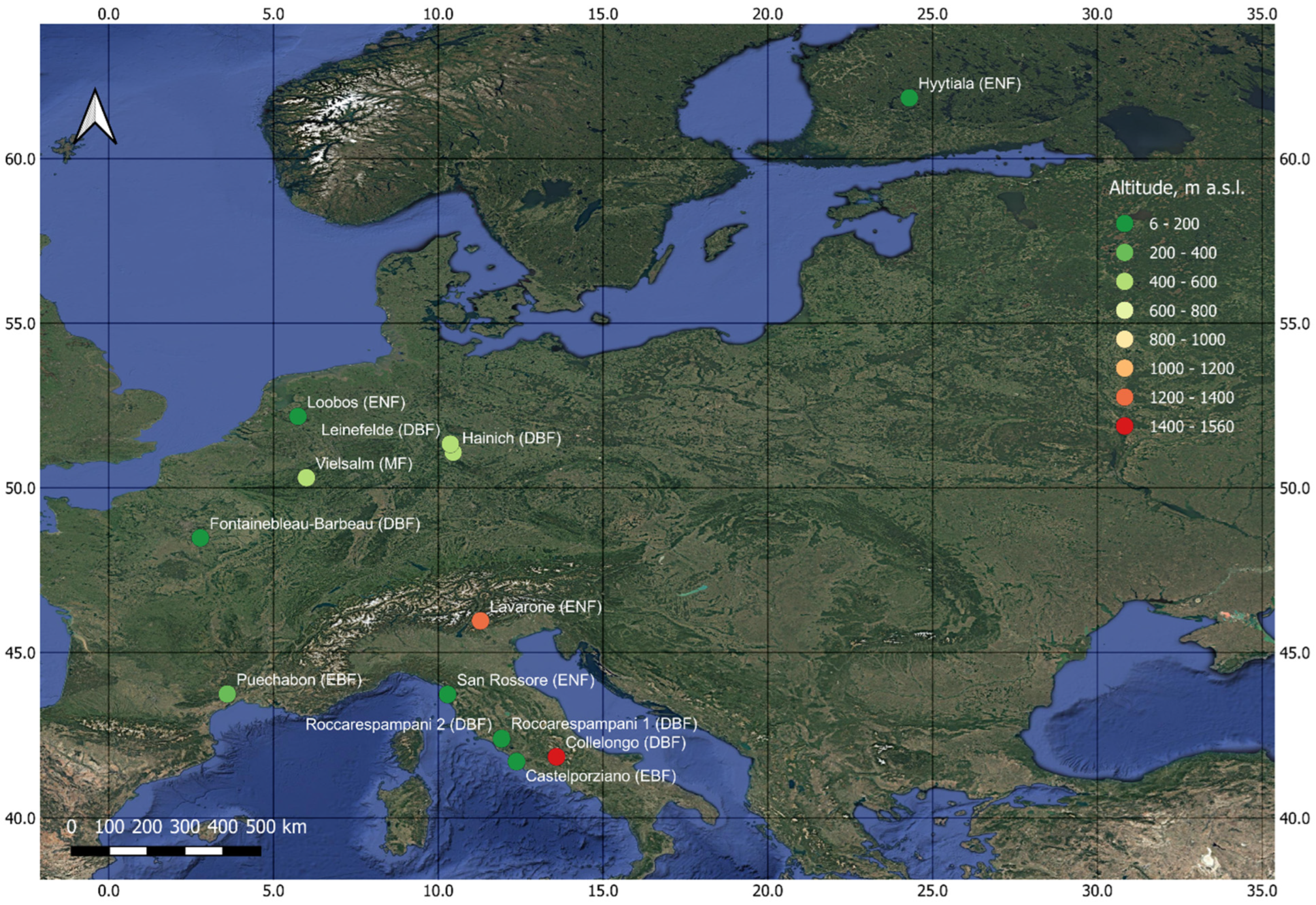
The present study is conducted across thirteen eddy covariance sites representing a range of forest ecosystems (evergreen and deciduous) that differ substantially in their climatological regimes. All sites feature dense canopies, particularly in the area surrounding each tower, with the dominant species accounting for more than 80% of the overstory vegetation. Site-specific information, including coordinates, dominant species, and analysis period, is provided in

Table 1. The thirteen eddy covariance sites of this study. The vegetation type of each site based on the International Geosphere-Biosphere Programme (IGBP) is provided inside the parentheses next to the site name: MF = mixed forest, ENF = evergreen needleleaf forest, DBF = deciduous broadleaf forest and EBF = evergreen broadleaf forest.

Site Name	Elevation, m a.s.l.	Latitude	Longitude	Dominant Species	Study Period	Country
Vielsalm (MF)	493	50.3049°N	5.9981°E	Pseudotsuga menziesii, Fagus sylvatica	2001–2014	Belgium
Hyytiälä (ENF)	181	61.8474°N	24.2947°E	Pinus sylvestris	2001–2014	Finland
Lavarone (ENF)	1353	45.9562°N	11.2813°E	Abies alba, Picea abies	2003–2014	Italy
Loobos (ENF)	25	52.1665°N	5.7436°E	Pinus sylvestris	2001–2014	Netherlands
Hainich (DBF)	430	51.0792°N	10.4521°E	Fagus sylvatica, Fraxinus excelsior	2001–2012	Germany
Leinefelde (DBF)	451	51.3282°N	10.3678°E	Fagus sylvatica	2002–2006 and 2010–2012	Germany
Fontainebleau-Barbeau (DBF)	103	48.4763°N	2.7801°E	Quercus petrea	2005–2014	France
Collelongo (DBF)	1560	41.8493°N	13.5881°E	Fagus sylvatica	2001–2014	Italy
Roccarespampani 1 (DBF)	235	42.4081°N	11.9300°E	Quercus cerris	2001–2008	Italy
Roccarespampani 2 (DBF)	160	42.3902°N	11.9209°E	Quercus cerris	2002–2008 and 2010–2012	Italy
San Rossore (ENF)	6	43.7278°N	10.2844°E	Pinus pinaster, Pinus pinea	2001–2012	Italy
Puéchabon (EBF)	270	43.7413°N	3.5957°E	Quercus ilex	2001–2014	France
Castelporziano (EBF)	68	41.7052°N	12.3761°E	Quercus ilex	2001–2008	Italy

and Figure 1.

2.2. Satellite Data

For this study, two MODIS products were used: MOD09A1 and MOD17A2. MOD09A1 is an eight-day composite product that provides surface reflectance values for the first seven MODIS bands at a spatial resolution of 500 m in sinusoidal projection. These data were used to calculate six vegetation and water indices, as described below. Images of poor quality (e.g., snow, cloud contamination) were excluded based on the product’s quality bands. The MOD17A2 product provides GPP estimates generated by the MODIS productivity model [42] at eight-day intervals and a spatial resolution of 500 m. This productivity model is a LUE-based approach that produces global GPP estimates and is widely used as a reference dataset.

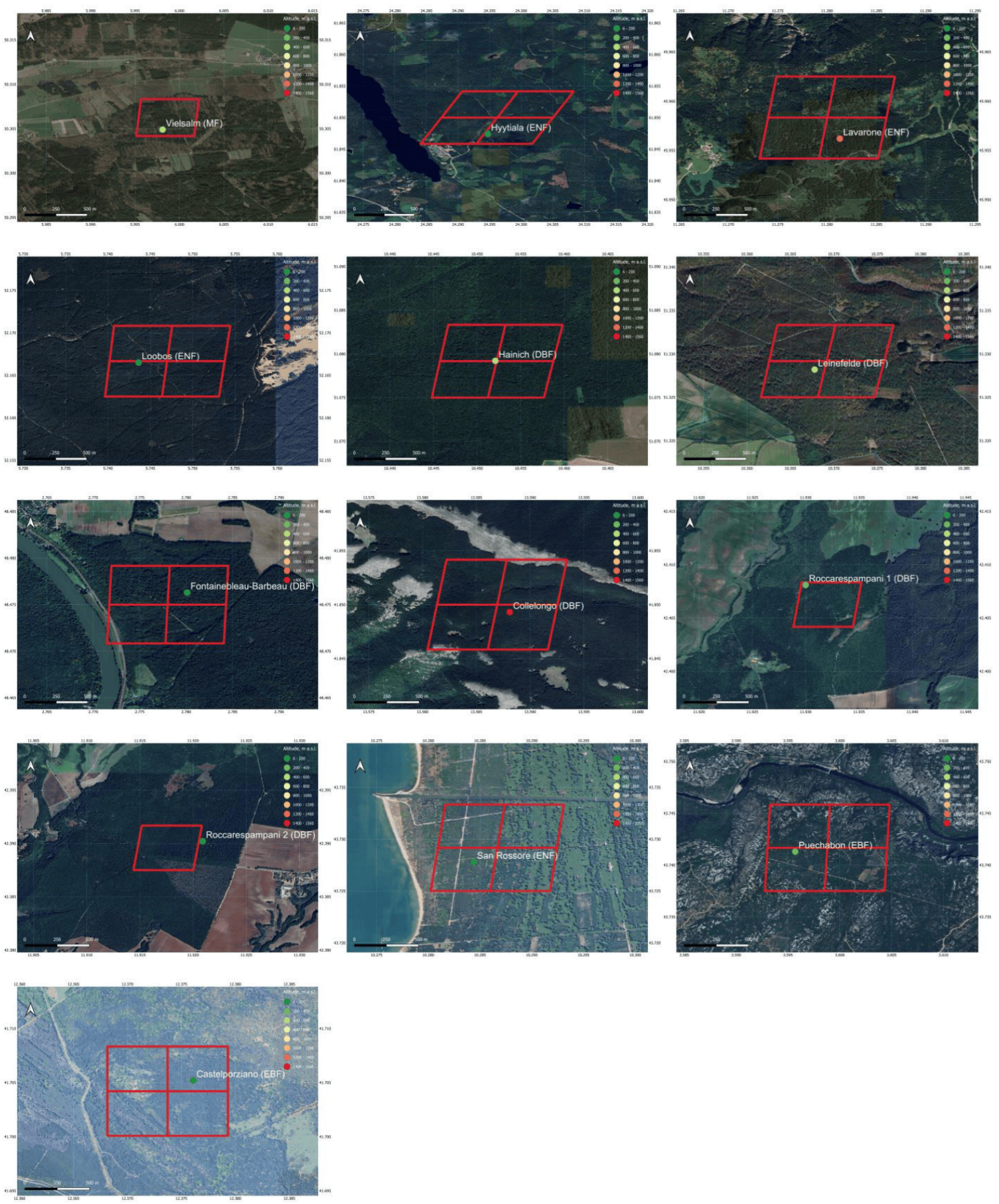
Both MODIS products were obtained through NASA’s Terrestrial Ecology Subsetting & Visualization Services (TESViS) portal (https://modis.ornl.gov/ accessed on 25 January 2021), which provides MODIS datasets for predefined or user-specified locations in CSV format. For each site, four MODIS pixels (500 m) surrounding the eddy covariance tower were selected (covering approximately 1 km²) based on visual assessment of the area (Appendix A). The 1 km² area is considered adequate for the eddy covariance towers of this study, which are of medium height and relatively close to the canopy. Studies have shown that such towers have a footprint area of approximately 1 km² [43,44]. In three sites, Vielsalm, Roccarespampani 1 and Roccarespampani 2, only one pixel was used due to the small extent of the forest relative to the tower position (Figure A1). The selected pixels are considered homogenous in terms of functional vegetation type, and for each site, the average index (or GPP) value of the selected pixels was used. NDVI and RDVI indices were corrected for anomalies using an alternative implementation of the BISE algorithm (Best Index Slope Extraction [45]) and subsequently smoothed using a 5-point adjacent-averaging filter. The four water indices were left unmodified, as they reflect dynamic conditions in which rapid fluctuations are not necessarily erroneous. However, to avoid inconsistencies in the time series, water index values corresponding to dates on which the NDVI was corrected were excluded. Daily values for all indices were generated through simple linear interpolation.

2.3. Eddy Covariance Data

The eddy covariance data for the thirteen sites were obtained from the FLUXNET2015 dataset (https://fluxnet.fluxdata.org/ accessed on 13 May 2020), which includes measurements from all towers in the FLUXNET network from their installation through 2014. All the data have been processed using standardized methods and are provided at half-hourly, daily, weekly, monthly and yearly timesteps. In addition to GPP, the FLUXNET2015 dataset includes a wide range of energy flux and meteorological variables. For each parameter, multiple versions are available, reflecting differences in estimation methods, data corrections, and gap-filling algorithms [46]. The specific FLUXNET2015 variables used in this study are listed in

Table 2. The various parameters of the eddy covariance towers used in this study. The data are from the FLUXNET2015 dataset. The timestep refers to the source data timestep (as FLUXNET2015 provides data in different timesteps).

Parameter	Timestep	Units
Temperature	Half-hour	°C
Precipitation	Daily	mm
SW potential	Half-hour	W m−2
SW incoming	Half-hour	W m−2
PPFD	Half-hour	μmol photons m−2 s−1
VPD	Daily	hPa
Wind speed	Daily	m s−2
GPP	Daily	g C m−2 d−1
SWC	Daily	%
Latent heat flux	Daily	W m−2
Sensible heat flux	Daily	W m−2

.

PAR values were derived from incoming shortwave (SW) radiation by multiplying SW with a site-specific factor that depends on latitude [47], because the PAR data in the FLUXNET2015 dataset have missing values even after the gap filling. Half-hourly SW radiation (W m⁻²) from FLUXNET2015 was converted to half-hourly PAR (μmol m⁻² s⁻¹) using this factor, and subsequently aggregated to daily PAR (mol m⁻² d⁻¹). The site-specific factor was determined from the linear relationship between incoming SW radiation and Photosynthetic Photon Flux Density (PPFD) in the half-hourly dataset. Daily temperature values were also calculated from the half-hourly data in order to obtain minimum and maximum daily temperatures, which are not provided in the FLUXNET2015 daily product. Average daily temperatures were likewise computed from the half-hourly data and matched those of the daily dataset. All other variables used in this study were taken directly from the daily FLUXNET2015 dataset.

Among the various GPP variations available in FLUXNET2015, we selected the version derived using the nighttime partitioning method [48], based on a reference Net Ecosystem Exchange (NEE) dataset with a Variable Ustar Threshold (VUT). This reference NEE was chosen according to the Model Efficiency criterion applied across the different NEE versions in FLUXNET2015 [49].

2.4. sCASE Model

sCASE [41,50] is a LUE model that uses MODIS/Terra (MOD09A1) surface reflectance data and meteorological inputs to calculate daily GPP according to the following equation:

$$\mathrm{G}\mathrm{P}\mathrm{P}=\mathrm{P}\mathrm{A}\mathrm{R}\mathrm{\ast }\mathrm{f}\mathrm{A}\mathrm{P}\mathrm{A}\mathrm{R}\mathrm{\ast }{\mathrm{L}\mathrm{U}\mathrm{E}}_{\mathrm{m}\mathrm{a}\mathrm{x}}\mathrm{\ast }{\mathrm{D}}_{\mathrm{s}\mathrm{c}\mathrm{a}\mathrm{l}\mathrm{a}\mathrm{r}}\mathrm{\ast }{\mathrm{T}}_{\mathrm{s}\mathrm{c}\mathrm{a}\mathrm{l}\mathrm{a}\mathrm{r}}\mathrm{\ast }{\mathrm{W}}_{\mathrm{s}\mathrm{c}\mathrm{a}\mathrm{l}\mathrm{a}\mathrm{r}}$$

(2)

where PAR is the Photosynthetically Active Radiation, fAPAR is the fraction of Absorbed Photosynthetically Active Radiation, and LUE_max is the maximum light use efficiency assigned to each species or vegetation type. The three scalars, D_scalar, T_scalar and W_scalar, downregulate LUE to account for the effects of the developmental stage, temperature and water status, respectively.

PAR, T_scalar and W_scalar are derived from meteorological data (with PAR directly measured), whereas fAPAR and D_scalar are estimated from the NDVI (Normalized Difference Vegetation Index) [51] and RDVI (Renormalized Difference Vegetation Index) [52], respectively, both calculated from the MOD09A1 product. fAPAR is computed from the NDVI in two steps: firstly, the NDVI is used to estimate the Leaf Area Index (LAI), using the empirical relationship in Equation (3), and the LAI is then used to calculate fAPAR from Equation (4) [13], where k_d is the canopy light extinction coefficient (set to 0.65 for all sites).

$$\mathrm{L}\mathrm{A}\mathrm{I}=0.035\mathrm{\ast }{\mathrm{e}}^{{\displaystyle \frac{\mathrm{N}\mathrm{D}\mathrm{V}\mathrm{I}}{0.17}}}$$

(3)

$$\mathrm{f}\mathrm{A}\mathrm{P}\mathrm{A}\mathrm{R}=\left(1-{\mathrm{e}}^{-{\mathrm{k}}_{\mathrm{d}}\mathrm{\ast }\mathrm{L}\mathrm{A}\mathrm{I}}\right)\mathrm{\ast }0.95$$

(4)

The developmental scalar (D_scalar) is calculated from the RDVI using two formulations, one for deciduous sites (Equation (5)) and one for evergreen and mixed sites (Equation (6)).

$${\mathrm{D}}_{\mathrm{s}\mathrm{c}\mathrm{a}\mathrm{l}\mathrm{a}\mathrm{r}}={\displaystyle \frac{1}{1+100\mathrm{\ast }{\mathrm{e}}^{-12\mathrm{\ast }\frac{\mathrm{R}\mathrm{D}\mathrm{V}\mathrm{I}-0.15}{0.55}}}}$$

(5)

$${\mathrm{D}}_{\mathrm{s}\mathrm{c}\mathrm{a}\mathrm{l}\mathrm{a}\mathrm{r}}={\displaystyle \frac{1}{1+150\mathrm{\ast }{\mathrm{e}}^{-15\mathrm{\ast }\frac{\mathrm{R}\mathrm{D}\mathrm{V}\mathrm{I}}{0.6}}}}$$

(6)

The temperature scalar is based on a bell-shaped response curve, utilizing the three critical temperatures (T_opt, T_max, T_min), and is calculated using Equation (7), where T_day is the mean daytime temperature.

$${\mathrm{T}}_{\mathrm{s}\mathrm{c}\mathrm{a}\mathrm{l}\mathrm{a}\mathrm{r}}={\displaystyle \frac{\left({\mathrm{T}}_{\mathrm{d}\mathrm{a}\mathrm{y}}-{\mathrm{T}}_{\mathrm{m}\mathrm{i}\mathrm{n}}\right)\mathrm{\ast }\left({\mathrm{T}}_{\mathrm{d}\mathrm{a}\mathrm{y}}-\right.\left.{\mathrm{T}}_{\mathrm{m}\mathrm{a}\mathrm{x}}\right)}{\left[\left({\mathrm{T}}_{\mathrm{d}\mathrm{a}\mathrm{y}}-\left.{\mathrm{T}}_{\mathrm{m}\mathrm{i}\mathrm{n}}\right)\right.\mathrm{\ast }\left({\mathrm{T}}_{\mathrm{d}\mathrm{a}\mathrm{y}}-\left.{\mathrm{T}}_{\mathrm{m}\mathrm{a}\mathrm{x}}\right)\right.\right]-{\left({\mathrm{T}}_{\mathrm{d}\mathrm{a}\mathrm{y}}\right.\left.{-\mathrm{T}}_{\mathrm{o}\mathrm{p}\mathrm{t}}\right)}^2}}$$

(7)

Finally, the water scalar is based on the water balance (WB), i.e., the difference between precipitation and reference evapotranspiration (ET₀), computed over a short (10 days) and a long (4 months) period. ET₀ is calculated using the FAO Penman–Monteith method [53]. These two water balance indicators are used to derive a short-term (stW_scalar) and a long-term (ltW_scalar) water scalar, respectively, through the following equations:

$${\mathrm{s}\mathrm{t}\mathrm{W}}_{\mathrm{s}\mathrm{c}\mathrm{a}\mathrm{l}\mathrm{a}\mathrm{r}}=1-{\mathrm{e}}^{-\left({\displaystyle \frac{\mathrm{W}\mathrm{B}+80}{36}}\right)}$$

(8)

$${\mathrm{l}\mathrm{t}\mathrm{W}}_{\mathrm{s}\mathrm{c}\mathrm{a}\mathrm{l}\mathrm{a}\mathrm{r}}=1-{\mathrm{e}}^{-\left({\displaystyle \frac{\mathrm{W}\mathrm{B}+600}{210}}\right)}$$

(9)

where WB corresponds to the water balance over the respective time window. The final W_scalar used by sCASE is the maximum value of the two. Because water balance reflects the amount of water available to vegetation, this scalar is classified as a soil-type water scalar.

The species-specific temperature constants (T_opt, T_max, T_min) used in T_scalar, along with the LUE_max values assigned to each site, are listed in

Table 3. Species-specific parameters used by sCASE, for each study site. Inside the brackets, next to each site name, is the vegetation type according to IGBP (see Table 1).

Site Name	LUEmax (g C mol−1 APAR)	Tmin	Tmax	Topt
Vielsalm (MF)	0.27	0	40	20
Hyytiälä (ENF)	0.25	−10	40	20
Lavarone (ENF)	0.25	−5	40	20
Loobos (ENF)	0.25	−10	40	20
Hainich (DBF)	0.29	0	40	20
Leinefelde (DBF)	0.29	0	40	20
Fontainebleau-Barbeau (DBF)	0.29	0	45	25
Collelongo (DBF)	0.29	0	40	20
Roccarespampani 1 (DBF)	0.29	0	45	25
Roccarespampani 2 (DBF)	0.29	0	45	25
San Rossore (ENF)	0.25	0	45	20
Puéchabon (EBF)	0.29	−10	40	20
Castelporziano (EBF)	0.29	−10	40	20

. These values were derived from the original sCASE, with additional adjustments for sites whose dominant species were not included in the initial parameterization. Specifically, LUE_max values for DBF and ENF sites follow the sCASE parametrization for those forest types, whereas values for MF and EBF sites were selected following the MODIS LUE model framework [54], with minor modifications (the mean of ENF and DBF values for MF sites, and the maximum of the two for EBF sites). The three temperature constants were chosen based on the sCASE parametrization and the known physiological characteristics of each site’s dominant species, including their heat and frost tolerance [55].

2.5. Water Scalars

Ten water scalars (Table 4), including the one used by sCASE, were compared to evaluate their ability to capture the effects of water stress on GPP. Six of these scalars are based on parameters measured directly by the eddy covariance towers (e.g., VPD, heat fluxes), while the remaining four are derived from MODIS water indices (WIs). Both the sCASE water scalar and the ET₀-based scalar (ET_0scalar) rely on precipitation measurements and ET₀ estimates, although they differ in their formulations. ET_0scalar uses precipitation as a proxy for actual evapotranspiration, modifying the water scalar of the CASA model [4], which was originally based on the ratio of actual to potential evapotranspiration. ET_0scalar is calculated over a 60-day period using Equation (11). Although scalars based on actual and potential evapotranspiration are typically classified as vegetation scalars [15], this modification is more appropriately interpreted as a soil water scalar.

VPD is probably the most widely used water indicator in LUE models, with the corresponding scalars classified as atmospheric water scalars. Among the many VPD-based scalars in the literature, which differ in how VPD is used to represent water stress, the present study employs the version incorporated in the MODIS LUE model (VPD_scalar, Equation (12)), using the site-specific parameterization proposed by Heinsce et al. [56]. Two additional water scalars that use VPD are also evaluated. These scalars combine the VPD_scalar (parameterized according to Running et al. [57]), with the ratio of Soil Water Content (SWC) to water holding capacity (WHC), known as Soil Water ratio (SW_ratio). The first scalar (SWC1_scalar) is the product of VPD_scalar and a scalar derived from SW_ratio (Equation (13)), whereas the second (SWC2_scalar) is defined as the minimum of the VPD_scalar and a slightly modified SW_ratio,scalar (Equation (14)). These two scalars were tested at only eight sites due to the absence of SWC data for Fontainebleau-Barbeau, Puéchabon, Collelongo, Lavarone and San Rossore. Because they combine indicators from two distinct categories, atmospheric (VPD) and soil (SW_ratio), they cannot be assigned to any single category (atmospheric, soil or plant). The last of the water scalars based on tower data is EF_scalar, which uses the evaporative fraction (a vegetation water indicator) and is calculated from the latent (LH) and sensible (H) heat fluxes according to Equation (15).

Finally, the four water scalars derived from MODIS-based WIs (

Table 5. The four water indices used for the estimation of water scalars. The wavelengths of the MODIS bands used are inside the brackets in the equations.

MODIS Index	Equation		Reference
NDWI (Normalized Difference Water Index)	${\displaystyle \frac{R_{(841-876)}-R_{(1230-1250)}}{R_{(841-876)}+R_{(1230-1250)}}}$	(20)	[61]
LSWI (Land Surface Water Index)	${\displaystyle \frac{R_{(841-876)}-R_{(1623-1652)}}{R_{(841-876)}+R_{(1623-1652)}}}$	(21)	[24]
ND27 (Normalized Difference of bands 2 and 7)	${\displaystyle \frac{R_{(841-876)}-R_{(2105-2155)}}{R_{(841-876)}+{Band}_{(2105-2155)}}}$	(22)
NMDI (Normalized Multi-band Drought Index)	${\displaystyle \frac{R_{(841-876)}-{(R}_{(1623-1652)}{-R}_{(2105-2155)})}{R_{(841-876)}+{(R}_{(1623-1652)}{-R}_{(2105-2155)})}}$	(23)	[62]

) are calculated using Equation (10), where WI_max represents the annual maximum value of each index. These scalars are classified as vegetation type, as WIs reflect the water content of the vegetation canopy.

$${\mathrm{W}\mathrm{I}}_{\mathrm{s}\mathrm{c}\mathrm{a}\mathrm{l}\mathrm{a}\mathrm{r}}={\displaystyle \frac{1+\mathrm{W}\mathrm{I}}{1+{\mathrm{W}\mathrm{I}}_{\mathrm{m}\mathrm{a}\mathrm{x}}}}$$

(10)

Table 4. The ten water scalars that are compared in this study. For each one, the table contains the parameter(s) that it is based on and a reference from a LUE model that uses it.

Water Scalar	Equation		Model
Wscalar	maximum of ${stW}_{scalar}=1-e^{-\left({\displaystyle \frac{WB+80}{36}}\right)}$ ${ltW}_{scalar}=1-e^{-\left({\displaystyle \frac{WB+600}{210}}\right)}$		[41]
ET0scalar	$\left\{\begin{array}{cc}\hfill 1,& precipitation\ge {ET}_0\\ 0.5+0.5\ast \left({\displaystyle \frac{precipitation}{{ET}_0}}\right),& precipitation<{ET}_0\end{array}\right.$	(11)	[58]
VPDscalar	$\left\{\begin{array}{cc}\hfill 0,& VPD\ge {VPD}_{max}\hfill \\ {\displaystyle \frac{{VPD}_{max}-VPD}{{VPD}_{max}-{VPD}_{min}}},& {VPD}_{max}>VPD>{VPD}_{min}\\ \hfill 1,& VPD\le {VPD}_{min}\hfill \end{array}\right.$	(12)	[59]
SWC1scalar	VPDscalar ∗ SWratio,scalar1 ${SW}_{ratio,scalar1}= \left\{\begin{array}{cc}\hfill 1,& {SW}_{ratio}\ge 0.5\hfill \\ \hfill 2\ast {SW}_{ratio},& {SW}_{ratio}<0.5\hfill \end{array}\right.$	(13)	[18]
SWC2scalar	minimum between VPDscalar and SWratio,scalar2 ${SW}_{ratio,scalar2}= \left\{\begin{array}{cc}\hfill 1,& {SW}_{ratio}\ge 0.5\hfill \\ \hfill 2\ast {SW}_{ratio},& 0.1<{SW}_{ratio}<0.5\hfill \\ \hfill 0.2 ,& {SW}_{ratio}<0.1\hfill \end{array}\right.$	(14)	[60]
Escolar	$EF={\displaystyle \frac{\left|LH\right|}{\left|LH\right|+\left|H\right|}}$	(15)	[23]
NDWIscalar	${\displaystyle \frac{1+NDWI}{1+{NDWI}_{max}}}$	(16)
LSWIscalar	${\displaystyle \frac{1+LSWI}{1+{LSWI}_{max}}}$	(17)	[16]
ND27scalar	${\displaystyle \frac{1+ND27}{1+{ND27}_{max}}}$	(18)
NMDIscalar	${\displaystyle \frac{1+NMDI}{1+{NMDI}_{max}}}$	(19)

Table 4. The ten water scalars that are compared in this study. For each one, the table contains the parameter(s) that it is based on and a reference from a LUE model that uses it.

Water Scalar	Equation		Model
Wscalar	maximum of ${stW}_{scalar}=1-e^{-\left({\displaystyle \frac{WB+80}{36}}\right)}$ ${ltW}_{scalar}=1-e^{-\left({\displaystyle \frac{WB+600}{210}}\right)}$		[41]
ET0scalar	$\left\{\begin{array}{cc}\hfill 1,& precipitation\ge {ET}_0\\ 0.5+0.5\ast \left({\displaystyle \frac{precipitation}{{ET}_0}}\right),& precipitation<{ET}_0\end{array}\right.$	(11)	[58]
VPDscalar	$\left\{\begin{array}{cc}\hfill 0,& VPD\ge {VPD}_{max}\hfill \\ {\displaystyle \frac{{VPD}_{max}-VPD}{{VPD}_{max}-{VPD}_{min}}},& {VPD}_{max}>VPD>{VPD}_{min}\\ \hfill 1,& VPD\le {VPD}_{min}\hfill \end{array}\right.$	(12)	[59]
SWC1scalar	VPDscalar ∗ SWratio,scalar1 ${SW}_{ratio,scalar1}= \left\{\begin{array}{cc}\hfill 1,& {SW}_{ratio}\ge 0.5\hfill \\ \hfill 2\ast {SW}_{ratio},& {SW}_{ratio}<0.5\hfill \end{array}\right.$	(13)	[18]
SWC2scalar	minimum between VPDscalar and SWratio,scalar2 ${SW}_{ratio,scalar2}= \left\{\begin{array}{cc}\hfill 1,& {SW}_{ratio}\ge 0.5\hfill \\ \hfill 2\ast {SW}_{ratio},& 0.1<{SW}_{ratio}<0.5\hfill \\ \hfill 0.2 ,& {SW}_{ratio}<0.1\hfill \end{array}\right.$	(14)	[60]
Escolar	$EF={\displaystyle \frac{\left|LH\right|}{\left|LH\right|+\left|H\right|}}$	(15)	[23]
NDWIscalar	${\displaystyle \frac{1+NDWI}{1+{NDWI}_{max}}}$	(16)
LSWIscalar	${\displaystyle \frac{1+LSWI}{1+{LSWI}_{max}}}$	(17)	[16]
ND27scalar	${\displaystyle \frac{1+ND27}{1+{ND27}_{max}}}$	(18)
NMDIscalar	${\displaystyle \frac{1+NMDI}{1+{NMDI}_{max}}}$	(19)

2.6. Statistics

All statistical analyses presented in this study were conducted using excel (Microsoft^® Excel^® for Microsoft 365 MSO [Version 2309 Build 16.0.16827.20166]) and JASP v.0.14 software (JASP Team 2020, Computer Software).

3. Results

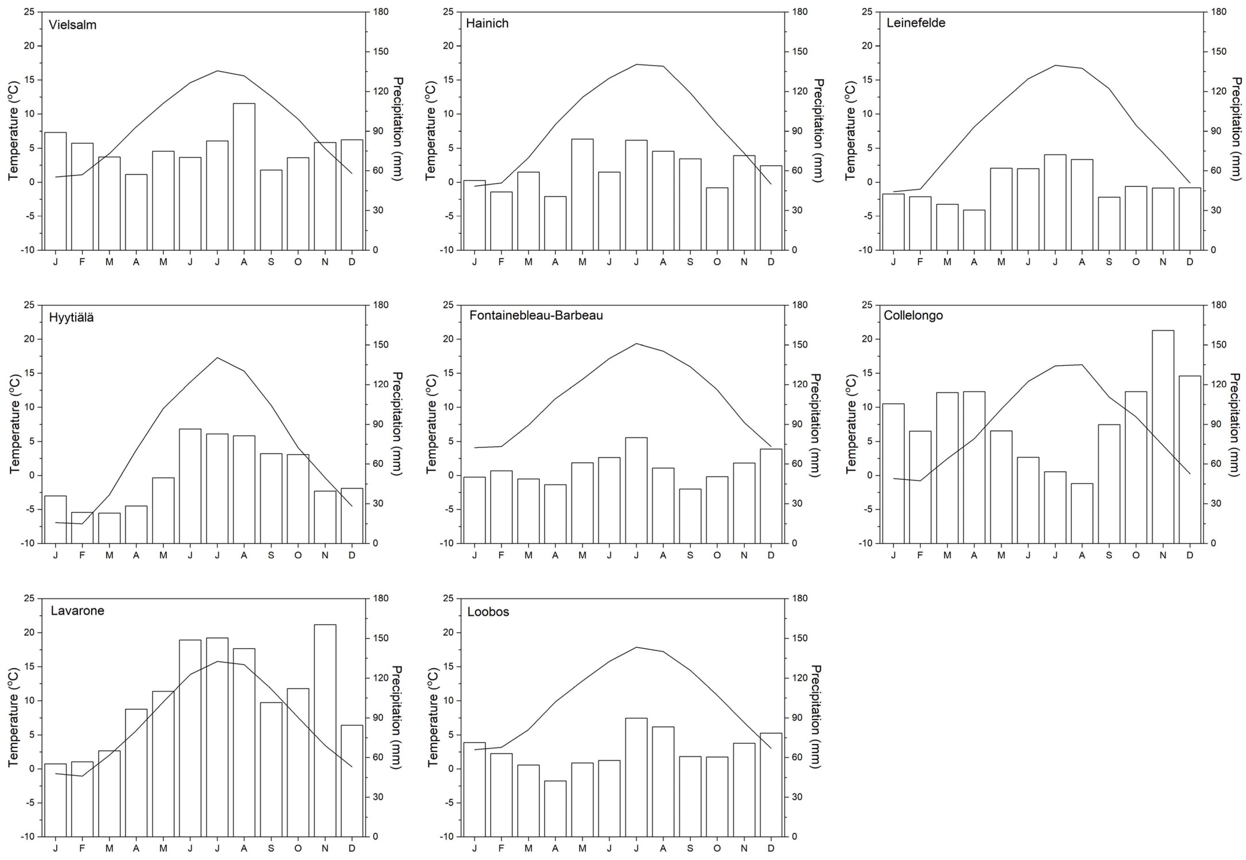
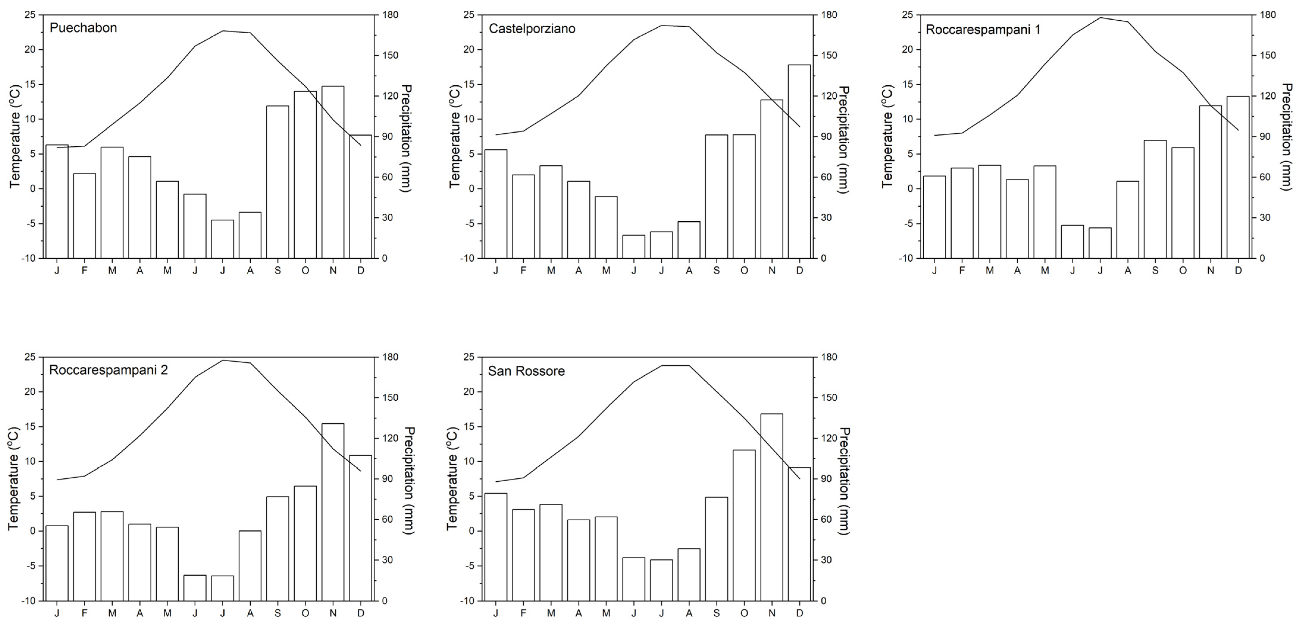
The evaluation of sCASE’s GPP estimates and the subsequent analyses were conducted across thirteen eddy covariance sites (Table 1). These sites differ markedly in their climatological characteristics, as reflected in their distribution across Europe (Figure 1) and in the average monthly temperature and precipitation patterns shown in Figure 2 and Figure 3. The sites can be grouped into two broad categories, those without summer water limitation and those that experience water limitation during summer. Eight sites fall into the first category, characterized by relatively low temperatures and evenly distributed precipitation throughout the year (Figure 2). In contrast, the remaining five sites experience summer water limitation due to the combined effects of high temperatures and low precipitation (Figure 3).

3.1. sCASE Evaluation

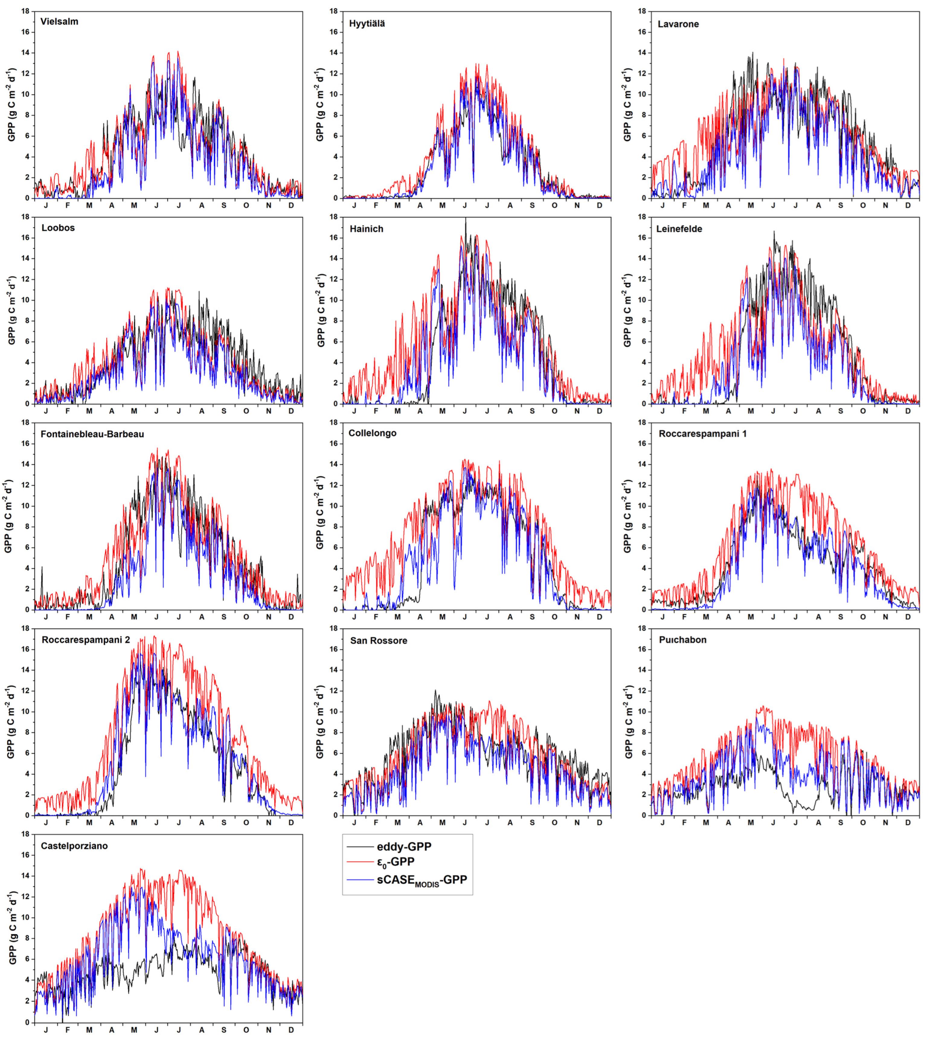
Using sCASE (Equation (2)), daily GPP values (g C m⁻² d⁻¹) were estimated for each study site (sCASE-GPP) and compared with the GPP measured by the eddy covariance towers (eddy-GPP). In addition, a simplified version of the LUE concept was applied to estimate GPP as the product of LUE_max and APAR (LUE_max-GPP), allowing an assessment of the influence of the three sCASE scalars. The seasonal dynamics of the three GPP estimates (eddy-GPP, sCASE-GPP, LUE_max-GPP) for an indicative year (2006) are shown in Figure 4. The time series clearly demonstrate that incorporating the three scalars substantially improves GPP estimation across all sites by reducing the pronounced overestimation produced by the LUE_max model (LUE_max-GPP). At most sites, sCASE slightly underestimates peak GPP values, whereas at the two evergreen broadleaf forest sites (Puéchabon and Castelporziano), it markedly overestimates GPP. For these two sites, sCASE does not adequately capture the magnitude or seasonal variability of GPP, particularly during spring and autumn, although it still performs better than the LUE_max-GPP approach.

The improved agreement of sCASE-GPP with the measured eddy-GPP, relative to the simple LUE_max-GPP approach, is also evident from the linear correlations between the modeled and observed GPP values. sCASE consistently exhibits higher R² and lower RMSE values than LUE_max-GPP (

Table 6. The coefficients of determination (R²) of the linear regressions and Root Mean Square Errors (RMSEs, g C m⁻² d⁻¹) between the two modeled GPPs (LUE_max-GPP and sCASE-GPP) and the measured eddy-GPP. All correlations are statistically significant (p-value < 0.001). Inside the parentheses, next to each site name, is the vegetation type according to IGBP (see Table 1).

	Study Site	LUEmax-GPP		sCASE-GPP
		R2	RMSE	R2	RMSE
Without Water Limitation	Vielsalm (MF)	0.776	1.960	0.787	2.380
	Hyytiälä (ENF)	0.838	1.391	0.875	1.391
	Lavarone (ENF)	0.641	2.510	0.692	2.940
	Loobos (ENF)	0.772	1.645	0.806	1.877
	Hainich (DBF)	0.764	2.495	0.855	2.291
	Leinefelde (DBF)	0.758	2.674	0.841	2.955
	Fontainebleau-Barbeau (DBF)	0.768	2.447	0.813	2.685
	Collelongo (DBF)	0.672	3.466	0.765	2.360
It is With Water Limitation	Roccarespampani 1 (DBF)	0.642	3.447	0.781	1.882
	Roccarespampani 2 (DBF)	0.656	4.127	0.767	2.264
	San Rossore (ENF)	0.600	2.162	0.669	2.202
	Puéchabon (EBF)	0.403	3.483	0.528	2.386
	Castelporziano (EBF)	0.483	3.858	0.564	2.507
	Average	0.675	2.746	0.750	2.317

), highlighting the substantial contribution of the three scalars. Across all sites, sCASE achieves higher R² values, yielding an average of 0.750 compared to 0.675 for LUE_max-GPP, and lower RMSE values for nearly all sites (average RMSE 2.317 g C m⁻² d⁻¹ versus 2.746 g C m⁻² d⁻¹). Overall, sCASE captures GPP variability reasonably well (Table 6), performing better at deciduous broadleaf and evergreen needleleaf forests (DBFs, ENFs) and less effectively at evergreen broadleaf forest (EBF) sites.

3.2. The Importance of Scalar Incorporation

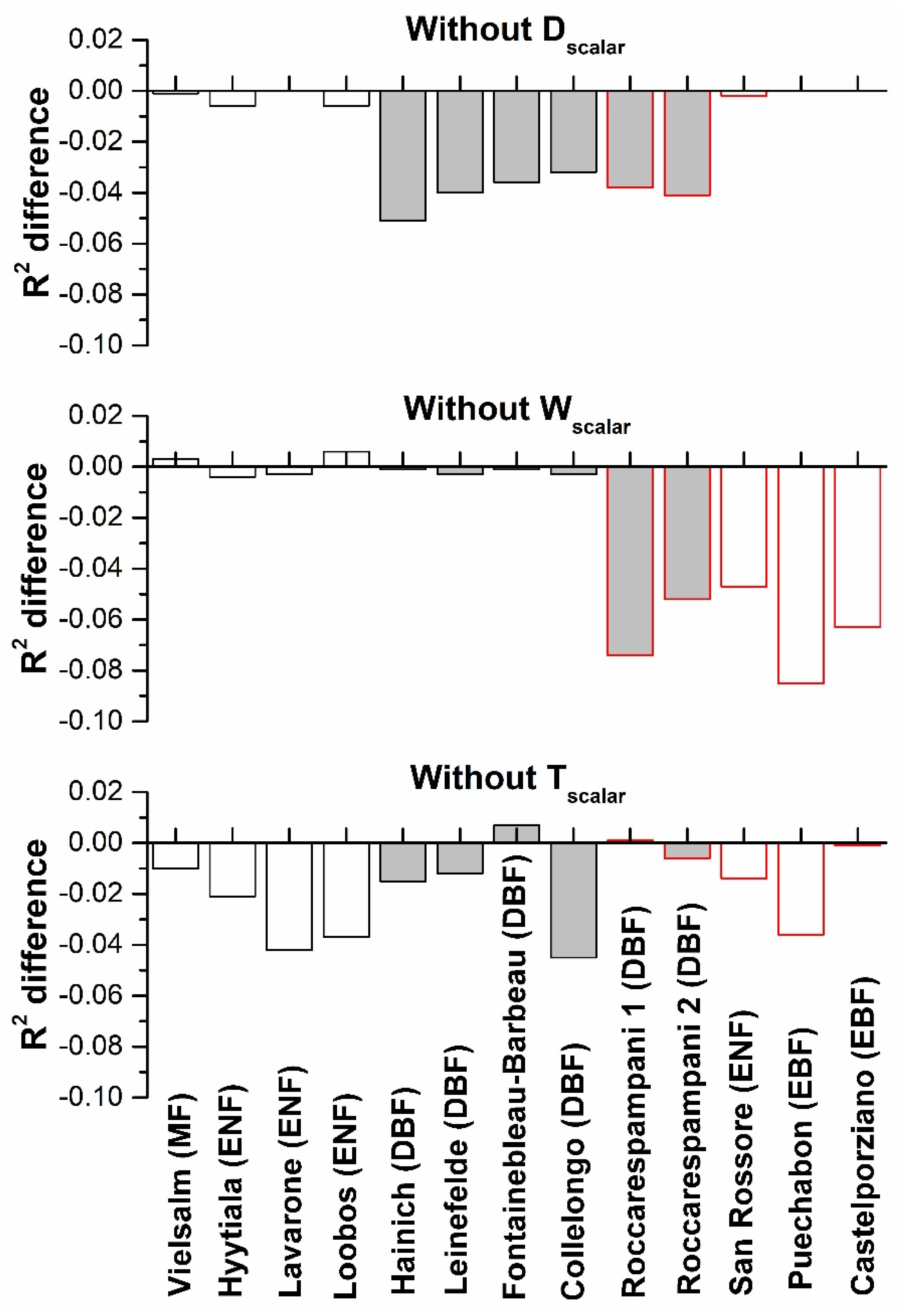
As shown above, the original sCASE algorithm improves GPP estimation by correcting the biases of the simple LUE_max-GPP approach through the downregulation of LUE by the three scalars (D_scalar, T_scalar and W_scalar). To further assess the contribution of each scalar, modified versions of the model were generated by removing one or more scalars from Equation (2).

Table 7. The coefficients of determination (R²) of the linear regressions between the variations of sCASE-GPP (scalar removal) and the measured eddy-GPP. All correlations are statistically significant (p-value < 0.001). Inside the parentheses, next to each site name, is the vegetation type according to IGBP. Sites with deciduous species (DBF) are highlighted with gray color.

	Study	Original	Without	Without	Without	Only	Only	Only
	Site	sCASE	Dscalar	Tscalar	Wscalar	Dscalar	Tscalar	Wscalar
Without Water Limitation	Vielsalm (MF)	0.787	0.786	0.777	0.790	0.783	0.789	0.769
	Hyytiälä (ENF)	0.875	0.868	0.854	0.870	0.852	0.865	0.839
	Lavarone (ENF)	0.692	0.692	0.651	0.690	0.648	0.690	0.644
	Loobos (ENF)	0.806	0.800	0.769	0.812	0.779	0.807	0.760
	Hainich (DBF)	0.855	0.804	0.840	0.855	0.841	0.808	0.758
	Leinefelde (DBF)	0.841	0.801	0.829	0.838	0.827	0.801	0.754
	Fontainebleau-Barbeau (DBF)	0.813	0.777	0.820	0.812	0.821	0.780	0.761
	Collelongo (DBF)	0.764	0.733	0.720	0.761	0.725	0.731	0.662
With Water Limitation	Roccarespampani 1 (DBF)	0.781	0.743	0.782	0.707	0.709	0.650	0.733
	Roccarespampani 2 (DBF)	0.767	0.726	0.761	0.715	0.707	0.676	0.704
	San Rossore (ENF)	0.669	0.667	0.655	0.622	0.602	0.621	0.653
	Puéchabon (EBF)	0.528	0.528	0.492	0.443	0.404	0.443	0.491
	Castelporziano (EBF)	0.564	0.564	0.563	0.501	0.483	0.500	0.562
	Average	0.750	0.730	0.732	0.724	0.706	0.705	0.699

presents the coefficient of determination (R²) between each GPP variant and the eddy-GPP. Using only a single scalar (any one of the three) substantially reduces model accuracy (average R² < 0.706 compared to 0.750 for the full model). Removing one scalar produces a smaller reduction in average accuracy, but the impact is pronounced at specific sites depending on their characteristics. In particular, removing the D_scalar reduces accuracy only at deciduous broadleaf forest (DBF) sites, while removing the W_scalar affects only the five sites that experience summer water limitation (Figure 5). The removal of the T_scalar primarily affects cold sites, especially those at high altitudes (Collelongo and Lavarone), but also influences two warm sites (Puéchabon and San Rossore). Overall, the full sCASE model provides the most robust performance, effectively integrating the diverse environmental controls on GPP.

3.3. Comparing the Different Water Scalars

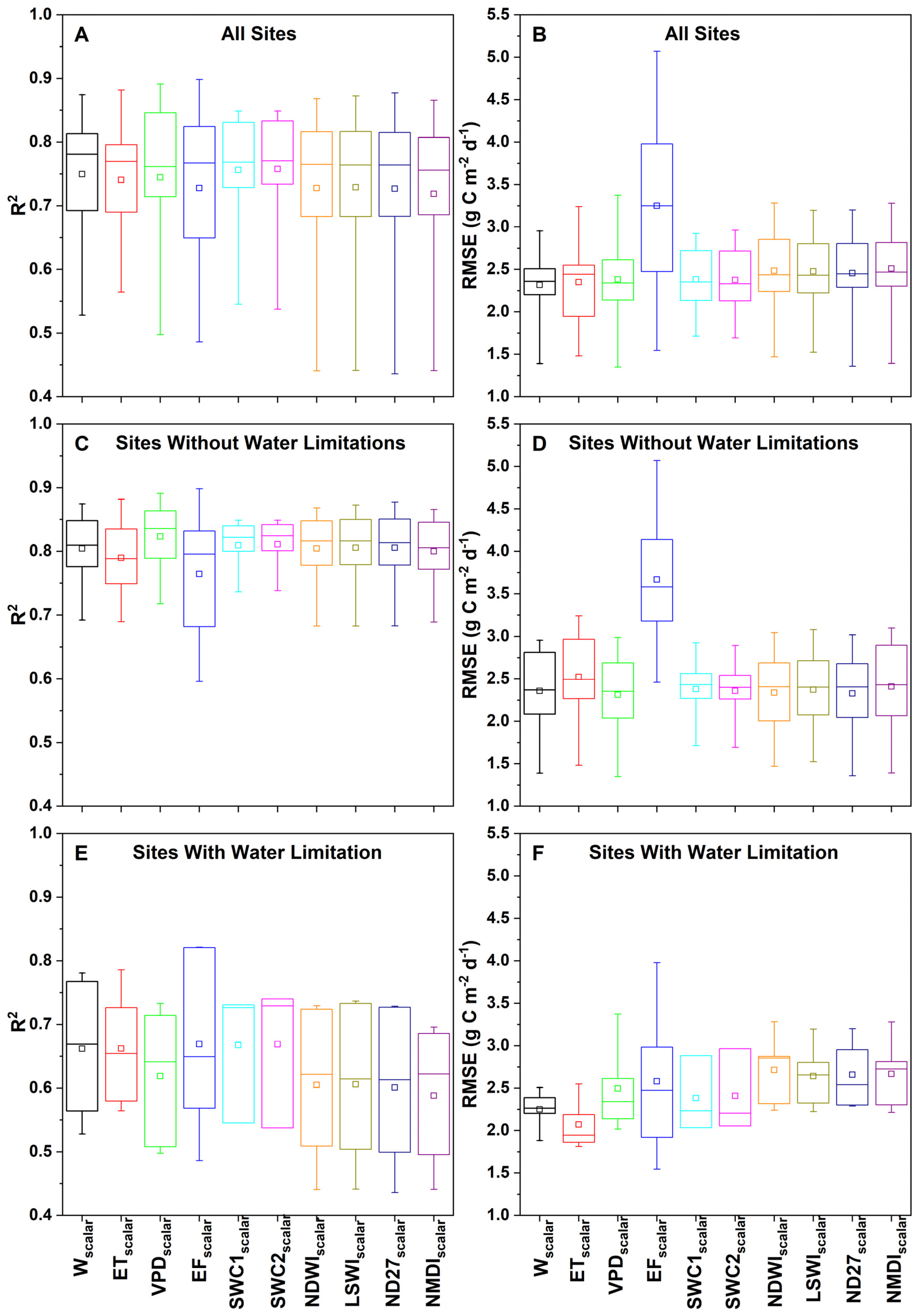
The final part of this study focuses on comparing a set of water scalars from the literature (Table 4), including the sCASE water scalar (W_scalar), to evaluate their ability to represent the effects of water status on photosynthesis and GPP. Variants of the sCASE model were generated by replacing W_scalar with each alternative water scalar while keeping the rest of the model structure (Equation (2)) unchanged. Daily GPP estimates from these model variants were then correlated with the eddy-GPP for each site. The resulting R² values are presented in

Table 8. The coefficients of determination (R²) of the linear regressions between the variations of sCASE (different water scalars) and the measured eddy-GPP. All correlations are statistically significant (p-value < 0.001). The intensity of the red color indicates the strength of the correlation, with the darker color corresponding to a higher R² value (for each row/site). Inside the parentheses, next to each site name, is the vegetation type according to IGBP (see Table 1).

	Study Site	W	ET	VPD	EF	SWC1	SWC2	NDWI	LSWI	ND27	NMDI
Without Water Limitation	Vielsalm (MF)	0.787	0.769	0.816	0.767	0.800	0.801	0.791	0.794	0.793	0.788
	Hyytiälä (ENF)	0.875	0.882	0.891	0.898	0.822	0.824	0.868	0.873	0.877	0.866
	Lavarone (ENF)	0.692	0.690	0.718	0.596			0.683	0.683	0.683	0.689
	Loobos (ENF)	0.806	0.781	0.826	0.826	0.737	0.738	0.816	0.816	0.812	0.804
	Hainich (DBF)	0.855	0.841	0.868	0.671	0.840	0.842	0.855	0.858	0.860	0.854
	Leinefelde (DBF)	0.841	0.829	0.859	0.838	0.849	0.849	0.841	0.842	0.842	0.837
	Fontainebleau-Barbeau (DBF)	0.813	0.796	0.846	0.824			0.816	0.817	0.815	0.807
	Collelongo (DBF)	0.764	0.729	0.762	0.693			0.765	0.764	0.764	0.756
With Water Limitation	Roccarespampani 1 (DBF)	0.781	0.786	0.733	0.821	0.731	0.729	0.724	0.733	0.727	0.686
	Roccarespampani 2 (DBF)	0.767	0.727	0.714	0.821	0.726	0.740	0.730	0.737	0.729	0.696
	San Rossore (ENF)	0.669	0.655	0.641	0.568			0.621	0.615	0.613	0.622
	Puéchabon (EBF)	0.528	0.580	0.498	0.649			0.441	0.441	0.436	0.441
	Castelporziano (EBF)	0.564	0.564	0.508	0.486	0.545	0.537	0.509	0.504	0.499	0.495
	Average	0.750	0.741	0.745	0.728	0.756	0.758	0.728	0.729	0.727	0.719

, and the corresponding RMSE values in

Table 9. The Root Mean Square Errors (RMSEs, g C m⁻² d⁻¹) between the GPP of the sCASE variations (different water scalars) and the measured eddy-GPP. The intensity of the red color indicates the magnitude of the RMSE, with the darker color corresponding to a lower RMSE (for each row/site). Inside the parentheses, next to each site name, is the vegetation type according to IGBP (see Table 1).

	Study Site	W	ET	VPD	EF	SWC1	SWC2	NDWI	LSWI	ND27	NMDI
Without Water Limitation	Vielsalm (MF)	2.380	2.495	2.311	3.879	2.270	2.263	2.378	2.374	2.364	2.399
	Hyytiälä (ENF)	1.391	1.481	1.350	2.462	1.714	1.692	1.471	1.522	1.360	1.391
	Lavarone (ENF)	2.940	2.925	2.846	5.070			3.044	3.080	3.018	2.976
	Loobos (ENF)	1.877	2.092	1.766	3.112	2.560	2.540	1.803	1.946	1.927	1.810
	Hainich (DBF)	2.291	2.488	2.331	4.224	2.433	2.401	2.205	2.205	2.160	2.466
	Leinefelde (DBF)	2.955	3.239	2.988	4.051	2.926	2.894	2.818	2.845	2.805	3.099
	Fontainebleau-Barbeau (DBF)	2.685	3.011	2.531	3.249			2.559	2.581	2.552	2.817
	Collelongo (DBF)	2.360	2.444	2.378	3.282			2.437	2.437	2.449	2.322
With Water Limitation	Roccarespampani 1 (DBF)	1.882	1.811	2.015	2.474	2.034	2.054	2.317	2.223	2.301	2.302
	Roccarespampani 2 (DBF)	2.264	2.187	2.341	1.920	2.233	2.204	2.873	2.803	2.294	2.725
	San Rossore (ENF)	2.202	2.550	2.139	3.980			2.240	2.323	2.289	2.214
	Puéchabon (EBF)	2.386	1.862	2.612	1.545			2.854	2.655	2.539	2.813
	Castelporziano (EBF)	2.507	1.947	3.374	2.983	2.882	2.964	3.281	3.195	3.200	3.280
	Average	2.317	2.349	2.383	3.248	2.381	2.377	2.483	2.476	2.455	2.509

. When examining model accuracy across all sites, differences in R² among the water scalar variants are relatively small, whereas RMSE varies more substantially (Figure 6A and Figure 6B, respectively). The average R² ranges from 0.719 (NMDI_scalar) to 0.758 (SWC2_scalar), while the average RMSE spans from 2.317 g C m⁻² d⁻¹ (W_scalar) up to 3.248 g C m⁻² d⁻¹ (EF_scalar).

Across the sites without summer water limitation, all water scalars perform similarly (Figure 6C,D), with the exception of EF_scalar, while the VPD_scalar shows a slightly higher average R² and a slightly lower RMSE. In contrast, at the five water-limited sites, W_scalar and ET_0scalar clearly outperform the other water scalars (Figure 6E,F). Between these two, ET_0scalar yields a lower average RMSE, whereas their R² values are nearly identical. The two scalars that incorporate the Soil Water Content (SWC1_scalar and SWC2_scalar) also show good overall performance, producing the highest average R² across all sites. However, this is partly due to the absence of SWC data at several sites with inherently low modeled/measured agreement (e.g., Puéchabon, San Rossore). Furthermore, the use of these two scalars results in higher RMSE values compared to the W_scalar (Table 9).

The four water scalars derived from MODIS indices perform unexpectedly well at the sites without summer water limitation, and their performance at the water-limited sites does not differ markedly from that of the other scalars (with the exception of W_scalar and ET_0scalar). Among the four, only NMDI_scalar shows slightly weaker performance. Finally, EF_scalar exhibits substantial variability across sites (Figure 6) and consistently produces high RMSE values, yielding by far the highest average RMSE (3.248 g C m⁻² d⁻¹). Although EF_scalar achieves very high R² values at some water-limited sites (Roccarespampani 1 and 2), it performs poorly at sites without water limitation (Lavarone and Hainich).

Overall, among the water scalars evaluated in this study, the sCASE W_scalar exhibited the best performance across all sites. At the water-limited sites, W_scalar and ET_0scalar performed markedly better than the other scalars, with ET_0scalar yielding the lowest average RMSE (for those sites). In contrast, at sites without water limitation, VPD_scalar proved to be the most suitable option.

4. Discussion

4.1. sCASE Evaluation

The GPP estimated by sCASE (sCASE-GPP) correlates well with the measured GPP (eddy-GPP) across the study sites (average R² = 0.750, average RMSE = 2.317 g C m⁻² d⁻¹), with the exception of the two evergreen broadleaf forest (EBF) sites (Puéchabon and Castelporziano). The moderate correlations observed at these sites are also evident (and even weaker) for the LUE_max-GPP (the product of LUE_max and APAR) estimates (Table 6). The GPP of Mediterranean EBF ecosystems is influenced by heat and water stress during summer but this does not seem to be the cause of the weak relationship of sCASE-GPP and eddy-GPP. On the contrary, sCASE drastically reduces GPP during summer at both sites, while the largest mismatch between modeled and measured GPPs appears during spring (Figure 4).

Similar patterns have been reported in numerous previous studies evaluating the performance of productivity models (not only LUE type) across different biomes [63,64,65]. For example, a comparison of four LUE models (EC-LUE, VPM, GLO-PEM and CASA) showed that all exhibited their lowest accuracy at EBF sites, based on both R² and RMSE metrics [66]. The difficulty in accurately modeling GPP in EBF ecosystems has been attributed to their weak or absent seasonal phenological signals, which are even less pronounced than in evergreen needleleaf species and complicate the representation of their functional dynamics [14,64,65,67]. Recent studies suggest that leaf age is a very important factor for EBF productivity and should be accounted for [68,69]. For improving EBF productivity modeling, future research is needed to understand their specific attributes.

Across all sites, incorporating the three scalars into the GPP estimation algorithm (the original sCASE formulation) resulted in stronger correlations (higher R²) with eddy-GPP than the simple LUE_max-GPP approach, although in a few cases, this came with slightly higher RMSE values (Table 6). Overall, the scalars clearly improve GPP estimation, yielding a higher average R² (0.750 for sCASE compared to 0.675 for LUE_max-GPP) and a lower average RMSE (2.317 g C m⁻² d⁻¹ vs. 2.746 of LUE_max-GPP). Nevertheless, the relationship between LUE_max-GPP and eddy-GPP remains relatively strong at most sites, supporting the fundamental principles of the light use efficiency framework [1,2].

Overall, sCASE demonstrated very good accuracy across the thirteen study sites, with R² values ranging from 0.528 to 0.875 and RMSE values from 1.391 to 2.955 g C m⁻² d⁻¹. Its performance was consistently superior to that of the MODIS LUE model (MOD17A2 product) at all sites (Appendix B), and comparable to the accuracy of widely used LUE models reported in the literature. For example, in an analysis comparing seven LUE models, Yuan et al. [65] found that the best-performing model (CFlux) produced R² values ranging from 0.000 (at an evergreen broadleaf forest) to 0.900 (at a deciduous broadleaf forest), with RMSE values between 0.525 g C m⁻² d⁻¹ (EBF) and 6.560 g C m⁻² d⁻¹ (DBF). Similarly, Zhang et al. [66] reported an average R² of 0.720 for the two best-performing models (VPM and GLO-PEM) across 31 forest sites. Although cross-study comparisons must be interpreted cautiously, these findings indicate that sCASE performs at a level comparable to the strongest LUE models evaluated in previous works.

The better performance of sCASE compared to the MODIS LUE model should be dealt with caution as MODIS GPP is known to have a moderate relationship with eddy-GPP [59,70,71,72]. The reasons for this are well documented, with the main factors being the species-specific parameters used, especially LUE_max [73,74], the meteorological input dataset [59,75], and fAPAR calculation [71,76].

Differences between LUE models arise primarily from their structural design (algorithm), while caution should be given to the parameters and input data used when different studies or GPP products (like the MOD17A2) are compared. Within the model structure, both the estimation of fAPAR and the regulation of LUE through scalars are critical determinants of accuracy [6,65,77], although the relative importance of each component varies by site characteristics [6]. While the method used to derive fAPAR from remote sensing data can influence GPP estimates [13,78,79], the LUE regulation component has received greater attention due to the wide diversity of indicators, equations, and number of limiting factors used in the literature [15,19]. Many LUE models employ only two scalars, typically for temperature and water availability, but previous studies have shown that incorporating additional limiting factors can improve model performance [19,65]. At the same time, the specific formulation and indicator used for each scalar can substantially affect model performance [15,66].

The number of scalars included in a LUE model should balance between under-representing key limiting processes when too few scalars are used, and introducing unnecessary complexity and parameterization requirements when too many are included [15]. Excessive scalar complexity can increase model uncertainty [80,81], and interactions among scalars may further amplify these uncertainties [15].

sCASE incorporates three scalars to downregulate LUE_max, and all three were found to enhance the overall accuracy of the model, with their relative importance determined by site-specific characteristics (Figure 5), consistent with findings from the forests of North Pindus [41]. Using only one of the three scalars substantially reduces model performance (Figure 5), underscoring the complex dependance of photosynthesis and productivity on multiple environmental factors. Each scalar is essential for certain sites, making their combined use necessary when applying a single algorithm across diverse ecosystems. Furthermore, even at sites where a given scalar is not strictly required, e.g., the W_scalar at water-abundant sites, its inclusion does not negatively affect the model performance.

The developmental scalar (D_scalar) was found to be essential for sites dominated by deciduous species, whereas it had no measurable effect on model accuracy at evergreen sites (Figure 5). As shown in Figure 4, LUE_max-GPP substantially overestimates productivity at deciduous sites during spring and winter, a bias that is considerably reduced in sCASE-GPP. Accurate timing of the start and end of the growing season and accurate representation of the photosynthetic rate during these transitional periods have been identified as a major source of discrepancy among GPP estimates [82,83,84].

The temperature scalar (T_scalar) influences model performance at many sites, particularly those with evergreen species and deciduous broadleaf forests (DBFs) exposed to cold conditions (Figure 5). However, because T_scalar also affects the two evergreen broadleaf forest (EBF) sites that experience summer heat stress, the use of the bell-shaped temperature response curve appears appropriate for capturing the effects of high temperatures on productivity. Although some studies argue that high-temperature effects need not be explicitly represented in the temperature scalar, on the assumption that they are already accounted for by the water scalar due to the link between heat and water limitation [4,24], the results of this study contradict that assumption, consistent with recent findings [19,85].

Finally, omitting the W_scalar leads to a pronounced decline in model accuracy at the five water-limited Mediterranean forest sites (Figure 5), underscoring the central role of water status in regulating LUE [65,86] and the importance of accurately detecting water stress for reliable GPP modeling in Mediterranean ecosystems [87].

4.2. Water Scalars Comparison

Although the importance of water status for accurate GPP estimation is well established, most studies assess water scalars only indirectly by comparing models that differ in multiple structural components. Such comparisons make it difficult to isolate the specific contribution of the water scalar itself. In contrast, the present study directly evaluates different water scalars, keeping the rest of the sCASE algorithm unchanged. Across the thirteen sites, the performance of the ten resulting GPP variants does not differ substantially (Table 8 and Table 9), with average R² values ranging from 0.719 to 0.758 and average RMSE values from 2.317 to 2.509 g C m⁻² d⁻¹ (with the exception of EF_scalar, which shows a much higher average RMSE 3.248 g C m⁻² d⁻¹). Based on both R² and RMSE, five scalars (W_scalar. ET_0scalar, VPD_scalar, SWC1_scalar and SWC2_scalar) perform slightly better than the others. Differences among scalars are minimal at sites without water limitation, where the VPD-based scalars show a modest advantage, but become more pronounced at water-limited sites, where water balance-based scalars (W_scalar and ET_0scalar) clearly outperform the rest.

The results clearly show that soil-based water scalars derived from the water balance are the most suitable for sites experiencing summer water limitation, whereas VPD, an atmospheric indicator, performs better at sites with ample water availability (Figure 6). This pattern has been repeatedly reported in the literature [88,89,90], and it is widely recognized that the optimal water indicator depends strongly on site ecohydrological characteristics [91,92]. In ecosystems where shallow soil layers dry rapidly and rooting depth is limited, soil moisture becomes the dominant constraint on photosynthesis, making soil-based indicators more effective. Conversely, in sites with deeper soil water storage, higher water holding capacity, or vegetation with strong hydraulic buffering, atmospheric demand (VPD) becomes the primary driver of stomatal regulation [93]. Thus, depending on soil texture, topography, vegetation structure and hydraulic traits as well as subsurface water storage, the dominant water-limiting mechanism may shift between soil dryness and atmospheric evaporative demand [94], subsequently determining which indicator best represents plant water stress. These ecohydrological differences also have implications for large-scale or operational GPP modeling: while VPD-based scalars are more robust to spatial data limitations and therefore more suitable for global applications, water balance-based scalars may provide more realistic stress estimates in regions where soil moisture limitation is the primary control on productivity.

The complex movement of water through the soil/plant/atmosphere continuum, influenced by soil texture and species-specific hydraulic strategies, further limits the ability of any single indicator to fully represent the effects of water status on photosynthesis [93,95,96]. Although recent studies have suggested that combining atmospheric- and soil-based water scalars may help address these limitations [19,97,98], the findings of this study do not support that assumption. The two scalars that combine VPD and SWC (SWC1_scalar and SWC2_scalar) do not outperform the single-indicator scalars. Their relatively high average R² values are largely attributable to the absence of SWC data at five sites, several of which exhibit low sCASE accuracy (e.g., Puéchabon). In comparison, VPD_scalar performs better at all non-water-limited sites, while sCASE’s W_scalar at all water-limited sites.

It is also important to note that SWC is often considered an unsuitable proxy for water status in forest ecosystems [21], as trees can access deeper water reserves that are not captured by SWC measurements restricted to the upper soil layers [99]. In contrast, the indirect estimation of soil water availability through the water balance appears to provide a more representative indicator for forested environments.

Water indicators of the plant category have often been proposed as the most suitable for representing water stress effects in GPP models [15,66], as they integrate both water supply and atmospheric demand. From this category, the present study evaluated one scalar based on the evaporative fraction (EF) and four scalars derived from MODIS water indices. EF_scalar appears particularly promising, showing high accuracy at many sites (Table 8) regardless of water status, and achieving the highest R² among all scalars at three of the five water-limited sites. However, EF_scalar also exhibits the weakest performance at six sites, producing the lowest R² values, and consistently yields high RMSE values, even at sites where correlations are strong (Table 9), differing greatly from the other water scalars. One possible explanation for this large site-to-site variability is the variable quality of the heat fluxes measurements across eddy covariance sites, as uncertainties in these measurements remain substantial [100,101]. The high RMSE values may also indicate that EF is not being incorporated optimally into the model, given that EF values are used directly as the water scalar.

Finally, the four sCASE variants that incorporate water scalars derived from MODIS indices perform comparably to the other sCASE variants at sites without water limitation, but show reduced accuracy at the water-limited sites (Figure 6), indicating that they fail to adequately capture the effects of water stress. Although the relationship between these indices and plant water content has been repeatedly observed [102], their ability to represent water stress impacts on large-scale photosynthesis remains debated [103]. Among the four, the NMDI_scalar variant exhibits the weakest performance (based on both R² and RMSE), whereas the remaining three show similar R² values, with ND27_scalar yielding the lowest RMSE (Table 9).

4.3. Model Up-Scaling

Although MODIS-derived water scalars are not ideal for water-limited environments, their overall accuracy, ease of implementation, and reliance on globally available datasets make them valuable tools for large-scale GPP modeling [6,21]. A major limitation of these scalars is the temporal frequency of the satellite indices, which varies among sensors and is often insufficient, particularly under atmospheric conditions that reduce data availability [14,15,24]. Spatial resolution is another critical factor, as it constrains the ability of these indices to capture fine-scale variability in vegetation water status, especially in regions with complex topography.

However, this limitation is even more critical for water scalars that rely on meteorological data, as it greatly constrains their applicability in large-scale model implementation. At the global scale, such data are typically derived either from spatial interpolation of ground-based measurements or from global meteorological models, both of which introduce substantial uncertainties that can affect model performance. Spatial interpolation relies on complex modeling approaches that incorporate multiple factors (e.g., topography) and can result in low data accuracy [104,105]. On the other hand, global meteorological datasets are provided at coarse spatial resolutions (often several kilometers), which reduces their representativeness for heterogenous landscapes [106]. The quality of meteorological inputs is therefore crucial for the performance of the corresponding water scalars, as numerous studies have shown that differences in meteorological datasets alone can lead to large discrepancies in modeled GPP [6,75,107].

Among the water indicators examined in this study, global-scale VPD data have been shown to agree well with ground-based measurements [108,109], which can explain why VPD is widely used as the primary water stress indicator in large-scale GPP modeling. VPD is also easier to estimate globally than soil moisture or heat flux variables, both of which are strongly influenced by topography and vegetation characteristics [110,111]. Nevertheless, the quality of large-scale soil moisture and heat flux datasets has improved in recent years, with several new products showing high accuracy [110,112,113]. Water balance-based scalars also face substantial challenges in global applications, as the estimation of ET₀ at broad spatial scales remains subject to considerable uncertainties [114].

In addition to the quality and availability of data, the implementation of sCASE (and productivity models in general) at a global scale will benefit from extensive physiological studies of species with different functional traits to support more accurate parameterization [15,65]. Understanding how different species use water and respond to water scarcity is essential for accurately monitoring productivity. Furthermore, insights into how species’ behavior varies with site-specific characteristics, such as aridity, can be used for the refinement of water scalars or the application of ecosystem-specific scalars.

5. Conclusions

sCASE proved to be an accurate model for estimating the gross primary productivity (GPP) across forest ecosystems with diverse functional and climatic characteristics, exhibiting higher accuracy in deciduous broadleaf forests and lower accuracy in evergreen broadleaf forests. Its overall performance was comparable to that of the most widely used LUE models reported in the literature. The three scalars used by sCASE to downregulate LUE (developmental, temperature and water) enhanced model accuracy, with the water scalar (W_scalar) exerting the strongest influence on GPP estimates. Special attention should be given to the developmental scalar, as it is absent from most LUE models despite its clear contribution to improving GPP estimation.

Based on the comparison of the different water scalars in this study, VPD-based scalars appear more suitable for sites with ample water availability, whereas water balance-based scalars more effectively capture the impacts of water stress on GPP in water-limited ecosystems. However, combining VPD (an atmospheric indicator) with a soil indicator did not improve model performance, contrary to suggestions from previous studies. EF_scalar exhibited very high performance at several sites across both water status categories, but its usefulness appears constrained by data quality issues. For large-scale applications, water scalars derived from MODIS indices offer the advantage of global coverage, which may outweigh their somewhat lower accuracy relative to other scalars.

References

1. Monteith, J.L. Solar Radiation and Productivity in Tropical Ecosystems. J. Appl. Ecol. 1972, 9, 747–766. [Google Scholar] [CrossRef]
2. Monteith, J.L. Climate and the Efficiency of Crop Production in Britain. Philos. Trans. R. Soc. Lond. B Biol. Sci. 1977, 281, 277–294. [Google Scholar] [CrossRef]
3. Goetz, S.J.; Prince, S.D. Modelling Terrestrial Carbon Exchange and Storage: Evidence and Implications of Functional Convergence in Light-Use Efficiency. Adv. Ecol. Res. 1999, 28, 57–92. [Google Scholar] [CrossRef]
4. Potter, C.S.; Randerson, J.T.; Field, C.B.; Matson, P.A.; Vitousek, P.M.; Mooney, H.A.; Klooster, S.A. Terrestrial Ecosystem Production: A Process Model Based on Global Satellite and Surface Data. Glob. Biogeochem. Cycles 1993, 7, 811–841. [Google Scholar] [CrossRef]
5. Prince, S.D.; Goward, S.N. Global Primary Production: A Remote Sensing Approach. J. Biogeogr. 1995, 22, 815. [Google Scholar] [CrossRef]
6. Zheng, Y.; Zhang, L.; Xiao, J.; Yuan, W.; Yan, M.; Li, T.; Zhang, Z. Sources of Uncertainty in Gross Primary Productivity Simulated by Light Use Efficiency Models: Model Structure, Parameters, Input Data, and Spatial Resolution. Agric. For. Meteorol. 2018, 263, 242–257. [Google Scholar] [CrossRef]
7. Yuan, W.; Liu, S.; Dong, W.; Liang, S.; Zhao, S.; Chen, J.; Xu, W.; Li, X.; Barr, A.; Andrew Black, T.; et al. Differentiating Moss from Higher Plants Is Critical in Studying the Carbon Cycle of the Boreal Biome. Nat. Commun. 2014, 5, 4270. [Google Scholar] [CrossRef]
8. Field, C.B.; Gamon, J.A.; Peñuelas, J. Remote Sensing of Terrestrial Photosynthesis. In Ecophysiology of Photosynthesis; Springer: Berlin/Heidelberg, Germany, 1995; pp. 511–527. [Google Scholar]
9. Hilker, T.; Coops, N.C.; Wulder, M.A.; Black, T.A.; Guy, R.D. The Use of Remote Sensing in Light Use Efficiency Based Models of Gross Primary Production: A Review of Current Status and Future Requirements. Sci. Total Environ. 2008, 404, 411–423. [Google Scholar] [CrossRef]
10. Landsberg, J.J.; Waring, R.H. A Generalised Model of Forest Productivity Using Simplified Concepts of Radiation-Use Efficiency, Carbon Balance and Partitioning. For. Ecol. Manag. 1997, 95, 209–228. [Google Scholar] [CrossRef]
11. Turner, D.P.; Urbanski, S.; Bremer, D.; Wofsy, S.C.; Meyers, T.; Gower, S.T.; Gregory, M. A Cross-Biome Comparison of Daily Light Use Efficiency for Gross Primary Production. Glob. Change Biol. 2003, 9, 383–395. [Google Scholar] [CrossRef]
12. Running, S.W.; Baldocchi, D.D.; Turner, D.P.; Gower, S.T.; Bakwin, P.S.; Hibbard, K.A. A Global Terrestrial Monitoring Network Integrating Tower Fluxes, Flask Sampling, Ecosystem Modeling and EOS Satellite Data. Remote Sens. Environ. 1999, 70, 108–127. [Google Scholar] [CrossRef]
13. Ruimy, A.; Kergoat, L.; Bondeau, A. Comparing Global Models of Terrestrial Net Primary Productivity (NPP): Analysis of Differences in Light Absorption and Light-Use Efficiency. Glob. Change Biol. 1999, 5, 56–64. [Google Scholar] [CrossRef]
14. Xiao, X.; Hollinger, D.; Aber, J.; Goltz, M.; Davidson, E.A.; Zhang, Q.; Moore, B. Satellite-Based Modeling of Gross Primary Production in an Evergreen Needleleaf Forest. Remote Sens. Environ. 2004, 89, 519–534. [Google Scholar] [CrossRef]
15. Pei, Y.; Dong, J.; Zhang, Y.; Yuan, W.; Doughty, R.; Yang, J.; Zhou, D.; Zhang, L.; Xiao, X. Evolution of Light Use Efficiency Models: Improvement, Uncertainties, and Implications. Agric. For. Meteorol. 2022, 317, 108905. [Google Scholar] [CrossRef]
16. Mahadevan, P.; Wofsy, S.C.; Matross, D.M.; Xiao, X.; Dunn, A.L.; Lin, J.C.; Gerbig, C.; Munger, J.W.; Chow, V.Y.; Gottlieb, E.W. A Satellite-Based Biosphere Parameterization for Net Ecosystem CO2 Exchange: Vegetation Photosynthesis and Respiration Model (VPRM). Glob. Biogeochem. Cycles 2008, 22, GB2005. [Google Scholar] [CrossRef]
17. Veroustraete, F.; Sabbe, H.; Eerens, H. Estimation of Carbon Mass Fluxes over Europe Using the C-Fix Model and Euroflux Data. Remote Sens. Environ. 2002, 83, 376–399. [Google Scholar] [CrossRef]
18. Turner, D.P.; Ritts, W.D.; Styles, J.M.; Yang, Z.; Cohen, W.B.; Law, B.E.; Thornton, P.E. A Diagnostic Carbon Flux Model to Monitor the Effects of Disturbance and Interannual Variation in Climate on Regional NEP. Tellus B 2006, 58, 476–490. [Google Scholar] [CrossRef]
19. Bao, S.; Wutzler, T.; Koirala, S.; Cuntz, M.; Ibrom, A.; Besnard, S.; Walther, S.; Šigut, L.; Moreno, A.; Weber, U.; et al. Environment-Sensitivity Functions for Gross Primary Productivity in Light Use Efficiency Models. Agric. For. Meteorol. 2022, 312, 108708. [Google Scholar] [CrossRef]
20. Lv, Y.; Liu, J.; He, W.; Zhou, Y.; Tu Nguyen, N.; Bi, W.; Wei, X.; Chen, H. How Well Do Light-Use Efficiency Models Capture Large-Scale Drought Impacts on Vegetation Productivity Compared with Data-Driven Estimates? Ecol. Indic. 2023, 146, 109739. [Google Scholar] [CrossRef]
21. Zhang, Y.; Song, C.; Sun, G.; Band, L.E.; Noormets, A.; Zhang, Q. Understanding Moisture Stress on Light Use Efficiency across Terrestrial Ecosystems Based on Global Flux and Remote-Sensing Data. J. Geophys. Res. Biogeosci. 2015, 120, 2053–2066. [Google Scholar] [CrossRef]
22. Nobel, P.S. Plants and Fluxes. In Physicochemical and Environmental Plant Physiology; Nobel, P.S., Ed.; Academic Press: Cambridge, MA, USA, 2009; pp. 438–505. [Google Scholar]
23. Yuan, W.; Liu, S.; Zhou, G.; Zhou, G.; Tieszen, L.L.; Baldocchi, D.; Bernhofer, C.; Gholz, H.; Goldstein, A.H.; Goulden, M.L.; et al. Deriving a Light Use Efficiency Model from Eddy Covariance Flux Data for Predicting Daily Gross Primary Production across Biomes. Agric. For. Meteorol. 2007, 143, 189–207. [Google Scholar] [CrossRef]
24. Xiao, X.; Zhang, Q.; Braswell, B.; Urbanski, S.; Boles, S.; Wofsy, S.; Moore, B.; Ojima, D. Modeling Gross Primary Production of Temperate Deciduous Broadleaf Forest Using Satellite Images and Climate Data. Remote Sens. Environ. 2004, 91, 256–270. [Google Scholar] [CrossRef]
25. Harley, P.C.; Thomas, R.B.; Reynolds, J.F.; Strain, B.R. Modelling Photosynthesis of Cotton Grown in Elevated CO2. Plant Cell Environ. 1992, 15, 271–282. [Google Scholar] [CrossRef]
26. Hall, D.O.; Rao, K.K. (Eds.) Photosynthesis, 5th ed.; Cambridge University Press: Cambridge, UK, 1994; ISBN 0521436222. [Google Scholar]
27. Le Quéré, C.; Andrew, R.; Friedlingstein, P.; Sitch, S.; Hauck, J.; Pongratz, J.; Pickers, P.; Ivar Korsbakken, J.; Peters, G.; Canadell, J.; et al. Global Carbon Budget 2018. Earth Syst. Sci. Data 2018, 10, 2141–2194. [Google Scholar] [CrossRef]
28. Bruhwiler, L.; Michalak, A.M.; Birdsey, R.; Fisher, J.B.; Houghton, R.A.; Huntzinger, D.N.; Miller, J.B. Overview of the Global Carbon Cycle. In Second State of the Carbon Cycle Report (SOCCR2): A Sustained Assessment Report; Cavallaro, N., Shrestha, G., Birdsey, R., Mayes, M.A., Najjar, R.G., Reed, S.C., Romero-Lankao, P., Zhu, Z., Eds.; U.S. Global Change Research Programl: Washington, DC, USA, 2018; pp. 42–70. [Google Scholar]
29. Zeng, J.; Matsunaga, T.; Tan, Z.H.; Saigusa, N.; Shirai, T.; Tang, Y.; Peng, S.; Fukuda, Y. Global Terrestrial Carbon Fluxes of 1999–2019 Estimated by Upscaling Eddy Covariance Data with a Random Forest. Sci. Data 2020, 7, 313. [Google Scholar] [CrossRef]
30. Ciais, P.; Reichstein, M.; Viovy, N.; Granier, A.; Ogée, J.; Allard, V.; Aubinet, M.; Buchmann, N.; Bernhofer, C.; Carrara, A.; et al. Europe-Wide Reduction in Primary Productivity Caused by the Heat and Drought in 2003. Nature 2005, 437, 529–533. [Google Scholar] [CrossRef]
31. Yuan, W.; Cai, W.; Chen, Y.; Liu, S.; Dong, W.; Zhang, H.; Yu, G.; Chen, Z.; He, H.; Guo, W.; et al. Severe Summer Heatwave and Drought Strongly Reduced Carbon Uptake in Southern China. Sci. Rep. 2016, 6, 18813. [Google Scholar] [CrossRef]
32. Anav, A.; Friedlingstein, P.; Beer, C.; Ciais, P.; Harper, A.; Jones, C.; Murray-Tortarolo, G.; Papale, D.; Parazoo, N.C.; Peylin, P.; et al. Spatiotemporal Patterns of Terrestrial Gross Primary Production: A Review. Rev. Geophys. 2015, 53, 785–818. [Google Scholar] [CrossRef]
33. Piao, S.; Nan, H.; Huntingford, C.; Ciais, P.; Friedlingstein, P.; Sitch, S.; Peng, S.; Ahlström, A.; Canadell, J.G.; Cong, N.; et al. Evidence for a Weakening Relationship between Interannual Temperature Variability and Northern Vegetation Activity. Nat. Commun. 2014, 5, 5018. [Google Scholar] [CrossRef]
34. Von Buttlar, J.; Zscheischler, J.; Rammig, A.; Sippel, S.; Reichstein, M.; Knohl, A.; Jung, M.; Menzer, O.; Altaf Arain, M.; Buchmann, N.; et al. Impacts of Droughts and Extreme-Temperature Events on Gross Primary Production and Ecosystem Respiration: A Systematic Assessment across Ecosystems and Climate Zones. Biogeosciences 2018, 15, 1293–1318. [Google Scholar] [CrossRef]
35. Zhu, X.; Zhang, S.; Liu, T.; Liu, Y. Impacts of Heat and Drought on Gross Primary Productivity in China. Remote Sens. 2021, 13, 378. [Google Scholar] [CrossRef]
36. Williams, S.E.; Bolitho, E.E.; Fox, S. Climate Change in Australian Tropical Rainforests: An Impending Environmental Catastrophe. Proc. R. Soc. B Biol. Sci. 2003, 270, 1887–1892. [Google Scholar] [CrossRef] [PubMed]
37. Nath, D.; Nath, R.; Chen, W. Faster Dieback of Rainforests Altering Tropical Carbon Sinks under Climate Change. npj Clim. Atmos. Sci. 2024, 7, 235. [Google Scholar] [CrossRef]
38. Albrich, K.; Seidl, R.; Rammer, W.; Thom, D. From Sink to Source: Changing Climate and Disturbance Regimes Could Tip the 21st Century Carbon Balance of an Unmanaged Mountain Forest Landscape. For. Int. J. For. Res. 2023, 96, 399–409. [Google Scholar] [CrossRef]
39. Au, J.; Bloom, A.A.; Parazoo, N.C.; Deans, R.M.; Wong, C.Y.S.; Houlton, B.Z.; Magney, T.S. Forest Productivity Recovery or Collapse? Model-Data Integration Insights on Drought-Induced Tipping Points. Glob. Change Biol. 2023, 29, 5652–5665. [Google Scholar] [CrossRef]
40. Conradi, T.; Eggli, U.; Kreft, H.; Schweiger, A.H.; Weigelt, P.; Higgins, S.I. Reassessment of the Risks of Climate Change for Terrestrial Ecosystems. Nat. Ecol. Evol. 2024, 8, 888–900. [Google Scholar] [CrossRef]
41. Stagakis, S.; Markos, N.; Vanikiotis, T.; Tzotsos, A.; Sykioti, O.; Kyparissis, A. SCASE: A Primary Productivity Monitoring System for the Forests of North Pindus National Park (Epirus, Greece). Eur. J. Remote Sens. 2015, 48, 223–243. [Google Scholar] [CrossRef]
42. Running, S.W.; Nemani, R.R.; Heinsch, F.A.; Zhao, M.; Reeves, M.; Hashimoto, H. A Continuous Satellite-Derived Measure of Global Terrestrial Primary Production. Bioscience 2004, 54, 547–560. [Google Scholar] [CrossRef]
43. Huang, X.; Lin, S.; Li, X.; Ma, M.; Wu, C.; Yuan, W. How Well Can Matching High Spatial Resolution Landsat Data with Flux Tower Footprints Improve Estimates of Vegetation Gross Primary Production. Remote Sens. 2022, 14, 6062. [Google Scholar] [CrossRef]
44. Chu, H.; Luo, X.; Ouyang, Z.; Chan, W.S.; Dengel, S.; Biraud, S.C.; Torn, M.S.; Metzger, S.; Kumar, J.; Arain, M.A.; et al. Representativeness of Eddy-Covariance Flux Footprints for Areas Surrounding AmeriFlux Sites. Agric. For. Meteorol. 2021, 301–302, 108350. [Google Scholar] [CrossRef]
45. Viovy, N.; Arino, O.; Belward, A.S. The Best Index Slope Extraction (Bise): A Method for Reducing Noise in NDVI Time-Series. Int. J. Remote Sens. 1992, 13, 1585–1590. [Google Scholar] [CrossRef]
46. Pastorello, G.; Trotta, C.; Canfora, E.; Chu, H.; Christianson, D.; Cheah, Y.W.; Poindexter, C.; Chen, J.; Elbashandy, A.; Humphrey, M.; et al. The FLUXNET2015 Dataset and the ONEFlux Processing Pipeline for Eddy Covariance Data. Sci. Data 2020, 7, 225. [Google Scholar] [CrossRef] [PubMed]
47. Howell, T.A.; Meek, D.W.; Hatfield, J.L. Relationship of Photosynthetically Active Radiation to Shortwave Radiation in the San Joaquin Valley. Agric. Meteorol. 1983, 28, 157–175. [Google Scholar] [CrossRef]
48. Reichstein, M.; Falge, E.; Baldocchi, D.; Papale, D.; Aubinet, M.; Berbigier, P.; Bernhofer, C.; Buchmann, N.; Gilmanov, T.; Granier, A.; et al. On the Separation of Net Ecosystem Exchange into Assimilation and Ecosystem Respiration: Review and Improved Algorithm. Glob. Change Biol. 2005, 11, 1424–1439. [Google Scholar] [CrossRef]
49. Papale, D.; Reichstein, M.; Aubinet, M.; Canfora, E.; Bernhofer, C.; Kutsch, W.; Longdoz, B.; Rambal, S.; Valentini, R.; Vesala, T.; et al. Towards a Standardized Processing of Net Ecosystem Exchange Measured with Eddy Covariance Technique: Algorithms and Uncertainty Estimation. Biogeosciences 2006, 3, 571–583. [Google Scholar] [CrossRef]
50. Vanikiotis, T.; Stagakis, S.; Kyparissis, A. Effects of Satellite Spatial Resolution on Gross Primary Productivity Estimation through Light Use Efficiency Modeling. In Proceedings of the SPIE—The International Society for Optical Engineering, Paphos, Cyprus, 26–29 March 2018; Volume 10773. [Google Scholar]
51. Tucker, C.J. Red and Photographic Infrared Linear Combinations for Monitoring Vegetation. Remote Sens. Environ. 1979, 8, 127–150. [Google Scholar] [CrossRef]
52. Roujean, J.L.; Breon, F.M. Estimating PAR Absorbed by Vegetation from Bidirectional Reflectance Measurements. Remote Sens. Environ. 1995, 51, 375–384. [Google Scholar] [CrossRef]
53. Allen, R.G.; Pereira, L.S.; Raes, D.; Smith, M. Crop Evapotranspiration: Guidelines for Computing Crop Requirements. Irrigation and Drainage Paper No. 56; FAO: Rome, Italy, 1998. [Google Scholar]
54. Running, S.; Zhao, M. User ’s Guide Daily GPP and Annual NPP (MOD17A2H/A3H) and Year-End Gap Filled (MOD17A2HGF/A3HGF) Products NASA Earth Observing System MODIS Land Algorithm (for Collection 6); MODIS Land Team: Greenbelt, MD, USA, 2019. [Google Scholar]
55. San-Miguel-Ayanz, J.; de Rigo, D.; Caudullo, G.; Houston Durrant, T.; Mauri, A. (Eds.) European Atlas of Forest Tree Species; Publication Office of the European Union: Luxembourg, 2016; Volume 11, ISBN 978-92-79-36740-3. [Google Scholar]
56. Heinsch, F.A.; Reeves, M.; Votava, P.; Kang, S.; Milesi, C.; Zhao, M.; Glassy, J.M.; Jolly, W.M.; Loehman, R.; Bowker, C.F.; et al. User’s Guide. GPP and NPP (MOD17A2/A3) Products NASA MODIS Land Algorithm; MODIS Land Team: Greenbelt, MD, USA, 2003. [Google Scholar]
57. Running, S.W.; Thornton, P.E.; Nemani, R.; Glassy, J.M. Global Terrestrial Gross and Net Primary Productivity from the Earth Observing System. In Methods in Ecosystem Science; Springer: New York, NY, USA, 2000; pp. 44–57. [Google Scholar]
58. Maselli, F.; Papale, D.; Puletti, N.; Chirici, G.; Corona, P. Combining Remote Sensing and Ancillary Data to Monitor the Gross Productivity of Water-Limited Forest Ecosystems. Remote Sens. Environ. 2009, 113, 657–667. [Google Scholar] [CrossRef]
59. Heinsch, F.A.; Zhao, M.; Running, S.W.; Kimball, J.S.; Nemani, R.R.; Davis, K.J.; Bolstad, P.V.; Cook, B.D.; Desai, A.R.; Ricciuto, D.M.; et al. Evaluation of Remote Sensing Based Terrestrial Productivity from MODIS Using Regional Tower Eddy Flux Network Observations. IEEE Trans. Geosci. Remote Sens. 2006, 44, 1908–1923. [Google Scholar] [CrossRef]
60. King, D.A.; Turner, D.P.; Ritts, W.D. Parameterization of a Diagnostic Carbon Cycle Model for Continental Scale Application. Remote Sens. Environ. 2011, 115, 1653–1664. [Google Scholar] [CrossRef]
61. Gao, B.C. NDWI—A Normalized Difference Water Index for Remote Sensing of Vegetation Liquid Water from Space. Remote Sens. Environ. 1996, 58, 257–266. [Google Scholar] [CrossRef]
62. Wang, L.; Qu, J.J. NMDI: A Normalized Multi-Band Drought Index for Monitoring Soil and Vegetation Moisture with Satellite Remote Sensing. Geophys. Res. Lett. 2007, 34, L20405. [Google Scholar] [CrossRef]
63. Raczka, B.; Davis, K.; Huntzinger, D.; Neilson, R.; Poulter, B.; Richardson, A.; Xiao, J.; Baker, I.; Ciais, P.; Keenan, T.; et al. Evaluation of Continental Carbon Cycle Simulations with North American Flux Tower Observations. Ecol. Monogr. 2013, 83, 531–556. [Google Scholar] [CrossRef]
64. Xie, X.; Li, A.; Tan, J.; Jin, H.; Nan, X.; Zhang, Z.; Bian, J.; Lei, G. Assessments of Gross Primary Productivity Estimations with Satellite Data-Driven Models Using Eddy Covariance Observation Sites over the Northern Hemisphere. Agric. For. Meteorol. 2020, 280, 107771. [Google Scholar] [CrossRef]
65. Yuan, W.; Cai, W.; Xia, J.; Chen, J.; Liu, S.; Dong, W.; Merbold, L.; Law, B.; Arain, A.; Beringer, J.; et al. Global Comparison of Light Use Efficiency Models for Simulating Terrestrial Vegetation Gross Primary Production Based on the LaThuile Database. Agric. For. Meteorol. 2014, 192–193, 108–120. [Google Scholar] [CrossRef]
66. Zhang, L.X.; Zhou, D.C.; Fan, J.W.; Hu, Z.M. Comparison of Four Light Use Efficiency Models for Estimating Terrestrial Gross Primary Production. Ecol. Model. 2015, 300, 30–39. [Google Scholar] [CrossRef]
67. Chang, X.; Xing, Y.; Gong, W.; Yang, C.; Guo, Z.; Wang, D.; Wang, J.; Yang, H.; Xue, G.; Yang, S. Evaluating Gross Primary Productivity over 9 ChinaFlux Sites Based on Random Forest Regression Models, Remote Sensing, and Eddy Covariance Data. Sci. Total Environ. 2023, 875, 162601. [Google Scholar] [CrossRef] [PubMed]
68. Yang, X.; Wu, J.; Chen, X.; Ciais, P.; Maignan, F.; Yuan, W.; Piao, S.; Yang, S.; Gong, F.; Su, Y.; et al. A Comprehensive Framework for Seasonal Controls of Leaf Abscission and Productivity in Evergreen Broadleaved Tropical and Subtropical Forests. Innovation 2021, 2, 100154. [Google Scholar] [CrossRef]
69. Tian, J.; Yang, X.; Yuan, W.; Lin, S.; Han, L.; Zheng, Y.; Xia, X.; Liu, L.; Wang, M.; Zheng, W.; et al. A Leaf Age-Dependent Light Use Efficiency Model for Remote Sensing the Gross Primary Productivity Seasonality over Pantropical Evergreen Broadleaved Forests. Glob. Change Biol. 2024, 30, e17454. [Google Scholar] [CrossRef] [PubMed]
70. de Almeida, C.T.; Delgado, R.C.; Galvão, L.S.; de Oliveira Cruz e Aragão, L.E.; Ramos, M.C. Improvements of the MODIS Gross Primary Productivity Model Based on a Comprehensive Uncertainty Assessment over the Brazilian Amazonia. ISPRS J. Photogramm. Remote Sens. 2018, 145, 268–283. [Google Scholar] [CrossRef]
71. Zhu, H.; Lin, A.; Wang, L.; Xia, Y.; Zou, L. Evaluation of MODIS Gross Primary Production across Multiple Biomes in China Using Eddy Covariance Flux Data. Remote Sens. 2016, 8, 395. [Google Scholar] [CrossRef]
72. Wang, L.; Zhu, H.; Lin, A.; Zou, L.; Qin, W.; Du, Q. Evaluation of the Latest MODIS GPP Products across Multiple Biomes Using Global Eddy Covariance Flux Data. Remote Sens. 2017, 9, 418. [Google Scholar] [CrossRef]
73. Martel, M.C.; Margolis, H.A.; Coursolle, C.; Bigras, F.J.; Heinsch, F.A.; Running, S.W. Decreasing Photosynthesis at Different Spatial Scales during the Late Growing Season on a Boreal Cutover. Tree Physiol. 2005, 25, 689–699. [Google Scholar] [CrossRef]
74. Wang, X.; Ma, M.; Li, X.; Song, Y.; Tan, J.; Huang, G.; Zhang, Z.; Zhao, T.; Feng, J.; Ma, Z.; et al. Validation of MODIS-GPP Product at 10 Flux Sites in Northern China. Int. J. Remote Sens. 2013, 34, 587–599. [Google Scholar] [CrossRef]
75. Zhao, M.; Running, S.W.; Nemani, R.R. Sensitivity of Moderate Resolution Imaging Spectroradiometer (MODIS) Terrestrial Primary Production to the Accuracy of Meteorological Reanalyses. J. Geophys. Res. 2006, 111, G01002. [Google Scholar] [CrossRef]
76. Zhao, M.; Heinsch, F.A.; Nemani, R.R.; Running, S.W. Improvements of the MODIS Terrestrial Gross and Net Primary Production Global Data Set. Remote Sens. Environ. 2005, 95, 164–176. [Google Scholar] [CrossRef]
77. Xiao, J.; Davis, K.J.; Urban, N.M.; Keller, K. Uncertainty in Model Parameters and Regional Carbon Fluxes: A Model-Data Fusion Approach. Agric. For. Meteorol. 2014, 189–190, 175–186. [Google Scholar] [CrossRef]
78. Cheng, Y.B.; Zhang, Q.; Lyapustin, A.I.; Wang, Y.; Middleton, E.M. Impacts of Light Use Efficiency and FPAR Parameterization on Gross Primary Production Modeling. Agric. For. Meteorol. 2014, 189–190, 187–197. [Google Scholar] [CrossRef]
79. Zhang, Y.; Hu, Z.; Wang, J.; Gao, X.; Yang, C.; Yang, F.; Wu, G. Temporal Upscaling of MODIS Instantaneous FAPAR Improves Forest Gross Primary Productivity (GPP) Simulation. Int. J. Appl. Earth Obs. Geoinf. 2023, 121, 103360. [Google Scholar] [CrossRef]
80. Medlyn, B.E.; Robinson, A.P.; Clement, R.; McMurtrie, R.E. On the Validation of Models of Forest CO2 Exchange Using Eddy Covariance Data: Some Perils and Pitfalls. Tree Physiol. 2005, 25, 839–857. [Google Scholar] [CrossRef] [PubMed]
81. Prentice, I.C.; Liang, X.; Medlyn, B.E.; Wang, Y.P. Reliable, Robust and Realistic: The Three R’s of next-Generation Land Surface Modelling. Atmos. Chem. Phys. Discuss. 2014, 14, 24811–24861. [Google Scholar] [CrossRef]
82. Falge, E.; Baldocchi, D.; Tenhunen, J.; Aubinet, M.; Bakwin, P.; Berbigier, P.; Bernhofer, C.; Burba, G.; Clement, R.; Davis, K.J.; et al. Seasonality of Ecosystem Respiration and Gross Primary Production as Derived from FLUXNET Measurements. Agric. For. Meteorol. 2002, 113, 53–74. [Google Scholar] [CrossRef]
83. Richardson, A.D.; Black, T.A.; Ciais, P.; Delbart, N.; Friedl, M.A.; Gobron, N.; Hollinger, D.Y.; Kutsch, W.L.; Longdoz, B.; Luyssaert, S.; et al. Influence of Spring and Autumn Phenological Transitions on Forest Ecosystem Productivity. Philos. Trans. R. Soc. B Biol. Sci. 2010, 365, 3227–3246. [Google Scholar] [CrossRef]
84. Richardson, A.D.; Anderson, R.S.; Arain, M.A.; Barr, A.G.; Bohrer, G.; Chen, G.; Chen, J.M.; Ciais, P.; Davis, K.J.; Desai, A.R.; et al. Terrestrial Biosphere Models Need Better Representation of Vegetation Phenology: Results from the North American Carbon Program Site Synthesis. Glob. Change Biol. 2012, 18, 566–584. [Google Scholar] [CrossRef]
85. Horn, J.E.; Schulz, K. Identification of a General Light Use Efficiency Model for Gross Primary Production. Biogeosciences 2011, 8, 999–1021. [Google Scholar] [CrossRef]
86. Tang, S.; Wang, X.; He, M.; Huang, L.; Zhang, Y.; Yang, H.; Piao, S. Global Patterns and Climate Controls of Terrestrial Ecosystem Light Use Efficiency. J. Geophys. Res. Biogeosci. 2020, 125, e2020JG005908. [Google Scholar] [CrossRef]
87. Moreno, A.; Maselli, F.; Chiesi, M.; Genesio, L.; Vaccari, F.; Seufert, G.; Gilabert, M.A. Monitoring Water Stress in Mediterranean Semi-Natural Vegetationwith Satellite and Meteorological Data. Int. J. Appl. Earth Obs. Geoinf. 2014, 26, 246–255. [Google Scholar] [CrossRef]
88. Xu, S.; Gentine, P.; Li, L.; Wang, L.; Yu, Z.; Dong, N.; Ju, Q.; Zhang, Y. Response of Ecosystem Productivity to High Vapor Pressure Deficit and Low Soil Moisture: Lessons Learned From the Global Eddy-Covariance Observations. Earth’s Future 2023, 11, e2022EF003252. [Google Scholar] [CrossRef]
89. Liu, L.; Gudmundsson, L.; Hauser, M.; Qin, D.; Li, S.; Seneviratne, S.I. Soil Moisture Dominates Dryness Stress on Ecosystem Production Globally. Nat. Commun. 2020, 11, 4892. [Google Scholar] [CrossRef] [PubMed]
90. Sun, X.; Xiao, Y.; Wang, J.; Zhou, M.; Song, Z.; Ma, M.; Han, X. The Respective Effects of Vapor Pressure Deficit and Soil Moisture on Ecosystem Productivity in Southwest China. Remote Sens. 2024, 16, 1316. [Google Scholar] [CrossRef]
91. Lv, Y.; He, W.; Liu, J.; Chen, H. Integration of Soil Moisture Factor into Light-Use Efficiency Models Improves Modeling Impact of Water Stresses on Gross Primary Production. Forests 2025, 16, 297. [Google Scholar] [CrossRef]
92. Wang, T.; Zhang, J.; Li, Z.; Lin, K.; Zhou, W.; Wu, G.; Pan, M.; Chen, X. Roles of Soil and Atmospheric Dryness on Terrestrial Vegetation Productivity in China—Which Dominates at What Thresholds. Earth’s Future 2025, 13, e2024EF005469. [Google Scholar] [CrossRef]
93. Wankmüller, F.J.P.; Delval, L.; Lehmann, P.; Baur, M.J.; Cecere, A.; Wolf, S.; Or, D.; Javaux, M.; Carminati, A. Global Influence of Soil Texture on Ecosystem Water Limitation. Nature 2024, 635, 631–638. [Google Scholar] [CrossRef]
94. Berauer, B.J.; Steppuhn, A.; Schweiger, A.H. The Multidimensionality of Plant Drought Stress: The Relative Importance of Edaphic and Atmospheric Drought. Plant. Cell Environ. 2024, 47, 3528–3540. [Google Scholar] [CrossRef]
95. Roman, D.T.; Novick, K.A.; Brzostek, E.R.; Dragoni, D.; Rahman, F.; Phillips, R.P. The Role of Isohydric and Anisohydric Species in Determining Ecosystem-Scale Response to Severe Drought. Oecologia 2015, 179, 641–654. [Google Scholar] [CrossRef] [PubMed]
96. Wang, X.; Guo, Z.; Zhang, K.; Fu, Z.; Lee, C.K.F.; Yang, D.; Detto, M.; Zhang, Y.; Wu, J. Can Large-Scale Satellite Products Track the Effects of Atmospheric Dryness and Soil Water Deficit on Ecosystem Productivity Under Droughts? Geophys. Res. Lett. 2025, 52, e2024GL110785. [Google Scholar] [CrossRef]
97. Stocker, B.D.; Wang, H.; Smith, N.G.; Harrison, S.P.; Keenan, T.F.; Sandoval, D.; Davis, T.; Prentice, I.C. P-Model v1.0: An Optimality-Based Light Use Efficiency Model for Simulating Ecosystem Gross Primary Production. Geosci. Model Dev. 2020, 13, 1545–1581. [Google Scholar] [CrossRef]
98. Wang, S.; Ibrom, A.; Bauer-Gottwein, P.; Garcia, M. Incorporating Diffuse Radiation into a Light Use Efficiency and Evapotranspiration Model: An 11-Year Study in a High Latitude Deciduous Forest. Agric. For. Meteorol. 2018, 248, 479–493. [Google Scholar] [CrossRef]
99. Schenk, H.J.; Jackson, R.B. Rooting Depths, Lateral Root Spreads and Below-ground/Above-ground Allometries of Plants in Water-limited Ecosystems. J. Ecol. 2002, 90, 480–494. [Google Scholar] [CrossRef]
100. Mauder, M.; Foken, T.; Cuxart, J. Surface-Energy-Balance Closure over Land: A Review. Bound. Layer Meteorol. 2020, 177, 395–426. [Google Scholar] [CrossRef]
101. Billesbach, D.P.; Arkebauer, T.J.; Sullivan, R.C. Intercomparison of Sensible and Latent Heat Flux Measurements from Combined Eddy Covariance, Energy Balance, and Bowen Ratio Methods above a Grassland Prairie. Sci. Rep. 2024, 14, 21866. [Google Scholar] [CrossRef]
102. Le, T.S.; Harper, R.; Dell, B. Application of Remote Sensing in Detecting and Monitoring Water Stress in Forests. Remote Sens. 2023, 15, 3360. [Google Scholar] [CrossRef]
103. Xiao, J. Assessing Net Ecosystem Exchange of Carbon Dioxide Between the Terrestrial Biosphere and the Atmosphere Using Fluxnet Observations and Remote Sensing. In Biophysical Applications of Satellite Remote Sensing; Hanes, J., Ed.; Springer: Berlin/Heidelberg, Germany, 2014; pp. 149–169. [Google Scholar]
104. Li, J.; Heap, A.D. A Review of Comparative Studies of Spatial Interpolation Methods in Environmental Sciences: Performance and Impact Factors. Ecol. Inform. 2011, 6, 228–241. [Google Scholar] [CrossRef]
105. Li, J.; Heap, A.D. Spatial Interpolation Methods Applied in the Environmental Sciences: A Review. Environ. Model. Softw. 2014, 53, 173–189. [Google Scholar] [CrossRef]
106. Peng, X.; She, J.; Zhang, S.; Tan, J.; Li, Y. Evaluation of Multi-Reanalysis Solar Radiation Products Using Global Surface Observations. Atmosphere 2019, 10, 42. [Google Scholar] [CrossRef]
107. Jung, M.; Vetter, M.; Herold, M.; Churkina, G.; Reichstein, M.; Zaehle, S.; Ciais, P.; Viovy, N.; Bondeau, A.; Chen, Y.; et al. Uncertainties of Modeling Gross Primary Productivity over Europe: A Systematic Study on the Effects of Using Different Drivers and Terrestrial Biosphere Models. Glob. Biogeochem. Cycles 2007, 21, GB4021. [Google Scholar] [CrossRef]
108. Fang, Z.; Zhang, W.; Brandt, M.; Abdi, A.M.; Fensholt, R. Globally Increasing Atmospheric Aridity Over the 21st Century. Earth’s Future 2022, 10, e2022EF003019. [Google Scholar] [CrossRef]
109. Wang, M.; Hu, Z.; Liu, X.; Hou, W. Vapor Pressure Deficit (VPD) Downscaling Based on Multi-Source Remote Sensing, in-Situ Observation, and Machine Learning in China. J. Hydrol. Reg. Stud. 2025, 57, 102192. [Google Scholar] [CrossRef]
110. Lu, Y.; Steele-Dunne, S.C.; De Lannoy, G.J.M. Improving Soil Moisture and Surface Turbulent Heat Flux Estimates by Assimilation of SMAP Brightness Temperatures or Soil Moisture Retrievals and GOES Land Surface Temperature Retrievals. J. Hydrometeorol. 2020, 21, 183–203. [Google Scholar] [CrossRef]
111. He, J.; Li, Q.M.; Wang, W.C.; Xu, D.M.; Wan, Y.R. The Diurnal Variation Characteristics of Latent Heat Flux under Different Underlying Surfaces and Analysis of Its Drivers in The Middle Reaches of the Heihe River. Water 2022, 14, 3514. [Google Scholar] [CrossRef]
112. Liu, Y.; Zha, Y.; Ran, G.; Zhang, Y.; Shi, L. SMRFR: A Global Multilayer Soil Moisture Dataset Generated Using Random Forest from Multi-Source Data. Sci. Data 2025, 12, 1170. [Google Scholar] [CrossRef] [PubMed]
113. Ford, T.W.; Quiring, S.M. Comparison of Contemporary In Situ, Model, and Satellite Remote Sensing Soil Moisture With a Focus on Drought Monitoring. Water Resour. Res. 2019, 55, 1565–1582. [Google Scholar] [CrossRef]
114. Sun, S.; Xu, S.; Li, L.; Lin, Y.; Liu, H.; Maggioni, V.; Xu, Y.; Fu, C. Global Assessment of Terrestrial Precipitation and Evapotranspiration in CMIP6 Simulations Using Observation-Based Estimates. Front. Water 2025, 7, 1520258. [Google Scholar] [CrossRef]
Figure 1. The thirteen sites with eddy covariance towers. Background map Google Satellite (Imagery © 2024 TerraMetrics, Map Data © 2024).
Remotesensing 18 00548 g001
Figure 2. Average monthly temperature and precipitation of the eight study sites without water limitation.
Remotesensing 18 00548 g002
Figure 3. Average monthly temperature and precipitation of the five study sites with water limitation.
Remotesensing 18 00548 g003
Figure 4. Daily GPP values for the thirteen study sites as measured by the eddy covariance towers (eddy-GPP) and estimated by sCASE (sCASE-GPP) and the LUEmax model (LUEmax-GPP), for the year 2016.
Remotesensing 18 00548 g004
Figure 5. The difference between the R2 of the original sCASE and the three variations of the model that lack one of the scalars, for the thirteen sites. The sites with deciduous species (DBF) are highlighted with gray color and the sites with water limitation are highlighted with red outlines.
Remotesensing 18 00548 g005
Figure 6. Boxplots of the coefficients of determination (R2) of the linear regressions and Root Mean Square Errors (RMSEs, g C m−2 d−1) between the variations of sCASE (different water scalars) and the measured eddy-GPP. (A,B) concern all the sites, (C,D) the sites without water limitation and (E,F) the sites with water limitation.
Remotesensing 18 00548 g006