


Highlights
What are the main findings?
- Consistent DHIs–richness associations across two independent richness products: (i) SDM-based richness and (ii) IUCN range map richness. Across habitat guilds, RF achieved R2adj = 0.57–0.73 for SDM-based richness and R2adj = 0.68–0.71 for IUCN-based richness (p < 0.001).
- Random Forest consistently delivered the best predictive performance for both overall and guild-specific richness, improving R2adj by +1.8–7.1% vs. GAM (SDM; mean +4.6%) and +7.7–10.9% vs. GAM (IUCN; mean +8.9%) across guilds.
What are the implications of the main findings?
- This work suggests that satellite-derived DHIs provide a robust and scalable proxy for large-scale biodiversity monitoring.
- The results have important implications for conservation planning, highlighting the role of maintaining habitat productivity in supporting resident bird diversity under ongoing environmental change.
Abstract
Dynamic Habitat Indices (DHIs) are crucial for understanding species richness patterns and provide a powerful tool for large-scale biodiversity conservation research. DHIs summarize three key aspects of vegetation productivity: (a) cumulative annual productivity, (b) minimum productivity, and (c) intra-annual variability. While DHIs have demonstrated potential for predicting richness patterns globally and in tropical regions, their predictive ability across climate zones and using multiple sources of species richness data remains untested. We assess the feasibility of using DHIs to predict the richness of resident birds in China and explore approaches to improve model performance. We used (a) IUCN range maps of terrestrial resident birds in China, and (b) species distribution models (SDMs) to delineate bird richness patterns, classifying species into six habitat guilds: forest, shrubland, grassland, cropland, wetland, and all resident birds. We linked DHIs to richness in each guild and quantified their predictive power using three modeling approaches: linear (GLM) and non-linear models (GAM, Random Forest). We also recorded the relative importance of each DHI component in the models. Our results show that DHIs best predicted cropland bird richness (SDM-based richness, adjusted R2 = 0.73), while for IUCN-based guilds, adjusted R2 ranged from 0.68 to 0.71. The Random Forest model achieved the highest performance and interpretability. Among DHI components, cumulative DHI consistently played the most dominant role in predicting richness from both SDM and IUCN sources. DHIs effectively capture the link between energy availability and resident bird richness in China, demonstrating considerable potential for biodiversity assessment and conservation planning.
1. Introduction
Over the past century, rapid population growth and intensifying demands for economic development—together with land-use change and accelerating habitat degradation—have imposed severe pressures on habitats and species richness; consequently, global biodiversity has been declining at an alarming rate [1,2,3,4]. Understanding, and being able to predict species richness along natural environmental gradients is essential for characterizing and monitoring contemporary biodiversity patterns, detecting change and its potential drivers, forecasting future dynamics, and identifying appropriate conservation strategies [5,6,7]. At broad scales, biodiversity patterns are driven by three principal determinants [8]: climatic stability [9], productivity [10], and habitat structure [11]. The link between productivity and species diversity is one of macroecology’s long-standing foci. The classic species–energy hypothesis posits that higher primary productivity provides greater resource supply, enabling the coexistence of more populations and thereby increasing regional species diversity [12,13]. Support is strong for vascular plants at regional-to-continental extents, where energy/productivity explains broad spatial gradients in richness [14,15]. Across these broad extents, richness is jointly constrained by energy and water availability, with their relative contributions varying among regions and taxa [16,17,18]. Beyond terrestrial plants, parallel energy–diversity links have been documented in marine microbial systems, extending the generality of the pattern across realms [19]. This hypothesis has received extensive empirical support worldwide.
Satellite remote sensing provides long time series of spatial information on attributes closely linked to biodiversity—such as large-scale habitat structure, ecological processes and functions—and has become a key technology for biodiversity monitoring and assessment [20,21,22]. Although productivity-based proxies can be affected by saturation effects, biome-specific nonlinear relationships, and potential decoupling between productivity and biodiversity in human-modified landscapes, remote sensing remains an essential tool for large-scale biodiversity research. Methods for remote-sensing-based biodiversity monitoring are generally divided into direct and indirect approaches [23]: the former detects or observes species and communities with sensors, whereas the latter uses habitat productivity and other characteristics as proxies to evaluate biodiversity patterns. A series of vegetation parameters derived from satellite datasets can retrieve information on terrestrial productivity from outer space. For example, the Normalized Difference Vegetation Index (NDVI) and the Enhanced Vegetation Index (EVI), which quantify the contrast between red-band absorption and near-infrared reflectance, have been widely proved to be significantly correlated with species richness [24,25,26,27,28]. However, applying vegetation indices as proxies for productivity is often challenging when it comes to accurately capturing changes and differences in primary productivity [29,30].
Metrics such as Leaf Area Index (LAI) [31], the fraction of Absorbed Photosynthetically Active Radiation (fPAR) [32,33] and Gross Primary Productivity (GPP) [34,35,36,37,38] provide more direct observations of productivity patterns. Species richness mapping is crucial for understanding past and current community states and for anticipating potential shifts in distributions under future scenarios [39,40]. When combined with satellite remote sensing, such mapping enables better identification of key environmental variables, clarifies the determinants of biodiversity, and supports biodiversity conservation and policy-making [41,42,43,44].
We hypothesize that regions with higher productivity support greater species diversity; satellite-derived measures of vegetation productivity provide the means to test this relationship consistently across large spatial extents. The Dynamic Habitat Indices (DHIs) establish relationships between terrestrial primary productivity and species richness from a satellite remote sensing perspective, focusing on three dimensions: the Available Energy Hypothesis, the Environmental Stability Hypothesis, and the Environmental Stress Hypothesis. This framework is intended to explain the geographical patterns of species diversity. The productivity–diversity hypothesis posits that regions with higher productivity support greater biodiversity [45,46,47]. At least three conditions are required to support this expectation. (a) Higher energy input (either potential or chemical energy). This mechanism underpins the Available Energy Hypothesis, which posits that energy supply sets an upper bound on standing richness by increasing individual abundance, relaxing demographic stochasticity, and enlarging the viable niche space at broad spatial extents [48,49,50]. (b) Lower environmental seasonality. These processes are formalized in the Environmental Stability Hypothesis, which asserts that persistently low seasonality lengthens the effective windows for growth and reproduction and fosters niche partitioning and specialization, thereby elevating richness [48,49]. (c) Lower environmental stress. This logic is captured by the Environmental Stress Hypothesis: chronic or acute stress raises maintenance costs, narrows tolerable niche space, and elevates local extinction risk, whereas higher minimum energy mitigates these bottlenecks and supports greater richness [51]. Correspondingly, the three DHIs (a) Cumulative DHI; (b) Variation DHI; (c) Minimum DHI serve as remote-sensing-based proxies for large-scale assessments of available energy, environmental stability, and environmental stress, respectively [52].
The Dynamic Habitat Indices (DHIs) were first proposed in Australia [53] and have subsequently been applied in Canada [54,55,56], North America [57], and China [58]. At the global scale, the relationship between DHIs and species richness has been well established: DHIs can explain over 60% of the spatial variation in amphibian, birds, and mammal richness, demonstrating consistency across taxonomic groups [59,60]. They have also revealed differences in the sensitivity of richness patterns to the three DHI components-cumulative productivity (DHIcum), minimum productivity (DHImin), and seasonality (DHIvar) among different biogeographic regions [61]. At regional scales and across functional groups, studies in North America have shown that DHIs are strongly associated with avian species richness, with seasonal variation in satellite-derived vegetation greenness (e.g., NDVI, EVI, FVC) and spatial heterogeneity in greenness being key variables for explaining richness patterns. Combining topography and climate variables with DHIs significantly improves explanatory power for grassland and woodland breeding birds [62,63,64]. The incorporation of Land Surface Temperature (LST) index can further enhance model predictive capacity [65]. The reliance on specific DHI components varies by region and functional group: in Ontario, Canada, Minimum DHI is most critical for breeding birds, especially grassland species [52], while in tropical regions, Cumulative DHI makes the greatest contribution to resident bird richness in Thailand [66]. Joint modelling of DHIs with topographic and climatic variables generally yields complementary rather than redundant effects, as has been demonstrated for the Mongolian Plateau [67]. In China, the cross-taxon consistency of DHIs with species richness has also been confirmed, and significant associations have been found between DHIs and human activity [68]. Beyond avians, DHIs have also been shown to effectively characterize other taxa, such as: butterfly diversity in Canada is significantly positively correlated with both Cumulative and Minimum DHI [69], and successful predictions have been made for large mammals, including wild moose population in Northeast China and Russia [70,71,72].
In terms of remote-sensing hardware, the cross-sensor consistency of DHIs has been validated: results derived from different MODIS vegetation products are comparable, and with appropriate calibration, key features derived from different sensors (such as interannual stability) have been shown to exhibit high temporal consistency. This supports the application of multi-product DHI calculation to extend analyses over finer spatial scales and higher resolutions than possible for single MODIS products [60,73]. Moreover, constructing and comparing DHIs based on multi-source GPP data can help test their robustness and explanatory power [74]. At the spatial scale, multi-granularity image fusion has been shown to outperform single-resolution models in explaining and predicting avian species richness [75]. High-resolution image collections based on Landsat and Sentinel-2 also provide new opportunities for biodiversity monitoring with both fine granularity and long temporal coverage [76]. To date, however, there is still a lack of studies that systematically examine the relationship between DHIs and species richness using multi-source richness data across large-scale regions with complex biodiversity gradients, in order to fully assess the potential of DHIs for biodiversity monitoring.
However, differences in construction assumptions and spatial grain across richness products can introduce systematic biases when modelling and predicting with remote-sensing proxies. Species distribution model (SDM)-based richness and IUCN range-map richness reflect fundamentally different assumptions about how the environment shapes species distributions. SDM-based richness is derived by stacking environment-driven models for individual species onto a common grid [77,78], making it particularly responsive to local variation in energy and seasonality, as captured by DHIs. Nevertheless, SDM richness simulated from occurrence records may be subject to sampling bias, as records can be more concentrated in areas with higher accessibility rather than where species actually occur, which may affect the selection of background points/pseudo-absences [79] and model fitting. In contrast, IUCN range map is obtained by overlaying expert-drawn range polygons that are typically coarser in resolution, may encompass areas not actually occupied by the species, and are less sensitive to fine-scale environmental heterogeneity; because range maps are intended to depict the maximum geographic distribution [80], stacking multiple species’ range maps may overestimate richness in some areas. These biases can affect the interpretability of the model.
Despite the exciting progress made in applying Dynamic Habitat Indices to global biodiversity research, several limitations remain. First, the application and validation of DHIs at the national scale, particularly across regions with broad biodiversity gradients, have remained relatively limited. Second, in settings spanning multiple climate zones, previous studies have rarely examined within a unified framework how species richness derived from species distribution models (SDMs) and IUCN range maps differ in their responses to productivity-based indicators. Third, the contributions of the three DHI components to biodiversity patterns require further scrutiny. Finally, systematic comparisons across modelling frameworks have remained insufficient, especially regarding model selection and the interpretability of predictors.
Our objective is to assess the feasibility of using satellite-derived Dynamic Habitat Indices (DHIs) to evaluate terrestrial resident bird richness across China, to investigate differences and effectiveness among various sources of richness data, and to identify the optimal model for linking DHIs with resident bird richness. Specifically, we aim to:
- (a)
- validate the relationships between different sources of DHIs and terrestrial resident bird richness;
- (b)
- compare two types of richness products—modelled richness based on species distribution models (SDMs) and richness estimated from IUCN range maps—in terms of their correlation with and explanatory power for DHIs (indicators of the reliability of DHIs as proxies for bird richness);
- (c)
- evaluate the performance of various modelling approaches in establishing the relationship between DHIs and richness (and different guilds), and to identify an appropriate modelling framework, assess the relative importance of DHI components in prediction (to identify where DHIs may be more or less reliable proxies for richness).
2. Materials and Methods
2.1. Overview of the Study Area
China is located in East Asia and covers a total land area of approximately 9.6 million km2. The country exhibits a stepped topography, sloping from the highlands in the west to the lowlands in the east, with striking elevation differences (ranging from −154 m to 8848.86 m). The landscape encompasses a complex array of plains, plateaus, mountains, hills, and both large and small basins. Precipitation and temperature exhibit pronounced spatial gradients across China. Annual precipitation spans 100–2000 mm. The seasonal mean temperature varies between −2.8–22.3 °C, and the growing-season accumulated temperature is 2000–7000 °C·d. The combination of this varied topography and broad latitudinal span together encompasses climatic zones from cold-temperate to tropical, thereby shaping pronounced spatial heterogeneity in ecosystems.
As one of the world’s most biodiverse countries, China is home to over 130,000 species, including more than 2700 terrestrial vertebrates and a large number of endemic species [81], accounting for more than one-eighth of global totals. For birds, more than 1500 species have been recorded in China, with over 70 species endemic to the country [82]. Although habitat loss caused by intensified human activities over the past half-century has threatened to 10.6% of bird species [83], the situation has significantly improved as a result of the development of a comprehensive protected area network and the robust implementation of national ecological conservation policies [84].
2.2. Dynamic Habitat Indices, DHIs
To capture intra-annual variation in habitat productivity, this study constructed 1-km Dynamic Habitat Indices (DHIs) for China using Google Earth Engine (https://code.earthengine.google.com, 8 January 2024), based on MODIS vegetation production datasets (NDVI/EVI: MOD13Q1; FPAR/LAI: MCD15A3H) and GPP (PML_V2_v0.1.8). Time series imagery from 2012 to 2023 for China was used to generate monthly composite images on a per-pixel basis using median compositing. Three DHI components were then calculated: Cumulative DHI (DHIcum), Variation DHI (DHIvar), and Minimum DHI (DHImin). The Dynamic Habitat Indices reflect three dimensions of intra-annual habitat productivity, representing the levels of available energy, environmental stability, and environmental stress, respectively (Figure 1).
Figure 1.
Spatial distribution patterns of Dynamic Habitat Indices (DHIs) across China based on 2020 GPP data: (a) color composite of the three DHI components; (b) Cumulative DHI; (c) Variation DHI; (d) Minimum DHI.
To eliminate interference from non-productive (e.g., water, snow, ice, desert) pixels, we utilized water body boundaries [85] provided by the National Cryosphere Desert Data Center (http://www.ncdc.ac.cn, 10 February 2024) in combination with the no-data ranges of DHIvar and other imagery to generate a mask. This mask was applied to all DHIs datasets.
2.3. Bird Distribution Data
Migratory and resident birds exhibit structural differences in how they respond to climate and vegetation. Compared with migratory and breeding species that undertake cross-border movements, resident birds depend more strongly on local habitats and persistent environmental gradients, resulting in a higher degree of year-round congruence with their habitats [86,87]. The definition of resident birds in this study follows the habitat classification checklist provided by the IUCN. We classified resident birds by habitat type according to the IUCN Habitats Classification Scheme (Version 3.1) [88], dividing them into five guilds: forest, shrubland, grassland, wetland, and cropland. These categories are broadly compatible with land cover products, allowing for reduced niche and behavioral heterogeneity in the modelling process and direct alignment with existing conservation planning and monitoring frameworks [89,90]. In this study, we used species distribution models (SDMs) to simulate patterns of terrestrial resident bird richness in China and compared these with richness patterns derived from the IUCN range maps to produce 1-km resolution maps of resident bird richness across mainland China. We obtained distribution point data for birds from the eBird Basic Dataset (EBD) (Ithaca, New York) of the Cornell Lab of Ornithology (https://ebird.org, 20 April 2024). We compiled over 2.6 million observation records from 2012 to 2023, and conducted standardized data cleaning using the ‘auk’ package (Version 0.6.0) [91,92] to generate a “pseudo/absence” dataset. Pre-processing steps [66,93] included merging subspecies to the species level, removing duplicate and incomplete records, filtering out species with fewer than 20 observations, correcting erroneous coordinate data, and ensuring a single record per species per 1-km pixel. After cleaning, we retained 411,768 records for 1002 species. We selected the MaxEnt model for species distribution modelling and implemented in R using the ‘maxnet’ package (Version 0.1.4) [94,95,96]. 7 variables (bio1, bio4, bio13, bio14, bio15, bio21, bio22) screened by VIF [97,98], together with the cleaned presence/absence dataset, were used as inputs. We generated continuous predictions for each species and then converted them to binary presence–absence maps using a species-specific threshold. We determined the binary threshold for each species by maximizing Youden’s J within each fold and then taking the mean of the three-fold-specific thresholds as the final threshold. We evaluated each MaxEnt model with three-fold cross-validation and calculated AUC for each fold. We summarized the distribution of cross-validated AUC across species and reported the per-species per-fold AUC values (and mean AUC) in Supplementary Material.
For both SDM- and IUCN-derived distributions of resident birds, we classified species according to the IUCN habitat scheme, and also retained all resident birds as a separate overall category. We unified taxonomic nomenclature across both sources, corrected missing categories, and excluded ambiguous species. We overlaid the resulting species distribution maps to produce 1-km resolution maps of resident bird richness, using species count as the richness indicator.
2.4. Environmental Data
To better characterize the environmental relationships between resident birds and their habitats, a series of variables representing climatic and topographic features were selected [99,100,101]. The CHELSA (https://chelsa-climate.org, 17 June 2024) Bioclim + bioclimatic variable dataset was used to represent habitat energy–water balance as well as seasonality and extremity (bio1–bio19; see Table A1). Elevation data were obtained from the SRTM (http://srtm.csi.cgiar.org, 1 July 2024) digital elevation model via Google Earth Engine (https://code.earthengine.google.com, 10 July 2024), slope and aspect were calculated to capture topographically driven heterogeneity. The spatial resolution of the datasets was 1 km and 90 m, respectively. To avoid overfitting and instability due to multicollinearity, variance inflation factor (VIF) analysis was conducted for all 22 variables. Based on the criterion of VIF ≤ 5, fifteen highly collinear variables were excluded. The seven variables retained are shown in bold in Table A1.
2.5. Statistical Method
To reduce the inflationary effects of spatial autocorrelation on correlation and model fit assessments, 10,000 sample points were randomly selected from all valid pixels across the study area using a fixed random seed (Ensure the results are reproducible). We further conducted spatial block cross-validation to assess the robustness of the key models (Figure A1). Spearman’s rank correlation was then used to analyze (a) the relationships among DHIs constructed from different vegetation parameters, and (b) the relationships between the two sources of resident bird richness. Correlation coefficients (r) for each pair of variables were calculated using the ‘Hmisc’ package (Version 5.2-0) [102]. To avoid model instability and overfitting due to multicollinearity, all continuous predictor variables were first subjected to multicollinearity diagnostics using the ‘usdm’ package (Version 2.1-7) [103]. Variables with a variance inflation factor (VIF) > 5 were iteratively removed, resulting in a set of variables with complementary information.
Model construction and evaluation aimed to test the relationship between DHIs and resident bird richness, as well as their explanatory power. We first drew a random sample of 10,000 pixels and split it into 70% training and 30% testing sets using a stratified partition based on the continuous species richness values, to achieve a balanced split between the two datasets. Within the 70% training data, we ran 10-fold stratified cross-validation for internal performance estimation and model selection; the final model was refit on the full training set and evaluated once on the held-out 30% test set. Three representative linear and nonlinear regression models—Generalized Linear Model (GLM), Generalized Additive Model (GAM), and Random Forest (RF)—were compared [104,105,106]. Default parameters were used, and the adjusted R2 was selected as the evaluation metric. The ‘caret’ (Version 6.0-94) package [107] was employed to provide a unified interface for fitting GLM, GAM, and RF models, as well as for data partitioning, model training, and extraction of R2adj and variable importance [104].
To test model validity, permutation testing was performed to diagnose whether model performance was better than random. Overall variance decomposition and hierarchical partitioning were conducted under the RDA framework using the ‘rdacca.hp’ package (Version 1.1-1) [108]. For a given predictor matrix X, each column was permuted independently 999 times to generate a null distribution of adjusted R2, and the position of the observed R2adj relative to this distribution was used to assess overall explanatory power.
3. Results
3.1. Spatial Patterns of Resident Bird Richness in China
Across China, the SDM-based richness maps show a pronounced large-scale gradient, with higher resident bird richness concentrated in southern China—particularly in the southwestern montane regions—and markedly lower richness in the arid northwest and the high-elevation Tibetan Plateau (Figure 2). This broad pattern is consistently observed across the overall resident group and habitat guilds, although guilds differ in the extent and spatial concentration of hotspots: forest and shrubland birds display the strongest clustering in southern and southwestern regions, whereas cropland and wetland guilds exhibit broader distributions across the humid and sub-humid eastern and southern lowlands. To benchmark the SDM-derived patterns, we mapped richness using IUCN range maps and found a largely comparable national-scale richness gradient (Figure 3). However, the IUCN-based richness surfaces appear smoother and more regionally aggregated, while the SDM-based maps retain stronger local heterogeneity and sharper spatial contrasts (Figure A2 and Figure A3), consistent with differences in data construction and spatial grain.
Figure 2.
Patterns of resident bird richness in China as simulated by SDMs.
Figure 3.
Patterns of resident bird richness in China based on overlaid IUCN range maps.
3.2. Correlation Between DHI Components Derived from Varied Vegetation Datasets and Species Richness
There was a moderate to high correlation between a set of DHIs components calculated from different vegetation datasets, and all correlations were extremely significant (p < 0.001) (Figure 4). Spearman’s correlation coefficients for Cumulative DHI (DHIcum) between datasets were all above 0.9. For Variation DHI (DHIvar), the correlation coefficients ranged from 0.70 to 0.94; notably, indices derived from the same vegetation product—NDVI/EVI and FPAR/LAI—reached correlations of 0.94 and 0.91, respectively. The correlations among Minimum DHI (DHImin) components exhibited greater variation, with r ranging from 0.68 (between GPP-DHImin and fPAR-DHImin, the lowest) to 0.98 (between NDVI-DHImin and EVI-DHImin, the highest) As shown in Figure 4. In terms of histogram, NDVI/EVI-DHIvar generally showed lower values, while GPP-DHImin and LAI-DHImin also tended to be lower overall. Among the various DHI components, DHIcum exhibited the strongest correlations. Correlations for DHIvar and DHImin calculated from different vegetation products ranged from 0.68 to 0.89, with the lowest redundancy observed between GPP and fPAR/LAI products.
Figure 4.
Scatterplots and spearman rank correlations matrix of resident birds species based on IUCN range map and SDM) and DHIs (DHIcum, DHIvar, DHImin) derived from NDVI, EVI, FPAR, LAI and GPP in 2020. Significant relationships:; *** p < 0.001.
There was also a moderate to high correlation between DHIs and terrestrial resident bird richness. Both Cumulative DHI and Minimum DHI were positively correlated with resident bird richness, while Variation DHI was negatively correlated, consistent with the relationships observed among the DHIs themselves (Figure 4). GPP-derived DHIs outperformed those based on other vegetation parameters for both Variation and Minimum DHI. For Cumulative DHI, NDVI-derived DHIs marginally outperformed those based on GPP. DHIs based on FPAR/LAI, particularly for Variation DHI, showed the weakest correlations. Bird richness increased with higher values of both Cumulative DHI and Minimum DHI, suggesting that greater cumulative and minimum productivity correspond to higher richness (Figure 4). Lower values of Variation DHI were associated with higher richness. Across the study area, both DHIs and bird richness were more concentrated at low to intermediate values, with greater variance at higher levels. The correlation between GPP-DHIs and resident bird abundance is more stable. The two richness products—based on IUCN range maps and SDMs—showed similar correlation coefficients and richness patterns in both correlation analyses and density distributions. However, except for Cumulative DHI, SDM-based richness (which tends to reflect higher resolution) exhibited slightly stronger correlations with Variation and Minimum DHIs compared to IUCN-based richness. Notably, the species richness recorded in the IUCN range maps was higher than that in SDMs, which resulted in clearer differences in richness patterns in the density plots.
3.3. Modelling the Associations Between DHIs and Resident Bird Richness
We examined how DHIs relate to species richness in forests, shrublands, grasslands, croplands, wetlands, and for all resident birds, and found high consistency between richness estimates from SDMs and IUCN range maps across all guilds. In this study, DHIcum, DHIvar, and DHImin were used both as independent predictor variables and as a combined set of multivariate predictors to construct a series of resident bird richness models for different guilds. We systematically evaluated the predictive performance of both linear and nonlinear models. All models showed significantly better performance than random models (p < 0.001). When comparing linear and nonlinear models, the nonlinear approaches showed clear improvements in predictive performance for both overall resident bird richness and the richness of each habitat guild (Table 1 and Table 2). Model fit (adjusted R2) was generally higher when all three DHI components were included as predictors, compared to models with single DHI components.
Table 1.
Generalized linear model (GLM), generalized additive model (GAM), and random forest (RF) results between 1 km GPP_based DHIs and resident bird species richness for different habitat guilds in terrestrial China (SDM prediction maps). Significance denotes that the predictions exceed random expectation. Significant relationships: * p < 0.001.
Table 2.
Generalized linear model (GLM), generalized additive model (GAM), and random forest (RF) results between 1 km GPP_based DHIs and resident bird species richness for different habitat guilds in terrestrial China (IUCN range maps). Significance denotes that the predictions exceed random expectation. Significant relationships: * p < 0.001.
For DHIs predicting SDM-based bird richness, results were largely consistent across different guilds, and all resident birds, with nonlinear approaches generally outperforming linear models. Among models jointly predicting richness using all three DHIs (Table 1), the relationship was strongest for cropland birds, while the models for grassland birds performed the least well. Model performance ranked as RF > GAM > GLM. Additionally, the predictive capacity of the three DHI components varied across models. For nonlinear model such as GAMs, there was a general trend—except for wetland birds—of DHImin > DHIvar > DHIcum in terms of adjusted R2, while for wetland birds, the order was DHImin > DHIvar < DHIcum. Similarly, in models predicting cropland bird richness, all three DHI components performed best, whereas for grassland birds, the performance was relatively poor (adjusted R2 = 0.37). These findings were consistent with those observed when using the combined set of DHIs as predictors of richness.
As an independent benchmark, we repeated the same modelling and evaluation workflow using IUCN range-map richness. For DHIs predicting IUCN-based bird richness, the relationships between DHIs and species richness in forest, shrubland, grassland, cropland, wetland, and for all resident birds were broadly similar. Nevertheless, as shown in Table 2, the Random Forest (RF) model consistently outperformed the others, followed by GAMs, with GLMs performing least well (RF > GAMs > GLMs). Differences between linear (GLMs) and nonlinear (GAMs) model were also observed in the modelling of richness using different DHI components. Notably, for IUCN-range map, the use of nonlinear models resulted in a 36–40% increase in adjusted R2 for DHIvar, which was higher than the increase for SDM-based richness (R2adj + 2–19%). Conversely, for DHImin, the improvement in adjusted R2 for SDM-based richness ranged from 19.6% to 48.5%, which was greater than the increase observed for IUCN-based richness (17–18%).
In terms of adjusted R2, combining all three DHI components produced higher predictive accuracy for richness than any single DHI alone. When jointly predicting richness, the highest accuracy was observed for SDM-based cropland resident birds (adjusted R2: 0.73), whereas grassland birds had the lowest (adjusted R2: 0.57). For IUCN-based richness across multiple habitat guilds, predictive accuracy was relatively consistent (adjusted R2: 0.68–0.71). Nonlinear models outperformed linear models in predicting richness, with RF models generally achieving the highest performance.
3.4. Variable Importance of DHI Components in the Models
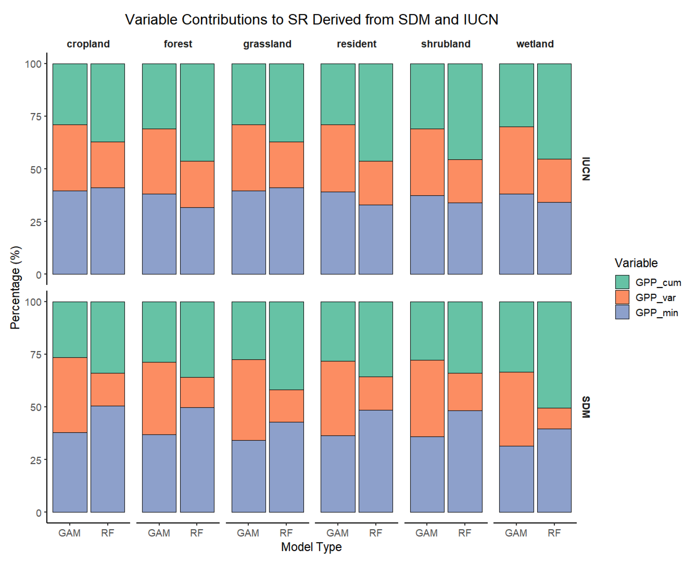
There were some differences in the relative contributions of the three DHI components to resident bird richness depending on whether SDM- or IUCN-based richness was used. DHIvar contributed more to the prediction of SDM-derived richness, whereas DHIcum accounted for a larger proportion of the explained variance for IUCN range map richness (Figure 5). Nevertheless, both richness sources showed a common pattern: Minimum DHI generally made the smallest contribution, a trend that was particularly evident in the GLMs and RF model. For the same richness source, model performance also varied between different models. In GAMs, the variance explained by the three DHI components was more evenly distributed, in contrast to the greater disparity in variable importance observed in the other two modelling approaches.
Figure 5.
Relative importance of DHI components in models predicting overall and guild-specific resident bird richness. In panels (b–d), values on the vertical axis are analogous to bar heights in panel (a), to highlight consistency and variance in DHI contribution across guilds. For individual guild-specific plots in the same format as panel (a), see Figure A4.
We assessed variable importance for the “All” predictor set across habitat guilds and summarized the results by group. The results revealed differences across data sources, modelling approaches, and variables. The predictive contribution of DHIs to richness showed a systematic difference between the two data sources. As shown in the figure, for the IUCN-based models, Cumulative DHI and Minimum DHI generally played dominant roles, with their variable importance accounting for a larger proportion of the explained variance in most habitats (cropland, forest, grassland, shrubland) and across both GLM and RF models, compared to their importance in SDM-based richness models. In contrast, for SDM-based models, Variation DHI was generally the most important predictor, contributing more to the richness of resident birds in cropland, forest, grassland, and shrubland than it did for IUCN-based richness, and this pattern was consistent across different modelling approaches. In addition, the two richness sources showed differing sensitivities to DHIs: when comparing across the five guilds, the importance of each DHI component was more variable (i.e., showed greater dispersion) in the SDM-based models than in the IUCN-based models, suggesting a higher sensitivity to environmental heterogeneity in SDM-based richness.
Resident birds in different habitat types exhibited varying dependencies on the three DHI components in the modelling process. For example, Cumulative DHI generally made a higher contribution to richness in forest and wetland guilds, while Variation DHI contributed least to wetland bird richness. The importance of Minimum DHI was relatively consistent across multiple habitat types, particularly for IUCN-based richness. In terms of the proportion of variable importance, the two nonlinear models showed clear differences. Random forest and GLM produced similar patterns and trends in variable importance across habitats, whereas the importance proportions in GAM were nearly the opposite for Cumulative DHI and Variation DHI compared to RF/GLM. Additionally, GAM tended to assign a more balanced contribution to each predictor variable, while in RF and GLM, the contributions of the DHI components were more disparate—a pattern consistently observed across all models.
4. Discussion
Our results support the use of DHIs as productivity-based predictors of resident bird richness patterns across China. This study included a comparative analysis of DHIs derived from different vegetation products, examined the correlations between DHIs and SDM-based resident bird richness, and validated the findings using IUCN range map-based richness. The comparative performance of three modelling approaches—GLM, GAM, and RF—suggests that Random Forests are particularly well suited for predicting richness from DHIs. The findings indicate that all three DHI components are moderately to highly correlated with resident bird richness: Cumulative DHI and Minimum DHI showed positive correlations, while Variation DHI was negatively correlated with richness. Among the vegetation products, GPP-derived DHIs showed the strongest associations with resident bird richness, indicating that DHIs can capture broad-scale richness gradients across habitat types, although productivity-based proxies may not fully reflect biodiversity variation in all contexts.
Climatic zonation and the associated energy–water constraints play a crucial role in shaping large-scale biodiversity gradients, and they also influence how the relationship between DHI and species richness should be interpreted. Because the DHI components primarily describe vegetation productivity and its temporal dynamics, DHI provides particularly useful information when resident bird richness is closely linked to ecosystem functioning. For instance, in energy-limited environments (e.g., high-elevation or cold regions), productivity-related signals often reflect constraints imposed by temperature and the length of the growing season; whereas in water-limited environments (e.g., arid and semi-arid regions), productivity and seasonality are more strongly governed by precipitation variability and drought stress. These contrasting climatic controls imply that the same DHI value may correspond to different habitat conditions across climate zones, highlighting the importance of explicitly considering climatic gradients when using DHI as a proxy for biodiversity.
We found a clear nonlinear relationship between DHIs and avian species richness. Stratified analyses further showed that the effects of DHIs vary across habitats, suggesting that available energy, environmental stability, and environmental stress jointly drive richness patterns.
Using single DHI components as predictors highlighted their differential influence across habitat guilds. Notably, models using Minimum DHI as the sole predictor achieved the highest adjusted R2, rather than those using Cumulative DHI, and this pattern was more pronounced in nonlinear models. This trend was also evident in IUCN-based modelling. For SDM richness, both RF and GAMs found that, except for wetland resident birds, Variation DHI models had adjusted R2 values second only to Minimum DHI, while Cumulative DHI models performed the worst; this pattern was not observed in GLM models. A similar trend was found for IUCN richness in RF/GAM models, although the difference in adjusted R2 between Variation DHI and Minimum DHI was small or negligible. In GLM models, Cumulative DHI was slightly lower than Minimum DHI but higher than Variation DHI.
In terms of variable importance, when all three DHI components were included simultaneously as predictors, both the cumulative DHI and the variation DHI emerged as key contributors to modelling resident bird richness in China. The prominent role of the cumulative DHI, which reflects annual cumulative available energy, is consistent with previous studies reporting strong energy–diversity linkages and the predictive value of cumulative productivity metrics for bird richness patterns. Our results further complement findings from tropical regions [66] by showing that the variation DHI can also play an important role when analyses span multiple climatic zones with pronounced seasonal contrasts. In tropical environments, intra-annual productivity fluctuations are often relatively modest, which may reduce the apparent contribution of variation-related metrics; however, across China’s broad climatic gradients, the variation DHI, capturing intra-annual fluctuations in productivity, provides additional explanatory power for resident birds that rely on local resources throughout the year [109]. Across habitat guilds, the cumulative DHI and variation DHI generally contributed more for cropland, forest, and shrubland birds, whereas the variation DHI tended to be less important for wetland birds. By contrast, the minimum DHI showed a relatively smaller overall contribution to explaining resident bird richness.
At the national scale, DHIs capture three dimensions—annual available energy, environmental stress, and environmental stability—each of which influences species richness through both correlated and complementary effects. Consequently, including all three components in a single model enables the capture of more information, resulting in higher model fit compared to using any single DHI component alone. This complementarity has been demonstrated globally, with DHIs explaining 67%, 65%, and 61% of the variation in amphibian, resident bird, and mammal species richness, respectively, and showing significant correlations [61]. When using only DHIcum as a predictor, the adjusted R2 is relatively low. However, when all three DHIs are combined in the model, the variable importance of DHIcum is enhanced. One possible reason for this is that, in single-component models, each DHI component contains shared variance with the other two, due to inter-component correlations. The improvement in adjusted R2 in the combined model arises from both the independent contributions of each DHI component and the shared variance among them. In multivariate models, this shared variance is redistributed, making the independent effects of each component more reliable [110,111]. This also explains why, in single-variable settings, DHImin reflects not only minimum productivity as an indicator of environmental stress, but also acts partly as a proxy for the available energy gradient. When modelled jointly, the explanatory power shared by DHImin and DHIcum is reallocated to DHIcum. Thus, this pattern does not contradict previous findings from global and other national-scale studies.
The relatively low importance of Variation DHI for wetland resident birds may be explained by the fact that seasonal fluctuations in wetland productivity are primarily governed by hydrological processes rather than vegetation phenology. In wetlands such as floodplains, lateral exchange caused by periodic changes in water levels shapes the moving littoral zone in the aquatic/terrestrial transition zone (ATTZ), which largely determines the spatiotemporal patterns of available habitat and productivity [112,113,114]. Different water level zones influence the area and connectivity of shallow water and emergent vegetation habitats, which in turn affect birds’ ability to utilize spatial resources such as foraging windows [115]. For example, the number of nests built by Ardeidae species is regulated by the number of days suitable habitat is available; changes in wader communities are attributed to water level trajectories; and the breeding season of Fulica atra is affected by the periodicity of water level fluctuations [116,117,118]. For resident birds, under certain extreme conditions, when habitat productivity declines below a critical level (e.g., affecting overwinter survival or creating seasonal bottlenecks), environmental stress may exert a stronger influence on richness than cumulative productivity. However, we consider this result should be interpreted with caution. We note that modelling richness using a single DHI component alone makes it difficult to determine the relative ordering of contributions among components. Therefore, we further examined model importance by including all variables within the same model and quantifying their contributions to assess their relative explanatory power.
From a technical perspective, medium-resolution satellite imagery has limited ability to capture the mosaic of open water, mudflats, and shallow water zones, with small-scale environmental heterogeneity likely to be smoothed out. Moreover, satellite-derived gross primary productivity (GPP) estimates primarily reflect emergent and floating vegetation, and, to avoid interference from non-productive pixels, we only retained pixels with valid values in every monthly image, further limiting our ability to capture the effects of periodic water-level changes on some ATTZ areas. These factors likely weakened the correlation between Variation DHI and wetland resident bird richness. Therefore, modelling richness in wetland guilds may require the incorporation of additional dynamic hydrological variables, such as time series of water depth, to supplement DHIs in predicting wetland resident bird richness. The productivity resources generated by hydrological processes ultimately translate into available habitat, which is precisely what cumulative available energy represents in wetlands, thus explaining the particular importance of Cumulative DHI for wetland resident birds.
Our results did not show as strong an effect of Variation DHI on grassland resident birds as has been reported for tropical regions [66]. This likely reflects differences in climate: grasslands in China are mostly located in temperate, subarctic, or arctic climate zones, where increased intra-annual variability in precipitation and temperature during the growing season tends to reduce species asynchrony and overall richness. As a result, grassland communities become more sensitive to cumulative productivity and to periods of low productivity within the annual productivity curve [86]. For example, on the Mongolian Plateau, species richness is more strongly associated with Cumulative DHI [67].
The differences between SDM- and IUCN-based richness are mainly reflected in their responses to DHIs. We found that, when jointly predicting resident bird richness, both Cumulative DHI and Minimum DHI contributed more to IUCN-based richness stratified by habitat guild than to SDM-based richness, consistent with results for overall resident bird richness. Meanwhile, the contribution of Variation DHI to forest and shrubland guilds differed markedly between the two data sources; specifically, Variation DHI showed stronger associations with SDM-based richness for these guilds.
There are several potential reasons for this pattern. Firstly, SDM-derived habitat ranges represent the probability of species occurrence in the environment, and the use of citizen science datasets as input may introduce biases related to observation effort and periodicity [91,119,120]. Secondly, our models incorporated climate and topographic variables as predictors for richness, which effectively captured some aspects of environmental heterogeneity, thereby increasing the sensitivity of predictions to seasonal fluctuations [5,121]. In contrast, IUCN range maps are constructed based on published data, expert judgement, and long-term records, representing boundaries that are relatively sensitive to broad-scale climatic patterns, energy flows, and environmental pressures driven by extreme events and cumulative productivity at the regional scale. We consider that the relatively weaker fit between DHIs and SDM-based grassland bird richness may be related to two factors. First, grassland habitats are often influenced by human activities such as grazing and hay mowing, which can alter land use intensity and local habitat conditions. Second, species occurrence records in grassland regions are often relatively sparse, which may increase the risk of sampling bias. Together, these factors may reduce the apparent sensitivity of grassland richness to DHIs.
Moreover, IUCN range maps are coarser in grain compared to SDM-based richness, which likely leads to a smoothing of the effects of environmental heterogeneity and seasonality within pixels, reducing their statistical sensitivity. In addition, IUCN-based richness includes more species—over 30% more than SDM-based richness. In China, forests span multiple vertical vegetation gradients, ranging from cold-temperate coniferous forests in the north to tropical rainforests in the south. The former exhibit greater intra-annual variability in productivity curves and a clearer distinction between growing and non-growing seasons. Coupled with the greater sensitivity of SDM-based richness to Variation DHI, this explains the higher importance of Variation DHI for the forest and shrubland guilds in the SDMs.
We consider random forest (RF) models to be better suited for predicting resident bird richness patterns for two reasons. Firstly, RF consistently achieved higher adjusted R2 values than both GAM and GLM, indicating a strong ability to capture richness patterns. Secondly, the predictive mechanism of RF is closer to that of linear models, and models that more closely approximate linear assumptions generally offer greater interpretability and lower extrapolation risk [122,123]. In contrast, GAMs permit greater smoothing and more pronounced nonlinearity, which can make interpretation of variable effects more challenging. We therefore favor the use of modelling approaches with lower complexity—provided that model performance is adequate—so as to explain ecological phenomena with simpler models [123].
We believe that Dynamic Habitat Indices (DHIs) have great potential for biodiversity conservation, but also have limitations. First, scale effects may influence our analyses to some extent. Second, satellite-derived productivity is subject to uncertainties associated with cloudy seasons, compositing algorithms, and sensor inconsistencies, which may reduce the accuracy in representing heterogeneity and seasonal dynamics. In addition, although the two richness products used in this study show overall consistency, it should be noted that they have complementary but different sources of bias. All these issues need be addressed in future work. From an applied perspective, using a nationally consistent DHI framework provides a transparent and scalable layer to support conservation planning and evaluation, information can complement policy frameworks such as the National Park System and the Ecological Conservation Redline by enabling cross-regional comparison, prioritization, and long-term monitoring. Nevertheless, DHI does not capture all determinants of bird richness, and remote-sensing uncertainty may increase in complex terrain or sparsely vegetated landscapes. Therefore, DHI-based inference should be interpreted as a broad-scale proxy and, where possible, integrated with additional ecological and anthropogenic factors in practical applications.
In summary, DHIs derived from satellite remote sensing datasets effectively capture intra-annual energy dynamics of habitats at large spatial scales, encompassing information on available energy, environmental stability, and environmental stress. These indices can be robustly linked to the species richness of resident birds across different guilds in China’s terrestrial ecosystems. The combination of multiple DHI components provides strong explanatory power for richness patterns, offering evidence for a deeper understanding of large-scale biodiversity—particularly the formation and drivers of avian diversity patterns. Both SDM- and IUCN-based richness products demonstrated overall consistency and reliability, while also highlighting their respective strengths. As the need for habitat assessment and biodiversity monitoring grows at large scales, and tracking spatiotemporal changes in biodiversity patterns becomes increasingly important, the observed relationship between DHIs and resident bird richness supports the use of DHIs as an effective tool for monitoring and assessing species and habitat patterns.
5. Conclusions
(a) DHIs represent a powerful set of indicators for understanding biodiversity patterns, with both the Cumulative DHI and the Variation DHI emerging as key predictors of bird species richness.
(b) Nonlinear models achieve better fits to richness patterns, the process of variable fitting in RF is more similar to that in GLM and aligns more closely with ecological principles, making RF particularly suitable for modelling.
(c) Differences between SDM- and IUCN-based richness are mainly reflected in their sensitivity to seasonal fluctuations across habitats, especially for forest and shrubland birds. SDM-based richness is more responsive to seasonal variation, while IUCN-based richness is more sensitive to available energy and environmental stress. Both approaches have their respective strengths and are reliable tools for biodiversity research.
Supplementary Materials
The following supporting information can be downloaded at: https://www.mdpi.com/article/10.3390/rs18030493/s1.
Author Contributions
Conceptualization, H.W., Y.Z. and M.J.M.B.; methodology, H.D. and M.J.M.B.; software, H.D.; validation, L.L. and H.Z.; resources, H.W.; writing—original draft preparation, H.D.; writing—review and editing, H.D. and M.J.M.B.; visualization, K.X. and Y.Y.; supervision, M.J.M.B. and H.W.; project administration, H.W.; funding acquisition, H.W.; All authors have read and agreed to the published version of the manuscript.
Funding
This research was funded by the National Natural Science Foundation of China (grant number NSFC: 42011530175, 42301288) and the National Key Research and Development Program of China, grant number 2021YFB3901100.
Data Availability Statement
The raw data supporting the conclusions of this article will be made available by the authors on request.
Acknowledgments
The author greatly appreciate the constructive comments provided by the reviewers and the editor.
Conflicts of Interest
The authors declare no conflicts of interest.
Appendix A
Table A1.
Environmental variables.
Table A2.
Model performance under 5-fold spatial block cross-validation (200 km × 200 km blocks) for SDM-derived resident and forest resident bird richness in China (mean ± SD of R2 and RMSE across folds).
Figure A1.
Interannual variation in the spatial mean of GPP-based DHI components (DHIcum, DHIvar, and DHImin) across China from 2012 to 2023.
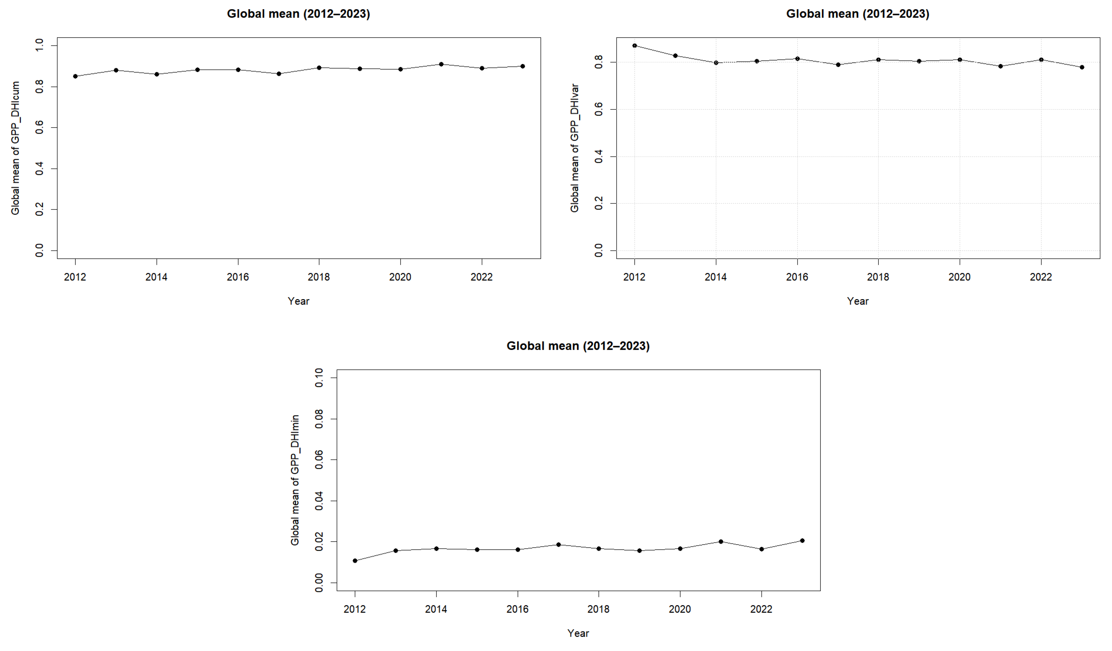
Figure A2.
Patterns of resident bird richness in China in SDMs.
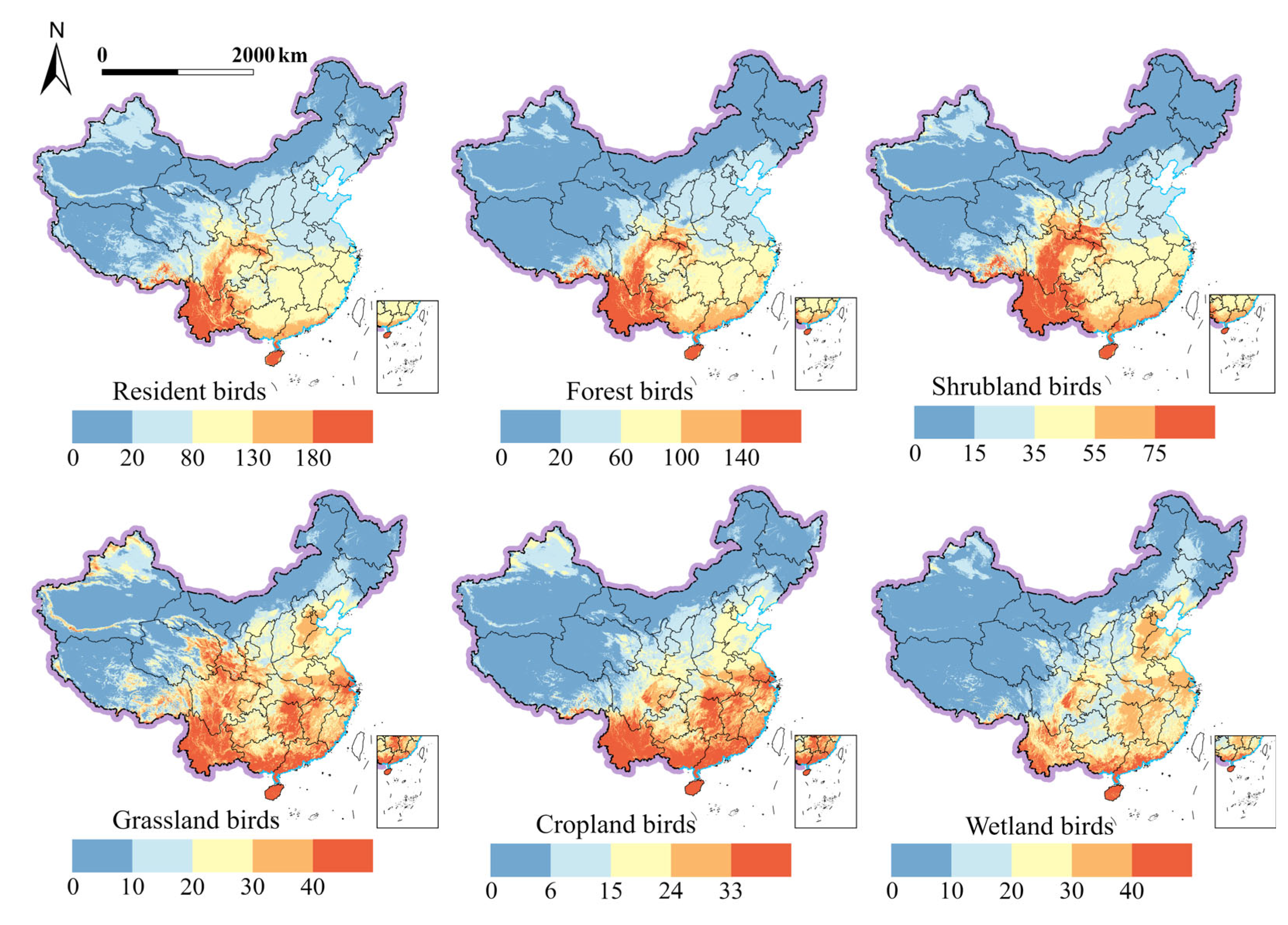
Figure A3.
Patterns of resident bird richness in China based on IUCN range maps.
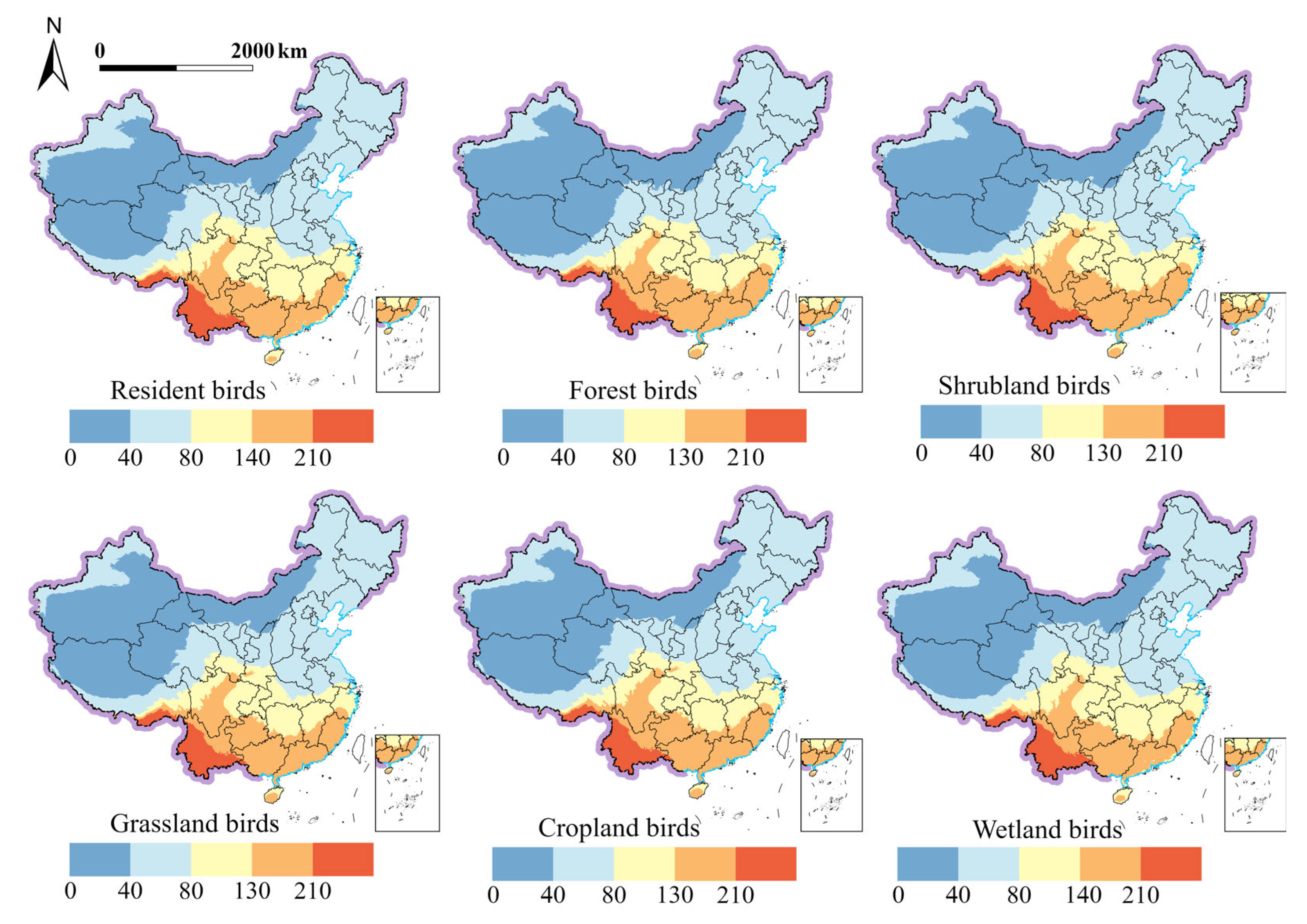
Figure A4.
Stacked bar chart of the relative importance of DHI components in models predicting all and guild-specific resident bird richness.
References
- Díaz, S.; Settele, J.; Brondízio, E.S.; Ngo, H.T.; Guèze, M.; Agard, J.; Arneth, A.; Balvanera, P.; Brauman, K.A.; Butchart, S.H.M.; et al. (Eds.) IPBES Summary for Policymakers of the Global Assessment Report on Biodiversity and Ecosystem Services of the Intergovernmental Science-Policy Platform on Biodiversity and Ecosystem Services; IPBES Secretariat: Bonn, Germany, 2019. [Google Scholar]
- Brauman, K.A.; Garibaldi, L.A.; Polasky, S.; Aumeeruddy-Thomas, Y.; Brancalion, P.H.S.; DeClerck, F.; Jacob, U.; Mastrangelo, M.E.; Nkongolo, N.V.; Palang, H.; et al. Global Trends in Nature’s Contributions to People. Proc. Natl. Acad. Sci. USA 2020, 117, 32799–32805. [Google Scholar] [CrossRef] [Scilit] [PubMed]
- Coelho, M.T.P.; Barreto, E.; Rangel, T.F.; Diniz-Filho, J.A.F.; Wüest, R.O.; Bach, W.; Skeels, A.; McFadden, I.R.; Roberts, D.W.; Pellissier, L.; et al. The Geography of Climate and the Global Patterns of Species Diversity. Nature 2023, 622, 537–544. [Google Scholar] [CrossRef] [Scilit] [PubMed]
- Pereira, H.M.; Martins, I.S.; Rosa, I.M.D.; Kim, H.; Leadley, P.; Popp, A.; Van Vuuren, D.P.; Hurtt, G.; Quoss, L.; Arneth, A.; et al. Global Trends and Scenarios for Terrestrial Biodiversity and Ecosystem Services from 1900 to 2050. Science 2024, 384, 458–465. [Google Scholar] [CrossRef] [Scilit] [PubMed]
- Elith, J.; Leathwick, J.R. Species Distribution Models: Ecological Explanation and Prediction Across Space and Time. Annu. Rev. Ecol. Evol. Syst. 2009, 40, 677–697. [Google Scholar] [CrossRef] [Scilit]
- Newbold, T.; Hudson, L.N.; Hill, S.L.L.; Contu, S.; Lysenko, I.; Senior, R.A.; Börger, L.; Bennett, D.J.; Choimes, A.; Collen, B.; et al. Global Effects of Land Use on Local Terrestrial Biodiversity. Nature 2015, 520, 45–50. [Google Scholar] [CrossRef] [Scilit]
- Blowes, S.A.; Supp, S.R.; Antão, L.H.; Bates, A.; Bruelheide, H.; Chase, J.M.; Moyes, F.; Magurran, A.; McGill, B.; Myers-Smith, I.H.; et al. The Geography of Biodiversity Change in Marine and Terrestrial Assemblages. Science 2019, 366, 339–345. [Google Scholar] [CrossRef] [Scilit]
- Williamson, M.; MacArthur, R.H. Geographical Ecology. Patterns in the Distribution of Species. J. Anim. Ecol. 1974, 43, 601. [Google Scholar] [CrossRef] [Scilit]
- Cooney, C.R.; Seddon, N.; Tobias, J.A. Widespread Correlations between Climatic Niche Evolution and Species Diversification in Birds. J. Anim. Ecol. 2016, 85, 869–878. [Google Scholar] [CrossRef] [Scilit]
- Buonincontri, M.P.; Bosso, L.; Smeraldo, S.; Chiusano, M.L.; Pasta, S.; Di Pasquale, G. Shedding Light on the Effects of Climate and Anthropogenic Pressures on the Disappearance of Fagus Sylvatica in the Italian Lowlands: Evidence from Archaeo-Anthracology and Spatial Analyses. Sci. Total Environ. 2023, 877, 162893. [Google Scholar] [CrossRef] [Scilit]
- Fraissinet, M.; Ancillotto, L.; Migliozzi, A.; Capasso, S.; Bosso, L.; Chamberlain, D.E.; Russo, D. Responses of Avian Assemblages to Spatiotemporal Landscape Dynamics in Urban Ecosystems. Landsc. Ecol. 2023, 38, 293–305. [Google Scholar] [CrossRef] [Scilit]
- Brown, J.H. Two Decades of Homage to Santa Rosalia: Toward a General Theory of Diversity. Am. Zool. 1981, 21, 877–888. [Google Scholar] [CrossRef] [Scilit]
- Wright, D.H. Species-Energy Theory: An Extension of Species-Area Theory. Oikos 1983, 41, 496. [Google Scholar] [CrossRef] [Scilit]
- Currie, D.J. Energy and Large-Scale Patterns of Animal- and Plant-Species Richness. Am. Nat. 1991, 137, 27–49. [Google Scholar] [CrossRef] [Scilit]
- Field, R.; Hawkins, B.A.; Cornell, H.V.; Currie, D.J.; Diniz-Filho, J.A.F.; Guégan, J.; Kaufman, D.M.; Kerr, J.T.; Mittelbach, G.G.; Oberdorff, T.; et al. Spatial Species-Richness Gradients across Scales: A Meta-Analysis. J. Biogeogr. 2009, 36, 132–147. [Google Scholar] [CrossRef] [Scilit]
- Hawkins, B.A.; Field, R.; Cornell, H.V.; Currie, D.J.; Guégan, J.-F.; Kaufman, D.M.; Kerr, J.T.; Mittelbach, G.G.; Oberdorff, T.; O’Brien, E.M.; et al. Energy, Water, and Broad-Scale Geographic Patterns of Species Richness. Ecology 2003, 84, 3105–3117. [Google Scholar] [CrossRef] [Scilit]
- Currie, D.J.; Mittelbach, G.G.; Cornell, H.V.; Field, R.; Guégan, J.; Hawkins, B.A.; Kaufman, D.M.; Kerr, J.T.; Oberdorff, T.; O’Brien, E.; et al. Predictions and Tests of Climate-based Hypotheses of Broad-scale Variation in Taxonomic Richness. Ecol. Lett. 2004, 7, 1121–1134. [Google Scholar] [CrossRef] [Scilit]
- O’Brien, E.M. Biological Relativity to Water–Energy Dynamics. J. Biogeogr. 2006, 33, 1868–1888. [Google Scholar] [CrossRef] [Scilit]
- Fuhrman, J.A.; Steele, J.A.; Hewson, I.; Schwalbach, M.S.; Brown, M.V.; Green, J.L.; Brown, J.H. A Latitudinal Diversity Gradient in Planktonic Marine Bacteria. Proc. Natl. Acad. Sci. USA 2008, 105, 7774–7778. [Google Scholar] [CrossRef] [Scilit]
- Pettorelli, N.; Safi, K.; Turner, W. Satellite Remote Sensing, Biodiversity Research and Conservation of the Future. Philos. Trans. R. Soc. B Biol. Sci. 2014, 369, 20130190. [Google Scholar] [CrossRef] [Scilit]
- Pettorelli, N.; Schulte To Bühne, H.; Tulloch, A.; Dubois, G.; Macinnis-Ng, C.; Queirós, A.M.; Keith, D.A.; Wegmann, M.; Schrodt, F.; Stellmes, M.; et al. Satellite Remote Sensing of Ecosystem Functions: Opportunities, Challenges and Way Forward. Remote Sens. Ecol. Conserv. 2018, 4, 71–93. [Google Scholar] [CrossRef] [Scilit]
- Skidmore, A.K.; Coops, N.C.; Neinavaz, E.; Ali, A.; Schaepman, M.E.; Paganini, M.; Kissling, W.D.; Vihervaara, P.; Darvishzadeh, R.; Feilhauer, H.; et al. Priority List of Biodiversity Metrics to Observe from Space. Nat. Ecol. Evol. 2021, 5, 896–906. [Google Scholar] [CrossRef] [Scilit] [PubMed]
- Turner, W.; Spector, S.; Gardiner, N.; Fladeland, M.; Sterling, E.; Steininger, M. Remote Sensing for Biodiversity Science and Conservation. Trends Ecol. Evol. 2003, 18, 306–314. [Google Scholar] [CrossRef] [Scilit]
- Tucker, C.J. Red and Photographic Infrared Linear Combinations for Monitoring Vegetation. Remote Sens. Environ. 1979, 8, 127–150. [Google Scholar] [CrossRef] [Scilit]
- Kaufman, Y.J.; Tanre, D. Atmospherically Resistant Vegetation Index (ARVI) for EOS-MODIS. IEEE Trans. Geosci. Remote Sens. 1992, 30, 261–270. [Google Scholar] [CrossRef] [Scilit]
- Hurlbert, A.H.; Haskell, J.P. The Effect of Energy and Seasonality on Avian Species Richness and Community Composition. Am. Nat. 2003, 161, 83–97. [Google Scholar] [CrossRef]
- Pettorelli, N.; Vik, J.O.; Mysterud, A.; Gaillard, J.-M.; Tucker, C.J.; Stenseth, N.C. Using the Satellite-Derived NDVI to Assess Ecological Responses to Environmental Change. Trends Ecol. Evol. 2005, 20, 503–510. [Google Scholar] [CrossRef] [Scilit]
- Krishnaswamy, J.; Bawa, K.S.; Ganeshaiah, K.N.; Kiran, M.C. Quantifying and Mapping Biodiversity and Ecosystem Services: Utility of a Multi-Season NDVI Based Mahalanobis Distance Surrogate. Remote Sens. Environ. 2009, 113, 857–867. [Google Scholar] [CrossRef] [Scilit]
- Huete, A.; Didan, K.; Miura, T.; Rodriguez, E.P.; Gao, X.; Ferreira, L.G. Overview of the Radiometric and Biophysical Performance of the MODIS Vegetation Indices. Remote Sens. Environ. 2002, 83, 195–213. [Google Scholar] [CrossRef] [Scilit]
- Camps-Valls, G.; Campos-Taberner, M.; Moreno-Martínez, Á.; Walther, S.; Duveiller, G.; Cescatti, A.; Mahecha, M.D.; Muñoz-Marí, J.; García-Haro, F.J.; Guanter, L.; et al. A Unified Vegetation Index for Quantifying the Terrestrial Biosphere. Sci. Adv. 2021, 7, eabc7447. [Google Scholar] [CrossRef] [Scilit]
- Knyazikhin, Y.; Martonchik, J.V.; Myneni, R.B.; Diner, D.J.; Running, S.W. Synergistic Algorithm for Estimating Vegetation Canopy Leaf Area Index and Fraction of Absorbed Photosynthetically Active Radiation from MODIS and MISR Data. J. Geophys. Res. Atmos. 1998, 103, 32257–32275. [Google Scholar] [CrossRef] [Scilit]
- Myneni, R.B.; Hoffman, S.; Knyazikhin, Y.; Privette, J.L.; Glassy, J.; Tian, Y.; Wang, Y.; Song, X.; Zhang, Y.; Smith, G.R.; et al. Global Products of Vegetation Leaf Area and Fraction Absorbed PAR from Year One of MODIS Data. Remote Sens. Environ. 2002, 83, 214–231. [Google Scholar] [CrossRef] [Scilit]
- Gitelson, A.A.; Peng, Y.; Huemmrich, K.F. Relationship between Fraction of Radiation Absorbed by Photosynthesizing Maize and Soybean Canopies and NDVI from Remotely Sensed Data Taken at Close Range and from MODIS 250 m Resolution Data. Remote Sens. Environ. 2014, 147, 108–120. [Google Scholar] [CrossRef] [Scilit]
- Monteith, J.L. Climate and the Efficiency of Crop Production in Britain. Phil. Trans. R. Soc. Lond. B 1977, 281, 277–294. [Google Scholar] [CrossRef] [Scilit]
- Running, S.W.; Nemani, R.R.; Heinsch, F.A.; Zhao, M.; Reeves, M.; Hashimoto, H. A Continuous Satellite-Derived Measure of Global Terrestrial Primary Production. Bioscience 2004, 54, 547. [Google Scholar] [CrossRef] [Scilit]
- Beer, C.; Reichstein, M.; Tomelleri, E.; Ciais, P.; Jung, M.; Carvalhais, N.; Rödenbeck, C.; Arain, M.A.; Baldocchi, D.; Bonan, G.B.; et al. Terrestrial Gross Carbon Dioxide Uptake: Global Distribution and Covariation with Climate. Science 2010, 329, 834–838. [Google Scholar] [CrossRef] [Scilit]
- Wagle, P.; Xiao, X.; Torn, M.S.; Cook, D.R.; Matamala, R.; Fischer, M.L.; Jin, C.; Dong, J.; Biradar, C. Sensitivity of Vegetation Indices and Gross Primary Production of Tallgrass Prairie to Severe Drought. Remote Sens. Environ. 2014, 152, 1–14. [Google Scholar] [CrossRef] [Scilit]
- Huang, X.; Xiao, J.; Ma, M. Evaluating the Performance of Satellite-Derived Vegetation Indices for Estimating Gross Primary Productivity Using FLUXNET Observations across the Globe. Remote Sens. 2019, 11, 1823. [Google Scholar] [CrossRef] [Scilit]
- Guisan, A.; Zimmermann, N.E. Predictive Habitat Distribution Models in Ecology. Ecol. Model. 2000, 135, 147–186. [Google Scholar] [CrossRef] [Scilit]
- Guisan, A.; Thuiller, W. Predicting Species Distribution: Offering More than Simple Habitat Models. Ecol. Lett. 2005, 8, 993–1009. [Google Scholar] [CrossRef] [Scilit]
- Wilson, A.M.; Jetz, W. Remotely Sensed High-Resolution Global Cloud Dynamics for Predicting Ecosystem and Biodiversity Distributions. PLoS Biol. 2016, 14, e1002415. [Google Scholar] [CrossRef] [Scilit]
- Randin, C.F.; Ashcroft, M.B.; Bolliger, J.; Cavender-Bares, J.; Coops, N.C.; Dullinger, S.; Dirnböck, T.; Eckert, S.; Ellis, E.; Fernández, N.; et al. Monitoring Biodiversity in the Anthropocene Using Remote Sensing in Species Distribution Models. Remote Sens. Environ. 2020, 239, 111626. [Google Scholar] [CrossRef] [Scilit]
- Cavender-Bares, J.; Schneider, F.D.; Santos, M.J.; Armstrong, A.; Carnaval, A.; Dahlin, K.M.; Fatoyinbo, L.; Hurtt, G.C.; Schimel, D.; Townsend, P.A.; et al. Integrating Remote Sensing with Ecology and Evolution to Advance Biodiversity Conservation. Nat. Ecol. Evol. 2022, 6, 506–519. [Google Scholar] [CrossRef] [Scilit] [PubMed]
- Timmermans, J.; Kissling, W. Advancing Terrestrial Biodiversity Monitoring with Satellite Remote Sensing in the Context of the Kunming-Montreal Global Biodiversity Framework. Ecol. Indic. 2023, 154, 110773. [Google Scholar] [CrossRef] [Scilit]
- Mittelbach, G.G.; Steiner, C.F.; Scheiner, S.M.; Gross, K.L.; Reynolds, H.L.; Waide, R.B.; Willig, M.R.; Dodson, S.I.; Gough, L. What Is the Observed Relationship Between Species Richness and Productivity? Ecology 2001, 82, 2381–2396. [Google Scholar] [CrossRef]
- Allen, A.P.; Brown, J.H.; Gillooly, J.F. Global Biodiversity, Biochemical Kinetics, and the Energetic-Equivalence Rule. Science 2002, 297, 1545–1548. [Google Scholar] [CrossRef] [Scilit]
- Evans, K.L.; Greenwood, J.J.D.; Gaston, K.J. Dissecting the Species–Energy Relationship. Proc. R. Soc. B Biol. Sci. 2005, 272, 2155–2163. [Google Scholar] [CrossRef] [Scilit]
- Rohde, K. Latitudinal Gradients in Species Diversity: The Search for the Primary Cause. Oikos 1992, 65, 514. [Google Scholar] [CrossRef] [Scilit]
- Tilman, D.; Reich, P.B.; Knops, J.M.H. Biodiversity and Ecosystem Stability in a Decade-Long Grassland Experiment. Nature 2006, 441, 629–632. [Google Scholar] [CrossRef] [Scilit]
- Wagg, C.; Roscher, C.; Weigelt, A.; Vogel, A.; Ebeling, A.; De Luca, E.; Roeder, A.; Kleinspehn, C.; Temperton, V.M.; Meyer, S.T.; et al. Biodiversity–Stability Relationships Strengthen over Time in a Long-Term Grassland Experiment. Nat. Commun. 2022, 13, 7752. [Google Scholar] [CrossRef] [Scilit]
- Hawkins, B.A.; Porter, E.E.; Felizola Diniz-Filho, J.A. Productivity and History as Predictors of the Latitudinal Diversity Gradient of Terrestrial Birds. Ecology 2003, 84, 1608–1623. [Google Scholar] [CrossRef] [Scilit]
- Coops, N.C.; Wulder, M.A.; Iwanicka, D. Exploring the Relative Importance of Satellite-Derived Descriptors of Production, Topography and Land Cover for Predicting Breeding Bird Species Richness over Ontario, Canada. Remote Sens. Environ. 2009, 113, 668–679. [Google Scholar] [CrossRef] [Scilit]
- Mackey, B.; Bryan, J.; Randall, L. Australia’s Dynamic Habitat Template 2003; The Australian National University: Canberra, Australia, 2004. [Google Scholar]
- Berry, S.; Mackey, B.; Brown, T. Potential Applications of Remotely Sensed Vegetation Greenness to Habitat Analysis and the Conservation of Dispersive Fauna. Pac. Conserv. Biol. 2007, 13, 120. [Google Scholar] [CrossRef] [Scilit]
- Coops, N.C.; Wulder, M.A.; Duro, D.C.; Han, T.; Berry, S. The Development of a Canadian Dynamic Habitat Index Using Multi-Temporal Satellite Estimates of Canopy Light Absorbance. Ecol. Indic. 2008, 8, 754–766. [Google Scholar] [CrossRef] [Scilit]
- Michaud, J.-S.; Coops, N.C.; Andrew, M.E.; Wulder, M.A. Characterising Spatiotemporal Environmental and Natural Variation Using a Dynamic Habitat Index throughout the Province of Ontario. Ecol. Indic. 2012, 18, 303–311. [Google Scholar] [CrossRef] [Scilit]
- Coops, N.C.; Wulder, M.A.; Iwanicka, D. Demonstration of a Satellite-Based Index to Monitor Habitat at Continental-Scales. Ecol. Indic. 2009, 9, 948–958. [Google Scholar] [CrossRef] [Scilit]
- Wang, Y.; Wu, W.; Guo, H.; Chen, Q.; Xu, H.; Xie, T.; Shi, Z. Spatiotemporal Variations and Correlation Factors of Species Habitat Appropriateness in China from a Satellite-Based Perspective. Ecol. Indic. 2023, 151, 110317. [Google Scholar] [CrossRef] [Scilit]
- Coops, N.C.; Kearney, S.P.; Bolton, D.K.; Radeloff, V.C. Remotely-Sensed Productivity Clusters Capture Global Biodiversity Patterns. Sci. Rep. 2018, 8, 16261. [Google Scholar] [CrossRef] [Scilit]
- Radeloff, V.C.; Dubinin, M.; Coops, N.C.; Allen, A.M.; Brooks, T.M.; Clayton, M.K.; Costa, G.C.; Graham, C.H.; Helmers, D.P.; Ives, A.R.; et al. The Dynamic Habitat Indices (DHIs) from MODIS and Global Biodiversity. Remote Sens. Environ. 2019, 222, 204–214. [Google Scholar] [CrossRef] [Scilit]
- Coops, N.C.; Bolton, D.K.; Hobi, M.L.; Radeloff, V.C. Untangling Multiple Species Richness Hypothesis Globally Using Remote Sensing Habitat Indices. Ecol. Indic. 2019, 107, 105567. [Google Scholar] [CrossRef] [Scilit]
- Coops, N.C.; Waring, R.H.; Wulder, M.A.; Pidgeon, A.M.; Radeloff, V.C. Bird Diversity: A Predictable Function of Satellite-derived Estimates of Seasonal Variation in Canopy Light Absorbance across the United States. J. Biogeogr. 2009, 36, 905–918. [Google Scholar] [CrossRef] [Scilit]
- Hobi, M.L.; Dubinin, M.; Graham, C.H.; Coops, N.C.; Clayton, M.K.; Pidgeon, A.M.; Radeloff, V.C. A Comparison of Dynamic Habitat Indices Derived from Different MODIS Products as Predictors of Avian Species Richness. Remote Sens. Environ. 2017, 195, 142–152. [Google Scholar] [CrossRef] [Scilit]
- Hobi, M.L.; Farwell, L.S.; Dubinin, M.; Kolesov, D.; Pidgeon, A.M.; Coops, N.C.; Radeloff, V.C. Patterns of Bird Species Richness Explained by Annual Variation in Remotely Sensed Dynamic Habitat Indices. Ecol. Indic. 2021, 127, 107774. [Google Scholar] [CrossRef] [Scilit]
- Zhang, C.; Li, L.; Guan, Y.; Cai, D.; Chen, H.; Bian, X.; Guo, S. Impacts of Vegetation Properties and Temperature Characteristics on Species Richness Patterns in Drylands: Case Study from Xinjiang. Ecol. Indic. 2021, 133, 108417. [Google Scholar] [CrossRef] [Scilit]
- Suttidate, N.; Hobi, M.L.; Pidgeon, A.M.; Round, P.D.; Coops, N.C.; Helmers, D.P.; Keuler, N.S.; Dubinin, M.; Bateman, B.L.; Radeloff, V.C. Tropical Bird Species Richness Is Strongly Associated with Patterns of Primary Productivity Captured by the Dynamic Habitat Indices. Remote Sens. Environ. 2019, 232, 111306. [Google Scholar] [CrossRef] [Scilit]
- Liu, Y.; Yang, Y.; Yue, X.; Chen, X.; Liu, Y. Dynamic Habitat Indices and Climatic Characteristics Explain Species Richness Patterns on the Mongolian Plateau. Remote Sens. 2023, 15, 1092. [Google Scholar] [CrossRef] [Scilit]
- Zhang, C.; Cai, D.; Guo, S.; Guan, Y.; Fraedrich, K.; Nie, Y.; Liu, X.; Bian, X. Spatial-Temporal Dynamics of China’s Terrestrial Biodiversity: A Dynamic Habitat Index Diagnostic. Remote Sens. 2016, 8, 227. [Google Scholar] [CrossRef] [Scilit]
- Andrew, M.E.; Wulder, M.A.; Coops, N.C.; Baillargeon, G. Beta-Diversity Gradients of Butterflies along Productivity Axes. Glob. Ecol. Biogeogr. 2012, 21, 352–364. [Google Scholar] [CrossRef] [Scilit]
- Michaud, J.-S.; Coops, N.C.; Andrew, M.E.; Wulder, M.A.; Brown, G.S.; Rickbeil, G.J.M. Estimating Moose (Alces alces) Occurrence and Abundance from Remotely Derived Environmental Indicators. Remote Sens. Environ. 2014, 152, 190–201. [Google Scholar] [CrossRef] [Scilit]
- Razenkova, E.; Radeloff, V.C.; Dubinin, M.; Bragina, E.V.; Allen, A.M.; Clayton, M.K.; Pidgeon, A.M.; Baskin, L.M.; Coops, N.C.; Hobi, M.L. Vegetation Productivity Summarized by the Dynamic Habitat Indices Explains Broad-Scale Patterns of Moose Abundance across Russia. Sci. Rep. 2020, 10, 836. [Google Scholar] [CrossRef] [Scilit]
- Zhi, X.; Du, H.; Zhang, M.; Long, Z.; Zhong, L.; Sun, X. Mapping the Habitat for the Moose Population in Northeast China by Combining Remote Sensing Products and Random Forests. Global Ecol. Conserv. 2022, 40, e02347. [Google Scholar] [CrossRef] [Scilit]
- Coops, N.C.; Michaud, J.-S.; Andrew, M.E.; Wulder, M.A. Comparison of a Regional-Level Habitat Index Derived from MERIS and MODIS Estimates of Canopy-Absorbed Photosynthetically Active Radiation. Remote Sens. Lett. 2011, 2, 327–336. [Google Scholar] [CrossRef] [Scilit]
- Liu, K.; Cao, C.; Gao, S.; Yang, W.; Ma, X. Bridging Satellite Productivity and Global Biodiversity: Unveiling Insights through Dynamic Habitat Indices. J. Remote Sens. 2025, 5, 0624. [Google Scholar] [CrossRef] [Scilit]
- Silveira, E.M.O.; Pidgeon, A.M.; Farwell, L.S.; Hobi, M.L.; Razenkova, E.; Zuckerberg, B.; Coops, N.C.; Radeloff, V.C. Multi-Grain Habitat Models That Combine Satellite Sensors with Different Resolutions Explain Bird Species Richness Patterns Best. Remote Sens. Environ. 2023, 295, 113661. [Google Scholar] [CrossRef] [Scilit]
- Razenkova, E.; Lewińska, K.E.; Anand, A.; Yin, H.; Farwell, L.S.; Pidgeon, A.M.; Hostert, P.; Coops, N.C.; Radeloff, V.C. Medium-Resolution Dynamic Habitat Indices from Landsat and Sentinel-2 Satellite Imagery. Ecol. Indic. 2025, 173, 113367. [Google Scholar] [CrossRef] [Scilit]
- Fialas, P.C.; Santini, L.; Russo, D.; Amorim, F.; Rebelo, H.; Novella-Fernandez, R.; Marques, F.; Domer, A.; Vella, A.; Martinoli, A.; et al. Changes in Community Composition and Functional Diversity of European Bats under Climate Change. Conserv. Biol. 2025, 39, e70025. [Google Scholar] [CrossRef] [Scilit]
- Thonis, A.; Akçakaya, H.R. Perils of Using Range Maps in Macroecological Models of Species Richness. J. Biogeogr. 2025, 52, e15072. [Google Scholar] [CrossRef] [Scilit]
- Soley-Guardia, M.; Alvarado-Serrano, D.F.; Anderson, R.P. Top Ten Hazards to Avoid When Modeling Species Distributions: A Didactic Guide of Assumptions, Problems, and Recommendations. Ecography 2024, 2024, e06852. [Google Scholar] [CrossRef] [Scilit]
- La Sorte, F.A.; Hawkins, B.A. Range Maps and Species Richness Patterns: Errors of Commission and Estimates of Uncertainty. Ecography 2007, 30, 649–662. [Google Scholar] [CrossRef] [Scilit]
- Mi, X.; Feng, G.; Hu, Y.; Zhang, J.; Chen, L.; Corlett, R.T.; Hughes, A.C.; Pimm, S.; Schmid, B.; Shi, S.; et al. The Global Significance of Biodiversity Science in China: An Overview. Natl. Sci. Rev. 2021, 8, nwab032. [Google Scholar] [CrossRef] [Scilit]
- Zheng, G. A Checklist on the Classification and Distribution of the Birds of China, 4th ed.; Geological Publishing House: Beijing, China, 2023. [Google Scholar]
- Zhang, Y.; Zhang, Z.; Dong, L.; Ding, P.; Ding, C.; Ma, Z.; Zheng, G. Assessment of Red List of Birds in China. Biodivers. Sci. 2016, 24, 568–577. [Google Scholar] [CrossRef] [Scilit]
- Liu, J.; Li, S.; Ouyang, Z.; Tam, C.; Chen, X. Ecological and Socioeconomic Effects of China’s Policies for Ecosystem Services. Proc. Natl. Acad. Sci. USA 2008, 105, 9477–9482. [Google Scholar] [CrossRef] [Scilit] [PubMed]
- Wang, X.; Xiao, X.; Qin, Y.; Dong, J.; Wu, J.; Li, B. Improved Maps of Surface Water Bodies, Large Dams, Reservoirs, and Lakes in China. Earth Syst. Sci. Data 2022, 14, 3757–3771. [Google Scholar] [CrossRef] [Scilit]
- Hochachka, W.M.; Ruiz-Gutierrez, V.; Johnston, A. Considerations for Fitting Occupancy Models to Data from eBird and Similar Volunteer-Collected Data. Ornithology 2023, 140, ukad035. [Google Scholar] [CrossRef] [Scilit]
- Lindenmayer, D.B.; Lane, P.; Foster, C.N.; Westgate, M.J.; Sato, C.; Ikin, K.; Crane, M.; Michael, D.; Florance, D.; Scheele, B.C. Do Migratory and Resident Birds Differ in Their Responses to Interacting Effects of Climate, Weather and Vegetation? Divers. Distrib. 2019, 25, 449–461. [Google Scholar] [CrossRef] [Scilit]
- IUCN Habitats Classification Scheme, version 3.1; IUCN: Gland, Switzerland, 2012.
- Lumbierres, M.; Dahal, P.R.; Di Marco, M.; Butchart, S.H.M.; Donald, P.F.; Rondinini, C. Translating Habitat Class to Land Cover to Map Area of Habitat of Terrestrial Vertebrates. Conserv. Biol. 2022, 36, e13851. [Google Scholar] [CrossRef] [Scilit]
- Jung, M.; Dahal, P.R.; Butchart, S.H.M.; Donald, P.F.; De Lamo, X.; Lesiv, M.; Kapos, V.; Rondinini, C.; Visconti, P. A Global Map of Terrestrial Habitat Types. Sci. Data 2020, 7, 256. [Google Scholar] [CrossRef] [Scilit]
- Johnston, A.; Hochachka, W.M.; Strimas-Mackey, M.E.; Ruiz Gutierrez, V.; Robinson, O.J.; Miller, E.T.; Auer, T.; Kelling, S.T.; Fink, D. Analytical Guidelines to Increase the Value of Community Science Data: An Example Using eBird Data to Estimate Species Distributions. Divers. Distrib. 2021, 27, 1265–1277. [Google Scholar] [CrossRef] [Scilit]
- Strimas-Mackey, M.; Hochachka, W.M.; Ruiz-Gutierrez, V.; Robinson, O.J.; Miller, E.T.; Auer, T.; Kelling, S.; Fink, D.; Johnston, A. Best Practices for Using eBird Data v1.0; Zenodo, 2020; Available online: https://zenodo.org/records/3620739 (accessed on 18 January 2026).
- Yang, W.; Ma, K.; Kreft, H. Geographical Sampling Bias in a Large Distributional Database and Its Effects on Species Richness–Environment Models. J. Biogeogr. 2013, 40, 1415–1426. [Google Scholar] [CrossRef] [Scilit]
- Phillips, S.J.; Dudík, M.; Schapire, R.E. A Maximum Entropy Approach to Species Distribution Modeling. In Proceedings of the Twenty-First International Conference on Machine Learning –ICML ’04; Association for Computing Machinery: New York, NY, USA, 2004; p. 83. [Google Scholar]
- Phillips, S. Maxnet: Fitting “Maxent” Species Distribution Models with “Glmnet”, version 0.1.4; CRAN: Wien, Austria, 2021. [Google Scholar]
- Bosso, L.; Fichera, G.; Mucedda, M.; Pidinchedda, E.; Veith, M.; Smeraldo, S.; De Pasquale, P.P.; Mori, E.; Ancillotto, L. Island Life and Interspecific Dynamics Influence Body Size, Distribution and Ecological Niche of Long-Eared Bats. J. Biogeogr. 2025, 53, e70071. [Google Scholar] [CrossRef] [Scilit]
- Yousefi, M.; Nicolaï, M.P.J.; Bosso, L.; Kafash, A.; Nezami, B.; Rastegar-Pouyani, E. Global Scale High-Resolution Habitat Suitability Modeling of Avifauna Providing Pollination Service (Sunbirds, Nectariniidae). Sci. Rep. 2025, 15, 9489. [Google Scholar] [CrossRef] [Scilit] [PubMed]
- Santos, D.P.; Silva, T.S.F.; De Assis Figueiredo, F.A.M.M. Climate Change May Increase Environmental Suitability of the Babassu Complex (Attalea Spp., Arecaceae). J. Biogeogr. 2025, 52, e70027. [Google Scholar] [CrossRef] [Scilit]
- Anderle, M.; Paniccia, C.; Brambilla, M.; Hilpold, A.; Volani, S.; Tasser, E.; Seeber, J.; Tappeiner, U. The Contribution of Landscape Features, Climate and Topography in Shaping Taxonomical and Functional Diversity of Avian Communities in a Heterogeneous Alpine Region. Oecologia 2022, 199, 499–512. [Google Scholar] [CrossRef] [Scilit] [PubMed]
- Kawamura, K.; Yamaura, Y.; Senzaki, M.; Ueta, M.; Nakamura, F. Seasonality in Spatial Distribution: Climate and Land Use Have Contrasting Effects on the Species Richness of Breeding and Wintering Birds. Ecol. Evol. 2019, 9, 7549–7561. [Google Scholar] [CrossRef] [Scilit]
- Lennon, J.J.; Greenwood, J.J.D.; Turner, J.R.G. Bird Diversity and Environmental Gradients in Britain: A Test of the Species–Energy Hypothesis. J. Anim. Ecol. 2000, 69, 581–598. [Google Scholar] [CrossRef] [Scilit]
- Harrell, F.E., Jr.; Dupont, C. Hmisc: Harrell Miscellaneous, version 5.2-5; CRAN: Wien, Austria, 2025. [Google Scholar]
- Naimi, B. Usdm: Uncertainty Analysis for Species Distribution Models, version 2.1-7; CRAN: Wien, Austria, 2023. [Google Scholar]
- Cutler, D.R.; Edwards, T.C.; Beard, K.H.; Cutler, A.; Hess, K.T.; Gibson, J.; Lawler, J.J. Random Forests for Classification in Ecology. Ecology 2007, 88, 2783–2792. [Google Scholar] [CrossRef] [Scilit]
- Wood, S.N. Generalized Additive Models: An Introduction with R, 2nd ed.; Chapman and Hall/CRC: New York, NY, USA, 2017. [Google Scholar]
- Zuur, A.F.; Ieno, E.N.; Walker, N.; Saveliev, A.A.; Smith, G.M. Mixed Effects Models and Extensions in Ecology with R; Statistics for Biology and Health; Springer: New York, NY, USA, 2009. [Google Scholar]
- Kuhn, M. Building Predictive Models in R Using the Caret Package. J. Stat. Softw. 2008, 28, 1–26. [Google Scholar] [CrossRef] [Scilit]
- Noonan, M.J.; Fagan, W.F.; Fleming, C.H. A Semi-Variance Approach to Visualising Phylogenetic Autocorrelation. Methods Ecol. Evol. 2022, 13, 396–406. [Google Scholar] [CrossRef] [Scilit]
- White, E.P.; Ernest, S.K.M.; Adler, P.B.; Hurlbert, A.H.; Lyons, S.K. Integrating Spatial and Temporal Approaches to Understanding Species Richness. Philos. Trans. R. Soc. B Biol. Sci. 2010, 365, 3633–3643. [Google Scholar] [CrossRef] [Scilit]
- Lai, J.; Zou, Y.; Zhang, J.; Peres-Neto, P.R. Generalizing Hierarchical and Variation Partitioning in Multiple Regression and Canonical Analyses Using the Rdacca. Hp R Package. Methods Ecol. Evol. 2022, 13, 782–788. [Google Scholar] [CrossRef] [Scilit]
- Peres-Neto, P.R.; Legendre, P.; Dray, S.; Borcard, D. Variation Partitioning of Species Data Matrices: Estimation and Comparison of Fractions. Ecology 2006, 87, 2614–2625. [Google Scholar] [CrossRef] [Scilit]
- Bayley, P.B. Understanding Large River-Floodplain Ecosystems: Significant Economic Advantages and Increased Biodiversity and Stability Would Result from Restoration of Impaired Systems. Bioscience 1995, 45, 153–158. [Google Scholar] [CrossRef] [Scilit]
- Poff, N.L.; Allan, J.D.; Bain, M.B.; Karr, J.R.; Prestegaard, K.L.; Richter, B.D.; Sparks, R.E.; Stromberg, J.C. The Natural Flow Regime. Bioscience 1997, 47, 769–784. [Google Scholar] [CrossRef] [Scilit]
- Teng, J.; Zhu, Y.; Duan, H.; Yu, X.; Xia, S.; Wang, R.; Yang, H. Linking Hydrological Connectivity and Waterbirds Habitat Suitability in Floodplain Wetlands: Implications for Wetland Management. Ecol. Indic. 2025, 176, 113663. [Google Scholar] [CrossRef] [Scilit]
- Schaffer-Smith, D.; Swenson, J.J.; Reiter, M.E.; Isola, J.E. Quantifying Shorebird Habitat in Managed Wetlands by Modeling Shallow Water Depth Dynamics. Ecol. Appl. 2018, 28, 1534–1545. [Google Scholar] [CrossRef] [Scilit]
- Essian, D.A.; Dorn, N.J.; Gawlik, D.E. Hydrologically-Mediated Resource Availability Regulates Annual Wading Bird Breeding in a Littoral Marsh. Ecol. Indic. 2025, 174, 113414. [Google Scholar] [CrossRef] [Scilit]
- Yu, F.; Zhai, J.; Huang, Z.; Chen, J.; Han, F.; Wang, L. The Impact of Poyang Lake Water Level Changes on the Landscape Pattern of Wintering Wading Bird Habitats. Global Ecol. Conserv. 2025, 58, e03453. [Google Scholar] [CrossRef] [Scilit]
- Zhang, W.; Liu, T.; Cheng, K.; Rummy, P. Declining Water Depth Delayed the Breeding Time of Fulica Atra, Not Human Disturbance. PLoS ONE 2018, 13, e0202684. [Google Scholar] [CrossRef] [Scilit]
- Altwegg, R.; Nichols, J.D. Occupancy Models for Citizen-Science Data. Methods Ecol. Evol. 2019, 10, 8–21. [Google Scholar] [CrossRef] [Scilit]
- Prasad, A.; Peters, M.; Pedlar, J.; Gougherty, A.; McKenney, D.; Mora, F.; Matthews, S.; McNulty, S.; López-Mata, L. Habitat and Migration Dynamics of North American Tree Species Under Climate Change. J. Biogeogr. 2025, 52, e15138. [Google Scholar] [CrossRef] [Scilit]
- Ahmad, S.; Wanghe, K.; Jialing, L.; Gonzalez, E.B.; Syms, C.; Strelnikov, I.I.; Bosso, L.; Mao, W. Climate-Driven Morphological Variation in Passerine Birds. Glob. Ecol. Biogeogr. 2025, 34, e70164. [Google Scholar] [CrossRef] [Scilit]
- Yates, K.L.; Bouchet, P.J.; Caley, M.J.; Mengersen, K.; Randin, C.F.; Parnell, S.; Fielding, A.H.; Bamford, A.J.; Ban, S.; Barbosa, A.M.; et al. Outstanding Challenges in the Transferability of Ecological Models. Trends Ecol. Evol. 2018, 33, 790–802. [Google Scholar] [CrossRef] [Scilit]
- Merow, C.; Smith, M.J.; Edwards, T.C.; Guisan, A.; McMahon, S.M.; Normand, S.; Thuiller, W.; Wüest, R.O.; Zimmermann, N.E.; Elith, J. What Do We Gain from Simplicity versus Complexity in Species Distribution Models? Ecography 2014, 37, 1267–1281. [Google Scholar] [CrossRef] [Scilit]
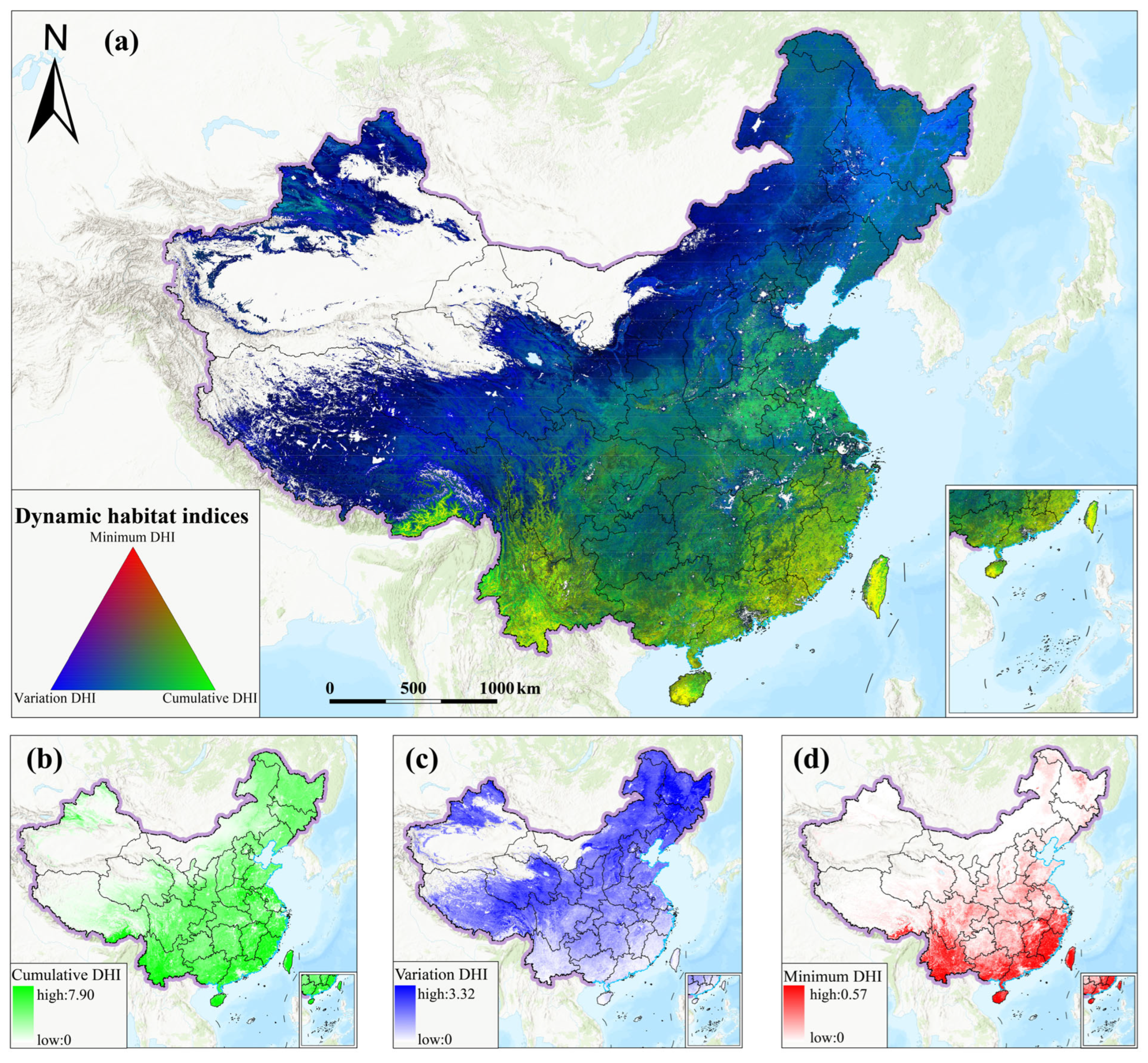
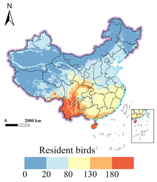
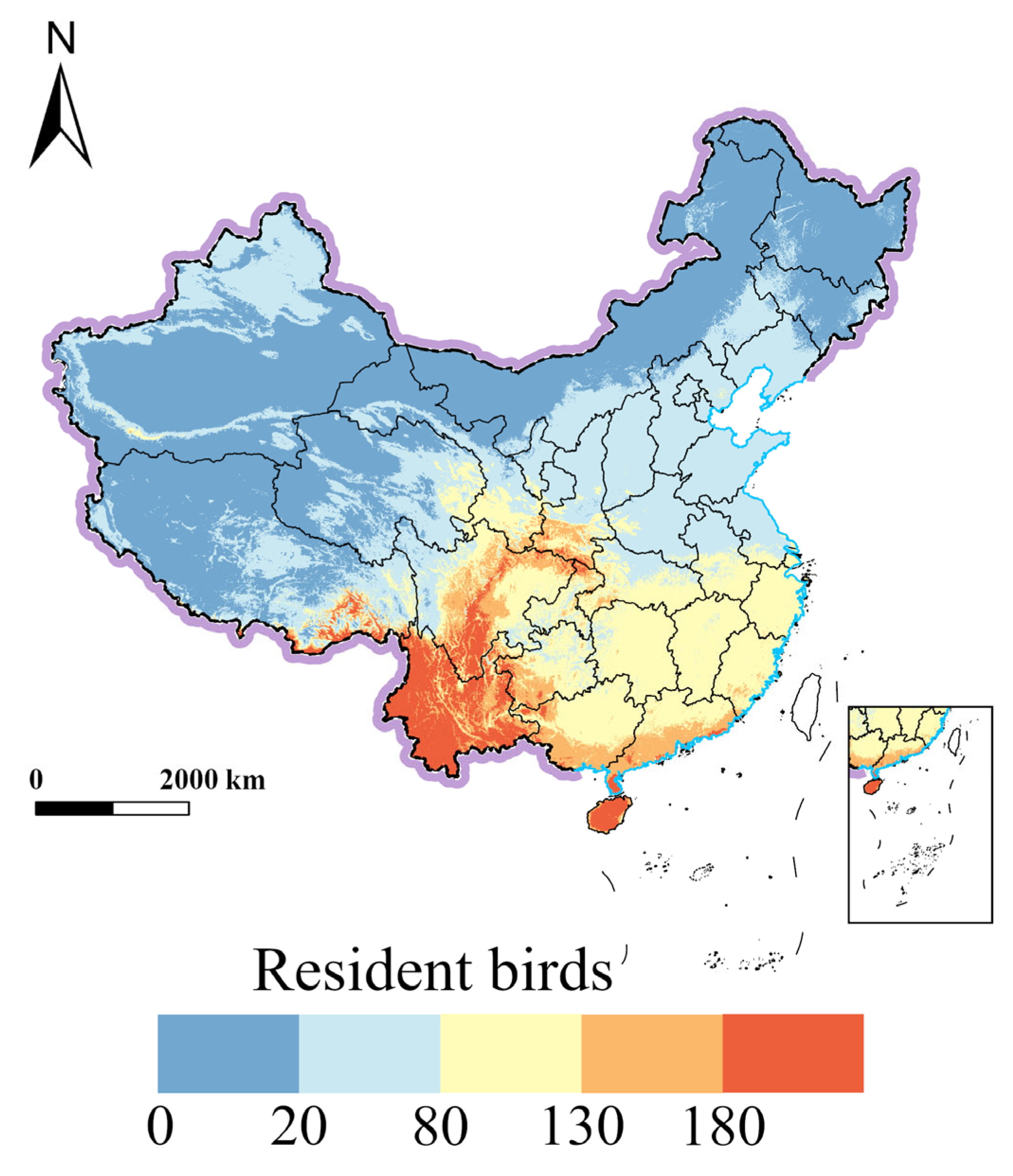
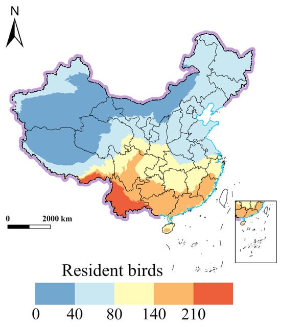
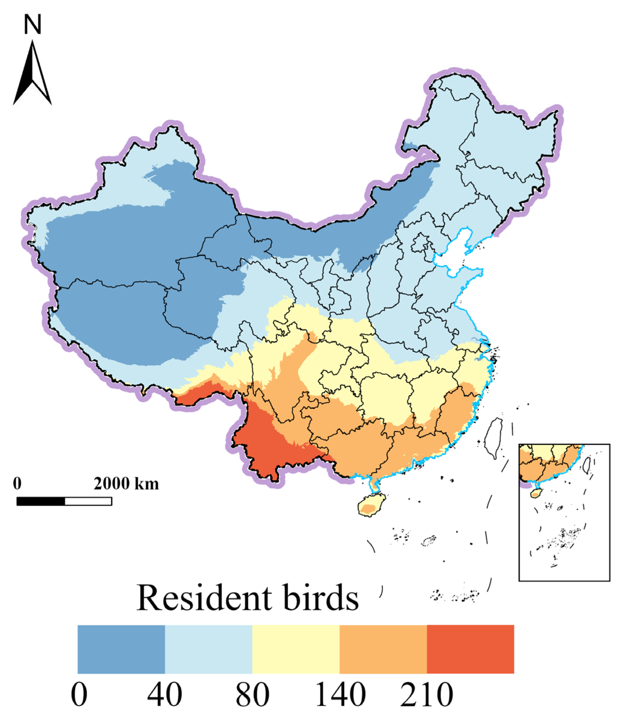
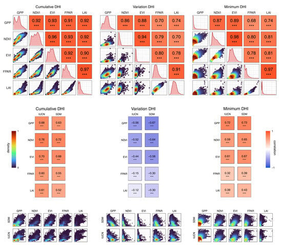
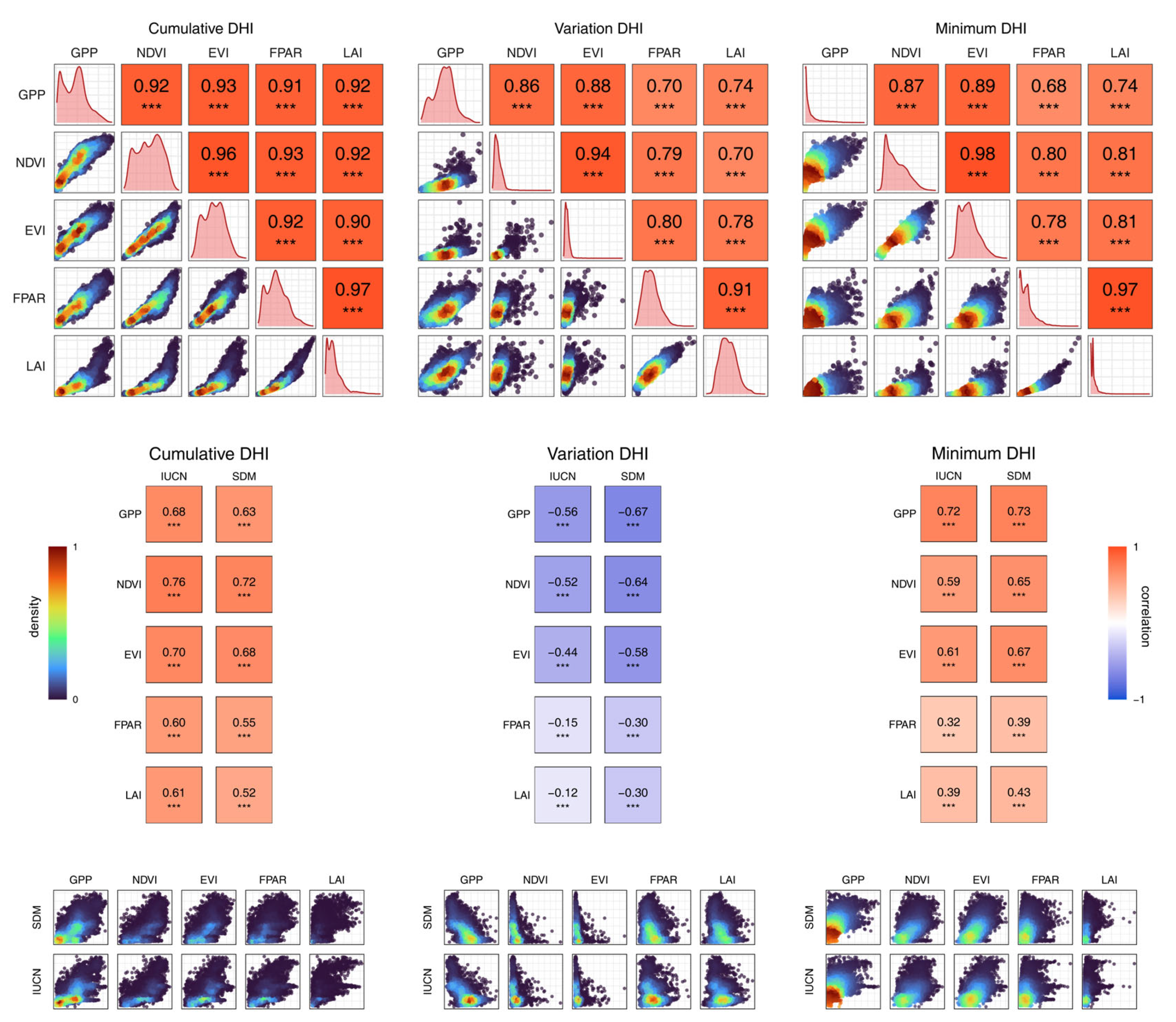
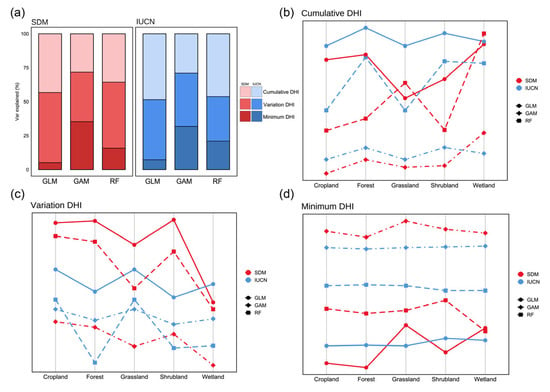
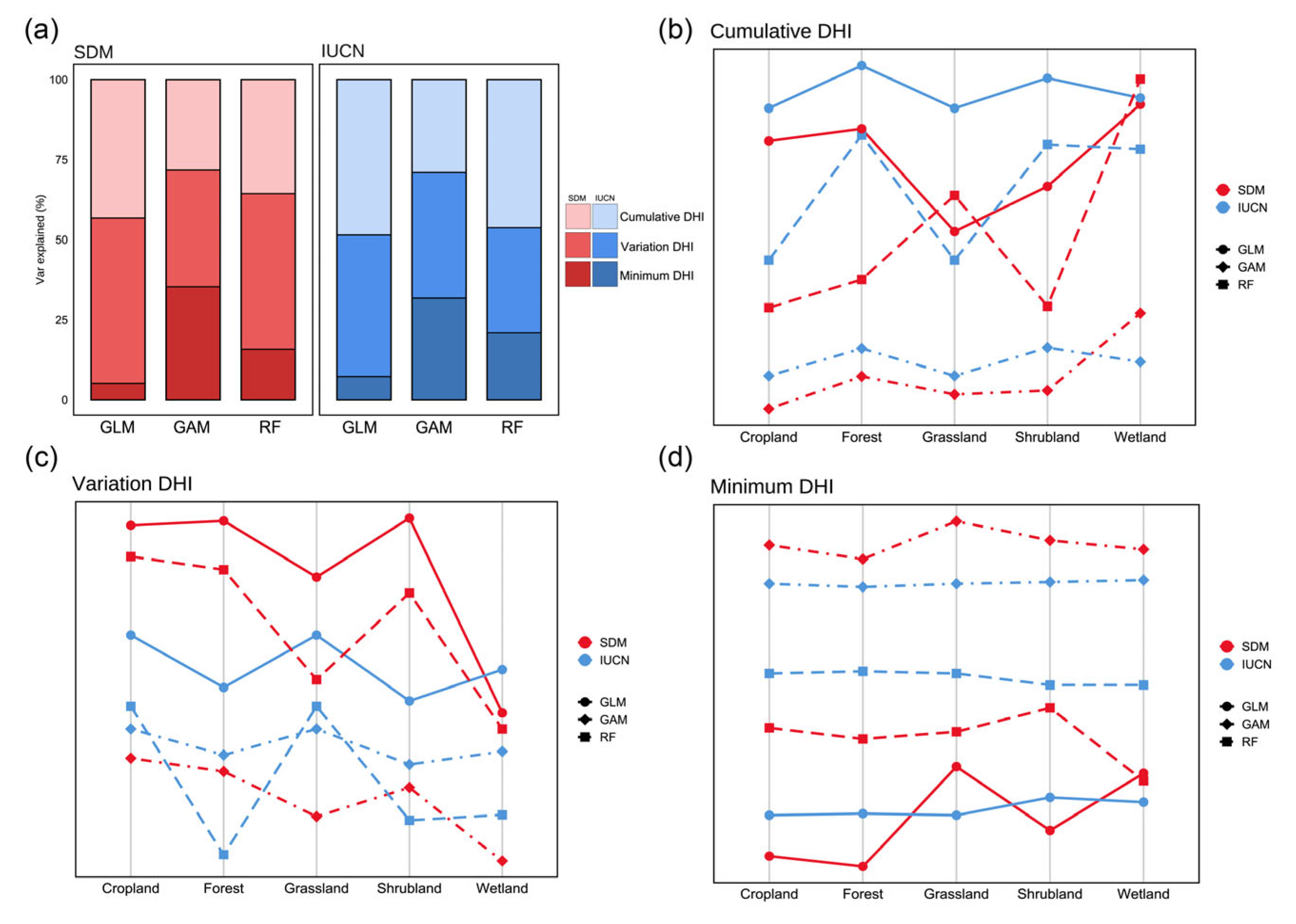

Disclaimer/Publisher’s Note: The statements, opinions and data contained in all publications are solely those of the individual author(s) and contributor(s) and not of MDPI and/or the editor(s). MDPI and/or the editor(s) disclaim responsibility for any injury to people or property resulting from any ideas, methods, instructions or products referred to in the content. |
© 2026 by the authors. Licensee MDPI, Basel, Switzerland. This article is an open access article distributed under the terms and conditions of the Creative Commons Attribution (CC BY) license.