


Highlights
What are the main findings?
- Relative to radar alone, adding the original optical input improves average mapped flood overlap and reduces flood-probability error in the evaluated systems.
- With reduced optical input, a small overlap gain can coexist with worse probabilities; permanent water accounts for much of this difference.
What are the implications of the main findings?
- Evaluate mapped flood extent and assigned flood probabilities separately before relying on an apparent fusion benefit.
- Single-event checks reveal transfer sensitivity and identify priorities for reference-time and multi-event evaluation.
Abstract
Adding optical imagery to radar can improve a flood map without improving the flood probabilities assigned to its pixels. We examine when these benefits agree, using a Sentinel-1 radar-only network as the reference for a Sentinel-1/Sentinel-2 fusion network. The same flood processes and reference pixels are compared as optical input is progressively masked. With no additional masking, fusion improves mean flood-area overlap by 0.0391/0.0373 and reduces mean flood-probability squared error by 0.0203/0.0211 on 18 internal and nine held-out flood episodes previously inspected during development. When only 25% of spatial blocks are retained, overlap gains remain slightly positive, but probability error increases by 0.0106/0.0091. Most of the original-optical probability benefit comes from avoiding false flood probabilities on reference permanent water; probability improvements on reference flood pixels are inconsistent. Controls and spatial examples expose trade-offs between missed floods and false floods. Additional single-event checks reveal adverse transfer. The practical contribution is evidence that flood-area accuracy and flood-probability quality must be assessed separately when optical support changes. This retrospective satellite-image assessment relates optical availability to flood-area accuracy and probability quality.
1. Introduction
Flood response requires maps before cloud-free optical imagery is necessarily available. Sentinel-1 (S1) radar can observe through clouds, whereas Sentinel-2 (S2) supplies complementary spectral information when acquisition timing and visibility permit. An archived S1/S2 pair nevertheless need not depict the same flood state. STURM-Flood documents the difficulty of obtaining useful paired observations [1], and ImpactMesh-Flood v1 provides a larger multi-temporal archive with Copernicus Emergency Management Service (CEMS)-derived labels [2]. Evaluating fusion, therefore, requires an explicit mapping time, a definition of valid optical support, and a clear statement of what the reference labels represent.
An equally important distinction concerns the output. A model can delineate flood extent better while assigning less accurate flood probabilities. An overall probability improvement can also originate mainly from pixels labeled permanent water rather than flood. Such differences matter when probability maps inform prioritization or subsequent analysis. We ask whether a fixed radar–optical system improves both flood segmentation and flood-probability quality relative to a radar-only reference as optical support decreases, and which reference classes account for the difference.
Flood early warning and satellite flood mapping both support flood response, but assess different outputs. Nearing et al. [3] evaluate forecasts of extreme river discharge in ungauged watersheds against the Global Flood Awareness System. Flood Hub makes flood forecasts accessible and also provides inundation information; its documentation distinguishes hydrologic and inundation-model evaluation [4]. Our study concerns pixel-level flood classification and assigned class probabilities from satellite images referenced to an S1 acquisition. Hydrological forecasting and satellite mapping use different targets, reference observations and evaluation scales. Their complementary roles motivate explicit assessment of both mapped extent and probability quality.
SAR-only flood mapping is well established through automated S1 processing [5], operational monitoring [6], and time-series approaches distinguishing unusual inundation from recurrent water [7]. S1/S2 comparisons and cross-benchmark studies show the importance of sensor choice, data curation and transfer [8,9]. SMAGNet already combines masked adaptive SAR–multispectral fusion with evaluation under added optical missingness [10]. CloudSeg and EarthMiss address incomplete optical inputs through other representation-learning strategies [11,12].
Probability assessment likewise has established foundations. Brier score measures squared probability error [13]; temperature scaling adjusts probabilities with one scalar [14] and probabilistic inundation studies already report Brier, logarithmic loss, calibration error and reliability diagrams [15]. A recent surface-water comparison separates configuration ranking from fixed-model input reliance, but uses an all-water target without inference-time optical input [16]. Our question concerns the flood class, its distinction from permanent water, and the agreement or disagreement of hard and probability outcomes under reduced pre-S1 optical support.
Reference definition and validation design constrain that question. Permanent-water information helps distinguish new inundation [17], a task evaluated using three-class references. Sen1Floods11 provides valuable manually checked water masks for the complementary binary evaluation [18]. Flood-map metrics also depend on class prevalence and sampling [19]. We, therefore, aggregate pixels within conservatively grouped flood processes, weight processes equally, and retain class-specific probability contributions. A process is a grouped flood episode, not an image tile or a training seed.
The main comparison is ordinary radar–optical fusion against radar alone, fitted on the same paired training pool and evaluated on the same reference pixels. Improvement means either greater overlap with the reference flood extent or smaller squared error of the assigned flood probabilities; these are separate outcomes. The contribution is to show, for the evaluated systems, when those improvements disagree as optical support declines, and to identify how permanent-water and flood pixels contribute to that disagreement. This extends assessment of fusion beyond a single segmentation ranking and gives users a concrete reason to examine the probability layer separately.
The main 18 internal and nine holdout processes had been inspected during earlier stages, so these comparisons remain retrospective. Controlled and external checks provide complementary sensitivity and transfer evidence. Favorable original-input means and adverse optical-loss, training and transfer outcomes are reported together.
2. Materials and Methods
The workflow has four steps. First, use the radar acquisition as the mapping-time anchor and select an eligible earlier optical image. Second, compare a radar-only map with a map produced from radar and optical inputs, using the same labeled locations. Third, progressively hide optical regions while leaving the radar image and reference locations unchanged. Fourth, ask separately whether mapped flood areas agree better with the reference and whether assigned flood probabilities have smaller errors. Flood intersection over union (IoU) measures the first outcome; flood Brier score measures the second. Higher IoU is better, whereas lower Brier is better. Each flood episode is summarized before episodes are averaged, preventing an episode with many image tiles from dominating. The details below make this comparison reproducible; Section 3.3 shows its spatial meaning for a real event.
2.1. Data, Mapping Time and Sample Roles
ImpactMesh-Flood v1 contains 24,578 tiles from 206 CEMS activations, including 19,448 official training tiles and a publisher-designated 562-tile holdout within its test split [2]. We use 256 × 256 S1 radiometrically terrain-corrected VV/VH, S2 Level-2A 12-band observations, and native labels: non-water (0), permanent water (1), flood (2), and Ignore (−1). The shared 10-m grid covers 2.56 × 2.56 km. The four archived time indices do not guarantee four synchronous sensor pairs. Event S1 index 2 defines the mapping anchor. JRC permanent-water information is not a model input.
A qualifying S2 acquisition precedes S1 by no more than 30 days and has at least 50% jointly valid pixels. Joint validity requires scene classes 4, 5 or 6, zero cloud and NaN masks, valid data mask, and all 12 bands finite and unequal to −9999. S1 must pass its data-mask and finite-value checks. Inputs and labels must agree in CRS, shape and pixel centers; labels and categorical masks use nearest-neighbor resampling if needed. Among eligible S2 candidates, we maximize valid area and break ties by recency. Training-role audits established these rules before formal fitting; evaluation does not relax them. We define optical age as and the signed offset as .
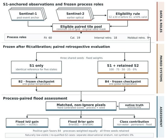
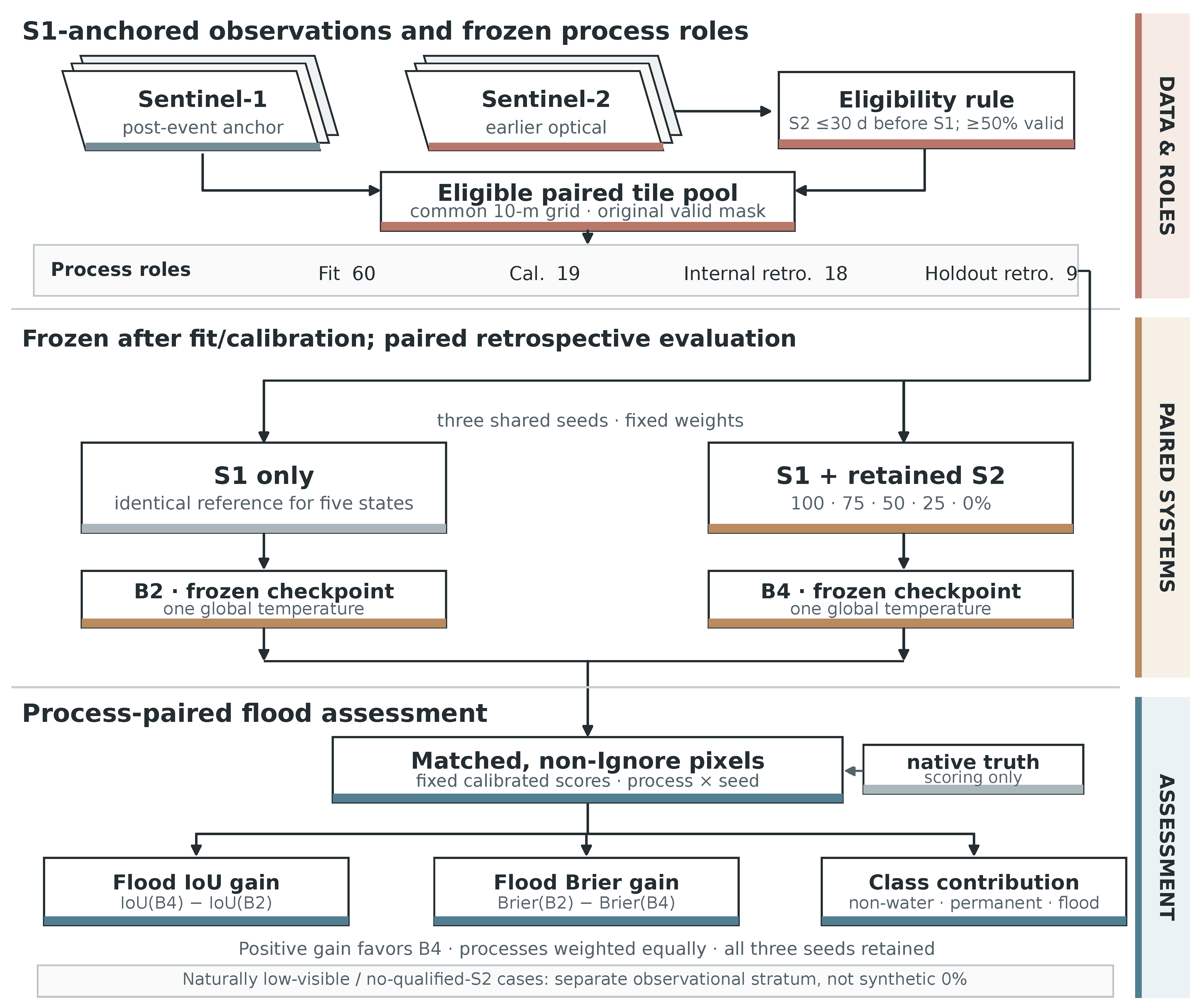
Sample construction first groups activations using public event evidence, then checks image eligibility, assigns complete grouped processes to roles, and removes duplicate scoring pixels. Official split names alone are insufficient because activations can span those splits. Earlier same-event discoveries involving Hurricane Irma and Storm Boris led to recorded safety exclusions before calibration/test-label inspection; these are dated amendments rather than the original preregistration. The later conservative spatial rule also excludes whole tiles with positive-area cross-role 10-m-grid overlap. The resulting role counts are given below (Figure 1); the manifests and historical population ledger are retained in Appendix A.1. Grouping and spatial checks address known event and spatial dependence.
Figure 1.
Design of the retrospective paired assessment. S1 anchors the mapping time; qualified earlier S2 is progressively masked while S1, checkpoints, scoring pixels and each model’s original global temperature remain fixed. The 60/19/18/9 role counts refer to the later three-seed analysis. Nested masks are schematic, not model predictions.
The paired analysis contains 3525 fit tiles from 60 grouped processes (66 activations), 2117 calibration tiles from 19 processes (20 activations), 1906 internal tiles from 18 processes (18 activations), and 432 holdout tiles from nine processes (nine activations). The fit role estimates weights and normalization; the separate calibration role estimates temperatures. Only the internal and holdout roles supply the paired result curves. Keeping these roles distinct is essential: thousands of tiles do not constitute thousands of independent flood events.
The 492 parent holdout tiles comprise 432 pairs, 49 tiles failing the visibility rule, and 11 without qualifying S2. The latter two are observational strata, spanning five and one process units, respectively; these counts can overlap the paired role and must not be added. They are not randomized missingness or proof that no optical image existed. The paired holdout’s median optical age is 19.03 days. The earlier formal timing summary reported 19.26 days on 430 eligible holdout tiles, excluding two tiles under its reporting rule; its internal median was 18.80 days. These describe different populations and indicate substantial asynchrony rather than contemporaneous flood observations.
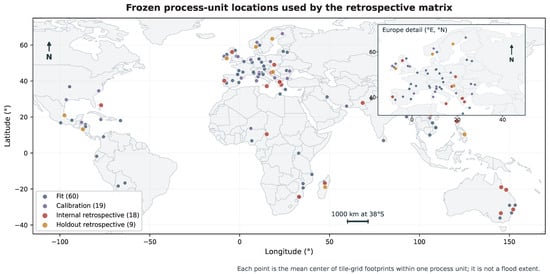
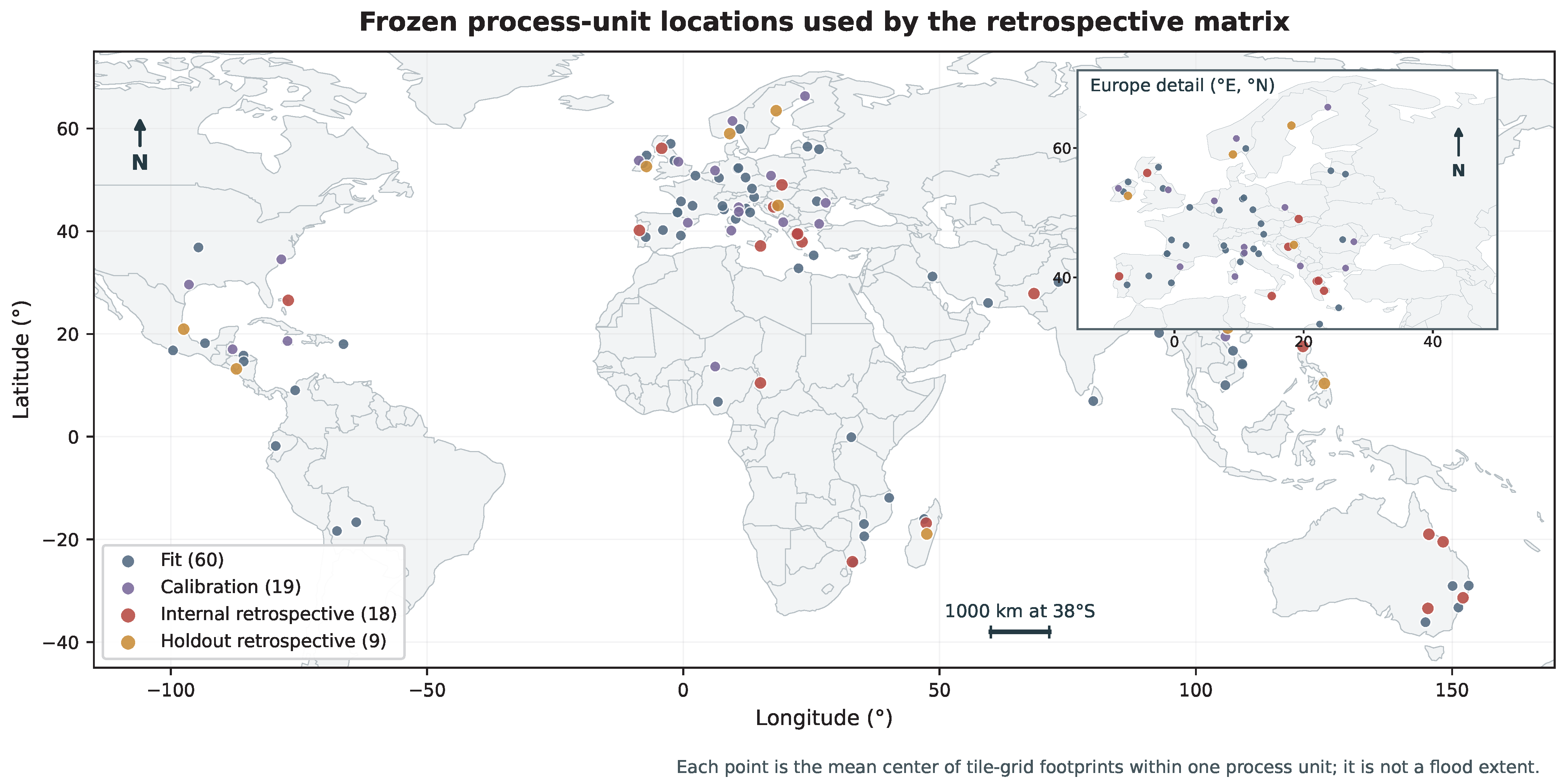
ImpactMesh’s data card does not identify each native mask’s CEMS product, version and reference-image time. Three fixed training-source vector checks gave native-flood overlap of 0.914, 0.873 and 0.961 for EMSR156, EMSR640 and EMSR424, respectively, but cannot identify the publisher’s historical product or verify the corpus. The later source audit found no confirmed tile-level chain for the main 18/9 evaluation roles. Their label reference times remain UNVERIFIED. We, therefore, evaluate prediction of dataset-native classes. Figure 2 and Appendix A document geographic support.
Figure 2.
Geographic support of the frozen three-seed roles. Points are mean tile-footprint centers within grouped processes, not flood extents or independent pixel samples. The European inset resolves the densest cluster. Coordinates are WGS84; the 1000-km scale applies along 38°S. Natural Earth supplies the public-domain backdrop. The distribution is uneven and does not establish regional representativeness.
2.2. Compared Systems and Training History
Table 1 answers two design questions: which information each system receives, and which architectural or training change separates it from its reference. B2 versus B4 is the central radar-only/fusion comparison. B5 and P test proposed defenses against missing optical input; B1 supplies a simple SAR-change reference. The parameter column makes the capacity difference explicit before any performance comparison. Neural models use a small U-Net [20] with feature widths 16, 32 and 64, two max-pooling stages, and two padded 3 × 3 convolution–GroupNorm–ReLU operations per block. Four-group normalization is used throughout. Bilinear upsampling, skip concatenation and decoder widths 32 and 16 precede a three-logit 1 × 1 output. Ordinary fusion separately encodes two-channel S1 and 12-channel S2, concatenating and reducing features with 1 × 1 convolutions at each scale. Optical invalidity is filled with normalized zero; wholly absent S2 additionally has its encoder features suppressed. The gate receives validity, presence and signed age normalized by 30 days, with zero age when S2 is absent.
Table 1.
Model key. All neural systems predict the same three classes. Parameter counts are for the small width-16 networks; the SMAGNet-style adaptation is a separate disclosed comparator.
All controlled neural comparisons share the raw paired fit pool; B2 uses its S1 counterparts. Normalization and class weights use fit-role samples only. B1 fits event-water and pre-to-event VH-change thresholds on training processes. It provides a simple multi-temporal SAR reference, whereas B2 uses one event image; the study does not compare against a learned multi-temporal SAR family. B4 has 84,688 more parameters than B2; their contrast evaluates complete systems with different parameter counts.
The main analysis uses the later three-seed upgrade, frozen after earlier v1–v6 results had been viewed. Seeds 20261013–20261015 share 60 fit processes, 24 epochs, weighted cross-entropy plus 0.3 flood soft Dice, and eight deterministically ordered tile draws per process per epoch. Batch size is four, giving 2880 updates. Adam [21] uses learning rate 0.001 for epochs 1–6 and 0.0003 for 7–24. Final epoch-24 weights are evaluated without test-driven checkpoint selection. B5/P whole-S2 dropout probability is 0.25; B4 has none. Training used PyTorch [22] (2.14.0+xpu on XPU and 2.5.1+cu124 on CUDA). The recorded execution includes XPU-to-CUDA migration and technical recovery. Fixed seeds do not imply bitwise determinism, and device changes are runtime provenance, not independent replications.
Historical stages are retained rather than pooled into these seeds. Formal v1 used one seed, eight epochs, cross-entropy, final weights and 0.5 dropout for B5/P. Its final calibration/internal populations each had 19 processes and its paired holdout eight. v2–v5 were post-test development; v6 reused a development fold with changed loss, checkpoint and calibration policies. The upgrade added three-seed B5 whole/local masking, P and an author-code SMAGNet-style adaptation with ResNet-50 and a two-head training loss. The adaptation reports its fused head, not an unmodified published checkpoint or a directly comparable published score. Appendix A.1 summarizes the stages and populations; complete rules and adverse historical outputs remain in the accompanying evidence package.
2.3. Optical Interventions, Calibration and Paired Scoring
Each paired tile is divided into 64 contiguous 32 × 32 blocks. A deterministic nested order keeps 64, 48, 32, 16 or zero blocks, intersected with the original joint validity mask V:
Original cloud, shadow and nodata never become valid. Thus 100% means no added masking, whereas 0% supplies absent S2. Nominal block retention differs from whole-grid valid coverage and original-valid-pixel retention:
At 100%, process-equal actual coverage is 90.06% internally and 86.53% on holdout. At 25%, it is 22.53% and 21.53%, while valid-pixel retention is 25.02% and 24.89%. The state labels describe the designed block intervention. Appendix A retains all five coverage states and distinct natural strata.
Within a process, lexicographic tile ownership counts each same-CRS pixel center once. All models share owned, non-Ignore scoring pixels . Counts and probability-loss sums are pooled over those pixels before calculating process metrics. Every process then receives equal weight. With class probabilities q and three-class argmax , the primary endpoints are
Flood intersection over union (IoU), , measures reference/prediction overlap; flood Brier, , measures flood-probability squared error. Larger IoU and smaller Brier are better. A zero IoU denominator is undefined and omitted from that endpoint’s common-process mean. An absent true class has undefined conditional scores, but contributes zero to an all-pixel additive decomposition. Support counts accompany the summaries.
Each neural model/seed receives one positive global temperature, fitted by process-equal multiclass negative log-likelihood (NLL) on the separate 19-process calibration role at original optical support. It stays fixed across optical states and external checks:
Positive scaling preserves the three-class argmax, so it cannot improve three-class IoU. Multiclass Brier sums all three coordinate errors; flood Brier uses only the flood coordinate. Calibration is examined separately using reliability summaries. We also retain multiclass NLL, 15-bin expected calibration error, class IoU, precision, recall and flood average precision.
The paired gains are and , both positive for B4 benefit. For each endpoint, three matched seeds are averaged within process before processes are averaged. IoU pairing requires definition for both systems and all seeds. Descriptive 95% intervals use 10,000 paired-process bootstrap samples, seed 20261029, keeping each process’s seeds together. Pixels, tiles, masks and seeds are not independent event replicates.
At full and zero S2, reference-class contributions exactly partition the flood-Brier gain. For class with prevalence and conditional loss ,
We average these products, not the product of separate mean prevalences and losses. On permanent-water pixels, flood target is zero, so conditional loss equals ; direct and permanent-to-flood argmax rates are calculated separately from fixed-model outputs. This arithmetic error partition is not Murphy’s reliability/resolution decomposition [23]. Reliability diagrams use the native flood-label fraction within fixed probability bins, not independent hydrological measurements; Appendix A.3 defines binning, seed pooling, process weights, empty-bin handling and support.
2.4. Controlled and Reference-Definition Checks
Three post-review checks use separately locked protocols on the same viewed roles. An architecture-matched control retains B4’s 203,491 parameters but receives normalized-zero S2, true presence/validity and zero age throughout fitting, calibration and evaluation. It shares the fit data, seeds, loss, optimizer, 24 epochs and final-checkpoint policy. It can learn optical-branch biases and boundary priors but no scene-specific optical information. Zero first-layer inputs reduce its effective function class; equal parameter counts do not remove this limitation. Control training uses XPU versus historical B4 CUDA. A same-evaluation-backend check and runtime records are retained; training-device and optimization differences remain.
A fixed-checkpoint input-policy check chooses the nearest eligible S2 from the unchanged 30-day/50%-valid pool, reusing original temperatures. It changes age and valid area jointly. Three hash-selected fit-only cloud/shadow donor masks, one per seed, provide another check. Donors cover 25–50% of the source grid, exclude nodata, and are intersected with recipient validity without translation or rotation. Actual coverage is reported rather than assigning a nominal retention target. Seed and donor identities are coupled; uncertainty conditions on these three fits and shapes. A nested smooth-field irregular mask additionally retains approximately half the originally valid pixels at its 50% label. Neither irregular nor transferred masking reproduces the joint cloud, rainfall and flood-generation mechanism.
The upgrade’s training/calibration stress test defines A/B as B5 whole-modality dropout and C/D as the same policy plus local contiguous masking. A/C use original-state calibration; B/D each use one global temperature fitted across five equally weighted states. A/B share weights, as do C/D. The prespecified flood-Brier interaction is , averaged equally over states within process; negative would support the proposed synergy. The full-input flood-IoU guardrail has a project-defined lower tolerance of . These remain descriptive checks on previously inspected processes.
A separate source-definition sensitivity assesses label-time uncertainty. Its 24 IDs were fixed from training-source temporal-audit cases, including 11 native-zero- flood cases; 19 belong to formal training and five were excluded. Available same-activation CEMS versions, stages and source tables define candidates, with current flood, previous flood and flood trace kept distinct. Rasterization uses unchanged native pixel centers. A strict geometry rule first retained failures as undefined. After that source-only negative result and before new model scoring, one documented uniform MakeValid amendment retained polygon components without an area cutoff. Fixed B2/B4 models then supplied 123 prediction calls without refitting. Within each candidate’s common native-non-Ignore/AOI domain, polygon complement means unmapped by that definition, not verified non-water. The squared probability discrepancy Q and set IoU, therefore, measure cartographic agreement, not physical flood accuracy or calibration. Appendix A.5 retains strict failures and all candidates.
2.5. External Endpoints and Their Admissible Interpretation
The earlier formal Sen1Floods11 test used 90 manually checked S1 tiles and no S2. Summed probability is evaluated against water/non-water labels. Spain and Nigeria have credible same-event risk with training activations; excluding their entire events leaves eight events in the main summary, with all-event sensitivity retained. This previously evaluated binary zero-S2 endpoint assesses water/non-water transfer.
A later exposure audit identified the separate 15-scene Bolivia split (15 February 2018) as previously unscored in recovered study records. All 15 whole scenes were locked before new scoring, without class- or performance-based selection. Original three-seed B2/B4 weights, fit-only statistics and global temperatures yield 90 forwards, with S2 absent. Unique finite-S1, non-Ignore pixels are pooled within the single event. Water is predicted at . Binary Brier uses the two-coordinate convention ; binary NLL clips true-class probabilities at under this newly locked scoring rule. Temperature preserves three-class argmax but can change the summed-water threshold decision. Reported seed ranges are not event confidence intervals. The shipped optical data lack the required Level-2A/SCL semantics, and same-day metadata do not establish pre-S1 order, so this check uses no S2. Its sigma0 dB input differs from the training RTC gamma0; exact SAFE identity and acquisition seconds remain UNVERIFIED.
The released Kuro Siwo expert reference explicitly supplies non-water, permanent water and flood [24,25]. The first eight metadata-complete labeled groups in pinned shard order were fixed before target pixels or new outputs, including two indexed pilot groups. They form one incomplete EMSR118/AOI01 event subset. Reference date is 2 February 2015 and post-S1 source day 3 February; exact UTC and SAFE identity remain UNVERIFIED. Published 0/1/2 labels are preserved, with source-invalid pixels ignored. Native 224 × 224, EPSG:3857 10-m projected grids remain unresampled. Finite positive VV/VH sigma0 is converted to dB and normalized using original fit statistics. Lee-filtered sigma0 versus training RTC gamma0 remains a transfer-domain difference. The six fixed B2/B4 fits receive zero S2, producing 48 forwards. Unique common valid pixels are pooled within the event subset; stable float64 log-softmax provides unclipped multiclass NLL. All seeds and adverse outcomes are retained without event-population intervals. These expert references are SAR-informed. Three selected tiles revisit geography used in earlier EMSR279 development, despite no actual membership of that event in the three-seed roles. Appendix A.6 explains the complete seed scores in Supplementary Tables S8–S10; exposure, source, processing and support are specified here and in the accompanying evidence records for both checks.
3. Results
3.1. When Adding Optical Imagery Improves the Flood Product
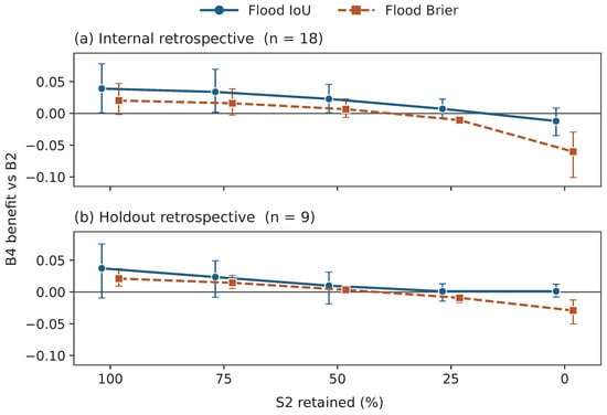
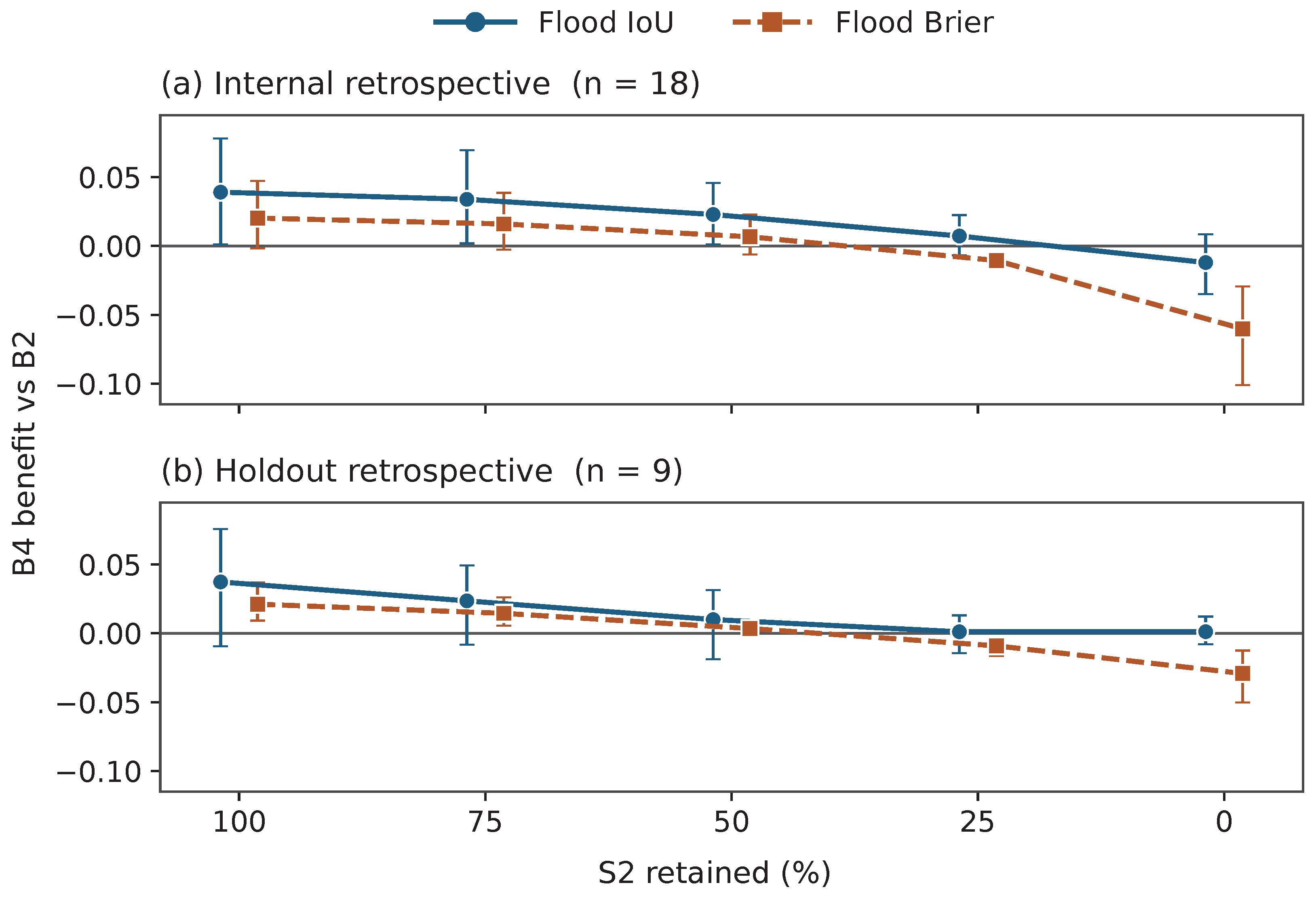
The answer to whether mapping improves is conditional: with the original optical input, fusion has better mean reference flood overlap and lower mean probability error than radar alone, but this advantage is not uniform across episodes or optical conditions. Here B2 denotes the radar-only reference and B4 the ordinary radar–optical system; the gains below always compare these two systems on matched support. With no added optical masking, B4’s mean flood-IoU gains over B2 are +0.0391 on 18 internal and +0.0373 on nine paired holdout processes; flood-Brier gains are +0.0203 and +0.0211 (Figure 3; Supplementary Table S1). The internal full-input Brier interval [−0.0019,+0.0472] spans zero, so the favorable mean does not indicate uniform improvement. At 25% nominal block retention, mean IoU gains remain slightly positive, +0.0072/+0.0011, with intervals spanning zero, while Brier gains become negative, −0.0106/ −0.0091. At zero S2, they are −0.0602/ −0.0292. These predetermined states mean locate a descriptive sign change between the 50% and 25% states.
Figure 3.
Joint flood-IoU and flood-Brier gains for ordinary fusion relative to radar alone. Positive favors fusion. Symbols are three-seed, equal-process means; whiskers are descriptive 95% paired-process bootstrap intervals. Nominal percentages denote retained spatial blocks, not actual valid coverage (Equation (2)).
The joint curve should be read by comparing the two outcomes at the same retention state. Better overlap means the thresholded flood map agrees more closely with the native reference; better Brier means the assigned flood probabilities have smaller squared errors over all scored pixels. These need not move together. At the quarter-block state, fusion still retains a small mean overlap advantage while its probabilities are worse. The complete five-state values and process outcome counts are supplied with measured optical coverage in Supplementary Table S1, so the figure’s state labels can be checked against actual input support.
At full retention, fusion improves both outcomes in 12/18 internal and 7/9 holdout processes; at zero, only 2/18 and 1/9 improve both, while 11/18 and 6/9 worsen both. Thus, the favorable full-input means conceal process-to-process variation, and removing S2 changes more than the average magnitude: fewer processes benefit on both endpoints. Every process remains in the appropriate supported summary. Naturally low-visible holdout cases also show different metric directions: B4/B2 mean flood IoU is 0.18289/0.15437, but flood Brier is 0.07763/0.07445. The one no-qualified-S2 process has only 95 native flood pixels among 708,120 scored pixels; both IoUs are near zero, and B4/B2 Brier is 0.09948/0.05917. Different case composition and small process support prevent treating these as replications of synthetic optical removal.
3.2. Class Contributions and Direct Permanent-Water Probabilities
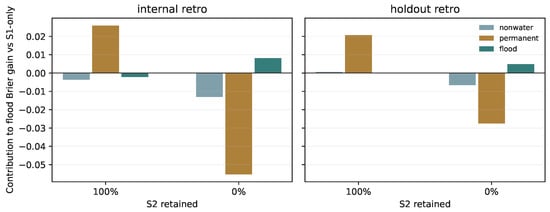
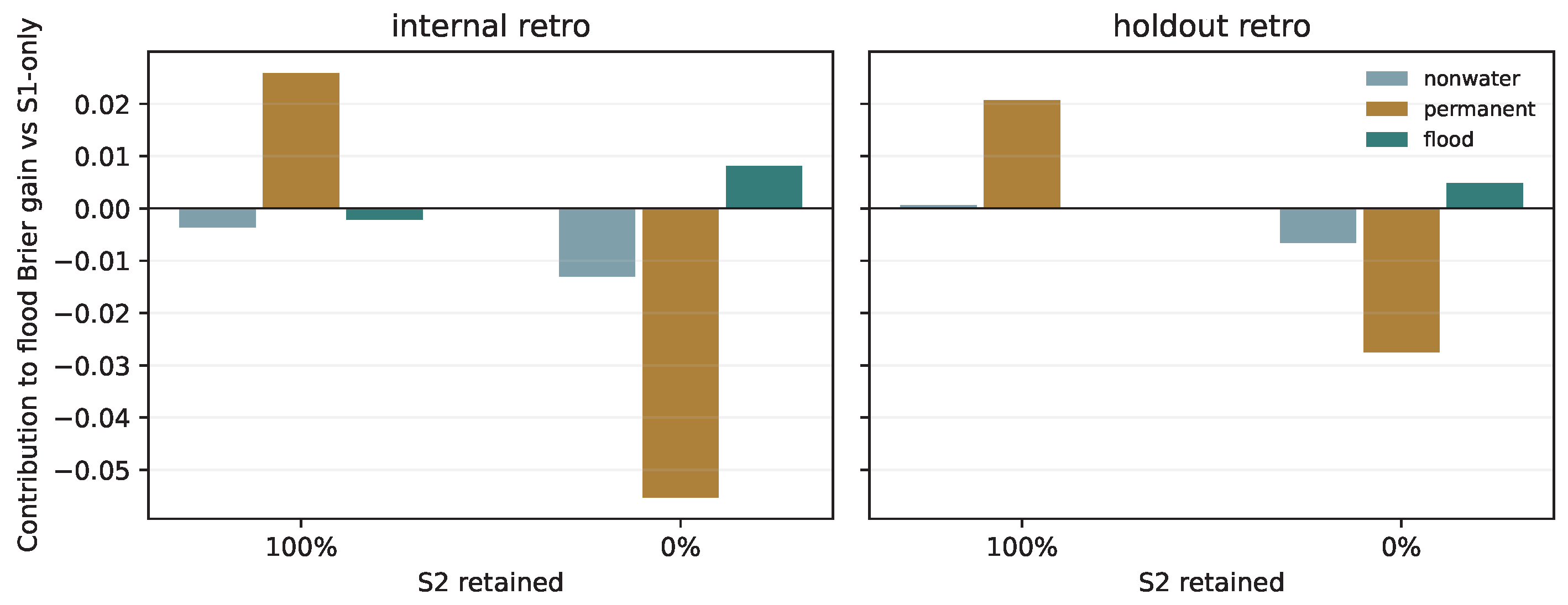
Native permanent-water pixels supply most of the favorable full-input flood-Brier contrast (Figure 4). Their contributions are +0.0259 internally and +0.0207 on holdout, compared with all-pixel gains +0.0203/+0.0211. True flood contributes −0.0021/ −0.0001, with intervals spanning zero. The aggregate probability benefit is concentrated on permanent water. Figure 4 locates the source of the aggregate score change. Each bar is the class’s contribution to the all-pixel denominator; the three bars sum to the total gain. A permanent-water contribution can exceed the total when errors on other classes offset it. The overall gain and true-flood conditional errors, therefore, answer distinct questions. Appendix A.2 retains the associated class prevalence and conditional errors.
Figure 4.
Native-reference-class contributions to the paired flood-Brier gain. Bars average three fixed seeds within a process, then average equally across processes. Positive values favor fusion; the three classes reconstruct the total. Full and zero S2 use identical owned scoring pixels.
Permanent water represents 13.7% of process-equal internal composition, yet its conditional flood Brier falls from 0.2836 for B2 to 0.1256 for B4. On holdout, it represents 8.3%, and the conditional score falls from 0.3297 to 0.1237. Conversely, true-flood conditional scores change from 0.3565 to 0.3594 internally and 0.1954 to 0.1995 on holdout, supported by 17/eight flood-bearing processes. Prevalence and within-class errors jointly determine the contribution; average prevalence alone is insufficient.
At zero S2, permanent-water contributions reverse to −0.0553/ −0.0275, while non-water contributes −0.0131/ −0.0065. True-flood contributions of +0.0081/+0.0048 partly offset these losses. Permanent conditional scores rise to 0.6004/0.6122, while true-flood conditional scores improve to 0.2543/0.0956. The 162 process/seed/endpoint class-sum checks reproduce the earlier total differences within 2.3 × 10⁻⁸.
Table 2 then asks a different question: how much flood probability is assigned to permanent water, and how often does that assignment become a hard flood label? Read its columns separately. measures the average assigned probability; measures conditional flood Brier because the reference flood target is zero here; the confusion column counts the fraction receiving the flood argmax. Together they distinguish soft probability leakage from a discrete class error. At full optical support, calibrated mean flood probability on permanent water falls from 0.451119 to 0.238210 internally and 0.520380 to 0.261883 on holdout. At zero S2, B4 means rise to 0.692926/0.713121. The corresponding permanent-to-flood argmax rates fall from 57.4%/71.4% for B2 to 20.1%/20.4% for full-input B4, then rise to 78.0%/79.5% at zero S2.
Table 2.
Direct flood-probability moments on owned, non-Ignore native permanent-water pixels. Each entry averages three seeds within a process, then supports processes equally (n). Raw uses temperature one; cal uses each model/seed’s original global temperature. The calibrated second moment is conditional binary flood Brier. Confusion is the three-class permanent-to-flood rate, common to raw/calibrated predictions. B2 consumes no S2 and is evaluated once, applying to both optical states. No new intervals or independent reference are introduced.
These moments use 12,084,942 internal and 1,524,065 holdout permanent-water pixels, with support reproduced exactly. Independent aggregation agrees within 2.23 × 10⁻¹⁶. Five jobs differ from historical hard counts by one pixel, with maximum rate difference 8.17 × 10⁻⁶ below the locked tolerance; its cause remains unresolved. Original scaling slightly lowers full-input B4’s first moment but increases its second moment from 0.123943 to 0.125641 internally and 0.122655 to 0.123679 on holdout. The first and second moments, therefore, provide complementary probability diagnostics.
3.3. Spatial Workflow and Opposing Errors
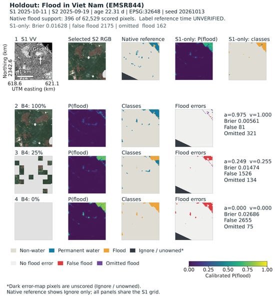
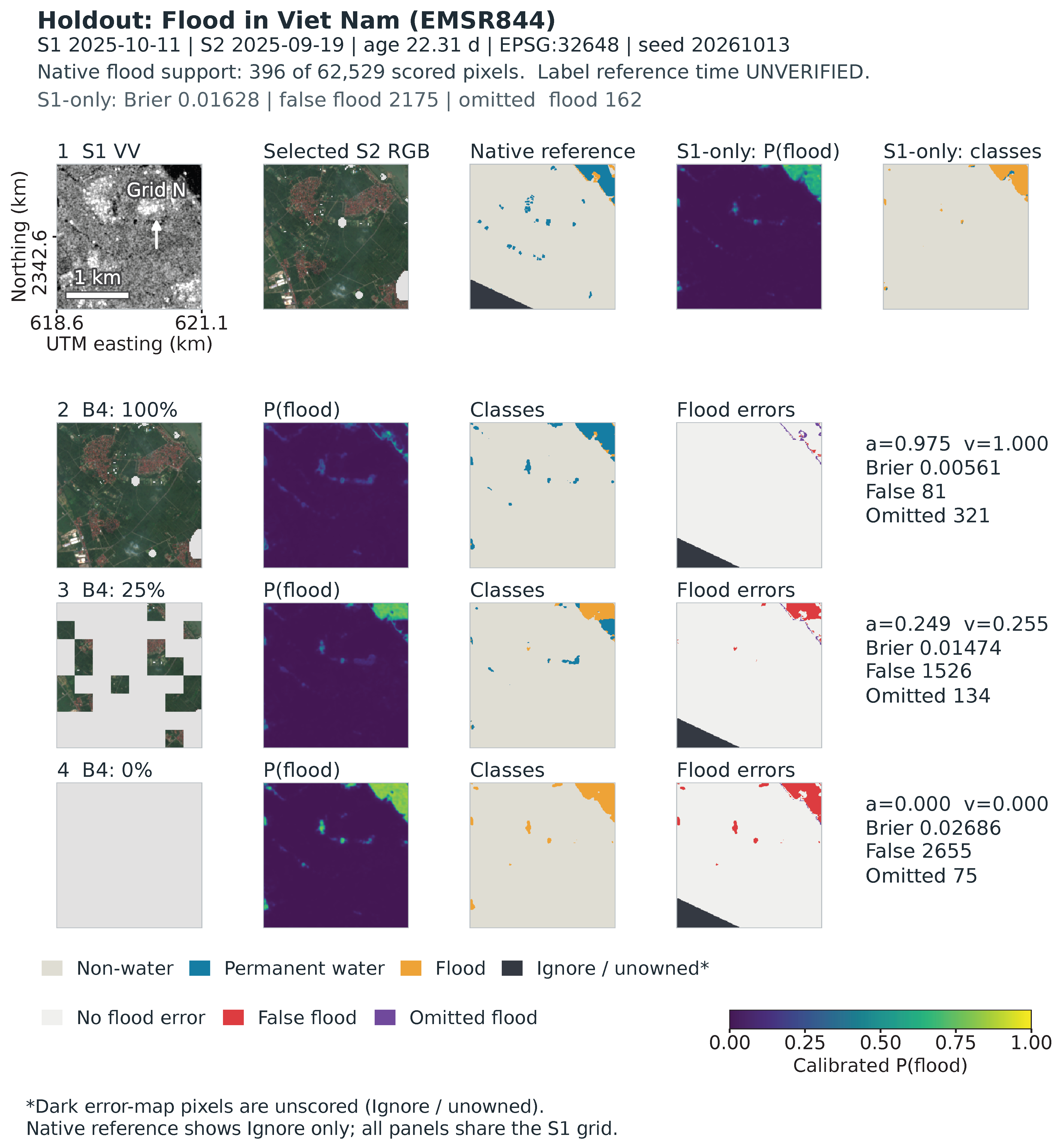
Figure 5 follows the fixed mapping workflow through observations, native references, predictions and errors.
Figure 5.
Observed inputs, native reference, predictions, probabilities and flood errors for metadata-selected tile EMSR844_1_48QXJ_x618565_y2343875, EPSG:32648. Fusion uses nominal 100%, 25% and 0% block retention; the shared probability scale is 0–1. Original temperatures and seed 20261013 are fixed. The 1-km scale, grid north and coordinates apply across panels; a and v follow Equation (2). Dark error pixels are Ignore or unowned. Native label time remains UNVERIFIED.
The metadata-hash-selected holdout example in Figure 5 comes from the October 2025 Viet Nam activation EMSR844. S1 was acquired 11 October; selected S2 is 22.31 days older. Among 62,529 scored pixels, 396 are native flood and 2817 permanent water. Full-input fusion predicts 61 permanent pixels as flood, versus 2206 at zero S2. At the same time, omitted native-flood pixels decrease from 321 to 75. Loss of optical support can, therefore, increase false flooding while reducing omissions within the same scene.
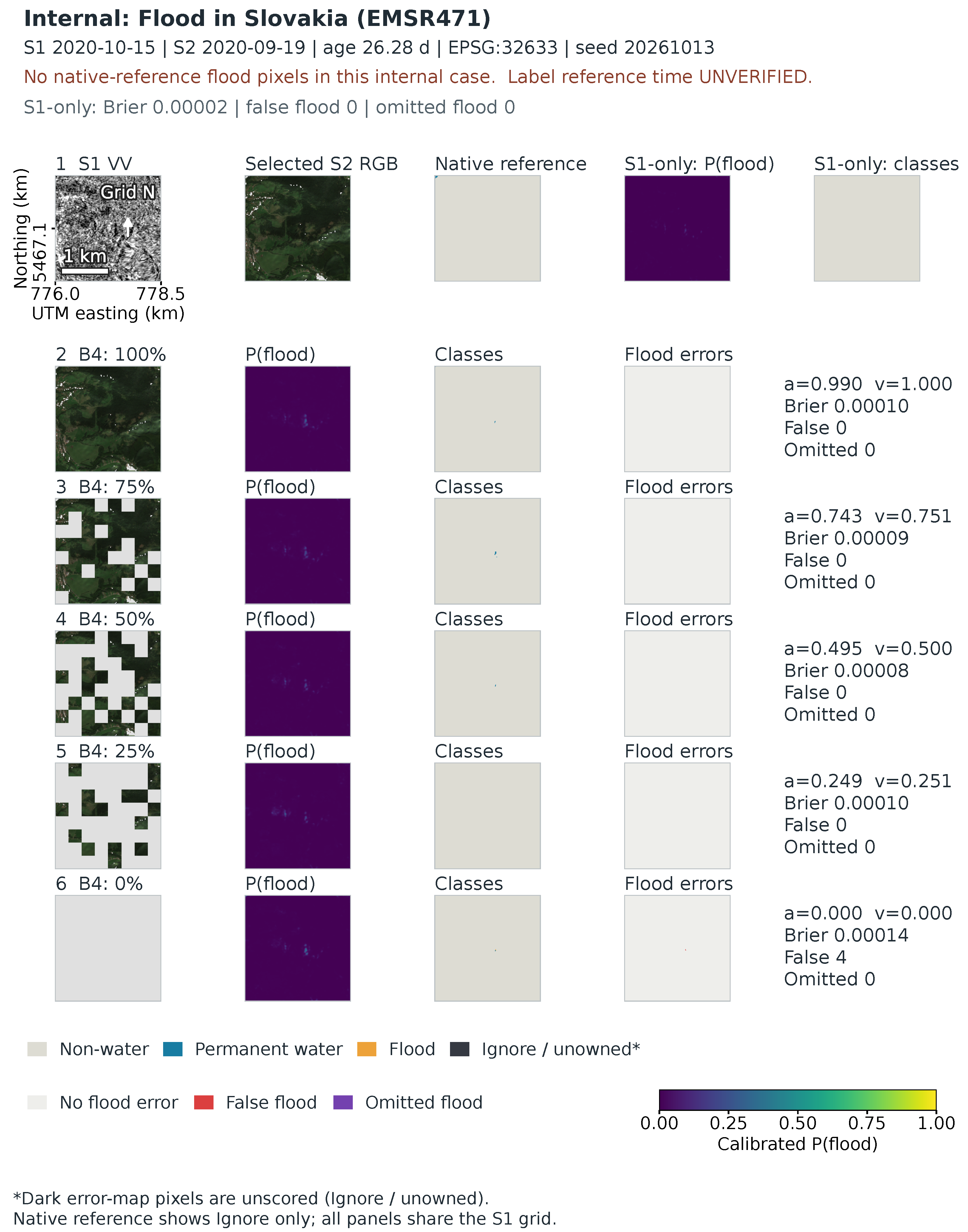
The independently metadata-selected internal example, EMSR471 from the October 2020 Slovakia activation, has no native flood. It is retained rather than replaced after label inspection. Appendix A shows both complete five-state sequences, including that no-flood case.
3.4. Capacity, Acquisition and Masking Sensitivities
The controls in Table 3 test three possible explanations for the main result: extra network parameters, the rule used to choose an optical acquisition, and the geometry of added missingness. The first two rows compare fusion against an architecture-matched constant-input system. The other rows change B4’s input policy while retaining its trained weights, so their contrast signs differ: lower Brier in those rows favors the alternative policy. These checks refine the interpretation of the main curves.
Table 3.
Controlled sensitivities, with descriptive 95% paired-process intervals. Capacity rows are positive-favoring-B4 gains against the constant-input control. Policy/cloud rows are alternative minus original B4: positive IoU and negative Brier favor the alternative. All use the same 18 internal/nine paired holdout processes and original temperatures.
All three constant-input control fits completed. Relative to this 203,491-parameter control, full-input B4 retains positive mean IoU and flood-Brier gains (Table 3). The holdout IoU interval spans zero. These gains coexist with lower flood recall: B4 minus control is −0.0635 internally and −0.0803 on holdout, with intervals below zero on 17/eight flood-bearing processes. Precision increases by +0.0808/+0.0666 and permanent-water IoU by +0.3351/+0.5140. The gains reflect higher precision alongside lower recall. Against the control, B4 Brier gains become −0.0137/ −0.0115 at 25% blocks and −0.0633/ −0.0316 at zero, with both zero-state intervals below zero. Effective capacity and training runtime remain confounded.
Nearest-acquisition selection changes 301 internal tiles in five processes but only two holdout tiles in one process. Mean effects are small and mixed; the holdout intervals touch zero because some bootstrap samples omit the sole changed process, reflecting the concentration of the input change in one process. Younger inputs also have less valid area. Three transferred training-cloud shapes worsen Brier in both roles, while IoU intervals span zero (Table 3); precision falls and recall rises. Age, area and shape vary jointly in these checks. At the 50% labels, irregular minus regular B4 Brier is +0.0008 internally and −0.0006 on holdout, with IoU changes +0.0001/+0.0029. The different retained-area denominators limit interpreting these small differences as shape robustness.
3.5. Negative Training and Calibration Results
The upgrade completed 18 neural fits, 24 global-temperature fits, 48 neural role evaluations and two B1 evaluations. Its prespecified B5 interaction is +0.000245, interval [+0.000108,+0.000410], opposite the hypothesized negative direction. One seed is slightly negative and two are positive with respective interaction estimates −0.00005, +0.00052, and +0.00026 for seeds 20261013, 20261014 and 20261015. The positive mean and its positive interval mean that the specified training–calibration combination misses the intended probability target.
At full input, C and A have nearly equal internal flood IoU, 0.28790/0.28799. The interval is [−0.01403,0.01463], and its one-sided lower bound −0.01166 exceeds the project tolerance −0.02; indicating descriptive compatibility with the project guardrail. At zero S2, C improves IoU over A, 0.22835 versus 0.20820, but worsens flood Brier, 0.06617 versus 0.06387. Radar-only and the SMAGNet-style comparator have higher zero-state IoU, 0.25505/0.25337. The holdout likewise gives C/A zero-state IoU 0.23916/0.21637 but Brier 0.05046/0.04668. Local masking does not achieve the probability target.
The earlier formal benchmark also gives no gated-model advantage: internal full-input IoU is B4 0.297, B5 0.287, P 0.252, B1 0.206 and B2 0.164; paired P-minus-B4 is −0.045 [−0.064,−0.026]. P’s near-flat retention curve starts lower. The later B4 flood-Brier raw/scaled values are 0.04750/0.04785 at full input and 0.12580/0.12834 at zero. Multiclass-NLL temperature fitting, therefore, guarantees neither a flood-Brier gain nor transfer across availability states. In formal v1, B4’s NLL scaling benefit weakens from −0.0202 at full input to +0.0044 at zero, a paired interaction +0.0246 [0.0125,0.0377], although the zero-state absolute-change interval spans zero. Complete historical outputs remain in the accompanying evidence package; stage and reliability summaries are in Appendix A.1 and Appendix A.3.
3.6. Source-Definition Dependence and External Endpoints
Under the strict source recipe, only eight fixed cases had evaluable common domains and each had one unique candidate mask; seven were empty in both source membership and native flood. The strict recipe, therefore, provides no within-case source variation. The uniform geometry amendment makes 15 common domains evaluable, comprising 25 current-flood unions, 31 source slices and six previous-flood definitions, not independent events. Five cases have current-union variation; eight have only empty unions. All 123 fixed prediction calls completed and saved-probability scoring was independently reproduced.
Reference choice reverses some local orderings. With positive favoring B4, EMSR637’s original-temperature range is [−0.075690,0.005649] at zero S2 and [−0.073146,0.010814] at original S2. EMSR640 also crosses zero in original-S2 ; its zero-S2 IoU gain ranges from −0.006922 to +0.029152. Its native-definition squared-discrepancy gain is positive at zero S2, whereas every current-union value is negative. At least one current union gives adverse zero-S2 in 12/15 cases with original temperatures. On the same 11 S2-eligible cases, original S2 reduces B4 discrepancy for all 18 current-union definitions. These results characterize sensitivity to cartographic definitions and dates.
Table 4 is organized by the question each reference can answer. Bolivia tests transfer of water/non-water mapping; Kuro tests the separation of the three native classes. They are distinct single-event endpoints, with different probability-loss definitions, and their numerical loss magnitudes should not be compared across datasets. Within each block, the B2/B4 contrast shows whether a favorable average persists outside the main retrospective roles. Complete per-seed values are separated into Supplementary Tables S8–S10 to keep mixed and adverse fits visible without interrupting this comparison.
Table 4.
Additional external endpoints with original temperatures. Values are means of three fixed seeds within one event/subset, with no event confidence intervals. Bolivia water Brier is the two-coordinate binary sum; Kuro sums three coordinates and uses only the flood coordinate, so losses across targets are not interchangeable.
The separately locked Bolivia run completes all 15 scenes and 90 forwards. Its 2,824,434 common valid unique pixels include 451,901 water and 2,372,533 non-water. With original temperatures, mean water IoU is 0.6759 for B2 and 0.6577 for B4; binary Brier is 0.1135 for B2 and 0.1253 for B4 (Table 4). Paired B4 benefits are −0.0182 for IoU (seed range [−0.0488,+0.0103]) and −0.0118 for Brier ([−0.0362,+0.0099]). Seed directions are mixed. Raw probabilities also favor B2 on average; original calibration improves B2 but slightly worsens B4’s probability losses. This provides an additional binary zero-S2 transfer endpoint in a different SAR processing domain.
All eight Kuro tiles and 48 forwards are also complete. Common support is 361,852 unique pixels: 327,535 non-water, 2484 permanent water and 31,833 flood. Both water classes occur only in the sixth selected tile; the other seven remain in the denominator. B4 has higher flood IoU in all three fits, but permanent-water IoU is zero in every fit. Its higher mean permanent-to-flood rate and flood probability expose adverse class transfer despite favorable full-multiclass Brier. Flood-coordinate Brier instead favors B2. Full multiclass Brier combines all class coordinates, so flood-coordinate loss and permanent/flood separation provide complementary diagnostics. Hard-confusion and flood-Brier differences have mixed seed directions; for seeds 13/14/15, permanent-to-flood counts are 21/57/1941 for B2 and 2241/2126/1926 for B4, out of 2484 each. Temperature worsens both models’ mean multiclass and flood-coordinate losses here while leaving three-class hard labels unchanged. All raw, scaled and per-seed results remain in Supplementary Tables S8–S10, with interpretation in Appendix A.6.
A supplementary one-seed EMSR871 check uses only 883 CEMS mapped-positive pixels, retained from 37,983 initial positives by a complete-valid-crop rule. Zero-S2 B2/B4 omission is 0.91393/0.03624, with conditional positive squared loss 0.48575/0.07652. This severe support restriction, absence of reviewed negatives/permanent water and shared SAR dependence prevent full-domain IoU, calibration or three-class validation. Its source and failure records remain in Appendix A.5; interpretation is conditional on the retained mapped-positive support.
4. Discussion
4.1. What Optical Availability Changes in These Fitted Systems
The class accounting separates changes in flood-probability error by reference class. Full-input gains are mainly lower flood probabilities on native permanent water, while true-flood conditional errors do not consistently improve. At zero S2, permanent water supplies the largest loss and true flood partly offsets it. This is compatible with a trade-off between omissions and false flooding, illustrated spatially and reinforced by the constant-input control’s precision/recall contrast. The class decomposition describes error changes conditional on the native references. Three-class confusion, first moments, conditional second moments and prevalence-weighted contributions answer distinct questions; their agreement should be checked explicitly.
The constant-input control matches the declared architecture and training schedule, and the favorable full-S2 mean persists. Effective capacity and training devices differ between systems. Nearest selection changes coverage and age together, while cloud transfer changes area and shape together. The 50–25% sign change describes the tested optical-input states.
A user comparing radar-only and fused products should ask two questions: does the mapped flood area agree better with the reference, and do the supplied probabilities also have smaller errors? For probability layers used to rank locations for further inspection, probability error and hard-map overlap should be evaluated together. In these experiments, lower false-flood probabilities on permanent water account for much of the original-optical benefit, while true-flood conditional errors vary across episodes. The practical recommendation is to report optical support, both outcome measures, and permanent-water versus flood errors together. These image-mapping diagnostics provide a complementary perspective for evaluating forecast and inundation products.
4.2. Training and Calibration Responses
Whole-modality dropout, local masking and explicit availability gates are plausible defenses with metric-dependent effects in these experiments. The prespecified interaction within the retrospective upgrade has the opposite sign to the proposed probability benefit. A flatter retention curve can also begin at a lower complete-input score. Reporting only stability or zero-S2 IoU would obscure this cost. These outcomes characterize the specified architectures, budgets, seeds and calibration policies.
One global temperature provides a simple post-hoc baseline. It fits multiclass NLL at one input distribution and preserves three-class decisions. The multiclass-NLL objective, flood-coordinate Brier and permanent-water conditional loss assess different aspects of probability quality and transfer. Reliability-bin frequencies are empirical frequencies of the native reference labels; they inherit reference uncertainty and finite process support. Sparse high-probability bins warrant particular care. The retained support ledger prevents three seeds or many pixels from being mistaken for many independent floods.
4.3. Reference Provenance and Evaluation Scope
The main evaluation uses dataset-native labels whose tile-level CEMS product, version and reference-image UTC remain unverified. The source-definition sensitivity shows that public map choice can reverse some local model orderings, with cartographic definitions and dates varying together.
The 18 internal and nine holdout processes had been inspected during development, so the central optical-retention comparison is retrospective. Bolivia contributes one previously unscored binary event at zero S2, with mixed seed directions and a different SAR processing domain. Geographic support is uneven.
Kuro contributes a source-defined three-class event subset. Both water classes occur in one tile; some geography was used in prior development, the references are SAR-informed, and exact source times remain unknown. Zero permanent-water IoU and a high permanent-to-flood rate expose adverse transfer, alongside sigma0/gamma0 and preprocessing differences.
Together, these results show that optical support affects hard and probabilistic flood outcomes differently in the evaluated systems, with permanent-water errors dominating the aggregate probability contrast. Future evaluation should use unused multi-event populations with auditable reference times, compatible optical inputs and explicit flood/permanent-water references.
5. Conclusions
Adding Sentinel-2 optical imagery to Sentinel-1 radar improved average flood-area mapping and reduced flood-probability errors compared with radar alone when the original optical input was available. As optical information was removed, a slightly better mapped flood area could coexist with less accurate flood probabilities. Flood-area overlap and flood-probability quality should, therefore, be checked separately under the optical conditions in which the product will be used.
The contribution is an evaluation finding and class-specific explanation that help interpret radar–optical mapping results. Users should assess mapped extent and probabilities separately and state the optical support under which any benefit was observed. Controls expose recall trade-offs, training and calibration responses vary across metrics, and single-event external checks reveal transfer sensitivity. Broader evaluation can extend these findings using unused events, auditable reference times and compatible multisensor inputs.
Supplementary Materials
The following supporting information can be downloaded at: https://www.mdpi.com/article/10.3390/rs1010000/s1, Table S1: Five-state paired gains and actual optical support; Table S2: Geographic annotations of the retrospective evaluation support; Table S3: Descriptive process-age groups for the fixed B4–B2 comparison; Table S4: Native class prevalence and conditional flood Brier by fixed process-age group; Table S5: Class IoU at both optical endpoints by fixed process-age group; Table S6: Native permanent-water pixels predicted as flood by fixed process-age group; Table S7: Support behind the internal retrospective reliability diagrams; Table S8: Complete per-seed Bolivia event scores, including every planned model and probability version; Table S9: All 12 original-fit/probability-version records for the fixed eight-tile Kuro subset; Table S10: Complete seed-specific flood-coordinate scores and leakage for Table S9.
Author Contributions
Conceptualization, Z.G. and J.D.; methodology, Z.G. and C.Z.; software, Z.G.; validation, Z.G. and C.Z.; formal analysis, Z.G.; investigation, Z.G. and C.Z.; data curation, Z.G. and C.Z.; writing—original draft preparation, Z.G.; writing—review and editing, Z.G., C.Z. and J.D.; visualization, Z.G.; supervision, J.D.; project administration, J.D.; funding acquisition, J.D. All authors have read and agreed to the published version of the manuscript.
Funding
This research was funded by the Science and Technology Program of Hunan Province, grant number 2026AQ2031, and the Natural Resources Science and Technology Project of Hunan Province, grant number 20240131DZ. The sponsors provided financial support only and had no role in study design, data collection or organization, data analysis, interpretation of the results, manuscript preparation, or the decision to publish.
Institutional Review Board Statement
Not applicable.
Informed Consent Statement
Not applicable.
Data Availability Statement
The source datasets are available from the cited providers under their respective access and licensing terms. The original public code release is retained at https://github.com/ljm434782/rs-flood-reliability-code (accessed on 16 November 2026).
Acknowledgments
The authors take responsibility for the manuscript and the results.
Conflicts of Interest
The authors declare no conflicts of interest.
Appendix A. Supporting Design, Source and Transfer Checks
This appendix keeps the design history and interpretive checks needed to assess the main findings. Separate Supplementary Tables S1–S10 provide the complete coverage, geographic, age-group, reliability-support and single-event seed ledgers. They make denominators and exceptions inspectable alongside the main account.
Appendix A.1. Experimental History and Geographic Support
Table A1 distinguishes source pools from development frames and from tiles actually consumed during training. Its rows describe successive study stages. Formal v1 used eight epochs and seed 20260927. Its Irma/Boris safety exclusions were recorded after training started but before calibration/test scores; Nigeria overlap was identified after B1 output was written and before its numerical summary was inspected. Subsequent development and post-review checks retain their own protocols and exposure history. The SMAGNet-style adaptation is retained as an existing comparator.
Table A1.
Cross-stage sample ledger. Cells give native process units/tiles. Fit and development columns describe eligible paired pools, not the number of distinct training tiles consumed or tiles scored per epoch. Formal v1 original counts reconstruct the pre-amendment role assignment from metadata; the reconstructed holdout eligibility count is not represented as knowledge available before fitting. Complete results were not executed as one unamended test. The actual fixed development frames and temporal/exposure distinctions are given below.
The main three-seed row is the population used for the central curves. Earlier rows explain why similarly named roles elsewhere can have different counts; they must not be pooled. The 432 paired holdout tiles also include a two-tile EMSR841 unit that failed formal v1’s earlier five-tiles-per-activation reporting minimum. This accounts for a concrete population difference without revising either historical result.
Geographic support is uneven (Figure 2; Supplementary Table S2). Internal support includes four Australian units/321 tiles and three Greek units/529 tiles; the holdout parent includes 142 Irish and 121 Norwegian tiles, plus 110 tiles carrying the joint Honduras; Nicaragua annotation. These source country annotations document the uneven geographic composition of the process-equal evaluation.
Appendix A.2. Class, Optical-Age and Natural-Availability Support
Table A2 accompanies the main class-contribution figure. Read conditional loss b as the error within a reference class, and as its contribution to the full scoring denominator. The latter averages prevalence-weighted process errors; it is not obtained by multiplying the displayed mean prevalence by the displayed mean loss difference. Undefined class-absent conditional scores remain excluded from conditional means and contribute zero to the all-pixel sum.
Table A2.
Which reference classes account for the flood-Brier difference? Conditional errors use class-present process support ; prevalence and additive contributions use all 18 internal/nine holdout processes. Positive and favor B4. The three class contributions within each role/state sum to the total gain.
This table explains why permanent water dominates despite its smaller prevalence: its large conditional error reduction at full S2 outweighs the small adverse true-flood contribution. At zero S2, that permanent contribution reverses. True-flood conditional support is 17 internal and eight holdout processes, whereas IoU may remain defined in a process without true flood if false flood is predicted. The different support rules, therefore, have a practical effect on interpretation.
Supplementary Table S1 links all five nominal masking states to actual valid area. Internal coverage is 90.06, 67.56, 45.05, 22.53 and 0%; holdout coverage is 86.53, 64.94, 43.28, 21.53 and 0%. The corresponding valid-pixel retention is 100, 75.02, 50.02, 25.02 and 0% internally, and 100, 75.07, 50.03, 24.89 and 0% on holdout. These sequences distinguish a designed block intervention from observed cloud fraction.
The age tables answer whether the descriptive score pattern appears only among older optical inputs (Supplementary Tables S3–S6). Internal process counts in [0, 7], (7, 14] and (14, 30] days are 3, 2 and 13; holdout counts are 0, 1 and 8. Mean full-input flood-Brier gains are positive in every populated group (+0.0551/+0.0142/+0.0131 internally and +0.0080/+0.0228 on holdout), while all populated quarter-block groups are negative. This describes consistency across these sparse age groups. The recent internal group has only 1.7% mean native flood prevalence versus 10.0% in the oldest group; age, class composition and event identity vary together.
Table A3 answers a separate question: what happens on archived cases with naturally constrained optical availability? Its first two rows reuse identical pairs, while the last two use different cases. Their score differences, therefore, cannot be attributed solely to optical loss.
In the low-visible stratum, higher B4 overlap coexists with worse Brier, consistent with the need to inspect both endpoints. The no-qualified-S2 stratum contains only one process and 95 native flood pixels among 708,120 scored pixels; its near-zero flood IoUs are consequently a weak basis for general deployment claims. The table supplies a descriptive check of naturally constrained optical availability.
Table A3.
Fixed B2/B4 performance on paired synthetic and naturally constrained optical populations of the retrospective holdout. Paired 100%/0% use the same 432 tiles/nine processes; natural low-visible and no-qualified-S2 groups use 49/five and 11/one, respectively. All entries use the original one-global-temperature policy. These are different populations, not a natural-versus-synthetic causal estimate or an operational fallback rule.
Appendix A.3. Reliability Frequency and Support
The reliability diagram (Figure A1) asks whether predictions assigned similar flood probabilities have similar native-reference flood frequencies. It uses 15 fixed bins , with the last including one. Let pool three seeds’ prediction/reference pairs within process p and bin j on common owned non-Ignore pixels. For nonempty bins,
where contains processes supporting the bin. Empty bins remain undefined. These are empirical frequencies of native labels, not synchronized hydrological measurements. Process support can differ between bins and systems. The 10,000-draw bootstrap uses seed 20261029 and retains three fits together. This differs from maximum-confidence multiclass ECE.
Figure A1.
Flood-probability reliability with no Sentinel-2 observations retained. The vertical coordinate is the native-reference flood frequency calculated using the aggregation described above. Shaded bands match the colors of the corresponding curves and show pointwise 95% percentile bootstrap intervals obtained from 10,000 resamples of flood processes. The bands can overlap, producing blended colors. No interval is shown for the highest probability bin because some bootstrap resamples contain no process contributing predictions to that bin; the point estimates are retained. Varying process support and unresolved reference timing limit physical interpretation.
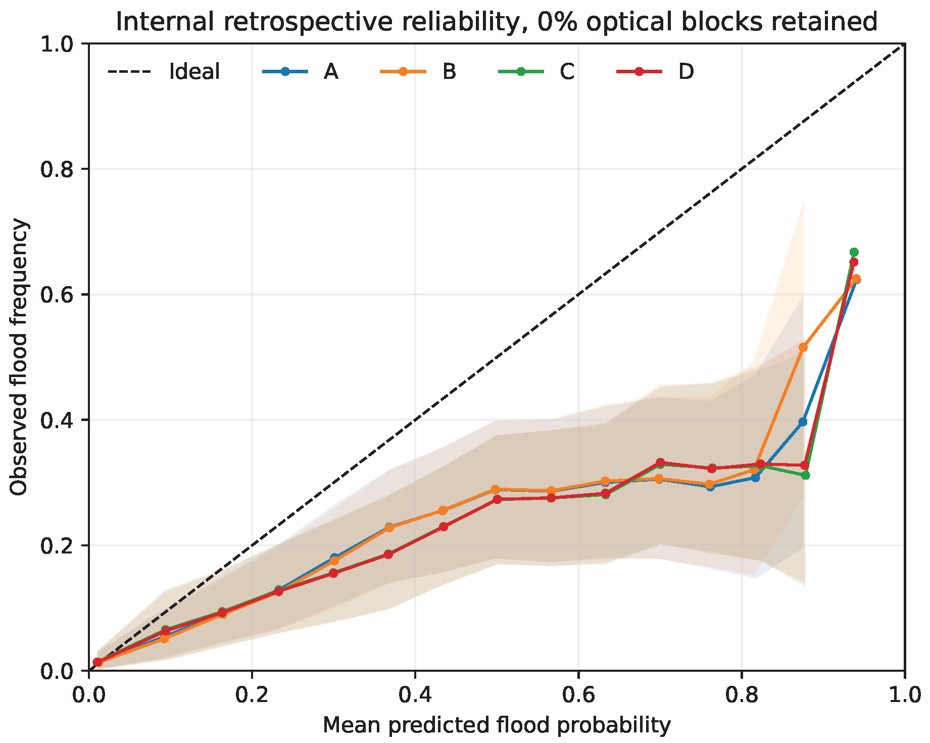
Supplementary Table S7 states how much evidence supports this diagram. Each arm/state has 118,478,007 unique scored pixels, represented by 355,434,021 pixel–prediction pairs across three seeds. At zero S2, some bins contain only three supported processes for arms A/B or five for C/D, despite all 15 bins being populated overall. A smooth-looking curve or a large pixel count must, therefore, not be read as uniformly strong process-level evidence. The retained CSV reconstructs all 240 audited bin rows.
Appendix A.4. Complete Spatial Examples
The complete sequences show how the opposing errors develop across all five optical states. The holdout sequence (Figure A2) extends the main spatial figure; the internal example (Figure A3) deliberately retains its zero native-flood support. Metadata-based selection followed prior role-level exposure; neither was replaced after inspecting labels or predictions.
Figure A2.
Complete five-state sequence for the main metadata-selected holdout case. Nominal block retention differs from whole-tile coverage and originally valid pixel retention. Original seed-20261013 weights, temperatures, ownership and Ignore support remain fixed. Native reference time is UNVERIFIED.
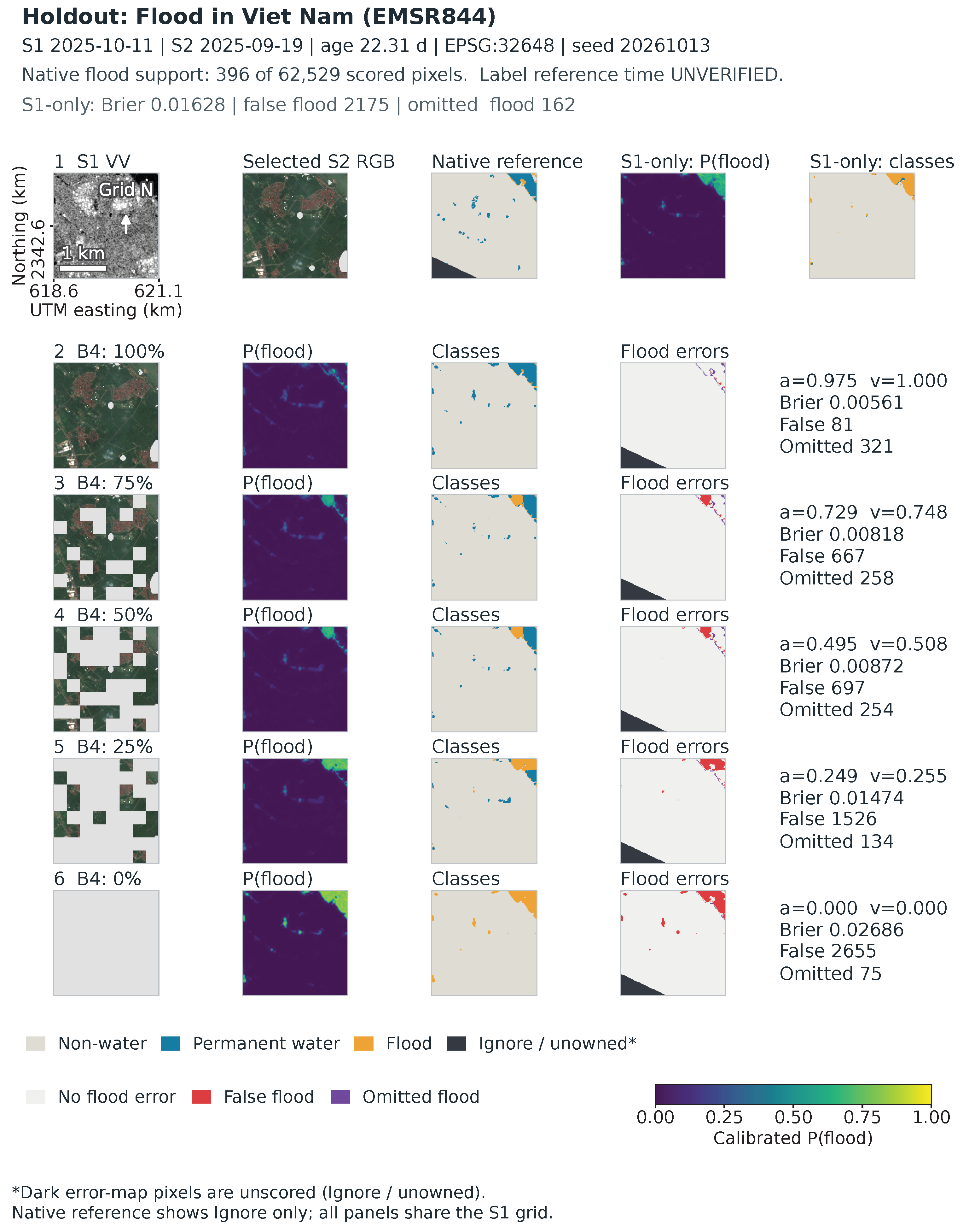
Figure A3.
Retained internal example EMSR471_4_33UYQ_x775955_y5468325, EPSG:32633, October 2020 Slovakia activation. S1 is from 15 October and S2 from 19 September (26.28 days earlier). Its 65,536 scored pixels contain 65,492 nonwater, 44 permanent water and zero flood labels. This illustrates false flooding without estimating flood sensitivity. Shared coordinates and scales are preserved; reference time is UNVERIFIED.
Appendix A.5. Source-Definition Sensitivity and Audit Limits
The fixed 24 training-source pilot IDs include 11 native-zero-flood cases: 19 are formal-training cases and five failed paired eligibility. Twenty-three newly obtained vector packages and retained archives provide 34 packages for 17 cases; 21 advertised URLs remain inaccessible. The strict representation yielded 77 successful and 68 failed slices, with overlapping case counts. Its eight evaluable cases contained only one distinct mask per case (seven empty, one with 13 mapped versus 17 native flood pixels). The strict recipe, therefore, yields identical within-case masks and scores.
After source-only inspection and before new model scores, one uniform MakeValid-linework counterfactual changed 313 of 13,252 feature WKBs; none of the 77 defined strict raster masks changed. It yielded 15 evaluable cases, 25 current-flood unions, 31 partial source slices and six previous-flood definitions. All 123 fixed-model calls completed. Independent reconstruction checked 1836 scores and 1224 contrasts (maximum difference ), with all 619 frozen identities unchanged.
For EMSR637, original-temperature discrepancy gains span to +0.005649 at zero S2 and to +0.010814 at original S2. EMSR640 also has source-dependent sign changes. All five source-varying cases, empty/undefined outcomes and same-domain comparisons remain in the accompanying case/version CSVs. Original versus zero-S2 comparisons use the same 11 eligible cases: squared discrepancy falls for all 18 applicable current-union definitions, while IoU changes are 10 positive, seven zero and one undefined. Outside a polygon within common support means UNMAPPED, not certified nonwater; outside common support is unscored. These conditional map-agreement results describe sensitivity to the retained source definitions.
The native MASK-to-product/version-to-source-UTC chain and export recipe remain UNVERIFIED. A fixed six-candidate new-event screen cleared zero complete reference/input gates; failures were retained. AI/source proxy products have zero scoring support under the earlier complete-crop rule. Their unsuccessful screening records are retained.
Appendix A.6. How to Read the Complete Single-Event Transfer Scores
Supplementary Tables S8–S10 preserve every planned seed and both raw and original-temperature probabilities. They answer whether a reported mean hides adverse fits or distinct calibration responses. They condition on one Bolivia event and one incomplete Kuro event subset, respectively; both use absent-S2 inputs and report within-event seed variation.
Bolivia sums permanent-water and flood probabilities and thresholds water at 0.5, so temperature can change the collapsed binary decision. Kuro uses three-class argmax, which positive scaling preserves; its identical raw/scaled IoUs are, therefore, expected, while probability losses can still change. The Kuro leakage ledger uses the same 2484 reference permanent-water pixels in every row. Its per-seed rates expose variation hidden by the mean, including B2’s adverse third seed. The six fits and 12 probability-version records quantify within-event fitting and scaling variation.
The portable source includes the used tables and figures, separate detailed tables, and updated responses. Dated protocols, selection/exclusion records, adverse outcomes and numerical audits are retained in the supporting materials. The original public release and the review-stage support snapshot retain separate version records.
References
- Notarangelo, N.; Wirion, C.; van Winsen, F. STURM-Flood: A curated dataset for deep learning-based flood extent mapping leveraging Sentinel-1 and Sentinel-2 imagery. Big Earth Data 2025, 9, 412–438. [Google Scholar] [CrossRef] [Scilit]
- IBM–ESA Geospatial. ImpactMesh-Flood, Version 1: Dataset Card. Version v1 Identified on the Official Dataset Card; Technical Report Described There as Forthcoming. Available online: https://huggingface.co/datasets/ibm-esa-geospatial/ImpactMesh-Flood (accessed on 22 October 2026).
- Nearing, G.; Cohen, D.; Dube, V.; Gauch, M.; Gilon, O.; Harrigan, S.; Hassidim, A.; Klotz, D.; Kratzert, F.; Metzger, A.; et al. Global prediction of extreme floods in ungauged watersheds. Nature 2024, 627, 559–563. [Google Scholar] [CrossRef] [Scilit] [PubMed]
- Google. Flood Hub: Frequently Asked Questions. 2026. Available online: https://support.google.com/flood-hub/answer/15638004?hl=en (accessed on 5 November 2026).
- Twele, A.; Cao, W.; Plank, S.; Martinis, S. Sentinel-1-based flood mapping: A fully automated processing chain. Int. J. Remote Sens. 2016, 37, 2990–3004. [Google Scholar] [CrossRef] [Scilit]
- Wagner, W.; Bauer-Marschallinger, B.; Roth, F.; Raiger-Stachl, T.; Reimer, C.; McCormick, N.; Matgen, P.; Chini, M.; Li, Y.; Martinis, S.; et al. The fully-automatic Sentinel-1 Global Flood Monitoring service: Scientific challenges and future directions. Remote Sens. Environ. 2026, 333, 115108. [Google Scholar] [CrossRef] [Scilit]
- DeVries, B.; Huang, C.; Armston, J.; Huang, W.; Jones, J.W.; Lang, M.W. Rapid and robust monitoring of flood events using Sentinel-1 and Landsat data on the Google Earth Engine. Remote Sens. Environ. 2020, 240, 111664. [Google Scholar] [CrossRef] [Scilit]
- Konapala, G.; Kumar, S.V.; Khalique Ahmad, S. Exploring Sentinel-1 and Sentinel-2 diversity for flood inundation mapping using deep learning. ISPRS J. Photogramm. Remote Sens. 2021, 180, 163–173. [Google Scholar] [CrossRef] [Scilit]
- Portalés-Julià, E.; Mateo-García, G.; Gómez-Chova, L. Understanding flood detection models across Sentinel-1 and Sentinel-2 modalities and benchmark datasets. Remote Sens. Environ. 2025, 328, 114882. [Google Scholar] [CrossRef] [Scilit]
- Lee, H.; Li, W. A Spatially Masked Adaptive Gated Network for multimodal post-flood water extent mapping using SAR and incomplete multispectral data. ISPRS J. Photogramm. Remote Sens. 2026, 232, 492–508. [Google Scholar] [CrossRef] [Scilit]
- Xu, F.; Shi, Y.; Yang, W.; Xia, G.S.; Zhu, X.X. CloudSeg: A multi-modal learning framework for robust land cover mapping under cloudy conditions. ISPRS J. Photogramm. Remote Sens. 2024, 214, 21–32. [Google Scholar] [CrossRef] [Scilit]
- Zhou, Y.; Ma, A.; Wang, J.; Chen, Z.; Zhong, Y. Remote sensing meta modal representation for missing modality land cover mapping: From EarthMiss dataset to MetaRS method. Remote Sens. Environ. 2026, 333, 115132. [Google Scholar] [CrossRef] [Scilit]
- Brier, G.W. Verification of forecasts expressed in terms of probability. Mon. Weather Rev. 1950, 78, 1–3. [Google Scholar] [CrossRef] [Scilit]
- Guo, C.; Pleiss, G.; Sun, Y.; Weinberger, K.Q. On Calibration of Modern Neural Networks. In Machine Learning Research, Proceedings of the 34th International Conference on Machine Learning; PMLR: Cambridge, MA, USA, 2017; Volume 70, pp. 1321–1330. [Google Scholar]
- Liang, J.; Liu, D.; Feng, L.; Huang, K. Rapid Probabilistic Inundation Mapping Using Local Thresholds and Sentinel-1 SAR Data on Google Earth Engine. Remote Sens. 2025, 17, 1747. [Google Scholar] [CrossRef] [Scilit]
- Phunjanna, K.; Karacs, K.; Ngamkhanong, C. A Controlled Evaluation of Model Rankings and Input Reliance in Surface Water Segmentation. arXiv 2026, arXiv:2608.30895. [Google Scholar] [CrossRef] [Scilit]
- Martinis, S.; Groth, S.; Wieland, M.; Knopp, L.; Rättich, M. Towards a global seasonal and permanent reference water product from Sentinel-1/2 data for improved flood mapping. Remote Sens. Environ. 2022, 278, 113077. [Google Scholar] [CrossRef] [Scilit]
- Bonafilia, D.; Tellman, B.; Anderson, T.; Issenberg, E. Sen1Floods11: A Georeferenced Dataset to Train and Test Deep Learning Flood Algorithms for Sentinel-1. In Proceedings of the IEEE/CVF Conference on Computer Vision and Pattern Recognition Workshops, Seattle, WA, USA, 14–19 June 2020; pp. 835–845. [Google Scholar] [CrossRef] [Scilit]
- Landwehr, T.; Dasgupta, A.; Waske, B. Towards robust validation strategies for EO flood maps. Remote Sens. Environ. 2024, 315, 114439. [Google Scholar] [CrossRef] [Scilit]
- Ronneberger, O.; Fischer, P.; Brox, T. U-Net: Convolutional networks for biomedical image segmentation. In Proceedings of the Medical Image Computing and Computer-Assisted Intervention, Munich, Germany, 5–9 October 2015; pp. 234–241. [Google Scholar] [CrossRef] [Scilit]
- Kingma, D.P.; Ba, J. Adam: A method for stochastic optimization. In Proceedings of the International Conference on Learning Representations, San Diego, CA, USA, 7–9 May 2015. [Google Scholar]
- Paszke, A.; Gross, S.; Massa, F.; Lerer, A.; Bradbury, J.; Chanan, G.; Killeen, T.; Lin, Z.; Gimelshein, N.; Antiga, L.; et al. PyTorch: An imperative style, high-performance deep learning library. In Proceedings of the Advances in Neural Information Processing Systems, Vancouver, BC, Canada, 8–14 December 2019; Volume 32. [Google Scholar]
- Murphy, A.H. A new vector partition of the probability score. J. Appl. Meteorol. 1973, 12, 595–600. [Google Scholar] [CrossRef] [Scilit]
- Bountos, N.I.; Sdraka, M.; Zavras, A.; Karavias, A.; Karasante, I.; Herekakis, T.; Thanasou, A.; Michail, D.; Papoutsis, I. Kuro Siwo: 33 billion m2 under the water. A global multi-temporal satellite dataset for rapid flood mapping. In Proceedings of the Advances in Neural Information Processing Systems; Curran Associates, Inc.: Red Hook, NY, USA, 2024; Volume 37, pp. 38105–38121. [Google Scholar]
- Orion AI Lab. Kuro-Siwo-GeoTIFFs: Official Released Expert Labels and Sentinel-1 Data, 2026. Pinned Revision 2b149732bb088e1dda01c5bbf1c1cc354ff05689; CC BY 4.0 Declaration Retained with Selected-Member Provenance. Available online: https://huggingface.co/datasets/orion-ai-lab/Kuro-Siwo-GeoTIFFs/tree/2b149732bb088e1dda01c5bbf1c1cc354ff05689 (accessed on 26 October 2026).

Disclaimer/Publisher’s Note: The statements, opinions and data contained in all publications are solely those of the individual author(s) and contributor(s) and not of MDPI and/or the editor(s). MDPI and/or the editor(s) disclaim responsibility for any injury to people or property resulting from any ideas, methods, instructions or products referred to in the content. |
© 2026 by the authors. Licensee MDPI, Basel, Switzerland. This article is an open access article distributed under the terms and conditions of the Creative Commons Attribution (CC BY) license.