


Highlights
What are the main findings?
- Increment-based future supervision consistently improves short-term cumulative InSAR deformation prediction across different spatiotemporal networks.
- VMRNN-D2D shows relatively favorable overall predictive performance among the evaluated configurations, while the largest errors remain concentrated in actively developing strong-subsidence areas.
What are the implications of the main findings?
- Future-target representation has a stronger and more consistent effect on prediction performance than further converting historical inputs into deformation increments.
- Increment-based supervision provides a simple model-independent strategy for short-term prediction of cumulative mining deformation.
Abstract
Mining-induced subsidence is a common geological hazard in coal mining areas, and reliable deformation monitoring is important for risk reduction. Cumulative InSAR deformation fields contain deformation accumulated during preceding periods, whereas newly occurring deformation over a short forecast horizon generally represents only a small fraction of the cumulative magnitude. Direct prediction of future cumulative deformation may therefore exploit temporal persistence to achieve relatively low mean errors while underestimating locally strong subsidence. To investigate this issue, we used 276 ascending Sentinel-1 SAR images acquired from 10 January 2020 to 11 July 2024 to perform DS-InSAR monitoring at the Wutongzhuang Mine, Hebei Province, China, and constructed 138 continuous two-dimensional cumulative vertical deformation fields. We defined three prediction tasks—cumulative-input–cumulative-output (C2C), cumulative-input–increment-output (C2D), and increment-input–increment-output (D2D)—and applied each task to CNN-PhLSTM, ConvLSTM, and VMRNN. Monitoring identified two major subsidence zones in the north-central and southwestern parts of the study area, with a maximum cumulative vertical deformation of approximately by 11 July 2024. The Pearson correlation of colocated PS-InSAR and DS-InSAR deformation rates was 0.88; comparison between DS-InSAR and leveling at P1 and P2 yielded a correlation of 0.9742, a mean absolute error (MAE) of 8.23 mm, and a root mean square error (RMSE) of 10.29 mm. Keeping historical cumulative deformation inputs unchanged and converting the future supervision target to deformation increments reduced the RMSEs of CNN-PhLSTM, ConvLSTM, and VMRNN by 56.48%, 12.17%, and 17.16%, respectively, with consistent improvement directions across three random seeds. Further converting historical inputs to increments produced smaller, model-dependent changes. Under the unified D2D task, VMRNN achieved the lowest mean RMSE and MAE and the highest mean , showing relatively favorable overall predictive performance among the compared models. Spatial predictions also show that VMRNN-D2D generally preserves the spatial structures of the major subsidence zones and local troughs, while errors are concentrated mainly in actively developing strong-subsidence areas, where subsidence magnitudes tend to be underestimated. These findings indicate that representing the future supervision target as deformation increments provides an effective strategy for improving short-term prediction of cumulative InSAR deformation across different networks.
1. Introduction
Underground coal mining disrupts the stress equilibrium of overlying strata, causing subsidence, ground fissures, and localized collapse that may endanger buildings, roads, and mining facilities. As working faces advance, subsidence progressively accumulates and exhibits strong spatial heterogeneity: villages, major subsidence centers, and peripheral zones may undergo different deformation histories. Such changes can threaten nearby settlements and land use safety, particularly where subsidence continues to develop. Continuous monitoring of its spatial and temporal evolution, together with short-term prediction, is therefore important for identifying active and strongly deforming areas [1,2,3].
Leveling and GNSS provide accurate point measurements, but their ability to resolve spatially continuous deformation over extensive mining areas is constrained by station density, field conditions, and observation costs. Consequently, ground-based measurements are particularly valuable for pointwise validation but cannot alone describe the entire deformation field.
Terrestrial laser scanning (TLS) provides dense local three-dimensional measurements. Zhou et al. [4] combined GPS and TLS for subsidence monitoring in a coal mining area of Hebei Province. Similar high-resolution terrestrial measurements have also been applied to rockfall, rock slope instability, landslide, and earth fissure investigations [5,6,7,8,9]. Its limited field of view, occlusion, and on-site acquisition requirements constrain large-area use [10], making satellite InSAR a complementary tool for repeated deformation observations across a broader spatial extent. Regular Sentinel-1 acquisitions enable long-term regional monitoring [11]. D-InSAR retrieves regional deformation from interferometric SAR image pairs [12]; PS-InSAR improves long-term time-series estimation by tracking highly coherent, persistent scatterers [13]; and SBAS-InSAR constrains spatial and temporal interferometric baselines to mitigate decorrelation [14,15]. However, persistent scatterers may be sparse over farmland, bare soil, or vegetation, reducing spatial continuity. DS-InSAR addresses this limitation by exploiting statistically homogeneous neighboring pixels to supplement conventional point targets, improve coverage, and enable more continuous two-dimensional time-series deformation fields [16,17,18].
Progress in remote sensing-based landslide monitoring and prediction [19,20,21] has accompanied the extension of mining deformation studies from monitoring to forecasting. For example, early studies combined historical InSAR deformation sequences with LSTM to learn nonlinear temporal trends [22]. ConvLSTM [23] incorporates convolutional operations into recurrent state updates, while CNN-PhLSTM [24] couples convolutional feature extraction with Peephole LSTM for two-dimensional deformation prediction. ICA-assisted LSTM separates large-scale motion into components and models their evolution individually [25]. VMRNN combines Vision Mamba state-space modeling with recurrent memory to represent spatial context and temporal evolution [26], and hierarchical spatiotemporal learning has been combined with SBAS-InSAR for active mining areas [27]. Collectively, these studies establish the feasibility of learning nonlinear, spatially heterogeneous deformation evolution from multitemporal measurements.
Additional work has explored hybrid InSAR–deep learning models for subsidence-funnel prediction [28], attention-enhanced LSTM for time-series estimation [29], improved LSTM architectures for deformation forecasting [30], and models of residual subsidence in mined-out areas [31]. More recent approaches incorporate generative augmentation with physical constraints [32] or ensemble learning for long-term deformation trends [33]. These methods have largely advanced prediction through architectural design, temporal feature extraction, auxiliary constraints, and data processing. In contrast, the choice of how to represent the future target for cumulative InSAR deformation has received comparatively limited attention, despite its possible influence on what a network actually learns.
Cumulative InSAR fields contain displacement accumulated since a common reference epoch; adjacent fields therefore retain substantial portions of the same deformation patterns and amplitudes. This temporal persistence differs from the evolution of newly occurring displacement during a forecast interval. Over short horizons, the final historical field already describes the main subsidence centers and their spatial outlines, whereas future changes are often smaller than the accumulated displacement. A model directly predicting future cumulative fields must both reproduce the largely unchanged historical state and estimate newly occurring displacement. Because the first component can dominate the target, the model may attain low overall errors by preserving old patterns yet underestimate locally strong or accelerating subsidence. Using deformation increments as the future supervision target instead isolates changes occurring within the prediction horizon. This alternative retains the ability to reconstruct future cumulative deformation while making the newly developing component more explicit during learning. Two questions follow: whether increment targets improve prediction consistently across networks, and whether incremental historical inputs provide additional benefits.
To investigate these questions, we construct two-dimensional DS-InSAR vertical-deformation sequences for the Wutongzhuang Mine, Hebei Province, over 2020–2024. Three tasks are defined: cumulative-input–cumulative-output (C2C), cumulative-input–increment-output (C2D), and increment-input–increment-output (D2D). Comparing C2C with C2D isolates the effect of changing the future target while keeping cumulative historical inputs; comparing C2D with D2D isolates the effect of converting the historical inputs into increments. We apply all three tasks to CNN-PhLSTM, ConvLSTM, and VMRNN under unified data splits, training settings, and evaluation procedures. This design distinguishes the effects of supervision-target representation from those of historical-input representation. Finally, we examine model performance and evaluate the spatial patterns, subsidence-trough characteristics, and error distributions of VMRNN-D2D during short-term mining deformation forecasting.
2. Study Area and Data
2.1. Study Area
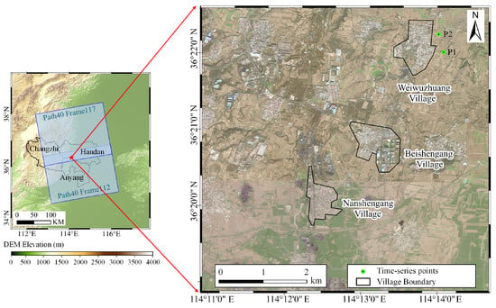
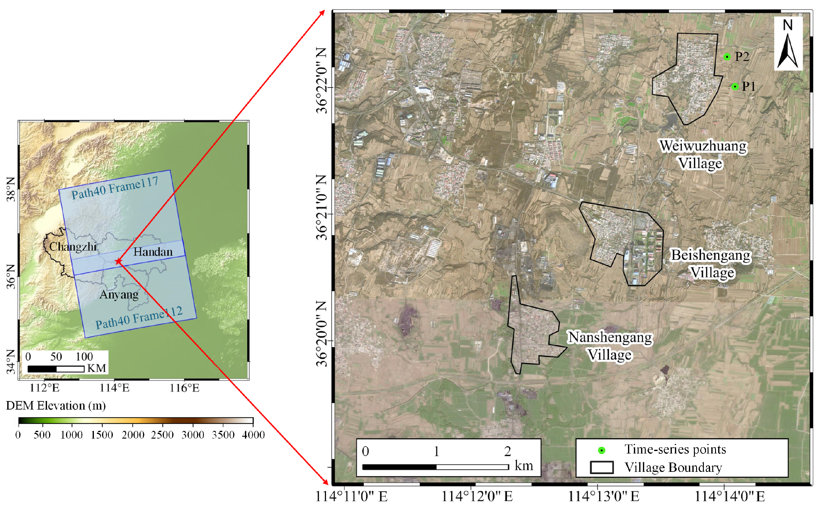
The study area is located in the Wutongzhuang Mine, Fengfeng Mining District, Handan City, Hebei Province, China, covering approximately and including Weiwuzhuang, Beishengang, and Nanshengang villages, as well as two leveling monitoring points, P1 and P2 [2] (Figure 1). The landscape transitions from low mountains and hills in the west to plains in the east. Land cover mainly consists of village buildings, farmland, and mining-related industrial land. Long-term underground coal mining activities in this area highlight the importance of surface deformation monitoring for village protection and mining safety [1,2].
Figure 1.
Study area.
The stratigraphic sequence of the Wutongzhuang Mine, from oldest to youngest, comprises the Ordovician Fengfeng Formation, Carboniferous Benxi and Taiyuan formations, Permian Shanxi, Lower Shihezi, and Upper Shihezi formations, Triassic Liujiagou Formation, and Cenozoic deposits. The Fengfeng Formation, consisting mainly of thick-bedded limestone and dolomitic limestone, forms the basement of the coal-bearing sequence. The Shanxi Formation is the principal coal-bearing unit, with a thickness of – (mean: ). The No. 2 coal seam is the main mining target, with a mean thickness of approximately . The Cenozoic cover ranges from to in thickness [2,34].
Overburden isolated grouting backfill technology was adopted at the 182211 and 182211N working faces of the Wutongzhuang Mine to mitigate mining-induced subsidence beneath villages [2,35]. This technology controls overburden deformation and its transmission to the surface through grouting and backfilling, providing an important approach to subsidence mitigation during coal extraction beneath villages [36]. Despite these mitigation measures, continuous monitoring of the spatial distribution and temporal evolution of surface deformation remains essential for assessing mining impacts and supporting mining safety management [1].
2.2. Sentinel-1 and Auxiliary Data
We used 276 ascending Sentinel-1 C-band SAR images for time-series surface deformation monitoring in the study area. The images cover the period from 10 January 2020 to 11 July 2024, with a nominal revisit interval of approximately 12 d. They were acquired on Path 40, Frames 112 and 117, in Interferometric Wide Swath (IW) mode with VV/VH dual polarization.
Auxiliary data included precise orbit products and the TanDEM-X Digital Elevation Model (DEM), used to improve orbital-parameter accuracy and remove topographic phase, respectively. A radar incidence angle of 0.6839 rad was used for vertical projection. The datasets and principal parameters used in this study are summarized in Table 1.
Table 1.
Sentinel-1 images and auxiliary data used in this study.
3. Methods
3.1. Overall Workflow
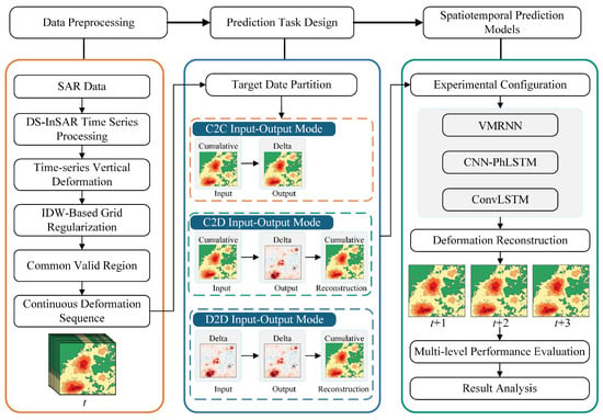
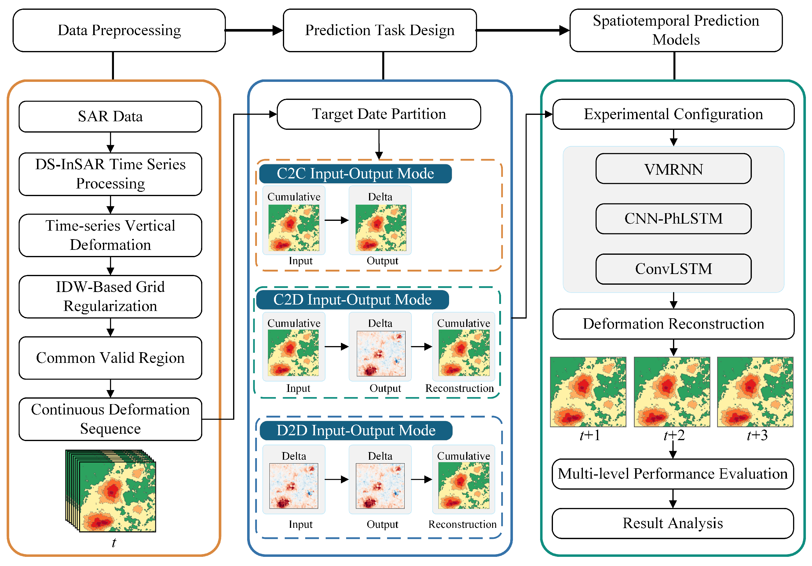
In this study, DS-InSAR was first applied to multi-temporal Sentinel-1 SAR images to monitor surface deformation and construct continuous two-dimensional cumulative vertical deformation fields. Three prediction tasks—namely, cumulative-input–cumulative-output (C2C), cumulative-input–increment-output (C2D), and increment-input–increment-output (D2D)—were then established. CNN-PhLSTM, ConvLSTM, and VMRNN were employed to predict short-term deformation evolution under the three tasks, and their predictive performance was evaluated using a unified evaluation procedure. The overall research framework is shown in Figure 2.
Figure 2.
Overall methodological framework of the study.
3.2. DS-InSAR Time-Series Deformation Processing
Distributed scatterer interferometric synthetic aperture radar (DS-InSAR) improves the spatial coverage of reliable measurements in time-series deformation monitoring by identifying statistically homogeneous pixels (SHPs) and optimizing the interferometric phases of distributed scatterers. The main processing steps include SHP identification, sample covariance matrix construction, phase estimation by eigenvalue decomposition, and subsequent time-series deformation inversion.
First, pixels with similar scattering statistics are identified using the amplitude time series of multitemporal SAR images. The Kolmogorov–Smirnov (KS) test is employed to compare the empirical cumulative distribution functions of the amplitude samples from a central pixel and its neighboring candidate pixels. Let and denote the empirical cumulative distribution functions of the amplitude samples of the central and candidate pixels, respectively. The KS statistic is defined as
Here, sup denotes the supremum. The KS test was conducted at a significance level of , using a search window of pixels (19 rows and 45 columns). The window extends 9 rows above and below and 22 columns to the left and right of the central pixel.
When the KS test yielded a p-value greater than 0.05, the null hypothesis that the amplitude samples of the two pixels followed the same distribution was not rejected. The candidate pixel was then included in the SHP set of the central pixel for subsequent covariance matrix estimation.
After SHP identification, the multitemporal complex-valued observations of the SHPs are used to construct a sample covariance matrix (SCM). Let N be the number of SAR acquisitions, L the number of looks used for statistical estimation, and the matrix of complex-valued observations. The SCM is expressed as
Here, consists of multitemporal complex-valued observation vectors for the L looks, and the superscript H denotes the conjugate transpose. By averaging the outer products of these observation vectors, the SCM characterizes the second-order statistical relationships among SAR acquisitions and provides the basis for subsequent phase estimation.
Temporal decorrelation and phase noise may introduce errors into the interferometric phases of distributed scatterers. To extract the dominant phase information, eigenvalue decomposition (EVD) is applied to the SCM:
Here, is the diagonal matrix of eigenvalues, is the matrix of corresponding eigenvectors, and and are the ith eigenvalue and eigenvector, respectively. In the conventional EVD approach, the principal eigenvector associated with the largest eigenvalue is selected to extract the dominant phase information from the SCM.
Let denote the eigenvector associated with the largest eigenvalue. Taking SAR acquisition r as the reference, the estimated relative phase for acquisition i is given by
Here, denotes the complex argument; and are the components of the principal eigenvector corresponding to acquisition i and the reference acquisition r, respectively; and the superscript ∗ denotes complex conjugation. The estimated phases are then used for the subsequent joint PS/DS time-series deformation inversion.
After time-series deformation inversion, assuming that vertical displacement dominates the surface motion in the mining area, line-of-sight (LOS) deformation is approximately projected into the vertical direction:
Here, and denote the LOS and vertical displacements, respectively.
Due to local decorrelation, DS-InSAR deformation measurements contain spatial gaps that limit their direct use in spatiotemporal prediction. Therefore, inverse distance weighting (IDW) interpolation was applied to estimate missing deformation values based on neighboring valid measurements. The distance-weighting power was set to 1.6, with a variable search neighborhood of the 10 nearest valid points.
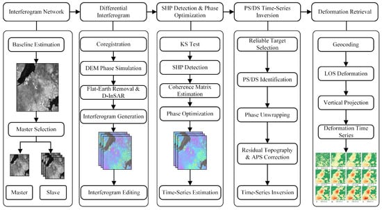
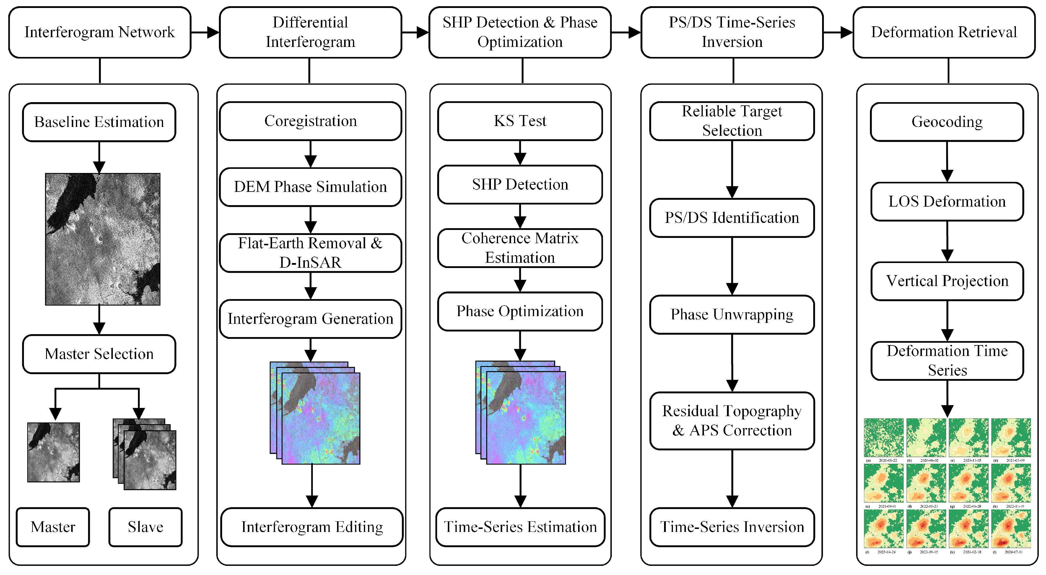
The deformation measurements were mapped onto a common grid, with an approximate spacing of 24 m in the east–west direction and 28 m in the north–south direction, yielding 138 cumulative two-dimensional vertical deformation fields. A common valid-pixel mask was defined by retaining pixels with finite values across all 138 epochs, resulting in 57,360 valid pixels. The overall DS-InSAR processing workflow is shown in Figure 3.
Figure 3.
DS-InSAR time-series deformation processing and construction of two-dimensional deformation fields.
3.3. Spatiotemporal Prediction Tasks and Models
3.3.1. Task Definition and Data Partitioning
The training, validation, and test sets were divided according to prediction target dates, and sliding prediction samples were constructed independently within each temporal interval. Each sample contains eight consecutive historical epochs and directly predicts the following three epochs, corresponding to lead times of approximately 12, 24, and 36 d. The training, validation, and test sets contain 99, 10, and 15 prediction windows, respectively. The corresponding target-date ranges are 15 April 2020 to 29 July 2023, 10 August 2023 to 20 December 2023, and 1 January 2024 to 11 July 2024.
Let denote the cumulative vertical deformation field at epoch t. The deformation increment between two adjacent epochs is defined as
The historical cumulative-deformation and deformation-increment sequences both have a length of eight. For the increment input, the first temporal position is initialized with a zero field, while the remaining seven positions contain differences between consecutive cumulative-deformation fields. The historical sequences are defined as
Here, denotes a zero-initialized placeholder rather than an observed zero deformation increment. This construction uses the same eight historical epochs across all three prediction tasks without requiring an additional cumulative field.
The future three-epoch cumulative-deformation supervision sequence and deformation-increment supervision sequence are, respectively, defined as
For each prediction task, the model takes the historical sequence as input and produces the future prediction , using the observed future sequence for supervision. The corresponding task configurations are summarized in Table 2.
Table 2.
Definitions of the C2C, C2D, and D2D spatiotemporal prediction tasks.
3.3.2. Spatiotemporal Models for Two-Dimensional Mining Deformation Prediction
Under the unified task definition, CNN-PhLSTM [24], ConvLSTM [23], and VMRNN [26] were selected as the three spatiotemporal prediction models. Each model was applied to the C2C, C2D, and D2D tasks, forming a unified cross-task and cross-network comparison matrix.
CNN-PhLSTM uses a convolutional encoder to extract two-dimensional spatial features and Peephole LSTM to characterize temporal evolution across consecutive epochs [24]. ConvLSTM embeds convolution operations into recurrent-state updates to preserve two-dimensional spatial structure during temporal information propagation [23]. VMRNN combines visual state-space modeling with recurrent memory to jointly represent two-dimensional spatial context and continuous temporal states [26]. To reduce the effect of differences in model size, the number of trainable parameters in all three networks was controlled at approximately 1 M. The main architectures and configurations are summarized in Table 3.
Table 3.
Architectural configurations and parameter sizes of the three spatiotemporal prediction models.
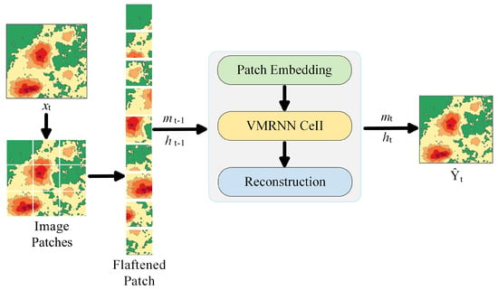
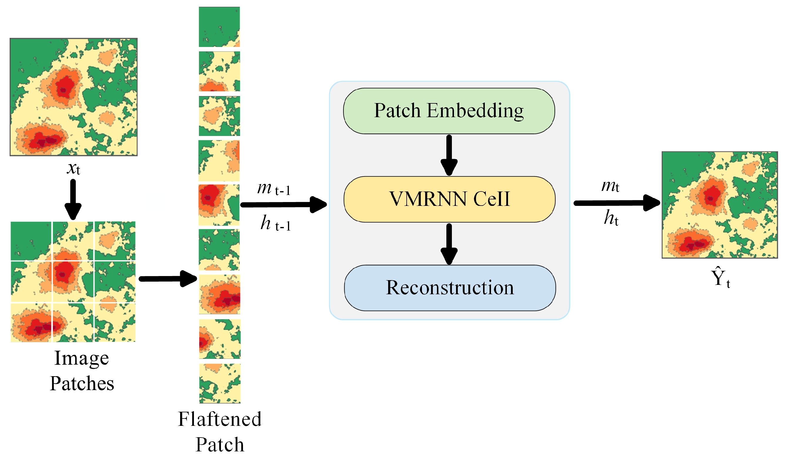
Among the three models, VMRNN adopts the VMRNN-B configuration proposed by Tang et al. [26], and its overall prediction architecture is shown in Figure 4. For each epoch in the historical input sequence, the current single-epoch deformation field is first partitioned into image patches and encoded into features. Let denote the single-epoch feature obtained by the encoder at epoch t. The hidden state and memory state from the previous epoch are denoted by and , respectively. The VMRNN Cell combines the current input feature with the historical states to extract spatial features and update the temporal states, yielding the current hidden state and memory state . After all eight historical epochs have been sequentially processed by the recurrent unit, the decoder directly generates the three-epoch future prediction sequence .
Figure 4.
VMRNN architecture for direct multi-step prediction.
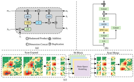
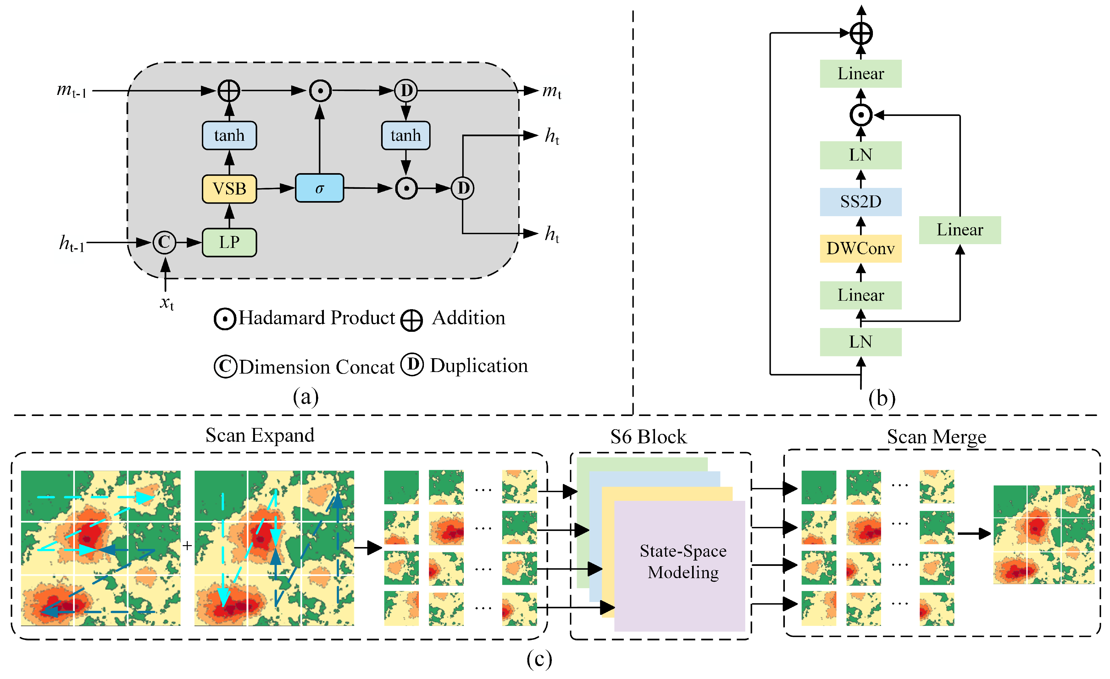
The VMRNN cell mainly consists of a visual state-space block (VSS block) and a recurrent-state update module, as shown in Figure 5. The current single-epoch feature and the hidden state from the previous epoch are first concatenated along the feature dimension. A linear projection and VSS block are then applied to obtain the current spatiotemporal feature :
Figure 5.
Core modules of VMRNN, redrawn based on the architecture proposed by Tang et al. [26]. (a) VMRNN cell; (b) VSS block; (c) SS2D.
The two-dimensional selective scan module (2D selective scan, SS2D) within the VSS Block unfolds the two-dimensional features along multiple spatial directions and applies the S6 state-space model to the resulting sequences. The outputs from the different directions are subsequently restored and merged into the original two-dimensional space, thereby establishing contextual relationships among different spatial locations within each epoch.
Along the temporal dimension, and propagate information across consecutive epochs. A gating variable is generated from the current spatiotemporal feature as
The memory state is then updated as
and the hidden state is updated as
Through these state updates, the spatial features extracted at the current epoch and the historical states are progressively propagated along the temporal sequence and used for feature modeling at subsequent epochs.
For different task configurations, only the deformation representations of the historical input and future supervision target are changed, while the main network architecture remains unchanged. The principal structural configurations of the three models are summarized in Table 3.
3.3.3. Model Training and Reconstruction of Cumulative Deformation
Before model training, the cumulative vertical deformation fields were standardized using Z-score normalization based on statistics from the training set:
Here, and are the mean and standard deviation, respectively, of cumulative vertical deformation over all valid pixels in the training period. The normalization parameters determined from the training set were fixed and subsequently applied to the validation and test sets.
All three prediction tasks were optimized using masked mean squared error (masked MSE) within their respective supervision-target spaces:
Here, is the valid-pixel indicator, and N is the number of scalar positions in the supervision-target tensor.
For C2C, the predicted standardized fields are transformed back to the cumulative-deformation space as follows:
For C2D and D2D, the predicted standardized increments, obtained from differences between standardized cumulative fields, are rescaled and accumulated from the last observed field to reconstruct future cumulative deformation:
Here, corresponds to the 12, 24, and 36 d lead times. All three tasks are evaluated in the reconstructed cumulative-deformation space.
All three networks were trained using the AdamW optimizer with a base learning rate of , a weight decay coefficient of , a batch size of 1, gradient clipping at 1.0, and a maximum of 400 epochs. The first five epochs used learning-rate warm-up, followed by cosine annealing with a minimum learning rate of . These training settings were shared across all nine network–task combinations.
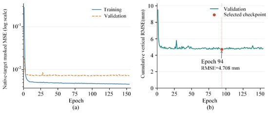
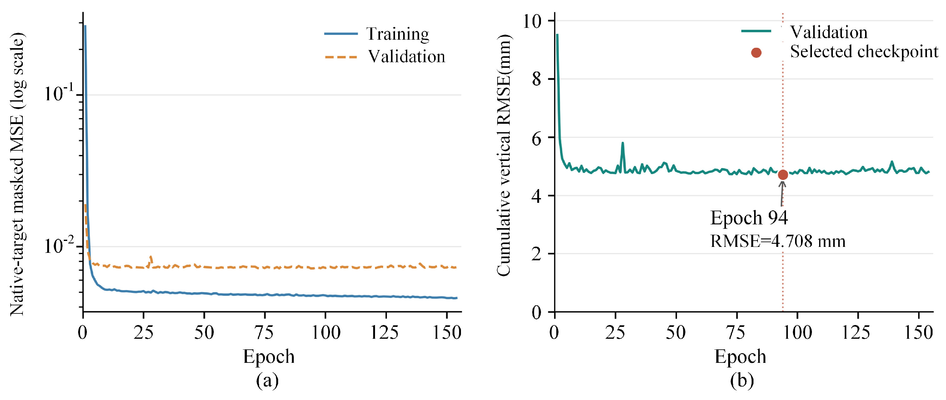
During training, the best checkpoint was updated from the first epoch based on validation RMSE in the reconstructed cumulative-deformation space. Early-stopping patience counting was enabled from epoch 50, with a patience of 60 epochs without sufficient improvement. This setting allowed an initial optimization period without excluding checkpoints obtained before epoch 50.
Each of the nine network–task combinations was trained with three independent random seeds (2025, 2026, and 2027), yielding 27 experiments under identical data partitions and training settings. Figure 6 illustrates the representative VMRNN-D2D training and model selection process using seed 2025.
Figure 6.
VMRNN-D2D training and model selection process. (a) Training and validation masked MSE; (b) validation cumulative-deformation RMSE.
3.3.4. Evaluation Metrics and Persistence Baselines
All predictions were evaluated in the original cumulative vertical deformation space. Root mean square error (RMSE), mean absolute error (MAE), the coefficient of determination , and the structural similarity index measure (SSIM) [37] were used as the overall evaluation metrics.
RMSE is defined as
MAE is defined as
The coefficient of determination is defined as
For a two-dimensional cumulative deformation field C and its predicted field , and are constants introduced for numerical stability. The structural similarity index measure (SSIM) is defined as follows:
For each random seed, the overall evaluation included 15 test windows and 3 lead times (12, 24, and 36 d), yielding 45 predicted deformation fields. RMSE, MAE, and were computed by pooling all valid pixels across these fields, whereas SSIM was calculated for each field and then averaged. Predictions for the same target date from different forecast origins or lead times were counted separately. The metrics were reported as the mean and sample standard deviation across three random seeds.
The valid samples were further classified by deformation intensity using the 50th and 95th percentiles ( and ) of cumulative subsidence magnitude in the training set, as defined below:
The stratification thresholds determined from the training set were and .
RMSE was calculated separately for the three deformation intensity classes, and the contribution of each class to the total squared error was calculated as
Here, .
The global peak bias was computed for each random seed by pooling all valid pixels across test windows and prediction lead times:
Here, denotes the set of valid pixel–forecast-instance triples, where w, k, and i index the test window, prediction lead time, and grid pixel, respectively.
In addition, two training-free persistence baselines, zero persistence and last-delta, were used to evaluate whether the deep learning models could improve upon simple temporal persistence and linear extrapolation strategies. Zero persistence retains the cumulative deformation at the final epoch of the input window:
Last-delta linearly extrapolates the most recent deformation increment:
4. Results
4.1. InSAR Monitoring Consistency Validation and Spatiotemporal Evolution
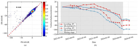
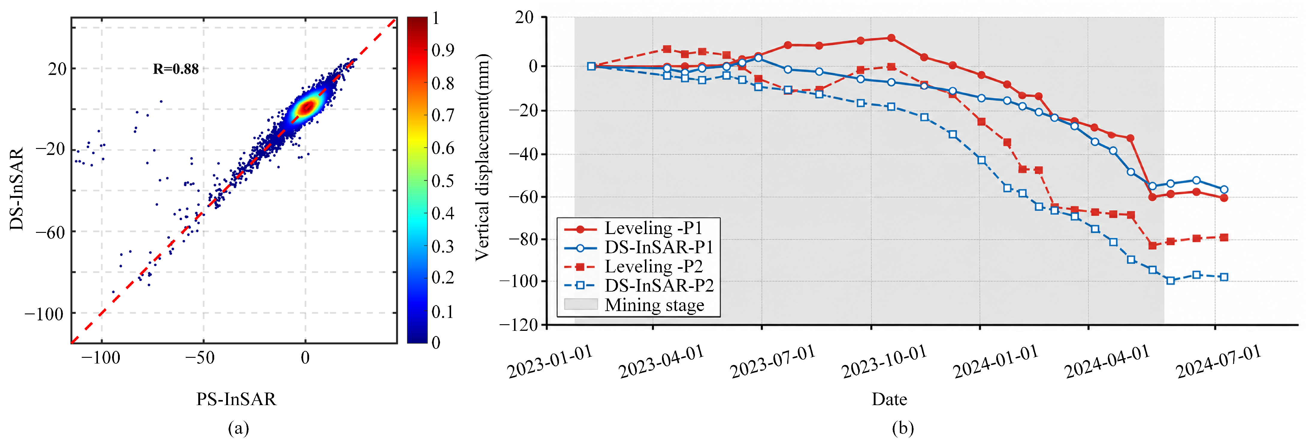
To assess the reliability of the InSAR deformation results, we first matched spatially corresponding PS-InSAR and DS-InSAR measurement points within the study area during 2022–2023, using a search radius of 20 m. The Pearson correlation coefficient between their deformation rates was 0.88, indicating a high level of consistency (Figure 7a).
Figure 7.
(a) Colocated PS-InSAR and DS-InSAR deformation rates; (b) comparisons of cumulative vertical displacement derived from DS-InSAR and leveling at P1 and P2.
Furthermore, the contemporaneous leveling observations at P1 and P2 from February 2023 to July 2024 were used to validate the vertical deformation derived from DS-InSAR [2]. The comparison yielded a Pearson correlation coefficient of , , MAE = , and RMSE = (Figure 7b). The subsidence trends at the two leveling points closely agreed with the DS-InSAR monitoring results, indicating the high reliability of the InSAR deformation retrievals and the reasonableness of the experimental parameter settings in this study.
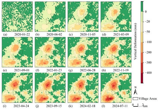
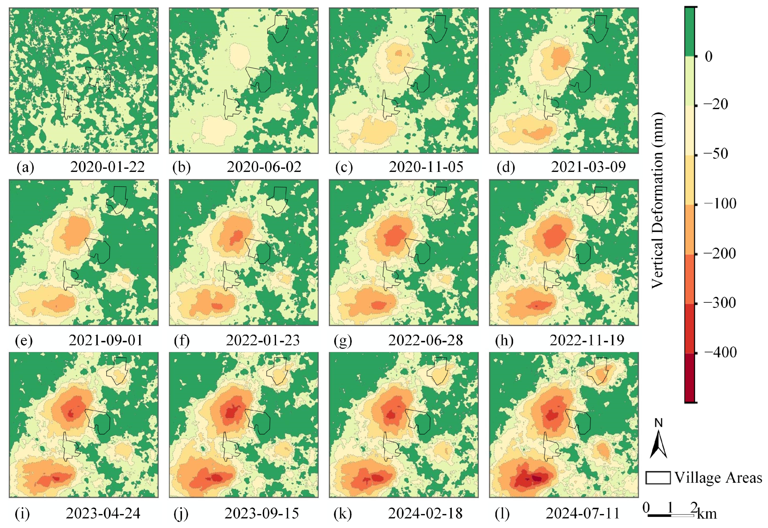
Figure 8 shows the cumulative vertical deformation fields at 12 representative epochs from 10 January 2020 to 11 July 2024. Overall, two major subsidence zones gradually developed in the north-central and southwestern parts of the study area. Once established, their spatial patterns remained relatively stable, while subsequent evolution was mainly characterized by continued increases in subsidence magnitude and further expansion of the affected areas. The maximum cumulative vertical deformation during the study period was approximately .
Figure 8.
Evolution of cumulative vertical deformation in the Wutongzhuang Mine at representative epochs.
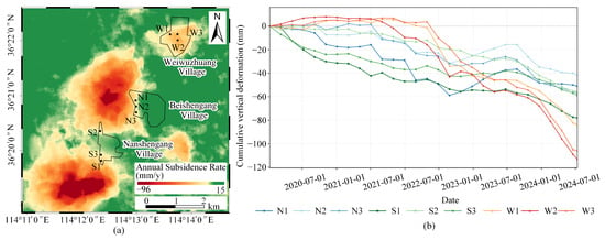
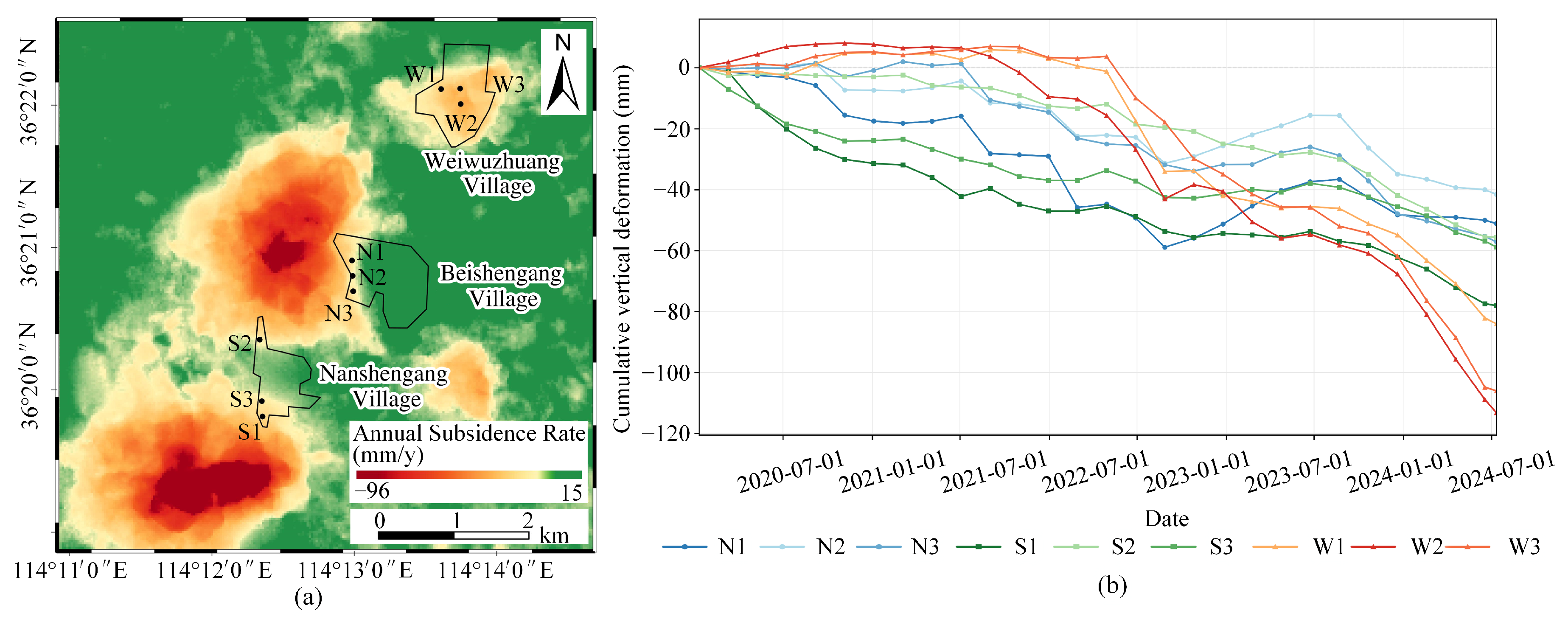
As shown in Figure 9, three representative sampling points were selected near the deformation-affected areas of each of Weiwuzhuang Village, Beishengang Village, and Nanshengang Village to analyze their historical cumulative vertical deformation.
Figure 9.
(a) Annual average subsidence rate and spatial locations of the sampling points; (b) historical cumulative vertical deformation at the sampling points.
Weiwuzhuang Village exhibited relatively small deformation during 2020–2021, followed by a marked increase in subsidence from 2022 onward. During the same period, the 182211 and 182211N working faces of the Wutongzhuang Mine were mined beneath village areas, with overburden isolated grouting employed to control surface subsidence [36]. The increased subsidence in Weiwuzhuang Village broadly coincided with the mining periods of these working faces, suggesting a possible influence from nearby mining activities. The mean cumulative vertical deformation of its representative points increased from approximately at the end of 2021 to at the end of 2022, reaching on 11 July 2024.
Beishengang Village is located in the central part of the Wutongzhuang mining field, where deformation rates within the village were generally low. However, its western side, adjacent to the margin of the north-central subsidence trough, exhibited relatively pronounced negative deformation. The mean cumulative vertical deformation of its representative points evolved from approximately at the end of 2020 to at the end of the study period, with some stage-dependent fluctuations.
Nanshengang Village is situated between the north-central and southwestern subsidence zones and exhibited noticeable cumulative subsidence during the early study period. The mean cumulative vertical deformation of its representative points gradually increased from approximately at the end of 2020 to at the end of the study period.
The three villages thus exhibited distinct differences in cumulative deformation magnitude, the timing of subsidence development, and subsequent deformation evolution.
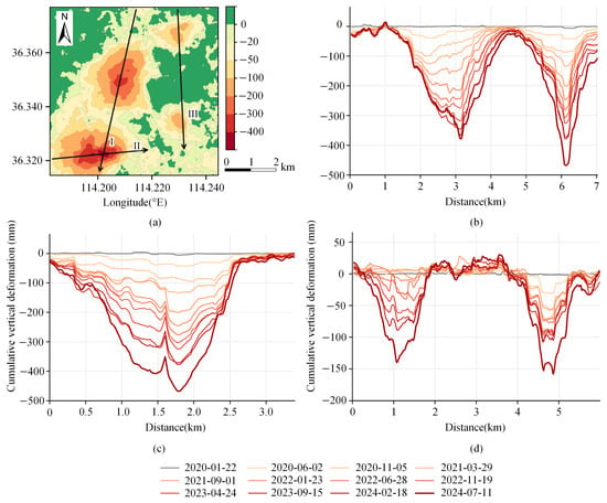
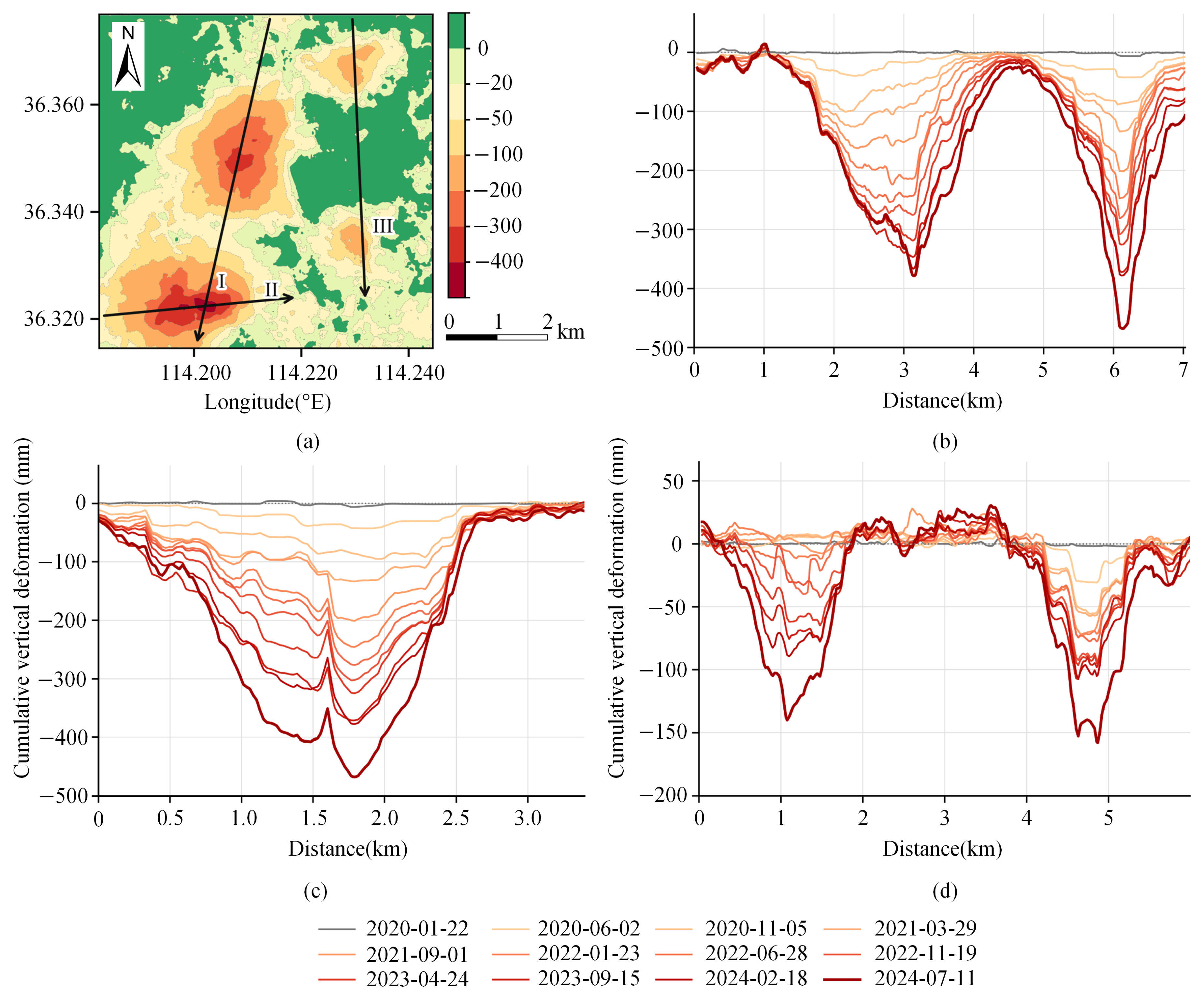
To further analyze the evolution of surface deformation in the major subsidence zones, cumulative vertical deformation profiles at different epochs were extracted along Profiles I, II, and III, as shown in Figure 10.
Figure 10.
Evolution of cumulative vertical deformation along representative profiles in the Wutongzhuang Mine. (a) 2024-07-11: fixed profiles; (b) Profile I; (c) Profile II; (d) Profile III.
Profile I crosses both the southwestern and north-central major subsidence zones and exhibits two distinct subsidence troughs corresponding to the two principal subsidence centers. Along the north-to-south direction, the deformation profiles of the two major subsidence zones exhibit distinct trough-shaped patterns that are qualitatively similar to classical settlement-trough profiles. Profile II crosses the southwestern subsidence zone, where the largest deformation magnitude was observed, with a maximum negative displacement of approximately .
Profile III illustrates the evolution of two local subsidence troughs in the eastern part of the study area. Both troughs exhibited continued deepening during the later study period, with a maximum negative displacement of approximately .
As shown in Figure 10b–d, the cumulative subsidence curves from 2020 to 2023 generally exhibited relatively similar spacing between successive epochs, indicating comparatively stable subsidence development during this period. In 2024, the spacing between successive curves increased noticeably in some subsidence troughs, indicating an increase in local subsidence rates during the later study period.
4.2. Comparison of Prediction Tasks and Model Performance
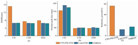
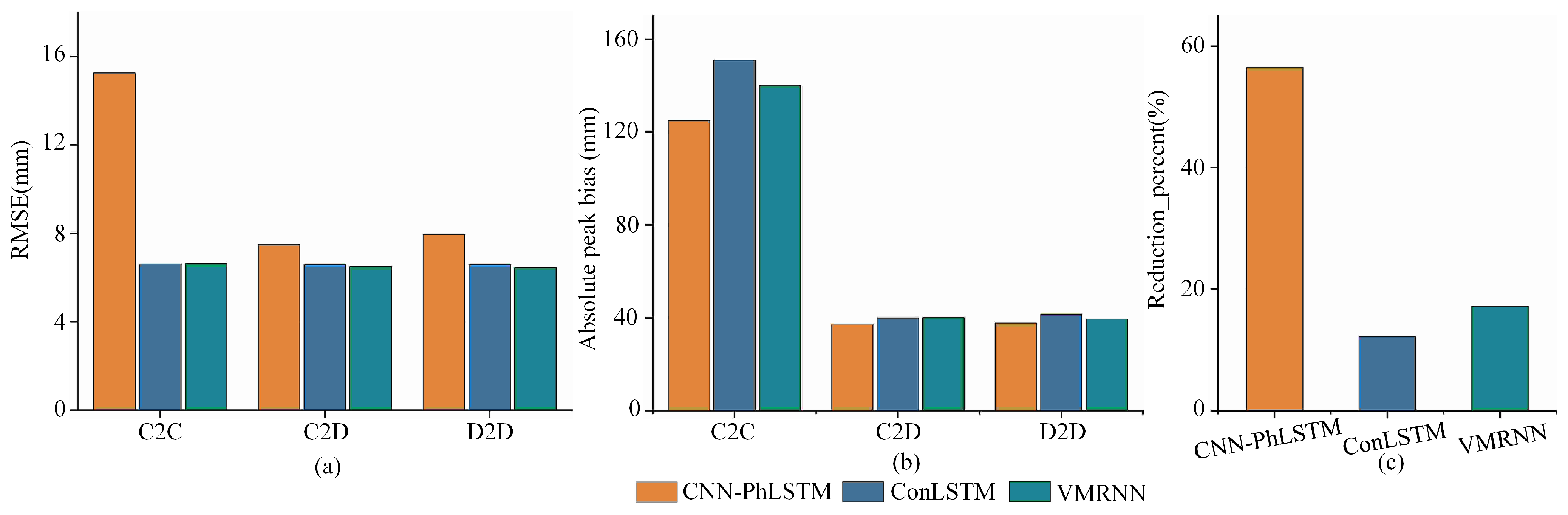
To evaluate the effect of increment-based future supervision, we compared seed-wise relative RMSE reductions from C2C to C2D (Table 4). With the historical cumulative deformation input held unchanged, converting only the future supervision targets to deformation increments reduced prediction errors for all three networks. The mean RMSE reduction was largest for CNN-PhLSTM (56.48%), followed by VMRNN (17.16%) and ConvLSTM (12.17%). The direction of improvement was consistent across three random seeds for each network (Figure 11c). In contrast, converting C2D to D2D produced substantially smaller performance changes, as shown in Figure 11a. VMRNN achieved the largest mean RMSE reduction of 2.27%, whereas CNN-PhLSTM exhibited a slight increase in RMSE. Thus, further converting the historical input to deformation increments had a smaller and model-dependent effect than converting the future supervision target to increments. Task configuration also affected the recovery of strong-subsidence magnitudes. As shown in Figure 11b, the absolute peak bias decreased markedly for all three networks from C2C to D2D. For ConvLSTM, the peak bias changed from to , representing a reduction of in absolute peak bias. These results indicate that task representation affects not only overall RMSE but also the recovery of strong-subsidence magnitudes.
Table 4.
Performance of the three models under the C2C, C2D, and D2D tasks.
Figure 11.
Prediction performance of the three models under different task configurations. (a) Overall error; (b) peak recovery; (c) C2C to C2D gain.
To further compare network architectures under a unified prediction task, we evaluated CNN-PhLSTM, ConvLSTM, and VMRNN under D2D, together with zero persistence and last-delta as persistence baselines. As shown in Table 5, the three deep learning models achieved relatively similar overall predictive performance. VMRNN obtained the lowest mean RMSE and MAE of and , respectively, as well as the highest mean of . ConvLSTM achieved the highest mean SSIM of . Compared with zero persistence, the RMSE of VMRNN-D2D decreased from 6.647 mm to 6.440 mm, corresponding to an improvement of approximately 3.1%.
Table 5.
Overall performance under the D2D task.
Table 6 further presents the performance of the D2D task at lead times of 12, 24, and 36 d. As the forecast horizon increased, the RMSEs of all three deep learning networks increased, while spatial structural similarity generally decreased. Among the three deep learning networks, VMRNN achieved the lowest mean RMSE at each lead time, including 4.741 mm at 12 d; ConvLSTM achieved the highest mean SSIM at each lead time. Therefore, VMRNN-D2D demonstrates a certain advantage in controlling overall prediction errors, motivating the following analysis of its short-term deformation prediction characteristics.
Table 6.
Performance at different lead times under the D2D task.
4.3. Short-Term Deformation Prediction Characteristics of VMRNN-D2D
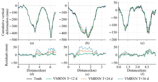
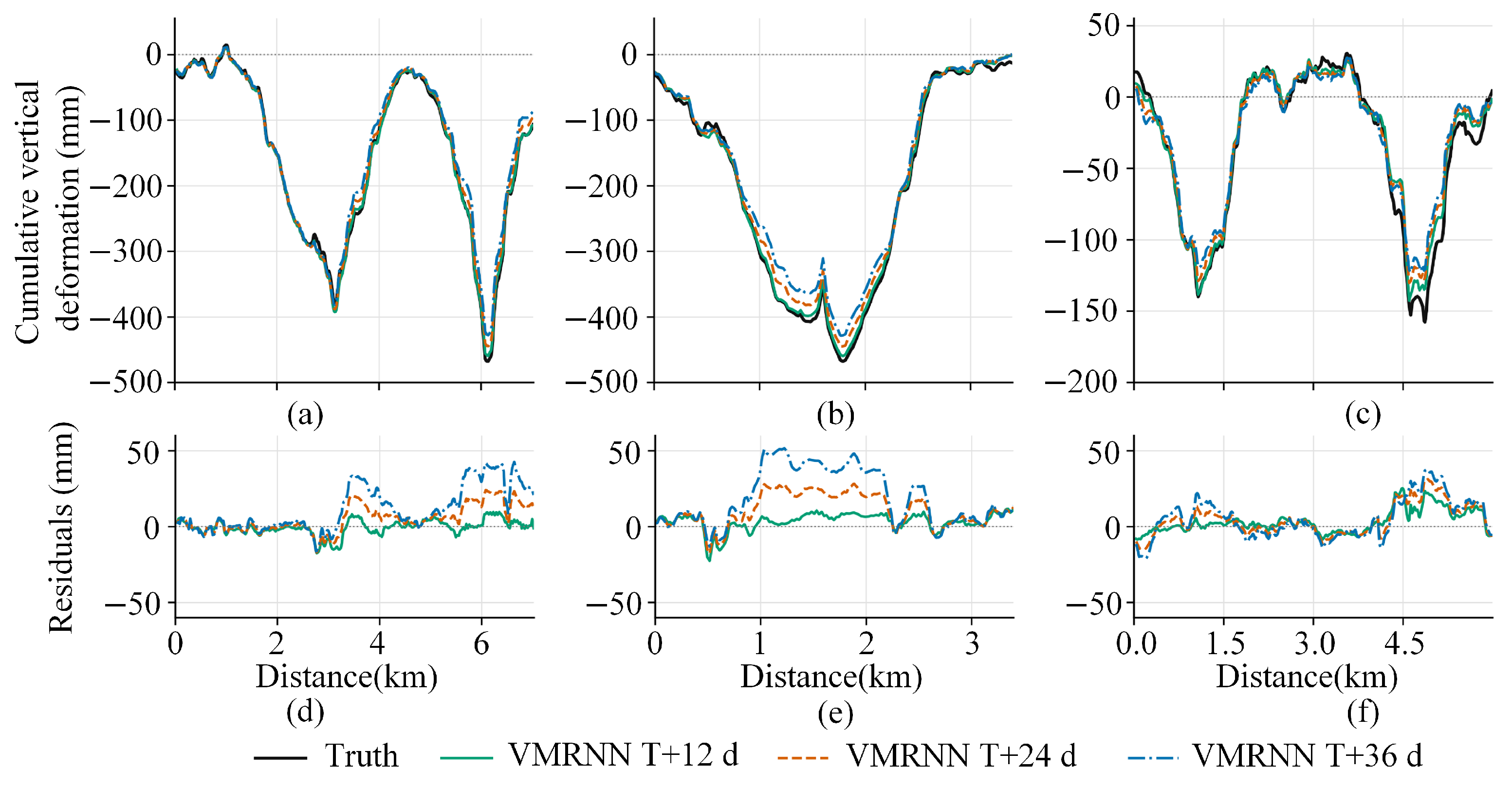
To evaluate the ability of VMRNN-D2D to reconstruct cumulative deformation at different short-term lead times and maintain consistency across subsequent prediction visualizations, we used the model trained with random seed 2025 to compare predictions at 12, 24, and 36 d against the observed cumulative vertical deformation on the common target date of 11 July 2024, using the three fixed profiles defined in Figure 10. Residuals are defined as predicted minus observed cumulative deformation. For subsiding areas, positive residuals indicate underestimation of subsidence magnitude, whereas negative residuals indicate overestimation.
As shown in Figure 12, the VMRNN-D2D prediction curves captured the main deformation characteristics of the observed profiles at all three lead times. The 12 d predictions were closest to the observations. As the lead time increased to 24 and 36 d, magnitude discrepancies at the subsidence trough bottoms and adjacent high-gradient sections became progressively larger. The residuals were mainly concentrated in local sections with large subsidence magnitudes, with the smallest overall residuals observed at 12 d.
Figure 12.
Fixed-profile predictions and residuals of VMRNN-D2D at different lead times. (a) Profile I; (b) Profile II; (c) Profile III; (d) Profile I: residuals; (e) Profile II: residuals; (f) Profile III: residuals.
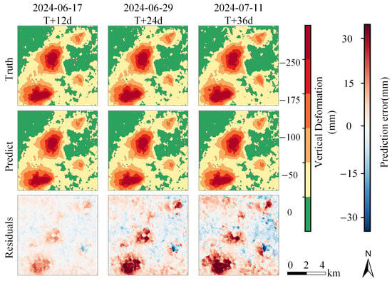
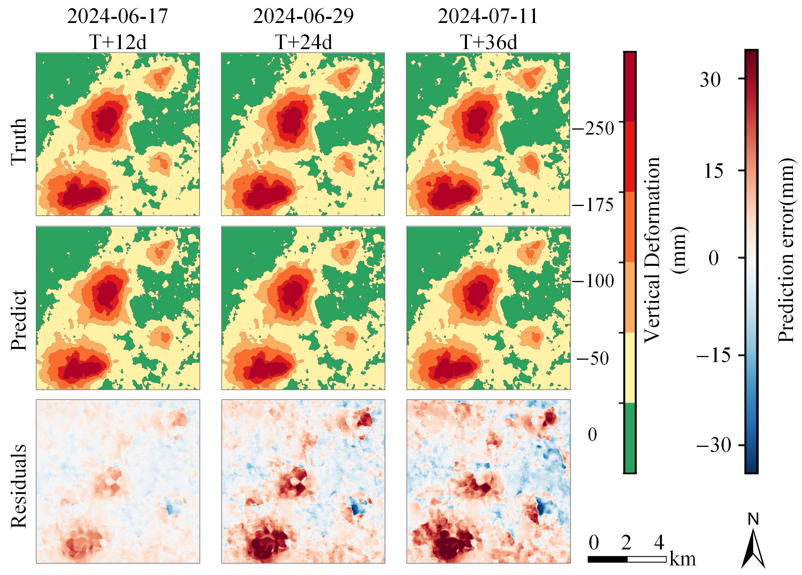
To further examine the ability of VMRNN-D2D to track future deformation evolution at the two-dimensional spatial scale, we used the same prediction origin to compare observed cumulative vertical deformation fields, predictions, and residual fields at 12, 24, and 36 d. As shown in Figure 13, the predicted locations and overall spatial outlines of the two major subsidence zones in the north-central and southwestern parts of the study area were consistent with the observations. As the lead time increased, the differences between predicted and observed fields gradually became larger. The most pronounced residuals were mainly distributed around the two major subsidence centers and adjacent areas with large deformation gradients, indicating that the model tended to underestimate subsidence magnitudes in actively developing strong-subsidence regions. Overall, VMRNN-D2D consistently preserved the principal spatial subsidence patterns at different lead times, while the increased errors at longer lead times were mainly associated with the recovery of local strong-subsidence magnitudes.
Figure 13.
Predictions and residuals of VMRNN-D2D for the final test window.
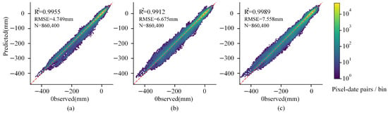
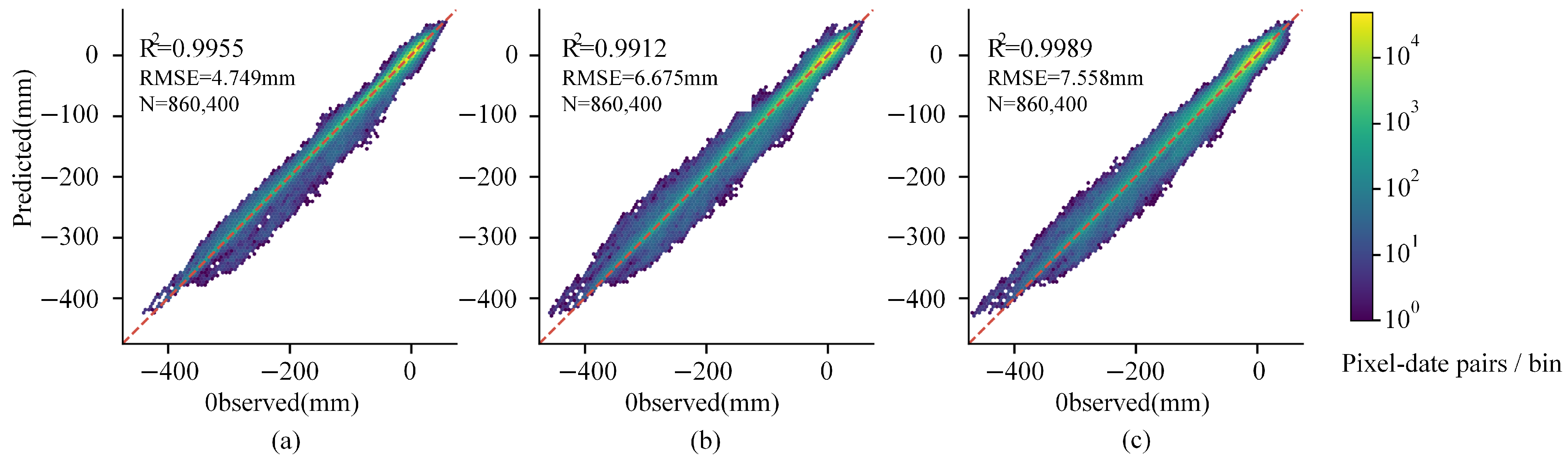
Figure 14 aggregates all valid pixels from the 15 test windows at each lead time and presents the hexagonal density distributions of predicted versus observed values. At the 12, 24, and 36 d lead times, the values exceeded 0.98 and the RMSEs remained below 7.6 mm. At all three lead times, most pixels were concentrated near the 1:1 reference line, indicating overall agreement between predictions and observations throughout the test period. As the lead time increased, the point cloud became progressively more dispersed around the 1:1 line. The most pronounced deviations occurred at large negative deformation magnitudes, where predicted values were generally closer to zero, indicating that prediction errors at longer lead times remained concentrated in regions with large subsidence magnitudes.
Figure 14.
Pixel density distributions of predicted versus observed values for VMRNN-D2D at different lead times. (a) 12 d; (b) 24 d; (c) 36 d.
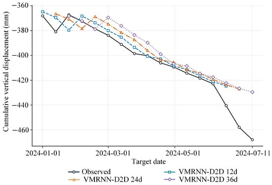
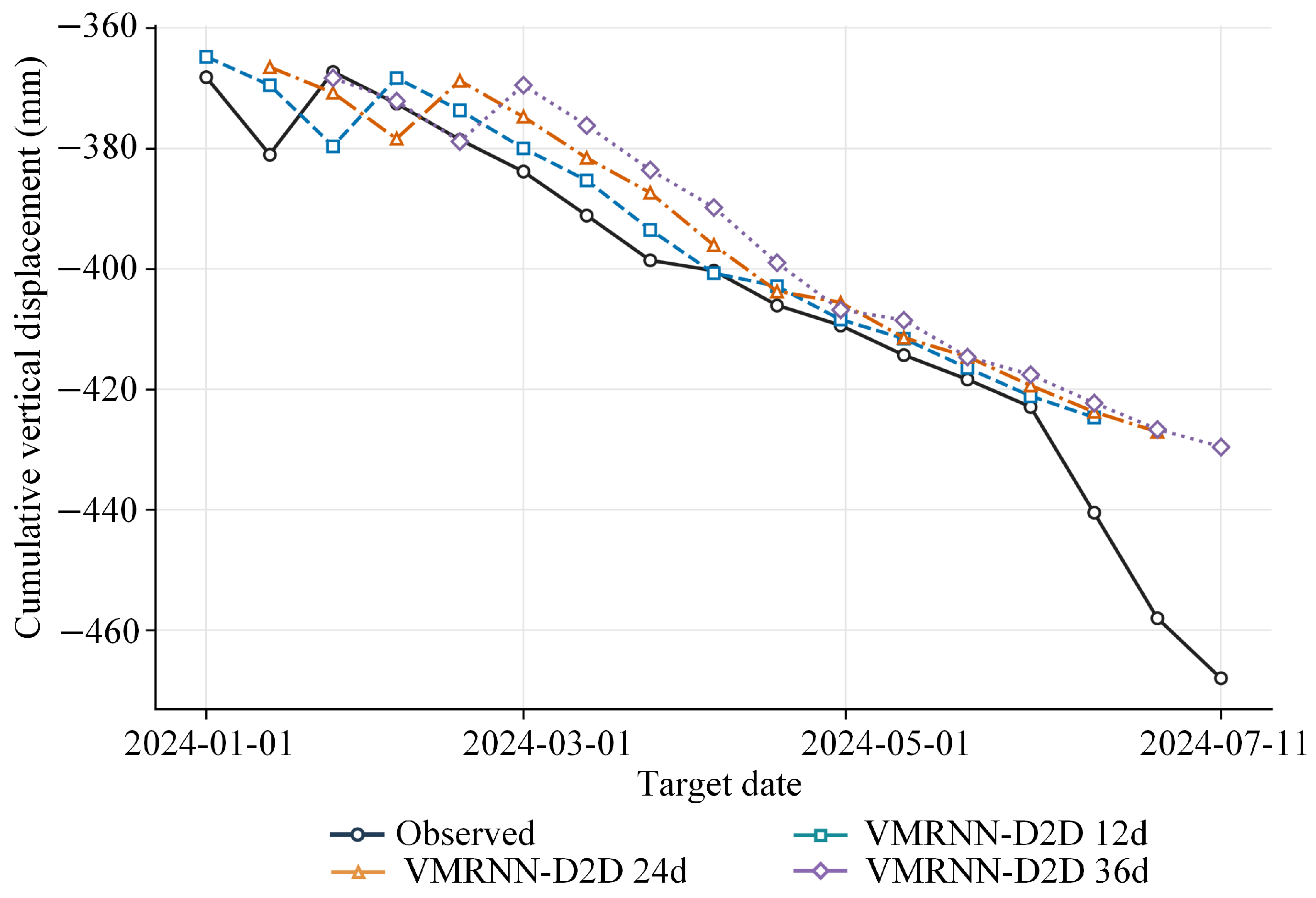
The evolution of maximum cumulative subsidence with target date during the test period provides further information on the model’s ability to track strong-subsidence development, as shown in Figure 15. From March to May 2024, predictions at different lead times followed trends similar to the observed maximum cumulative subsidence. After June, the observed maximum cumulative subsidence began to deepen markedly, whereas predictions at different lead times continued to vary more gradually, causing the discrepancy between predicted and observed values to increase rapidly. By 11 July 2024, the observed maximum cumulative vertical deformation reached , while the corresponding 36 d prediction was . This indicates that the model can effectively track the overall trend of maximum cumulative subsidence but responds less strongly to the accelerated deepening observed during the later part of the study period.
Figure 15.
Evolution of maximum cumulative subsidence with target date for VMRNN-D2D at different lead times during the test period.
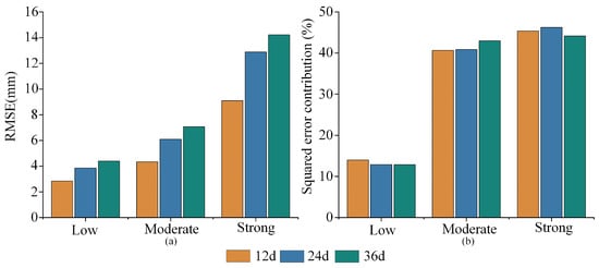
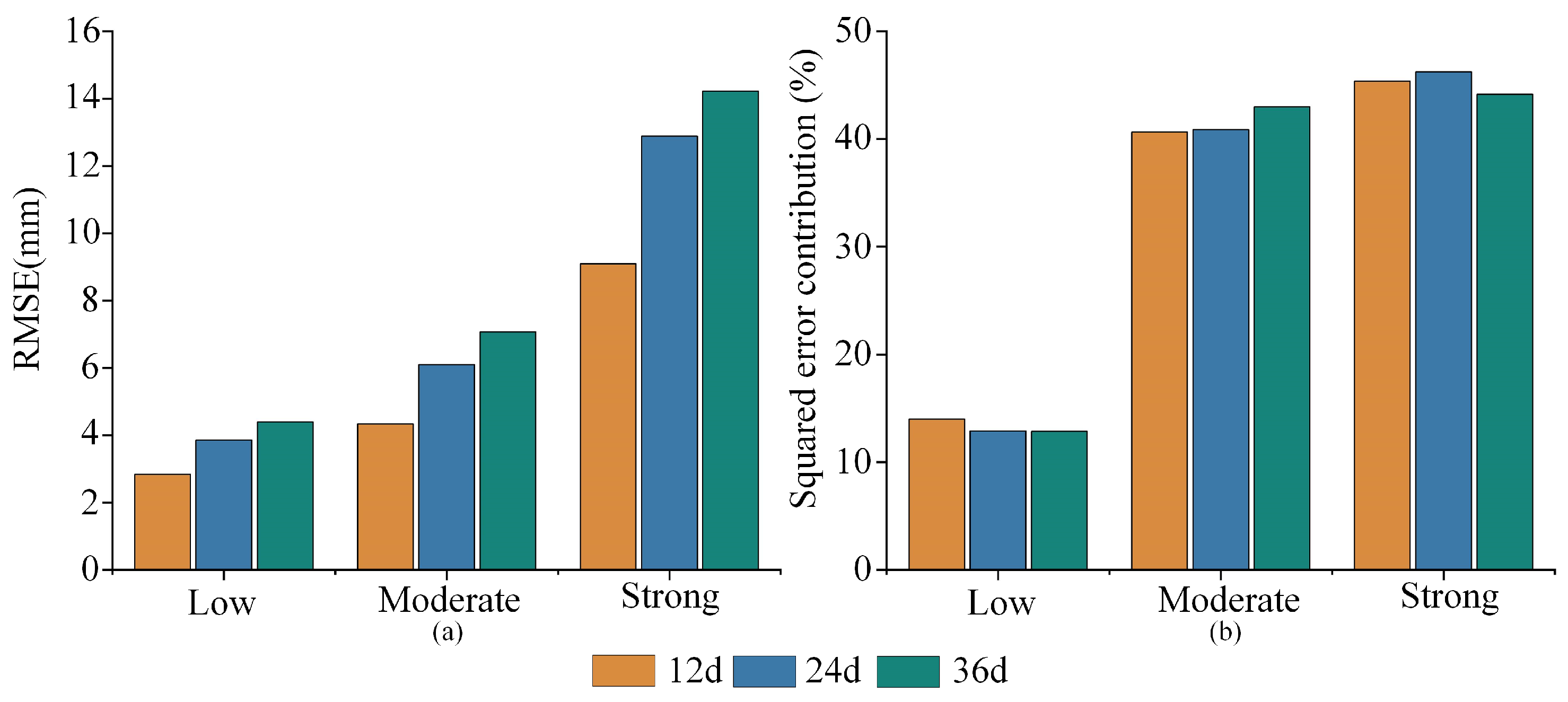
To further quantify the relationship between prediction errors and deformation intensity while reducing the influence of random initialization on the evaluation, we classified the test pixels into three deformation intensity categories—namely Low, Moderate, and Strong—using thresholds derived from cumulative subsidence magnitudes in the training set. The stratified evaluation metrics were calculated separately for the three random seeds and then averaged. As shown in Figure 16a, RMSE increased with deformation intensity at all three lead times. The RMSEs for the Strong category were 9.095, 12.882, and 14.221 mm at the 12, 24, and 36 d lead times, respectively, substantially higher than those of the corresponding Low and Moderate categories. The contributions of different deformation intensity categories to the total squared error also varied considerably. As shown in Figure 16b, the Strong category accounted for only approximately 12.3–12.5% of valid test pixels but contributed 44.16–46.24% of the total squared error. In contrast, the Low category represented approximately 38–39% of valid pixels but contributed only 12.9–14.0% of the total squared error. These results indicate a close relationship between prediction errors and deformation intensity, with the largest share of total squared error concentrated in the Strong category.
Figure 16.
Error groups for strong, moderate, and low subsidence: (a) RMSE (mm); (b) squared error contribution (%).
Overall, VMRNN-D2D consistently preserved the principal spatial structure of subsidence within the 12–36 d short-term prediction range, while the remaining errors were concentrated mainly in the recovery of subsidence magnitudes within Strong regions at longer lead times.
5. Discussion
5.1. Increment-Based Supervision Targets and Model Prediction Performance
This study systematically examined how deformation representation affects short-term prediction performance by comparing CNN-PhLSTM, ConvLSTM, and VMRNN under C2C, C2D, and D2D tasks. The results show that changing the future supervision targets from cumulative deformation to deformation increments consistently reduced prediction errors across all three networks. In contrast, further converting the historical inputs to increments produced relatively small, model-dependent benefits. This indicates that future-target representation is an important factor affecting short-term deformation prediction performance.
Cumulative deformation fields contain substantial historical subsidence information, and the spatial outlines of the major subsidence areas exhibit pronounced short-term persistence. Increment-based supervision encourages the model to focus more directly on deformation newly occurring during the prediction horizon. Under the unified D2D task, VMRNN showed advantages in RMSE, MAE, and and generally preserved the spatial structures of major subsidence funnels, reflecting its ability to model spatiotemporal features of two-dimensional deformation fields. Overall, this study demonstrates that increment-based supervision can effectively improve short-term deformation prediction across different networks and provide useful information for the analysis of spatiotemporal subsidence evolution and identification of key deformation areas.
5.2. Limitations and Future Research Directions
Although VMRNN-D2D generally preserved the spatial structures of major subsidence funnels, it still underestimated subsidence magnitudes in continuously developing strong-subsidence areas. During the later study period, deformation rates accelerated in some areas, whereas the predictions changed more gradually, indicating that models relying only on historical deformation sequences have limited ability to respond to rapidly changing deformation. Future work could introduce external driving information, such as working-face locations and mining progress, to improve predictions of rapidly developing subsidence.
Furthermore, this study used only ascending-orbit SAR data and converted line-of-sight (LOS) displacement to vertical displacement under the assumption that vertical motion dominates. Previous research has shown that neglecting horizontal motion can produce spatially structured errors in vertical deformation estimates and affect local deformation magnitudes and spatial patterns near subsidence boundaries. The conversion results in this study may therefore also be affected by this factor (Ma et al. [38]).
Future work could further explore tiered early-warning methods based on predicted deformation increments, deformation rates, and validated risk thresholds, together with risk verification using mining plans and on-site measurements, to better support continuous monitoring and safe management of surface subsidence in mining areas.
6. Conclusions
We used Sentinel-1 time-series SAR data and DS-InSAR to construct continuous two-dimensional cumulative vertical deformation fields for the Wutongzhuang Mine and performed short-term predictions at 12–36 d lead times. Monitoring showed that, after the two major subsidence zones formed, their locations and basic spatial outlines remained generally stable, while subsequent changes were characterized mainly by increasing subsidence magnitudes and expansion of the affected areas. The colocated PS-InSAR and DS-InSAR deformation rates had a correlation of 0.88; DS-InSAR and leveling observations at P1 and P2 yielded a correlation of 0.9742, an MAE of 8.23 mm, and an RMSE of 10.29 mm, indicating high consistency between InSAR monitoring results and independent ground measurements.
On this basis, we established C2C, C2D, and D2D prediction tasks for CNN-PhLSTM, ConvLSTM, and VMRNN to compare the effects of future supervision target representation and historical input representation on short-term cumulative deformation prediction. Keeping the historical cumulative deformation inputs unchanged and converting only the future targets to increments consistently reduced prediction errors for all three networks, whereas further converting the historical inputs to increments produced smaller, model-dependent benefits.
Under the unified D2D task, the three networks achieved broadly similar overall performance. VMRNN obtained the lowest mean RMSE and MAE and the highest mean , whereas ConvLSTM obtained the highest mean SSIM; overall, VMRNN-D2D showed relatively favorable predictive performance among the compared configurations. Analyses at different spatial scales showed that VMRNN-D2D generally preserved major subsidence zones and local trough structures but tended to underestimate deformation magnitudes in actively developing strong-subsidence areas. In summary, for cumulative InSAR deformation with pronounced short-term persistence, increment-based future supervision enables the model to focus more directly on deformation newly occurring during the prediction horizon and was the most consistent source of performance improvements across networks in this study.
Author Contributions
Conceptualization, S.L. (Simeng Luo) and M.L.; methodology, S.L. (Simeng Luo) and W.W.; software, S.L. (Simeng Luo); validation, S.L. (Simeng Luo), M.L. and Y.Z.; formal analysis, S.L. (Simeng Luo) and Y.Z.; investigation, S.L. (Simeng Luo) and C.Z.; resources, C.Z. and S.L. (Sichun Long); data curation, S.L. (Simeng Luo) and W.W.; visualization, S.L. (Simeng Luo); writing—original draft preparation, S.L. (Simeng Luo); writing—review and editing, S.L. (Simeng Luo), M.L., Y.Z., W.W., C.Z. and S.L. (Sichun Long); supervision, M.L. and S.L. (Sichun Long); project administration, M.L. All authors have read and agreed to the published version of the manuscript.
Funding
This research was funded by a project supported by the Key Program of the National Natural Science Foundation of China (Grant Nos. 42530710 and 42377453), Hainan Provincial Natural Science Foundation of China (Grant No. 626MS0247), and Natural Science Foundation of Hunan Province (Grant No. 2026JJ80759).
Data Availability Statement
The Sentinel-1 SAR images used in this study are publicly available from the Alaska Satellite Facility (ASF) Vertex platform (https://search.asf.alaska.edu/ (accessed on 23 June 2025)). The TanDEM-X digital elevation model (DEM) was obtained from the German Aerospace Center (DLR; https://download.geoservice.dlr.de/TDM90/ (accessed on 23 June 2025)). The Sentinel-1 precise orbit ephemeris (POD) products were obtained from the ASF Sentinel-1 Quality Control platform (https://s1qc.asf.alaska.edu/aux_poeorb/ (accessed on 23 June 2025)). The processed deformation data, model predictions, experimental protocols, evaluation results, and relevant source code supporting this study are publicly available on Zenodo at https://doi.org/10.5281/zenodo.23408152.
Conflicts of Interest
The authors declare no conflicts of interest.
References
- Cai, Y.; Jin, Y.; Wang, Z.; Chen, T.; Wang, Y.; Kong, W.; Xiao, W.; Li, X.; Lian, X.; Hu, H. A review of monitoring, calculation, and simulation methods for ground subsidence induced by coal mining. Int. J. Coal Sci. Technol. 2023, 10, 32. [Google Scholar] [CrossRef] [Scilit]
- Zhou, Z.; Niu, Y.; Lu, Z.; Yang, X.; Zhang, Z.; Ju, Z.; Zhao, J. Applicability and Feasibility of InSAR-Based Mining Subsidence Monitoring Under Overburden Isolated Grouting Backfill Mining Conditions. Remote Sens. 2026, 18, 1476. [Google Scholar] [CrossRef] [Scilit]
- Raspini, F.; Caleca, F.; Del Soldato, M.; Festa, D.; Confuorto, P.; Bianchini, S. Review of satellite radar interferometry for subsidence analysis. Earth-Sci. Rev. 2022, 235, 104239. [Google Scholar] [CrossRef] [Scilit]
- Zhou, D.; Wu, K.; Chen, R.; Li, L. GPS/terrestrial 3D laser scanner combined monitoring technology for coal mining subsidence: A case study of a coal mining area in Hebei, China. Nat. Hazards 2014, 70, 1197–1208. [Google Scholar] [CrossRef] [Scilit]
- Abellán, A.; Calvet, J.; Vilaplana, J.M.; Blanchard, J. Detection and spatial prediction of rockfalls by means of terrestrial laser scanner monitoring. Geomorphology 2010, 119, 162–171. [Google Scholar] [CrossRef] [Scilit]
- Ge, Y.; Tang, H.; Gong, X.; Zhao, B.; Lu, Y.; Chen, Y.; Lin, Z.; Chen, H.; Qiu, Y. Deformation Monitoring of Earth Fissure Hazards Using Terrestrial Laser Scanning. Sensors 2019, 19, 1463. [Google Scholar] [CrossRef] [Scilit] [PubMed]
- Jaboyedoff, M.; Oppikofer, T.; Abellán, A.; Derron, M.H.; Loye, A.; Metzger, R.; Pedrazzini, A. Use of LIDAR in landslide investigations: A review. Nat. Hazards 2012, 61, 5–28. [Google Scholar] [CrossRef] [Scilit]
- Abellán, A.; Oppikofer, T.; Jaboyedoff, M.; Rosser, N.J.; Lim, M.; Lato, M.J. Terrestrial laser scanning of rock slope instabilities. Earth Surf. Process. Landf. 2014, 39, 80–97. [Google Scholar] [CrossRef] [Scilit]
- Gigli, G.; Morelli, S.; Fornera, S.; Casagli, N. Terrestrial laser scanner and geomechanical surveys for the rapid evaluation of rock fall susceptibility scenarios. Landslides 2014, 11, 1–14. [Google Scholar] [CrossRef] [Scilit]
- Albanwan, H.; Qin, R.; Liu, J.K. Remote Sensing-Based 3D Assessment of Landslides: A Review of the Data, Methods, and Applications. Remote Sens. 2024, 16, 455. [Google Scholar] [CrossRef] [Scilit]
- Torres, R.; Snoeij, P.; Geudtner, D.; Bibby, D.; Davidson, M.; Attema, E.; Potin, P.; Rommen, B.; Floury, N.; Brown, M.; et al. GMES Sentinel-1 mission. Remote Sens. Environ. 2012, 120, 9–24. [Google Scholar] [CrossRef] [Scilit]
- Gabriel, A.K.; Goldstein, R.M.; Zebker, H.A. Mapping small elevation changes over large areas: Differential radar interferometry. J. Geophys. Res. 1989, 94, 9183–9191. [Google Scholar] [CrossRef] [Scilit]
- Ferretti, A.; Prati, C.; Rocca, F. Permanent scatterers in SAR interferometry. IEEE Trans. Geosci. Remote Sens. 2001, 39, 8–20. [Google Scholar] [CrossRef] [Scilit]
- Berardino, P.; Fornaro, G.; Lanari, R.; Sansosti, E. A new algorithm for surface deformation monitoring based on small baseline differential SAR interferograms. IEEE Trans. Geosci. Remote Sens. 2002, 40, 2375–2383. [Google Scholar] [CrossRef] [Scilit]
- Li, S.; Xu, W.; Li, Z. Review of the SBAS InSAR time-series algorithms, applications, and challenges. Geod. Geodyn. 2022, 13, 114–126. [Google Scholar] [CrossRef] [Scilit]
- Ferretti, A.; Fumagalli, A.; Novali, F.; Prati, C.; Rocca, F.; Rucci, A. A new algorithm for processing interferometric data-stacks: SqueeSAR. IEEE Trans. Geosci. Remote Sens. 2011, 49, 3460–3470. [Google Scholar] [CrossRef] [Scilit]
- Zhang, L.; Gao, P.; Gan, Z.; Wu, W.; Sun, Y.; Zhu, C.; Long, S.; Liu, M.; Peng, H. Surface Subsidence Monitoring of Mining Areas in Hunan Province Based on Sentinel-1A and DS-InSAR. Sensors 2023, 23, 8146. [Google Scholar] [CrossRef] [Scilit] [PubMed]
- Tian, Z.; Zhao, L.; Fan, H.; Lin, T.; Li, T. Mining subsidence monitoring using distributed scatterers InSAR based on Goldstein filter and Fisher information matrix-weighted optimization. Nat. Hazards 2024, 120, 4205–4231. [Google Scholar] [CrossRef] [Scilit]
- Casagli, N.; Intrieri, E.; Tofani, V.; Gigli, G.; Raspini, F. Landslide detection, monitoring and prediction with remote-sensing techniques. Nat. Rev. Earth Environ. 2023, 4, 51–64. [Google Scholar] [CrossRef] [Scilit]
- Akosah, S.; Gratchev, I.; Kim, D.H.; Ohn, S.Y. Application of Artificial Intelligence and Remote Sensing for Landslide Detection and Prediction: Systematic Review. Remote Sens. 2024, 16, 2947. [Google Scholar] [CrossRef] [Scilit]
- Jiang, P.; Ma, Z.; Mei, G. Review article: Deep learning for potential landslide identification: Data, models, applications, challenges, and opportunities. Nat. Hazards Earth Syst. Sci. 2026, 26, 487–529. [Google Scholar] [CrossRef] [Scilit]
- Ma, F.; Sui, L.; Lian, W. Prediction of Mine Subsidence Based on InSAR Technology and the LSTM Algorithm: A Case Study of the Shigouyi Coalfield, Ningxia (China). Remote Sens. 2023, 15, 2755. [Google Scholar] [CrossRef] [Scilit]
- Shi, X.; Chen, Z.; Wang, H.; Yeung, D.-Y.; Wong, W.-K.; Woo, W.-C. Convolutional LSTM network: A machine learning approach for precipitation nowcasting. In Proceedings of the Advances in Neural Information Processing Systems; Curran Associates: Red Hook, NY, USA, 2015; Volume 28, pp. 802–810. [Google Scholar]
- He, Y.; Yan, H.; Yang, W.; Yao, S.; Zhang, L.; Chen, Y.; Liu, T. Time-Series Analysis and Prediction of Surface Deformation in the Jinchuan Mining Area, Gansu Province, by Using InSAR and CNN–PhLSTM Network. IEEE J. Sel. Top. Appl. Earth Obs. Remote Sens. 2022, 15, 6732–6751. [Google Scholar] [CrossRef] [Scilit]
- Peng, M.; Motagh, M.; Lu, Z.; Xia, Z.; Guo, Z.; Zhao, C.; Liu, Q. Characterization and prediction of InSAR-derived ground motion with ICA-assisted LSTM model. Remote Sens. Environ. 2024, 301, 113923. [Google Scholar] [CrossRef] [Scilit]
- Tang, Y.; Dong, P.; Tang, Z.; Chu, X.; Liang, J. VMRNN: Integrating Vision Mamba and LSTM for efficient and accurate spatiotemporal forecasting. In Proceedings of the IEEE/CVF Conference on Computer Vision and Pattern Recognition Workshops; IEEE: Piscataway, NJ, USA, 2024; pp. 5663–5673. [Google Scholar]
- Zhang, Z.; Qian, L.; Wu, Y.; Chen, Y.; Sun, Y.; Wan, D. SBAS-InSAR-Based Monitoring and Hierarchical Spatiotemporal Deep Learning for Subsidence Monitoring and Prediction in Active Mining Areas: A Case Study of the Dexing Copper Mine. Remote Sens. 2026, 18, 1810. [Google Scholar] [CrossRef] [Scilit]
- Wang, F.; Liu, Q.; Li, R.; Wang, S.; Wang, H.; Wang, J.; Ma, X.; Zhou, L.; Wang, Y. Surface Deformation Monitoring and Prediction of InSAR-Hybrid Deep Learning Model for Subsidence Funnels. Remote Sens. 2025, 17, 2972. [Google Scholar] [CrossRef] [Scilit]
- Liu, Y.; Zhang, J. Integrating SBAS-InSAR and AT-LSTM for Time-Series Analysis and Prediction Method of Ground Subsidence in Mining Areas. Remote Sens. 2023, 15, 3409. [Google Scholar] [CrossRef] [Scilit]
- Soni, R.; Alam, M.S.; Vishwakarma, G.K. Prediction of InSAR deformation time-series using improved LSTM deep learning model. Sci. Rep. 2025, 15, 5333. [Google Scholar] [CrossRef] [Scilit] [PubMed]
- Ma, F.; Zhang, Q.; Sui, L. Prediction of old goaf residual subsidence integrating EDS-InSAR with EsLSTM in the Loess Plateau, China. Front. Earth Sci. 2025, 12, 1511785. [Google Scholar] [CrossRef] [Scilit]
- Han, Y.; Yuan, J.; Sun, M.; Liu, L. A Generative Augmentation and Physics-Informed Network for Interpretable Prediction of Mining-Induced Deformation from InSAR Data. Remote Sens. 2026, 18, 987. [Google Scholar] [CrossRef] [Scilit]
- Zheng, W.; Guo, Q.; Cheng, Z.; Wang, L.; Du, S.; Wu, S. Full Life-Cycle Evolution and Prediction of Surface Deformation in Old Goafs of Strip Pillar Mining Areas Revealed by Long-Term SBAS-InSAR. Remote Sens. 2026, 18, 1859. [Google Scholar] [CrossRef] [Scilit]
- Wei, Y.; Hua, F.; He, W.; Ning, S.; Zhang, N.; Qin, Y.; Cao, D. Difference of trace elements characteristics of No. 2 coal in Fengfeng mining area. J. China Coal Soc. 2020, 45, 1473–1487. [Google Scholar] [CrossRef]
- Zhu, J. Practice of Isolation Grouting and Filling Mining Technology for 182211 Blocks in Wutongzhuang Mine. Mod. Min. 2025, 41, 81–85. (In Chinese) [Google Scholar]
- Xu, J.; Xuan, D.; Li, J.; Wang, B. Innovation and Development from Bedding Separation Grouting to Overburden Isolated Grouting. J. China Coal Soc. 2026, 51, 209–223. [Google Scholar] [CrossRef]
- Wang, Z.; Bovik, A.C.; Sheikh, H.R.; Simoncelli, E.P. Image Quality Assessment: From Error Visibility to Structural Similarity. IEEE Trans. Image Process. 2004, 13, 600–612. [Google Scholar] [CrossRef] [Scilit] [PubMed]
- Ma, Z.; Yang, Z.; Xing, X. Analyzing the Error Pattern of InSAR-Based Mining Subsidence Estimation Caused by Neglecting Horizontal Movements. Remote Sens. 2022, 14, 1963. [Google Scholar] [CrossRef] [Scilit]

Disclaimer/Publisher’s Note: The statements, opinions and data contained in all publications are solely those of the individual author(s) and contributor(s) and not of MDPI and/or the editor(s). MDPI and/or the editor(s) disclaim responsibility for any injury to people or property resulting from any ideas, methods, instructions or products referred to in the content. |
© 2026 by the authors. Licensee MDPI, Basel, Switzerland. This article is an open access article distributed under the terms and conditions of the Creative Commons Attribution (CC BY) license.