


Highlights
What are the main findings?
- Among the TCN, BiLSTM, and RF, no single model performed best across all climate-anomaly regimes. The climate-responsive ensemble ranked first or second by RMSE in all seven reported regimes;
- In the random forest attribution analysis, spring vegetation indices and soil moisture were the dominant predictors of regional rapeseed yield.
What are the implications of the main findings?
- Tailoring model combinations to specific weather regimes improves the reliability of regional yield predictions;
- Combining satellite vegetation indices with environmental predictors helps explain the predicted yield variation under different climate stresses.
Abstract
Regional winter rapeseed yield prediction requires models that remain reliable across highly variable climate conditions. We developed an interpretable climate-responsive ensemble for rapeseed yield prediction using satellite and environmental predictors. The framework was evaluated on 542 city–year observations from 73 cities in the middle and lower Yangtze River from 2014 to 2022. Monthly Landsat vegetation indices and TerraClimate variables were screened using Group Lasso. We evaluated three base learners using leave-one-year-out cross-validation: a temporal convolutional network (TCN), a bidirectional long short-term memory network, and a random forest. We combined their predictions using regime-specific weights. The ensemble achieved a coefficient of determination (R2) of 0.848, a root mean square error (RMSE) of 189 kg ha−1, a mean absolute error (MAE) of 151 kg ha−1 and a relative RMSE of 8.9%. Compared with the TCN, the strongest base learner overall, it reduced RMSE by 25.57 kg ha−1 under waterlogging and 8.98 kg ha−1 under combined freeze and waterlogging. SHapley Additive exPlanations of the random-forest component identified spring vegetation indices and soil moisture as the strongest predictors, with soil moisture more influential under waterlogging and drought–waterlogging. Climate-anomaly context was associated with changes in model skill and predictor attribution, supporting regional rapeseed yield monitoring under contrasting meteorological conditions.
1. Introduction
Rapeseed (Brassica napus L.) is the most widely grown oil crop in China and serves as the principal domestic source of edible vegetable oil [1]. China plants approximately 6.7 million ha of rapeseed each year and produces over 13 million t of oilseed, close to 30% of the world’s rapeseed area and output [1]. As production of other major oil crops is limited, rapeseed oil holds a strategic role in national food security [1]. Rapeseed production in China is concentrated in the Yangtze River basin, which accounts for about 80% of the national planting area and output. Particularly, the middle and lower reaches of the Yangtze River are the core winter rapeseed belt [2]. In this region, rapeseed is primarily cultivated as a winter crop in rotation with summer rice, occupying the field from autumn sowing through to late-spring harvest [3]. Its productivity is therefore closely tied to the cool and wet conditions that prevail during this part of the year [3].
In recent decades, China has experienced a marked increase in the frequency and intensity of extreme weather events [4]. Climate extremes can constrain agricultural yields across regions and crop types [5]. In China, compound exposure to drought and extreme rainfall has been documented for major cereal crops [6]. Flooding and drought conditions show pronounced spatiotemporal variations [7,8], and compound heat-drought events have increasingly affected oil crops in China [9]. The middle and lower reaches of the Yangtze River are especially vulnerable. This region lies in the East Asian monsoon zone, where the summer monsoon meets cold air from higher latitudes, resulting in highly variable weather. Extreme precipitation across the region has intensified in both frequency and magnitude [10]. During the rapeseed growing season, these climate anomalies affect different phenological stages. An overwintering freeze can reduce rapeseed yield and yield components [11]. Rapeseed is especially sensitive to waterlogging, because its roots lack aerenchyma and tolerate root-zone hypoxia poorly, and thus excess moisture can reduce silique number and seed yield [12,13]. Drought conditions can also constrain crop growth and yield [14]. Importantly, these stresses often do not occur in isolation. In a single growing season, crops may encounter a cold over-wintering period, a dry spell during early growth, and waterlogged conditions in spring. As a result, actual yield reflects a compounding, time-ordered sequence of stresses rather than a single climate anomaly. Thus, reliable yield prediction for this region is increasingly important and challenging.
Remote sensing has become a vital tool for crop yield estimation, as it provides spatially continuous, repeatable and low-cost observations of canopy state [15]. There are three main approaches for crop yield estimation. (i) Process-based crop-growth models simulate crop development and biomass accumulation through physiological mechanisms. They can assimilate remotely sensed crop states, such as leaf area index, to constrain model simulations. These models provide mechanistic interpretability but generally require substantial calibration and detailed input information [16]. (ii) Semi-empirical models, such as light-use-efficiency (LUE) models, estimate biomass production by combining absorbed photosynthetically active radiation with environmental-stress constraints. They provide a compromise between physiological interpretability and operational simplicity, but their performance depends on the parameterization of radiation-use efficiency and stress scalars [17]. (iii) Empirical or data-driven models establish statistical relationships between observed yield and remotely sensed, meteorological or soil predictors. This approach includes regression models based on vegetation or phenological indicators, as well as machine learning and deep learning approaches. For example, random forests can capture nonlinear predictor–yield relationships [18], while deep Gaussian processes, convolutional neural networks and CNN-RNN frameworks have also been applied to remote-sensing-based crop-yield prediction [19,20,21]. For rapeseed, Near-Infrared Reflectance of vegetation (NIRv)-based empirical prediction has shown useful early-season predictive value [22,23]. However, the performance of these approaches may also depend on the climatic conditions under which they are applied.
A growing body of research has examined how climate anomalies affect crop yield and yield prediction. Drought has received particular attention because drought indices can be readily integrated with remote sensing and data-driven models for yield forecasting and post-event assessment [24]. Reviews of machine-learning-based crop yield prediction under abnormal climate conditions highlight the expanding use of advanced modeling techniques to address a range of environmental stresses [14,25]. However, there are still few regional, multi-year yield-prediction studies for winter rapeseed that explicitly distinguish freeze, drought, waterlogging, and their compound occurrence.
Although previous studies have improved remote crop-yield estimation methods, two related knowledge gaps remain. First, most yield models treat climate anomalies as ordinary input covariates within a single global framework, although freeze, drought, waterlogging and their compound occurrence may alter the predictive relationships among meteorological conditions, canopy development and yield. A single global function must therefore compromise among climate-anomaly regimes in which model suitability may differ. Second, remote-sensing yield studies for rapeseed are predominantly limited to the UAV or field scale within individual seasons [26,27]. Recent interpretable sequence-learning models have focused on staple cereals without examining whether model skill changes among climate-anomaly categories [28]. Consequently, it remains unclear whether a model that performs well overall remains suitable under contrasting single and compound climate anomalies. We hypothesize that model skill and predictor attribution vary among climate-anomaly regimes and that conditioning the fusion of complementary learners on these regimes can improve prediction in selected stress conditions.
To address these gaps, we investigated how model performance and predictor attribution varied across climate-anomaly regimes in regional winter rapeseed yield prediction across the middle and lower reaches of the Yangtze River. Specifically, we (i) assemble a nine-year (2014–2022), 73-city multi-source dataset and define seven mutually exclusive climate-anomaly regimes, including single- and compound-anomaly combinations, from recognized classification standards; (ii) compare a temporal convolutional network (TCN), a bidirectional LSTM (BiLSTM) and a random forest (RF) across these regimes and combine them through a regime-specific, R2-weighted ensemble with multi-seed averaging after variable-level selection using Group Lasso; and (iii) quantify seasonal and regime-specific predictor contributions using SHAP (SHapley Additive exPlanations) applied to a separate RF interpretation model. Base-learner predictions were generated with leave-one-year-out cross-validation. The contribution is the explicit regime-based combination and comparison of established learners. By linking regime-dependent model performance with agronomically interpretable predictor attribution, this work evaluates how reliably regional winter rapeseed yield can be monitored across contrasting meteorological conditions.
2. Materials and Methods
2.1. Study Area
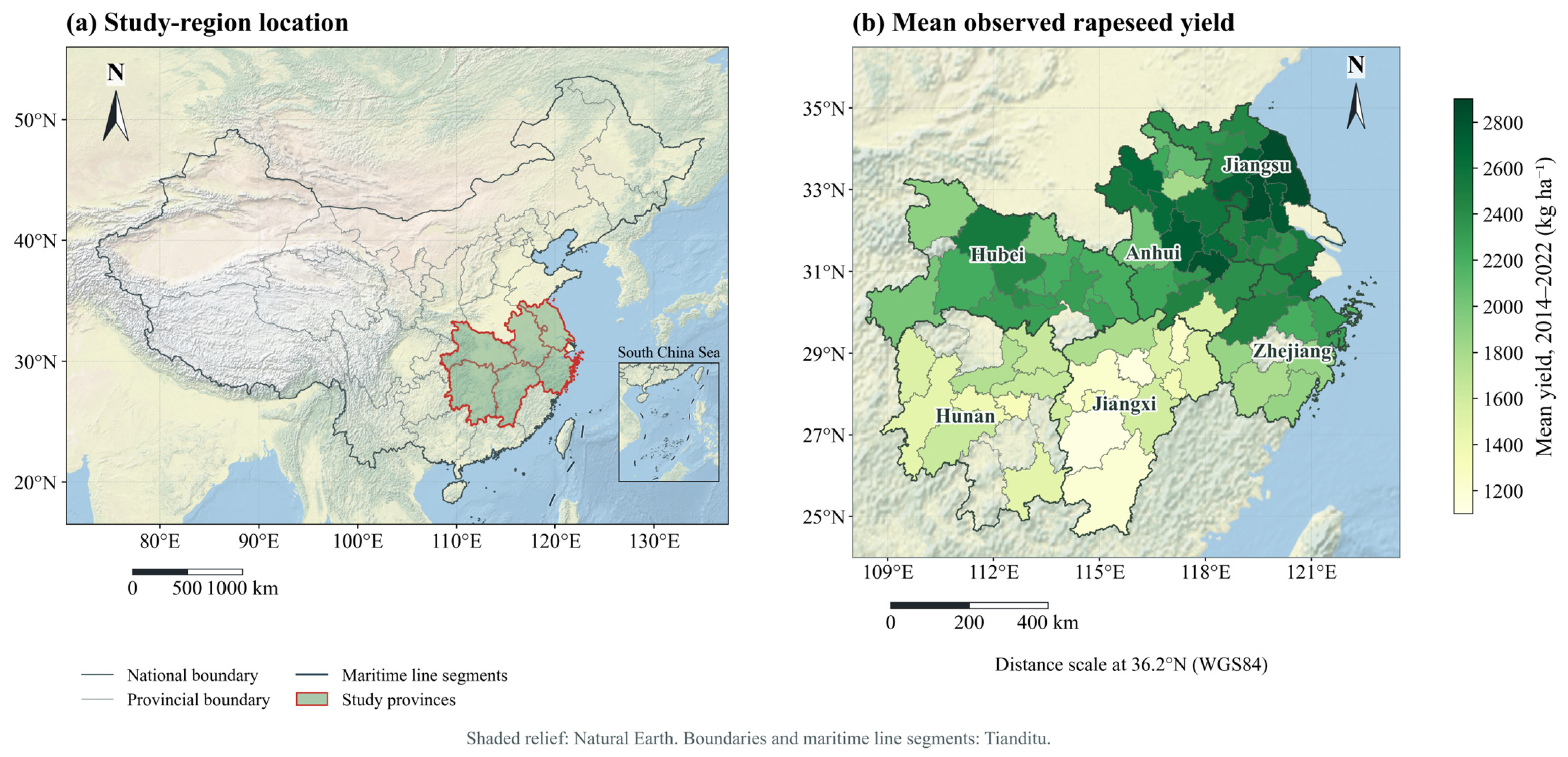
The study area covers 73 prefecture-level cities in the middle and lower reaches of the Yangtze River (MLRYR), spanning Hubei, Hunan, Anhui, Zhejiang, Jiangsu and Jiangxi provinces. In this region, rapeseed is predominantly cultivated in winter rotation with rice (Figure 1) [29]. The MLRYR has a subtropical monsoon climate characterized by warm conditions and abundant precipitation [10]. Rapeseed is sown in autumn (October–November), establishes a rosette and overwinters in the field, bolts and flowers in early spring (February–April), and matures for harvest in May [30]. Consequently, the crop is sequentially exposed to autumn seedling establishment, winter cold, and a wet, variable spring. The overwintering period brings a risk of freeze injury. Flowering and silique filling in spring coincide with the wettest part of the growing season, which increases the risk of waterlogging. In contrast, dry spells that occur between these stages can cause drought stress during stem elongation. Due to this sequence of crop development and the region’s variable weather, the MLRYR provides a relevant setting for evaluating how different climate anomalies affect yield prediction.
The region includes extensive alluvial and lacustrine plains alongside surrounding hills and mountains. For the middle–lower Yangtze plain, FAO describes elevations commonly near 50 m, annual mean temperatures of 14–18 °C and annual precipitation of approximately 1000–1400 mm, concentrated in spring and summer [31].
Figure 1.
Study-area location and city-level mean rapeseed yield. (a) Location of the study provinces in China; the lower-right inset shows the South China Sea as part of the national location reference. (b) Mean city-level rapeseed yield during 2014–2022, compiled from China and provincial statistical yearbooks. Administrative boundaries and maritime line segments were obtained from Tianditu, National Geomatics Center of China [32]. Cities without yield records in the study dataset are left uncolored.
2.2. Data Sources and Feature Construction
This study integrated city-level yield observations, vegetation indices derived from satellite images, TerraClimate meteorological variables, and soil-moisture data. In addition, ERA5-Land data were used specifically for climate-anomaly identification. The data sources, spatial and temporal resolutions, and roles in the framework are summarized in Table 1. Candidate predictor definitions are provided in Table 2.
Table 1.
Data sources, derived variables and their roles in the study.
Table 2.
Definition or formula and source of the twelve candidate predictor variables. NIR, red, and blue are the reflectance of near-infrared, red, and blue bands of Landsat Collection-2 surface-reflectance imagery.
2.2.1. City-Level Yield Observations
City-level winter rapeseed yields for 2014–2022 were compiled from the China Statistical Yearbooks and relevant provincial statistical yearbooks for 73 prefecture-level cities. Of the 657 possible city–year combinations, 115 lacked an available yield record and were excluded without imputation. Matching the available yields with the remotely sensed and meteorological data produced 542 city–year samples. Yield was recorded in t mu−1. For the TCN and BiLSTM, yield was standardized within each cross-validation fold using the mean and standard deviation of the training samples, and predictions were then transformed back to the original unit. The RF and Group Lasso processed the yield data in its unstandardized form. All yields and absolute errors are reported in kg ha−1 (1 t mu−1 = 15,000 kg ha−1).
Annual availability is listed in Table 3. The final monthly predictor matrix contained 45,528 entries (542 records × 84 features), with no missing or infinite entries. Remote-sensing predictors were not interpolated or gap-filled. Across dry, intermediate and wet precipitation thirds within each city, yield-record inclusion was 84.47%, 82.19% and 80.82%, respectively (Table 4).
Table 3.
Availability of yield records by year.
Table 4.
Yield-record inclusion by city-specific precipitation thirds.
2.2.2. Rapeseed Mask and Landsat Vegetation Indices
Rapeseed extent was delineated using the 30 m CARM30 product [33]. Landsat Collection-2 surface-reflectance imagery (30 m) was used to derive NIRv, Normalized Difference Vegetation Index (NDVI) and Enhanced Vegetation Index (EVI). NDVI was used as a general indicator of canopy greenness, while EVI was included to reduce background effects and retain sensitivity under relatively dense vegetation conditions [34]. NIRv was selected because of its closer association with canopy photosynthetic activity and its demonstrated value for rapeseed-yield prediction [22,35]. Observations affected by clouds or shadows were filtered out using the Collection-2 quality assessment band. For each city, the monthly vegetation index was then calculated as the average of the valid pixels within the rapeseed mask.
2.2.3. TerraClimate Meteorological and Soil-Moisture Data
Monthly meteorological and soil-moisture data were obtained from TerraClimate at an approximately 4 km spatial resolution [36]. They comprised precipitation (Pr), maximum temperature (Tmax), minimum temperature (Tmin), soil moisture (SM), solar radiation (Srad), vapor-pressure deficit (VPD), the Palmer Drought Severity Index (PDSI), and potential evapotranspiration (PET). Tmean was calculated as the mean of Tmax and Tmin.
2.2.4. ERA5-Land Data for Climate-Anomaly Identification
ERA5-Land data at the native 0.1° spatial resolution were used only for climate-anomaly identification and were not included as modeling predictors [37]. The two datasets served different purposes: TerraClimate provided monthly predictors for yield modeling, whereas ERA5-Land supplied the finer-temporal-resolution information needed to identify freeze and waterlogging conditions. Daily minimum temperature was used to identify freeze, whereas dekadal precipitation and surface solar radiation were used to derive the waterlogging index (Section 2.3).
2.2.5. City-Level Aggregation and Temporal Feature Construction
For each city and month, NIRv, NDVI and EVI were averaged over valid Landsat pixels within the CARM30 rapeseed mask. Each TerraClimate variable was averaged over all grid cells within the city boundary, without applying the rapeseed mask. Monthly values from November of the sowing year to May of the harvest year were retained as separate features. The predictor set therefore comprised three vegetation indices and nine TerraClimate variables, each represented by seven monthly values, giving 84 features for each city–year sample (12 variables × 7 months). ERA5-Land variables were not included in the predictor set and were used only for climate-anomaly identification.
The vegetation indices describe conditions within mapped rapeseed fields, whereas the TerraClimate averages describe the broader city-scale environmental setting. Both summaries were matched to city-level yield observations.
2.3. Climate-Anomaly Identification and Regime Classification
Three climate-anomaly indicators were constructed using thresholds informed by national and sectoral standards (Table 5). The freeze threshold was informed by the national standard for cold damage to rapeseed, GB/T 27959-2011 [38]. For each ERA5-Land grid cell, the minimum of the daily minimum temperatures was calculated within each month and then averaged over the city. A city–year was classified as freeze-affected when this city-mean monthly minimum fell below −3 °C in any growing-season month (approximately 79% of samples). Drought was identified using PDSI. A city–year sample was classified as drought-affected when its mean growing-season PDSI was below −0.5, the conventional Palmer threshold for incipient drought [39] (approximately 33% of samples).
Table 5.
Identification criteria of climate anomalies.
Waterlogging was assessed using a waterlogging index based on QX/T 107-2009 [40], which was developed for winter wheat and rapeseed. For each dekad, the waterlogging index Qw was calculated using the equation:
where R is dekadal precipitation; Rmax is the maximum dekadal precipitation during the 1991–2020 reference period; DR is the number of precipitation days; D is the number of days in the dekad; S is dekadal sunshine duration; and Smax is the maximum possible sunshine duration for the dekad. R, Rmax, DR and D were derived from ERA5-Land. S was estimated from ERA5-Land surface solar radiation using the FAO-56 Angstrom relation.
For R and DR, daily precipitation was aggregated within each dekad, and the resulting grid-cell values were averaged over the city; a precipitation day was defined as daily precipitation greater than 1 mm. Rmax was calculated as the grid-cell maximum for the corresponding calendar dekad over 1991–2020 and then averaged over the city. Rs was summed within each dekad and spatially averaged before sunshine duration was estimated using the city-centroid latitude.
where Rs is the incoming surface solar radiation, Ra is extraterrestrial radiation, and Smax is the maximum possible sunshine duration defined above. The Angstrom coefficients were set to as = 0.25 and bs = 0.50 [41]. To calibrate the Qw coefficients, principal component analysis (PCA) was applied to 28,080 dekadal records from 2013 to 2022 across the six provinces. The three component indicators (R/Rmax, DR/D and S/Smax) were standardized before PCA. The absolute loading scores weighted by the explained-variance ratios of all three principal components were normalized to sum to one and then linearly mapped to the QX/T 107-2009 coefficient ranges (0.75–1.00 for b1 and b2, and 0.50–0.75 for b3). This procedure yielded b1 = 0.846, b2 = 0.840 and b3 = 0.564. Estimated sunshine duration was bounded between zero and Smax.
S = Smax(Rs/Ra − as)/bs
The dekadal index was then aggregated to five rapeseed phenological stages: pre-winter seedling, overwintering, bolting, flowering and silique filling. For each stage, the maximum of all consecutive two-dekad moving means was compared with the stage-specific thresholds in QX/T 107-2009 (Table 6). As an exception, the bolting stage was evaluated using the maximum single-dekad Qw, in accordance with the standard’s specific requirement for that developmental phase. A stage was classified as waterlogged when any qualifying two-dekad episode, or the single-dekad episode for bolting, reached the relevant severity threshold. A city–year was classified as waterlogging-affected if any stage reached at least the light grade (approximately 50% of samples).
Table 6.
QX/T 107-2009 waterlogging-index (Qw) thresholds by rapeseed stage.
The stage windows follow the calendar adopted from QX/T 107-2009 in Table 6. Bolting and flowering therefore overlap in March, and mid-to-late February is outside the listed windows. Each city–year sample was assigned to one of seven mutually exclusive climate-anomaly regimes: no identified climate anomaly, freeze only, waterlogging only, drought + freeze, freeze + waterlogging, drought + waterlogging, and all three climate anomalies (Table 7). One drought-only city–year was observed but was not treated as a separate regime because n = 1. The seven analyzed regimes therefore comprised 541 of the 542 city–year samples. For the pooled ensemble metrics, the single drought-only sample used the global-weight fallback because a regime-specific R2 could not be estimated from one observation. Thus, it was excluded from regime-specific comparisons.
Table 7.
The seven climate-anomaly regimes: sample counts and mean observed yield (kg·ha−1).
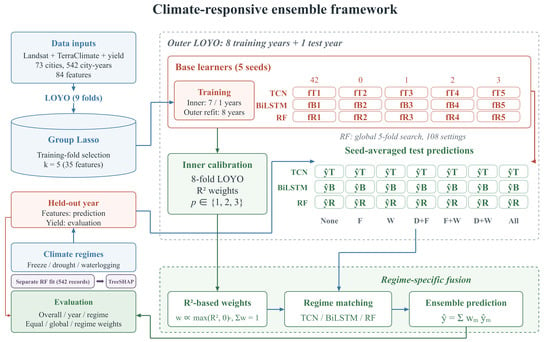
2.4. Climate-Responsive Ensemble Framework Overview
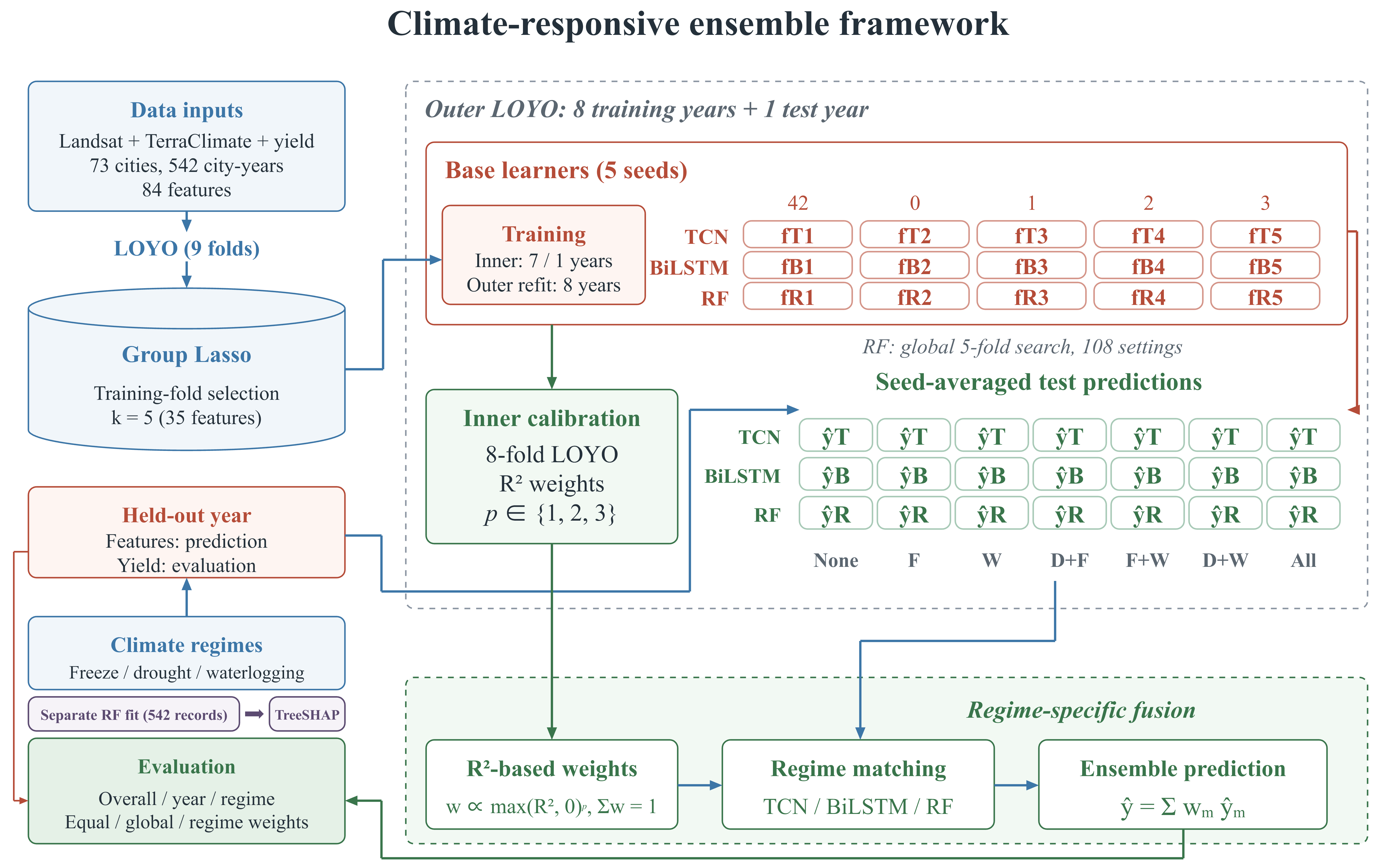
Figure 2 summarizes the five-family main specification with nine outer leave-one-year-out (LOYO) folds. Each outer-training set contains eight years. Eight inner LOYO folds generate validation predictions, with predictor standardization and Group Lasso ranking fitted within each base-fit training partition. Five variable families are retained for each fit. Regime-specific weights and exponent p are calibrated from the inner predictions before the held-out year is predicted.
Figure 2.
Overall workflow of the climate-responsive ensemble framework.
2.5. Group Lasso Feature Selection
The candidate predictor set comprised 12 variables: three Landsat vegetation indices (NIRv, NDVI and EVI) and nine TerraClimate meteorological and soil-moisture variables (Pr, Tmean, Tmax, Tmin, SM, Srad, VPD, PDSI and PET; Table 2). Each variable contributed seven monthly features from November to May, giving 84 candidate features per city–year (12 variables × 7 months). Group Lasso treated the seven monthly features belonging to each variable as one jointly penalized group [42,43]. To prevent data leakage during base-model fitting, standardization and Group Lasso ranking were fitted separately within the training partition of each cross-validation split. The resulting fitted transformations were then applied to the corresponding validation or held-out records. Within each partition, Group Lasso coefficients provided a variable-family ranking from which the top five groups were retained. This procedure was repeated for all outer and inner base-model fits.
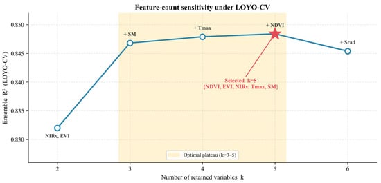
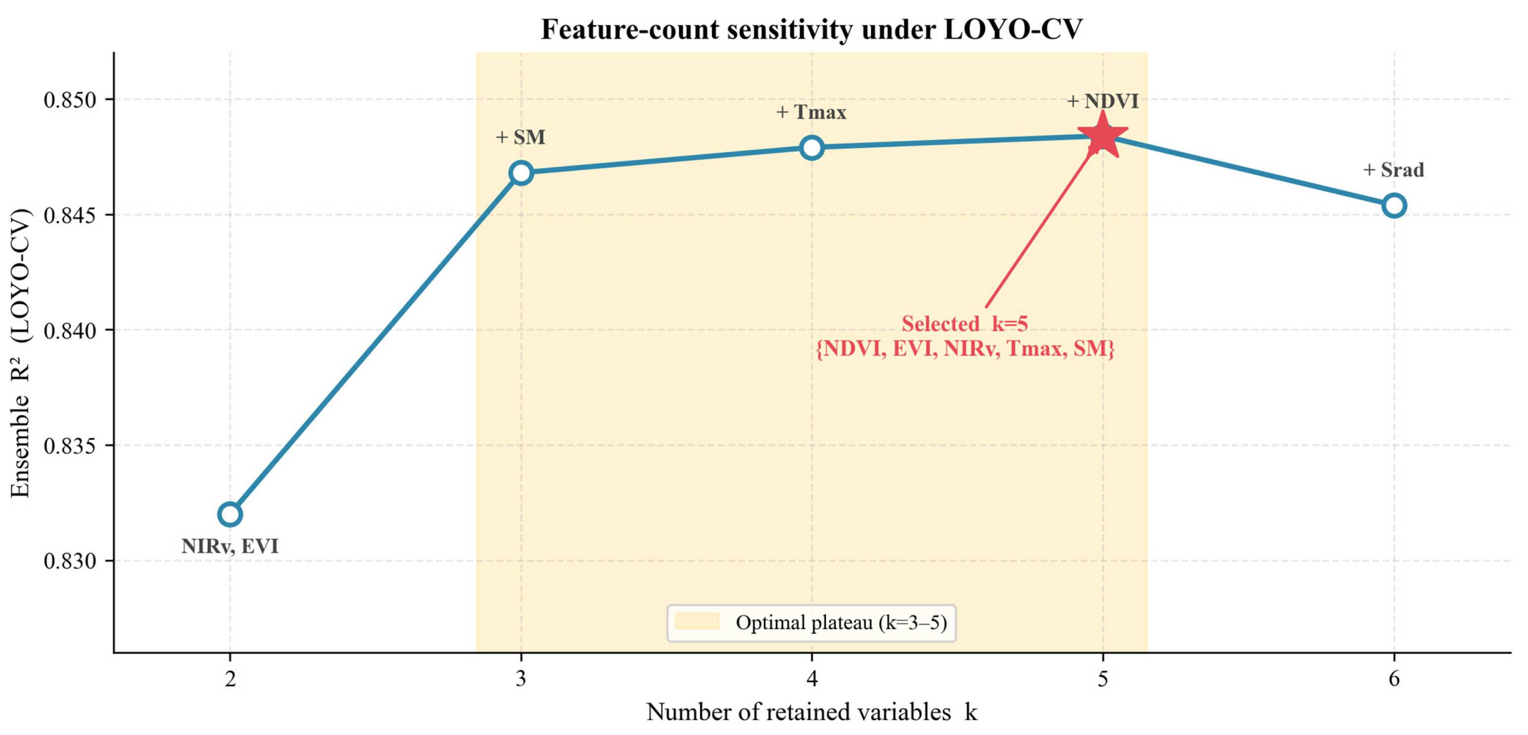
where y is the observed yield vector in t mu−1, X is the standardized design matrix containing the 84 candidate features, β is the complete coefficient vector, and βg is the coefficient vector for variable group g (g = 1,…, 12). Each group contains Pg = 7 monthly features, ||·||2 denotes the L2 norm, and λ is the sparsity penalty selected using the Bayesian information criterion (BIC; [44]). Following the Group Lasso fit, the 12 candidate variables were ranked based on the L2 norm of their respective seven monthly coefficients. The primary model specification retained the top five variable groups. This count was selected during development-stage testing to retain the most informative spectral and meteorological predictors and limit the risk of overfitting in the base learners.
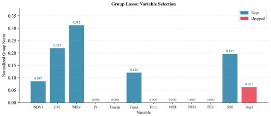
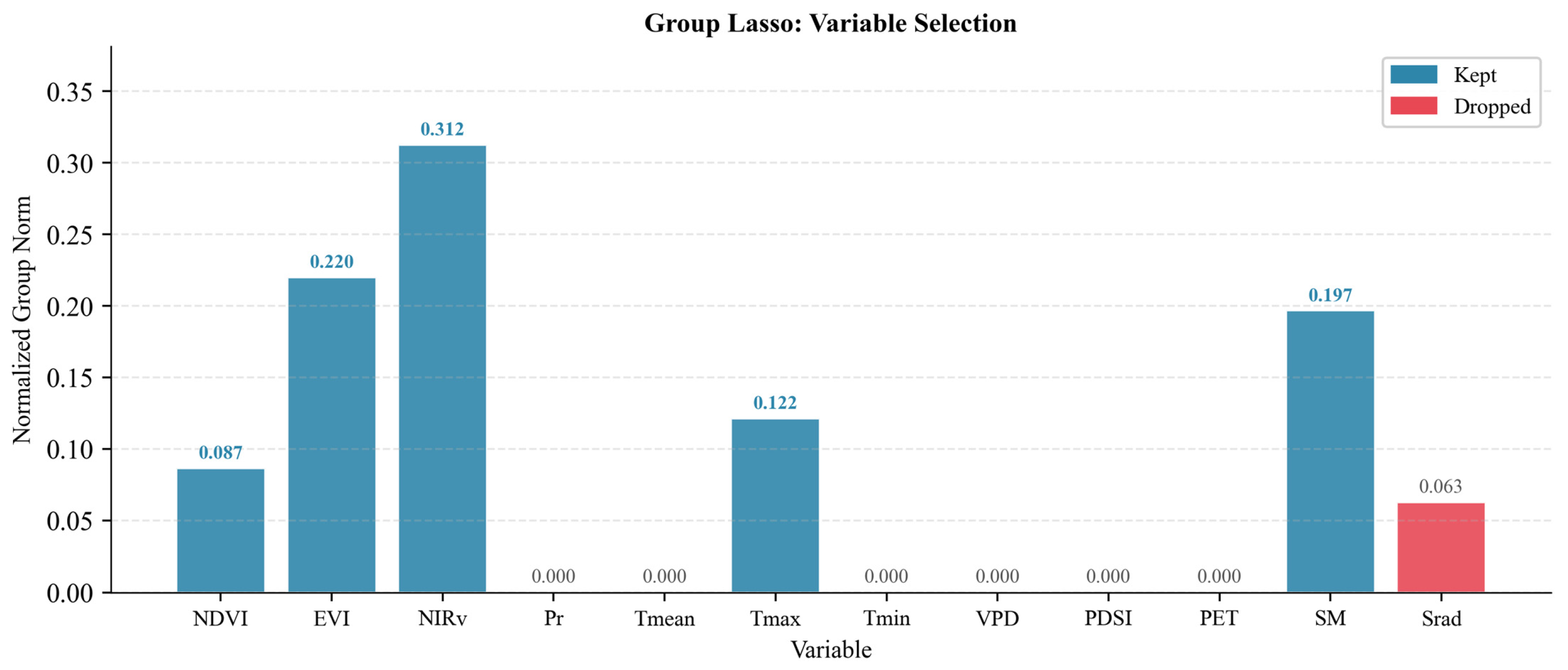
The development analysis ranked NIRv, EVI, SM, Tmax and NDVI as the five leading variable groups (Figure 3), with the supporting feature-count evaluation detailed in Figure 4.
Figure 3.
Group Lasso group norms of the twelve candidate variables in the development analysis.
Figure 4.
Development-stage sensitivity of pooled LOYO-CV R2 to the number of retained variable groups (k = 2–6).
2.6. Base Models and Climate-Responsive Ensemble Model Construction
TCN, BiLSTM and RF were selected because they offer three complementary ways of learning from the same temporal predictors. The TCN captures local and multi-scale temporal patterns through dilated causal convolutions. The BiLSTM represents bidirectional dependencies across the growing-season sequence, while the RF provides a non-sequential benchmark that captures nonlinear and threshold-like relationships. These diverse model structures allow relative performance to vary across climate-anomaly regimes. After Group Lasso selection, each city–year sample was represented by five temporal variables observed over seven months, yielding a 7 × 5 temporal input matrix. The TCN and BiLSTM processed this matrix as a monthly sequence, whereas the RF received the corresponding 35-element flattened feature vector.
The TCN consisted of three residual blocks, each with two dilated causal convolutional layers, with kernel size 3 and block dilations of 1, 2 and 4. This provides a theoretical receptive field of 29 time steps, more than sufficient for the seven-month input sequence while retaining the temporal structure [45,46,47]. The BiLSTM used two stacked layers with a hidden size of 64 to capture bidirectional seasonal dependencies [48,49]. Both TCN and BiLSTM were trained with AdamW under mean-squared-error loss, with dropout and early stopping applied within the outer-training data [50,51]. The RF used a regression-tree ensemble to learn nonlinear and threshold-like interactions from the flattened predictors [52]. Each base learner was trained with five random seeds, and their predictions on held-out data were averaged before ensemble weighting. Network architectures and training hyperparameters were held constant across folds. Seed averaging was used to reduce variability in optimization [53]. Model architectures and hyperparameters are listed in Table 8.
Table 8.
Architectures and key hyperparameters.
RF hyperparameters were selected once by a global search. Following standardization and Group Lasso selection on all 542 records, an ordinary five-fold GridSearchCV procedure compared 108 configurations using mean validation R2: 300, 500, or 800 trees; maximum depth of None, 10, or 20; minimum leaf size of 2, 3, 4 or 5; and max_features of sqrt, 0.5, or 0.6. The folds followed the input row order without shuffling. The selected configuration was shared by all outer and inner training partitions and all five seeds. Each prediction forest was fitted to its corresponding training records.
The ensemble was designed to use the strengths of each base learner across different climate-anomaly regimes. We compared three ensemble strategies: equal weighting, global weighting, and regime-specific weighting, which assigns a separate set of weights for each climate-anomaly regime. Equal weighting assigns one-third of the total weight to each learner, irrespective of its estimated skill, while global weighting uses a single set of weights reflecting overall performance. In contrast, regime-specific weighting lets the ensemble assign more weight to the model that performs best for each type of climate anomaly. The other models can still contribute when their regime-specific R2 values are positive. For each city–year sample i, the climate-anomaly regime g was assigned using the criteria in Section 2.3. The final ensemble prediction was the convex combination of the three base-model predictions (Equations (4) and (5)).
where ŷi is the ensemble prediction for sample i, ŷm, i is the prediction from base model m, and wm,g is the weight assigned to model m for the climate-anomaly regime g of sample i (m, m′ ∈ {TCN, BiLSTM, RF}). denotes the model-specific R2 within regime g, and p is the sharpening exponent. Negative R2 values were truncated to zero before normalization. Regimes with fewer than 10 inner records, an absent group or an undefined R2 used the training-only global weights. If the global non-negative scores summed to zero, equal weights were used.
Within each outer fold, each record in its eight training years received one five-seed-averaged inner validation prediction from each base learner. Regime-specific R2 values used only these inner predictions and their corresponding yields. Global weights used all inner validation records within the same outer-training set. Candidate exponents p = 1, 2 and 3 were compared by pooled inner-validation ensemble R2, retaining k = 5. Weights and the selected exponent were fixed before predicting the held-out year. The global-weight comparator selected its exponent from the same candidate set using its own inner-validation R2. The equal-weight comparator averaged the TCN, BiLSTM, and RF predictions, giving each model a weight of 1/3. Inner validation selected p = 3 in all nine outer folds for both the regime-specific and global weighting strategies.
2.7. Experiment Design and Performance Evaluation
The main analysis used nine outer LOYO folds, each with eight training years and one held-out year. Within an outer-training set, each of the eight inner LOYO folds used seven years for training and the remaining year for validation. Predictor standardization, Group Lasso ranking, and base-learner fitting were carried out within each inner-training partition. Early stopping for the neural networks used a seeded validation subset from those training years. The five-family count and neural-network configurations remain fixed, while variable identities followed the partition-specific GL ranking. RF hyperparameters were the common configuration selected by the global search described in Section 2.6. After inner weight and exponent calibration, scaling, GL ranking and base learners were fitted on the eight outer-training years to predict the held-out year. The predictions from all nine held-out years were pooled for evaluation.
Predictive performance was compared among the three base learners, the equal-weight ensemble, the global-weight ensemble and the climate-responsive weighted ensemble. Predictions were transformed back to the original yield scale before the R2 (Equation (6)), RMSE (Equation (7)), MAE (Equation (8)) and rRMSE (Equation (9)) were calculated.
where yi and ŷi are the observed and predicted yield of sample i, ȳ is the mean observed yield, and n is the number of samples; rRMSE is expressed as a percentage of the regional mean yield.
Table 9 report paired record-level bootstrap intervals from 2000 resamples. Complete city–year records were sampled independently with replacement, with the same sampled records applied to all prediction strategies. Pooled uncertainty analysis used 50,000 paired two-way pigeonhole bootstrap resamples over the 73 cities and nine years [54]. Cities and years were sampled independently with replacement, and each observed city–year received the product of its city and year multiplicities. These identical multiplicities were maintained across all modeling strategies, and two-sided 95% percentile intervals were constructed from the pooled RMSE differences.
Table 9.
Comparisons of RMSE among ensemble weighting strategies at p = 3.
Additionally, a sensitivity analysis was conducted using the delta-method influence function for each paired RMSE contrast. This utilized the CGM (city-plus-year-minus-intersection) covariance estimator, incorporating finite-cluster corrections and t-distribution critical values with eight degrees of freedom [55]. All predictions, feature choices, hyperparameters and ensemble weights were held fixed. The regime-level comparisons in Table 9 were exploratory. RMSE contrasts were calculated as follows:
where EA, GW and RS denote the equal-average, global-weight and regime-specific weighting strategies, respectively; ENS denotes the ensemble; and m denotes a base learner (TCN, BiLSTM or RF). The first two contrasts are reported in Table 9. Positive values indicate a lower RMSE for the regime-specific weighting strategy in Equations (10) and (11), or for the ensemble in Equation(12). For both bootstrap analyses, the lower and upper bounds of the 95% intervals were taken as the 2.5th and 97.5th percentiles of the bootstrap distribution [56]. All analyses and model implementations were conducted in Python 3.9.18 (Python Software Foundation, Beaverton, OR, USA), using PyTorch 2.5.1, scikit-learn 1.3.2, group-lasso 1.5.0, SHAP 0.48.0, NumPy 1.26.4, pandas 2.3.3, and SciPy 1.12.0. Python-based plotting was performed using Matplotlib 3.9.2.
ΔRMSEEA−RS = RMSEEA − RMSERS
ΔRMSEGW−RS = RMSEGW − RMSERS
ΔRMSEm−ENS = RMSEm − RMSEENS
2.8. Model Interpretation Using SHAP
A separate RF model was used for interpretation because TreeSHAP provides exact and computationally efficient explanations for tree-based models. This interpretation model was fitted to all 542 records using the five selected variables, with 500 trees, max_features = sqrt, min_samples_leaf = 3, and a fixed random seed of 42. TreeExplainer was used because it provides exact and computationally efficient Shapley-value estimates for tree ensembles [57,58]. For each city–year sample, the sign of a SHAP value indicates whether a feature increases or decreases the RF-predicted yield relative to the model’s baseline prediction, and its absolute value indicates the strength of its contribution. Global feature importance was calculated as the mean absolute SHAP value across all samples. Regime-specific importance was calculated separately within each regime, and monthly summaries were obtained by aggregating absolute SHAP values by month and variable.
RF SHAP values are expressed in kg ha−1 by multiplying the original t mu−1 values by 15,000. The held-out stability check used 45 saved RF models, five seeds for each of nine outer folds, with the shared five-variable selection and globally chosen RF configuration (800 trees, depth 10, max_features = sqrt and minimum leaf size 2). Their predictions were matched to the corresponding held-out RF predictions before attribution. Signed SHAP values and expected values were averaged over seeds, and local additivity was checked against the seed-averaged predictions. Fold-specific feature rankings were compared with the interpretation-model ranking and with other folds.
3. Results
3.1. Regime-Dependent Model Skill and Weighting Strategy
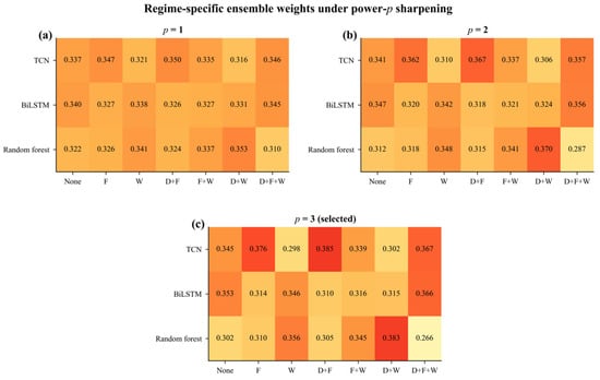
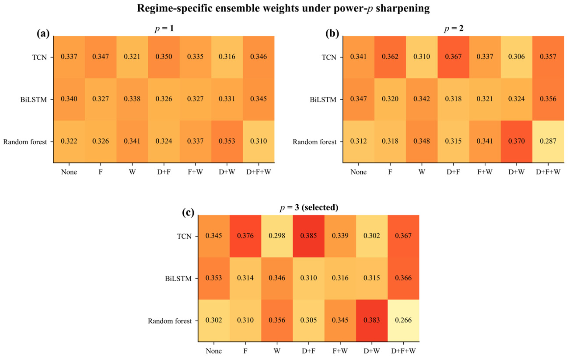
To determine whether model suitability changed across climate-anomaly regimes, we first examined the regime-specific performance of the three base learners and the resulting ensemble weights. The sharpening exponent p determined how heavily the ensemble favoured the best-performing model in each regime. As p increased from one to three, the weighting became more concentrated on the strongest performer, while retaining non-zero contributions from learners with positive R2. The regime-specific ensemble weights for p = 1–3 are shown in Figure 5.
Figure 5.
Regime-specific ensemble weights for (a) p = 1, (b) p = 2, and (c) p = 3. None denotes no identified climate anomaly; F, D and W denote freeze, drought and waterlogging, respectively. Each cell shows the mean weight across nine outer folds, with fold-specific weights estimated from inner validation predictions.
At p = 3, RF received the highest mean weights under waterlogging only (0.356), freeze + waterlogging (0.345), and drought + waterlogging (0.383). TCN received the highest mean weights under freeze only (0.376) and drought + freeze (0.385). TCN and BiLSTM had nearly equal mean weights when all three climate anomalies co-occurred (0.367 and 0.366, respectively; Figure 5c).
At p = 3, the equal-average, global-weight and regime-specific ensembles yielded overall RMSE values of 190.1, 189.8 and 189.0 kg·ha−1, respectively (Table 9). In the pooled dependence-aware analysis, regime-specific weighting reduced the RMSE by 1.09 kg·ha−1 relative to equal averaging (95% CI [0.14, 2.18]) and by 0.85 kg·ha−1 relative to global weighting (95% CI [0.10, 1.71]). Across regimes, the largest improvements relative to global weighting occurred under drought + waterlogging (2.48 kg·ha−1) and the co-occurrence of all three climate anomalies (2.09 kg·ha−1), while the largest improvements relative to equal averaging also appeared when all three climate anomalies co-occurred (2.72 kg·ha−1).
3.2. Predictive Performance of the Base Learners and Ensemble
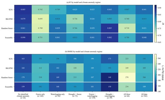
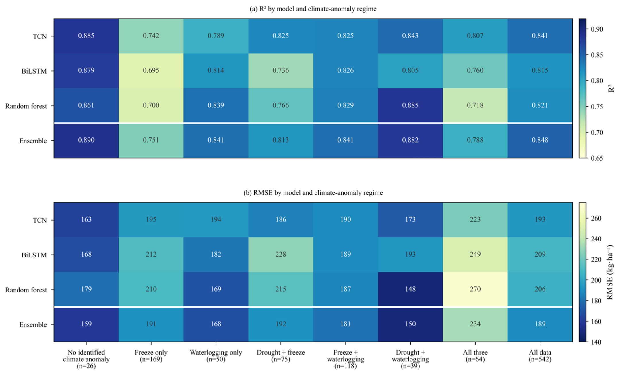
The performance of three base models varied across climate-anomaly regimes (Figure 6). The TCN achieved the highest R2 under no identified climate anomaly, freeze only, drought + freeze, and the co-occurrence of all three climate anomalies, whereas the RF yielded the most accurate predictions under waterlogging only, freeze + waterlogging, and drought + waterlogging.
Figure 6.
Model performance across climate-anomaly regimes: (a) R2 and (b) RMSE (kg·ha−1). The final column reports performance across all 542 samples.
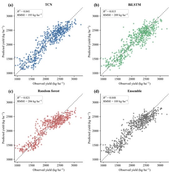
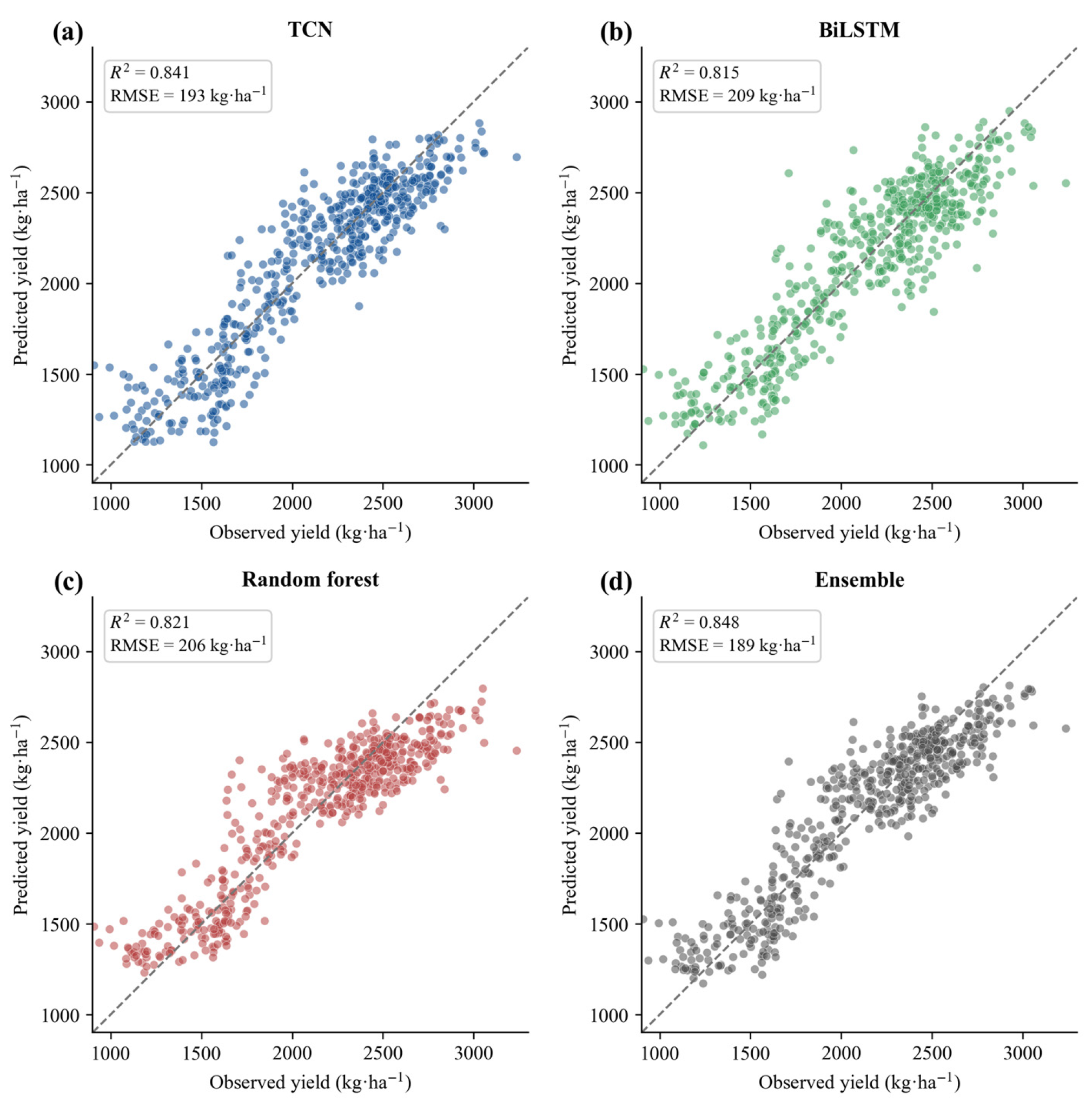
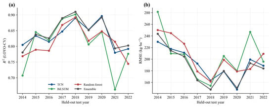
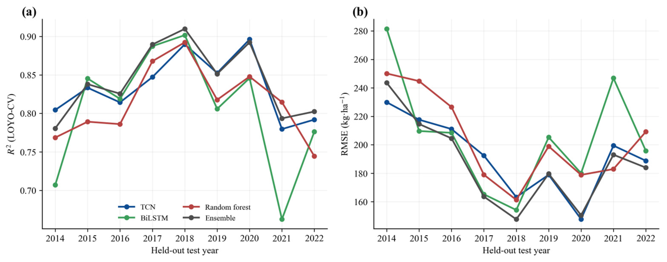
Given these regime-dependent differences among the base learners, we further evaluated the overall predictive performance of the final regime-specific ensemble relative to the three individual models. Across all 542 city–year samples, the ensemble achieved R2 = 0.848, RMSE = 189 kg·ha−1, MAE = 151 kg·ha−1 and rRMSE = 8.9%, and had the most favorable descriptive metrics among the four models (Table 10). The TCN was the strongest base learner (R2 = 0.841; RMSE = 193 kg·ha−1), followed by the RF (R2 = 0.821; RMSE = 206 kg·ha−1) and BiLSTM (R2 = 0.815; RMSE = 209 kg·ha−1). Observed and predicted yields for all four models followed the 1:1 relationship (Figure 7). In the year-wise summary of the calibrated ensemble, R2 ranged from 0.781 in 2014 to 0.910 in 2018, and RMSE ranged from 148 to 244 kg·ha−1 (Figure 8).
Figure 7.
Observed versus predicted yield (kg·ha−1) under LOYO-CV for (a) the TCN, (b) the BiLSTM, (c) the random forest and (d) the climate-responsive ensemble; the dashed line is the 1:1 reference.
Figure 8.
Year-by-year accuracy across the nine LOYO folds: (a) R2 and (b) RMSE for each held-out year.
Table 10.
Overall performance of the base learners and calibrated ensemble (n = 542).
Regime-specific weighting reduced annual RMSE relative to equal and global weighting in seven and eight of the nine years, respectively (Table 11).
Table 11.
Annual RMSE and weighting-strategy gains (kg ha−1).
3.3. Evaluation Under Climate-Anomaly Regimes and Spatial Patterns
Aggregate accuracy may conceal model differences within individual climate-anomaly regimes. We therefore compared the ensemble with individual models within climate-anomaly regimes (Table 12), assessed cross-regime robustness, and examined whether its predicted spatial patterns agreed with observed yield patterns.
Table 12.
Within-regime RMSE differences between each base learner and the regime-specific ensemble, with paired record-level bootstrap 95% intervals (B = 2000).
Predictive accuracy varied substantially across climate-anomaly regimes. The ensemble achieved its highest R2 under no identified climate anomaly and drought + waterlogging, intermediate values under waterlogging only and freeze + waterlogging, and its lowest value under freeze only (Figure 6). RMSE ranged from 150 kg·ha−1 under drought + waterlogging to 234 kg·ha−1 when all three climate anomalies co-occurred. Compared with the TCN, the ensemble reduced RMSE by 25.57 kg·ha−1 under waterlogging only, by 8.98 kg·ha−1 under freeze + waterlogging and by 22.67 kg·ha−1 under drought + waterlogging (Table 12).
Across all 542 city–year records, the pooled RMSE reductions relative to TCN, BiLSTM and RF were 4.53, 19.74 and 16.61 kg·ha−1, respectively. Table 13 reports the corresponding city-by-year intervals together with the two weighting-strategy comparisons.
Table 13.
Pooled RMSE differences with paired city-by-year bootstrap 95% intervals.
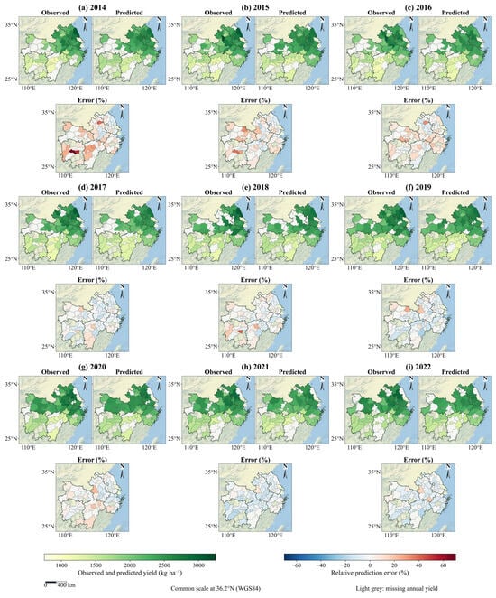
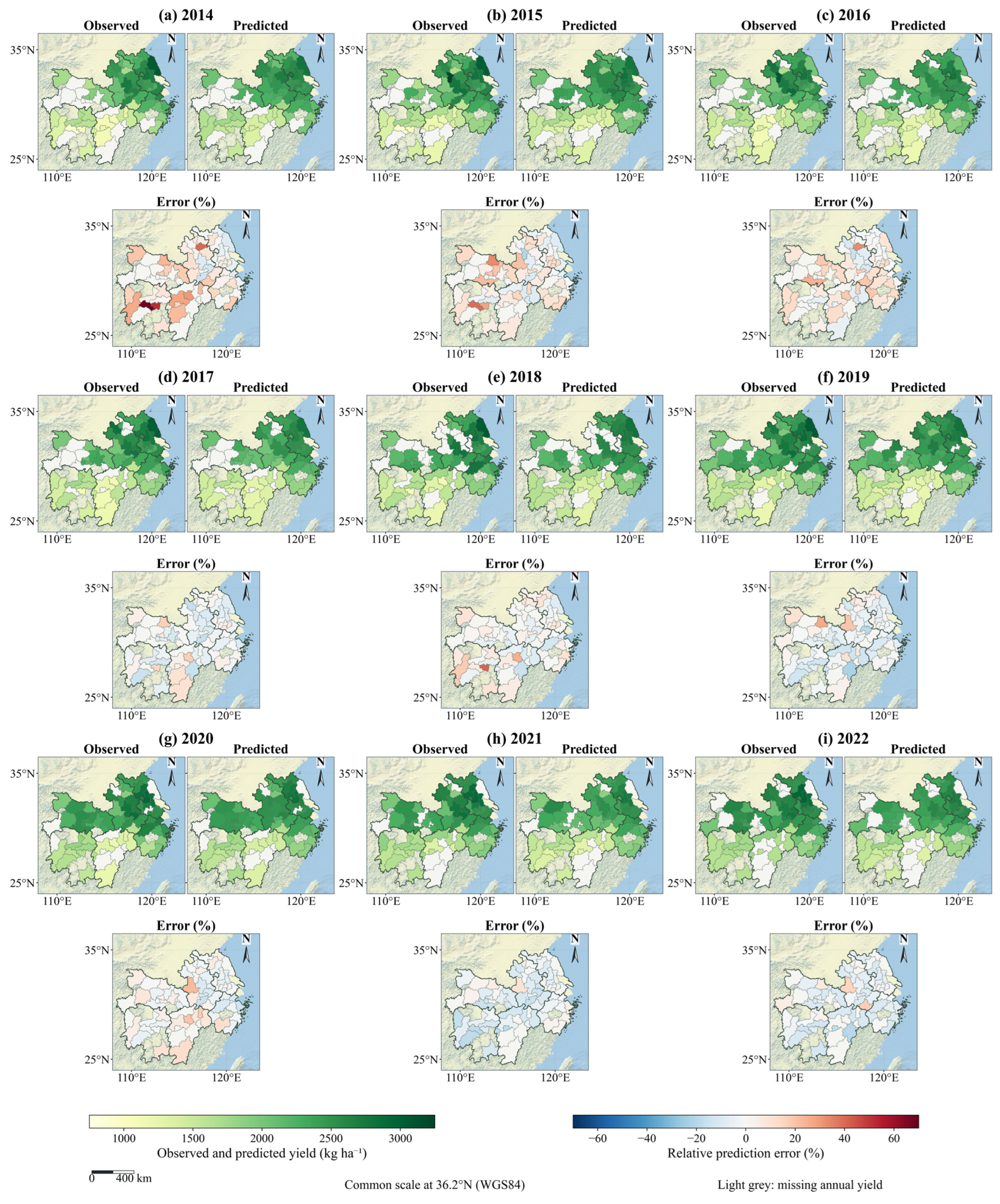
Observed yield, ensemble predictions and relative prediction error were mapped for all nine held-out years (Figure 9). The maps reproduced broad annual spatial contrasts, with residuals varying among years.
Figure 9.
Annual spatial distributions of observed yield, ensemble-predicted yield and relative prediction error (%) for the nine held-out years (2014–2022). Panels (a–i) correspond to individual years; within each panel, observed yield, predicted yield and relative error are shown with common color scales. Areas without an available annual yield record are left uncolored.
3.4. Model Interpretation
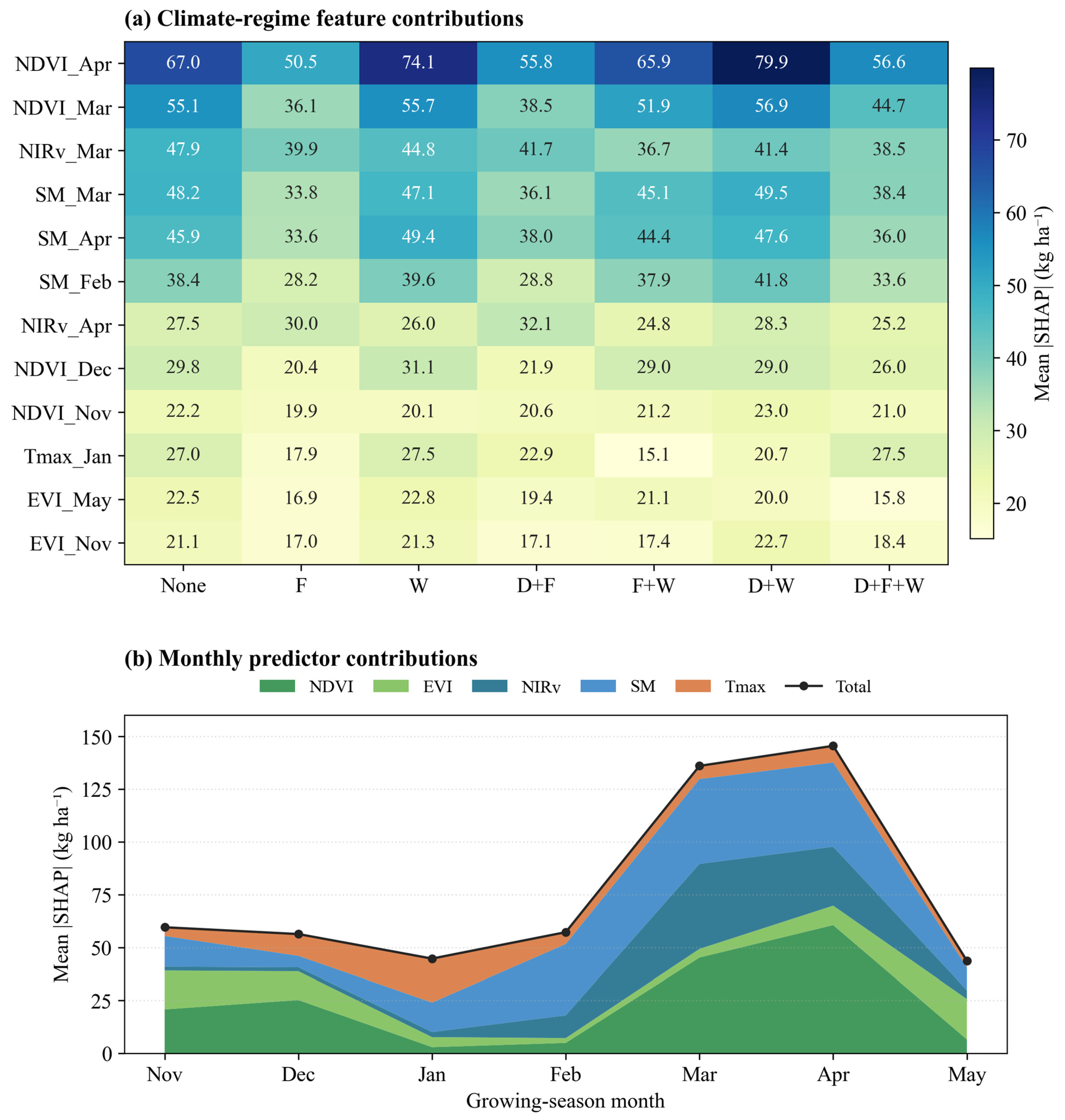
SHAP analysis of the RF highlighted March–April vegetation indices and February–April soil moisture as the most influential predictors, with temperature features contributing less overall (Figure 10a). At the variable level, NDVI, NIRv and EVI together accounted for approximately 60% of the total mean absolute SHAP importance, soil moisture for roughly 29%, and Tmax for about 11%. The beeswarm plot showed that higher spring vegetation index values were generally associated with positive SHAP values and higher RF-predicted yields, whereas higher spring soil moisture was generally associated with negative SHAP values and lower RF-predicted yields (Figure 10b). Across climate-anomaly regimes, April NDVI remained the most influential feature, especially under drought + waterlogging and waterlogging only. Soil-moisture features from February to April were also more important in these waterlogging-affected regimes than under freeze only (Figure 11a).
Monthly mean absolute SHAP values were relatively low from November to February, peaked in March and April, and declined in May (Figure 11b). Vegetation indices and soil moisture were the main contributors to the high total SHAP importance observed in March and April, whereas the relative contribution of Tmax was greater during the winter months.
Held-out RF attribution reproduced the main interpretation-model pattern (Table 14). The correlation between the 35-feature mean absolute SHAP rankings was Spearman ρ = 0.992; fold-specific correlations with the interpretation-model ranking ranged from 0.941 to 0.982. NDVI, EVI and NIRv together contributed 59.81% of held-out mean absolute SHAP importance, SM 28.49% and Tmax 11.70%. Local SHAP sums reproduced the five-seed mean RF predictions with maximum error below 3 × 10⁻¹² kg ha−1.
Table 14.
Variable-level mean absolute SHAP shares in the interpretation and held-out RF models (%).
Figure 10.
SHAP values for the separate RF model. (a) Global mean absolute SHAP values for feature importance. (b) Beeswarm plot showing the direction and distribution of feature contributions to RF predictions. All SHAP contributions are expressed in kg ha−1.
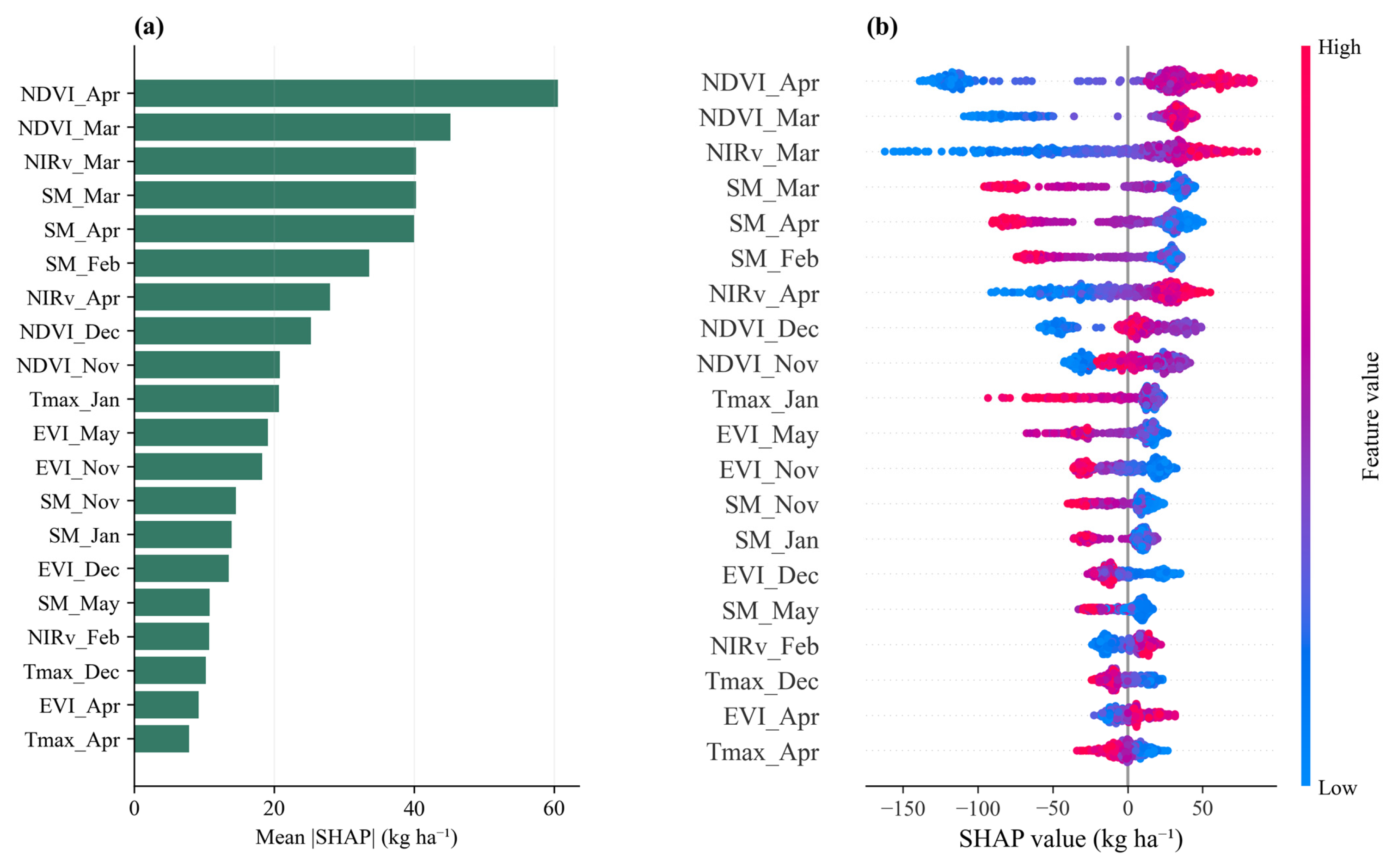
Figure 11.
SHAP values for the separate RF model (contributions in kg ha−1). (a) Mean absolute SHAP values for the top 12 features across seven climate-anomaly regimes. (b) Monthly mean absolute SHAP importance for each predictor variable, aggregated from November to May.
3.5. Sensitivity to Climate-Anomaly Definitions
Sample counts and predictive performance under alternative drought, freeze and waterlogging criteria are summarized in Table 15. The pooled ensemble RMSE was 188.96 kg ha−1 under the original criteria and ranged from 188.39 to 189.07 kg ha−1 under the alternatives. Even when the criteria changed regime labels, the pooled RMSE differed from the original value by at most 0.57 kg ha−1 (0.30%).
Table 15.
Sensitivity to climate-anomaly definitions. Δn counts records with a changed regime label. RMSE and gains are in kg ha−1.
4. Discussion
4.1. Climate-Anomaly-Dependent Model Performance
Model performance varied across the evaluated climate-anomaly regimes. The TCN was the strongest base learner overall and led under four regimes, whereas the RF led under the three waterlogging-related regimes. Against this background, the climate-responsive ensemble achieved R2 = 0.848, RMSE = 189 kg·ha−1 and rRMSE = 8.9% in the pooled analysis of nine years and 73 cities.
Although there are few regional deep learning studies on winter rapeseed, comparisons with studies on other crops provide useful context. For example, winter wheat models have reported R2 values of 0.64–0.81 and RMSE between 462 and 617 kg·ha−1 under similar validation schemes [59,60], while a county-level soybean CNN–LSTM reported an average end-of-season RMSE of 329.53 kg·ha−1 with annual R2 values of 0.69–0.81 [61]. These comparisons are not direct benchmarks, as crop type, spatial scale, and yield range differ among studies, and they cannot establish relative predictive superiority. This study introduces a distinct capability by conditioning model fusion on explicit climate-anomaly regimes, extending previous approaches that used only global weighted combinations [62].
These regime-dependent rankings show how the relative performance of the individual learners varies with climate-anomaly conditions. The ensemble adjusts model contributions by regime. Compared with the TCN, its RMSE was lower by 25.57 kg·ha−1 under waterlogging only and by 8.98 kg·ha−1 under freeze plus waterlogging (Table 12). The regime-specific weights provide an explicit record of model-level contributions.
The pooled dependence-aware analysis provides a common comparison across weighting strategies and individual learners (Table 13). RMSE gains relative to equal and global weighting were 1.09 kg·ha−1 (95% CI [0.14, 2.18]) and 0.85 kg·ha−1 (95% CI [0.10, 1.71]), respectively. The corresponding CGM sensitivity intervals were [0.23, 1.96] and [0.15, 1.56] kg·ha−1. Relative to the three individual learners, pooled RMSE gains ranged from 4.53 to 19.74 kg·ha−1.
For end-of-season monitoring, the framework can generate yield estimates once the required Landsat, TerraClimate, and ERA5-Land inputs through May are available.
4.2. Regime-Specific Model Interpretation
SHAP analysis characterized how the selected predictors contributed to the RF yield estimates. Spring vegetation indices emerged as the dominant predictors, capturing critical canopy development during the flowering and silique-filling stages. Since NDVI, EVI, and NIRv provide correlated information regarding canopy condition and photosynthetic activity [35], SHAP can distribute shared predictive information among them. Their combined vegetation contribution is therefore more informative than treating a single-index ranking as an independent physiological effect.
Spring soil moisture also showed a strong, predominantly negative contribution to rapeseed yield predictions. This is consistent with agronomic evidence that waterlogging and root-zone hypoxia during flowering and seed filling can impair root function and reduce rapeseed yield and yield components [12,13]. Higher January temperature was also associated with lower yield predictions, which may reflect the role of winter temperature in the vernalization and flowering development of winter rapeseed [63]. These attribution patterns support the model’s biological plausibility, though they represent associative rather than strict causal relationships.
Seasonal attribution showed that the total mean absolute SHAP importance peaked in March and April, driven mainly by vegetation indices and soil moisture, whereas the relative contribution of Tmax was greater during winter. The spring peak coincided with flowering and early silique development, when canopy condition and root-zone water status are closely related to reproductive growth and seed set [12,13]. The greater winter contribution of Tmax is consistent with the role of temperature in vernalization and overwintering development, while freeze stress can affect subsequent yield formation [11,63]. Temperature is also important during reproductive development: high-temperature stress during flowering can reduce reproductive fertility, fruit and seed development, and seed weight in Brassica napus [64]. These stage-specific effects help explain the seasonal differences in temperature attribution. Taken together, the results indicate that meteorological context was associated with stage-specific changes in model attribution.
4.3. Limitations and Future Work
With nine observed years, the resampling intervals summarize uncertainty for this study period. Evaluation across additional years and regions would extend the evidence for temporal and geographic transfer.
Second, the current meteorological indicators have inherent constraints. The freeze indicator relies on city-averaged monthly minimum temperatures, which cannot resolve the exact duration or accumulated intensity of acute cold events. Growing-season mean PDSI can mask short drought episodes during sensitive stages. Although the threshold and seasonal-window checks in Table 15 changed regime membership substantially, the pooled ensemble RMSE remained stable (188.39–189.07 kg ha−1). These fixed-prediction checks assess grouping and weight-calibration sensitivity.
The analysis used prefecture-level yields for 542 city–year samples, with predictors drawn from both high-resolution (Landsat, 30 m) and lower-resolution (TerraClimate, ~4 km) sources. Vegetation indices were restricted to rapeseed pixels, whereas climate variables were averaged over the full city. Using the 2020 harvest season as a sample, rapeseed-area-weighted and city-wide climate averages were compared across 73 cities and seven months. The mean absolute differences were 0.334 °C for Tmax and 2.89 mm for SM, indicating small average input differences between the two aggregation approaches. Future research may move toward pixel-level yield modeling, allowing climate-responsive models to capture localized microclimate responses. Because temporal holdout does not test geographic transfer, spatially structured validation should also be considered before applying the model to new areas [65].
This study did not evaluate external transferability, so applying the model outside the MLRYR will require separate validation. Domain-adaptation techniques or updating regime weights may facilitate transfer to new areas [66], and re-estimating only the regime weights may offer a lower-cost alternative.
5. Conclusions
This study proposes a climate-responsive weighted ensemble for regional winter rapeseed yield prediction, designed to overcome the limitations of static models under varying meteorological stresses. Evaluated across 73 prefecture-level cities in the middle and lower reaches of the Yangtze River, the ensemble achieved high overall accuracy (R2 = 0.848, RMSE = 189 kg·ha−1, and rRMSE = 8.9%). By dynamically adjusting the fusion weights of three base models according to explicit climatic regimes, the ensemble reduced the prediction errors compared to the TCN, particularly under isolated waterlogging and compound freeze-waterlogging events.
Rigorous climate-anomaly-dependent analysis confirmed the statistical value of the proposed approach, yielding pooled RMSE reductions of 1.09 and 0.85 kg·ha−1 relative to equal and global weighting, respectively. Furthermore, SHAP analysis validated the framework’s agronomic plausibility by identifying spring vegetation indices and soil moisture as dominant predictors, correctly capturing intensified soil-moisture sensitivity under waterlogging and drought–waterlogging regimes. Future work should refine this approach by: (1) integrating continuous thermal metrics to capture cold-stress intensity and duration; (2) transitioning to higher-resolution data for localized modeling; and (3) testing the spatial transferability to other major rapeseed-producing regions using domain-adaptation strategies.
Author Contributions
S.D.: Conceptualization, Methodology, Software, Formal analysis, Investigation, Data curation, Validation, Visualization, Writing—original draft, Writing—review and editing. H.M.: Methodology, Software, Formal analysis, Validation, Writing—review and editing. T.L.: Data curation, Investigation, Validation, Visualization. P.L.: Data curation, Resources, Validation. D.H.: Resources, Validation. Q.G.: Supervision. S.L.: Conceptualization, Methodology, Supervision, Project administration, Funding acquisition, Writing—review and editing. All authors have read and agreed to the published version of the manuscript.
Funding
This work was supported by the earmarked fund for China Agriculture Research System [grant number CARS-12]. The funder had no role in study design, data collection, data analysis or interpretation, manuscript preparation, or the decision to submit the article for publication.
Data Availability Statement
The data and code supporting this study are openly available in Zenodo at https://doi.org/10.5281/zenodo.24096224.
Conflicts of Interest
Shishi Liu serves as a Guest Editor of this Special Issue. The authors declare no other conflicts of interest.
References
- Bonjean, A.P.; Dequidt, C.; Sang, T. Rapeseed in China. OCL—Oilseeds Fats Crops Lipids 2016, 23, D605. [Google Scholar] [CrossRef] [Scilit]
- Tian, Z.; Ji, Y.; Xu, H.; Qiu, H.; Sun, L.; Zhong, H.; Liu, J. The potential contribution of growing rapeseed in winter fallow fields across the Yangtze River Basin to energy and food security in China. Resour. Conserv. Recycl. 2021, 164, 105159. [Google Scholar] [CrossRef] [Scilit]
- Fang, Y.T.; Ren, T.; Zhang, S.T.; Liu, Y.; Liao, S.P.; Li, X.K.; Cong, R.H.; Lu, J.W. Rotation with oilseed rape as the winter crop enhances rice yield and improves soil indigenous nutrient supply. Soil Tillage Res. 2021, 212, 105065. [Google Scholar] [CrossRef] [Scilit]
- Han, X.; Chen, Q.; Fu, D. Trends in extreme precipitation and associated natural disasters in China, 1961–2021. Climate 2025, 13, 74. [Google Scholar] [CrossRef] [Scilit]
- Vogel, E.; Donat, M.G.; Alexander, L.V.; Meinshausen, M.; Ray, D.K.; Karoly, D.; Meinshausen, N.; Frieler, K. The effects of climate extremes on global agricultural yields. Environ. Res. Lett. 2019, 14, 054010. [Google Scholar] [CrossRef] [Scilit]
- Cao, H.; Yang, Q.; Yang, W.; Zhao, L. China’s three major cereal crops exposed to compound drought and extreme rainfall events. Nat. Hazards Earth Syst. Sci. 2025, 25, 5017–5034. [Google Scholar] [CrossRef] [Scilit]
- Guan, X.; Zang, Y.; Meng, Y.; Liu, Y.; Lv, H.; Yan, D. Study on spatiotemporal distribution characteristics of flood and drought hazard impacts on agriculture in China. Int. J. Disaster Risk Reduct. 2021, 64, 102504. [Google Scholar] [CrossRef] [Scilit]
- Li, Y.; Wang, X.; Xing, G.; Wang, D. Meteorological disaster disturbances on the main crops in the north-south transitional zone of China. Sci. Rep. 2024, 14, 8846. [Google Scholar] [CrossRef] [Scilit] [PubMed]
- Guo, S.; Zhao, C.; Jin, Z.; Zhang, Z.; Liu, Z.; Yang, X. Impacts of temporal-spatial compound extreme heat and drought on oil crops in China. npj Sustain. Agric. 2025, 4, 13. [Google Scholar] [CrossRef] [Scilit]
- Yang, J.; Huang, Y.; Li, G.; Li, Y. Changes of extreme precipitation in the middle and lower reaches of the Yangtze River and their correlation with atmospheric circulation. Front. Earth Sci. 2023, 11, 1162220. [Google Scholar] [CrossRef] [Scilit]
- Liu, S.; Xiong, L.; Fang, W.; Wang, K.; Cui, X.; Liu, C.; Ren, T.; Lu, J. Effects of nitrogen, phosphorous, and potassium fertilization on rapeseed yield under freeze stress. Crop Environ. 2025, 4, 143–153. [Google Scholar] [CrossRef] [Scilit]
- Hong, B.; Zhou, B.; Zhao, D.; Liao, L.; Chang, T.; Wu, X.; Wu, J.; Yao, M.; Chen, H.; Mao, J.; et al. Yield, cell structure and physiological and biochemical characteristics of rapeseed under waterlogging stress. BMC Plant Biol. 2024, 24, 941. [Google Scholar] [CrossRef] [Scilit] [PubMed]
- Xu, M.; Ma, H.; Zeng, L.; Cheng, Y.; Lu, G.; Xu, J.; Zhang, X.; Zou, X. The effect of waterlogging on yield and seed quality at the early flowering stage in Brassica napus L. Field Crops Res. 2015, 180, 238–245. [Google Scholar] [CrossRef] [Scilit]
- Choi, J.W.; Hidayat, M.S.; Cho, S.B.; Hwang, W.-H.; Lee, H.; Cho, B.-K.; Kim, M.S.; Baek, I.; Kim, G. Recent trends in machine learning, deep learning, ensemble learning, and explainable AI techniques for evaluating crop yields under abnormal climate conditions. Plants 2025, 14, 2841. [Google Scholar] [CrossRef] [Scilit] [PubMed]
- Weiss, M.; Jacob, F.; Duveiller, G. Remote sensing for agricultural applications: A meta-review. Remote Sens. Environ. 2020, 236, 111402. [Google Scholar] [CrossRef] [Scilit]
- Jin, X.; Kumar, L.; Li, Z.; Feng, H.; Xu, X.; Yang, G.; Wang, J. A review of data assimilation of remote sensing and crop models. Eur. J. Agron. 2018, 92, 141–152. [Google Scholar] [CrossRef] [Scilit]
- Duchemin, B.; Maisongrande, P.; Boulet, G.; Benhadj, I. A simple algorithm for yield estimates: Evaluation for semi-arid irrigated winter wheat monitored with green leaf area index. Environ. Model. Softw. 2008, 23, 876–892. [Google Scholar] [CrossRef] [Scilit]
- Jeong, J.H.; Resop, J.P.; Mueller, N.D.; Fleisher, D.H.; Yun, K.; Butler, E.E.; Timlin, D.J.; Shim, K.-M.; Gerber, J.S.; Reddy, V.R.; et al. Random forests for global and regional crop yield predictions. PLoS ONE 2016, 11, e0156571. [Google Scholar] [CrossRef] [Scilit] [PubMed]
- You, J.; Li, X.; Low, M.; Lobell, D.; Ermon, S. Deep Gaussian process for crop yield prediction based on remote sensing data. In Proceedings of the AAAI Conference on Artificial Intelligence, San Francisco, CA, USA, 4–9 February 2017. [Google Scholar]
- Nevavuori, P.; Narra, N.; Lipping, T. Crop yield prediction with deep convolutional neural networks. Comput. Electron. Agric. 2019, 163, 104859. [Google Scholar] [CrossRef] [Scilit]
- Khaki, S.; Wang, L.; Archontoulis, S.V. A CNN-RNN framework for crop yield prediction. Front. Plant Sci. 2020, 10, 1750. [Google Scholar] [CrossRef] [Scilit] [PubMed]
- Fan, H.; Liu, S.; Li, J.; Li, L.; Dang, L.; Ren, T.; Lu, J. Early prediction of the seed yield in winter oilseed rape based on the near-infrared reflectance of vegetation (NIRv). Comput. Electron. Agric. 2021, 186, 106166. [Google Scholar] [CrossRef] [Scilit]
- Shi, H.; Li, Z.; Xiang, Y.; Tang, Z.; Sun, T.; Du, R.; Li, W.; Liu, X.; Huang, X.; Liu, Y.; et al. Integrating multi-source remote sensing and machine learning for root-zone soil moisture and yield prediction of winter oilseed rape (Brassica napus L.). Agric. Water Manag. 2024, 305, 109129. [Google Scholar] [CrossRef] [Scilit]
- Pandya, P.; Gontia, N.K. Early crop yield prediction for agricultural drought monitoring using drought indices, remote sensing, and machine learning techniques. J. Water Clim. Change 2023, 14, 4729–4746. [Google Scholar] [CrossRef] [Scilit]
- van Klompenburg, T.; Kassahun, A.; Catal, C. Crop yield prediction using machine learning: A systematic literature review. Comput. Electron. Agric. 2020, 177, 105709. [Google Scholar] [CrossRef] [Scilit]
- Gong, Y.; Duan, B.; Fang, S.; Zhu, R.; Wu, X.; Ma, Y.; Peng, Y. Remote estimation of rapeseed yield with unmanned aerial vehicle (UAV) imaging and spectral mixture analysis. Plant Methods 2018, 14, 70. [Google Scholar] [CrossRef] [Scilit] [PubMed]
- Hu, H.; Ren, Y.; Zhou, H.; Lou, W.; Hao, P.; Lin, B.; Zhang, G.; Gu, Q.; Hua, S. Oilseed rape yield prediction from UAVs using vegetation index and machine learning: A case study in East China. Agriculture 2024, 14, 1317. [Google Scholar] [CrossRef] [Scilit]
- Joshi, A.; Pradhan, B.; Chakraborty, S.; Varatharajoo, R.; Alamri, A.; Gite, S.; Lee, C.-W. An explainable Bi-LSTM model for winter wheat yield prediction. Front. Plant Sci. 2025, 15, 1491493. [Google Scholar] [CrossRef] [Scilit] [PubMed]
- Cao, X.; Huang, J.; Zhou, G.; Deng, N. A review of rice-rapeseed cropping system in China: Towards sustainable development. Crop Environ. 2025, 4, 192–202. [Google Scholar] [CrossRef] [Scilit]
- Marjanović-Jeromela, A.; Terzić, S.; Jankulovska, M.; Zorić, M.; Kondić-Špika, A.; Jocković, M.; Hristov, N.; Crnobarac, J.; Nagl, N. Dissection of year-related climatic variables and their effect on winter rapeseed (Brassica napus L.) development and yield. Agronomy 2019, 9, 517. [Google Scholar] [CrossRef] [Scilit]
- FAO. Duoyuzhong Tudi Cihui Shouce [Multilingual Handbook of Land Terms] (Chinese edition), 2004. Chapter 2: Spatial Description, Entry 104, Middle and Lower Yangtze Plain. Available online: https://www.fao.org/4/af207c/af207c04.htm (accessed on 28 October 2026).
- National Geomatics Center of China. Tianditu Administrative Division Visualization. Available online: https://cloudcenter.tianditu.gov.cn/administrativeDivision (accessed on 29 October 2026).
- Liu, W.; Li, S.; Tao, J.; Liu, X.; Yin, G.; Xia, Y.; Wang, T.; Zhang, H. CARM30: China annual rapeseed maps at 30 m spatial resolution from 2000 to 2022 using multi-source data. Sci. Data 2024, 11, 356. [Google Scholar] [CrossRef] [Scilit] [PubMed]
- Huete, A.; Didan, K.; Miura, T.; Rodriguez, E.P.; Gao, X.; Ferreira, L.G. Overview of the radiometric and biophysical performance of the MODIS vegetation indices. Remote Sens. Environ. 2002, 83, 195–213. [Google Scholar] [CrossRef] [Scilit]
- Badgley, G.; Field, C.B.; Berry, J.A. Canopy near-infrared reflectance and terrestrial photosynthesis. Sci. Adv. 2017, 3, e1602244. [Google Scholar] [CrossRef] [Scilit] [PubMed]
- Abatzoglou, J.T.; Dobrowski, S.Z.; Parks, S.A.; Hegewisch, K.C. TerraClimate, a high-resolution global dataset of monthly climate and climatic water balance from 1958–2015. Sci. Data 2018, 5, 170191. [Google Scholar] [CrossRef] [Scilit] [PubMed]
- Muñoz-Sabater, J.; Dutra, E.; Agustí-Panareda, A.; Albergel, C.; Arduini, G.; Balsamo, G.; Boussetta, S.; Choulga, M.; Harrigan, S.; Hersbach, H.; et al. ERA5-Land: A state-of-the-art global reanalysis dataset for land applications. Earth Syst. Sci. Data 2021, 13, 4349–4383. [Google Scholar] [CrossRef] [Scilit]
- GB/T 27959-2011; Grade of Cold Damage for Oilseed Rape; National Standard of the P.R. China. Standardization Administration of China: Beijing, China, 2011.
- Palmer, W.C. Meteorological Drought; Research Paper No. 45; U.S. Weather Bureau: Washington, DC, USA, 1965. [Google Scholar]
- QX/T 107-2009; Grade of Waterlogging Disaster for Winter Wheat and Oilseed Rape; Meteorological Industry Standard of the P.R. China. China Meteorological Administration: Beijing, China, 2009.
- Allen, R.G.; Pereira, L.S.; Raes, D.; Smith, M. Crop Evapotranspiration: Guidelines for Computing Crop Water Requirements; FAO Irrigation and Drainage Paper 56; FAO: Rome, Italy, 1998. [Google Scholar]
- Yuan, M.; Lin, Y. Model selection and estimation in regression with grouped variables. J. R. Stat. Soc. Ser. B 2006, 68, 49–67. [Google Scholar] [CrossRef] [Scilit]
- Meier, L.; van de Geer, S.; Bühlmann, P. The group lasso for logistic regression. J. R. Stat. Soc. Ser. B 2008, 70, 53–71. [Google Scholar] [CrossRef] [Scilit]
- Schwarz, G. Estimating the dimension of a model. Ann. Stat. 1978, 6, 461–464. [Google Scholar] [CrossRef] [Scilit]
- Bai, S.; Kolter, J.Z.; Koltun, V. An empirical evaluation of generic convolutional and recurrent networks for sequence modeling. arXiv 2018, arXiv:1803.01271. [Google Scholar]
- van den Oord, A.; Dieleman, S.; Zen, H.; Simonyan, K.; Vinyals, O.; Graves, A.; Kalchbrenner, N.; Senior, A.; Kavukcuoglu, K. WaveNet: A generative model for raw audio. arXiv 2016, arXiv:1609.03499. [Google Scholar]
- He, K.; Zhang, X.; Ren, S.; Sun, J. Deep residual learning for image recognition. In Proceedings of the IEEE Conference on Computer Vision and Pattern Recognition; IEEE: New York, NY, USA, 2016; pp. 770–778. [Google Scholar] [CrossRef] [Scilit]
- Hochreiter, S.; Schmidhuber, J. Long short-term memory. Neural Comput. 1997, 9, 1735–1780. [Google Scholar] [CrossRef] [Scilit] [PubMed]
- Schuster, M.; Paliwal, K.K. Bidirectional recurrent neural networks. IEEE Trans. Signal Process. 1997, 45, 2673–2681. [Google Scholar] [CrossRef] [Scilit] [PubMed]
- Loshchilov, I.; Hutter, F. Decoupled weight decay regularization (AdamW). In Proceedings of the International Conference on Learning Representations (ICLR), New Orleans, LA, USA, 6–9 May 2019. [Google Scholar]
- Srivastava, N.; Hinton, G.; Krizhevsky, A.; Sutskever, I.; Salakhutdinov, R. Dropout: A simple way to prevent neural networks from overfitting. J. Mach. Learn. Res. 2014, 15, 1929–1958. [Google Scholar]
- Breiman, L. Random forests. Mach. Learn. 2001, 45, 5–32. [Google Scholar] [CrossRef] [Scilit]
- Lakshminarayanan, B.; Pritzel, A.; Blundell, C. Simple and scalable predictive uncertainty estimation using deep ensembles. In Proceedings of the Advances in Neural Information Processing Systems 30, Long Beach, CA, USA, 4–9 December 2017. [Google Scholar]
- Owen, A.B. The pigeonhole bootstrap. Ann. Appl. Stat. 2007, 1, 386–411. [Google Scholar] [CrossRef] [Scilit]
- Cameron, A.C.; Gelbach, J.B.; Miller, D.L. Robust Inference With Multiway Clustering. J. Bus. Econ. Stat. 2011, 29, 238–249. [Google Scholar] [CrossRef] [Scilit]
- Efron, B.; Tibshirani, R.J. An Introduction to the Bootstrap; Chapman & Hall/CRC: New York, NY, USA, 1993. [Google Scholar]
- Lundberg, S.M.; Lee, S.-I. A unified approach to interpreting model predictions. In Proceedings of the Advances in Neural Information Processing Systems 30, Long Beach, CA, USA, 4–9 December 2017. [Google Scholar]
- Lundberg, S.M.; Erion, G.; Chen, H.; DeGrave, A.; Prutkin, J.M.; Nair, B.; Katz, R.; Himmelfarb, J.; Bansal, N.; Lee, S.I. From local explanations to global understanding with explainable AI for trees. Nat. Mach. Intell. 2020, 2, 56–67. [Google Scholar] [CrossRef] [Scilit] [PubMed]
- Zhang, L.; Li, C.; Wu, X.; Xiang, H.; Jiao, Y.; Chai, H. BO-CNN-BiLSTM deep learning model integrating multisource remote sensing data for improving winter wheat yield estimation. Front. Plant Sci. 2024, 15, 1500499. [Google Scholar] [CrossRef] [Scilit] [PubMed]
- Wang, J.; Wang, P.; Tian, H.; Tansey, K.; Liu, J.; Quan, W. A deep learning framework combining CNN and GRU for improving wheat yield estimates using time series remotely sensed multi-variables. Comput. Electron. Agric. 2023, 206, 107705. [Google Scholar] [CrossRef] [Scilit]
- Sun, J.; Di, L.; Sun, Z.; Shen, Y.; Lai, Z. County-level soybean yield prediction using deep CNN-LSTM model. Sensors 2019, 19, 4363. [Google Scholar] [CrossRef] [Scilit] [PubMed]
- Huang, X.; Huang, G.; Yu, C.; Ni, S.; Yu, L. A multiple crop model ensemble for improving broad-scale yield prediction using Bayesian model averaging. Field Crops Res. 2017, 211, 114–124. [Google Scholar] [CrossRef] [Scilit]
- Matar, S.; Kumar, A.; Holtgräwe, D.; Weisshaar, B.; Melzer, S. The transition to flowering in winter rapeseed during vernalization. Plant Cell Environ. 2021, 44, 506–518. [Google Scholar] [CrossRef] [Scilit] [PubMed]
- Young, L.W.; Wilen, R.W.; Bonham-Smith, P.C. High temperature stress of Brassica napus during flowering reduces micro- and megagametophyte fertility, induces fruit abortion, and disrupts seed production. J. Exp. Bot. 2004, 55, 485–495. [Google Scholar] [CrossRef] [Scilit] [PubMed]
- Ploton, P.; Mortier, F.; Réjou-Méchain, M.; Barbier, N.; Picard, N.; Rossi, V.; Dormann, C.; Cornu, G.; Viennois, G.; Bayol, N.; et al. Spatial validation reveals poor predictive performance of large-scale ecological mapping models. Nat. Commun. 2020, 11, 4540. [Google Scholar] [CrossRef] [Scilit] [PubMed]
- Ma, Y.; Yang, Z.; Huang, Q.; Zhang, Z. Improving the transferability of deep learning models for crop yield prediction: A partial domain adaptation approach. Remote Sens. 2023, 15, 4562. [Google Scholar] [CrossRef] [Scilit]

Disclaimer/Publisher’s Note: The statements, opinions and data contained in all publications are solely those of the individual author(s) and contributor(s) and not of MDPI and/or the editor(s). MDPI and/or the editor(s) disclaim responsibility for any injury to people or property resulting from any ideas, methods, instructions or products referred to in the content. |
© 2026 by the authors. Licensee MDPI, Basel, Switzerland. This article is an open access article distributed under the terms and conditions of the Creative Commons Attribution (CC BY) license.