


Highlights
What are the main findings?
- Structurally guided stratification and sampling suitable for sample size optimization.
- Differences between sampling methods were more visible at lower sampling intensity levels.
What are the implications of the main findings?
- ALS-guided forest stratification and in-data-space plot allocation can potentially reduce sampling intensity at the forest district level.
Abstract
Selection of an adequate sampling method is perhaps one of the most crucial stages of any survey. Researchers and decision-makers often face difficulties in selecting appropriate sampling techniques and sample sizes in relation to the specific research problem and the desired accuracy of estimates. Although general rules of thumb are relatively well established, the optimization of these elements is often based on rough approximations. Direct comparisons of the accuracy of different sampling methods in large-scale, real-world forest inventories are, in most cases, not practically feasible. Consequently, some studies rely on resampling limited observational datasets, whereas others generate artificial populations from which predefined samples can be drawn to evaluate sampling efficiency. Nevertheless, such populations tend to be simplified representations of the often complex structures of real forests. This study proposes an approach that could serve as a bridge between real and artificial data. Specifically, the efficiency of three popular sampling designs—simple random sampling (SRS), systematic sampling (SYS), and stratified sampling (StrS)—was compared for growing stock volume (GSV) estimation in a two-phase model-based forest inventory. The comparisons were performed using semi-synthetic forest populations, in which only the target variable was generated using a machine-learning approach, whereas all other parameters were derived from real forest inventory and remote sensing (RS) data. Stratification and sampling were performed using hierarchical data clustering and the concept of structurally guided sampling (SGS), which, in addition to sampling in geographical space, enables sampling in the multidimensional space of auxiliary variables. The proposed stratification technique allows for potentially more effective delineation of strata than predefined spatial layers, which should be crucial for the overall inventory performance. The results showed that hierarchical stratification (clustering) combined with SGS in the airborne laser scanning (ALS) data space was competitive with SRS and SYS, and could even outperform them at lower sampling intensity levels. The convergence zone in the accuracy and precision of SGS-GSV estimates could be reached at lower sampling intensities than with the classical sampling methods. These results demonstrate a potential for optimizing sampling in ALS model-based forest inventories and highlight opportunities for reducing sample sizes, without practically compromising the accuracy and precision of GSV estimates at the forest district level. Nonetheless, further validation on real-world datasets is needed, as synthetic populations may not fully capture the heterogeneity of actual forest structures, which would most likely require more intensive sampling. Therefore, the results presented in this study should be regarded as indicative of potential trends rather than as definitive guidelines for conducting remote sensing-supported forest inventories.
1. Introduction
Forest inventories have traditionally been a primary source of information concerning wood resources. This information provides an essential basis for long-term sustainable forest management, and in recent decades has become increasingly important due to growing sociopolitical demand for multifunctional forest services [1]. Recent trends in forest research indicate a growing shift towards more sustainable and efficient forest management, with precision forestry emerging as a promising concept to address these challenges [2]. Contemporary forest management increasingly requires optimization and decision-support solutions capable of balancing and prioritizing the diverse needs of society, forest owners, stakeholders, and other interested parties [3]. Despite the recent decline in the global rate of forest loss, with some regional variation, forests continue to face substantial pressures from deforestation, degradation, fragmentation, and land-use change, highlighting the need for more sustainable, efficient, and precise approaches to forest management [4]. This need is further reinforced by the long-term implications of forest-management decisions, as errors or inadequacies may be difficult to detect at an early stage and can lead to severe, often irreversible, consequences over time [5]. Consequently, the availability of accurate, reliable, and appropriately optimized forest inventory data is essential to supporting informed decision-making and ensuring sustainable forest management.
As forest censuses are in most cases impractical at large spatial scales, various sampling methods have been developed over the decades to balance the desired levels of accuracy and precision, on the one hand, with financial costs and survey feasibility, on the other [6]. Sampling methods differ in terms of their reliability, required sampling intensity, and suitability for particular inventory objectives and conditions. There is no single sampling method that is universally optimal for all inventory situations. Even for the same inventory objective, the choice and optimization of a sampling method may vary among populations, depending on their characteristics and the availability of auxiliary data and prior knowledge [7].
Systematic sampling is widely considered one of the most common sampling methods for medium and large-area forest stock inventories [8,9,10,11,12,13]. SYS owes its popularity to the following reasons: (1) under non-random spatial structure (as is the case in many managed forest areas), it is considered as relatively simple in terms of operational field logistics and thus cost-effective [14]; (2) in general, it provides competitive performance to SRS [15,16,17]; (3) it can exploit spatial structure between stands and thereby influence statistical efficiency in the presence of spatial autocorrelation [18]; (4) it ensures uniform spatially balanced coverage without large non-sampled areas thereby preventing plots clumping [19]; and (5) its clear and regular spatial pattern is readily understood and operationally appealing to practitioners and decision-makers [18].
A well-recognized caveat concerning SYS is the lack of a design-unbiased estimator of the variance for the target variable, which often leads analysts to resort to the SRS estimator, which is generally considered more conservative [17,20,21], particularly given less true randomness inherent to SYS [22]. Another important consideration is the potential presence of periodic spatial patterns in managed forest districts, which, in combination with an unfavourable starting point or grid orientation, may introduce substantial statistical risk [18,23].
While SYS can provide excellent spatial coverage and reasonable accuracy, many surveys alter the design into systematic cluster sampling (SCS), in which several plots are located in close proximity to each grid node. Although this approach is often associated with slightly higher estimation errors, it usually reduces sampling costs related to logistical aspects and can be particularly efficient when variability within clusters is substantial [24,25,26]. Moreover, by concentrating several plots around each node, SCS can also reduce the sensitivity of SYS to the random starting point when the surveyed area exhibits strong spatial patterns. Consequently, SCS is widely implemented in national forest inventories (NFI), where statistical efficiency must often be balanced against the operational and economic requirements of repeated inventories [27,28].
Stratified sampling constitutes another widely used survey method in forest inventories. It is designed to improve sampling efficiency in heterogeneous populations by grouping sampling units with similar characteristics. If appropriately designed, stratification can increase the precision of estimates within individual strata and thereby improve overall sampling efficiency [29,30,31,32]. In this design, both the delineation of representative strata and the allocation of the sample among strata remain important considerations [30,33]. In practice, fixed strata are often predefined based on auxiliary variables such as species–age groups [34], stand height classes, site conditions and indices, or combinations of these factors [35,36], sometimes regardless of the importance of the particular covariates [37] and/or using regular breakpoints for continuous variables, such as stand age or height, which are not necessarily linearly correlated with stand growth. Consequently, suboptimal stratification may introduce yet another source of inaccuracies in the estimation of crucial forest attributes [38].
Pre-stratification requires prior knowledge of the sampling population before the actual survey begins. If no suitable auxiliary variables are available, post-stratification (PS) is an alternative. However, the accuracy of PS is highly dependent on the initial selection of sampling plots, especially at low sampling intensities. One possible way to address this limitation could be adaptive sampling (ADA), which expands the total number of observations during sampling by recalculating and tracking changes in assumed sampling efficiency indicators at each subsequent draw [39]. A theoretical challenge inherent to ADA is the selection of an appropriate criterion for determining when and where additional samples should be collected. Model-based adaptive approaches commonly use measures of predictive uncertainty, variance, or prediction error to identify informative locations. Such criteria tend to prioritize areas where the current model performs poorly or exhibits high uncertainty, potentially resulting in a concentration of supplementary samples in heterogeneous or otherwise difficult-to-predict areas. Consequently, the resulting sample may have a spatial distribution that differs substantially from that of the target population, creating a need to balance the local exploitation of high-uncertainty areas with broader exploration of the population [40]. In practical terms, this adaptive process can make it difficult to determine the required sample size in advance. One potential solution could be a combination of adaptive and cluster sampling (CS), whereby additional plots are located in the vicinity of selected initial observations. Such an approach can be particularly effective for spatially sparse and/or clustered populations [41,42]. Nevertheless, uncertainty regarding the ultimate sample size remains a potential limitation of this approach and may complicate financial and logistical planning [43].
In practice, uncertainty related to sampling error is often addressed by applying conservative variance estimators, which usually entail increased sampling efforts that might prove redundant in otherwise well-optimized designs [44,45,46]. Structurally guided sampling (SGS) [47] has been proposed as an alternative approach to improving sampling efficiency and addressing issues related to sampling optimization [48]. This approach not only enables a well-defined spatial distribution of sampling units but can also facilitate balanced sample allocation (SA) across the multidimensional space of auxiliary variables [49,50]. This sampling concept can help accurately represent the full structural variation in forest resources while maintaining sampling intensity at reasonable levels [35,38]. Some of the most common tools used to implement SGS in forestry include the cube method (CM) [51,52], the local pivotal method (LPM) [53], the nearest centroid algorithm [54], and data clustering methods such as k-means [55,56] and Ward’s clustering [46,57,58].
The efficiency of SGS is strongly related to the quality of a priori knowledge about the sampling area. Therefore, it is often combined with various types of remote sensing data, which provide spatially continuous information on forest structure across the entire inventory area [59,60]. The development of remote sensing (RS) methods has made two-phase and multistage sampling designs increasingly attractive to both researchers and practitioners [61]. One of the major benefits of using remote sensing-enhanced forest inventories is the ability to estimate the target variable not only for population totals and means but also for any given non-sampled area [62], usually by means of regression or machine learning models (estimators) [63,64]. Additionally, the complete spatial coverage of the surveyed area provided by airborne or satellite RS missions creates vast opportunities for sampling optimization. RS data can therefore serve as an excellent basis for initial sampling and stratification. Furthermore, certain variables, for instance, those describing the vertical structure of forest stands, can be derived directly from RS data without extensive statistical modelling [65,66].
Although numerous studies have demonstrated the potential of RS-assisted forest inventories for optimizing sample size [67,68], sample plot area [69,70], stand-level estimation accuracy [71,72], point cloud density [69,73], SGS intensity [46,48,58,74,75], economic efficiency [46,71,76], and their combined effects [64,72,77,78,79], relatively few studies have examined the influence of different sampling methods on the efficiency of GSV estimation [80] or closely related biomass estimation [81]. To the best of the authors’ knowledge, no study has yet provided convincing empirical evidence that SYS consistently outperforms other sampling designs in GSV estimation within two-phase, model-based forest inventories [82,83]. This is probably due to the practical difficulties involved in conducting direct empirical comparisons between sampling methods across vast forest areas using real forest inventory data. Consequently, existing studies either limit their scope to small-area estimations [82,83], rely on purely theoretical inference [17,84], resample existing inventory data [49,80,], or generate multivariate artificial populations from which specified samples are drawn and tested through simulations [85,86,87]. Nevertheless, artificially generated study areas often provide simplified representations of forest structure and may fail to reproduce the complexity and spatial patterns encountered in real forests [88,89,90]. Moreover, the use of synthetic data to train biomass prediction models may result in substantial underprediction [91]. Finding an appropriate balance between model-driven generalization and the realistic representation of actual forest structures remains a classical challenge in ecological modelling [92]. Consequently, inferences based on such simulations should be interpreted cautiously and regarded primarily as general approximations of potential trends in sampling optimization [58,93].
To address the aforementioned limitations of analyses based either on limited, small-scale empirical datasets or on artificially generated forests, we sought to bridge these two approaches by generating so-called “semi-synthetic” populations. In this framework, only the response variable, i.e., GSV, was generated using a combination of two machine-learning techniques, residual imputation and stochastic variance induction. All other data—including more than 4000 ground inventory sample plots, spatially continuous ALS point clouds, hyperspectral orthomosaics, and stand-level volume estimates—were obtained from real forest management inventories (FMI) conducted in nine forest districts. The main reason for referring to these populations as “semi-synthetic” was to highlight their differences from the artificial populations presented in other studies. The key distinguishing features were as follows: (1) the response variable was generated based on real stand-level survey data, with independent GSV also included as a predictor; (2) high temporal consistency was maintained, as all data were collected within the same year; (3) the independent variables were derived from real data; and (4) the original spatial dependencies among the auxiliary variables were preserved, with no resampling, replication, or extrapolation beyond individual stand boundaries. We would like to emphasize that the term “semi-synthetic” was introduced by the authors and is not widely recognized in the literature. Consequently, we identified only two studies whose methodologies bore similarities to those used to generate the populations in this study. In [19], the authors also used the same variable as both the response and a predictor, although the predictor was estimated from large-area mean volumes. In [58], the authors used the term “semi-artificial”; however, their approach did not preserve spatial dependencies, nor was the response variable generated using real GSV estimates from another source. Nevertheless, as the populations presented in this study bear certain affinity to entirely artificially generated populations, similar caution should be exercised when drawing inferences from these types of datasets.
Based on these semi-synthetic populations, three commonly used sampling designs were evaluated: simple random sampling, systematic sampling, and stratified sampling. The primary objective was to assess the efficiency of GSV estimation in a model-based, two-phase forest inventory under different sampling designs and combinations of available auxiliary variables. The resulting estimates were subsequently compared across sampling designs. To provide a comprehensive assessment, we examined the effects of sampling intensity (sample size), estimator type, i.e., ordinary linear regression (OLR) versus random forest (RF), and the availability of different types of auxiliary variables, including ALS-derived metrics, species information (SP), stand age, and preliminary GSV estimates obtained from ex situ generic models (GM). For the stratified sampling design, rather than using conventional predefined strata, delineation was based on a structurally guided approach using hierarchical clustering of auxiliary variables. In addition, three within-stratum sampling strategies were evaluated: random selection (RS), nearest-centroid selection (NC), and regular in-data-space sampling (REG).
2. Materials and Methods
2.1. Forest Inventory Data
The real forest inventory dataset used in this study consisted of 4052 ground sample plots and 16,165 stand-level surveys. Field measurements were conducted in 2015 in nine forest districts located in different parts of Poland: Supraśl, Dojlidy, Białowieża, Browsk, Hajnówka, Gorlice, Herby, Milicz, and Pieńsk (Figure 1). Diameters at breast height (DBH) were measured for all trees with a DBH exceeding 7 cm within circular plots of 500 m2, distributed systematically across the inventoried areas. At each plot, heights of all trees were measured using rangefinders in all study areas except Białowieża, Browsk, and Hajnówka. In these three districts, owing to their higher biodiversity and greater tree density, heights were measured only for representative trees within each species–age layer. Heights of unmeasured trees were estimated using DBH–height relationship curves, as this simplification is known to have a very limited influence on plot-level aggregated GSV [94]. Because Białowieża, Browsk, and Hajnówka are directly adjacent to one another, these three districts were treated as a single study object, hereafter referred to as BBH. This aggregation enabled comparisons between study objects of different sizes, allowing for an assessment of the potential influence of inventory area on the required sample size. Volumes of individual trees were estimated using allometric equations commonly applied by the Polish State Forests [34,95] and subsequently aggregated at the plot level. The age of individual species–age layers at each plot was extrapolated from previous inventories. In cases where age could not be reliably determined, such as in natural or less intensively managed stands, it was approximated using increment borers or inferred from neighbouring stands by experienced survey crews. The resulting plot-level GSV values were used as the response variable for calibrating the XGBoost model (XGB), which was subsequently used to generate reference GSV values for the semi-synthetic forest populations (see Section 2.4 for more details). Table 1 provides a brief quantitative summary of selected basic characteristics from particular forest districts.
Figure 1.
Localization and extent of all sites where reference data were collected. Forest districts for which semi-synthetic populations were generated are in red. BBH stands for: Białowieża, Browsk, Hajnówka, treated as one study area.
Table 1.
Basic characteristics of selected forest districts.
In each study object, stand-level forest inventories were conducted between 2014 and 2016 as part of forest management planning. In Poland, forest management plans are prepared every 10 years for each forest district under the jurisdiction of the State Forests. According to the official forest management guidelines [34], an initial GSV estimate was obtained for each stand using the relascope (angle-count) method. These initial stand-level estimates were subsequently refined using the previously described plot-level GSV values. Specifically, a correction coefficient was calculated separately for each species–age layer as the ratio of averaged initial relascope-based estimates to the corresponding plot-level inventory result. These standard procedures were carried out by the data provider. The authors did not have access to the original measurements.
2.2. Remote Sensing Data
Airborne laser scanning data were acquired simultaneously with the forest inventory campaigns. The ALS point clouds provided full spatial coverage of each forest district. The LiDAR surveys were conducted using a RIEGL LiteMapper LMS-Q680i scanner (RIEGL Laser Measurement Systems GmbH., Horn, Austria) operating at pulse repetition frequencies ranging from 300 to 400 kHz. The average flight altitude above mean ground level was approximately 550 m, with a projected overlap of 30–40% between adjacent point-cloud (PC) tiles. The resulting average point-cloud densities varied among study objects within a relatively narrow range of 8–14 pulses per square metre (ppsm). To eliminate potential effects arising from differences in point-cloud density, all PC tiles were standardized to a common average density of 6 ppsm. Nevertheless, at the point densities considered in this study, such differences are not expected to have a substantial practical effect on ALS-based GSV estimates [72], even in the absence of density standardization [73]. In addition to the PC tiles, the RS data provider supplied high-accuracy digital terrain models (DTMs) with a spatial resolution of 0.5 m. The DTMs were used to normalize the heights of the ALS point clouds. The normalized ALS data were subsequently used to derive metrics for forest generation, as well as for stratification, sampling, and GSV estimation in the tested inventory scenarios (see subsequent sections).
At the same time, airborne hyperspectral data were provided for the Milicz, Herby, and BBH forest districts. The imagery was acquired using HySpex VNIR-1800 and HySpex SWIR-384 sensors (Norsk Elektro Optikk AS., Oslo, Norway). All hyperspectral data layers were preprocessed by the data provider, including orthorectification, geometric correction, and atmospheric calibration. The datasets acquired from the two sensors were subsequently merged, resampled, and stacked, resulting in 451 spectral bands with a spatial resolution of 5 m. These RS layers provided spatially continuous information on tree species composition. Species classification followed the procedures described in [96,97], using a support vector machine (SVM) classifier [98] for species identification. The initial classification performance is presented in Table 2. Although airborne hyperspectral imagery classified using SVM has been shown to provide reliable information on tree species composition in forested areas [99,100], additional RGB orthomosaics and stand-level field survey data were used to visually validate and refine the initial SVM classification results in areas where species identification was uncertain. The resulting species classifications were subsequently used for forest generation, stand stratification, and GSV prediction in scenarios assuming the availability of this type of data.
Table 2.
Initial species classification accuracies.
For all study areas, both ground surveys and ALS acquisitions were conducted within the same year. In this controlled experiment, temporal consistency minimized the influence of unaccounted-for variability associated with stand growth, tree mortality, and harvesting. We consider this close temporal alignment a major advantage of the study, as it enabled us to simulate a potential real-world forest management inventory scenario.
2.3. Auxiliary Variables
Four types of auxiliary variables were used in this study: ALS metrics, tree species information, stand age, and preliminary GSV estimates obtained from a generic model. The influence of auxiliary variables was tested in all possible combinations. These variables were used for forest generation, stratification, sampling, and GSV estimation.
Standard ALS metrics were computed in the R programming environment (v. 4.3.0) [101] using the lidR package (v. 4.1.1) [102]. In addition to the original metrics, their natural logarithms and power-transformed versions were calculated and included in the subsequent analyses. To reduce data dimensionality, given the noticeable autocorrelation among numerous computed metrics, only the three strongest GSV predictors derived from ALS data were retained based on the importance index embedded in the R randomForest function (v. 4.7-1.1) [103]. This pre-selection was performed only once, before the main simulations, using real inventory sample plots from all forest districts. Stand age was obtained from the stand-level inventories described in the previous sections, whereas species information was derived from hyperspectral data classifications. Preliminary GSV estimates were obtained using a generic random forest model trained on all available sample plots except those located within the forest district for which the preliminary estimates were being generated. Thus, for each forest district, the GM was calibrated using data from the remaining districts, thereby preventing information from the target district from being directly incorporated into the preliminary predictions. All types of auxiliary variables were used as predictors in the GM, except for stand-level GSV estimates from the real inventories. The latter were used exclusively as predictors for generating the reference GSV values. Table 3 provides a summary of all auxiliary variables used in this study.
Table 3.
Auxiliary variables used in the study.
2.4. Forest Generation
Semi-synthetic populations were generated for Milicz, Herby, and BBH, as hyperspectral datasets were available only for these study objects. To achieve spatially continuous coverage of the target variable, the inventoried areas were tessellated using hexagonal grids (Figure 2). Each grid cell had an area of 500 m2, corresponding exactly to the area of the real inventory sample plots. Subsequently, a complete set of auxiliary variables was assigned to each grid cell.
Figure 2.
Forest district tessellation.
The target variable was generated using the following procedure. First, an XGBoost model (v. 3.2.1.1) [105] was fitted using all available auxiliary variables observed at in situ real inventory sample plots. The initial XGB model was then used to predict raw GSV for each grid cell. Only a limited, arbitrarily selected set of XGB hyperparameter values was tested, as preliminary analyses indicated that model performance was relatively insensitive to their values in this study. The final settings were therefore selected heuristically, with reference to the characteristics of the real inventory data. The selected XGB hyperparameter values and the results of the sensitivity tests are provided in Appendix A.
Subsequently, leave-one-out (LOO) validation was performed, yielding one model residual for each real inventory sample plot. The k-nearest neighbours (kNN) algorithm [106], implemented in the FNN package for R (v. 1.1.4.1) [107], was applied to identify the three nearest inventory plots to the ith grid cell in the multidimensional space of auxiliary variables. The mean residual of these three nearest neighbours was added to the initial XGB prediction for the respective grid cell. In selecting the value of k, we aimed to balance the preservation of local variability with robustness while avoiding excessive smoothing resulting from an increasing number of neighbours [108]. Moreover, we drew on experience from similar studies in which kNN imputations were used to estimate forest attributes, with k = 3 being a commonly adopted choice [109,110,111,112,113]. Nevertheless, we acknowledge that imputing residuals differs in certain respects from imputing observed variable values.
Finally, a stochastic variation ranging from −5% to +5% was introduced. For each grid cell, the perturbation was randomly drawn from a discrete uniform distribution with a 0.1 percentage point [pp] precision, and applied to the residual-adjusted GSV predictions. This procedure was intended to introduce additional stochastic variability and reduce the deterministic component of the response-variable generation process. The concept of introducing stochastic variation into model-generated populations was also applied by [114], who incorporated Gaussian noise into synthetic populations, and by [115], who introduced a small jitter component when generating anticipated data (±0.02). Additionally, the authors performed sensitivity analyses to assess the effects of the number of residual neighbours (k) and the magnitude of stochastic variation on the characteristics of the generated populations (Appendix A). With the exception of k = 1, these factors were found to have very limited influence within the investigated ranges.
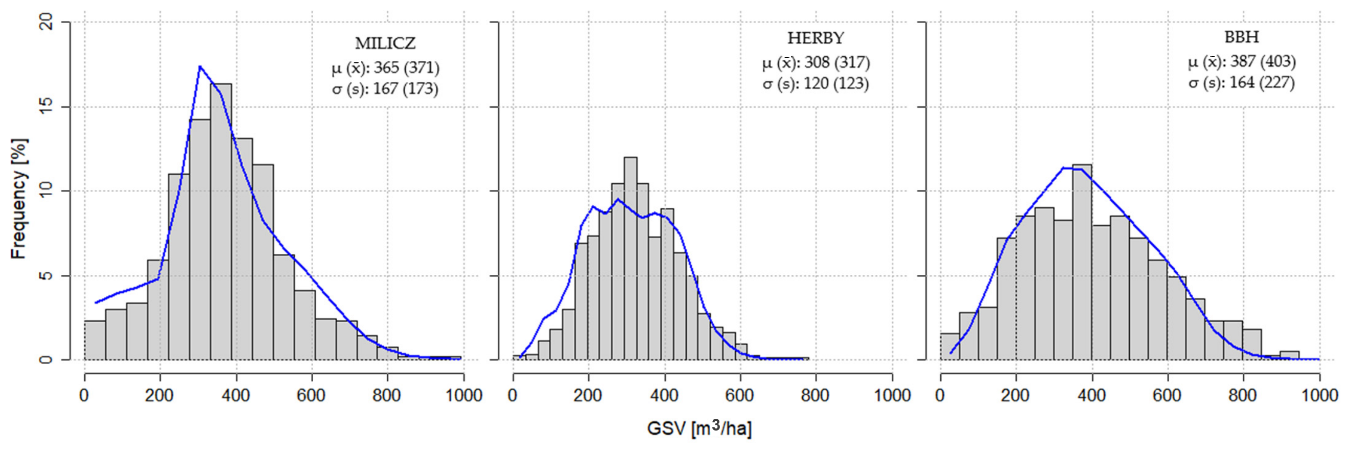
The resulting synthetic GSV was subsequently treated as the reference (“true”) GSV for each grid cell. The mathematical definition of the synthetic target variable is provided in Equation (1), while Figure 3 compares the GSV distributions of the semi-synthetic population and the real forest inventory plots.
where
- Vi—synthetic GSV for ith grid cell;
- fXGB()—basic XGBoost GSV prediction for ith cell;
- xi—vector of predictor variables for ith cell;
- N3(i)—3 nearest real inventory plots to ith synthetic plot/grid cell in multidimensional data space;
- Vs—observed GSV of sth real inventory plot;
- —LOO-XGBoost GSV prediction for real sth plot;
- us—random multiplicative perturbation, where us ~ U(−0.05, 0.05).
Figure 3.
GSV distributions according to real forest inventory data (grey bins) and synthetic response (blue line). Mean and standard deviation were provided for synthetic population and inventory data (in brackets).
2.5. Sampling Designs
The performance of three sampling designs was evaluated in this study: simple random sampling, systematic sampling, and stratified sampling, each examined under multiple variants (scenarios). The grid cells described in the previous section were used as the basic sampling units. The efficiency of each sampling design was evaluated based on the mean normalized BIAS and normalized root mean squared error (RMSE) across simulation scenarios that differed in terms of: sample selection method, sampling intensity, estimator type, and availability of auxiliary variables. For sampling designs incorporating an inherent stochastic component, namely SRS and SYS, 100 iterations were performed to assess the variability of the resulting estimators.
Uniform-probability simple random sampling without replacement was tested in its most basic form. For each forest district in each systematic sampling scenario, a rectangular sampling grid was overlaid on the study area 100 times. Sampling intervals ranged from 100 to 2000 m. However, only scenarios resulting in a maximum sampling intensity of 1000 plots or fewer were further considered. To preserve the statistical validity of the systematic sampling design, SYS was implemented using both a random starting point and a random grid orientation [116].
Hierarchical agglomerative clustering using the Ward.D linkage method [57,117], implemented through the hclust function in the fastcluster R package (v. 1.3.0) [118], was used to group sampling units in StrS. A previous study [58] demonstrated the particular suitability of this algorithm for stratifying forested areas based on ALS metrics. Instead of Euclidean distances, Gower’s coefficient [119], implemented in the daisy function of the cluster R package (v. 2.1.4) [120], was used to determine pairwise dissimilarities for clustering, as some scenarios included non-numerical auxiliary variables, such as tree species information. Owing to computational and memory limitations imposed by the software packages used, a random subset of sampling units (grid cells) was selected for clustering and actual sample selection, whereas GSV predictions and error estimation were performed using the full populations. Appendix D compares the main characteristics of the response variable distributions in the full semi-synthetic populations and their reduced counterparts. Given the similarity between these distributions, we expect this reduction to have had, at most, a marginal influence on the final results.
For StrS, three methods of allocating the sample size among strata were evaluated: allocation proportional to stratum size (Size), allocation proportional to stratum variance (Var), and Neyman’s optimal allocation (NOA) [121], which accounts for both factors. Within-stratum variability was evaluated using only the auxiliary variables available in a given scenario. For numerical variables, the coefficient of variation was calculated, whereas for categorical variables, normalized Pielou’s evenness was derived from Shannon entropy [122,123]. For each stratum, a weighted mean of the aforementioned variability measures was calculated, using the RF variable importance index as the weighting factor [103].
For within-stratum sample selection, three methods were evaluated: random selection (RAN), nearest-centroid selection (NC) akin to [54], and regular in-data-space sampling (REG). Before applying NC and REG within each stratum, all variables were standardized using z-scores (mean-centering and standard deviation-based scaling) to prevent biased sample selection resulting from differences in the scales of individual auxiliary variables.
For each stratum under REG, the stratum centroid was calculated as a vector of mean values across all numerical auxiliary variables available in a given scenario. Subsequently, the Euclidean distance between each sampling unit in a given stratum and the centroid was calculated. The range of distances was divided into equally spaced intervals based on the sample size allocated to the respective stratum. The sampling unit closest to each successive interval boundary was selected, with ties resolved by random selection. When only categorical variables were available, REG selection was based on sorting by sampling unit ID. A pseudocode representation of this procedure is provided in Appendix B.
2.6. GSV Estimation and Evaluation
Two GSV estimators, namely random forest regression and ordinary linear regression, were independently fitted using samples selected according to the procedures described in the previous section.
The RF estimator was used as implemented in R following Breiman’s random forest algorithm [103,124]. This implementation involves a stochastic component and may therefore produce slightly different results across runs. To account for this variability, the RF procedure was repeated 10 times for each REG and NC sampling variants of StrS. No RF repetitions were designed for SRS, SYS and StrS-REG, after observing relative insensitivity of scores between RF runs, and assuming that sampling repetitions should already account for this source of limited variability. Details about the exact numbers of RF runs in particular sampling methods, as well as their lack of practical influence on the variability of the results, are demonstrated in Appendix G. The following RF hyperparameters were used: ntree = 500, mtry = 0.6 × the number of available predictors, and node size = 5. A brief hyperparameter tuning was performed (Appendix E); however, previous studies have reported that these parameters generally have a relatively limited influence on model performance beyond certain threshold values [125,126,127].
The OLR estimator included all predictors available in a given scenario. However, to ensure computational feasibility and avoid the excessive number of possible model specifications, interactions between auxiliary variables were not included in the OLR models. Nevertheless, such interactions are inherently accounted for by RF. In scenarios involving categorical variables, separate linear regression models were fitted for each group. When only categorical variables were available, the arithmetic mean was used as the estimator for each respective stratum.
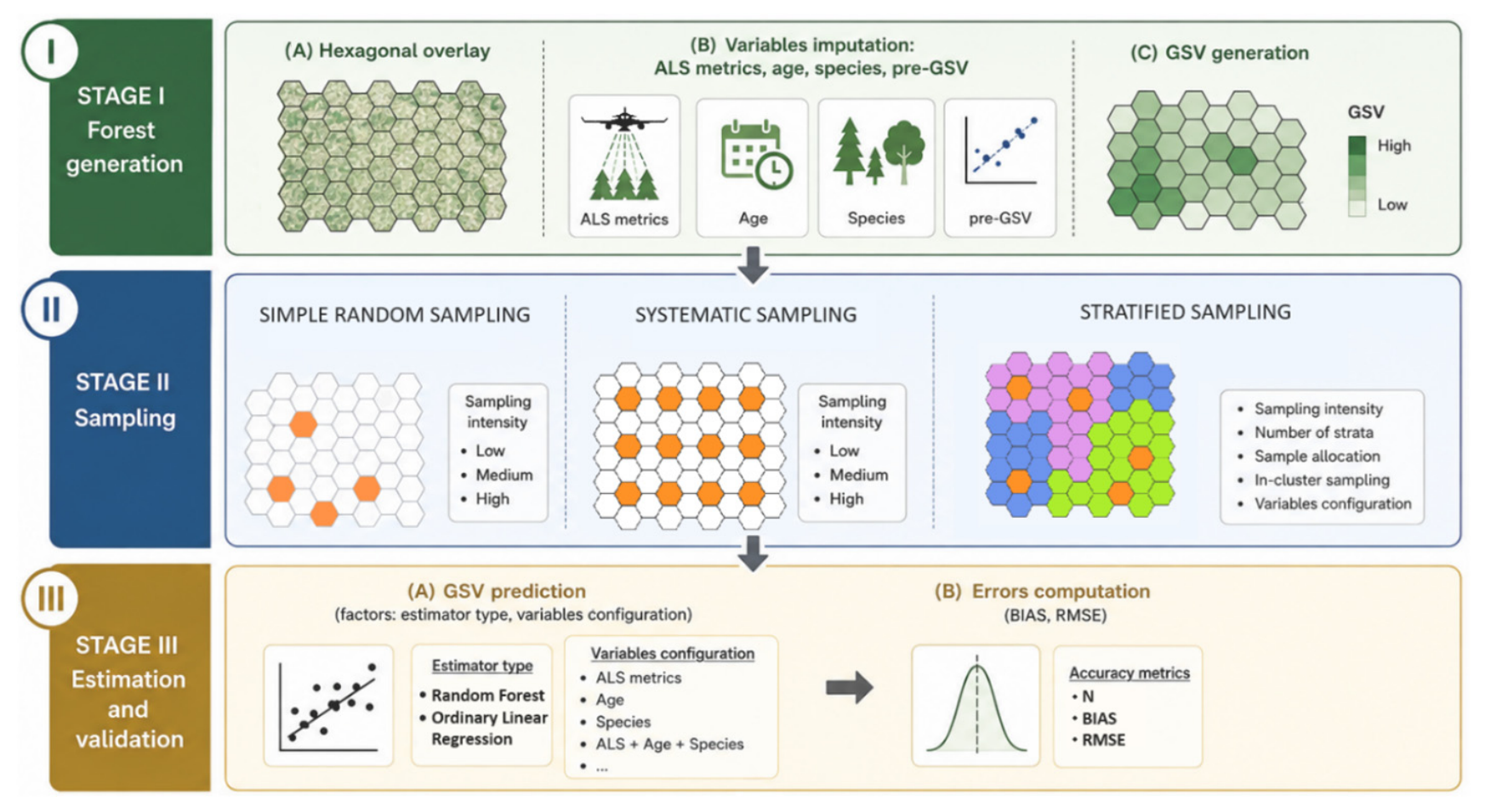
No outlier treatment was applied at this stage. The complete set of selected samples was used for model fitting and subsequent GSV prediction in every scenario. Given that model-based forest populations tend to simplify distributions (Figure 3) [88,89], we assumed that this effect would have a limited influence on our study design. In every scenario, the models resulting from each iteration were used to predict GSV for all hexagonal grid cells representing the units of the semi-synthetic forest population. The performance of each model instance in every scenario was evaluated using mean normalized BIAS (Equation (2)) and normalized RMSE (Equation (3)), calculated across the entire population, with grid cells treated as individual observations. Figure 4 provides a graphical summary of the overall methodological framework.
where
- —estimated GSV value for i-th grid cell;
- yi—reference GSV value of i-th grid cell;
- n—number of observations (grid cells);
- μ—population GSV mean.
Figure 4.
Graphical summary of the methodology.
3. Results
In this section, each forest inventory method is first examined separately to reduce the multidimensionality of the analysis and identify the most suitable variants. The final subsection compares the most promising variants across all sampling methods.
3.1. Simple Random Sampling
Under this sampling design, ALS metrics alone resulted in the lowest estimation errors in most cases (Table 4 and Table 5). Adding GM pre-estimates slightly reduced RMSE and BIAS in some cases; however, the improvements were marginal, amounting to only 1–2 pp. When used alone, stand age or species information resulted in substantially higher estimation errors, particularly at lower sampling intensities. Combining these variables with ALS metrics or GM pre-estimates resulted in only marginal improvements, again of approximately 1–2 pp. Differences between the RF and OLR estimators in terms of GSV estimation errors were negligible in most SRS configurations. However, at lower sampling intensities, OLR tended to produce slightly lower error values than RF, whereas the opposite pattern was observed at higher sampling intensities. This observation is consistent with the general understanding that machine learning methods typically require larger sample sizes than conventional regression models to produce stable estimates [128,129,130]. Regarding the influence of sampling intensity under SRS, the results suggest that the convergence zone for the most effective configuration, i.e., ALS predictors combined with the RF model, occurs at approximately 150–200 plots (Figure 5 and Figure 6).
Table 4.
BIAS scores in particular configurations of SRS (the highest error from 100 iterations).
Table 5.
RMSE scores in particular configurations of SRS (the highest error from 100 iterations).
Figure 5.
BIAS of selected SRS configuration: ALS predictors, RF estimator (the highest error).
Figure 6.
RMSE of selected SRS configuration: ALS predictors, RF estimator (the highest error).
3.2. Systematic Sampling
Table 6 clearly indicates that the choice of estimator in the two-phase systematic sampling design was of secondary importance for GSV estimation in SYS. At all sampling intensity levels, the differences in BIAS between the two estimator types did not exceed 0.2 percentage points (values in brackets). In contrast, a slight improvement in RMSE, of up to 2.2 percentage points, was observed when RF was used as the GSV estimator, particularly at higher sampling intensities. These results provide further evidence that RF models can benefit from larger sample sizes [131]. Given the slight advantage of RF as a GSV estimator, the subsequent analysis focuses primarily on this estimator.
Table 6.
Most efficient types of estimators in systematic sampling.
Table 7 presents the performance of the RF estimator under systematic sampling for different combinations of auxiliary variables used for GSV prediction. The main purpose of this analysis was to narrow down the number of possible variable combinations and identify the most promising ones. In most cases, ALS predictors resulted in the lowest RMSE values, whereas BIAS remained relatively stable across the different configurations, possibly due to the averaging of estimates. Adding preliminary GSV estimates from the generic model slightly reduced mean RMSE values by up to 1–2 percentage points (pp) in the Herby and Milicz forest districts, which exhibited lower structural complexity than BBH. The addition of other auxiliary variables did not substantially improve estimation accuracy. Using only stand age or species information resulted in considerably higher RMSE values and slightly higher BIAS, with differences of up to 3 pp observed mainly at lower sampling intensities.
Table 7.
RF in SYS efficiency, BIAS% (RMSE%), across all variable config. (mean absolute values over 100 iterations).
The lines in Figure 7 and Figure 8 illustrate the worst-case performance of the RF estimator under SYS for GSV prediction in a two-phase forest inventory using only ALS metrics. They represent the worst results observed across 100 iterations at each sampling intensity level. The highest estimation errors were observed in BBH, whereas the lowest were recorded in Herby and Milicz, which exhibited similar performance. This pattern corresponds well with the structural complexity of the respective study areas. BIAS values stabilized at approximately 400 sample plots (Figure 7), whereas RMSE values reached a plateau somewhat earlier, at approximately 300 plots, across all study areas (Figure 8).
Figure 7.
BIAS of selected config. of SYS: ALS variables, RF estimator (the highest errors).
Figure 8.
RMSE of selected config. of SYS: ALS variables, RF estimator (the highest errors).
3.3. Stratified Sampling
Table 8 and Table 9 show the distributions of absolute BIAS and RMSE values for selected configurations of the stratified sampling design. These results are based exclusively on ALS variables, as their suitability for GSV prediction was confirmed in Table 10. Again, the RF estimator showed a slight advantage over OLR in some configurations. Among the variants considered, one configuration (highlighted in aquamarine) provided consistently low and relatively stable BIAS values, regardless of the study area or sampling intensity. This configuration combined Neyman’s optimal allocation (NOA) of the total sample size among strata, regular in-data-space sampling (REG), and RF as the GSV estimator. Similar performance was achieved using sample allocation proportional to stratum size. However, at lower sampling intensities, this approach was less stable than the selected configuration, resulting in BIAS values of up to 4% in the Milicz forest district, compared with consistently observed values of 1–2% across all study areas for the selected configuration.
Table 8.
BIAS distribution [%] for selected configurations of StrS (worst score from all iterations).
Table 9.
RMSE distribution [%] for selected configurations of StrS (worst score from all iterations).
Table 10.
Influence of variable types for GSV estimation in selected configuration of StrS.
Based on the visual inspection of Table 9, the RMSE scores were less susceptible to the sample allocation method than to in-cluster sampling (ICS). The NC usually provided the worst scores, whereas RAN and REG were competitive, with a slight advantage for REG.
Table 10 presents observed upper limits of BIAS and RMSE in StrS, using RF as the GSV estimator, considering different sets of variables used for stratification, NOA/REG sample selection and GSV prediction. The results indicate that ALS variables alone provided the most robust and stable performance across sampling intensity levels and forest districts. Their use maintained BIAS at a consistent level of approximately 1% and yielded relatively low RMSE values, ranging from 13% in Milicz to 18% in BBH. Adding other types of auxiliary variables, such as preliminary GSV estimates from the generic model or stand age and species information, resulted in further reductions in RMSE of up to 2 percentage points (pp) in some scenarios. However, these additions could also introduce additional noise and consequently increase BIAS by up to 2 pp in some cases. Table 10 further indicates that including more than two types of auxiliary variables generally provided no additional benefit and could even be detrimental, potentially due to increased data dimensionality, collinearity, and additional noise associated with the inclusion of further variables and their quality. Most importantly, all configurations that excluded ALS metrics resulted in noticeably higher estimation errors.
Figure 9 illustrates the influence of the number of strata on GSV estimation performance under selected stratified sampling configurations at different sampling intensities. The trend lines represent power functions fitted to the scores obtained across all iterations within each scenario. Figure 9 suggests a convergence zone at approximately 150–200 sample plots. Above this range, no practically meaningful differences in performance were observed, whereas below this threshold, the results appeared to be more strongly influenced by random variation and other unexplained effects, making it difficult to draw consistent conclusions. For example, at lower sampling intensity levels, the BIAS results showed distinct patterns across individual forest districts, depending on the number of strata.
Figure 9.
Influence of the number of clusters on performance of selected StrS configuration: 3—green; 9—orange; 15—blue.
As the results demonstrate, several StrS configurations produced competitive results, with slight variations across study areas. To reduce the dimensionality of the analysis and facilitate a clear and concise comparison of the tested sampling designs, we ultimately selected one preferred StrS configuration. Based on a visual inspection of Table 8, Neyman’s optimal allocation combined with regular in-data-space sampling was selected. The results presented in Table 10 indicated that ALS variables alone were the most suitable predictors for GSV estimation. A slight advantage of the RF estimator over OLR was also evident in Table 8 and Table 9. Finally, three strata were selected, as their number had only a limited influence on estimation performance when the sample size exceeded approximately 150–200 plots (Figure 9).
3.4. Direct Comparison
Figure 10 provides a direct comparison of the analyzed sampling methods using the selected configurations. The results represent the least favourable iteration in each scenario, i.e., the largest estimation error observed across the finite set of simulation runs. At medium and higher sampling intensities (approximately 250–300 plots and above), the choice of sampling design was of secondary importance for GSV estimation in the two-phase, model-based, ALS-assisted forest inventory. In particular, the results indicated that increasing the sample size beyond approximately 300 plots provided little practical benefit. However, at lower sampling intensities, particularly around 100 plots, the advantage of the proposed StrS configuration (green line) became more pronounced, as reflected by its relatively stable BIAS and RMSE values. Notably, this advantage was more evident in structurally complex forest districts, such as BBH and, to a lesser extent, Milicz, than in areas consisting predominantly of relatively simple stands, such as Herby. Apart from StrS, SRS and SYS exhibited relatively similar performance across the entire range of tested sampling intensities.
Figure 10.
Direct comparison of GSV estimation performance across selected variants of SRS, SYS, and StrS. The highest estimation errors observed across all iterations. SRS—blue line; SYS—orange line; StrS—green line.
Figure 11 and Table 11 and Table 12 present the assessment of uncertainty associated with GSV estimation under the different sampling designs. For SRS and SYS, standard deviations (Equation (4)) and standard errors (Equation (5)) were calculated from BIAS and RMSE values obtained across 100 independent sampling iterations. In the selected StrS configuration, the only source of limited variability was associated with the stochastic component between 10 RF runs. Details about the exact numbers of RF runs in particular sampling methods, as well as their marginal influence on the variability of the results, are demonstrated in Appendix G.
Figure 11.
Standard deviation (SD) of BIAS and RMSE for selected configurations of sampling methods: SRS—blue line; SYS—orange line; StrS—green line.
Table 11.
Standard error (SE) of BIAS [pp] for selected config. of sampling methods.
Table 12.
Standard error (SE) of RMSE [pp] for selected config. of sampling methods.
The observed trends were similar for SRS and SYS across all forest districts. Except at very low sampling intensities, SD values remained relatively stable (within 1–2 percentage points) across all sampling designs. However, the variability of BIAS under StrS was slightly lower and stabilized at a sample size of approximately 200 plots (Table 11). At this sampling intensity, the variability of RMSE was similar across all investigated sampling designs (Figure 11, Table 12). Overall, the selected StrS configuration provided more stable estimation errors than SRS or SYS at lower sampling intensities, as the stochastic component of this configuration was minimized. The differences between sampling designs were more pronounced at lower sampling intensities and were more evident for BIAS than for RMSE.
where
- SD—standard deviation of BIAS/RMSE scores from particular iterations;
- SE—standard error of BIAS/RMSE scores from particular iterations;
- xi—single BIAS/RMSE score;
- —arithmetic mean of BIAS/RMSE scores from particular iterations;
- n—number of iterations in the given sampling method:
- SRS = 100, SYS = 100, StrS RAN = 50, StrS NC = 10, StrS REG = 10.
4. Discussion
4.1. General Trends
This study demonstrated the potential of ALS-based, structurally guided sampling for low-sampling-intensity forest stock inventories. In StrS, the convergence zone appeared at smaller sample sizes than in SRS or SYS (Figure 10). This effect was even more pronounced in the structurally more complex study area. For instance, in a relatively simple forest district such as Herby, the differences in error values between sampling methods were up to about 2 pp. However, in a more complex study area, such as BBH, the differences at lower sampling intensity levels, i.e., approximately 100 plots and below, could be as high as ~4 pp, representing a notable improvement relative to the average range of observed errors. On the other hand, the range of RMSE values was slightly higher in BBH, and any improvements are usually more visible at higher error levels. Therefore, validation in at least one or two even more complex forest districts would be desirable to strengthen this hypothetical effect. Further increases in sample size resulted in limited and non-proportional gains in GSV prediction accuracy (up to 2 pp). This trend was characteristic of all analyzed methods. In fact, beyond approximately 200–300 plots, the choice of sampling method appeared to become of secondary importance for GSV prediction performance (Figure 10) [80].
4.2. Limitations
The study design was oriented towards a single-response survey, with GSV as the sole target variable. As noted by [132], unequal-probability sampling approaches, such as SGS, can be efficient for single-response surveys but may not necessarily be optimal for multipurpose forest inventories. Therefore, drawing separate SGS samples for individual response variables and comparing their efficiency with that of a single multipurpose sampling design would certainly merit further investigation. On the other hand, GSV, or closely related biomass, is among the most important forest attributes to be determined in forest management and (NFIs) [133,134,135]. Moreover, other forest attributes, such as DBH or tree height, are often treated as auxiliary, substitute, or intermediate variables [136] and may require smaller sample sizes than GSV when considered as target attributes [68]. Finally, with the widespread use of RS techniques, attributes such as tree or stand height can often be estimated with substantially lower errors than GSV [68] or even measured directly from ALS data [66], in some cases with greater accuracy than conventional ground measurements [65].
The results of this study were presented at the forest-district level. The authors did not plan comparisons of the performance of the selected sampling methods within predefined stratification layers, as is the case in many practical forest inventories [34,36,37,137,138,139]. Such an investigation would require a significant extension of the already broad study. It is therefore possible that the results could vary among post-stratified subpopulations and that optimal sampling could consequently be applied separately within each user-defined stratum. On the other hand, the architecture of the SGS method should inherently account for naturally occurring subpopulations and thus provide a well-balanced sample distribution, irrespective of the complexity of the surveyed area [38]. Therefore, the results were presented for three distinct forest districts. Nevertheless, if population totals and/or means are the sole quantities of interest, for example, in less structurally complex areas, monocultures, or plantations, this issue may be of lesser importance. However, from a broader scientific perspective, this aspect should remain within the scope of further analysis, particularly given that recent European policies increasingly emphasize the conservation, restoration, and enhancement of forest biodiversity [140,141,142].
Although the overall BIAS and RMSE levels were relatively small, it should be remembered that the results were evaluated against a semi-synthetic response variable, and model-generated outputs often tend to provide smoother and less complex representations of real populations [88,89]. As shown in Figure 3 and Table 9 (RMSE), the present study was no exception in this regard. Therefore, the results presented here should be treated as indicative of general trends rather than as definitive guidelines. Nevertheless, the conditions were identical for all tested sampling methods and, in accordance with the objectives of the study, the relative differences in performance between the investigated methods were more important than the absolute error values. In the presented simulations, the authors tried to imitate real inventory cases as closely as possible. However, in practice, sampling is performed only once. Therefore, it is desirable to know the approximate range of possible error characteristics associated with the considered sampling methods. For practical reasons, in our opinion, the limited influence of the stochastic element specific to the presented StrS/SGS method is a major benefit compared with SRS and SYS, where their randomness must often be balanced by increasing the sample size. Therefore, in addition to the standard deviations of RMSE/BIAS scores (Figure 11) and standard errors (Table 11 and Table 12), the final results presenting direct comparisons between the investigated sampling methods also include the largest error observed within a finite set of repetitions in a given scenario (Figure 10). On this occasion, the authors would like to highlight that GSV estimates from real stand-level inventories were used as auxiliary predictors for the generation of the reference GSV values. This constitutes an additional reason for treating the generated forests as semi-synthetic populations.
4.3. Complex Sites and Additional Variables
Although the selected study areas were characterized by relatively diverse species composition and structural complexity (with regard to Polish lowland environmental conditions), no mountainous regions were included in the analysis. This was mainly due to the lack of hyperspectral data and, consequently, sufficiently detailed species information for mountain regions, which was necessary to create reliable semi-synthetic forest populations. However, based on the results presented in Figure 10, perhaps complex sites (akin to BBH) could benefit more from SGS than homogeneous sites, although this broad premise definitely requires additional testing across more sites with varying characteristics.
Under the discussed conditions, SGS could potentially utilize additional variables, such as site characteristics, climatic drivers, slope, aspect, elevation, and XY coordinates, to achieve more effective sampling than SRS or SYS. Nonetheless, a substantial impact of these auxiliary variables should not necessarily be expected, as even predictors more strongly correlated with GSV and used in this study, such as stand age and species composition, generally did not improve the results substantially once ALS metrics were available (Table 10). This result suggests that the exclusive use of ALS metrics can already explain most of the variance in GSV. Height metrics, in particular, were usually the most strongly correlated with tree and stand volume (Appendix F). Perhaps these limited improvements could also be partially explained by the authors of [143], who demonstrated a method incorporating species information into ALS-based GSV prediction models. That method reduced RMSE by 2 to 9 pp. Nonetheless, in their research, the additional species information was also derived from ALS data. Similar observations were reported by [37], who clearly stated the need to replace species information with other auxiliary variables for stratum delineation, having found a low correlation between species information and GSV (0.12).
Similarly, information on stand age could not visibly improve the overall BIAS and RMSE scores. If present, gains of up to 1–2 pp were more often observed at medium and higher sampling intensity levels. However, the addition of species data was usually more informative. This result can be partially explained by the naturally higher autocorrelation between ALS height metrics and stand age than between ALS height metrics and species data. Moreover, increasing the dimensionality of the auxiliary data space at lower sampling rates could be another source of uncertainty and instability in RF-derived GSV estimates. For instance, ALS or ALS + SP/AGE could be more informative configurations of StrS than ALS + SP + AGE when using 100 plots for model calibration (Table 10). Another explanation for the noisy/unstable behaviour following the addition of age information could be that stand age was assigned based on the dominant group of trees across the entire stand. Theoretically, individual stands should be delineated in a way that ensures the most structurally homogeneous conditions [34]. However, in practice, such distinction is usually challenging, especially when accounting for the vertical structure of multilayered stands, as individual stands can be very heterogeneous in terms of, for instance, age information and species composition across different layers. We would also like to note that the accuracy of age estimation was not reported by the data provider.
Furthermore, ref. [144] found little influence of climatic drivers and site conditions on tree-level volume estimates when these variables were combined with ALS metrics. On the other hand, potential latent effects and interactions should always be considered. For instance, ref. [127] demonstrated that slope had no meaningful influence on GSV estimates, either for the entire sample or for particular groups, with the exception of deciduous stands. This effect was most likely related to reduced DTM accuracy resulting from the weaker penetration of LiDAR signals through the denser crowns of broadleaved tree species.
4.4. Ex Situ Data
Preliminary GSV estimates obtained from generic models trained exclusively on ex situ data were not as attractive as initially presumed. One possible explanation is that the performance of ex situ models could have been improved if spatial autocorrelation had been explicitly taken into account. On the other hand, ref. [58] demonstrated little evidence of spatial autocorrelation among mostly managed forest districts in Poland. Moreover, for the relatively small forest areas considered in this study, the effect in question could be reduced even further [145]. Regarding the spatial separation between sites, ref. [146] found ex situ models to be competitive with local forest inventories within a 100 km range; however, the distances between some of the forest districts in our study could have been slightly greater. In contrast, Table 5, Table 7 and Table 10 suggest that, wherever possible, ALS in situ models should be preferred, as they naturally provided better results than models based exclusively on generic ex situ information. This finding is in agreement with the results of [147], who concluded that at least some number of local plots should always be secured for model calibration, or at least for controlling the magnitude of possible estimation errors. Quite surprisingly, ref. [146] found that only 20 in situ plots, selected using SRS, might be sufficient to calibrate external models in such a way as to provide precision and accuracy levels comparable with those of a new local inventory. Nevertheless, the authors of that study used relatively small datasets, resulting in unusually high sampling intensity rates. To mitigate that effect, the authors used replacements for sample plot selection. Regarding the spatial scale, ref. [148] obtained the best performance when training plots were limited to a 20 km radius, although the results were based on Landsat TM data. Based on the results presented in our study, the provision of preliminary GSV estimates as auxiliary predictors for in situ calibrated models could improve the results by only approximately 1–2 pp across all sampling methods (Table 5, Table 7 and Table 10). Such an approach bears some affinity to stacking ensemble architectures, which seek to leverage the complementary advantages of predictions derived from separate models or data sources [149,150,151,152]. Nevertheless, in most cases, ALS + GM scenarios produced BIAS and RMSE values similar to those achieved by models utilizing only in situ ALS metrics. Moreover, additional caution may be warranted when using ex situ information, as in some cases, GM metrics combined with other predictors produced slightly inferior results compared with scenarios in which different metric types were used separately. Possibly, the introduction of additional variables may have induced some extra noise related to multidimensionality and/or the quality of certain auxiliary variables. For instance, the inclusion of either stand age or species information could visibly improve GM performance in StrS. This behaviour could be partially explained by the fact that SGS can utilize additional data to a greater extent than SRS or SYS. However, quite interestingly, when age and species information were combined with GM, the aforementioned gain was observed to a lesser extent (Table 10). Obviously, the conducted analysis cannot exclude other possible causes of the observed patterns. The inclusion of ex situ data from generic models constituted only a secondary aspect of this study, rather than its main objective. Therefore, based on the current analysis, it is challenging to draw firm conclusions about these contingencies. The plausible causes of this behaviour remain to be investigated in further analyses.
4.5. Practical Implications
In general, the obtained results followed rather logical expectations. Flexible stratification based on population parameters can facilitate the minimization of within-group variance and differentiation between groups, which, in turn, can result in a more optimal and well-balanced sample distribution. In SRS, as well as in SYS, the stochastic element plays a crucial role in practical realizations, whereas in the proposed SGS, the random component is kept to a minimum, with the RF iterations being its main source. This aspect can be considered a meaningful practical benefit of StrS/SGS. It was also one of the reasons for preferring hierarchical clustering over k-means partitioning, as the former, when combined with Ward linkage, has been shown to be more stable than the latter [58]. Nevertheless, the observed randomness could potentially be reduced even further by using OLR instead of RF as the estimator. In fact, linear regression performed slightly better than RF in some scenarios, particularly at lower sampling intensity levels. This observation is consistent with the general tendency of machine learning techniques to require larger sample sizes than OLR to achieve stable predictions [128,129,130]. Nonetheless, the predictive performance of GSV estimation was similar for both estimators, with differences of up to approximately 1–2 pp and a slight advantage of RF in the majority of scenarios.
Based on the observed results, some practical recommendations can be formulated regarding the choice between OLR and RF for GSV estimation. Namely, given a very small sample size, OLR appears to be the more stable choice. At larger sample sizes, RF seems to be preferable, as it can provide a slight improvement in predictive performance. Compared with linear regression, RF is generally less sensitive to the inclusion of irrelevant or noisy predictors. Moreover, it inherently accommodates non-linear relationships and interactions between predictors, thus reducing the need for rigorous a priori variable selection and the formulation of an explicit model equation [124,153,154]. In the case of OLR, both the model formula and potential interactions must be explicitly specified, which can drastically increase the number of possible model configurations.
We would also like to stress that, in this research, the same model was used for each stratification group. The application of stratum-specific models could potentially contribute to a further reduction in error rates. Although RF and OLR produced comparable results, only two types of estimators were tested in this study. The literature remains ambiguous regarding the selection of the most appropriate estimator. Similarly to the present study, ref. [155] found little influence of the prediction method (up to 3 pp), whereas other studies reported quite contrary results. For instance, ref. [80] showed a notable influence of the prediction method on the required sample size, favouring RF over other methods when the target precision level was set to a 5% standard error. Ref. [131] also supported the use of RF for biomass estimation over other prediction methods, such as kNN, SVM, OLR, or Gaussian Processes. This aspect certainly warrants further investigation, as positive results could indicate that, under certain circumstances, the use of ALS metrics might become redundant. As a further consideration, if only approximate population totals or means were of interest, regardless of the local spatial variability of the response variable, data from previous inventories could be reused in managed forest districts. For instance, according to Table 4 and Table 10, when only stand age information was used for GSV prediction based on 500 observations, some BIAS values fell within a reasonable range of approximately 2–4% at the forest district level.
While the proposed StrS approach outperformed SRS and SYS at lower sampling intensity levels, it is generally more complex and may therefore require additional preparation. Several issues should be considered before implementing StrS: (1) the required level of accuracy or available sample size, (2) the selection of appropriate auxiliary variables for stratification and/or sampling, (3) the selection of adequate stratification rules, (4) the allocation of sample sizes among strata, (5) the within-stratum sampling design, and (6) preferences regarding the type of estimator. Moreover, the potential interactions among these factors and the consequences of their particular combinations should always be taken into account. The above considerations were the main motivations for undertaking the present study. The authors sought to approximate the expected inventory error rates associated with decisions regarding the selection of sampling methods and their respective variants.
The results showed that structurally guided stratification of ALS metrics can help distinguish meaningful subpopulations within heterogeneous forest districts. Although only one “stratification engine” was employed, namely hierarchical agglomerative clustering with Ward.D linkage, previous research has identified this clustering approach, as well as k-means or k-medoids, as potentially suitable for GSV-oriented forest inventories [36,58,156]. Nevertheless, SGS can also be driven by other “engines”, including the Cube Method [51], the Local Pivotal Method (LPM) [53], and Latin Hypercube Sampling (LHS) [157]. Their suitability for FMI warrants further investigation, as previous studies have indicated the considerable potential of these SGS algorithms for sampling optimization. For instance, ref. [19] reported that LPM can be more efficient than SYS for certain variables in NFI, while [48] demonstrated that LPM and LHS could substantially improve sampling efficiency compared with SRS. However, GSV was not among the forest attributes examined in the latter study.
4.6. Selected Variants
Regarding the StrS configuration, as might be expected, the Neyman allocation method showed considerable potential for achieving a well-balanced sample distribution, as it combines the advantages of the two other sample allocation methods evaluated in this study, namely allocation proportional to stratum size and allocation proportional to stratum variance. Although differences in error scores due to the allocation methods were relatively subtle, Neyman allocation combined with regular in-data-space sampling and the RF estimator consistently maintained relatively low BIAS values, even at limited sample sizes and across all study areas (Table 8). Random in-stratum sampling yielded similar RMSE results but slightly higher BIAS values and was, as expected, somewhat less stable than the regular sampling approach. Nearest-centroid selection produced the highest error values in most scenarios with low sampling intensity, most likely because it failed to adequately represent the full range of variability within the subpopulations.
Interestingly, the choice of k, i.e., the number of clusters/strata, had no major impact on the results at medium and higher sampling intensity levels (Figure 9, Table 8 and Table 9). Although relatively small, differences associated with the number of clusters became apparent only at low (~100) and very low (~50) sampling intensity levels, reaching approximately 2–3 percentage points (pp.). At larger sample sizes, the influence of this factor was negligible. With regard to BIAS, however, different numbers of stratification groups resulted in varying error levels across the study areas, with differences reaching up to 4 pp at lower sampling intensities. No clear pattern could be identified that would allow the optimal number of clusters to be determined. As demonstrated by [156], this may be a highly complex issue and was therefore considered beyond the scope of the present study. Nevertheless, future research aimed at exploring further reductions in sampling intensity should include a thorough investigation of this behaviour. Meanwhile, the present results provide possible justification for avoiding very low sampling intensity levels.
Even though many variants of the selected sampling designs were tested in this study, by no means were all available sampling methods covered. In order to maintain a clear and well-organized research framework, the authors focused on what are perhaps the most common sampling designs [158], supplemented by one relatively new approach which, based on previous research [35,38,46,57,80,137], had shown promising results and therefore appeared worthy of further testing and development. First, SCS was not tested, although it is a very popular design in many national forest inventories [27,28]. This sampling technique is considered particularly useful for NFIs, as it provides a compromise between statistical efficiency and the economic considerations associated with repeated inventories over large areas, such as at the national level. For this reason, it may be less common in forest district inventories. Moreover, under specific circumstances, SYS can be perceived as a special case of systematic cluster sampling [43,159,160], and therefore, drastically different results should not necessarily be expected. Second, ADA initially appeared to be a promising option worthy of analysis in terms of its suitability for forest inventory. However, preliminary tests showed poor performance, particularly at lower sampling intensities, and the approach was therefore omitted from the final analysis. This poor performance could likely be attributed to the fact that, in the briefly tested ADA implementation, the newly selected sample plots at each recursion tended to fall on so-called “hard points”, i.e., areas characterized by higher variance that were generally not representative of the entire population. Perhaps combining ADA with SYS and CS could mitigate the weaknesses of the basic ADA approach and contribute to further optimization of forest inventory designs [43].
In this study, the authors focused exclusively on “clean” forms of the analyzed sampling designs. Nevertheless, in practical forest management inventories, the final sampling approach is often a combination of two or more basic sampling designs [133]. For instance, in Poland, one of the most popular and officially recommended approaches to forest management inventory is, in fact, a combination of stratified and systematic random sampling [34]. Additionally, the potential benefits of applying post-stratification to already completed forest inventories should not be overlooked. PS can be particularly useful for less flexible sampling designs and/or inventories based on repeated measurements of fixed sample plots, as it may improve precision without requiring additional observations [161,162]. It may also be suitable for small areas represented by a limited number of sample plots [163]. An important consideration in PS is that the quality of stratum delineation can substantially affect its efficiency [161]. Moreover, because strata are defined after sampling has been completed, PS cannot fully exploit the advantages of optimal sample allocation among strata. Another important issue concerns endogenous post-stratification (EPS), in which strata are constructed using predictions from a model calibrated with in situ sample data. Such an approach may lead to substantial underestimation of variance if the dependence between the estimated strata and the sample data is not properly accounted for [164,165]. Finally, EPS-based re-estimation has traditionally been applied to data from large-scale forest inventories, such as NFIs. Nonetheless, ref. [162] recently demonstrated the successful application of EPS in a forest management inventory as well. More generally, combining different sampling techniques at different stages of an inventory may help overcome some of the limitations of their individual “clean” forms. However, there is unlikely to be a universal approach suitable for all inventory situations, and the efficiency of combined sampling designs should therefore also be evaluated under different circumstances.
Finally, one should always bear in mind that the simplicity of a sampling design and the associated statistical inference can often be strong arguments for choosing a particular inventory method. The regular pattern and uniform spatial coverage provided by SYS are particularly appealing to practitioners, making this method a very popular choice [18]. Nevertheless, SGS, as well as combinations of different sample selection methods with increasingly available RS/ALS data, offer vast opportunities for further research, methodological development and optimization, as well as potential practical applications.
5. Conclusions
This study demonstrated the potential of hierarchical clustering for stratification in a two-phase model-based forest management inventory. The proposed stratification approach, combining Neyman optimal allocation with regular sampling in ALS data space, allowed for a noticeable reduction in sample size compared with simple random sampling and systematic sampling, while maintaining relatively low GSV estimation errors at the district level. The preferred configuration of the stratified sampling design produced relatively stable results across all study areas at sampling intensities of approximately 200 plots or more. However, multipurpose inventories and real-world forest conditions would likely require a greater number of field observations. At the investigated sampling intensities, the number of stratification groups had only a limited effect on GSV estimation accuracy, whereas at lower sampling intensities, its influence was more variable.
ALS metrics were the strongest GSV predictors among the variable types tested in this study. Moreover, ALS data constituted the most appropriate basis for the structural stratification of the forests considered. The addition of pre-GSV estimates from generic ex situ models could slightly improve the accuracy and precision of the final GSV estimates. However, at lower sampling intensities, their inclusion could also introduce additional noise, probably due to increased multidimensionality and certain dissimilarities among the inventoried objects. Similarly, the inclusion of species and/or age information did not notably improve the results when combined with ALS variables. When used alone, these variables generally resulted in higher estimation errors, particularly RMSE. Further exploration of different types of variables and methods may bring additional benefits to forest inventories.
Differences between the two estimators were relatively small, with a slight overall advantage of random forest over ordinary linear regression, particularly at higher sampling intensities. At smaller sample sizes, however, ordinary linear regression often produced more stable results. The performance of simple random sampling and systematic sampling was similar across all sampling intensities, indicating that, under the conditions examined in this study, the differences between these two designs were considerably smaller than those observed between either of them and the proposed stratified approach.
Finally, it is important to remember that the results of this study were based on partially simulated data. Such populations tend to simplify the heterogeneity of real forest structures. Therefore, all findings should be treated as approximations of general trends rather than as definitive guidelines. Accordingly, a direct comparison of the proposed stratified inventory design with simple random sampling, systematic sampling, and potentially other sampling methods not tested in this study, using entirely real forest data, would constitute an important direction for future research and provide valuable empirical validation of the findings presented here. In particular, further tests across more diverse study areas, including mountain regions, are needed to better assess the potential of the investigated forest inventory methods. The performance of SGS should therefore be evaluated also at the subpopulation level and in multipurpose forest inventories.
Author Contributions
Conceptualization, M.L.; methodology, M.L.; software, M.L. and K.M.; validation, M.L., K.M. and E.W.-F.; formal analysis, M.L.; investigation, M.L.; resources, M.L. and K.M.; data curation, M.L. and K.M.; writing—original draft preparation, M.L.; writing—review and editing, M.L., K.M. and E.W.-F.; visualization, M.L.; supervision, E.W.-F.; funding acquisition, E.W.-F. All authors have read and agreed to the published version of the manuscript.
Funding
This research received no external funding.
Data Availability Statement
The datasets presented in this article are not readily available because the data are part of ongoing studies. The simulation code constitutes intellectual property of the authors and is a crucial part of other ongoing studies; therefore, it cannot be shared during the duration of these projects.
Conflicts of Interest
The authors declare no conflicts of interest.
Abbreviations
The following abbreviations are used in this manuscript:
| SRS | Simple random sampling |
| SYS | Systematic sampling |
| StrS | Stratified sampling |
| SGS | Structurally guided sampling |
| SCS | Systematic cluster sampling |
| CS | Cluster sampling |
| ADA | Adaptive sampling |
| ALS | Airborne laser scanning |
| RMSE | Root mean square error |
| RS | Remote sensing |
| RF | Random forest |
| OLR | Ordinary linear regression |
| XGB | XGBoost model |
| GSV | Growing Stock Volume |
| SA | Sample allocation |
| NOA | Neyman optimal allocation |
| ICS | In-cluster (stratum) sampling |
| NC | Nearest centroids |
| RAN | Random draw |
| REG | Regular in-data-space sampling |
| GM | Generic model |
| BBH | Białowieża, Browsk, Hajnówka, treated as one object |
| SP | Species information |
| pp | Percentage points |
| ppsm | Pulses per square metre |
| PC | Point-cloud |
| LiDAR | Light Detection and Ranging |
| FMI | Forest management inventory |
| NFI | National forest inventory |
Appendix A. Influence of k Residuals and the Range of Stochastic Perturbations (SPR) on Main Parameters of Semi-Synthetic Populations
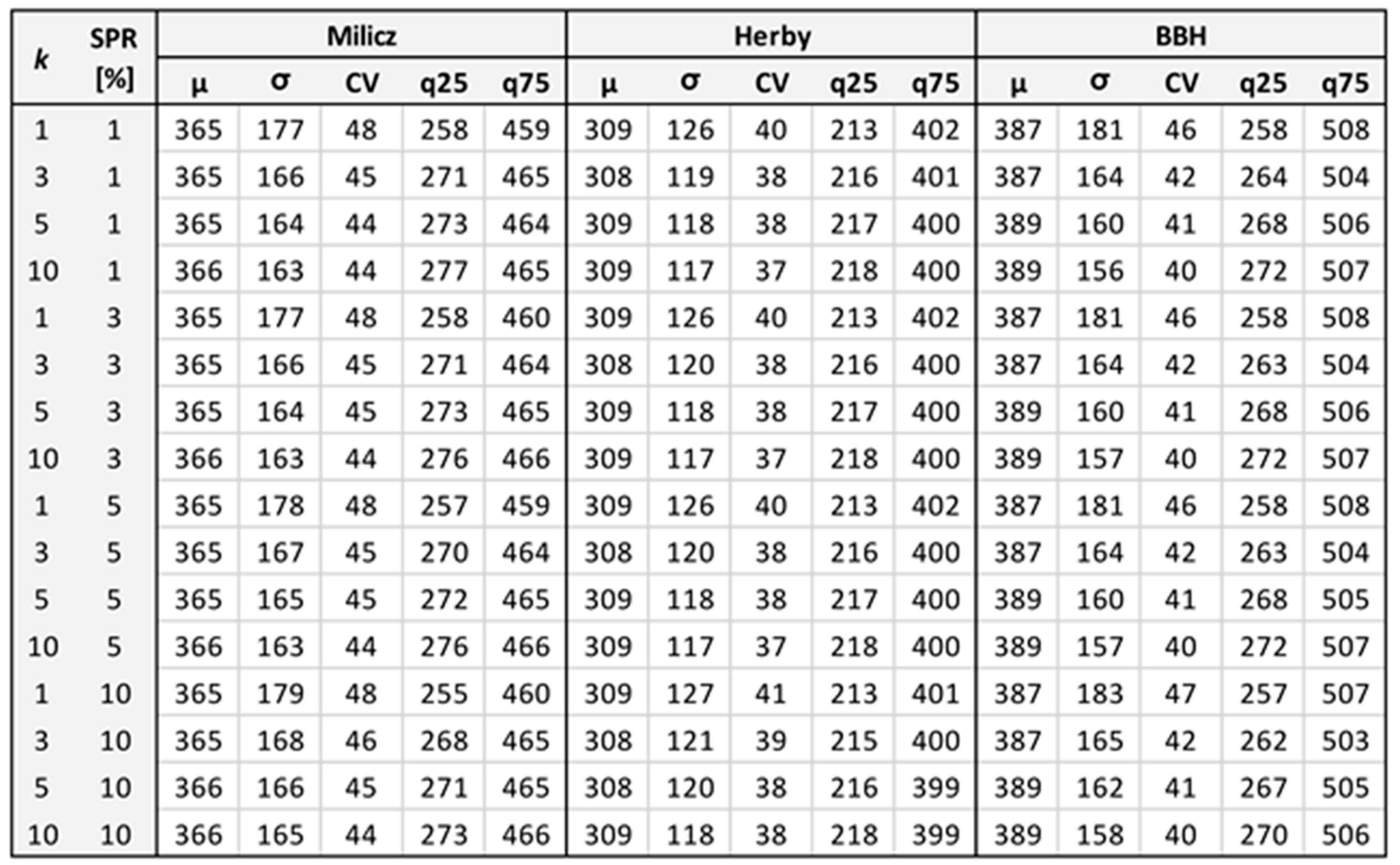
Settings of the hyperparameters used in XGBoost: eta = 0.05, max_depth = 8, min_child_weight = 5, subsample = 1, colsample_bytree = 1, lambda = 1, gamma = 0, nrounds = 2001 (501 for residuals). Non-listed hyperparameters were set to default values. Descriptions of particular hyperparameters can be found in the xgboost library documentation.
Appendix B. Pseudocode for Regular In-Data-Space Sampling
Determine the allocated sample size for all strata.
For each stratum:
If mixed or numerical data types are available:
(Do only for numerical variables)
Calculate the centroid of the stratum.
Calculate each unit’s Euclidean distance to the centroid.
Divide the distance range into equal intervals,
according to stratum-allocated sample size.
For each interval boundary:
Select the unit closest to that boundary.
If tied, randomly select one of the tied units.
Remove selected plot from the sampling units.
Pool the selected units across strata.
If only categorical variable is available,
(There was only one categorical variable in the study):
Assign IDs to each unique value of the categorical variable,
Sort units by the ID,
Enumerate rows,
Calculate interval by dividing max row value by allocated sample size,
Round the interval to integer,
Select 1 unit at every interval boundary.
Pool the selected units across strata.
Appendix C. Software and Libraries Versions Used in the Study
| Software/Library | Purpose | Version |
| R | Main coding environment | 4.3.0 |
| Stats | Cutree and basic statistics | 4.3.0 |
| lidR | ALS data processing | 4.1.1 |
| Fastcluster | Hierarchical clustering | 1.3.0 |
| Cluster | Daisy for Gower dissimilarities | 2.1.4 |
| randomForest | GSV estimation | 4.7-1.1 |
| xgboost | Reference GSV generation | 3.2.1.1 |
| FNN | kNN | 1.1.4.1 |
| sf | Handling of spatial vector layers | 1.0-1.6 |
| dplyr | Tabular/data frame processing | 1.1.4 |
| terra | Handling of spatial raster | 1.7-71 |
| future | Parallel computing | 1.34.0 |
| doParallel | Parallel computing | 1.0.17 |
| Foreach | Parallel computing | 1.5.2 |
Appendix D. Comparison of the Main Parameters of the Response Variable, from Original and Reduced Populations
| District | BBH | Milicz | Herby | |||
| Population | Full | Reduced (10.4%) | Full | Reduced (50.0%) | Full | Reduced (74.1%) |
| Grid-cell count | 627,152 | 65,000 | 106,876 | 53,443 | 67,443 | 50,000 |
| Quantile 0.01 | 74.0 | 72.4 | 26.9 | 25.2 | 60.6 | 60.7 |
| Quantile 0.25 | 264.3 | 264.7 | 266.9 | 266.0 | 215.9 | 216.0 |
| Median | 376.8 | 376.6 | 356.9 | 356.6 | 306.0 | 305.8 |
| Mean | 387.2 | 387.1 | 365.9 | 365.2 | 308.8 | 308.6 |
| Quantile 0.75 | 503.8 | 502.7 | 470.4 | 469.5 | 400.1 | 399.9 |
| Quantile 0.99 | 764.7 | 764.1 | 776.7 | 777.5 | 571.1 | 570.8 |
Appendix E. Influence of RF Hyperparameter Tuning: Values Represent Differences in RF—OLR GSV Means
| Node Size | ||||||||||
| 3 | 5 | 10 | ||||||||
| nTree | N 100 | N 250 | N 500 | N 100 | N 250 | N 500 | N 100 | N 250 | N 500 | mtry |
| 250 | 3 | 1 | −1 | 4 | −1 | 0 | 1 | −1 | 1 | 1 |
| 0 | 0 | 1 | 2 | 2 | 0 | 3 | 0 | 0 | 2 | |
| 3 | 0 | 1 | −1 | −1 | 2 | 1 | 1 | 0 | 3 | |
| 500 | −3 | 2 | 0 | 2 | 1 | 2 | 1 | 1 | −1 | 1 |
| 0 | 2 | 1 | 4 | 2 | 0 | 3 | 1 | 1 | 2 | |
| 1 | 0 | 0 | 3 | 1 | 0 | 5 | 1 | −1 | 3 | |
| 1000 | 1 | 1 | 1 | 2 | 2 | 1 | 0 | 1 | 0 | 1 |
| 4 | 1 | 1 | 3 | 0 | 0 | 1 | 0 | 0 | 2 | |
| 4 | 3 | −1 | 1 | 2 | 0 | 3 | 4 | −1 | 3 | |
Appendix F. GSV-ALS Correlation
| Variable | Dataset | BBH | Milicz | Herby |
| pZbv2_p | population | 0.47 | 0.67 | 0.62 |
| sample | 0.48 | 0.49 | 0.56 | |
| Zmean | population | 0.87 | 0.94 | 0.92 |
| sample | 0.81 | 0.83 | 0.85 | |
| Zq95_p | population | 0.66 | 0.86 | 0.82 |
| sample | 0.68 | 0.70 | 0.75 |
Appendix G. Number of RF Runs in Particular Sampling Methods and Their Influence on the Variability of the Results for Selected Sampling Variants: Example for 100 Sample Plots and the Most Complex Study Area—BBH
| Sampling Method | SRS | SYS | StrS-RAN | StrS-NC | StrS-REG |
| Sampling repetitions | 100 | 100 | 50 | 1 | 1 |
| Actual RF runs per sampling repetition, used for presented results | 1 | 1 | 1 | 10 | 10 |
| Reported BIAS SD [pp] | 1.66 | 1.80 | 2.01 | 0.15 | 0.21 |
| BIAS SD if 30 RF runs had been used [pp] | 1.84 | 1.84 | 2.03 | 0.19 | 0.16 |
| Reported RMSE SD [pp] | 0.68 | 0.56 | 0.87 | 0.17 | 0.07 |
| RMSE SD if 30 RF runs had been used [pp] | 0.71 | 0.58 | 0.94 | 0.15 | 0.06 |
References
- Knoke, T.; Kindu, M.; Schneider, T.; Gobakken, T. Inventory of Forest Attributes to Support the Integration of Non-provisioning Ecosystem Services and Biodiversity into Forest Planning—From Collecting Data to Providing Information. Curr. For. Rep. 2021, 7, 38–58. [Google Scholar] [CrossRef] [Scilit]
- Vatandaslar, C.; Boston, K.; Ucar, Z.; Narine, L.L.; Madden, M.; Akay, A.E. Precision Forestry Revisited. Remote Sens. 2025, 17, 3465. [Google Scholar] [CrossRef] [Scilit]
- Perry, N.T.; Schweier, J.; Bont, L.G.; Kushwaha, S.K.P.; Peltola, H.; Eyvindson, K.; Astrup, R.; Chapman, M.S.; Blattert, C. Towards precision forestry: A systematic review of optimisation methods for individual-tree decisions in forest management. Trees For. People 2026, 24, 101226. [Google Scholar] [CrossRef] [Scilit]
- Food and Agriculture Organization of the United Nations (FAO). Global Forest Resources Assessment 2025; FAO: Rome, Italy, 2025. [Google Scholar]
- Islam, M.N.; Kurttila, M.; Mehtätalo, L.; Haara, A. Analyzing the Effects of Inventory Errors on Holding-Level Forest Plans: The Case of Measurement Error in the Basal Area of the Dominated Tree Species. Silva Fenn. 2009, 43, 71–85. [Google Scholar] [CrossRef] [Scilit]
- Rice, B.; Weiskittel, A.R.; Wagner, R.G. Efficiency of Alternative Forest Inventory Methods in Partially Harvested Stands. Eur. J. For. Res. 2014, 133, 261–272. [Google Scholar] [CrossRef] [Scilit]
- Lowell, K.E. An empirical evaluation of spatially based forest inventory samples. Can. J. For. Res. 1997, 27, 352–360. [Google Scholar] [CrossRef] [Scilit]
- Spurr, S.H. Forest Inventory; Ronald Press: New York, NY, USA, 1952. [Google Scholar]
- Wood, G.B. Ground-sampling methods used to inventory tropical mixed moist forests. For. Ecol. Manag. 1990, 35, 199–206. [Google Scholar] [CrossRef] [Scilit]
- Kangas, A.; Maltamo, M. Forest Inventory: Methodology and Applications; Springer: Dordrecht, The Netherlands, 2006; Volume 10. [Google Scholar]
- Vidal, C.; Alberdi, I.; Hernández, L.; Redmond, J.J. National Forest Inventories: Assessment of Wood Availability and Use; Springer: Cham, Switzerland, 2016. [Google Scholar]
- Gschwantner, T.; Lanz, A.; Vidal, C.; Bosela, M.; Di Cosmo, L.; Fridman, J.; Gasparini, P.; Kuliešis, A.; Tomter, S.; Schadauer, K. Comparison of methods used in European National Forest Inventories for the estimation of volume increment: Towards harmonisation. Ann. For. Sci. 2016, 73, 807–821. [Google Scholar] [CrossRef] [Scilit]
- Bontemps, J.-D.; Bouriaud, O. Take five: About the beat and the bar of annual and 5-year periodic national forest inventories. Ann. For. Sci. 2024, 81, 53. [Google Scholar] [CrossRef] [Scilit]
- Finley, A.O.; Doser, J.W. Introduction to Forestry Data Analysis with R; Chapman & Hall/CRC: Boca Raton, FL, USA, 2025. [Google Scholar]
- Nyyssönen, A.; Kilkki, P.; Mikkola, E. On the precision of some methods of forest inventory. Acta For. Fenn. 1967, 81, 7169. [Google Scholar] [CrossRef] [Scilit]
- Christianson, D.S.; Kaufman, C.G. Effects of sample design and landscape features on a measure of environmental heterogeneity. Methods Ecol. Evol. 2016, 7, 770–782. [Google Scholar] [CrossRef] [Scilit]
- Magnussen, S.; McRoberts, R.; Breidenbach, J.; Nord-Larsen, T.; Ståhl, G.; Fehrmann, L.; Schnell, S. Comparison of estimators of variance for forest inventories with systematic sampling—Results from artificial populations. For. Ecosyst. 2020, 7, 17. [Google Scholar] [CrossRef] [Scilit]
- McRoberts, R.E.; Tomppo, E.O.; Czaplewski, R.L. Sampling designs for national forest assessments. In Knowledge Reference for National Forest Assessments; Food and Agriculture Organization of the United Nations: Rome, Italy, 2015; pp. 23–40. [Google Scholar]
- Räty, M.; Kuronen, M.; Myllymäki, M.; Kangas, A.; Mäkisara, K.; Heikkinen, J. Comparison of the local pivotal method and systematic sampling for national forest inventories. For. Ecosyst. 2020, 7, 54. [Google Scholar] [CrossRef] [Scilit]
- Wolter, K.M. Introduction to Variance Estimation, 2nd ed.; Statistics for Social and Behavioral Sciences; Springer: New York, NY, USA, 2007. [Google Scholar]
- Gregoire, T.G.; Valentine, H.T. Sampling Strategies for Natural Resources and the Environment; Chapman & Hall/CRC: Boca Raton, FL, USA, 2008. [Google Scholar]
- Pea, J.; Qualité, L.; Tillé, Y. Systematic sampling is a minimum support design. Comput. Stat. Data Anal. 2007, 51, 5591–5602. [Google Scholar] [CrossRef] [Scilit]
- Qian, J. Sampling. In International Encyclopedia of Education, 3rd ed.; Peterson, P., Baker, E., McGaw, B., Eds.; Elsevier: Amsterdam, The Netherlands, 2010; pp. 390–395. [Google Scholar] [CrossRef] [Scilit]
- Lund, H.G.; Thomas, C.E. A Primer on Stand and Forest Inventory Designs; General Technical Report WO-54; U.S. Department of Agriculture, Forest Service: Washington, DC, USA, 1989; pp. 1–96.
- Yim, J.S.; Shin, M.Y.; Son, Y.; Kleinn, C. Cluster plot optimization for a large area forest resource inventory in Korea. For. Sci. Technol. 2015, 11, 139–146. [Google Scholar] [CrossRef] [Scilit]
- Heikkinen, J.; Henttonen, H.M.; Katila, M.; Tuominen, S. Stratified, spatially balanced cluster sampling for cost-efficient environmental surveys. Environmetrics 2025, 36, e70019. [Google Scholar] [CrossRef] [Scilit]
- Scheuber, M.; Köhl, M. Assessment of non-wood-goods and services by cluster sampling. In Advances in Forest Inventory for Sustainable Forest Management and Biodiversity Monitoring; Corona, P., Köhl, M., Marchetti, M., Eds.; Springer: Dordrecht, The Netherlands, 2003; pp. 157–171. [Google Scholar] [CrossRef] [Scilit]
- Tomppo, E.; Gschwantner, T.; Lawrence, M.; McRoberts, R.E. (Eds.) National Forest Inventories: Pathways for Common Reporting; Springer: Dordrecht, The Netherlands, 2010. [Google Scholar] [CrossRef] [Scilit]
- Stellingwerf, D.; Lwin, S. Stratified sampling compared with two-phase stratified cluster sampling for timber volume estimation. Neth. J. Agric. Sci. 1985, 33, 151–160. [Google Scholar] [CrossRef] [Scilit]
- Singh, R.; Mangat, N.S. Elements of Survey Sampling Texts in the Mathematical Sciences; Springer: Dordrecht, The Netherlands, 1996. [Google Scholar] [CrossRef] [Scilit]
- Jayaraman, K. A Statistical Manual for Forestry Research; Food and Agriculture Organization of the United Nations, Regional Office for Asia and the Pacific: Bangkok, Thailand, 1999. [Google Scholar]
- Coulston, J. Forest Inventory and Stratified Estimation: A Cautionary Note; Research Note SRS-14; U.S. Department of Agriculture, Forest Service, Southern Research Station: Asheville, NC, USA, 2008; pp. 1–4.
- Maniatis, D.; Mollicone, D. Options for sampling and stratification for national forest inventories to implement REDD+ under the UNFCCC. Carbon Balance Manag. 2010, 5, 9. [Google Scholar] [CrossRef] [Scilit] [PubMed]
- Directorate General of State Forests. Instrukcja Urządzania Lasu. Część I: Instrukcja Sporządzania Projektu Planu Urządzenia Lasu Dla Nadleśnictwa; Państwowe Gospodarstwo Leśne Lasy Państwowe: Warszawa, Poland, 2024. Available online: https://www.lasy.gov.pl/pl/publikacje/copy_of_gospodarka-lesna/urzadzanie/iul/instrukcja-urzadzenia-lasu-2024/instrukcja-urzadzania-lasu-czesc-i.pdf/view (accessed on 14 September 2026).
- Gobakken, T.; Korhonen, L.; Næsset, E.; Olsson, H.; Packalén, P. Laser-assisted selection of field plots for an area-based forest inventory. Silva Fenn. 2013, 47, 943. [Google Scholar] [CrossRef] [Scilit]
- López-Amoedo, A.; Lorenzo, H.; Acuña-Alonso, C.; Álvarez, X. Employing Aerial LiDAR Data for Forest Clustering and Timber Volume Estimation: A Case Study with Pinus radiata in Northwest Spain. Forests 2025, 16, 1140. [Google Scholar] [CrossRef] [Scilit]
- Bruchwald, A.; Miścicki, S.; Dmyterko, E.; Stereńczak, K. Assessment of the Accuracy of the Forest District Inventory Method Based on the Stratified Sampling. Sylwan 2017, 161, 909–916. [Google Scholar] [CrossRef]
- Goodbody, T.R.H.; Coops, N.C.; Queinnec, M.; White, J.C.; Tompalski, P.; Hudak, A.T.; Auty, D.; Valbuena, R.; LeBoeuf, A.; Sinclair, I.; et al. sgsR: A structurally guided sampling toolbox for LiDAR-based forest inventories. Forestry 2023, 96, 411–424. [Google Scholar] [CrossRef] [Scilit]
- Roesch, F.A. Adaptive Cluster Sampling for Forest Inventories. For. Sci. 1993, 39, 655–669. [Google Scholar] [CrossRef] [Scilit]
- Henrys, P.A.; Mondain-Monval, T.O.; Jarvis, S.G. Adaptive sampling in ecology: Key challenges and future opportunities. Methods Ecol. Evol. 2024, 15, 1483–1496. [Google Scholar] [CrossRef] [Scilit]
- Talvitie, M.; Leino, O.; Holopainen, M. Inventory of sparse forest populations using adaptive cluster sampling. Silva Fenn. 2006, 40, 354. [Google Scholar] [CrossRef] [Scilit]
- Péllico Netto, S.; Pelissari, A.L.; Cysneiros, V.C.; Bonazza, M.; Sanquetta, C.R. Sampling procedures for inventory of commercial volume tree species in Amazon Forest. An. Acad. Bras. Ciênc. 2017, 89, 1829–1840. [Google Scholar] [CrossRef] [Scilit] [PubMed]
- Xu, Q.; Ståhl, G.; McRoberts, R.E.; Li, B.; Tokola, T.; Hou, Z. Generalizing systematic adaptive cluster sampling for forest ecosystem inventory. For. Ecol. Manag. 2021, 489, 119051. [Google Scholar] [CrossRef] [Scilit]
- Saborowski, J.; Marx, A.; Nagel, J.; Böckmann, T. Double sampling for stratification in periodic inventories—Infinite population approach. For. Ecol. Manag. 2010, 260, 1886–1895. [Google Scholar] [CrossRef] [Scilit]
- Kleinn, C.; Morales-Hidalgo, D.; Scott, C.T. Voluntary Guidelines on National Forest Monitoring; Food and Agriculture Organization of the United Nations: Rome, Italy, 2017. [Google Scholar] [CrossRef]
- de Almeida, P.D.; de Almeida, D.R.A.; Silva, C.A.; Figueiredo, E.O.; Stark, S.C.; Valbuena, R.; Rodriguez, L.C.E.; Oliveira, M.V.N.D. Evaluating tropical forest classification and field sampling stratification from lidar to reduce effort and enable landscape monitoring. For. Ecol. Manag. 2020, 457, 117634. [Google Scholar] [CrossRef] [Scilit]
- White, J.C.; Wulder, M.A.; Varhola, A.; Vastaranta, M.; Coops, N.C.; Cook, B.D.; Pitt, D.; Woods, M. A best practices guide for generating forest inventory attributes from airborne laser scanning data using an area-based approach. For. Chron. 2013, 89, 722–723. [Google Scholar] [CrossRef] [Scilit]
- Goodbody, T.R.H.; Coops, N.C.; Senf, C.; Seidl, R. Airborne laser scanning to optimize the sampling efficiency of a forest management inventory in South-Eastern Germany. Ecol. Indic. 2023, 157, 111281. [Google Scholar] [CrossRef] [Scilit]
- Grafström, A.; Hedström, R.A. Improving forest field inventories by using remote sensing data in novel sampling designs. Can. J. For. Res. 2023, 43, 1015–1022. [Google Scholar] [CrossRef] [Scilit]
- White, J.C.; Tompalski, P.; Vastaranta, M.; Wulder, M.A.; Saarinen, N.; Stepper, C.; Coops, N.C. A Model Development and Application Guide for Generating an Enhanced Forest Inventory Using Airborne Laser Scanning Data and an Area-Based Approach; Canadian Forest Service, Canadian Wood Fibre Centre, Pacific Forestry Centre: Victoria, BC, Canada, 2017; pp. 1–48.
- Deville, J.-C.; Tillé, Y. Efficient balanced sampling: The cube method. Biometrika 2004, 91, 893–912. [Google Scholar] [CrossRef] [Scilit]
- Grafström, A.; Schnell, S.; Saarela, S.; Hubbell, S.P.; Condit, R. The continuous population approach to forest inventories and use of information in the design. Environmetrics 2017, 28, e2480. [Google Scholar] [CrossRef] [Scilit]
- Grafström, A.; Lundström, N.L.P.; Schelin, L. Spatially balanced sampling through the pivotal method. Biometrics 2012, 68, 514–520. [Google Scholar] [CrossRef] [Scilit] [PubMed]
- Melville, G.; Stone, C. Optimising nearest neighbour information—A simple, efficient sampling strategy for forestry plot imputation using remotely sensed data. Aust. For. 2016, 79, 217–228. [Google Scholar] [CrossRef] [Scilit]
- MacQueen, J.B. Some methods for classification and analysis of multivariate observations. In Proceedings of the Fifth Berkeley Symposium on Mathematical Statistics and Probability; Le Cam, L.M., Neyman, J., Eds.; University of California Press: Berkeley, CA, USA, 1967; Volume 1, pp. 281–297. [Google Scholar]
- Tuominen, S. Estimation of Local Forest Attributes by Utilizing Two-Phase Sampling and Auxiliary Data; Dissertationes Forestales; Faculty of Agriculture and Forestry of University of Helsinki: Helsinki, Finland, 7 May 2007; Volume 41, pp. 23–39. [Google Scholar] [CrossRef] [Scilit]
- Ward, J.H., Jr. Hierarchical Grouping to Optimize an Objective Function. J. Am. Stat. Assoc. 1963, 58, 236–244. [Google Scholar] [CrossRef]
- Lisańczuk, M.; Hycza, T.; Stereńczak, K. Efficiency of Data Clustering for Stratification and Sampling in the Two-Phase ALS-Enhanced Forest Stock Inventory. Remote Sens. 2025, 17, 3871. [Google Scholar] [CrossRef] [Scilit]
- Lv, T.; Zhou, X.; Tao, Z.; Sun, X.; Wang, J.; Li, R.; Xie, F. Remote Sensing-Guided Spatial Sampling Strategy over Heterogeneous Surface Ground for Validation of Vegetation Indices Products with Medium and High Spatial Resolution. Remote Sens. 2021, 13, 2674. [Google Scholar] [CrossRef] [Scilit]
- Yan, Z.; Ma, L.; Wang, X.; Kim, Y.; Zhang, L. High-precision population estimates by remote sensing big data and advanced transformer deep learning model. Remote Sens. Appl. Soc. Environ. 2025, 39, 101638. [Google Scholar] [CrossRef] [Scilit]
- Stehman, S.V. Sampling strategies for forest monitoring from global to national levels. In Global Forest Monitoring from Earth Observation; Achard, F., Hansen, M.C., Eds.; CRC Press: Boca Raton, FL, USA, 2014; pp. 65–91. [Google Scholar] [CrossRef] [Scilit]
- McRoberts, R.E.; Næsset, E.; Gobakken, T. Estimation for inaccessible and non-sampled forest areas using model-based inference and remotely sensed auxiliary information. Remote Sens. Environ. 2014, 154, 226–233. [Google Scholar] [CrossRef] [Scilit]
- Köhl, M.; Magnussen, S.; Marchetti, M. Sampling Methods, Remote Sensing and GIS Multiresource Forest Inventory; Springer: Berlin/Heidelberg, Germany, 2006. [Google Scholar] [CrossRef] [Scilit]
- Frazer, G.W.; Magnussen, S.; Wulder, M.A.; Niemann, K.O. Simulated Impact of Sample Plot Size and Co-Registration Error on the Accuracy and Uncertainty of LiDAR-Derived Estimates of Forest Stand Biomass. Remote Sens. Environ. 2011, 115, 636–649. [Google Scholar] [CrossRef] [Scilit]
- Wang, Y.; Lehtomäki, M.; Liang, X.; Pyörälä, J.; Kukko, A.; Jaakkola, A.; Liu, J.; Feng, Z.; Chen, R.; Hyyppä, J. Is Field-Measured Tree Height as Reliable as Believed—A Comparison Study of Tree Height Estimates from Field Measurement, Airborne Laser Scanning and Terrestrial Laser Scanning in a Boreal Forest. ISPRS J. Photogramm. Remote Sens. 2019, 147, 132–145. [Google Scholar] [CrossRef] [Scilit]
- Hawryło, P.; Socha, J.; Wężyk, P.; Ochał, W.; Krawczyk, W.; Miszczyszyn, J.; Tymińska-Czabańska, L. How to adequately determine the top height of forest stands based on airborne laser scanning point clouds? For. Ecol. Manag. 2024, 551, 121528. [Google Scholar] [CrossRef] [Scilit]
- Strunk, J.; Temesgen, H.; Andersen, H.-E.; Flewelling, J.P.; Madsen, L. Effects of LiDAR Pulse Density and Sample Size on a Model-Assisted Approach to Estimate Forest Inventory Variables. Can. J. Remote Sens. 2012, 38, 644–654. [Google Scholar] [CrossRef] [Scilit]
- Li, C.; Yu, Z.; Dai, H.; Zhou, X.; Zhou, M. Effect of Sample Size on the Estimation of Forest Inventory Attributes Using Airborne LiDAR Data in Large-Scale Subtropical Areas. Ann. For. Sci. 2023, 80, 40. [Google Scholar] [CrossRef] [Scilit]
- Ruiz, L.A.; Hermosilla, T.; Mauro, F.; Godino, M. Analysis of the Influence of Plot Size and LiDAR Density on Forest Structure Attribute Estimates. Forests 2014, 5, 936–951. [Google Scholar] [CrossRef] [Scilit]
- Næsset, E.; Bollandsås, O.M.; Gobakken, T.; Solberg, S.; McRoberts, R.E. The effects of field plot size on model-assisted estimation of aboveground biomass change using multitemporal interferometric SAR and airborne laser scanning data. Remote Sens. Environ. 2015, 168, 252–264. [Google Scholar] [CrossRef] [Scilit]
- Hummel, S.; Hudak, A.T.; Uebler, E.H.; Falkowski, M.J.; Megown, K.A. A comparison of accuracy and cost of LiDAR versus stand exam data for landscape management on the Malheur National Forest. J. For. 2011, 109, 267–273. [Google Scholar] [CrossRef] [Scilit]
- Lisańczuk, M.; Mitelsztedt, K.; Parkitna, K.; Krok, G.; Stereńczak, K.; Wysocka-Fijorek, E.; Miścicki, S. Influence of sampling intensity on performance of two-phase forest inventory using airborne laser scanning. For. Ecosyst. 2020, 7, 65. [Google Scholar] [CrossRef] [Scilit]
- Treitz, P.; Lim, K.; Woods, M.; Pitt, D.; Nesbitt, D.; Etheridge, D. LiDAR Sampling Density for Forest Resource Inventories in Ontario, Canada. Remote Sens. 2012, 4, 830–848. [Google Scholar] [CrossRef] [Scilit]
- Junttila, V.; Finley, A.O.; Bradford, J.B.; Kauranne, T. Strategies for minimizing sample size for use in airborne LiDAR-based forest inventory. For. Ecol. Manag. 2013, 292, 75–85. [Google Scholar] [CrossRef] [Scilit]
- Queinnec, M.; Coops, N.C.; White, J.C.; McCartney, G.; Sinclair, I. Developing a forest inventory approach using airborne single photon lidar data: From ground plot selection to forest attribute prediction. Forestry 2022, 95, 347–362. [Google Scholar] [CrossRef] [Scilit]
- Noordermeer, L.; Gobakken, T.; Næsset, E.; Bollandsås, O.M. Economic utility of 3D remote sensing data for estimation of site index in Nordic commercial forest inventories: A comparison of airborne laser scanning, digital aerial photogrammetry and conventional practices. Scand. J. For. Res. 2021, 36, 55–67. [Google Scholar] [CrossRef] [Scilit]
- Gobakken, T.; Næsset, E. Assessing effects of laser point density, ground sampling intensity, and field sample plot size on biophysical stand properties derived from airborne laser scanner data. Can. J. For. Res. 2008, 38, 1095–1109. [Google Scholar] [CrossRef] [Scilit]
- Hernández-Stefanoni, J.L.; Reyes-Palomeque, G.; Castillo-Santiago, M.Á.; George-Chacón, S.P.; Huechacona-Ruiz, A.H.; Tun-Dzul, F.; Rondon-Rivera, D.; Dupuy, J.M. Effects of Sample Plot Size and GPS Location Errors on Aboveground Biomass Estimates from LiDAR in Tropical Dry Forests. Remote Sens. 2018, 10, 1586. [Google Scholar] [CrossRef] [Scilit]
- Stereńczak, K.; Lisańczuk, M.; Parkitna, K.; Mitelsztedt, K.; Mroczek, P.; Miścicki, S. The Influence of Number and Size of Sample Plots on Modelling Growing Stock Volume Based on Airborne Laser Scanning. Drewno 2018, 61, 5–22. [Google Scholar] [CrossRef] [Scilit]
- Yang, T.-R.; Kershaw, J.A.; Weiskittel, A.R.; Lam, T.Y.; McGarrigle, E. Influence of sample selection method and estimation technique on sample size requirements for wall-to-wall estimation of volume using airborne LiDAR. Forestry 2019, 92, 311–323. [Google Scholar] [CrossRef] [Scilit]
- Hawbaker, T.J.; Keuler, N.S.; Lesak, A.A.; Gobakken, T.; Contrucci, K.; Radeloff, V.C. Improved estimates of forest vegetation structure and biomass with a LiDAR-optimized sampling design. J. Geophys. Res. Biogeosci. 2009, 114, G00E04. [Google Scholar] [CrossRef] [Scilit]
- Gordon, A.D.; Pont, D. Inventory estimates of stem volume using nine sampling methods in thinned Pinus radiata stands, New Zealand. N. Z. J. For. Sci. 2015, 45, 8. [Google Scholar] [CrossRef] [Scilit]
- Hsu, Y.-H.; Chen, Y.; Yang, T.-R.; Kershaw, J.A., Jr.; Ducey, M.J. Sample strategies for bias correction of regional LiDAR-assisted forest inventory Estimates on small woodlots. Ann. For. Sci. 2020, 77, 75. [Google Scholar] [CrossRef] [Scilit]
- Gove, J.H. Some Refinements on the Comparison of Areal Sampling Methods via Simulation. Forests 2017, 8, 393. [Google Scholar] [CrossRef] [Scilit]
- Mackisack, M.S.; Wood, G.B. Simulating the forest and the point-sampling process as an aid in designing forest inventories. For. Ecol. Manag. 1990, 38, 79–103. [Google Scholar] [CrossRef] [Scilit]
- Ene, L.T.; Næsset, E.; Gobakken, T.; Gregoire, T.G.; Ståhl, G.; Nelson, R. Assessing the accuracy of regional LiDAR-based biomass estimation using a simulation approach. Remote Sens. Environ. 2012, 123, 579–592. [Google Scholar] [CrossRef] [Scilit]
- West, P.W. Simulation studies to examine bias and precision of some estimators that use auxiliary information in design-based sampling in forest inventory. N. Z. J. For. Sci. 2017, 47, 22. [Google Scholar] [CrossRef] [Scilit]
- Junttila, V.; Kauranne, T. Distribution Statistics Preserving Post-Processing Method with Plot Level Uncertainty Analysis for Remotely Sensed Data-Based Forest Inventory Predictions. Remote Sens. 2018, 10, 1677. [Google Scholar] [CrossRef] [Scilit]
- Barreiro, S.; Schelhaas, M.-J.; Kändler, G.; Antón-Fernández, C.; Colin, A.; Bontemps, J.-D.; Alberdi, I.; Condés, S.; Dumitru, M.; Ferezliev, A.; et al. Overview of Methods and Tools for Evaluating Future Woody Biomass Availability in European Countries. Ann. For. Sci. 2016, 73, 823–837. [Google Scholar] [CrossRef] [Scilit]
- Bruening, J.M.; Fischer, R.; Bohn, F.J.; Armston, J.; Armstrong, A.H.; Knapp, N.; Tang, H.; Huth, A.; Dubayah, R. Challenges to aboveground biomass prediction from waveform lidar. Environ. Res. Lett. 2021, 16, 125013. [Google Scholar] [CrossRef] [Scilit]
- Schäfer, J.; Winiwarter, L.; Weiser, H.; Novotný, J.; Höfle, B.; Schmidtlein, S.; Henniger, H.; Krok, G.; Stereńczak, K.; Fassnacht, F.E. Assessing the potential of synthetic and ex situ airborne laser scanning and ground plot data to train forest biomass models. Forestry 2024, 97, 512–530. [Google Scholar] [CrossRef] [Scilit]
- Evans, M.R.; Grimm, V.; Johst, K.; Knuuttila, T.; de Langhe, R.; Lessells, C.M.; Merz, M.; O’Malley, M.A.; Orzack, S.H.; Weisberg, M.; et al. Do simple models lead to generality in ecology? Trends Ecol. Evol. 2013, 28, 578–583. [Google Scholar] [CrossRef] [Scilit] [PubMed]
- Mäkinen, A. Uncertainty in forest simulators and forest planning systems. Diss. For. 2010, 97, 97. [Google Scholar] [CrossRef] [Scilit]
- Kanabus, R.; Miścicki, S. Evaluation of the Methods of Tree Height Estimation on Reference Sample Plots for the Assessment of Growing Stock Volume Using Airborne Laser Scanning. Sylwan 2021, 165, 577–588. [Google Scholar] [CrossRef]
- Bruchwald, A.; Dudek, A.; Michalak, K.; Rymer-Dudzińska, T.; Wróblewski, L.; Zasada, M. Wzory empiryczne do określania wysokości i pierśnicowej liczby kształtu grubizny drzewa (Empirical formulae for defining height and DBH shape figure of thick wood). Sylwan 2000, 10, 5–13. (In Polish) [Google Scholar]
- Wietecha, M.; Jełowicki, Ł.; Mitelsztedt, K.; Miścicki, S.; Stereńczak, K. The Capability of Species-Related Forest Stand Characteristics Determination with the Use of Hyperspectral Data. Remote Sens. Environ. 2019, 231, 111232. [Google Scholar] [CrossRef] [Scilit]
- Modzelewska, A.; Fassnacht, F.E.; Stereńczak, K. Tree Species Identification within an Extensive Forest Area with Diverse Management Regimes Using Airborne Hyperspectral Data. Int. J. Appl. Earth Obs. Geoinf. 2020, 84, 101960. [Google Scholar] [CrossRef] [Scilit]
- Vapnik, V.N. The Nature of Statistical Learning Theory; Springer: New York, NY, USA, 1998. [Google Scholar]
- Fassnacht, F.E.; Latifi, H.; Stereńczak, K.; Modzelewska, A.; Lefsky, M.; Waser, L.T.; Straub, C.; Ghosh, A. Review of studies on tree species classification from remotely sensed data. Remote Sens. Environ. 2016, 186, 64–87. [Google Scholar] [CrossRef] [Scilit]
- Wietecha, M.; Modzelewska, A.; Stereńczak, K. Airborne Hyperspectral Data for the Classification of Tree Species in Temperate Forests (Wykorzystanie lotniczej teledetekcji hiperspektralnej w klasyfikacji gatunkowej lasów strefy umiarkowanej). Sylwan 2017, 161, 3–17. (In Polish) [Google Scholar]
- R Core Team. R: A Language and Environment for Statistical Computing, Version 4.3.0; R Foundation for Statistical Computing: Vienna, Austria, 2023; Available online: https://www.R-project.org (accessed on 11 October 2024).
- Roussel, J.-R.; Auty, D.; Coops, N.C.; Tompalski, P.; Goodbody, T.R.H.; Meador, A.S.; Bourdon, J.-F.; de Boissieu, F.; Achim, A. lidR: An R Package for Analysis of Airborne Laser Scanning (ALS) Data. Remote Sens. Environ. 2020, 251, 112061. [Google Scholar] [CrossRef] [Scilit]
- Liaw, A.; Wiener, M. randomForest: Breiman and Cutler’s Random Forests for Classification and Regression; R Package Version 4.7-1.2; Computer Software; Comprehensive R Archive Network (CRAN): Vienna, Austria, 2024; Available online: https://cran.r-project.org/package=randomForest.
- Næsset, E.; Gobakken, T. Estimating forest growth using canopy metrics derived from airborne laser scanner data. Remote Sens. Environ. 2005, 96, 453–465. [Google Scholar] [CrossRef] [Scilit]
- Chen, T.; Guestrin, C. XGBoost: A Scalable Tree Boosting System. In Proceedings of the 22nd ACM SIGKDD International Conference on Knowledge Discovery and Data Mining; Association for Computing Machinery: New York, NY, USA, 2016; pp. 785–794. [Google Scholar] [CrossRef] [Scilit]
- Cover, T.; Hart, P. Nearest Neighbor Pattern Classification. IEEE Trans. Inf. Theory 1967, 13, 21–27. [Google Scholar] [CrossRef] [Scilit]
- Beygelzimer, A.; Kakadet, S.; Langford, J.; Arya, S.; Mount, D.; Li, S. FNN: Fast Nearest Neighbor Search Algorithms and Applications. R Package Version 1.1.4.1. 2024. Available online: https://CRAN.R-project.org/package=FNN (accessed on 16 April 2026).
- Tuominen, S.; Pitkänen, T.; Balazs, A.; Kangas, A. Improving Finnish Multi-Source National Forest Inventory by 3D Aerial Imaging. Silva Fenn. 2017, 51, 7743. [Google Scholar] [CrossRef] [Scilit]
- Muinonen, E.; Maltamo, M.; Hyppänen, H.; Vainikainen, V. Forest stand characteristics estimation using a most similar neighbor approach and image spatial structure information. Remote Sens. Environ. 2001, 78, 223–228. [Google Scholar] [CrossRef] [Scilit]
- Valbuena, R.; Vauhkonen, J.; Packalen, P.; Pitkänen, J.; Maltamo, M. Comparison of Airborne Laser Scanning Methods for Estimating Forest Structure Indicators Based on Lorenz Curves. ISPRS J. Photogramm. Remote Sens. 2014, 95, 23–33. [Google Scholar] [CrossRef] [Scilit]
- Valbuena, R.; Hernando, A.; Manzanera, J.A.; Martínez-Falero, E.; García-Abril, A.; Mola-Yudego, B. Most similar neighbor imputation of forest attributes using metrics derived from combined airborne LIDAR and multispectral sensors. Int. J. Digit. Earth 2017, 10, 1213–1231. [Google Scholar] [CrossRef] [Scilit]
- Myroniuk, V.; Bell, D.M.; Gregory, M.J.; Vasylyshyn, R.; Bilous, A. Uncovering forest dynamics using historical forest inventory data and Landsat time series. For. Ecol. Manag. 2022, 513, 120184. [Google Scholar] [CrossRef] [Scilit]
- Zhu, B.; Pukkala, T.; Hao, Y.; Jin, X. Bi-temporal LiDAR-based estimates of stand variables reduce growth modelling costs in even-aged Larix olgensis A. Henry plantations. Ann. For. Sci. 2026, 83, 48. [Google Scholar] [CrossRef] [Scilit]
- Opsomer, J.D.; Breidt, F.J.; Moisen, G.G.; Kauermann, G. Model-Assisted Estimation of Forest Resources with Generalized Additive Models. J. Am. Stat. Assoc. 2007, 102, 400–416. [Google Scholar] [CrossRef] [Scilit]
- Magnussen, S.; Nord-Larsen, T. Design-Consistent Model-Based Variances with Systematic Sampling: A Case Study with the Danish National Forest Inventory. Commun. Stat. Simul. Comput. 2021, 50, 38–48. [Google Scholar] [CrossRef] [Scilit]
- Kalton, G. Systematic Sampling. In Wiley StatsRef: Statistics Reference Online; Wiley: Hoboken, NJ, USA, 2017. [Google Scholar] [CrossRef] [Scilit]
- Murtagh, F.; Legendre, P. Ward’s Hierarchical Agglomerative Clustering Method: Which Algorithms Implement Ward’s Criterion? J. Classif. 2014, 31, 274–295. [Google Scholar] [CrossRef] [Scilit]
- Müllner, D. fastcluster: Fast Hierarchical, Agglomerative Clustering Routines for R and Python. J. Stat. Softw. 2013, 53, 1–18. [Google Scholar] [CrossRef] [Scilit]
- Gower, J.C. A General Coefficient of Similarity and Some of Its Properties. Biometrics 1971, 27, 857–874. [Google Scholar] [CrossRef] [Scilit]
- Maechler, M.; Rousseeuw, P.; Struyf, A.; Hubert, M.; Hornik, K. cluster: Cluster Analysis Basics and Extensions; R Package Version 2.1.4; 2022; Available online: https://cran.r-project.org/web/packages/cluster/index.html (accessed on 12 May 2026).
- Neyman, J. On the Two Different Aspects of the Representative Method: The Method of Stratified Sampling and the Method of Purposive Selection. J. R. Stat. Soc. 1934, 97, 558–606. [Google Scholar] [CrossRef]
- Pielou, E.C. The measurement of diversity in different types of biological collections. J. Theor. Biol. 1966, 13, 131–144. [Google Scholar] [CrossRef] [Scilit]
- Lucas, R.; Groeneveld, J.; Harms, H.; Johst, K.; Frank, K.; Kleinsteuber, S. A critical evaluation of ecological indices for the comparative analysis of microbial communities based on molecular datasets. FEMS Microbiol. Ecol. 2017, 93, fiw209. [Google Scholar] [CrossRef] [Scilit] [PubMed]
- Breiman, L. Random Forests. Mach. Learn. 2001, 45, 5–32. [Google Scholar] [CrossRef] [Scilit]
- Oshiro, T.M.; Perez, P.S.; Baranauskas, J.A. How Many Trees in a Random Forest? In Machine Learning and Data Mining in Pattern Recognition: 8th International Conference, MLDM 2012, Berlin, Germany, 13–20 July 2012, Proceedings; Perner, P., Ed.; Springer: Berlin/Heidelberg, Germany, 2012; pp. 154–168. [Google Scholar] [CrossRef] [Scilit]
- Probst, P.; Boulesteix, A.-L. To Tune or Not to Tune the Number of Trees in Random Forest? arXiv 2017, arXiv:1705.05654. [Google Scholar] [CrossRef] [Scilit]
- Lisańczuk, M.; Mitelsztedt, K.; Stereńczak, K. The Influence of the Spatial Co-Registration Error on the Estimation of Growing Stock Volume Based on Airborne Laser Scanning Metrics. Remote Sens. 2024, 16, 4709. [Google Scholar] [CrossRef] [Scilit]
- van der Ploeg, T.; Austin, P.C.; Steyerberg, E.W. Modern Modelling Techniques Are Data Hungry: A Simulation Study for Predicting Dichotomous Endpoints. BMC Med. Res. Methodol. 2014, 14, 137. [Google Scholar] [CrossRef] [Scilit] [PubMed]
- Cosenza, D.N.; Packalen, P.; Maltamo, M.; Varvia, P.; Räty, J.; Soares, P.; Tomé, M.; Strunk, J.L.; Korhonen, L. Effects of Numbers of Observations and Predictors for Various Model Types on the Performance of Forest Inventory with Airborne Laser Scanning. Can. J. For. Res. 2022, 52, 385–395. [Google Scholar] [CrossRef] [Scilit]
- Austin, P.C.; Lee, D.S.; Wang, B. The Relative Data Hungriness of Unpenalized and Penalized Logistic Regression and Ensemble-Based Machine Learning Methods: The Case of Calibration. Diagn. Progn. Res. 2024, 8, 15. [Google Scholar] [CrossRef] [Scilit] [PubMed]
- Fassnacht, F.E.; Hartig, F.; Latifi, H.; Berger, C.; Hernández, J.; Corvalán, P.; Koch, B. Importance of Sample Size, Data Type and Prediction Method for Remote Sensing-Based Estimations of Aboveground Forest Biomass. Remote Sens. Environ. 2014, 154, 102–114. [Google Scholar] [CrossRef] [Scilit]
- Robertson, B.L.; Price, C.J.; Reale, M.; Brown, J.A. Generalised Random Tessellation Stratified Sampling over Auxiliary Spaces. J. Appl. Stat. 2025, 52, 2972–2983. [Google Scholar] [CrossRef] [Scilit] [PubMed]
- FAO—Food and Agriculture Organization of the United Nations. Manual of Forest Inventory; FAO Forestry Paper No. 27; FAO: Rome, Italy, 1981. [Google Scholar]
- Gschwantner, T.; Alberdi, I.; Bauwens, S.; Bender, S.; Borota, D.; Bosela, M.; Bouriaud, O.; Breidenbach, J.; Donis, J.; Fischer, C.; et al. Growing Stock Monitoring by European National Forest Inventories: Historical Origins, Current Methods and Harmonisation. For. Ecol. Manag. 2022, 505, 119868. [Google Scholar] [CrossRef] [Scilit]
- Fischer, S.M.; Fischer, R.; Huth, A. Assessing Forest Biomass and Productivity with Data-Driven Vegetation Indices: Insights from 900,000 Simulated Forest Stands. Biogeosciences 2026, 23, 4927–4942. [Google Scholar] [CrossRef] [Scilit]
- Strimbu, B.M. Comparing the Efficiency of Intensity-Based Forest Inventories with Sampling-Error-Based Forest Inventories. For. Int. J. For. Res. 2014, 87, 249–255. [Google Scholar] [CrossRef] [Scilit]
- McRoberts, R.E.; Tomppo, E.O.; Finley, A.O.; Heikkinen, J. Estimating Areal Means and Variances of Forest Attributes Using the k-Nearest Neighbors Technique and Satellite Imagery. Remote Sens. Environ. 2007, 111, 466–480. [Google Scholar] [CrossRef] [Scilit]
- Mauro, F.; Monleon, V.J.; Temesgen, H.; Ford, K.R. Analysis of Area Level and Unit Level Models for Small Area Estimation in Forest Inventories Assisted with LiDAR Auxiliary Information. PLoS ONE 2017, 12, e0189401. [Google Scholar] [CrossRef] [Scilit] [PubMed]
- Westfall, J.; Coulston, J.W.; Moisen, G.; Andersen, H. Sampling and Estimation Documentation for the Enhanced Forest Inventory and Analysis Program: 2022; General Technical Report NRS-GTR-207; U.S. Department of Agriculture, Forest Service, Northern Research Station: Madison, WI, USA, 2022; 129p. [Google Scholar] [CrossRef] [Scilit]
- European Parliament; Council of the European Union. Regulation (EU) 2024/1991 of the European Parliament and of the Council of 24 June 2024 on Nature Restoration and Amending Regulation (EU) 2022/869. Off. J. Eur. Union 2024, L, 1–93. [Google Scholar]
- Di Fulvio, F.; Snäll, T.; Lauri, P.; Forsell, N.; Mönkkönen, M.; Burgas, D.; Blattert, C.; Eyvindson, K.; Toraño Caicoya, A.; Vergarechea, M.; et al. Impact of the EU Biodiversity Strategy for 2030 on the EU Wood-Based Bioeconomy. Glob. Environ. Change 2025, 92, 102986. [Google Scholar] [CrossRef] [Scilit]
- Balducci, L.; Haeler, E.; Paillet, Y.; Alterio, E.; Ammer, C.; Archaux, F.; Boch, S.; Bouget, C.; Brazaitis, G.; Chianucci, F.; et al. European Forest Carbon and Biodiversity Policies Have a Limited Win-Win Potential. Nat. Commun. 2026, 17, 1976. [Google Scholar] [CrossRef] [Scilit] [PubMed]
- Bont, L.G.; Hill, A.; Waser, L.T.; Bürgi, A.; Ginzler, C.; Blattert, C. Airborne-laser-scanning-derived auxiliary information discriminating between broadleaf and conifer trees improves the accuracy of models for predicting timber volume in mixed and heterogeneously structured forests. For. Ecol. Manag. 2020, 459, 117856. [Google Scholar] [CrossRef] [Scilit]
- Tangwa, E.; Mielcarek, M.; Erfanifard, Y.; Tracz, W.; Kulicki, M.; Arya Garcia, T.; Lisańczuk, M.; Stereńczak, K. Integrating Environmental Drivers into Airborne Laser Scanning (ALS)-Driven Mixed-Effects Models for Tree-Level Growing Stock Volume Prediction. For. Ecol. Manag. 2026, 620, 124143. [Google Scholar] [CrossRef] [Scilit]
- Cao, Q.; Dettmann, G.T.; Radtke, P.J.; Coulston, J.W.; Derwin, J.; Thomas, V.A.; Burkhart, H.E.; Wynne, R.H. Increased Precision in County-Level Volume Estimates in the United States National Forest Inventory with Area-Level Small Area Estimation. Front. For. Glob. Change 2022, 5, 769917. [Google Scholar] [CrossRef] [Scilit]
- de Lera Garrido, A.; Gobakken, T.; Ørka, H.O.; Næsset, E.; Bollandsås, O.M. Estimating Forest Attributes in Airborne Laser Scanning Based Inventory Using Calibrated Predictions from External Models. Silva Fenn. 2022, 56, 10695. [Google Scholar] [CrossRef] [Scilit]
- Tompalski, P.; White, J.C.; Coops, N.C.; Wulder, M.A. Demonstrating the Transferability of Forest Inventory Attribute Models Derived Using Airborne Laser Scanning Data. Remote Sens. Environ. 2019, 227, 110–124. [Google Scholar] [CrossRef] [Scilit]
- Tokola, T. The Influence of Field Sample Data Location on Growing Stock Volume Estimation in Landsat TM-Based Forest Inventory in Eastern Finland. Remote Sens. Environ. 2000, 74, 422–431. [Google Scholar] [CrossRef] [Scilit]
- Healey, S.P.; Cohen, W.B.; Yang, Z.; Brewer, C.K.; Brooks, E.B.; Gorelick, N.; Hernandez, A.J.; Huang, C.; Hughes, M.J.; Kennedy, R.E.; et al. Mapping Forest Change Using Stacked Generalization: An Ensemble Approach. Remote Sens. Environ. 2018, 204, 717–728. [Google Scholar] [CrossRef] [Scilit]
- Zhang, Y.; Ma, J.; Liang, S.; Li, X.; Liu, J. A Stacking Ensemble Algorithm for Improving the Biases of Forest Aboveground Biomass Estimations from Multiple Remotely Sensed Datasets. GISci. Remote Sens. 2022, 59, 234–249. [Google Scholar] [CrossRef] [Scilit]
- Li, Z.; Shu, Q.; Fu, L.; Wei, R.; Zhang, Y.; Zhang, X.; Meng, S. Regional Forest Stock Volume Mapping Using GEDI-Based Interpolation, Multi-Source Remote Sensing, and a Multi-Level Stacking Ensemble Model in Complex Terrain. Front. Plant Sci. 2026, 17, 1827732. [Google Scholar] [CrossRef] [Scilit] [PubMed]
- Liao, J.; Ren, Y.; Zuo, S.; Wu, X.; Alemayehu, B.; Liu, X. An Interpretable Machine Learning Framework for Forest Biomass Estimation: Stacking Ensemble Architectures and Uncertainty Quantification. Forests 2026, 17, 920. [Google Scholar] [CrossRef] [Scilit]
- Lu, D.; Chen, Q.; Wang, G.; Liu, L.; Li, G.; Moran, E. A Survey of Remote Sensing-Based Aboveground Biomass Estimation Methods in Forest Ecosystems. Int. J. Digit. Earth 2016, 9, 63–105. [Google Scholar] [CrossRef] [Scilit]
- Vorster, A.G.; Evangelista, P.H.; Stovall, A.E.L.; Ex, S. Variability and Uncertainty in Forest Biomass Estimates from the Tree to Landscape Scale: The Role of Allometric Equations. Carbon Balance Manag. 2020, 15, 8. [Google Scholar] [CrossRef] [Scilit] [PubMed]
- Parkitna, K.; Krok, G.; Miścicki, S.; Ukalski, K.; Lisańczuk, M.; Mitelsztedt, K.; Magnussen, S.; Markiewicz, A.; Stereńczak, K. Modelling growing stock volume of forest stands with various ALS area-based approaches. Forestry 2021, 94, 630–650. [Google Scholar] [CrossRef] [Scilit]
- Georgakis, A.; Gatziolis, D.; Stamatellos, G. A Primer on Clustering of Forest Management Units for Reliable Design-Based Direct Estimates and Model-Based Small Area Estimation. Forests 2023, 14, 1994. [Google Scholar] [CrossRef] [Scilit]
- McKay, M.D.; Beckman, R.J.; Conover, W.J. A Comparison of Three Methods for Selecting Values of Input Variables in the Analysis of Output from a Computer Code. Technometrics 1979, 21, 239–245. [Google Scholar] [CrossRef] [Scilit]
- Mello, J.M.; Scolforo, H.F.; Raimundo, M.R.; Scolforo, J.R.S.; Oliveira, A.D.; Ferraz Filho, A.C. Estimating Precision of Systematic Sampling in Forest Inventories. Ciênc. Agrotec. 2015, 39, 15–22. [Google Scholar] [CrossRef] [Scilit]
- Gabler, S.; Häder, S. Sampling in Theory. GESIS Survey Guidelines, Version 2.0; GESIS—Leibniz Institute for the Social Sciences: Mannheim, Germany, 2016. [Google Scholar] [CrossRef] [PubMed]
- Arnold, R.; Gray, A. Cluster Sampling. In STAT392: Sample Surveys; Victoria University of Wellington: Wellington, New Zealand, 2025. [Google Scholar]
- Haakana, H.; Heikkinen, J.; Katila, M.; Kangas, A. Efficiency of Post-Stratification for a Large-Scale Forest Inventory—Case Finnish NFI. Ann. For. Sci. 2019, 76, 9. [Google Scholar] [CrossRef] [Scilit]
- Miścicki, S.; Konieczny, A.; Lisańczuk, M.; Stereńczak, K.; Wysocka-Fijorek, E. Forest Management Volume Inventory Using Lidar-Based Endogenous Post-Stratification. For. Ecosyst. 2026, 17, 100517. [Google Scholar] [CrossRef] [Scilit]
- Haakana, H.; Heikkinen, J.; Katila, M.; Kangas, A. Precision of Exogenous Post-Stratification in Small-Area Estimation Based on a Continuous National Forest Inventory. Can. J. For. Res. 2020, 50, 359–370. [Google Scholar] [CrossRef] [Scilit]
- Magnussen, S.; Andersen, H.-E.; Mundhenk, P. A Second Look at Endogenous Poststratification. For. Sci. 2015, 61, 624–634. [Google Scholar] [CrossRef] [Scilit]
- Kangas, A.; Myllymäki, M.; Gobakken, T.; Næsset, E. Model-Assisted Forest Inventory with Parametric, Semiparametric, and Nonparametric Models. Can. J. For. Res. 2016, 46, 855–868. [Google Scholar] [CrossRef] [Scilit]
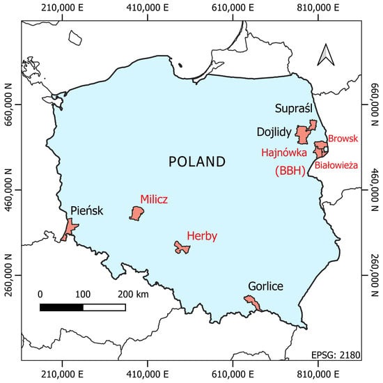
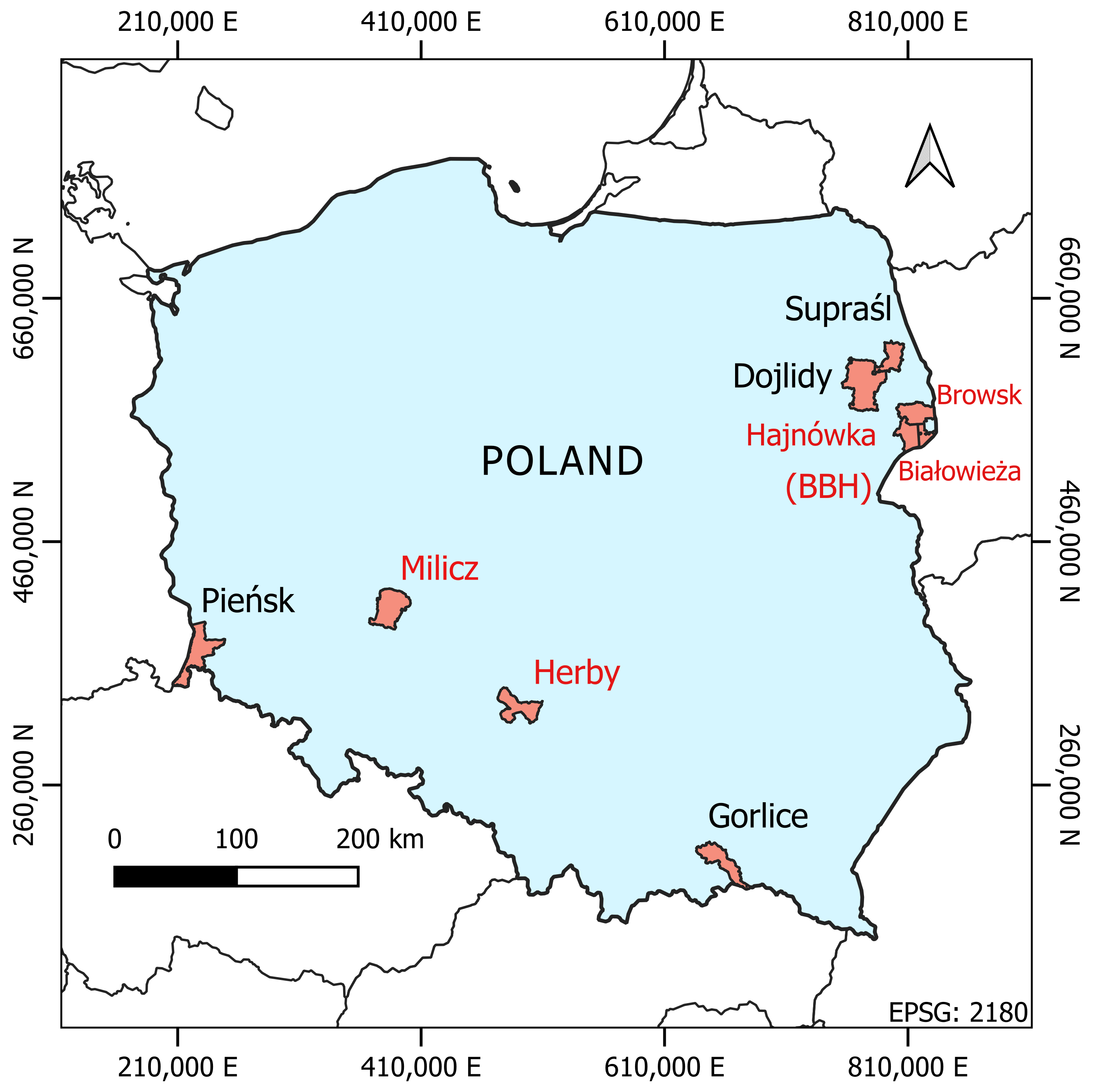
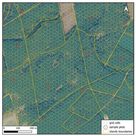
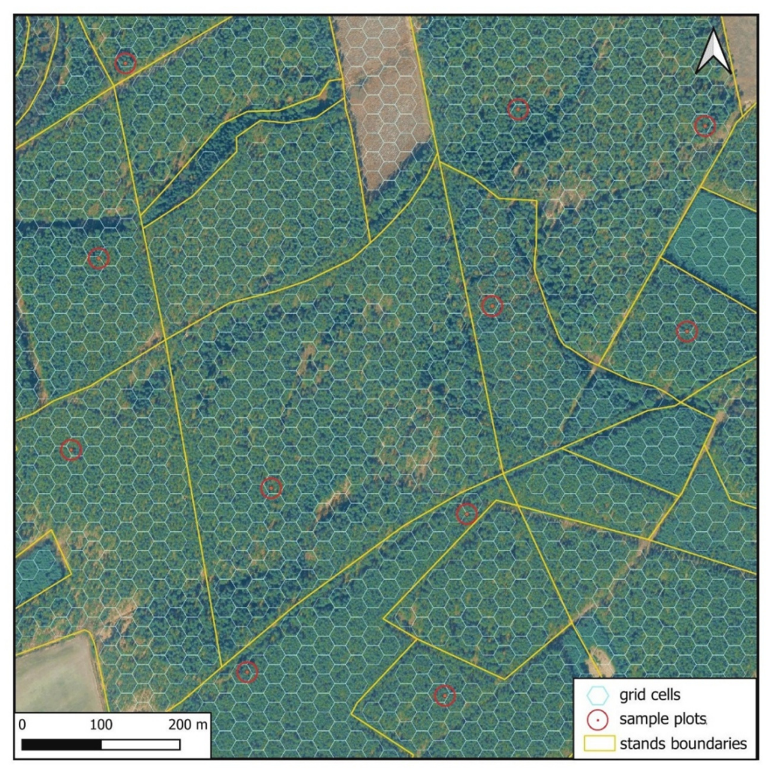
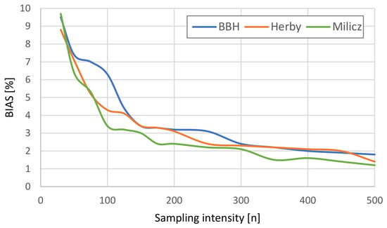
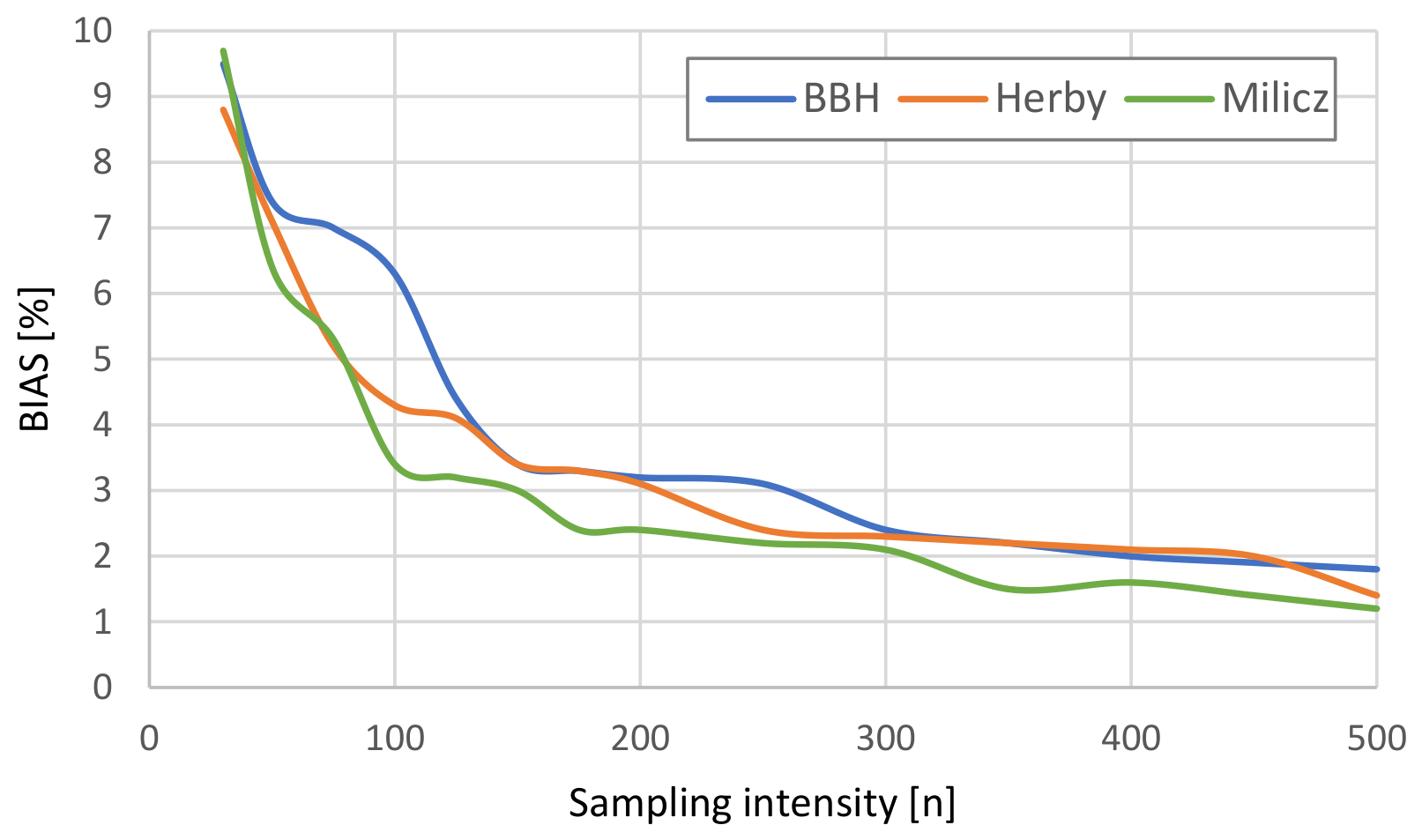
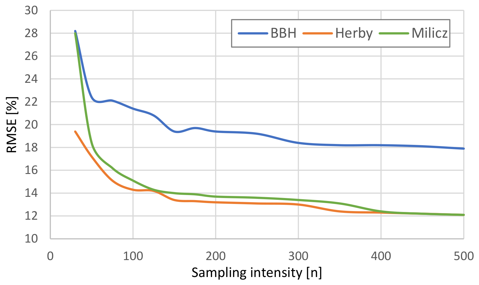
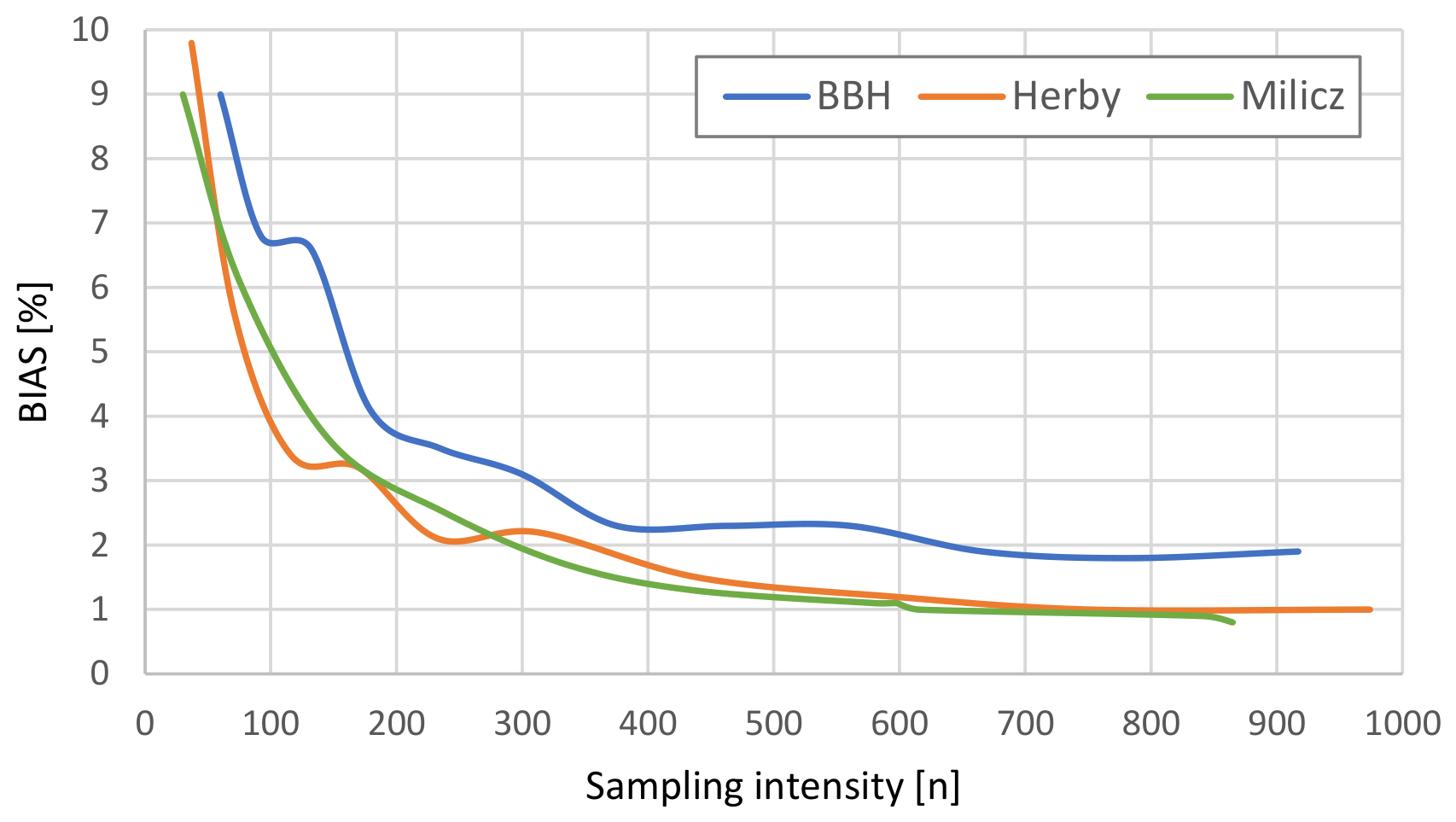
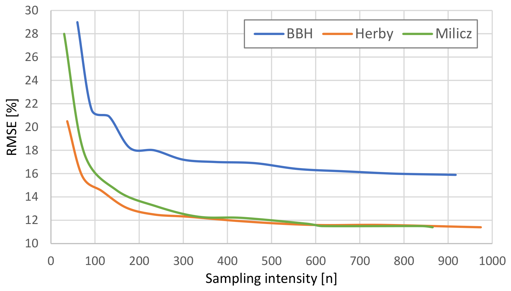
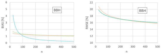
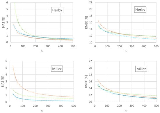
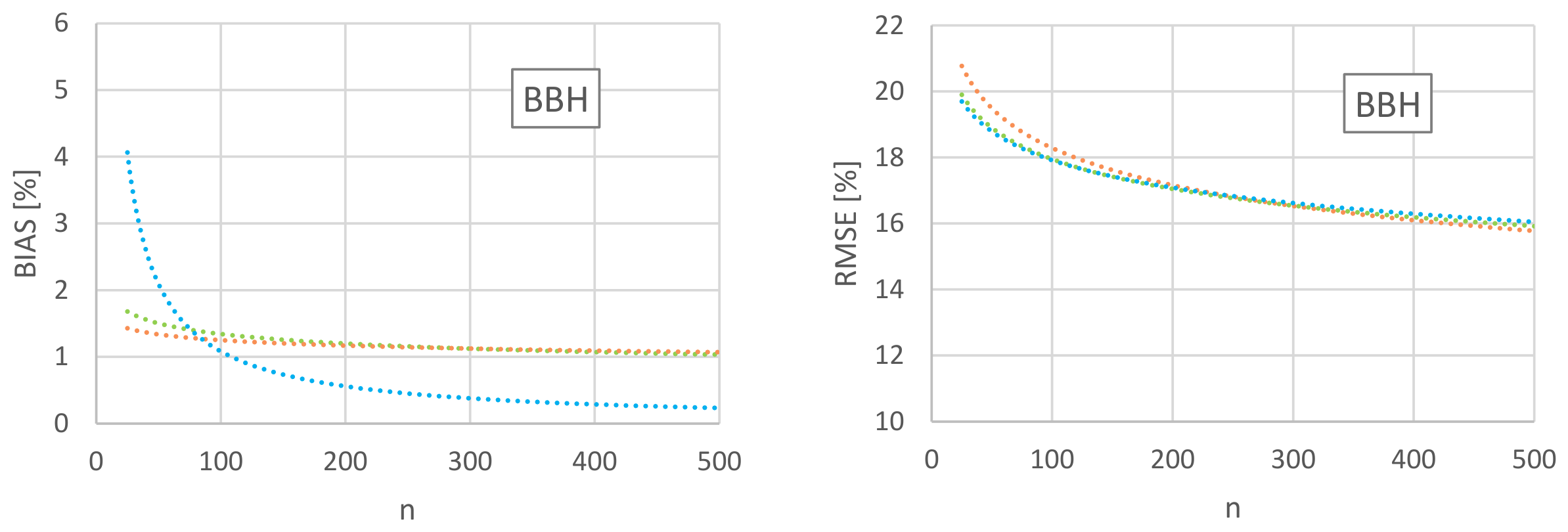
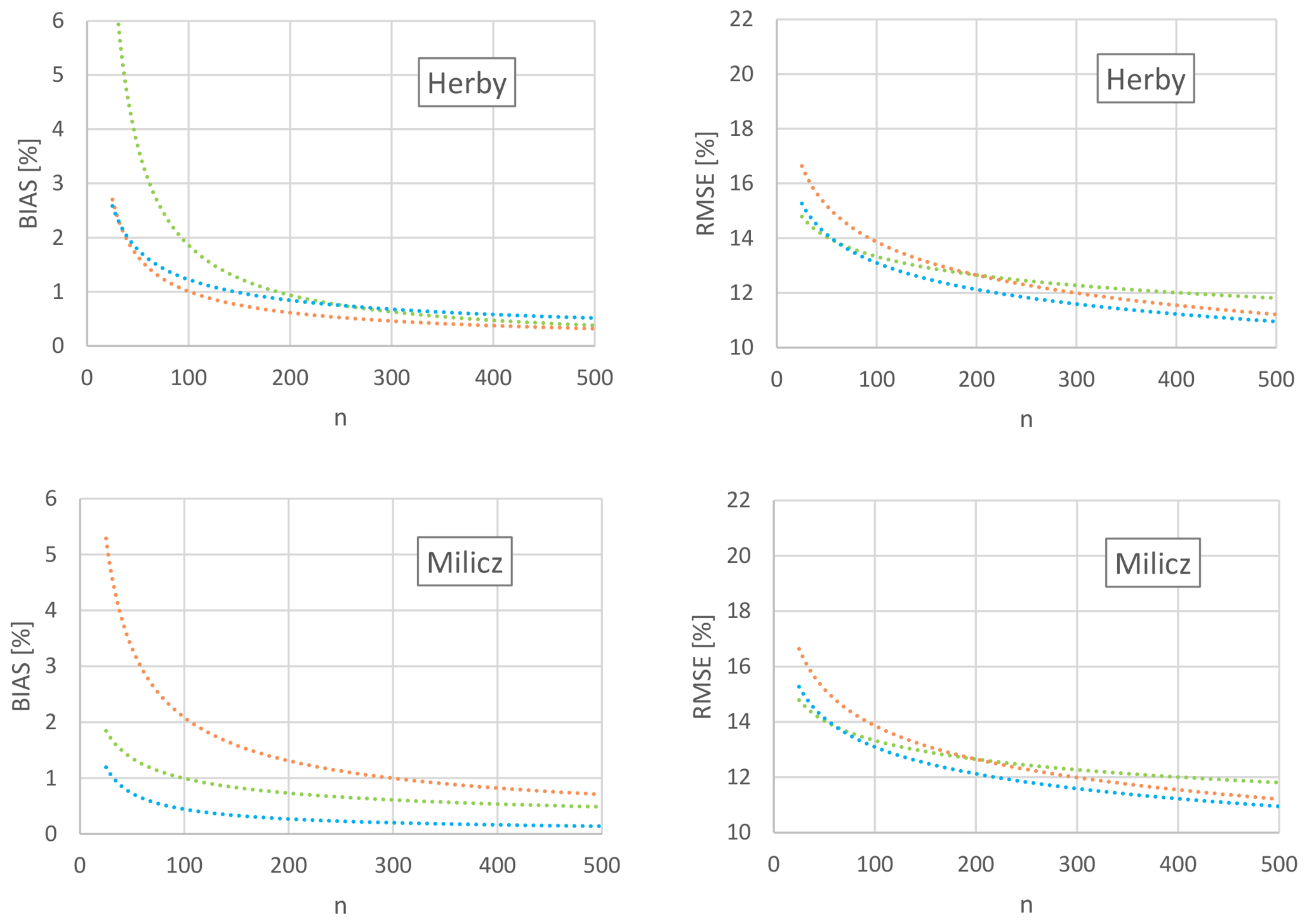
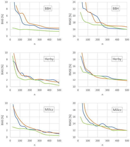
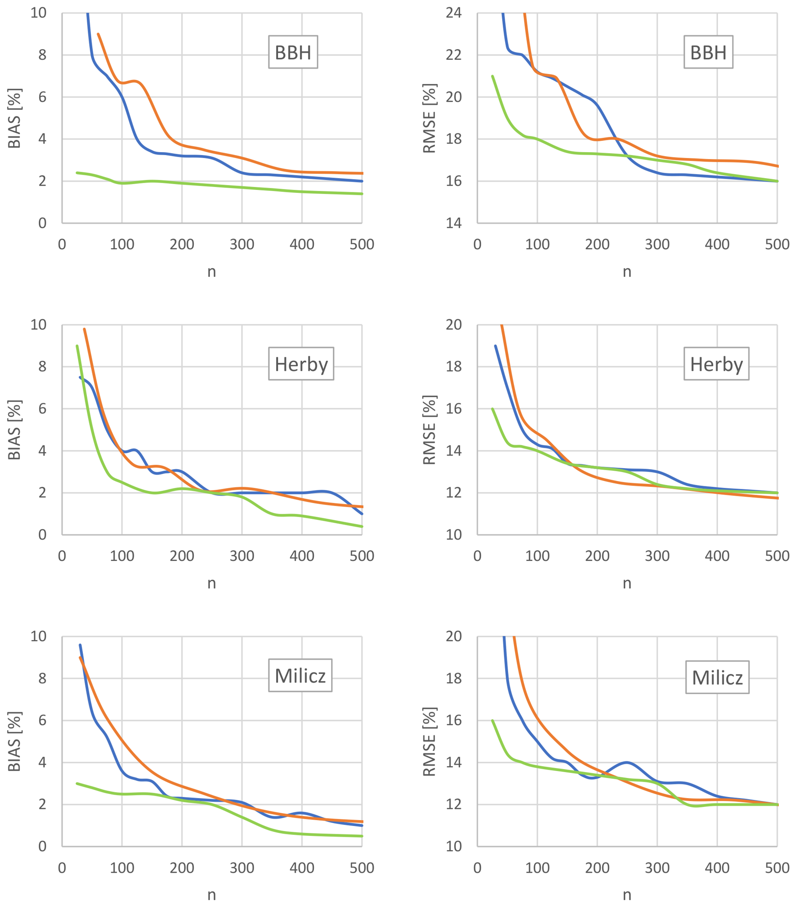
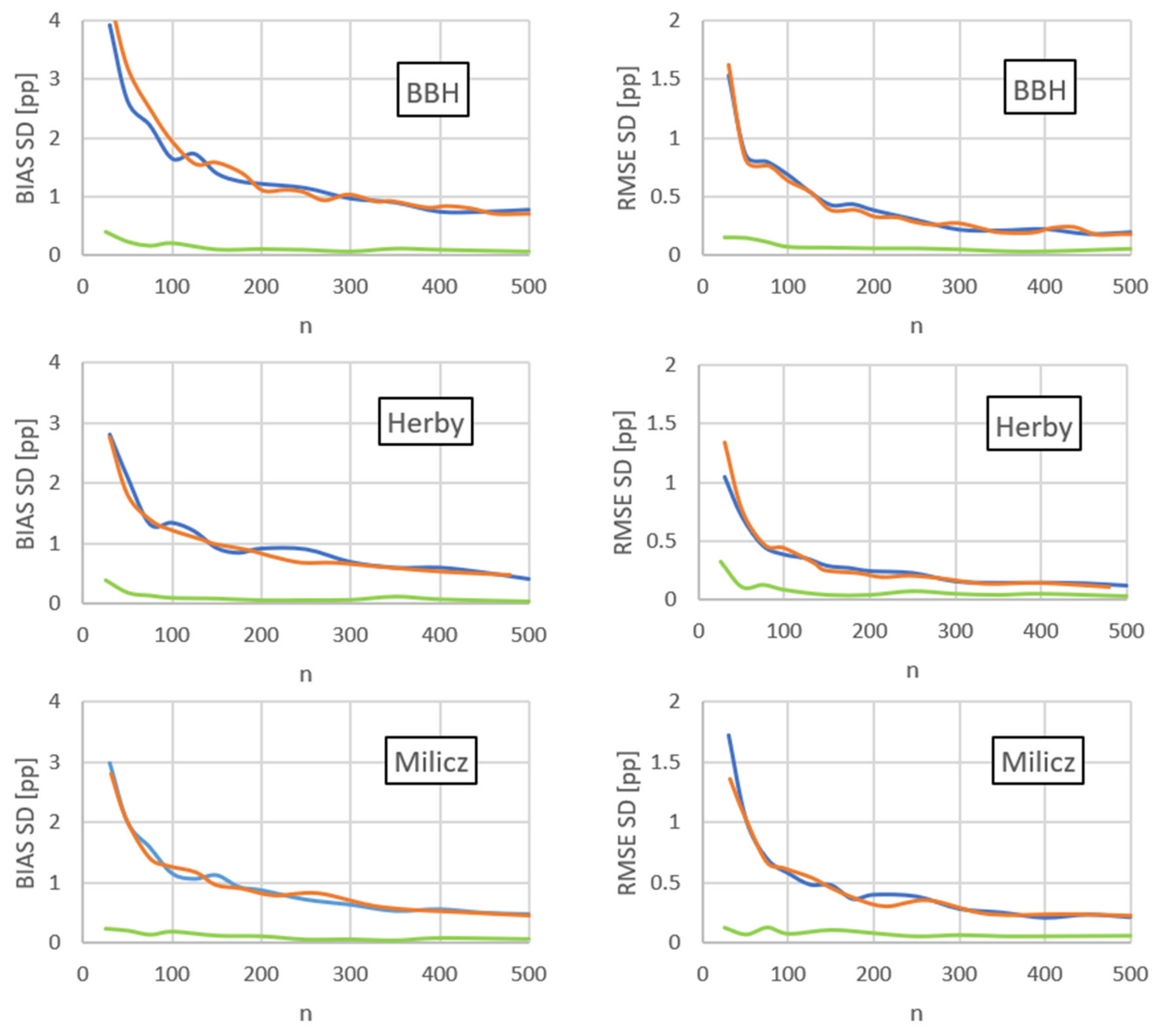

Disclaimer/Publisher’s Note: The statements, opinions and data contained in all publications are solely those of the individual author(s) and contributor(s) and not of MDPI and/or the editor(s). MDPI and/or the editor(s) disclaim responsibility for any injury to people or property resulting from any ideas, methods, instructions or products referred to in the content. |
© 2026 by the authors. Licensee MDPI, Basel, Switzerland. This article is an open access article distributed under the terms and conditions of the Creative Commons Attribution (CC BY) license.