


Highlights
- A task-oriented architecture (MFM-TransUNet) is proposed for surface water extraction.
- HPSM module captures local sequence context with linear complexity, suppressing background noise.
- EFA module integrates Sobel edge priors to significantly improve boundary extraction.
- Achieves a favorable trade-off between segmentation accuracy and computational cost.
- Extensive cross-dataset evaluations demonstrate the model’s robustness and generalization.
Abstract
Accurate extraction of surface water is of great significance for water resource management, ecological conservation, and flood disaster monitoring. However, water bodies in high-resolution remote sensing imagery are often obscured by building shadows, vegetation, complex backgrounds, or spectral confusion. Consequently, traditional semantic segmentation methods frequently struggle with global feature modeling and the preservation of boundary details. To address these challenges, this paper proposes MFM-TransUNet, a remote sensing water extraction network based on multi-scale feature modeling. The network employs an encoder–feature modeling–decoder architecture. A Ghost-SE encoder is utilized to extract multi-scale hierarchical features, while a High-Performance Sequence Modeling Module (HPSM) is introduced to aggregate local contextual information from high-level features through depthwise 1D convolutions, with a feed-forward network enhancing nonlinear feature representations along the channel dimension. During the decoding phase, a learnable weight-fusion strategy is applied to balance the contributions of features from different levels, and an Edge-enhanced Feature Attention (EFA) is incorporated to strengthen boundary-related information within the decoded features. The proposed method was evaluated in terms of segmentation accuracy, module ablation, and cross-dataset performance. Experiments on the GID dataset demonstrate that MFM-TransUNet achieves an Overall Accuracy (OA) of 96.27%, a Mean Intersection over Union (Mean IoU) of 89.24%, an F1-Score of 94.20%, and a Boundary IoU of 63.52%, showing competitive performance compared with several mainstream baseline models. Ablation studies evaluate the contributions of the key modules, while experiments on the LJ-Water and Water-CD datasets assess the model’s performance across different datasets. These results suggest that MFM-TransUNet achieves a favorable trade-off between segmentation accuracy, boundary-related performance, and computational cost, providing a potential approach for surface water extraction in complex remote sensing scenarios.
1. Introduction
Surface water bodies, including rivers, lakes, ponds, reservoirs, and wetlands, are crucial components of global ecosystems and fundamental to human development [1]. Surface water information serves as a core data source for water resource surveys [2], flood risk assessment [3], wetland ecological protection [4], and land use planning [5]. Therefore, efficient and accurate surface water monitoring techniques are of great strategic significance for sustainable water management.
The rapid advancement of remote sensing technology has provided a novel paradigm for large-scale surface water monitoring [6,7,8]. In recent years, many researchers have focused on surface water body extraction from satellite remote sensing imagery. By applying deep learning to remote sensing image analysis, water body extraction can be achieved with high precision and efficiency, offering powerful technical support for hydrological and ecological studies. Compared with traditional field surveys, satellite remote sensing offers broad coverage and periodic observation capabilities. In particular, the open accessibility of data from domestic Gaofen (GF) satellites, Landsat, and Sentinel missions provides abundant data sources for surface water body extraction research.
Early studies primarily relied on spectral index-based methods, such as the Normalized Difference Water Index (NDWI) [9], and threshold segmentation approaches [10]. However, these traditional methods are susceptible to interference from shadows, turbid waters, mountain occlusion, and high-reflectance urban surfaces, resulting in unstable classification accuracy under complex environmental conditions.
Driven by deep learning technology, models such as U-Net and DeepLabv3+ have significantly improved the accuracy of semantic segmentation of remote sensing imagery [11,12,13]. Compared with traditional machine learning methods, deep learning is capable of automatically learning features from a large number of samples, thereby better adapting to complex scenarios. Convolutional neural networks (CNNs) have become widely used deep-learning architectures because local connectivity and weight sharing can reduce the number of parameters relative to fully connected operations through local connections and weight sharing, whilst utilising convolutional operations to achieve hierarchical feature extraction [14,15]. Building on this, fully convolutional networks (FCNs) eliminate fully connected layers whilst retaining spatial information, and achieve pixel-level predictions through upsampling, thereby providing a crucial foundation for semantic segmentation [16]. Existing segmentation networks primarily fall into two categories: encoder-decoder and feature fusion. The former, represented by U-Net, SegNet [17], RefineNet [18] and LS3EU-Net++ [19], uses an encoder to extract high-level semantic features, which are then progressively restored as spatial information by the decoder; the latter, represented by the DeepLab series [20,21] and PSPNet [22], enhances global contextual representation through multi-scale feature fusion. Research has shown that segmentation performance is closely related to feature extraction capability [23]. Networks such as LeNet [24], AlexNet [25], GoogLeNet [26], VGGNet [27], ResNet [28] and DenseNet [29] have continuously improved feature representation capabilities and model performance through methods such as deepening the network, residual connections and dense connections. In recent years, deep learning has become a key technical approach for water body extraction in remote sensing, and methods based on U-Net and its modified variants have been widely applied to the segmentation of water bodies in medium- and high-resolution remote sensing imagery [30,31,32,33,34]. However, standard convolutional operations aggregate information primarily within local receptive fields. Although deeper networks can expand the effective receptive field, modeling long-range interactions remains challenging; consequently, the ability to recognise water bodies in complex backgrounds requires further improvement.
To address issues such as wide variations in the scale of water bodies and blurred boundaries in high-resolution remote sensing imagery, researchers have proposed a variety of improved methods. For example, the Multi-scale Water Body Extraction Convolutional Neural Network (MWEN) enhances the integrity of water body boundaries by fusing multi-scale features, and outperforms FCN, U-Net and DeepLab V3+ on GF-1 imagery [35]. To address differences in data distribution across different sensors, the Dense Local Feature Compression Network (DLFC) achieves cross-sensor water body extraction by adaptively learning the distribution of image features [36]. For example, Wieland et al. investigated the semantic segmentation of water bodies using ultra-high-resolution satellite and aerial imagery, and systematically evaluated model performance across various sensors and platforms, highlighting the importance of model generalization capability [37]. To address the issue of shadows cast by high-rise buildings in urban areas being mistakenly classified as water bodies, the attention-based improved U-Net and the SPFDNet, which combines spatial partitioning with feature decoupling, effectively reduce false positives by enhancing water body boundary features and suppressing background noise [38,39]. Furthermore, Amin et al. (2024) noted that heterogeneous landscapes in complex mountainous terrain pose significant challenges for land-cover classification [40]; meanwhile, Shastry et al. confirmed that cloud cover and dense vegetation can severely compromise the accuracy of remote sensing-based flood mapping [41]. Synthesizing these findings, this paper defines “complex scenarios” specifically as heterogeneous aquatic environments characterized by the presence of mountain shadows, dense vegetation, narrow or elongated tributaries, and irregular natural shorelines. Beyond water bodies, semantic segmentation techniques have also advanced in other specific remote sensing extraction tasks. For instance, Gong et al. proposed HSRoadNet utilizing an improved SE module for road extraction [42], and Zhou et al. developed RFTransUNet based on cross Vision Transformers for building extraction [43].
With the advancement of Transformers in computer vision tasks, TransUNet has demonstrated how global self-attention can be integrated into an encoder–decoder architecture for semantic segmentation [44]. This model integrates the global dependency modelling capabilities of Transformers with the encoder-decoder structure of U-Net, preserving multi-scale spatial features whilst capturing long-range contextual information [45,46]. Addressing the challenge posed by similarities in water depth characteristics, Richardson et al. utilized Sentinel-2 imagery to demonstrate that spatial context information is indispensable for distinguishing between optically shallow and deep waters [47]. However, due to factors such as variations in the scale of remote sensing imagery, the complexity of land cover types, and the diverse morphology of water bodies, the baseline TransUNet still exhibits certain limitations in the recognition of small-scale water bodies, the restoration of edge details, and adaptation to complex scenes. It is therefore necessary to further enhance the modelling capabilities for multi-scale feature representation and boundary information in order to improve the performance of water body extraction in complex remote sensing scenes.
To address the aforementioned shortcomings, researchers have conducted extensive studies focusing on feature representation enhancement and multi-scale information fusion. For example, MEF-TransUNet introduces a multi-scale edge-guided attention module (MEGA) and a high-low frequency decomposition fusion module (HLFD), optimised to address the issues of fragmented edges and false detections in small water bodies within high-resolution imagery; by enhancing edge information extraction and multi-frequency feature fusion, it improves the completeness and recognition accuracy of complex water body targets [48]. Furthermore, a dual-branch collaborative mechanism can effectively harness the complementary strengths of CNNs and Transformers. IC-TransUNet constructs a dual-branch structure comprising a CNN and a Transformer, enabling the collaborative learning of local texture and global semantic information, and achieving better segmentation results in scenarios characterised by class imbalance and easily confused small objects [49]. ViTenc-UNet, on the other hand, integrates a Vision Transformer encoder into the U-Net framework, effectively alleviating the shortcomings of traditional CNNs in modelling long-range spatial dependencies and achieving high-precision identification of water bodies in lakes on the Qinghai–Tibet Plateau [50]. These studies demonstrate that the performance improvements of TransUNet do not simply rely on the stacking of modules, but rather achieve deep coupling between the spectral information of water bodies and their spatial morphological features through targeted attention mechanisms and feature fusion strategies [51,52].
To address these challenges, researchers have explored various approaches, including frequency-domain interaction, multimodal fusion, and sequence modeling. AFENet [53] and SiMultiF [54] utilize frequency-domain modulation and cross-attention to facilitate multidimensional feature interaction, thereby alleviating segmentation difficulties in complex scenes. Sequence modeling offers a novel perspective for capturing long-range dependencies [55,56,57,58]; for instance, HyMambaNet [59] and HWBENet [60] enhance accuracy through hybrid sequence modeling and hierarchical representation, respectively. State-space models and convolutional approaches provide alternative mechanisms for contextual modeling. Their ability to capture long-range dependencies depends on the specific architecture and configuration, whereas standard global self-attention explicitly models pairwise interactions among all tokens. Furthermore, EGA-Net [61] improves boundary localization through dual-gated aggregation, while Lodhi et al. [62] demonstrate the efficacy of adaptive fusion via macro-level weighted integration. In contrast, this paper focuses on micro-level feature fusion, dynamically adjusting the ratio of deep and shallow features within the decoder to directly incorporate pixel-level gradients, thereby achieving more precise spatial alignment.
While the aforementioned studies provide diverse pathways for water body extraction, they encounter significant challenges when applied to high-resolution imagery, such as the high computational cost of global attention and the potential loss of boundary information in deeper layers. To address these challenges, this paper proposes MFM-TransUNet, which combines hierarchical feature extraction, local sequence-context aggregation, learnable multi-scale fusion, and edge-aware feature modulation. Specifically, the High-Performance Sequence Modeling Module (HPSM) uses depthwise 1D convolution to aggregate local information along the serialized feature sequence. For a fixed feature dimension and convolutional configuration, this operation has computational complexity that scales linearly with the sequence length, unlike the quadratic sequence-length complexity of standard global self-attention. The Edge-enhanced Feature Attention (EFA) head combines channel attention, spatial attention, and a Sobel-derived gradient prior to modulate decoded features. In addition, the Ghost-SE encoder and learnable weighted-fusion decoder are designed to balance feature representation and computational cost. Under the reported evaluation settings, MFM-TransUNet achieves competitive segmentation and boundary-related performance with 41.50 million parameters and 14.90 GFLOPs [63,64]. The main contributions of this paper are as follows:
- A Ghost-HPSM hybrid feature encoding framework is constructed, which combines the multi-scale feature extraction of the Ghost-SE hierarchical encoder with the local sequence context aggregation of HPSM. The local information interaction of high-level features is supplemented by deep one-dimensional convolution and feedforward network, forming a feature encoding strategy for remote sensing water body extraction tasks.
- An Edge-enhanced Feature Attention (EFA) head is introduced to combine channel attention, spatial attention, and a Sobel-derived gradient prior. The gradient prior modulates the decoded features to support boundary-related representation, with its contribution evaluated through module ablation and boundary-sensitive metrics.
- A learnable weighted-fusion strategy is introduced in the multi-scale decoder to adaptively balance the contributions of features from different levels, enabling the integration of shallow spatial details and deeper semantic representations during water-body reconstruction.
- Systematic experiments are conducted using GID and two Sentinel-2 water-body datasets. Through comparative and ablation studies, the effectiveness of MFM-TransUNet is verified in terms of segmentation accuracy, model complexity, and generalization capability.
The remainder of this paper is organized as follows: Section 2 describes the proposed architecture and its key modules. Section 3 presents the experimental datasets, implementation details, and quantitative and qualitative results. Section 4 discusses the findings and limitations, while Section 5 concludes the paper and outlines future research directions.
2. Materials and Methods
This paper proposes MFM-TransUNet, a multi-scale feature modeling network designed for water body extraction from remote sensing imagery. The model aims to harmonize hierarchical feature extraction, local sequence context aggregation, multi-scale feature fusion, and the enhancement of boundary information. It employs an encoder–feature modeling–decoder architecture, integrating a Ghost-SE hierarchical encoder, an HPSM module, a learnable weighted fusion decoder, and an Edge-enhanced Feature Attention mechanism. Within this framework, the HPSM module aggregates contextual information across a limited sequence neighborhood via depthwise 1D convolutions and utilizes a feed-forward network to bolster the non-linear representational capacity of the features. The multi-scale decoder is responsible for integrating features from various hierarchical levels, while the EFA module serves to reinforce edge-related information within the decoded features.
2.1. Overall Architecture
As shown in Figure 1, the MFM-TransUNet consists of four main components: a shallow feature extraction module (Stem), a hierarchical Ghost-SE encoder, a lightweight sequence modelling module, and a multi-scale decoder with an edge-enhanced attention head. The model takes high-resolution remote sensing imagery as input and adopts a U-shaped symmetric architecture. The encoder performs progressive downsampling to extract multi-scale hierarchical features. The HPSM converts the high-level features from the end of the encoder into a sequence representation, which then undergoes a series of transformations-layer normalization, depthwise 1D convolution, a feed-forward network, and residual connections. The depthwise 1D convolution aggregates local neighborhood information along the sequence dimension, with multiple stacked layers gradually expanding the theoretical receptive field; the feed-forward network further enhances non-linear representation within the channel dimension. This module serves to supplement the high-level features with local contextual information, without directly employing global self-attention or selective state-space operations. The decoder fuses features from different levels using learnable weights, and an EFA module subsequently enhances the decoded features across channel, spatial, and edge dimensions, ultimately producing pixel-level water body predictions. This architecture is designed to harmonize various functions, including local feature extraction, sequential context aggregation, multi-scale information fusion, and boundary refinement.
Figure 1.
Overall architecture of the proposed MFM-TransUNet framework.
Let the input remote sensing image be , where H and W are the height and width of the image, respectively, and C is the number of input bands. The model feeds the image into the Ghost-SE encoder to perform multi-scale hierarchical feature extraction, outputting a multi-scale feature sequence. The forward propagation process can be formally represented as
where denotes the Ghost-SE hierarchical encoder, and , , , and represent the encoded features at different network levels. The high-level feature representation is processed by HPSM as to aggregate local sequence context. The multi-scale decoder then progressively restores spatial resolution, fuses features from different levels, and generates the final prediction:
where Y denotes the model output, which provides pixel-wise predictions for the water and non-water classes. By combining hierarchical feature extraction, local sequence-context aggregation through HPSM, and cross-scale feature fusion in the decoder, MFM-TransUNet is designed to improve water-region continuity while preserving boundary details.
2.2. Ghost-SE Lightweight Feature Encoder
High-resolution remote sensing imagery is characterised by large spatial dimensions and complex land cover types, placing significant strain on traditional convolutional encoders in terms of both the number of parameters and computational overhead. As shown in Figure 2, this paper proposes the Ghost-SE hierarchical encoder, which reduces feature redundancy in convolutional operations through the Ghost feature generation mechanism and introduces an SE channel attention mechanism to enhance the response of feature channels related to water bodies. The encoder as a whole comprises a shallow feature extraction module and three stacked sets of Ghost-SE hierarchical bottlenecks.
Figure 2.
Diagram of Ghost-SE Bottleneck.
2.2.1. Shallow Feature Extraction Module
To obtain the initial shallow-layer spatial features of remote sensing imagery, this paper designs a shallow-layer feature extraction module (Stem module) to perform basic feature extraction. This module comprises a 7 × 7 convolution, batch normalisation, the ReLU activation function, and max-pooling.
For an input remote sensing image X, the stem module first extracts shallow spatial features using a convolution, denoted by . Batch normalization and a nonlinear activation function are then applied to the convolutional features to improve feature conditioning.
where denotes the batch normalisation operation, and is a non-linear activation function.
Finally, a max-pooling operation is applied to reduce the spatial dimensions of the feature map and expand the model’s receptive field:
This module effectively reduces the computational load on subsequent network layers whilst preserving the core spatial structural information of the image, thereby improving the model’s overall computational efficiency.
2.2.2. Ghost Feature Generation Mechanism
Traditional convolutional networks generate complete feature maps by applying a large number of convolutional kernels. Existing research indicates that the features extracted by deep neural networks contain a significant amount of redundant information, meaning it is not necessary to generate all features through complete convolutional operations. The Ghost module generates core eigenfeatures using a small number of standard convolutions, and then generates redundant, similar features via low-cost linear transformations, thereby completing the full feature mapping with fewer parameters. First, core intrinsic features are generated via standard convolution:
Next, Ghost redundant features are generated via lightweight linear transformations:
where denotes low-cost linear transformation operations such as deep convolution.
Finally, the eigenfeatures and redundant features are concatenated to obtain the complete output features of the Ghost module:
2.2.3. Ghost-SE Bottleneck Module
To further enhance the response of channels related to water-body features, this paper introduces an SE channel attention mechanism into the Ghost bottleneck structure to construct the Ghost-SE bottleneck module. Let the input to the bottleneck module be , and its forward computation process is as follows:
where and denote the two Ghost feature-generation stages, denotes depthwise convolution, and denotes the squeeze-and-excitation channel-attention operation. The skip feature provides a residual pathway that preserves input information when the dimensions are compatible.
2.2.4. SE Channel Attention Mechanism
Remote sensing imagery features a complex background, with interfering elements such as vegetation, buildings, and shadows intermingling with water bodies; there are significant differences in the contribution of features from different channels to the segmentation of water bodies. This paper introduces an SE-channel attention module to adaptively calibrate the feature weights of each channel.
Let the input feature map be . First, global average pooling is applied to aggregate global spatial information across all channels, yielding the channel statistical features:
Subsequently, a two-stage fully connected layer is used to learn the channel weight mapping relationships, generating adaptive channel weight coefficients:
In the formula, and represent the learnable weights of convolutions, which are used to normalize the channel weights to the range of .
Finally, the original features are weighted and corrected using the channel weights to obtain the optimised features:
Through this adaptive calibration mechanism, the network can autonomously enhance the feature channel responses corresponding to aquatic targets, whilst attenuating background interference features such as vegetation, buildings and shadows, thereby improving the model’s ability to focus on the features of aquatic targets.
2.3. High-Performance Sequence Modeling Module (HPSM)
As shown in Figure 3, the high-level semantic features output at the end of an encoder contain rich semantic information about targets; however, the scope over which local convolution operations can aggregate spatial context is constrained by the kernel size and the depth of the network. To further enhance the contextual representation of these high-level features while keeping computational overhead under control, this paper employs an Efficient Sequential Context Modeling module. HPSM is designed to augment the high-level feature representations from the encoder using convolutional local information interactions. The module consists of layer normalization, depthwise 1D convolution, a feed-forward network, and residual connections; here, the depthwise 1D convolution extracts local context along the sequence dimension, while the feed-forward network facilitates non-linear feature transformations across the channel dimension. Unlike explicit global self-attention or selective state-space modeling, the information propagation range in HPSM is determined by a combination of the kernel size, the dilation rate, and the number of stacked layers.
Figure 3.
Diagram of HPSM block.
2.3.1. Feature Serialization and Positional Encoding
The high-level semantic features extracted by the Ghost-SE encoder are denoted as , where and represent the spatial dimensions of the feature map, and represents the number of feature channels; these features contain rich multi-scale spatial and semantic information.
To prepare the high-level feature map for sequence processing, a convolution first projects the channel dimension to a common embedding dimension:
Subsequently, the two-dimensional spatial feature map is flattened into a one-dimensional feature sequence to achieve spatial feature serialisation:
where N is the total sequence length, and each token corresponds to a high-dimensional semantic feature at a spatial position.
The process of flattening two-dimensional features results in the loss of original spatial position information, leading to a lack of spatial constraints in sequence modelling. To address this, this paper introduces a learnable position encoding to supplement the sequence tokens with explicit spatial position information:
In the formula, P represents the learnable position embedding matrix. Position encoding enables HPSM to integrate semantic features with spatial position features, thereby enhancing the accuracy of global modelling.
2.3.2. HPSM: Local Sequence Context Modeling Unit
The HPSM consists of layer normalisation, 1D deep convolution, a feedforward network, and residual connections. Let the input sequence feature of the lth HPSM unit be . First, layer normalisation is applied to stabilise the feature distribution and mitigate the problem of gradient vanishing in deep networks:
Subsequently, a deep one-dimensional convolution is employed to aggregate local feature information from adjacent positions along the sequence dimension. This convolution performs local operations independently across each feature channel, enabling the extraction of contextual variations within the sequence’s neighborhood with a relatively low parameter overhead. Through the stacking of multiple layers, the propagation range of local information expands in tandem with the growth of the theoretical receptive field:
Compared with two-dimensional convolution, one-dimensional deep convolution acts directly on the spatial features of a sequence, enabling it to accurately capture the patterns of contextual changes across contiguous spatial regions, whilst reducing the computational complexity from to .
A feedforward network is introduced to enhance the non-linear representation of features and uncover complex semantic relationships:
where and are the dimension-up and dimension-down mapping matrices, respectively.
Finally, residual connections are employed to optimise feature superposition and prevent gradient vanishing in deep networks:
Following iterative processing through stacked HPSM blocks, the resulting sequence features incorporate local contextual information propagated across neighboring spatial tokens, with the effective receptive field increasing according to the convolutional configuration and network depth:
2.3.3. Feature Reconstruction and Channel Adjustment
To achieve multi-scale feature fusion with the decoder, the one-dimensional sequence features output by the HPSM must be reconstructed into a two-dimensional spatial feature map, thereby restoring spatial structural information:
The reconstructed feature maps retain the spatial structural information extracted by the encoder and incorporate local sequential context aggregated by the HPSM via deep 1D convolutions. The former provides a spatial structural foundation for subsequent decoding, while the latter supplements information interaction among high-level features within local sequential neighborhoods. Together, these serve as inputs to the multi-scale decoder, providing the necessary feature support for subsequent feature fusion and the reconstruction of water-covered regions.
To align with the decoder’s channel dimension, the reconstructed features HPSM undergo channel adjustment via a 3 × 3 convolution and batch normalisation:
The adjusted feature serves as the decoder’s initial input.
2.4. Multi-Scale Decoder with Learnable Weight Fusion
This paper constructs a multi-scale decoder based on the U-Net architecture, progressively restoring the spatial resolution of feature maps and fusing multi-scale encoded features to achieve fine-grained segmentation. The decoder employs a method of progressive upsampling and cross-layer feature fusion to effectively combine high-level semantic information with low-level spatial details, thereby enhancing the model’s ability to represent water body boundaries, fine-scale water body structures, and local regions. The decoder comprises four levels of decoding units. For each level, bilinear interpolation is used to up-sample the input features, and the up-sampled high-level semantic features are fused with the shallow-level features from the corresponding layer of the encoder. Convolution and batch normalisation are then applied to further extract and optimise the fused features, enabling the network to adaptively adjust the contribution of features at different levels based on the training data.
2.4.1. Learnable Weight Fusion Module
Traditional U-Net decoders employ channel concatenation to fuse shallow and deep features; however, this approach treats the two feature streams equally and cannot adaptively control the contribution ratio of features from different levels. Whilst shallow features contain rich spatial details, they also contain a significant amount of background noise; deep-layer features are rich in semantic information but relatively lacking in spatial detail. If these are fused indiscriminately, it is easy to introduce noise interference.
To this end, this paper designs a learnable weight fusion module, which uses learnable parameters to adaptively adjust the contribution ratios of the two feature streams. Let the backbone features be denoted as , and the skip connection features as ; the forward computation of the fusion module is as follows:
In the equation, and represent 1 × 1 convolutional projections (which degenerate into identity mappings when the number of input channels equals the number of output channels), whilst and are learnable weight parameters, both initially set to 1. The learnable weights enable the network to adaptively determine, based on the training data, the relative contributions of shallow-layer spatial details and deep-layer semantic features, thereby avoiding interference from shallow-layer noise.
2.4.2. Multi-Level Decoding Process
Deep-level features possess strong semantic representation capabilities, whilst shallow-level features retain richer spatial detail information. The decoder restores the features level by level, starting from the highest-level semantic features. In the first decoding stage, the input feature with spatial resolution is upsampled by a factor of 2 to and then fused with the output from the third stage of the encoder, whose channels have been adjusted via a convolution. The fused feature is processed by a convolution, batch normalisation and ReLU activation, yielding a feature with channels at . In the second decoding stage, this feature is further upsampled by a factor of 4 to and fused with the output from the second encoder stage. After a convolution with batch normalisation and ReLU, the channel dimension is reduced to C at . In the third decoding stage, the feature is upsampled by a factor of 4 to and fused with the output from the first encoder stage, whose channels have been adjusted via a convolution. A subsequent convolution with batch normalisation and ReLU reduces the channels to at . Finally, in the fourth decoding stage, the feature is upsampled by a factor of 2 to the original input resolution and passed through a convolution with batch normalisation and ReLU, yielding a high-resolution feature representation with channels. This feature map, which combines high spatial resolution with strong semantic representation, serves as the input to the subsequent edge-enhanced attention head.
2.5. Edge-Enhanced Feature Attention (EFA)
Water body boundaries in remote sensing imagery typically exhibit significant spatial uncertainty, particularly in areas such as shoreline transition zones, narrow river channels and small tributaries, where they are susceptible to the influence of complex background textures and mixed pixels, leading to inaccurate boundary localisation and discontinuities in local water body structures. To address these issues, this paper proposes the EFA head, which enhances decoded features across three complementary dimensions—channel, spatial and edge—as shown in Figure 4.
Figure 4.
Diagram of EFA block.
2.5.1. Channel Attention Branch
Let the EFA input features be denoted by F. The channel attention branch first aggregates spatial information across channels via global average pooling, and then generates channel weights through two layers of 1 × 1 convolutions followed by a Sigmoid activation function:
where and are learnable weights. The features enhanced by channel attention are
where ⊙ denotes element-wise multiplication. This branch is used to enhance the response of water-related channels and suppress interference from background channels.
2.5.2. Spatial Attention Branch
The spatial attention branch extracts spatial saliency via average pooling and max pooling along the channel dimension:
After concatenating the two into a 2-channel feature, a 5 × 5 convolution followed by a Sigmoid activation function generates the spatial weights:
The features enhanced by spatial attention are
This branch is used to focus on the target water body region and suppress interference from the background.
2.5.3. Sobel-Based Edge Prior
The EFA fuses channel attention, spatial attention, and a Sobel-based edge prior into a unified three-branch structure. Given an input feature map , a grayscale representation is first obtained by averaging across the channel dimension:
Two fixed Sobel kernels are then applied to to extract horizontal and vertical gradients:
The horizontal and vertical edge responses are computed as
where ∗ denotes the 2D convolution operation. The two directional responses are then combined into a single edge magnitude map:
with added for numerical stability. The final edge prior is obtained by applying a sigmoid activation:
This branch explicitly extracts geometric edge information of the shoreline using a fixed Sobel convolution, providing a geometric prior for boundary refinement. Although a fixed Sobel operator lacks the ability to adaptively learn features of water bodies at multiple scales, it offers highly sharp local gradient priors; this effectively compensates for the ambiguity of deep features at boundaries without incurring additional computational overhead.
2.5.4. Channel–Spatial–Edge Collaborative Fusion and Segmentation Head
The outputs of the channel attention branch and the spatial attention branch are added together, then multiplied by the output of the edge enhancement branch, thereby achieving Channel–Spatial–Edge collaborative feature enhancement:
The design logic for this fusion approach is as follows: and integrate semantic saliency across both channel and spatial dimensions, establishing a semantic feature foundation characterized by high redundancy. Meanwhile, E provides geometric edge priors; through element-wise multiplication, features in edge regions are enhanced while those in non-edge regions are suppressed, thereby enabling precise refinement of water body boundaries.
Finally, the enhanced features are fed into the segmentation head, which outputs the final pixel-level prediction results. The segmentation head comprises a depthwise separable 1D convolution, Dropout, and a 1 × 1 convolution:
where denotes a depthwise separable 2D convolution, and denotes the spatial Dropout operation. The final output Y corresponds to the class probability for each pixel belonging to either the water or non-water class.
2.6. Accuracy Evaluation
The extraction accuracy is evaluated using the Confusion Matrix (CM). Overall Accuracy (OA) is obtained by dividing the number of correctly classified samples by the total number of samples, and its formula is shown in (40). IoU is an evaluation criterion in the field of semantic segmentation, which calculates the ratio of the intersection over union of the set of pixels of the prediction results and the set of pixels of the true labels, with the formula shown in (41):
Precision (P) represents the ratio of correctly classified water body pixels in the image to the total number of water body pixels in the predicted image, which is defined as shown in (42); Recall (R) represents the ratio of correctly classified water body pixels to the total number of water body pixels in the real image, which is defined as shown in (43). F1-Score is a metric for evaluating the model based on the precision rate and recall rate, which is expressed as a weighted summed average of the two, which explains the degree of overlap between the true value and the predicted pixels, as defined in (44). The value of the F1-Score ranges from 0 to 1, with 1 representing the best output of the model, and 0 representing the worst output results of the model. The relevant equations are shown below:
Boundary IoU (BIoU) is defined as the ratio of the intersection to the union of the correctly predicted boundary pixel bands and the ground-truth boundary pixel bands, as expressed in Equation (45). BIoU is calculated by using morphological erosion to extract boundary bands of a specific width from the mask (in this study, the bandwidth scaling factor is set to 0.02); it is specifically designed to evaluate the accuracy of a model in localizing the boundaries of water-body shorelines and fine-scale structures. The value of BIoU ranges from 0 to 1, with 1 representing a perfect fit of the boundaries:
In this formula, N is the total number of images in the test set, while and represent the ground-truth and predicted masks for the i-th image, respectively; denotes the set of pixels within a boundary band—extracted based on the image’s diagonal length and a parameter —and represents the total number of pixels within that set.
2.7. Dataset
The remote sensing imagery utilized in this study is drawn from GID [65], which was constructed on the basis of GF-2 satellite data. The GF-2 satellite carries two panchromatic and multispectral sensors, with a spatial resolution of 1 m panchromatic and 4 m multispectral, and an imaging width of 45 km, and the specific parameters are shown in Table 1 below.
Table 1.
Parameters of GF-2 satellites.
The GID dataset consists of 150 pixel-level annotated GF-2 images, covering an area of over 50,000 square kilometers. Due to their broad geographical distribution, these images capture the diverse spatial distribution of land-cover features across various regions. Furthermore, the dataset includes images of the same or overlapping areas acquired at different times, resulting in a rich diversity of spectral responses and morphological structures. Regarding the surface water bodies investigated in this study, which encompass rivers, lakes, and ponds, the dataset features complex hydrological networks and aquatic environments, making it an excellent resource for model training. For this study, 50 images containing a significant proportion of water bodies were selected from the 150 available images to construct the training samples. These 50 source images were grouped based on their geographical location and acquisition time, and subsequently processed using a sliding-window cropping technique to generate the training, validation, and test sets.
The original remote sensing images are large, and due to the limitations of computer video memory, it is usually impossible to put the entire image into the model for training, otherwise there is a risk of memory overflow. In this study, we set the dimensions for both samples and labels to 512 × 512 pixels. We employed a sliding-window cropping approach, with an overlap rate of zero, ensuring that the image patches generated during the primary iteration do not overlap. To ensure full coverage of the image edges, padding-based cropping was applied to the final row, the final column, and the bottom-right corner, which inevitably introduced some localized overlap. To address this, we tracked the pixel coordinate range of each patch within the original image and performed post-processing to remove redundant, spatially overlapping patches—retaining only one instance of each—thereby ensuring that all image patches in the final dataset are spatially non-overlapping.
In this study, data enhancement is used to flip, rotate, and translate the original data, which increases the richness of the samples and effectively prevents the occurrence of overfitting in terms of model training. The data enhancement operations used in this study are vertical rotation, horizontal flip, and diagonal mirroring, and the specific effects are shown in Figure 5. It should be noted that data augmentation is applied only to the training set; the validation and test sets are not subjected to any augmentation.
Figure 5.
Data Enhancement Example.
Since the GID dataset contains annotations for five land-cover categories, the labeling process required masking all categories except for water bodies. The masked images were then filtered to exclude samples that did not contain any water bodies, resulting in a final dataset consisting of 700 images for training, 100 for validation, and 200 for testing. Figure 6 displays selected water samples and their corresponding labels, providing a visual representation of water distribution patterns and morphological variations within the imagery.
Figure 6.
Example of GF-2 image water sample.
3. Results
3.1. Experimental Setup
The programming language used in this paper is Python, and the deep learning framework is PyTorch. The specific experimental environment configuration parameters are shown in Table 2.
Table 2.
Experimental environment configuration.
The training process employs the Adam optimizer with an initial learning rate of , which is decayed using a cosine annealing strategy. The batch size is set to 4. A class-weighted cross-entropy loss function is used to mitigate the class imbalance between water and non-water samples. All comparative experiments were conducted using identical software, hardware, and training configurations to ensure a fair comparison. To guarantee the reliability of the results, each model was trained and evaluated five times, each with a different random seed; all metrics reported in this paper represent the average values across these five experimental runs.
3.2. Quantitative Analysis Results
To validate the effectiveness of the proposed MFM-TransUNet model in the task of water body extraction from remote sensing imagery, a selection of mainstream classical segmentation networks (UNet [11], SegNet [17]), Transformer-fused segmentation networks (TransUNet [44]), and recently developed improved segmentation networks (LS3EU-Net++ [19], AFENet [53], EGANet [61]) were chosen as comparison baselines for evaluation against the proposed algorithm. The experiments utilised five evaluation metrics: OA, IoU, Precision, Recall and F1-Score. Higher values for each metric indicate greater segmentation accuracy, completeness and robustness of the model.
As shown in Table 3, the proposed model achieves competitive overall performance, with an OA of 96.27%. This represents an improvement of 0.56, 1.83, 1.98, 2.06, 4.77, and 12.11 percentage points over AFENet, EGANet, LS3EU-Net++, UNet, SegNet, and TransUNet, respectively. Furthermore, the proposed model attains the highest values for Mean IoU (89.24%), Precision (94.61%), and F1-Score (94.20%), demonstrating exceptional pixel-level classification consistency and comprehensive segmentation performance within the test area.
Table 3.
Model accuracy comparison.
Compared to UNet, the proposed method yields improvements of 2.06% in OA, 4.44% in IoU, 5.09% in Precision, 2.63% in F1-Score, and 11.17% in Boundary IoU. While UNet achieves a relatively high Recall (94.21%), its Precision is comparatively lower (89.52%), suggesting a tendency to misclassify background pixels as targets, which leads to over-segmentation along object boundaries. In contrast, the proposed method enhances both Precision and regional overlap while maintaining a high Recall, indicating that the designed architecture effectively suppresses false detections and improves segmentation accuracy at object boundaries. Compared to SegNet, the proposed model shows improvements ranging from 1.26% to 17.67% across all metrics, highlighting its superior capability in feature extraction and fusion.
In this experiment, TransUNet exhibits relatively lower accuracy (OA 84.16%, IoU 62.68%). This may be attributed to the model’s increased complexity, as well as the sensitivity of global attention mechanisms to irrelevant contextual features within complex remote sensing scenes. Our proposed method outperforms TransUNet across all metrics, suggesting that for this segmentation task, our strategy, which focuses on local sequence modeling and feature fusion, is better suited to the characteristics of the dataset and more effective at mitigating interference from irrelevant background information.
Our method also demonstrates clear advantages over recent state-of-the-art models, such as LS3EU-Net++ and EGANet. Although LS3EU-Net++ achieves a high precision (93.59%), its recall is only 88.33%; the model tends toward conservative predictions, resulting in a significant number of missed detections (5.47% lower recall than our method). EGANet shows moderate overall performance (OA: 94.44%, IoU: 85.10%), whereas our method surpasses it by 1.83% in OA, 4.14% in IoU, 4.27% in precision, 2.46% in F1-score, and 12.63% in Boundary IoU.
Using the well-performing baseline model AFENet as a reference, the proposed model achieves improvements of 0.56%, 1.08%, 2.22%, and 0.62% in OA, IoU, Precision, and F1-Score, respectively. Although Recall shows a slight decline (1.13%), the overall performance demonstrates a consistent improvement. While AFENet achieves a high recall rate—aided by its feature enhancement module—it suffers from lower precision. In contrast, the proposed method effectively suppresses false detections at the cost of a minor reduction in recall, resulting in predictions that align more closely with the ground truth. Furthermore, in terms of Boundary IoU—a metric for assessing boundary-fitting accuracy—the proposed model attains a score of 63.52%, significantly outperforming AFENet (59.68%), UNet (52.35%), and EGANet (50.89%). This indicates that, while the gains in some conventional evaluation metrics are relatively modest, the overall performance improvement is robust. In particular, the incorporated EFA module effectively preserves boundary details at complex land–water interfaces, thereby enhancing the quality of boundary alignment in the segmentation results.
In summary, the proposed method achieves competitive results across key quantitative metrics. Compared to traditional CNNs, it offers better suppression of false detections and improved retention of edge details; compared to Transformer-based architectures, it avoids the introduction of background noise often caused by global attention mechanisms; and compared to state-of-the-art models, it maintains high precision while significantly mitigating issues related to missed detections and blurred boundaries. These results confirm that our method effectively balances false positives and false negatives, producing high-quality water segmentation results with exceptional boundary fidelity.
3.3. Qualitative Analysis Results
Figure 7 illustrates the results of water body extraction using a sample remote sensing image containing a large water body and a bridge structure spanning it. The figure shows Figure 7a the original remote sensing image, Figure 7b the ground truth, and Figure 7c–i the water body segmentation results from U-Net, SegNet, TransUNet, LS3EU-Net++, AFENet, EGANet and the model proposed in this paper, respectively. Judging from the visualisation results, U-Net is able to extract the main contours of the water body, but there is slight distortion at the edges surrounding the bridges, and the smoothness of local boundaries is insufficient. The overall performance is acceptable, but its ability to handle details of narrow, elongated obstacles such as bridges is limited. SegNet exhibits significant misclassification; there is a considerable amount of noise and voids within the water body, with some non-water areas along the shoreline incorrectly classified as water. The boundaries are severely jagged, and the overall accuracy is low. The segmentation results from TransUNet are severely incomplete, with large areas of the water body missed, and many water regions predicted as background; visually, this manifests as large swathes of water missing, indicating poor adaptability to this complex scene. LS3EU-Net++’s overall outline is close to the ground truth, but there are breaks in the bridge’s position, some shoreline details are lost, and there are instances of water body omissions. AFENet achieves a relatively good segmentation result with relatively complete boundaries, but there are still a few minor misclassifications near the bridge. While EGANet’s overall extraction performance is acceptable, there are noticeable breaks in the segmentation within bridge areas-preventing the preservation of water body connectivity, along with some misclassifications and noise in the vicinity of the bridges. The model presented in this paper is closest to the ground truth; it accurately distinguishes between bridges and water bodies, maintains the integrity of water connectivity at bridge locations, and exhibits a high degree of correspondence with the ground truth in terms of water body contours and shoreline edges. With minimal instances of voids and misclassification noise, this demonstrates that the model can effectively suppress segmentation errors caused by interfering features such as bridges and possesses stronger discrimination capabilities in the presence of complex feature interference.
Figure 7.
Comparison of water extraction results in main stream reach. In the image, the white areas represent water, while the black areas represent the background.
Figure 8 shows the results of water body extraction using different models on a remote sensing image of a downstream river section. Figure 8a shows the original remote sensing image; Figure 8b shows the ground truth; and Figure 8c–i show the water body segmentation results for U-Net, SegNet, TransUNet, LS3EU-Net++, AFENet, EGANet and the model proposed in this paper, respectively. U-Net is able to fully extract the main body of the river channel, but the details at the channel edges are coarse, with local edges appearing to contract inwards. SegNet exhibits severe edge jitter, with a large number of scattered false water patches on the outer side of the river channel, resulting in prominent false positives. TransUNet suffers from poor continuity at the river channel edges, with numerous edge gaps, and lacks the ability to reconstruct the boundaries of large-scale continuous water bodies. LS3EU-Net++ retains the overall morphology of the river channel well, but there is some loss of local detail at curved boundaries. AFENet and EGANet produce relatively high-quality boundaries, yet some minor distortions persist in certain sections of the shoreline. In contrast, the model proposed in this paper yields smooth and continuous river contours; its curved shorelines align almost perfectly with the ground truth, and there are few spurious patches. Quantitative evaluations using IoU and BoundaryIoU metrics demonstrate that the model’s boundary-aware module effectively refines water-body contours, enabling the generation of high-quality segmentation boundaries for large-scale, continuous river systems.
Figure 8.
Comparison of water body extraction results in the main stream reach. In the image, the white areas represent water, while the black areas represent the background.
Figure 9 shows the results of scenes with edge tributaries and complex shorelines. Figure 9a shows the original remote sensing image; Figure 9b shows the ground truth; and Figure 9c–i show the water body segmentation results for U-Net, SegNet, TransUNet, LS3EU-Net++, AFENet, EGANet and the model proposed in this paper, respectively. Such samples are typically characterised by complex structures, fragmented edges and strong background interference, and are well-suited to validating the performance of the various models in the task of detecting ‘fine-scale water bodies’. U-Net performs reasonably well in detecting the main river channel, but some narrow tributaries appear disconnected, and small water bodies are missed. SegNet loses a large number of small tributaries whilst introducing considerable background noise, and demonstrates weak performance in recognising small targets. TransUNet exhibits the most pronounced fragmentation of small water bodies, with many narrow watercourses being completely disconnected, which fully corresponds to its quantitatively low recall results. LS3EU-Net++ is able to retain some small watercourses, but disconnections still occur in certain extremely narrow water systems. AFENet exhibits better integrity of small water bodies than the aforementioned models, but a few minor tributaries still contain discontinuities. EGANet exhibits noticeable fragmentation and omissions when extracting narrow bridges, though it performs better in maintaining the continuity of small tributaries. The model proposed in this paper maintains connectivity for the majority of narrow and small watercourses, with fewer discontinuities; the integrity of small water bodies is significantly superior to that of the comparison algorithms. This demonstrates that the multi-scale feature fusion mechanism of the proposed model is capable of fully capturing the characteristics of small water bodies with low occurrence rates, thereby reducing the omission of such features.
Figure 9.
Scenes with edge tributaries and complex shorelines. In the image, the white areas represent water, while the black areas represent the background.
Across three representative scenarios, TransUNet exhibits varying degrees of missed detections, while SegNet consistently suffers from excessive noise and jagged boundaries. Although U-Net, LS3EU-Net++, AFENet, and EGANet are capable of extracting the main water bodies, they each have specific limitations, such as vulnerability to interference from bridges, difficulty in capturing narrow water channels, or challenges in preserving precise boundary details. In contrast, the model proposed in this paper performs effectively across scenarios involving bridge interference, broad main water channels, and narrow tributaries. It not only maintains the integrity of the primary water bodies while suppressing spurious noise, but also preserves complex boundaries and the details of narrow, elongated water features. The visualized segmentation masks are the closest to the ground truth, demonstrating that the proposed network achieves a balance between maintaining the integrity of large-scale water bodies and accurately extracting details for small-scale features and complex boundaries in water segmentation tasks.
4. Discussion and Analysis
4.1. Complexity Analysis
To evaluate the complexity and computational efficiency of the proposed model, we use the number of parameters, floating-point operations (FLOPs), weight storage requirements (in FP32/FP16 format), and model file size as evaluation metrics. We compare our model against TransUNet, U-Net, AFENet, SegNet, LS3EU-Net++, and EGA-Net; the results are presented in Table 4. Here, the number of parameters–measured in millions (M)–indicates the scale of the model, while FLOPs–measured in billions (G) of floating-point operations–represent the theoretical computational cost required for a single forward pass.
Table 4.
Complexity analysis results.
As shown in Table 4, the proposed model has a parameter count of 41.50 M, which is significantly lower than that of TransUNet (115.20 M), SegNet (167.80 M), and EGANet (103.84 M), representing reductions of approximately 63.97%, 75.26%, and 60.02%, respectively. In terms of computational overhead, the proposed model requires only 14.90 G FLOPs, marking a reduction of approximately 90.90%, 93.40%, and 90.72% compared to TransUNet (163.67 G), U-Net (225.84 G), and SegNet (160.68 G), respectively. It also achieves a reduction of approximately 41.77% in computational cost compared to AFENet (25.59 G). This demonstrates that the proposed model maintains a compact parameter scale while substantially lowering the theoretical computational cost of forward propagation.
Compared to TransUNet, the proposed model offers the dual advantages of a significantly reduced model size and lower computational requirements, alongside improved segmentation accuracy. As indicated by the experimental results in Table 3, the proposed model achieves notable gains in OA, Mean IoU, and F1-Score over TransUNet. Furthermore, in terms of complexity, it features a reduction of approximately 63.97% in parameters, 90.90% in FLOPs, and 63.97% in FP32 weight storage. This confirms that our approach does not sacrifice computational efficiency for higher accuracy; rather, it delivers superior segmentation results while simultaneously achieving a substantial reduction in both model size and computational demand.
When compared to both classic convolutional networks and lightweight networks, the proposed model also demonstrates an exceptionally low theoretical computational cost. Although U-Net has fewer parameters (24.90 M) than the proposed model, its FLOPs (225.84 G) are approximately 15.15 times higher. LS3EU-Net++ features the lowest number of parameters (4.38 M) and FLOPs (6.18 G), demonstrating an extremely lightweight design. In comparison, the proposed method has approximately 9.48 times the parameters and 2.41 times the FLOPs. This indicates that the proposed method achieves significantly higher overall segmentation accuracy and better completeness in target detection, at the cost of a modest increase in parameters and computational overhead.
Furthermore, regarding storage requirements, the proposed method’s weights occupy 158.33 MB in FP32 format and 79.16 MB in FP16 format; using FP16 half-precision effectively halves the static parameter storage requirements. It should be noted that model storage size is not equivalent to the VRAM (video memory) required during inference, as the latter also includes intermediate feature maps, temporary tensors, and other elements.
In summary, the experimental results demonstrate that the proposed method achieves an excellent balance between accuracy and computational cost.
4.2. Module Effectiveness Analysis
To verify the effectiveness of the key modules within MFM-TransUNet, five sets of ablation experiments were conducted. These involved replacing the Ghost convolution, as well as removing or replacing the HPSM module, the EFA head, and the learnable weight fusion module. The experimental results, presented in Table 5, show that the complete model achieves the best overall performance across metrics including OA, mean IoU, water-body IoU, mean Precision, mean F1, and BoundaryIoU, demonstrating that each module contributes positively to the final segmentation performance.
Table 5.
Comparison of ablation study results.
Replacing Ghost convolutions with standard 3 × 3 convolutions increases the model’s parameter count from 41.50 M to 85.34 M—a 105.6% rise—while simultaneously leading to a decline in key accuracy metrics. Specifically, OA drops from 96.27% to 95.53% (a decrease of 0.75 percentage points); mean IoU falls from 89.24% to 87.69% (down 1.55 percentage points); water-class IoU decreases from 83.04% to 80.90% (down 2.14 percentage points); water-class Precision drops from 91.87% to 86.04% (down 5.83 percentage points); mean Precision declines from 94.61% to 92.12% (down 2.50 percentage points); water-class F1-score falls from 90.73% to 89.44% (down 1.29 percentage points); mean F1-score decreases from 94.20% to 93.30% (down 0.90 percentage points); and Boundary IoU drops from 63.52% to 58.74% (down 4.78 percentage points). Although water-class Recall and mean Recall increase to 93.13% and 94.64%, respectively, the concurrent decline in Precision and F1-score indicates an increase in false positives. This demonstrates that by generating redundant features through inexpensive linear transformations, Ghost convolutions effectively reduce the encoder’s parameter count by approximately 51.3% while maintaining superior feature representation capability and overall segmentation accuracy.
Replacing HPSM with a standard Transformer-based global multi-head self-attention and MLP structure increases the model’s parameter count from 41.50 M to 98.13 M—a 136.4% increase—yet results in a decline in performance: OA drops from 96.27% to 95.99% (a decrease of 0.28 percentage points); mean IoU falls from 89.24% to 88.75% (down 0.49 percentage points); water-class IoU decreases from 83.04% to 82.44% (down 0.60 percentage points); water-class Precision drops from 91.87% to 88.31% (down 3.56 percentage points); mean Precision declines from 94.61% to 93.19% (down 1.43 percentage points); and Boundary IoU falls from 63.52% to 61.72% (down 1.80 percentage points). While the Transformer configuration improves water-class Recall and mean Recall to 92.54% and 94.71%, respectively, the declines in Precision, IoU, and Boundary IoU suggest that, although global self-attention enhances the recall of water bodies, its reliance on global pairwise interactions tends to introduce interference from background elements, such as shadows, buildings, and vegetation, thereby degrading spatial overlap and boundary quality for water regions. In contrast, HPSM employs depthwise separable 1D convolutions to propagate local context along the sequence dimension, replacing the quadratic complexity of self-attention with linear complexity. Compared to the Transformer-based configuration, the full model features 56.62 M fewer parameters while achieving improvements of 0.28, 0.49, 0.60, 0.28, and 1.80 percentage points in OA, mean IoU, water-class IoU, mean F1, and Boundary IoU, respectively, confirming that local sequence modeling is better aligned with the spatial continuity of water bodies. Removing the HPSM reduces the number of model parameters to 13.11 M-a 68.4% decrease compared to the full model, but results in a decline in performance: OA drops by 0.84 percentage points to 95.44%; mean IoU falls by 1.80 percentage points to 87.45%; water-body IoU decreases by 2.53 percentage points to 80.51%; water-body Precision drops by 5.83 percentage points to 86.04%; mean Precision declines by 2.56 percentage points to 92.06%; water-body F1-score falls by 1.53 percentage points to 89.20%; mean F1-score decreases by 1.04 percentage points to 93.16%; and Boundary IoU drops by 4.25 percentage points to 59.27%. Although water-body Recall and mean Recall increase to 92.60% and 94.39%, respectively, the declines in Precision, F1-score, IoU, and Boundary IoU indicate that the HPSM effectively enhances the integrity of water-body regions and improves boundary discrimination between water bodies and the background, all at an acceptable cost in terms of additional parameters.
Replacing the EFA with a 1 × 1 convolutional head results in a parameter count of 41.50 M, nearly identical to the 41.50 M of the full model-yet leads to a noticeable decline in accuracy. Specifically, the OA drops by 1.42 percentage points to 94.86%; mean IoU decreases by 3.15 percentage points to 86.09%; water-class IoU falls by 4.53 percentage points to 78.50%; water-class Precision drops by 7.86 percentage points to 84.01%; mean Precision declines by 3.62 percentage points to 91.00%; water-class F1-score decreases by 2.77 percentage points to 87.96%; mean F1-score drops by 1.85 percentage points to 92.35%; and Boundary IoU falls by 7.14 percentage points to 56.38%. These results demonstrate that the EFA-through the synergistic integration of channel attention, spatial attention, and Sobel edge priors-effectively enhances the accuracy of water-body boundary detection, proving particularly valuable for extracting narrow rivers and complex shoreline features. Replacing the learnable weight-based fusion with simple additive fusion leaves the parameter count virtually unchanged at 41.50 M, but results in a significant drop in accuracy. OA decreased to 94.70% (a drop of 1.57 percentage points); mean IoU fell to 85.80% (down 3.45 percentage points); water-class IoU dropped to 78.13% (down 4.90 percentage points); water-class Precision declined to 82.84% (down 9.03 percentage points); mean Precision decreased to 90.53% (down 4.10 percentage points); water-class F1 fell to 87.73% (down 3.01 percentage points); mean F1 dropped to 92.17% (down 2.03 percentage points); and BoundaryIoU decreased to 53.14% (down 10.38 percentage points). Although water-class Recall and mean Recall increased to 93.22% and 94.15%, respectively, the significant declines in Precision, F1, IoU, and BoundaryIoU indicate that simple additive fusion introduces more false positives and compromises boundary quality. This outcome mirrors the results from the Transformer-replacement experiment, where water-class Recall improved while Precision, IoU, and BoundaryIoU declined, demonstrating that learnable-weight fusion can adaptively adjust the relative contributions of shallow spatial details and deep semantic features, thereby offering a clear advantage in multi-scale feature fusion compared to simple additive fusion. It should be noted that, in our implementation, the learnable fusion mechanism is somewhat coupled with the HPSM module; nevertheless, the results clearly underscore the critical role of an adaptive fusion strategy in achieving final accuracy.
To investigate the optimal fusion method for edge features E, this paper designs and compares three distinct edge-gating strategies. The first, Edge-Multiplicative Gating (EdgeMul)—the strategy adopted in this work—is defined by the formula . It utilizes an edge response normalized via a Sigmoid function (yielding values of approximately 0.5 for interior regions and approaching 1.0 for boundary regions) as a direct gate; this enhances high-frequency edge responses while moderately suppressing background and interior features. The second, Edge-Additive Gating (EdgeAdd), is defined by the formula . This strategy shifts the gating range to , aiming to completely eliminate the attenuation of interior regions. The third, Edge-Residual Gating (EdgeRes), is defined by the formula , where is a learnable parameter. This approach employs residual scaling centered at 0.5, theoretically allowing for an identity mapping (a multiplier of 1) within interior regions. As shown in Table 6, the direct multiplicative gating strategy achieves the best performance across all metrics. Experiments demonstrate that, although the response of E within the interior of water bodies is close to 0.5, the additive fusion of channel and spatial branches () within the EFA module provides sufficient semantic redundancy, preventing significant “hollowing out” of interior regions. Conversely, employing a gating mechanism excessively amplifies edge responses, disrupting global low-frequency water-body features and leading to a substantial decline in the water-body IoU (from 83.05% to 75.67%). These results confirm the effectiveness of the multiplicative gating strategy used in this paper for balancing edge sharpening with the preservation of interior semantic information.
Table 6.
Ablation study on the edge gating forms in EFA.
To investigate the operational mechanism of learnable weight fusion, we extracted the actual weight parameters from the three-level fusion modules within the decoder after training; these are presented in Table 7. The results indicate that, during training, the network deviates from the initial 1:1 static equilibrium, demonstrating scale-adaptive characteristics. In the deep-level fusion (Fusion 1), the weight for the skip-connection branch is adjusted to 1.0328-higher than the 0.9584 assigned to the main branch, suggesting that the network incorporates more shallow-level spatial features to compensate for boundary blurring caused by deep-level semantic representations. Conversely, in the shallow-level fusion (Fusion 3), the weight for the main branch increases to 1.0102, while the weight for the skip-connection branch decreases to 0.9865; this indicates that the network actively suppresses potential high-frequency background noise present in the shallow-level features.
Table 7.
Weight analysis of the learnable feature fusion modules.
It should be noted that the relatively small magnitude of these weight adjustments (approximately 3%) does not imply that the module is ineffective. On the contrary, because the decoder features are normalized prior to concatenation, ensuring that their energy levels and variances are highly similar, the optimal fusion coefficients are naturally expected to be close to 1.0. The core value of learnable weights lies in their ability to move beyond the static variance assumptions inherent in fixed-weight summation by employing a data-driven approach to achieve precise scale alignment between the two feature streams. These relatively small coefficient changes indicate that the learned fusion weights remain close to their initialization values while allowing the model to adjust the relative contributions of the two feature streams.
4.3. Cross-Dataset Evaluation
To further validate the generalisation capability of the MFM-TransUNet model across different satellite sensors, imaging conditions and diverse geographical scenarios, this paper introduces two independent public datasets—LJ-Water and Water CD—to conduct cross-sensor validation experiments. Both datasets differ significantly from the GID dataset in terms of data sources, ground object scenarios and types of interference, thereby providing a comprehensive test of the model’s transferability. The experiments utilised the exact same network architecture, hyperparameters, data augmentation strategies and evaluation metrics as those used for the GID dataset, ensuring fair and comparable experimental conditions.
4.3.1. LJ-Water Dataset
LJ-Water is a remote sensing dataset focused on karst water bodies, derived from Sentinel-2 imagery and covering karst water bodies in the Li River basin, Guilin, Guangxi, China [66]. In terms of scene composition, the dataset encompasses a variety of water body types, including mountainous watercourses, urban river networks, ponds, lakes and reservoir waters, and includes typical interferences such as mountain shadows, building occlusions and turbid water bodies. Given its wide variety of scene types and complex interference conditions, LJ-Water can be used to evaluate a model’s ability to extract and identify the boundaries of complex inland water bodies. The dataset comprises a total of 1930 image samples, each measuring 256 × 256 pixels; examples of some of the images and their labels are shown in Figure 10.
Figure 10.
Sample water bodies from LJ-Water imagery.
The results of water body extraction using the model proposed in this paper on LJ-Water imagery are shown in Figure 11. The figure presents the water body extraction results for five sets of typical Sentinel-2 remote sensing scenes, where the first row shows the raw remote sensing imagery, the second row shows the annotated water body labels, and the third row shows the model’s predicted results. As can be seen from the visual results, the model is able to identify the main water body areas in different scenes quite well, and the predicted results show a high degree of consistency with the ground truth labels in terms of overall spatial distribution. For water bodies such as rivers, lakes, and reservoir areas, which are characterised by large surface areas and continuous distribution, the model is able to preserve the regional structure fairly completely, whilst effectively suppressing false positives in land areas, indicating that the model possesses a strong ability to distinguish between water and land areas.
Figure 11.
Extraction results from the model described in this paper on LJ-Water images: (the (first row) shows the original image, the (second row) shows the ground truth for water bodies, and the (third row) shows the water body extraction results from the model described in this paper). In the image, the white areas represent water, while the black areas represent the background.
Quantitatively (as shown in Table 8), the proposed model achieves an OA of 98.97% and a Mean Intersection over Union (Mean IoU) of 83.73%, indicating high pixel-level classification accuracy and strong global spatial consistency across the entire test area. For the water class, the model attains a Recall of 83.08% and an F1-Score of 81.32%, demonstrating an exceptional ability to capture water boundaries with a low omission rate.
Table 8.
Accuracy on LJ-Water imagery.
Notably, in this comparison, the traditional UNet performs remarkably well in terms of Mean IoU (85.98%) and Boundary IoU (67.98%). This is largely because the LJ-Water dataset contains numerous extremely narrow tributaries and mixed pixels; the dense shallow-layer skip connections in UNet offer a distinct advantage in fitting such fine-grained, localized features. Nevertheless, the proposed model remains highly competitive: it outperforms recent mainstream and state-of-the-art Transformer-based architectures (such as TransUNet and EGA-Net) in Mean IoU—surpassing TransUNet by 0.23% and EGA-Net by 4.16%—while also maintaining an advantage in Boundary IoU and F1-Score.
Visual inspection further confirms that, although the proposed model may not yield the absolute highest global average overlap, its predictions effectively preserve the spatial topological distribution of actual water bodies. Furthermore, it demonstrates good stability against interference in complex water-land transition zones, confirming the model’s strong reliability for water body extraction and its capability for accurate spatial reconstruction when applied to imagery from the LJ-Water dataset.
4.3.2. Water-CD Dataset
Water-CD is a versatile dataset designed for water body segmentation and change detection, derived from Sentinel-2 satellite imagery with a spatial resolution of 10 metres [67]. The study area covers seasonal water bodies in the Yangtze River basin in China, as well as several regions along the Zamuna River in South Asia. The dataset comprises a total of 1149 image samples, each measuring 512 × 512 pixels; examples of some of the images and their labels are shown in Figure 12.
Figure 12.
Sample Water-CD images of water bodies.
As shown in Figure 13, the prediction results on the Water-CD dataset show a high degree of consistency with the ground truth labels. The first row shows the original remote sensing imagery, which contains a variety of land cover types, including farmland, rivers, lakes, and complex shorelines, with marked differences in the morphology and spatial distribution of water bodies. The second row shows the corresponding water body annotations, whilst the third row displays the model’s predictions. A comparison reveals that the model is able to reconstruct the main areas of water bodies across different scenarios quite comprehensively; in particular, for large, contiguous rivers and water bodies, the predictions show good consistency with the annotations in terms of overall position, shape and spatial extent.
Figure 13.
Extraction results of the model described in this paper on Water-CD images: (the (first row) shows the original image, the (second row) shows the ground truth for water bodies, and the (third row) shows the water body extraction results from the model described in this paper). In the image, the white areas represent water, while the black areas represent the background.
As shown in Table 9, the proposed model achieves an OA of 96.84% and a Mean Intersection over Union (Mean IoU) of 92.99% on the Water-CD dataset. With Precision, Recall, and F1-score values of 94.89%, 95.16%, and 95.02%, respectively, the model demonstrates balanced and superior performance across all metrics, indicating a very low rate of both false positives and false negatives.
Table 9.
Accuracy on Water-CD imagery.
Compared to mainstream deep learning models from recent years, the proposed method exhibits significant advantages. It outperforms the classic Transformer-based architecture, TransUNet, and the state-of-the-art EGA-Net by 3.40% and 3.02% in Mean IoU, respectively. Furthermore, it achieves substantial gains in Boundary IoU, surpassing these models by 7.24% and 13.34%, which clearly validates the effectiveness of the EFA head for extracting complex shorelines. Additionally, while the proposed model’s Mean IoU is slightly lower (by 0.95%) than that of the traditional UNet, it achieves a 1.41% improvement in Precision, while maintaining high performance in boundary-related metrics. This indicates that the model effectively suppresses false positives (i.e., the misclassification of background as water) while maintaining a highly competitive level of regional overlap. Consequently, the model demonstrates exceptional robustness when handling complex river networks and meandering water bodies, accurately preserving both the branching structures and the primary contours of the water features. Results across two datasets confirm a certain degree of transferability when models are retrained for different sensors; however, further optimization is still required for scenarios involving small water bodies and complex shorelines.
The experimental results presented above demonstrate that the proposed MFM-TransUNet can accurately identify water body categories while effectively preserving the spatial topology and overlapping relationships of water-covered areas. The model exhibits robust extraction performance when applied to Sentinel-2 scenes characterized by diverse land-cover backgrounds and complex water-body morphologies; it is particularly effective in reconstructing the spatial distribution and overall geometry of large-scale water bodies. These findings systematically validate the efficacy of the innovative modules introduced in this study and further indicate that the model possesses a degree of transferability, even when retrained for use with different sensors.
5. Conclusions
To address the challenge of balancing boundary detail preservation with global modeling efficiency in surface water extraction from high-resolution remote sensing imagery, this paper proposes a lightweight model named MFM-TransUNet. The model employs a Ghost-SE hierarchical encoder to extract multi-scale features, supplemented by a Local Sequence Context Modeling unit that facilitates neighborhood information interaction within high-level features. Unlike global self-attention mechanisms, HPSM aggregates local context through convolutional propagation within a restricted receptive field, with computational costs that scale linearly with sequence length. In the decoding stage, a learnable weight-fusion module integrates features across different levels, and an Edge-Enhanced Attention head—leveraging channel, spatial, and Sobel-based edge information—supports the reconstruction of water regions and the recovery of boundary details. Experiments on the GID dataset demonstrate that the proposed model achieves an Overall Accuracy of 96.27%, a Mean Intersection over Union of 89.24%, and an F1-Score of 94.20%, outperforming UNet, SegNet, TransUNet, LS3EU-Net++, AFENet, and the state-of-the-art EGANet. Notably, the model achieves a significant 63.52% on the Boundary IoU metric—a key indicator of boundary quality—thereby confirming the effectiveness of the EFA module. Ablation studies systematically validate the contributions of the Ghost convolution, HPSM, EFA, and the learnable fusion module, while cross-sensor experiments on the LJ-Water and Water-CD datasets further demonstrate the models adaptability.
It should be noted that the proposed method has certain limitations. The HPSM’s context aggregation mechanism relies on a restricted receptive field, where the scope of information propagation is constrained by the convolutional kernel size and network depth, lacking explicit global interaction capabilities. Furthermore, the reliance on a fixed Sobel edge prior limits adaptability to water bodies of varying scales, particularly extremely narrow channels and complex shoreline transition zones, which results in relatively constrained recall and IoU performance on datasets with significant class imbalance, such as LJ-Water. Future research could explore complementary mechanisms between local convolutions and global context modeling—while keeping computational overhead under control—and incorporate deformable edge convolutions or adaptive edge-weighting mechanisms to enhance the scale generalization of boundary-focused modules. Furthermore, efforts will be directed toward multi-temporal water-body change detection and the joint extraction of water bodies using both SAR and optical imagery, with the aim of improving the model’s applicability for operational water-resource monitoring.
Author Contributions
H.Z.: Conceptualization, Methodology, Formal analysis, Investigation, Resources, Data curation, Writing—original draft preparation, Writing—review and editing, Supervision, Project administration, Funding acquisition. S.S.: Conceptualization, Methodology, Software, Formal analysis, Investigation, Resources, Data curation, Writing—original draft preparation, Writing—review and editing, Visualization, Funding acquisition. Q.Z.: Software, Validation, Investigation, Resources, Data curation, Visualization. H.Y.: Validation, Investigation, Data curation. J.L.: Validation, Investigation, Data curation. Z.F.: Validation, Investigation, Data curation. Q.L.: Validation, Investigation, Data curation. All authors have read and agreed to the published version of the manuscript.
Funding
This work was supported by the National Natural Science Foundation of China (No. 42671439), the Beijing Natural Science Foundation (No. L251048), the Fundamental Research Funds for the Central Universities (No. 2025JCCXDC01), the Ph.D. Top Innovative Talents Fund of CUMTB (No. BBJ2025049) and the Civil Aerospace Technology Pre-research Project of China’s 14th Five-Year Plan (No. D040401).
Institutional Review Board Statement
Not applicable.
Informed Consent Statement
Not applicable.
Data Availability Statement
The raw data supporting the conclusions of this article will be made available by the authors on request.
Acknowledgments
During the writing of this manuscript, the author utilised ChatGPT 3.5 as an AI-assisted tool for Chinese–English translation and for polishing the language in the paragraphs analysing and summarising the experimental results. The author has reviewed and revised the generated content and assumes full responsibility for the content of this publication.
Conflicts of Interest
The authors declare no conflicts of interest.
References
- Prigent, C.; Papa, F.; Aires, F.; Jimenez, C.; Rossow, W.; Matthews, E. Changes in land surface water dynamics since the 1990s and relation to population pressure. Geophys. Res. Lett. 2012, 39, L08403. [Google Scholar] [CrossRef] [Scilit]
- Pekel, J.F.; Cottam, A.; Gorelick, N.; Belward, A.S. High-resolution mapping of global surface water and its long-term changes. Nature 2016, 540, 418–422. [Google Scholar] [CrossRef] [Scilit] [PubMed]
- Rajkhowa, S.; Sarma, J. Climate change and flood risk, global climate change. In Global Climate Change; Elsevier: Amsterdam, The Netherlands, 2021; pp. 321–339. [Google Scholar]
- Davidson, N.C.; Finlayson, C.M. Extent, regional distribution and changes in area of different classes of wetland. Mar. Freshw. Res. 2018, 69, 1525–1533. [Google Scholar] [CrossRef] [Scilit]
- Gorelick, N.; Hancher, M.; Dixon, M.; Ilyushchenko, S.; Thau, D.; Moore, R. Google Earth Engine: Planetary-scale geospatial analysis for everyone. Remote Sens. Environ. 2017, 202, 18–27. [Google Scholar] [CrossRef] [Scilit]
- Huang, Y.; Chen, Z.X.; Tao, Y.; Huang, X.Z.; Gu, X.F. Agricultural remote sensing big data: Management and applications. J. Integr. Agric. 2018, 17, 1915–1931. [Google Scholar] [CrossRef] [Scilit]
- Chen, Q.; Cheng, Q.; Wang, J.; Du, M.; Zhou, L.; Liu, Y. Identification and evaluation of urban construction waste with VHR remote sensing using multi-feature analysis and a hierarchical segmentation method. Remote Sens. 2021, 13, 158. [Google Scholar] [CrossRef] [Scilit]
- Xu, G.; Liu, Q.; Chen, L.; Liu, L. Remote sensing for China’s sustainable development: Opportunities and challenges. J. Remote Sens. 2016, 20, 679–688. [Google Scholar] [CrossRef] [Scilit]
- Qiao, C.; Luo, J.; Sheng, Y.; Shen, Z.; Zhu, Z.; Ming, D. An adaptive water extraction method from remote sensing image based on NDWI. J. Indian Soc. Remote Sens. 2012, 40, 421–433. [Google Scholar] [CrossRef] [Scilit]
- McFeeters, S.K. The use of the Normalized Difference Water Index (NDWI) in the delineation of open water features. Int. J. Remote Sens. 1996, 17, 1425–1432. [Google Scholar] [CrossRef] [Scilit]
- Ronneberger, O.; Fischer, P.; Brox, T. U-net: Convolutional networks for biomedical image segmentation. In Proceedings of the Medical Image Computing and Computer-Assisted Intervention–MICCAI 2015: 18th International Conference, Munich, Germany, 5–9 October 2015; Proceedings, Part III 18; Springer: Berlin/Heidelberg, Germany, 2015; pp. 234–241. [Google Scholar]
- Chen, L.C.; Zhu, Y.; Papandreou, G.; Schroff, F.; Adam, H. Encoder-decoder with atrous separable convolution for semantic image segmentation. In Proceedings of the European Conference on Computer Vision (ECCV); Springer: Cham, Switzerland, 2018; pp. 801–818. [Google Scholar]
- Isikdogan, F.; Bovik, A.C.; Passalacqua, P. Surface water mapping by deep learning. IEEE J. Sel. Top. Appl. Earth Obs. Remote Sens. 2017, 10, 4909–4918. [Google Scholar] [CrossRef] [Scilit]
- Wang, W.; Yang, Y.; Wang, X.; Wang, W.; Li, J. Development of convolutional neural network and its application in image classification: A survey. Opt. Eng. 2019, 58, 040901. [Google Scholar] [CrossRef] [Scilit]
- Kattenborn, T.; Leitloff, J.; Schiefer, F.; Hinz, S. Review on Convolutional Neural Networks (CNN) in vegetation remote sensing. ISPRS J. Photogramm. Remote Sens. 2021, 173, 24–49. [Google Scholar] [CrossRef] [Scilit]
- Long, J.; Shelhamer, E.; Darrell, T. Fully convolutional networks for semantic segmentation. In Proceedings of the IEEE Conference on Computer Vision and Pattern Recognition; IEEE: Piscataway, NJ, USA, 2015; pp. 3431–3440. [Google Scholar]
- Badrinarayanan, V.; Kendall, A.; Cipolla, R. Segnet: A deep convolutional encoder-decoder architecture for image segmentation. IEEE Trans. Pattern Anal. Mach. Intell. 2017, 39, 2481–2495. [Google Scholar] [CrossRef] [Scilit] [PubMed]
- Lin, G.; Milan, A.; Shen, C.; Reid, I. Refinenet: Multi-path refinement networks for high-resolution semantic segmentation. In Proceedings of the IEEE Conference on Computer Vision and Pattern Recognition; IEEE: Piscataway, NJ, USA, 2017; pp. 1925–1934. [Google Scholar]
- Zhao, H.; Lu, Z.; Sun, S.; Wang, P.; Jia, T.; Xie, Y.; Xu, F. Classification of Large Scale Hyperspectral Remote Sensing Images Based on LS3EU-Net++. Remote Sens. 2025, 17, 872. [Google Scholar] [CrossRef] [Scilit]
- Chen, L.C.; Papandreou, G.; Kokkinos, I.; Murphy, K.; Yuille, A.L. Deeplab: Semantic image segmentation with deep convolutional nets, atrous convolution, and fully connected crfs. IEEE Trans. Pattern Anal. Mach. Intell. 2017, 40, 834–848. [Google Scholar] [CrossRef] [Scilit] [PubMed]
- Chen, L.C.; Papandreou, G.; Schroff, F.; Adam, H. Rethinking atrous convolution for semantic image segmentation. arXiv 2017, arXiv:1706.05587. [Google Scholar]
- Zhao, H.; Shi, J.; Qi, X.; Wang, X.; Jia, J. Pyramid scene parsing network. In Proceedings of the IEEE Conference on Computer Vision and Pattern Recognition; IEEE: Piscataway, NJ, USA, 2017; pp. 2881–2890. [Google Scholar]
- Lei, M.; Wu, H.; Lv, X.; Wang, X. Condseg: A general medical image segmentation framework via contrast-driven feature enhancement. In Proceedings of the AAAI Conference on Artificial Intelligence; Association for the Advancement of Artificial Intelligence (AAAI): Washington, DC, USA, 2025; Volume 39, pp. 4571–4579. [Google Scholar]
- LeCun, Y.; Bottou, L.; Bengio, Y.; Haffner, P. Gradient-based learning applied to document recognition. Proc. IEEE 1998, 86, 2278–2324. [Google Scholar] [CrossRef] [Scilit]
- Krizhevsky, A.; Sutskever, I.; Hinton, G.E. ImageNet classification with deep convolutional neural networks. Commun. ACM 2017, 60, 84–90. [Google Scholar] [CrossRef] [Scilit]
- Szegedy, C.; Liu, W.; Jia, Y.; Sermanet, P.; Reed, S.; Anguelov, D.; Erhan, D.; Vanhoucke, V.; Rabinovich, A. Going deeper with convolutions. In Proceedings of the IEEE Conference on Computer Vision and Pattern Recognition; IEEE: Piscataway, NJ, USA, 2015; pp. 1–9. [Google Scholar]
- Simonyan, K.; Zisserman, A. Very deep convolutional networks for large-scale image recognition. arXiv 2014, arXiv:1409.1556. [Google Scholar]
- He, K.; Zhang, X.; Ren, S.; Sun, J. Deep residual learning for image recognition. In Proceedings of the IEEE Conference on Computer Vision and Pattern Recognition; IEEE: Piscataway, NJ, USA, 2016; pp. 770–778. [Google Scholar]
- Huang, G.; Liu, Z.; Van Der Maaten, L.; Weinberger, K.Q. Densely connected convolutional networks. In Proceedings of the IEEE Conference on Computer Vision and Pattern Recognition; IEEE: Piscataway, NJ, USA, 2017; pp. 4700–4708. [Google Scholar]
- Cheng, G.; Xie, X.; Han, J.; Guo, L.; Xia, G.S. Remote sensing image scene classification meets deep learning: Challenges, methods, benchmarks, and opportunities. IEEE J. Sel. Top. Appl. Earth Obs. Remote Sens. 2020, 13, 3735–3756. [Google Scholar] [CrossRef] [Scilit]
- Yuan, X.; Shi, J.; Gu, L. A review of deep learning methods for semantic segmentation of remote sensing imagery. Expert Syst. Appl. 2021, 169, 114417. [Google Scholar] [CrossRef] [Scilit]
- Khelifi, L.; Mignotte, M. Deep learning for change detection in remote sensing images: Comprehensive review and meta-analysis. IEEE Access 2020, 8, 126385–126400. [Google Scholar] [CrossRef] [Scilit]
- Jiang, H.; Peng, M.; Zhong, Y.; Xie, H.; Hao, Z.; Lin, J.; Ma, X.; Hu, X. A survey on deep learning-based change detection from high-resolution remote sensing images. Remote Sens. 2022, 14, 1552. [Google Scholar] [CrossRef] [Scilit]
- Abdollahi, A.; Pradhan, B.; Shukla, N.; Chakraborty, S.; Alamri, A. Deep learning approaches applied to remote sensing datasets for road extraction: A state-of-the-art review. Remote Sens. 2020, 12, 1444. [Google Scholar] [CrossRef] [Scilit]
- Guo, H.; He, G.; Jiang, W.; Yin, R.; Yan, L.; Leng, W. A Multi-Scale Water Extraction Convolutional Neural Network (MWEN) Method for GaoFen-1 Remote Sensing Images. ISPRS Int. J. Geo-Inf. 2020, 9, 189. [Google Scholar] [CrossRef] [Scilit]
- Li, M.; Wu, P.; Wang, B.; Park, H.; Yang, H.; Wu, Y. A Deep Learning Method of Water Body Extraction From High Resolution Remote Sensing Images With Multisensors. IEEE J. Sel. Top. Appl. Earth Obs. Remote Sens. 2021, 14, 3120–3132. [Google Scholar] [CrossRef] [Scilit]
- Wieland, M.; Martinis, S.; Kiefl, R.; Gstaiger, V. Semantic segmentation of water bodies in very high-resolution satellite and aerial images. Remote Sens. Environ. 2023, 287, 113452. [Google Scholar] [CrossRef] [Scilit]
- Xie, Y.; Chen, R.; Yu, M.; Rui, X.; Du, X. Improvement and application of UNet network for avoiding the effect of urban dense high-rise buildings and other feature shadows on water body extraction. Int. J. Remote Sens. 2023, 44, 3861–3891. [Google Scholar] [CrossRef] [Scilit]
- Cheng, X.; Han, K.; Xu, J.; Li, G.; Xiao, X.; Zhao, W.; Gao, X. SPFDNet: Water Extraction Method Based on Spatial Partition and Feature Decoupling. Remote Sens. 2024, 16, 3959. [Google Scholar] [CrossRef] [Scilit]
- Amin, G.; Imtiaz, I.; Haroon, E.; Saqib, N.u.; Shahzad, M.I.; Nazeer, M. Assessment of Machine Learning Algorithms for Land Cover Classification in a Complex Mountainous Landscape. J. Geovisualization Spat. Anal. 2024, 8, 34. [Google Scholar] [CrossRef] [Scilit]
- Shastry, A.; Carter, E.; Coltin, B.; Sleeter, R.; McMichael, S.; Eggleston, J. Mapping floods from remote sensing data and quantifying the effects of surface obstruction by clouds and vegetation. Remote Sens. Environ. 2023, 291, 113556. [Google Scholar] [CrossRef] [Scilit]
- Gong, X.; Ma, Y.; Ma, A.; Hou, Z.; Zhang, M.; Zhong, Y. HSRoadNet: Hard-swish activation function and improved squeeze-excitation module network for road extraction using satellite remote sensing imagery. IEEE J. Sel. Top. Appl. Earth Obs. Remote Sens. 2025, 18, 4907–4920. [Google Scholar] [CrossRef] [Scilit]
- Zhou, X.; Liu, Z.; Gong, X.; Qin, S.; Lu, T.; Wan, Y.; Ma, A.; Zhong, Y. RFTransUNet: Res-Feature cross Vision Transformer-Based UNet for Building Extraction from High Resolution Remote Sensing Images. IEEE J. Sel. Top. Appl. Earth Obs. Remote Sens. 2025, 18, 25993–26004. [Google Scholar] [CrossRef] [Scilit]
- Chen, J.; Lu, Y.; Yu, Q.; Luo, X.; Adeli, E.; Wang, Y.; Lu, L.; Yuille, A.L.; Zhou, Y. Transunet: Transformers make strong encoders for medical image segmentation. arXiv 2021, arXiv:2102.04306. [Google Scholar]
- Wang, W.; Tan, X.; Zhang, P.; Wang, X. A CBAM based multiscale transformer fusion approach for remote sensing image change detection. IEEE J. Sel. Top. Appl. Earth Obs. Remote Sens. 2022, 15, 6817–6825. [Google Scholar] [CrossRef] [Scilit]
- Dosovitskiy, A.; Beyer, L.; Kolesnikov, A.; Weissenborn, D.; Zhai, X.; Unterthiner, T.; Dehghani, M.; Minderer, M.; Heigold, G.; Gelly, S.; et al. An image is worth 16x16 words: Transformers for image recognition at scale. arXiv 2020, arXiv:2010.11929. [Google Scholar]
- Richardson, G.; Foreman, N.; Knudby, A.; Wu, Y.; Lin, Y. Global deep learning model for delineation of optically shallow and optically deep water in Sentinel-2 imagery. Remote Sens. Environ. 2024, 311, 114302. [Google Scholar] [CrossRef] [Scilit]
- Yu, Y.; Li, S.; Zheng, X.; Li, K.; Ren, J. MEF-TransUNet: A Newly Developed Remote Sensing Detection Model for Micro Water Body Targets. Remote Sens. 2026, 18, 1611. [Google Scholar] [CrossRef] [Scilit]
- Zhu, X.; Peng, T.; Guo, J.; Wang, H.; Cao, T. CNN-transformer dual branch collaborative model for semantic segmentation of high-resolution remote sensing images. Photogramm. Rec. 2025, 40, e12524. [Google Scholar] [CrossRef] [Scilit]
- Zhao, X.; Wang, H.; Liu, L.; Zhang, Y.; Liu, J.; Qu, T.; Tian, H.; Lu, Y. A method for extracting lake water using ViTenc-UNet: Taking typical lakes on the Qinghai-Tibet Plateau as examples. Remote Sens. 2023, 15, 4047. [Google Scholar] [CrossRef] [Scilit]
- Miao, R.; Ren, T.; Zhou, K.; Zhang, Y.; Song, J.; Zhang, G.; Wang, J. A method of water body extraction based on multiscale feature and global context information. IEEE J. Sel. Top. Appl. Earth Obs. Remote Sens. 2024, 17, 12138–12152. [Google Scholar] [CrossRef] [Scilit]
- Zhang, Q.; Hu, X.; Xiao, Y. A novel hybrid model based on CNN and multi-scale transformer for extracting water bodies from high resolution remote sensing images. ISPRS Ann. Photogramm. Remote Sens. Spat. Inf. Sci. 2023, 10, 889–894. [Google Scholar] [CrossRef] [Scilit]
- Gao, F.; Fu, M.; Cao, J.; Dong, J.; Du, Q. Adaptive frequency enhancement network for remote sensing image semantic segmentation. IEEE Trans. Geosci. Remote Sens. 2025, 63, 5619415. [Google Scholar] [CrossRef] [Scilit]
- Cui, S.; Chen, W.; Xiong, W.; Xu, X.; Shi, X.; Li, C. SiMultiF: A Remote Sensing Multimodal Semantic Segmentation Network With Adaptive Allocation of Modal Weights for Siamese Structures in Multiscene. IEEE Trans. Geosci. Remote Sens. 2025, 63, 4406817. [Google Scholar] [CrossRef] [Scilit]
- Gu, A.; Dao, T. Mamba: Linear-Time Sequence Modeling with Selective State Spaces. arXiv 2024, arXiv:2312.00752. [Google Scholar] [CrossRef] [Scilit]
- Chen, K.; Chen, B.; Liu, C.; Li, W.; Zou, Z.; Shi, Z. Rsmamba: Remote sensing image classification with state space model. IEEE Geosci. Remote Sens. Lett. 2024, 21, 1–5. [Google Scholar] [CrossRef] [Scilit]
- Huang, L.; Chen, Y.; He, X. Spectral-spatial mamba for hyperspectral image classification. arXiv 2024, arXiv:2404.18401. [Google Scholar]
- Zhang, H.; Chen, K.; Liu, C.; Chen, H.; Zou, Z.; Shi, Z. CDMamba: Incorporating Local Clues into Mamba for Remote Sensing Image Binary Change Detection. arXiv 2024, arXiv:2406.04207. [Google Scholar]
- Liu, H.; Mu, G.; Li, K.; Zhang, H.; Sun, Y.; Sun, H.; Li, S. HyMambaNet: Efficient Remote Sensing Water Extraction Method Combining State Space Modeling and Multi-Scale Features. Sensors 2025, 25, 7414. [Google Scholar] [CrossRef] [Scilit] [PubMed]
- Lei, P.; Zhang, J.; Yi, J. Balancing Accuracy and Efficiency: HWBENet for Water Body Extraction in Complex Rural Landscapes. Remote Sens. 2025, 17, 3711. [Google Scholar] [CrossRef] [Scilit]
- Shao, Y.; Yang, C. EGA-Net: An enhanced gated attention network for pixel-level image tampering localization. Int. J. Multimed. Inf. Retr. 2026, 15, 10. [Google Scholar] [CrossRef] [Scilit]
- Lodhi, M.K.; Tan, Y.; Li, Y.; Khan, M.N.; Naeem, S. Deep Learning Ensemble and Multi-Criteria GIS for High-Fidelity Rooftop Solar Potential Mapping. J. Geovisualization Spat. Anal. 2025, 9, 38. [Google Scholar] [CrossRef] [Scilit]
- Hu, J.; Shen, L.; Sun, G. Squeeze-and-excitation networks. In Proceedings of the IEEE Conference on Computer Vision and Pattern Recognition; IEEE: Piscataway, NJ, USA, 2018; pp. 7132–7141. [Google Scholar]
- Han, K.; Wang, Y.; Tian, Q.; Guo, J.; Xu, C.; Xu, C. Ghostnet: More features from cheap operations. In Proceedings of the IEEE/CVF Conference on Computer Vision and Pattern Recognition; IEEE: Piscataway, NJ, USA, 2020; pp. 1580–1589. [Google Scholar]
- Tong, X.Y.; Xia, G.S.; Lu, Q.; Shen, H.; Li, S.; You, S.; Zhang, L. Land-cover classification with high-resolution remote sensing images using transferable deep models. Remote Sens. Environ. 2020, 237, 111322. [Google Scholar] [CrossRef] [Scilit]
- Song, B.; Zhang, Z.; Li, B.; Chen, Z.; Chen, Y.; Yue, T.; Jiang, J.; Cao, Z.; Zhang, X.; Wang, Q. MESA-Net: A Multi-Directional Edge-Aware Network with Scale Adaptation for Water Body Segmentation in Karst Landscapes. Remote Sens. 2026, 18, 1865. [Google Scholar] [CrossRef] [Scilit]
- Li, J.; Shen, Y.; Ye, W. Interactive Segmentation Method Utilizing Spectral and Contour Features: A Case Study on a Dual-Task Remote Sensing Water Body Dataset. IEEE Geosci. Remote Sens. Lett. 2024, 21, 1503705. [Google Scholar] [CrossRef] [Scilit]
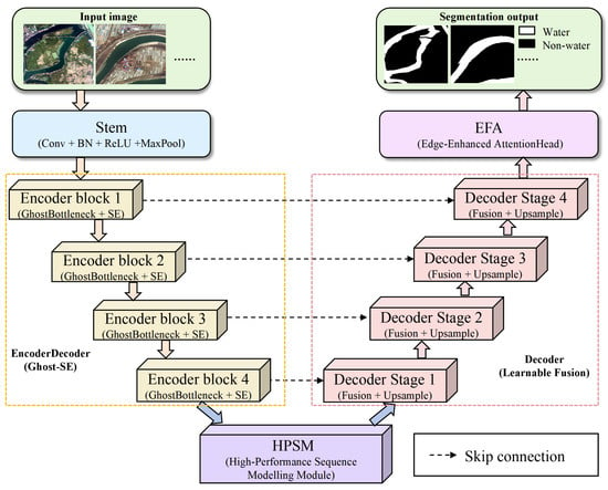
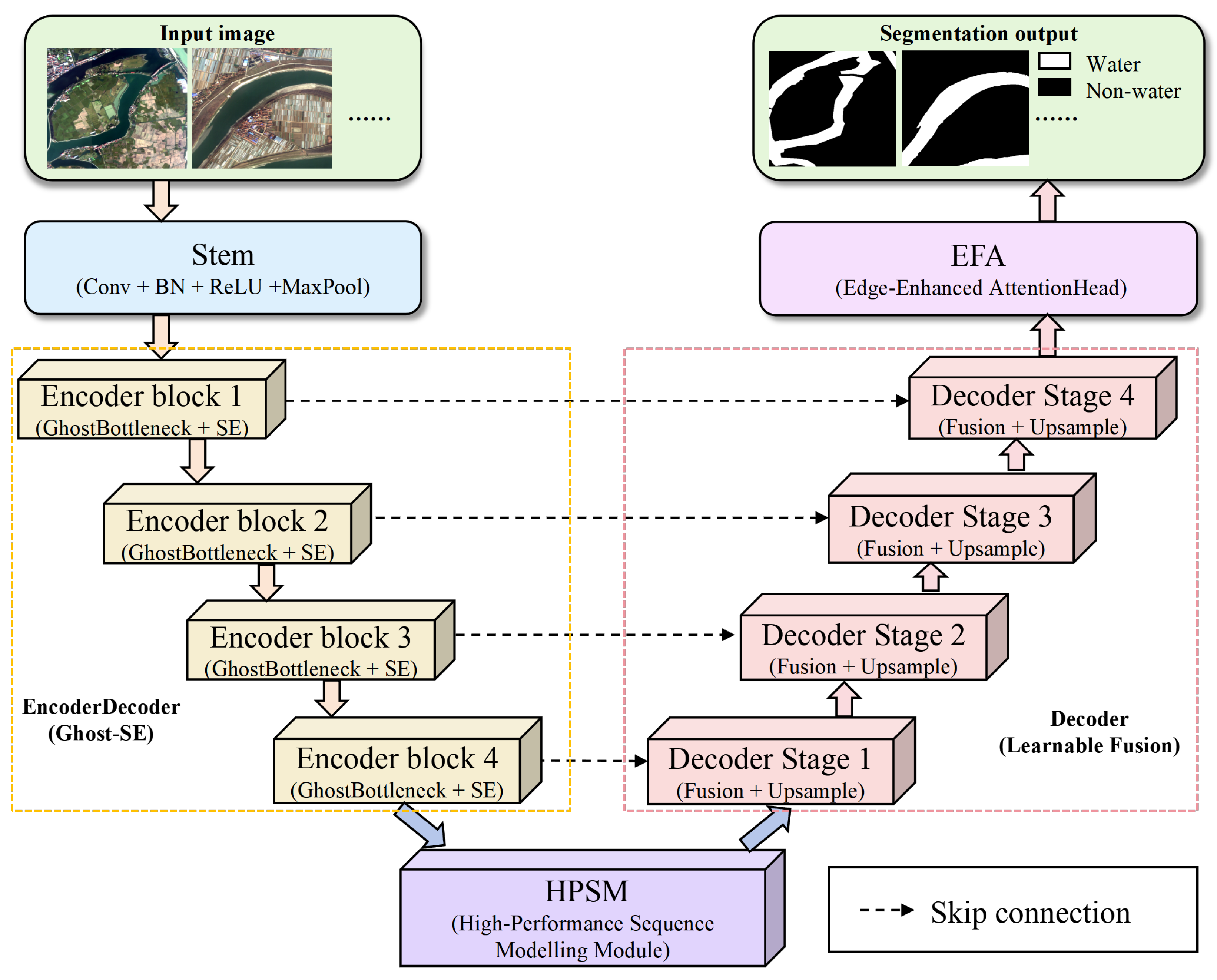
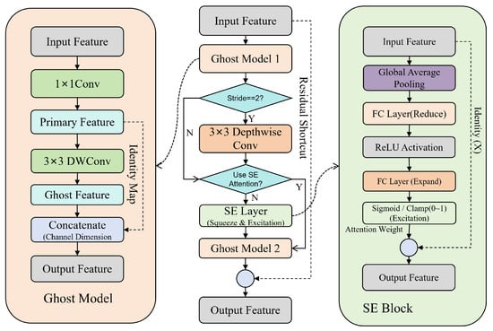
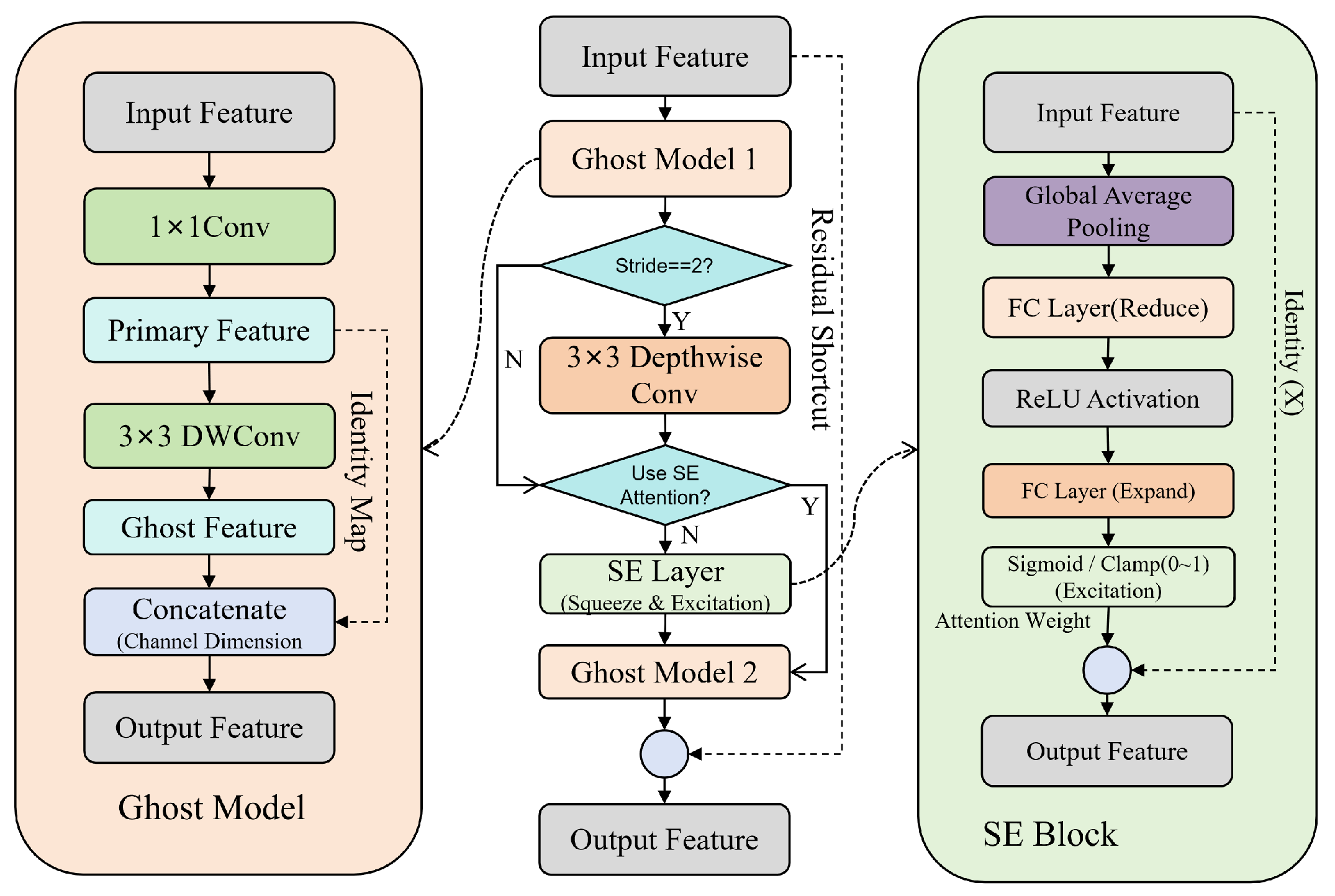
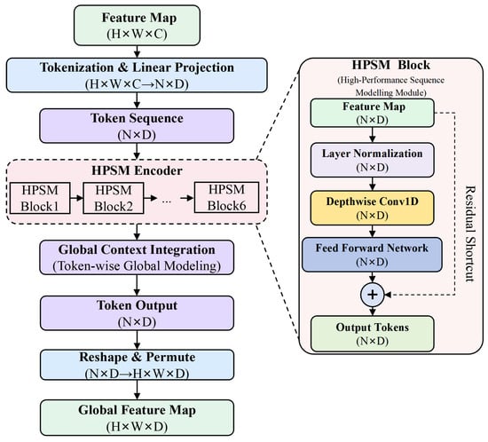
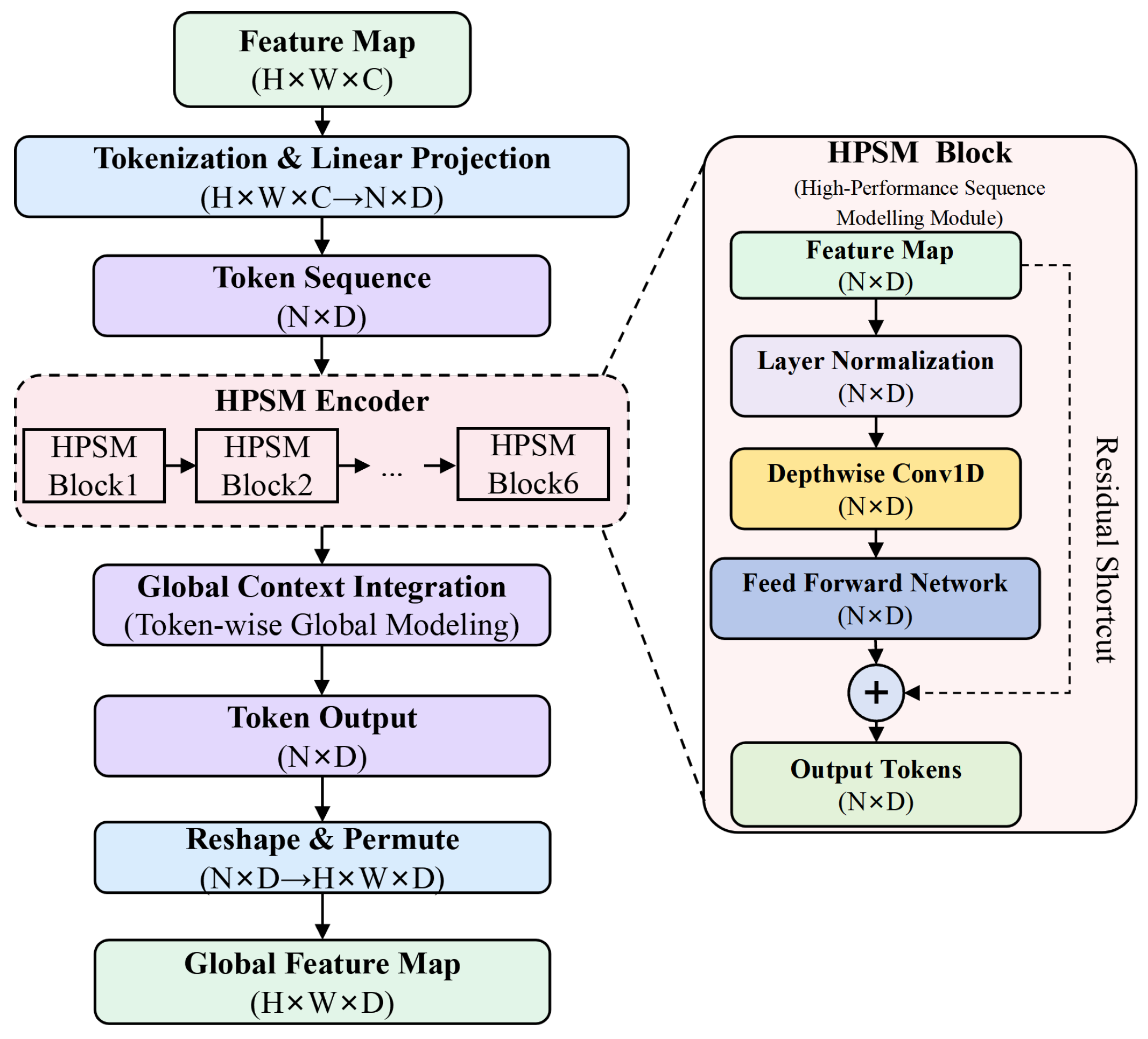
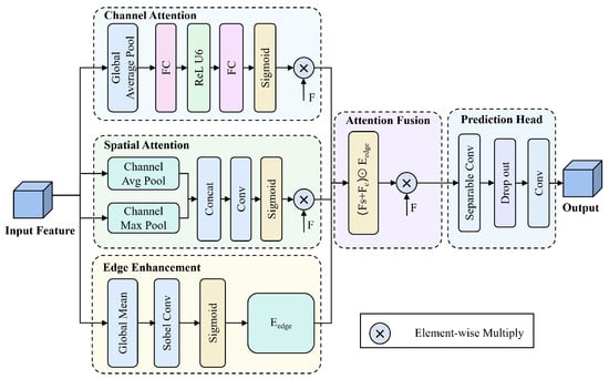
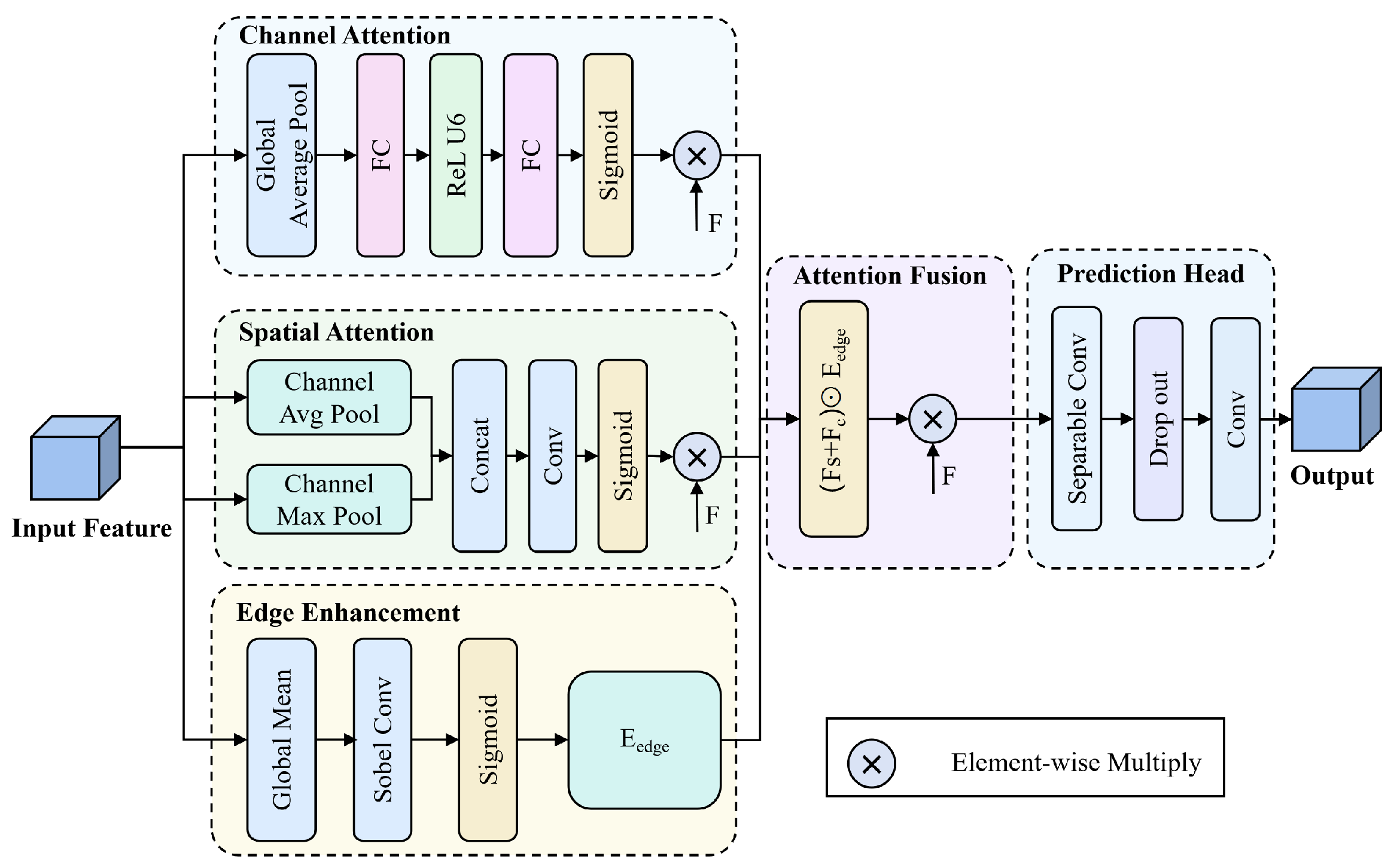
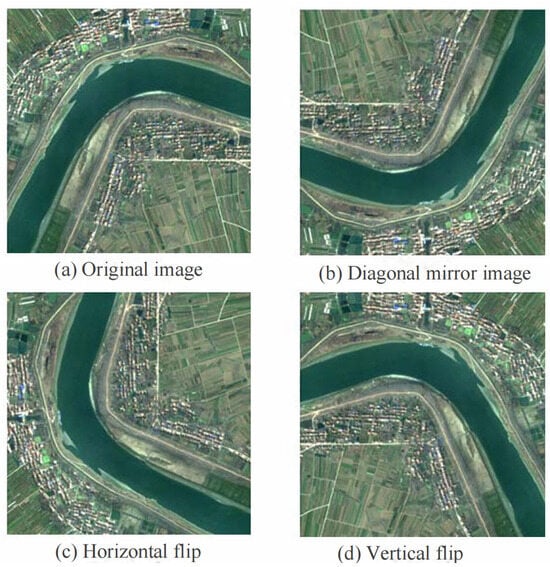
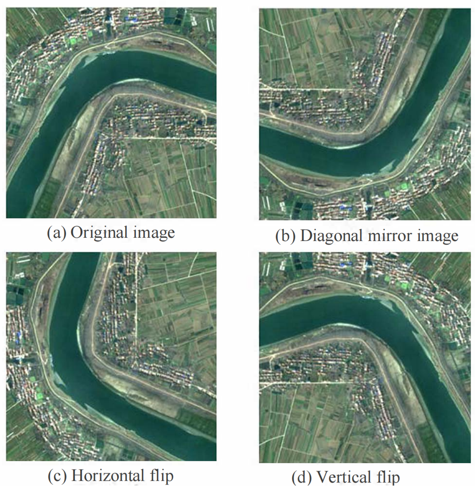
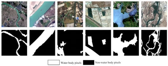
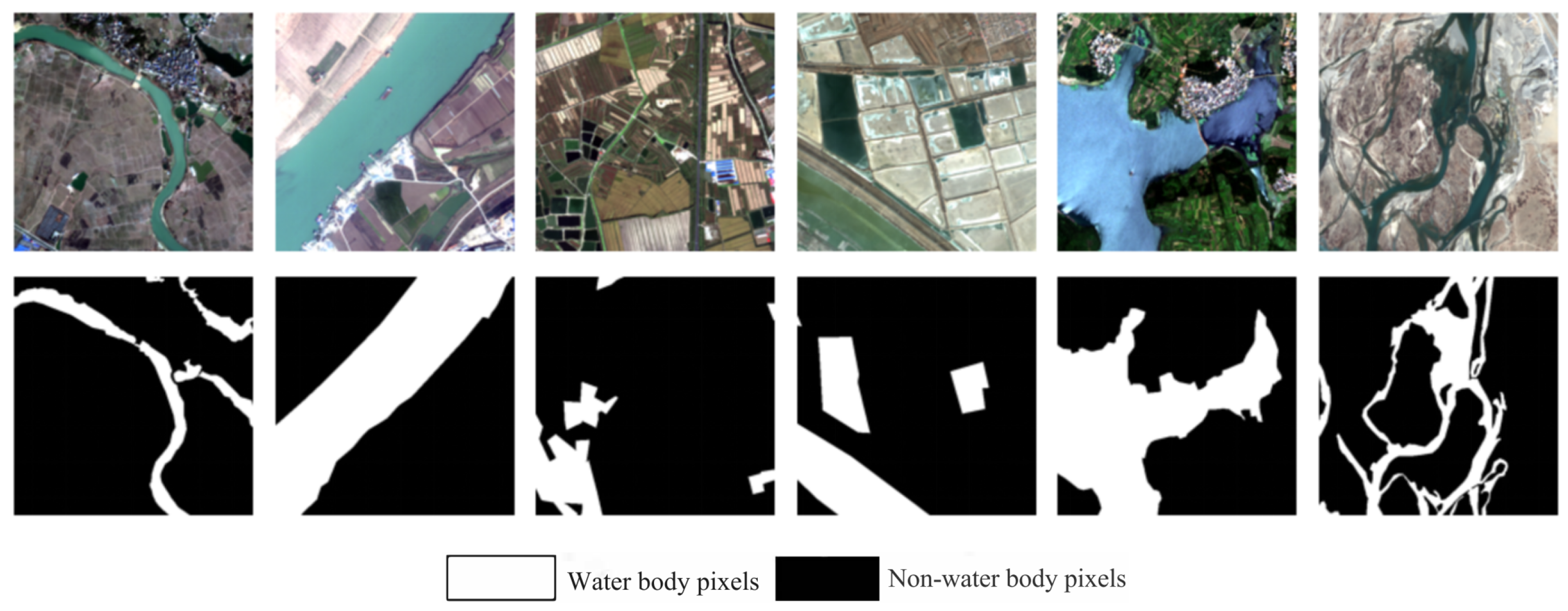
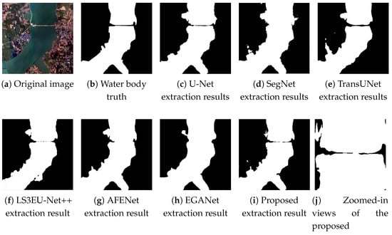
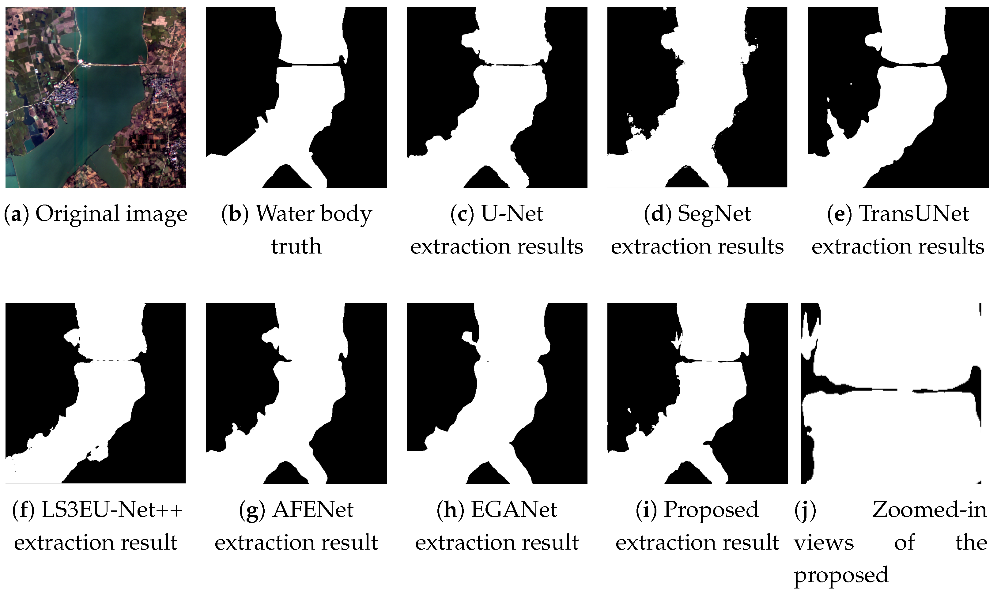
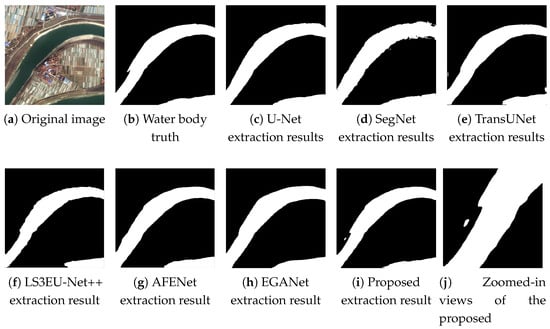
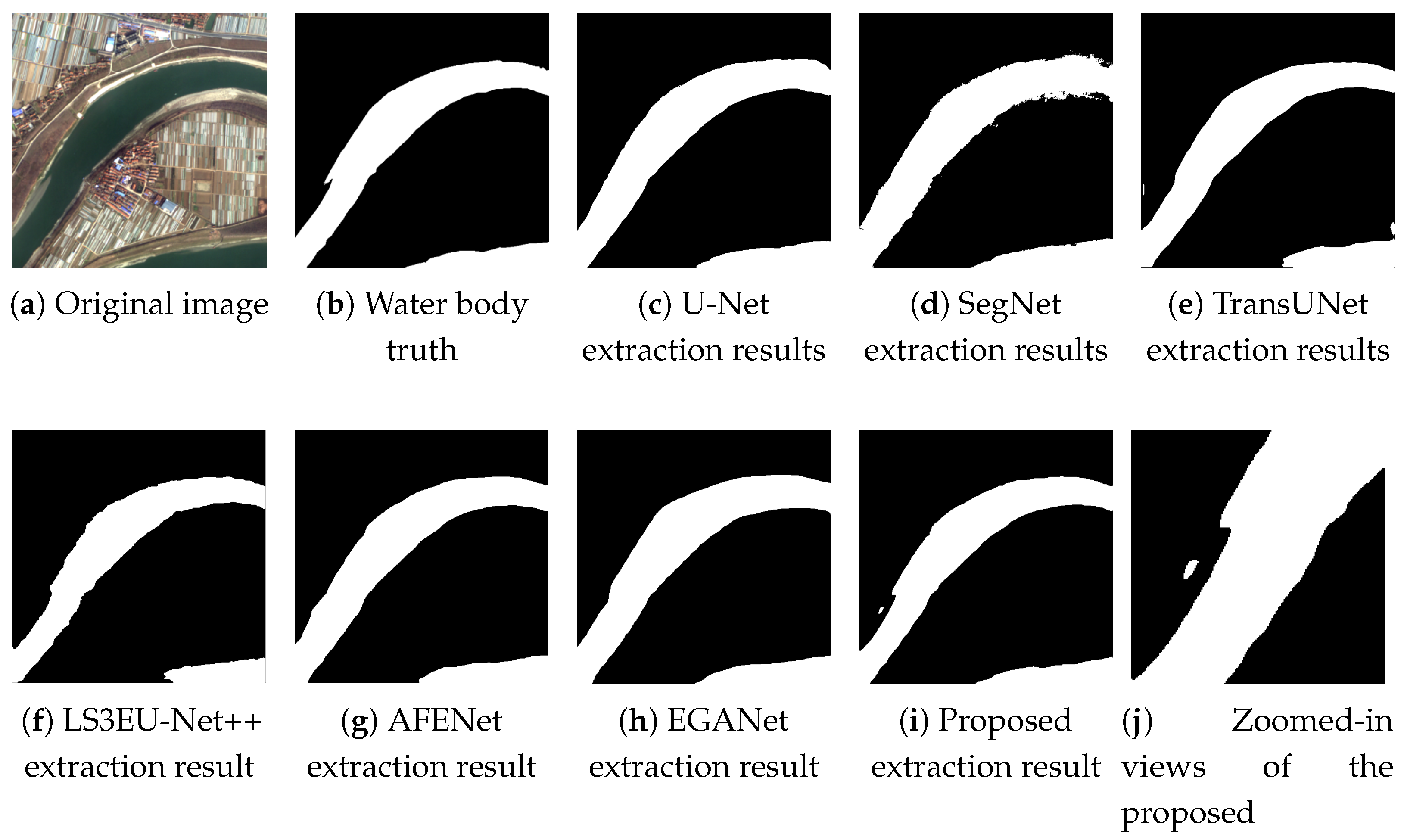
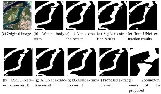
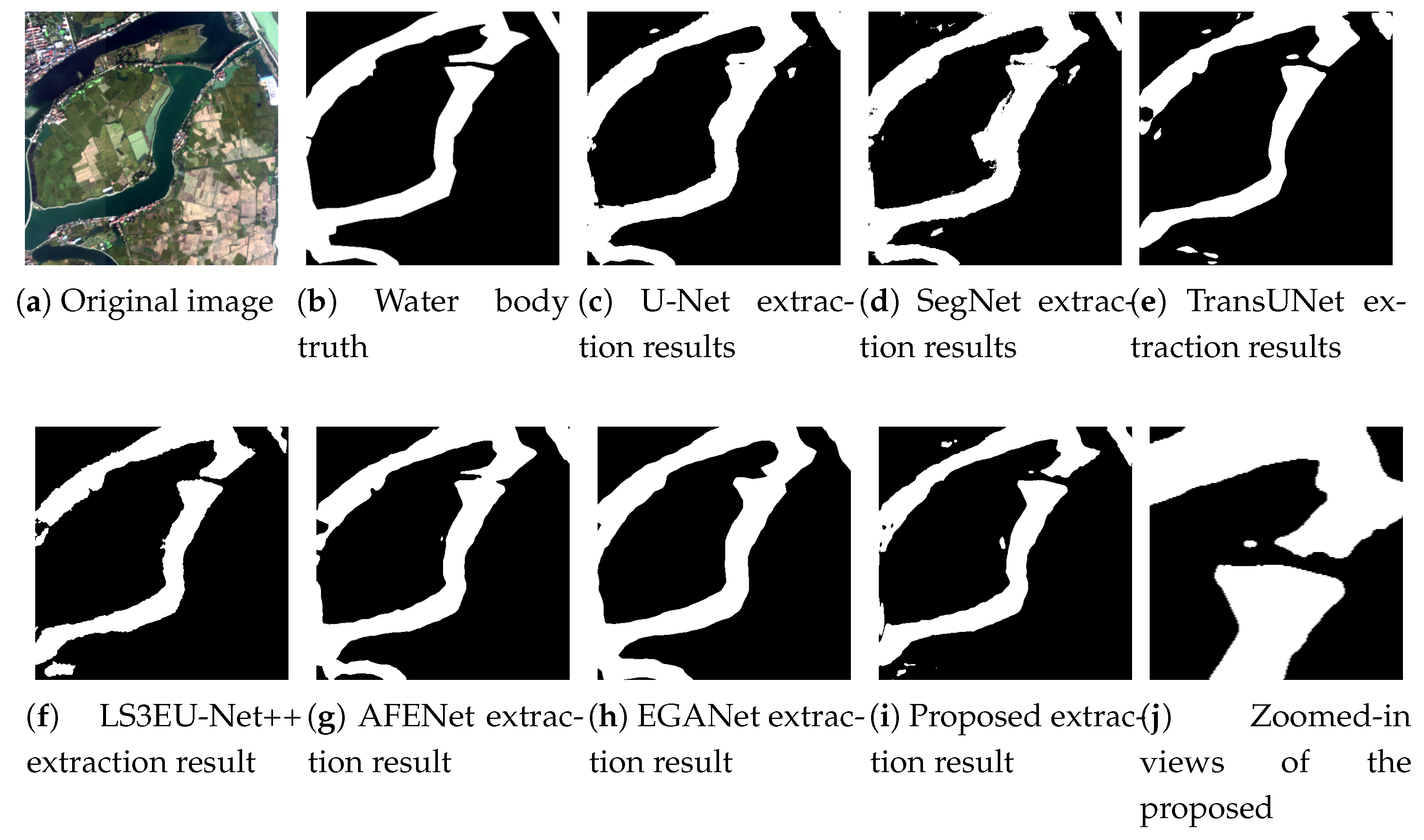
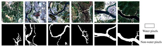
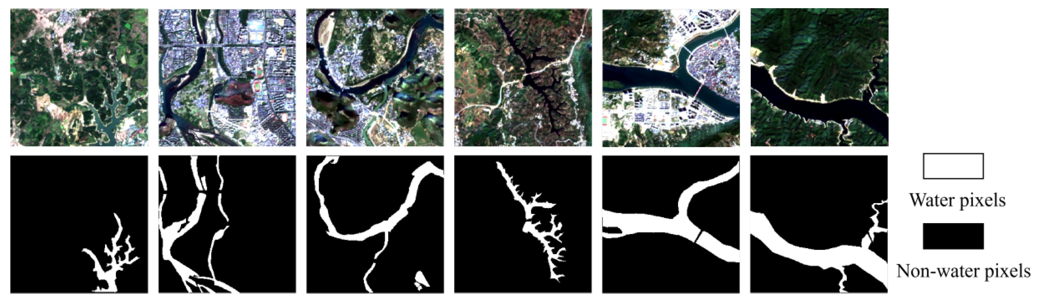
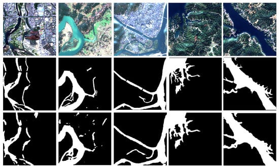
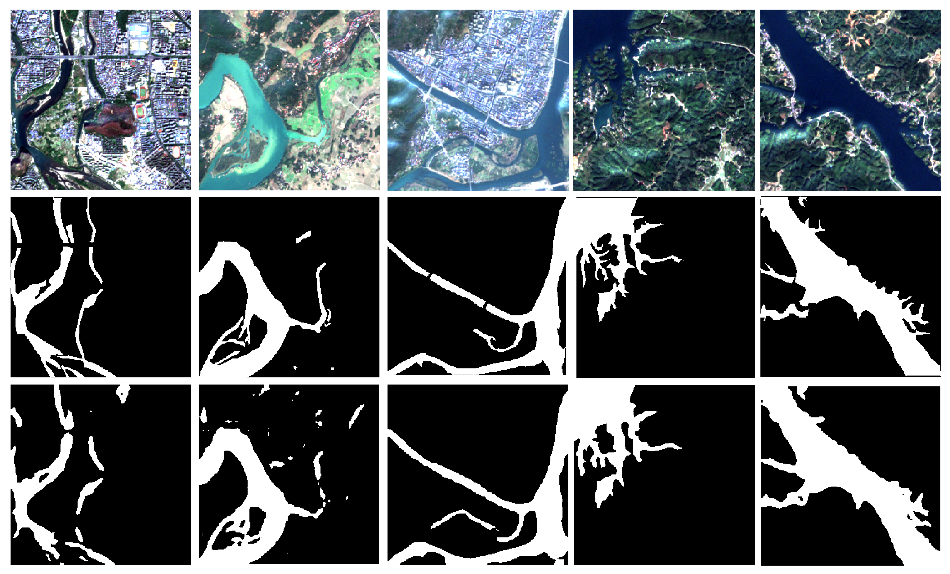
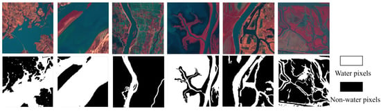
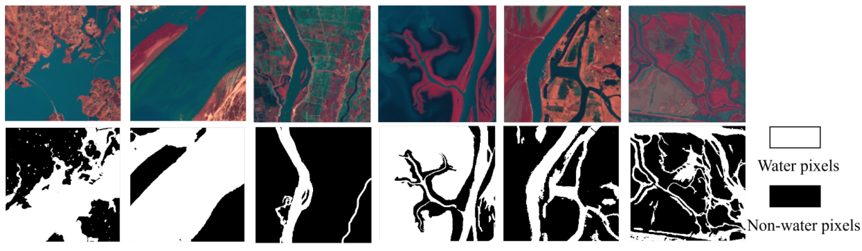
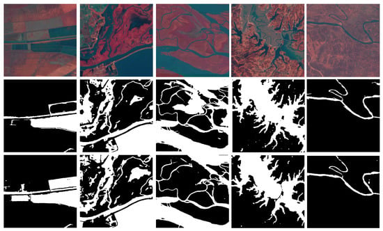
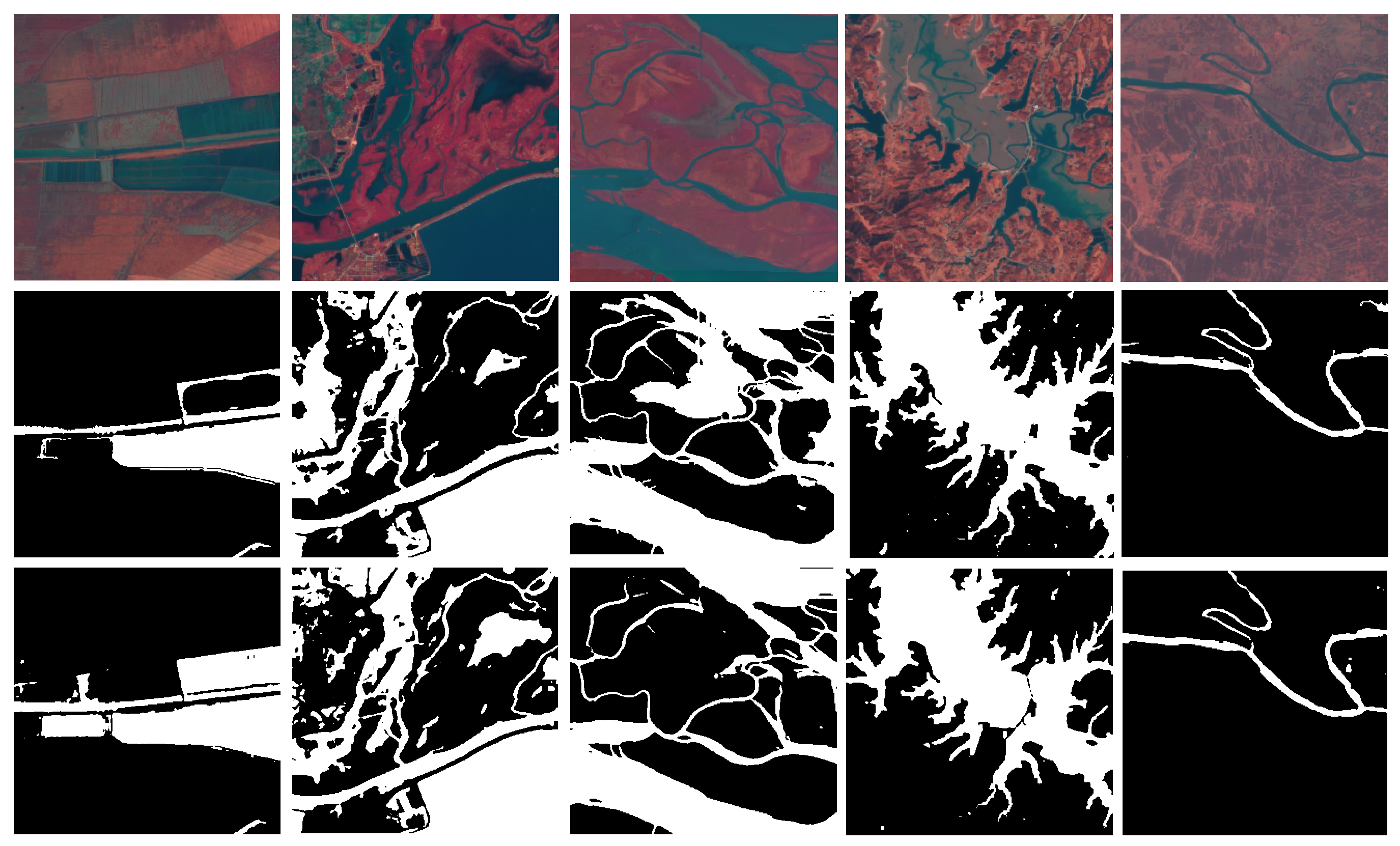

Disclaimer/Publisher’s Note: The statements, opinions and data contained in all publications are solely those of the individual author(s) and contributor(s) and not of MDPI and/or the editor(s). MDPI and/or the editor(s) disclaim responsibility for any injury to people or property resulting from any ideas, methods, instructions or products referred to in the content. |
© 2026 by the authors. Licensee MDPI, Basel, Switzerland. This article is an open access article distributed under the terms and conditions of the Creative Commons Attribution (CC BY) license.