


Highlights
What are the main findings?
- In maritime atmospheric environments, to effectively identify the over-the-horizon (OTH) propagation mechanisms of evaporation ducts (EDs), troposcatter and the transition states between them, we propose an identification method of OTH propagation mechanisms via measured path losses (PLs) over the northern South China Sea (SCS).
- To mitigate the short-term fluctuations of measured PLs and preserve the dominant PL variations, we utilize the method of exponentially weighted moving average (EWMA) to smooth the measured PLs.
- We propose an identification criterion for the troposcatter mechanism based on the PL prediction model for troposcatter of ITU-R P.617-5, as well as an identification criterion for the ED mechanism based on a Gaussian mixture model (GMM).
- Based on the proposed identification criterions, we also propose identification methods for the propagation mechanisms of both troposcatter and EDs.
What are the implications of the main findings?
- Compared with the evaporation duct height (EDH)-based identification method (EDHIM), the proposed method is independent of the forecasted EDH and provides quasi-real-time and more reliable identification of maritime OTH propagation mechanisms.
- The proposed method enables the maritime OTH communication systems to timely and sufficiently exploit ED by adjusting the transmit power and heights of transmit and receive antennas, and finally reduces the power consumption or increases the transmission rate.
Abstract
For the maritime over-the-horizon (OTH) propagation of electromagnetic (EM) waves in both C-band and X-band, evaporation ducts (EDs) and troposcatter are two dominant mechanisms, and they are significantly influenced by near-surface maritime atmospheric conditions. Most of the existing research treats ED and troposcatter as distinct mechanisms. However, one or multiple transitions will occur between them within one day, and there is no related research on the accurate identification of EDs and troposcatter. Therefore, we propose an identification method of OTH propagation mechanisms in maritime atmospheric environments based on measured path losses (PLs) in the northern South China Sea (SCS). Firstly, the method of exponentially weighted moving average (EWMA) is utilized to smooth the measured PLs. Secondly, the identification criterion and corresponding algorithm are proposed to identify the troposcatter mechanism. Thirdly, a Gaussian mixture model (GMM) combined with the expectation maximization algorithm are utilized to identify the ED mechanism and transition states. The performance of the proposed method is sufficiently validated via the measured PLs obtained from the northern SCS. The results show that compared with the intuitive method based on the forecasted evaporation duct height (EDH), the proposed method provides quasi-real-time and more reliable identification of maritime OTH propagation mechanisms.
1. Introduction
Maritime atmospheric environments, spanning from the near-surface maritime atmospheric layer to the troposphere, play a critical role in affecting the over-the-horizon (OTH) propagation of electromagnetic (EM) waves over the sea. Under such environments, evaporation ducts (EDs) and troposcatter frequently occur and constitute two dominant atmospheric propagation mechanisms, which enable the maritime OTH propagations and communications. Moreover, compared with Ultra High Frequency (UHF), Very High Frequency (VHF) and satellite communications, ED and troposcatter mechanisms make maritime OTH communications low-cost and high-rate by sufficiently exploiting the atmospheric conditions [1].
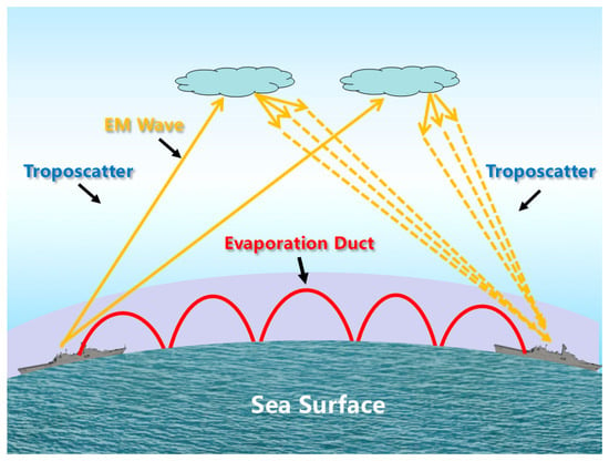
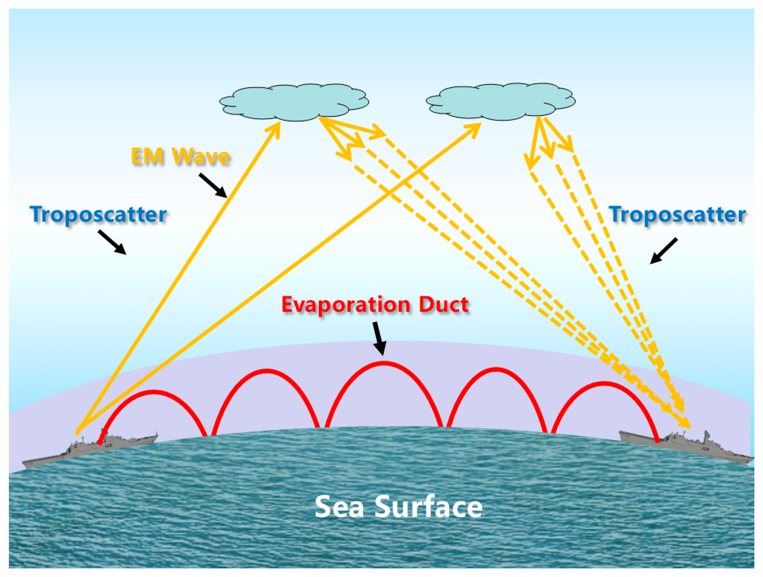
An ED is formed by the continuous evaporation and diffusion of water vapor from the sea surface, leading to high humidity near the surface and a rapid decrease in humidity with the increase in height [2,3,4]. This process leads to a negative refractivity gradient, forcing EM waves to bend toward the sea surface and then to be trapped within the ED layer [5,6,7]. Consequently, the propagation path losses (PLs) are significantly reduced, enabling OTH communication over distances of several hundred kilometers [8,9,10]. In contrast, the troposcatter mechanism relies on numerous scattering irregularities in the troposphere, e.g., turbulent eddies, clouds, warm fronts, cold fronts, and layered structures. These irregularities can scatter the microwave and millimeter wave, thereby also enabling OTH propagation [11,12,13,14]. As illustrated in Figure 1, the ED mechanism traps the EM waves within the ED layer, allowing OTH propagation with relatively lower PLs. In contrast, the troposcatter mechanism relies on scattering by the atmospheric irregularities in troposphere, resulting in relatively larger PLs. Moreover, the two mechanisms alternately dominate maritime OTH propagation under different maritime atmospheric conditions. It is worth mentioning that the applicable frequency region for both the ED and troposcatter mechanisms are C-band (i.e., 4.0 GHz–8.0 GHz) and X-band (i.e., 8.0 GHz–12.0 GHz), and EM waves with much higher or lower frequencies will lead to much bigger propagation PLs or even fail to achieve OTH propagation via EDs or troposcatter. As an example, the EM waves in the High Frequency (HF) band, e.g., 3 MHz–30 MHz, have wavelengths in the range of 100 m to 10 m, which are too long to be refracted by EDs or troposcatter; instead, they achieve OTH propagation through the ionospheric effect.
Figure 1.
Illustration of ED and troposcatter mechanisms in a maritime atmospheric environment.
Although EDs and troposcatter are two different OTH propagation mechanisms in maritime atmospheric environments, they will coexist in the transition state of OTH propagation. Specifically, in the transition states, the propagation mechanism will gradually transition from ED to troposcatter or from troposcatter to ED, and the signal strengths at the receiver via the channels of ED and troposcatter are comparable.
Moreover, according to the extensive experimental data obtained from cross-sea OTH communication links, except for the transition states, either EDs or troposcatter will be the dominant mechanism contributing to the measured PLs within a given time interval. Specifically, when the evaporation duct height (EDH) is relatively high (e.g., higher than 12 m) and the communication distance is relatively short (e.g., less than 100 km), EDs will be the dominant propagation mechanism. Conversely, when the EDH is lower or the OTH propagation link is longer (e.g., longer than 150 km), troposcatter becomes the dominant mechanism [8,10]; however, when the EDH is very high over the longer OTH link, EDs may still be the dominant mechanism.
Many existing works have investigated the mechanisms of EDs [6,7,8,9,10] and troposcatter [11,12,13,14]. In [6,7,8,9,10], the prediction of PLs over maritime OTH links based on the EDH are investigated for the ED mechanism, and the prediction accuracy has been validated via the measured PLs obtained from the constructed OTH links. Moreover, in [11,12,13,14], related models are utilized to predict the PLs in troposcatter mechanism. However, all the aforementioned works are conducted in a dominant propagation mechanism, either EDs or troposcatter, i.e., the mechanism remains unchanged over the specified maritime OTH links. In contrast, the extensive experiment data obtained from maritime OTH links have demonstrated that the dominant OTH propagation mechanism in a maritime atmospheric environment will transition between EDs and troposcatter one or multiple times each day. The transitions are mainly caused by the complex variations in maritime atmospheric conditions and diurnal fluctuations in EDH. Therefore, effectively identifying the maritime OTH propagation mechanisms from measured PLs is critical for capturing such complex variations as well as sufficiently utilizing EDs to improve the performance of maritime OTH communication systems.
However, the existing works [1,2,3,4,5,6,7,8,9,10,11,12,13,14] mainly focus on propagation modeling and prediction of propagation PLs based on environmental parameters, and the identification of OTH propagation mechanisms via measured PLs has not been sufficiently investigated. The evaporation duct height (EDH)-based identification method (EDHIM) can intuitively identify the mechanisms of EDs and troposcatter. In this method, by inputting the meteorological parameters (the relative humidity, sea surface temperature, wind speed components over the sea surface, etc.) released by the Global Forecast System (GFS) into the naval atmospheric vertical surface layer model (NAVSLaM) proposed by the US Naval Postgraduate School [15,16,17], EDHs can be forecasted in advance. However, in maritime atmospheric environments, the meteorological parameters used for forecasting EDHs are sometimes inaccurate. Accordingly, this intuitive method may lead to the misidentifications of the dominant propagation mechanism. It is also worth mentioning that the measured PLs obtained by maritime OTH communication systems may contain abnormally large or small outliers caused by obstructions from passing ships, antenna vibrations under high wind conditions, severe co-channel interference, etc., which will degrade the accuracy of mechanism identification. Nevertheless, none of the related literature [1,2,3,4,5,6,7,8,9,10,11,12,13,14] smoothed the measured PLs.
To address the aforementioned issues, this paper proposes a method to identify the OTH propagation mechanisms based on measured PLs in the maritime atmospheric environment of the northern South China Sea (SCS). Firstly, we exploit the method of exponentially weighted moving average (EWMA) to reduce the influence of abnormal fluctuations from measured PLs obtained from the constructed maritime OTH links. Then, we propose the identification criterion and corresponding algorithm to identify the troposcatter mechanism. Subsequently, from the remaining measured PLs, we utilize a Gaussian mixture model (GMM) together with the expectation maximization algorithm to identify the ED mechanism as well as the transition states between the troposcatter and ED mechanisms. Finally, a large amount of measured PLs in X-band obtained from the constructed OTH links constructed in the northern SCS are utilized to sufficiently validate the performance of the proposed identification method. It is worth mentioning that the proposed identification method does not assume a strict physical separation between the ED and troposcatter mechanisms. Instead, it identifies the dominant propagation mechanism together with the transition state, i.e., EDs and troposcatter coexist during maritime OTH propagation, via the measured PLs.
Consequently, compared with the intuitive identification method EDHIM, the proposed method is independent of the forecasted EDH and provides quasi-real-time and more reliable identification of maritime OTH propagation mechanisms. More importantly, the proposed method enables maritime OTH communication systems to timely and sufficiently exploit EDs by reducing the transmit power as well as the heights of the transmit and receive antennas, thereby leading to reduced power consumption or increased transmission rate. Furthermore, when troposcatter is identified as the dominant propagation mechanism, the transmit power and antenna heights should be increased to compensate for the larger PLs.
2. PL Prediction Model in Troposcatter Mechanism
The predicted PL in the troposcatter mechanism is obtained by summing the median basic propagation loss exceeded for 50% of the time, i.e., L(50), the sea surface reflection loss Lr, the atmospheric absorption loss LA, and the antenna medium coupling loss Lc [18,19,20,21,22].
Firstly, the median basic propagation loss exceeding 50% of the time is
In (1), M denotes the meteorological parameter, f is the operating frequency of OTH communication system in MHz, d represents the length of OTH link in km, and θ is the minimum scattering angle. The term accounting for the influence of the common volume bottom height, i.e., N (H, h), is determined by
In (2), H = 10−3 θd/4 is the minimum scattering height in km. h = 10−6 θ2ae/8 denotes the height of the lowest scattering point over the sea surface in km, where ae is the effective earth radius, and it is determined by
In (3), Ns denotes the surface atmospheric refractivity exponent, which is defined as the average of the corresponding values at the transmitter and receiver of a practical OTH communication system. Finally, the parameter γ in (2) represents the atmospheric structure parameter.
Secondly, the sea surface reflection loss Lr is a function of the antenna height, wavelength, communication distance, beam geometry and circuit parameters. In this paper, Lr is set to 0.5.
Thirdly, the atmospheric absorption loss LA is
In (4), A(d) and B(f) respectively denote the quantities associated with the transmit distance and frequency, and they are respectively determined by
Fourthly, the antenna medium coupling loss Lc is determined by
where Gt and Gr are the gains of the transmit and receive antennas in decibels isotropic (dBi), respectively.
Finally, the predicted PL in the troposcatter mechanism is
3. Acquisition and Preprocessing of Measured PLs
3.1. Acquisition of Measured PLs
In practical maritime OTH communication systems, the measured PLs are determined by the transmit power, the gains of transmit and receive antennas, the received signal strength indicator (RSSI) and the system loss, i.e.,
In (9), PLme denotes the measured PLs in decibels (dB), and Pt represents the transmit power of the maritime OTH communication system in decibels milliwatt (dBm). Gt and Gr respectively denote the gains of transmit and receive antennas in dBi, and RSSI is the received signal strength indicator in dBm. Finally, Sl denotes the system loss in dB.
3.2. Data Smoothing via the EWMA Method
It is worth noting that the measured PLs obtained from the constructed OTH links will contain abnormal fluctuations which may be caused by obstructions from passing ships, antenna vibrations under high wind conditions, severe co-channel interference, etc. Moreover, the abnormal fluctuations may affect the reliability of propagation mechanism identification. Therefore, the EWMA method [23,24] is applied to smooth the measured PLs as well as reduce the influence of short-term fluctuations. Since the abnormal variations caused by passing ships or antenna vibration typically appear as short-term fluctuations, the EWMA method can effectively mitigate their influence while preserving the dominant variation characteristics of the measured PLs. The smoothed PLs, denoted as , are determined as follows:
In (10), is the measured PL at the i-th data sample, where i = 1, 2, …, I, and I represents the total number of measured PL samples. The parameter α is the smoothing factor, where 0 < α < 1. In this paper, based on the measured PL characteristics, α is set to 0.3, which provides a balance between mitigating the short-term fluctuations and preserving the dominant variations associated with different propagation mechanisms, i.e., EDs, troposcatter and the transition states between them. Specifically, a smaller value of α may lead to excessive smoothing and weakening of the variation characteristics associated with the transitions between propagation mechanisms, where a larger value may retain more short-term fluctuations that will affect the accuracy of mechanism identification.
3.3. Time-Averaged PL Computation
For the measured PLs after data smoothing via the EWMA method, the time-averaged PL is computed in an interval of Δt. Assume that the p-th (1 ≤ p ≤ P) time interval contains Jp samples of the measured PLs after data smoothing, where P is the total number of time intervals. Then, the time-averaged measured PL within the p-th time interval, i.e., , is
In (11), denotes the j-th (1 ≤ j ≤ Jp) smoothed PL sample within the p-th time interval. Moreover, Jp is the number of smoothed PL samples within the p-th time interval. In practical maritime OTH propagation scenarios, an excessively large value of Δt may contain multiple transitions between ED and troposcatter mechanisms, thereby degrading the accuracy of mechanism identification. Additionally, a Δt with too small value will increase the computational complexity of mechanism identification without significant performance improvements. More importantly, over the specified OTH link of a short time interval (e.g., Δt = 5 min), since the maritime meteorological parameters (the relative humidity, sea surface temperature, wind speed components over the sea surface, etc.) for forecasting EDH almost remain unchanged, the EDH also exhibits negligible variations. Therefore, Δt should not be too small. In practical applications, the recommended range for Δt is 10 min to 30 min.
4. Identification Method of Maritime OTH Propagation Mechanisms
The troposcatter mechanism is relatively insensitive to the variations in maritime meteorological conditions, so the corresponding propagation PLs remain relatively stable. Based on this characteristic, the proposed identification method firstly identifies the troposcatter mechanism, and then identifies the ED mechanism, and finally identifies the transition states between the ED and troposcatter mechanisms from the remaining measured PLs.
4.1. Proposed Identification Method for Troposcatter Mechanism
For the n-th (1 ≤ n ≤ N) OTH communication reference link, the root mean square error (RMSE) between the predicted and measured PLs within the k-th time interval is given by
where yh,n is the h-th (1 ≤ h ≤ H) measured PL over the n-th (1 ≤ n ≤ N) reference link, and H represents the total number of measured PL samples. Moreover, PLpre denotes the predicted PL obtained by the PL prediction model for troposcatter of the n-th reference link. For a reference link with length ln (1 ≤ n ≤ N), the threshold of the difference between the predicted and measured PLs is defined as rounding up the maximum RMSE in K different time intervals associated with this reference link, i.e.,
In (13), RMSE1,n, …, RMSEK,n denote the RMSEs corresponding to the K different time intervals over reference link ln.
Furthermore, for a constructed maritime OTH link with length d, the threshold of the difference between the predicted and measured PLs, i.e., , is defined as follows:
In (14), , …, denote the thresholds of differences between the predicted and measured PLs corresponding to the reference links with lengths l1, l2, …, lN, respectively. Furthermore, , , …, respectively represent the corresponding bias correction associated with , …, . In practical scenarios, (1 ≤ n ≤ N) can be selected from the interval (0, ) to account for the model error. As a special case, if all the N constructed OTH links with lengths l1, l2, …, lN are selected as the N reference links, we have Δ1 = Δ2 = … = ΔN = 0.
As the length of a specified OTH communication link may not be exactly the same as those of the reference links, the corresponding threshold (i.e., ) will be approximately determined by the following procedure. According to (14), the interval [50 km, lN] is firstly partitioned into multiple subintervals via the midpoints of adjacent reference link lengths. If the length of a given link, i.e., d, is closest to that of the reference link lq (2 ≤ q ≤ N − 1), then d is considered to fall within the interval [(lq−1 + lq)/2, (lq + lq+1)/2]. Accordingly, the threshold for this link is considered as + Δq. Specifically, when 50 km ≤ d ≤ l1, the threshold ΔPL is set to ; when (lN−1 + lN)/2 < d ≤ lN, the threshold is set to . For the case where d > lN, the threshold is set to . Here β (β > 1) is a scaling factor determined by the length of the maritime OTH link, and it is used to expand the threshold range for links longer than the reference link with the maximum length, reflecting increased uncertainty in the PL of OTH propagation over longer links.
For a maritime OTH communication link with length d (l1 ≤ d ≤ lN), there always exists a gap between the predicted PLs in the troposcatter mechanism and the measured PLs. Specifically, the threshold of the difference between the predicted and measured PL is determined according to (14). If the time-averaged measured PL, i.e., in (11), falls within the interval [PLpre − , PLpre + ], the dominant propagation mechanism during the p-th time interval is identified as troposcatter. If is not within [PLpre − , PLpre + ], the corresponding dominant mechanism will be either an ED or a transition state between an ED and troposcatter.
Then, the following criterion is proposed to identify the propagation mechanism of a maritime OTH communication link within a specified time interval:
In (15), PLpre, and are determined by (8), (11), and (14), respectively. Based on the proposed criterion in (15), the identification method of the troposcatter mechanism is shown in Algorithm 1.
| Algorithm 1: Identification Method for the Troposcatter Mechanism |
| 1: Compute the predicted PL PLpre and the time-averaged measured PL within the p-th time interval according to (8) and (11), respectively. 2: Compute the RMSE between the predicted and measured PLs for each reference link via (12). 3: Determine the threshold ΔPL for each OTH communication link with length d by (13) and (14). 4: for each time interval p-th do 5: if then 6: Identify the dominant propagation mechanism as troposcatter. 7: else 8: Identify the dominant propagation mechanism as either ED or transition state. 9: end if 10: end for 11: Return the identified propagation mechanism for each time interval. |
4.2. Proposed Identification Method for ED Mechanism
After the troposcatter mechanism is identified, there remain some time intervals during which the measured PLs are significantly lower than the predicted PL, but do not fall within [PLpre − , PLpre + ]. Such time intervals will be either the ED mechanism or transition states, including transitions from ED to troposcatter and from troposcatter to ED. To further improve the accuracy of maritime OTH propagation mechanism identification, GMM [25,26,27] is utilized to identify the ED mechanism from the remaining time intervals.
Firstly, the difference between the time-averaged measured PL in the p-th time interval (i.e., ) and the predicted PL (i.e., PLpre) is computed to quantitatively characterize the deviation of the PL prediction model in the troposcatter mechanism, i.e.,
Here it is worth noting that if the interval Δt is too small, the variation of rp is almost negligible. Moreover, an excessively large Δt may contain multiple transitions between the ED and troposcatter mechanisms. Accordingly, Δt should be set to an appropriate value so that the ED and troposcatter mechanisms can exhibit distinct characteristics in rp. When an ED occurs over the sea surface, the time-averaged measured PLs will be significantly reduced. Consequently, is much smaller than PLpre.
The distribution of rp under a relatively stable propagation mechanism can be approximately modeled by a Gaussian distribution. Since the maritime OTH propagation mechanisms comprise troposcatter, ED and the transition states between them, rp is composed of statistical distributions corresponding to multiple propagation mechanisms. Specifically, the troposcatter and ED represent relatively stable propagation mechanisms over certain time intervals, during which the corresponding values of rp approximately obey the Gaussian distribution. In contrast, during the transition state, the statistical distribution of rp is influenced by the coexistence of the ED and troposcatter mechanisms, resulting in a wider statistical distribution than the ED mechanism.
Therefore, a GMM consisting of two Gaussian components is adopted to fit the remaining rp samples. The two Gaussian components are used to describe the statistical distributions of the ED mechanism and the transition states, respectively. The reason for this is that regarding the components of EDs and transition states as Gaussian is an empirical approximation rather than an a priori assumption. In the ED mechanism, the energy of electromagnetic waves is trapped within the ED layer, and the received signal is dominated by a coherent ducted component, so the short-term fluctuation of path losses is commonly approximated as Gaussian. Because the measured PLs are notably lower than those predicted by the troposcatter propagation model, rp forms a Gaussian component with a strongly negative mean. In the transition state, an ED and troposcatter coexist, and the signal strengths at the receiver respectively via the ED and troposcatter channels are comparable, so the distribution of rp becomes broader; moreover, this broader distribution is still approximated by a Gaussian component with a larger variance. Therefore, the narrower ED and broader transition state are an observed feature of the measured residuals, not a theoretical claim.
When an ED is the dominant OTH propagation mechanism, the measured PLs are notably lower than the predicted PLs, resulting in smaller values of rp. In contrast, during the transition state, the received signals are affected by both the ED and troposcatter mechanisms, resulting in a wider distribution of rp than the ED mechanism. It is worth mentioning that the GMM does not assume that the transition state itself is bimodal; instead, it is utilized to separate the narrow distribution of the ED from the broader distribution of the transition state statistically.
Accordingly, the probability density function of rp can be expressed as
where πm is the mixing weight of the m-th Gaussian component, satisfying 0 < πm < 1 and . Moreover, the parameters μm and denote the mean and variance of the m-th Gaussian component, respectively. Finally, the function represents the one-dimensional Gaussian probability density function, which is defined as
During the stage of model training, the K-means clustering algorithm [28] is applied to the set of rp values to obtain an initial partition, thereby providing initial estimates of the parameters πm, μm and in GMM. Since the OTH propagation mechanism corresponding to each rp sample is unknown, the expectation maximization algorithm [29] is subsequently utilized to perform the unsupervised parameter estimation of the GMM. During the parameter updating, the posterior probability of each rp belonging to a specific propagation mechanism is simultaneously estimated. The iteration process is summarized as follows:
(1) based on the current parameter estimates, the posterior probability that rp belongs to the m-th propagation mechanism is evaluated as
(2) using the posterior probabilities obtained from (19), parameters in GMM, i.e., πm, μm and , are respectively updated as follows:
(3) when the variation of the parameters between two consecutive iterations is smaller than or equal to a given threshold (e.g., 10−3), the parameters are regarded as having converged, and the iteration process is terminated.
After πm, μm and converge, the Gaussian component with the smallest mean value μm is identified as the ED mechanism, since the measured PLs in the ED mechanism are much smaller than those in transition states. Subsequently, for the p-th time interval, the posterior probability that rp belongs to the ED component, i.e., PED(p), is computed. Based on the value of PED(p), the identification criterion for the ED mechanism is
In (23), Pth is the threshold of PED(p). In this paper, Pth is set to 0.5, which is based on the Bayesian decision rule for the minimum error rate. Besides, the ED and transition state components in the GMM are assigned equal prior weights. The reason is that in a two-class classification problem with equal prior probabilities and symmetric misclassification costs, the posterior probability of 0.5 serves as the optimal decision boundary that minimizes the overall error probability [27,30]. If PED(p) in a given time interval satisfies PED(p) ≥ Pth, the dominant OTH propagation mechanism during this time interval is identified as an ED; otherwise, it is identified as a transition state, i.e., from ED to troposcatter or troposcatter to ED.
In summary, the details of the proposed identification method for the ED mechanism are given in Algorithm 2.
| Algorithm 2: Identification Method for the ED Mechanism |
| 1: Compute the predicted PL PLpre and the time-averaged measured PL within the p-th time interval according to (8) and (11), respectively. 2: Compute the difference rp between and PLpre by (16). 3: Initialize the parameters of the GMM, including πm, μm and . 4: Apply the K-means clustering algorithm to the set of rp values to obtain an initial partition. 5: for each iteration do 6: Compute the posterior probability for each rp by (19). 7: Update the parameters of the GMM via (20)–(22). 8: if the variation of the parameters between two consecutive iterations is smaller than a given threshold then 9: Terminate the iteration process. 10: end if 11: end for 12: Identify the Gaussian component with the smallest mean value μm as the ED mechanism. 13: for each time interval p-th do 14: Compute the posterior probability PED(p) that rp belongs to the ED component. 15: if PED(p) ≥ Pth then 16: Identify the dominant propagation mechanism as an ED. 17: else 18: Identify the dominant propagation mechanism as a transition state. 19: end if 20: end for 21: Return the identified dominant propagation mechanism for each time interval. |
Finally, according to the identification results, the maritime OTH communication systems will adopt corresponding parameter adjustment strategies. Specifically, when an ED is identified as the dominant mechanism, because more energy of EM waves can be trapped in the ED layer, the transmit power as well as the heights of the transmit and receive antennas should be reduced, thereby reducing the power consumption or increasing the transmission rate. In contrast, when troposcatter becomes the dominant mechanism, to address the larger propagation PLs, the transmit power as well as the heights of the transmit and receive antennas should be increased.
5. Experimental Verification
5.1. Cross-Sea Experiment for OTH Communications
From 13 June to 15 July 2024, the maritime OTH communication experiments were conducted in the coastal regions near Jizhao Bay, Yangxi, and Yangjiang in Guangdong Province, as well as Wenchang in Hainan Province. During the experiments, the measured PLs in X-band were obtained from the self-developed maritime OTH communication systems whose parameters are given in Table 1.
Table 1.
System parameters.
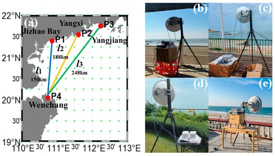
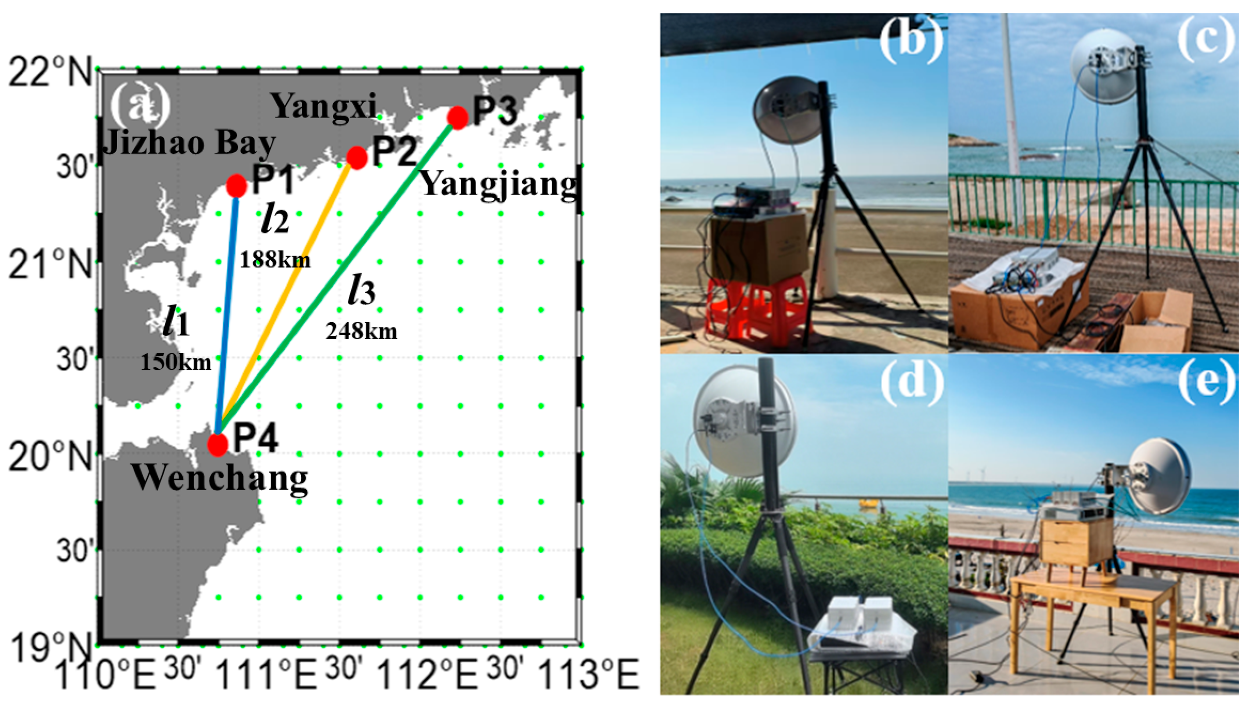
Figure 2a shows the experiment locations and three constructed OTH communication links, P1P4, P2P4, and P3P4, with lengths of 150 km, 188 km and 248 km, respectively. Moreover, Figure 2b–d illustrate the deployments of self-developed maritime OTH communication systems. Specifically, the transmitters were respectively deployed at P1 (21°39′N, 110°40′E) in Jizhao Bay, Zhanjiang, Guangdong Province; P2 (21°53′N, 111°59′E) in Yangxi, Guangdong Province; and P3 (21°44′N, 112°24′E) in Yangjiang, Guangdong Province. Figure 2d exhibits the receiver deployed at P4 (20°04′N, 110°75′E) in Wenchang, Hainan Province. Finally, a large amount of measured PLs were obtained from the three constructed OTH communication links and then utilized to sufficiently validate the accuracy of the proposed identification method.
Figure 2.
Experimental setup and geographic locations of the three OTH communication links. (a) Geographic distribution of the experiment locations and the OTH links; (b) Jizhao Bay; (c) Yangxi; (d) Yangjiang; (e) Wenchang.
5.2. Threshold Determination for PL Difference
According to (11), we can obtain a time-averaged measured PL with a time interval (i.e., Δt) of 10 min after data smoothing by EWMA. In this paper, as shown in Figure 2a, three maritime OTH communication links with lengths of 150 km, 188 km and 248 km are selected as the reference links l1, l2 and l3, respectively.
Note that the value of the thresholds of difference between the predicted and measured PLs for the reference links directly affects the identification performance of the proposed method. Specifically, a larger threshold will yield a much wider decision band for the troposcatter mechanism, which makes the proposed method misidentify an ED or a transition state as troposcatter. On the contrary, a smaller threshold will narrow the decision band and make the proposed method misidentify the intervals of troposcatter as EDs or transition states.
Therefore, to address this issue, the reference intervals used for evaluating the RMSE between the predicted and measured PLs over the OTH links with lengths of 150 km, 188 km and 248 km are the selected intervals, in which troposcatter is definitely the dominant propagation mechanism according to the physical characteristics of the propagation PLs in the troposcatter mechanism. Then, according to Formula (13), the maximum RMSE values of the aforementioned reference intervals are rounded up as the threshold of difference between the predicted and measured PLs for the reference links. Consequently, the determined threshold is relatively conservative, and it can sufficiently represent the real fluctuations of the troposcatter mechanism.
For the reference link of 150 km, during 07:00–10:00 and 19:00–21:00 on 16 June 2024, the RMSEs between the predicted and measured PLs are 9.24 dB and 7.95 dB, respectively. In addition, during 00:00–06:00 on 4 July 2024, the RMSE has a value of 4.05 dB; during 01:00–09:00 and 15:00–20:00 on 6 July 2024, the RMSEs are 3.85 dB and 9.42 dB, respectively. Finally, during 00:00–06:00 on 8 July 2024, the RMSE is 6.77 dB. Therefore, according to (13), the threshold of difference between the predicted and measured PLs for the reference link of 150 km is = ⌈max {9.24, 7.95, 4.05, 3.85, 9.42, 6.77}⌉ = 10 dB.
Moreover, for the reference link of 188 km, during 00:00–06:00 on 22 June 2024, the RMSE between the predicted and measured PLs is 5.77 dB. Similarly, during 10:00–12:00 on 17 June 2024, the RMSE is 6.89 dB; during 00:00–03:00 on 18 June 2024, the RMSE is 4.47 dB; and during 03:00–06:00 on 27 June 2024, the RMSE yields a value of 4.63 dB. Finally, during 00:00–06:00 on 3 July, the RMSE is 5.65 dB. Thus, according to (13), the threshold of difference between the predicted and measured PLs for the reference link of 188 km is = ⌈max {5.77, 6.89, 4.47, 4.63, 5.65}⌉ = 7 dB.
Finally, for the reference link of 248 km, during 03:00–06:00 and 09:00–12:00 on 9 July 2024, the RMSEs between the predicted and measured PLs are 3.81 dB and 5.68 dB, respectively. In addition, during 00:00–06:00 on 10 July 2024, the RMSE is 2.85 dB; during 06:00–09:00 and 21:00–23:59 on 11 July 2024, the RMSEs are 4.12 dB and 4.44 dB, respectively. Consequently, according to (13), the threshold of difference between the predicted and measured PLs for the reference link of 248 km is = ⌈max {3.81, 5.68, 2.85, 4.12, 4.44}⌉ = 6 dB.
Furthermore, as the three constructed OTH links with lengths of 150 km, 188 km, and 248 km are selected as the reference links l1, l2 and l3 in this paper, according to (14), the corresponding bias corrections associated with , and are Δ1 = Δ2 = Δ3 = 0.
5.3. Verification Results
Since the practical OTH propagation mechanisms cannot be directly measured during the maritime OTH communication experiments, the validation of the proposed identification method does not rely on the predefined mechanism labels. Instead, the identification results are evaluated based on their consistency with the variations of the measured PLs and the physical characteristics of the different OTH propagation mechanisms, i.e., ED, troposcatter and the transition states between them.
The measured PLs obtained from the three reference links with lengths of 150 km, 188 km, and 248 km are exploited to validate the performance of proposed identification method. However, different observation periods are contained in the measured PLs obtained from the OTH communication experiments in the northern SCS. The measured PLs used for determining the thresholds of difference between the predicted and measured PLs over reference links and validating the performance of proposed identification method are obtained from different time intervals. It is worth mentioning that there is no related research on the identification of the maritime OTH propagation mechanisms of EDs and troposcatter. Therefore, as an intuitive method, EDH-based identification method (EDHIM) of maritime OTH propagation mechanisms is just used for performance comparison. Due to its reliance on the forecasted EDH and fixed thresholds, it often yields inaccurate identifications of OTH propagation mechanisms.
In EDHIM, firstly, the extracted meteorological parameters released by the GFS, as summarized in Table 2, are input into NAVSLaM to forecast the EDHs. Subsequently, based on the extensive engineering experience and experimental data, the EDH thresholds corresponding to maritime OTH communication links with different lengths can be determined. Furthermore, if the forecasted EDH over an OTH link in a given time interval exceeds the corresponding threshold, the dominant OTH propagation mechanism during this interval is identified as an ED; otherwise, it is identified as troposcatter.
Table 2.
Meteorological parameters extracted from the GFS meteorological dataset for EDH forecasting.
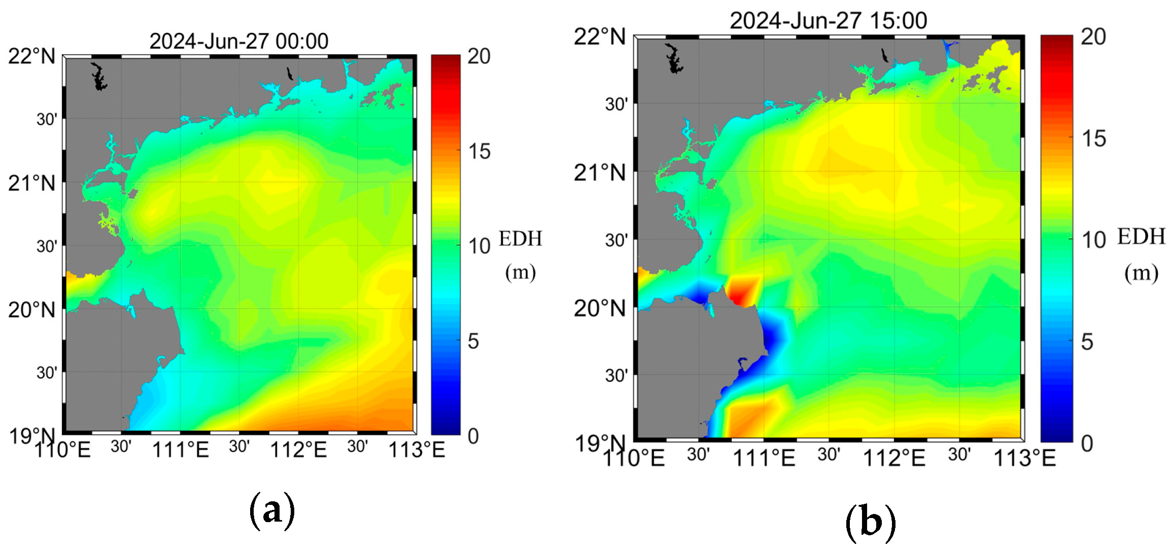
In this paper, we use the meteorological data with spatial and time resolutions of 0.25° × 0.25° and 1 h released at 18 UTC (Coordinated Universal Time) from the GFS to forecast the EDH. As an example, Figure 3 presents the 24 h forecasted EDHs over the northern SCS at 0:00 and 15:00 on 27 June 2024. Note that all time labels in Figure 3 correspond to Beijing Time, i.e., UTC + 8.
Figure 3.
The forecasted EDHs over the SCS at different time on 27 June 2024 (Beijing Time, UTC + 8). (a) 00:00; (b) 15:00.
To further obtain the forecasted EDHs over the maritime OTH communication links with lengths of 150 km, 188 km and 248 km shown in Figure 2a, the GFS grid points closest to each link are selected, and their number is determined by the lengths of the aforementioned OTH links.
Specifically, for the maritime OTH communication link of 150 km (i.e., Jizhao Bay–Wenchang), the coordinates of three selected grid points are (20°25′N, 110°45′E), (20°45′N, 110°45′E) and (21°25′N, 110°45′E), respectively. For the OTH link of 188 km (i.e., Wenchang–Yangxi), the coordinates of the four selected grid points are (20°25′N, 111°00′E), (20°50′N, 111°25′E), (21°00′N, 111°50′E) and (21°50′N, 111°50′E), respectively. For the OTH link of 248 km (i.e., Wenchang–Yangjiang), the coordinates of the five selected grid points are (20°25′N, 111°00′E), (20°50′N, 111°25′E), (20°45′N, 111°25′E), (21°25′N, 111°50′E) and (21°50′N, 111°50′E), respectively. Finally, the mean EDH of the selected grid points is used as the forecasted EDH for each OTH link. As an example, Table 3 shows the forecasted EDHs for the OTH link of 150 km on 25 June 2024.
Table 3.
Forecasted EDHs over the OTH link of Jizhao Bay–Wenchang on 25 June 2024 (m).
It is worth mentioning that the GFS meteorological dataset is available only at integer-hour times, so the forecasted EDHs are also available only at integer-hour times, and the EDHs at half-hour times are approximated by taking the arithmetic mean of the forecasted EDHs at the two adjacent integer-hour time. For example, the EDH at 2:30 is the mean value of EDHs at 2:00 and 3:00.
According to the extensive engineering experience and experimental data, for the maritime OTH communication links of 150 km, 188 km, and 248 km in the northern SCS, the EDH thresholds are 11.8 m, 13.0 m, and 14.0 m, respectively.
The dates shown in Figure 4, Figure 5, Figure 6, Figure 7, Figure 8 and Figure 9 are selected as the representative cases which have complete measured PLs without data interruption caused by severe weather conditions, e.g., strong winds or rainfall. Furthermore, the selected cases cover the ED mechanism, the troposcatter mechanism and the transition states between them, so the performance comparisons between the proposed method and EDHIM can be sufficiently conducted.
Figure 4.
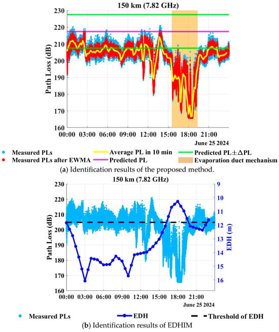
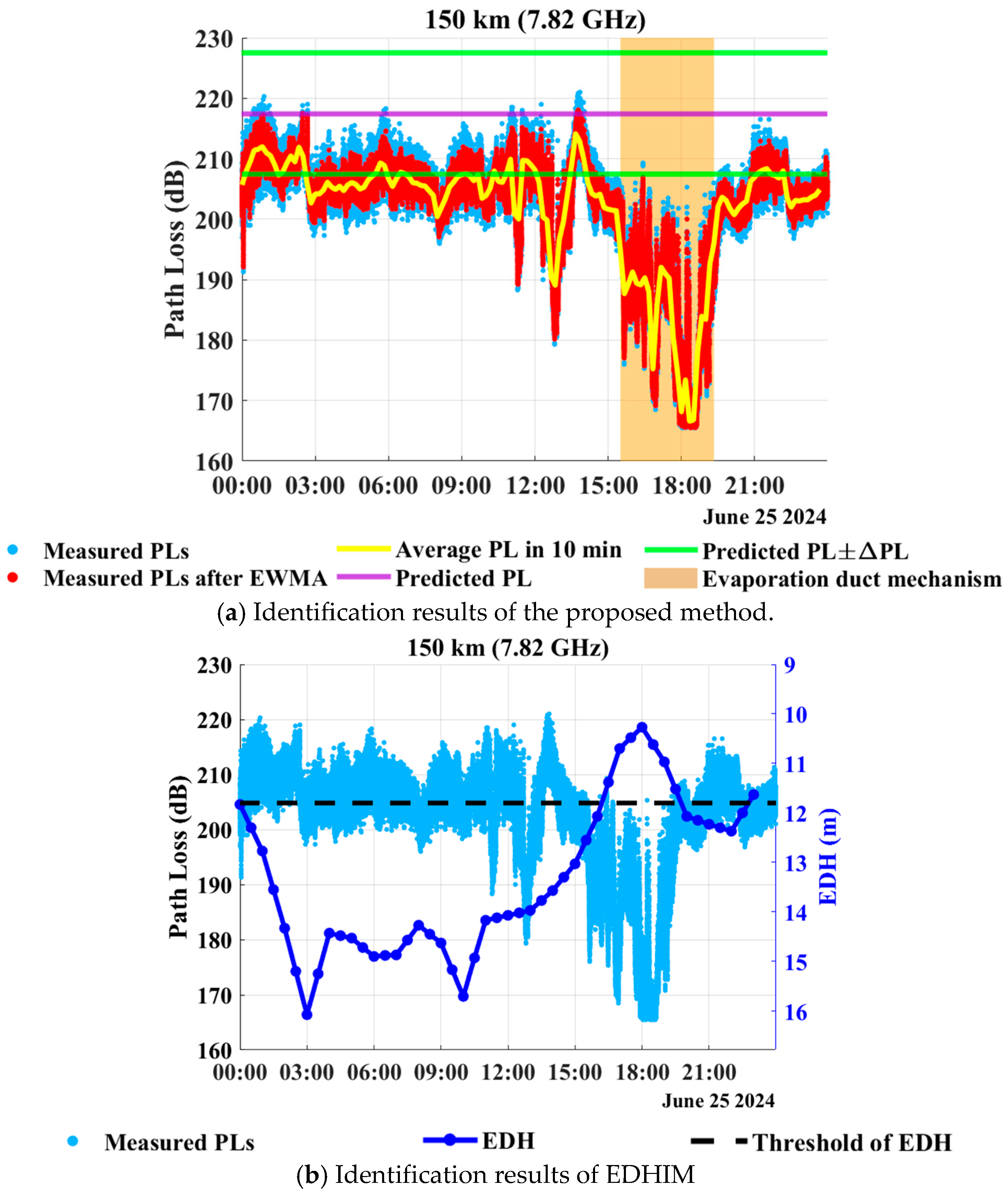
Identification results of maritime OTH propagation mechanisms over the reference link of 150 km on 25 June 2024.
Figure 5.
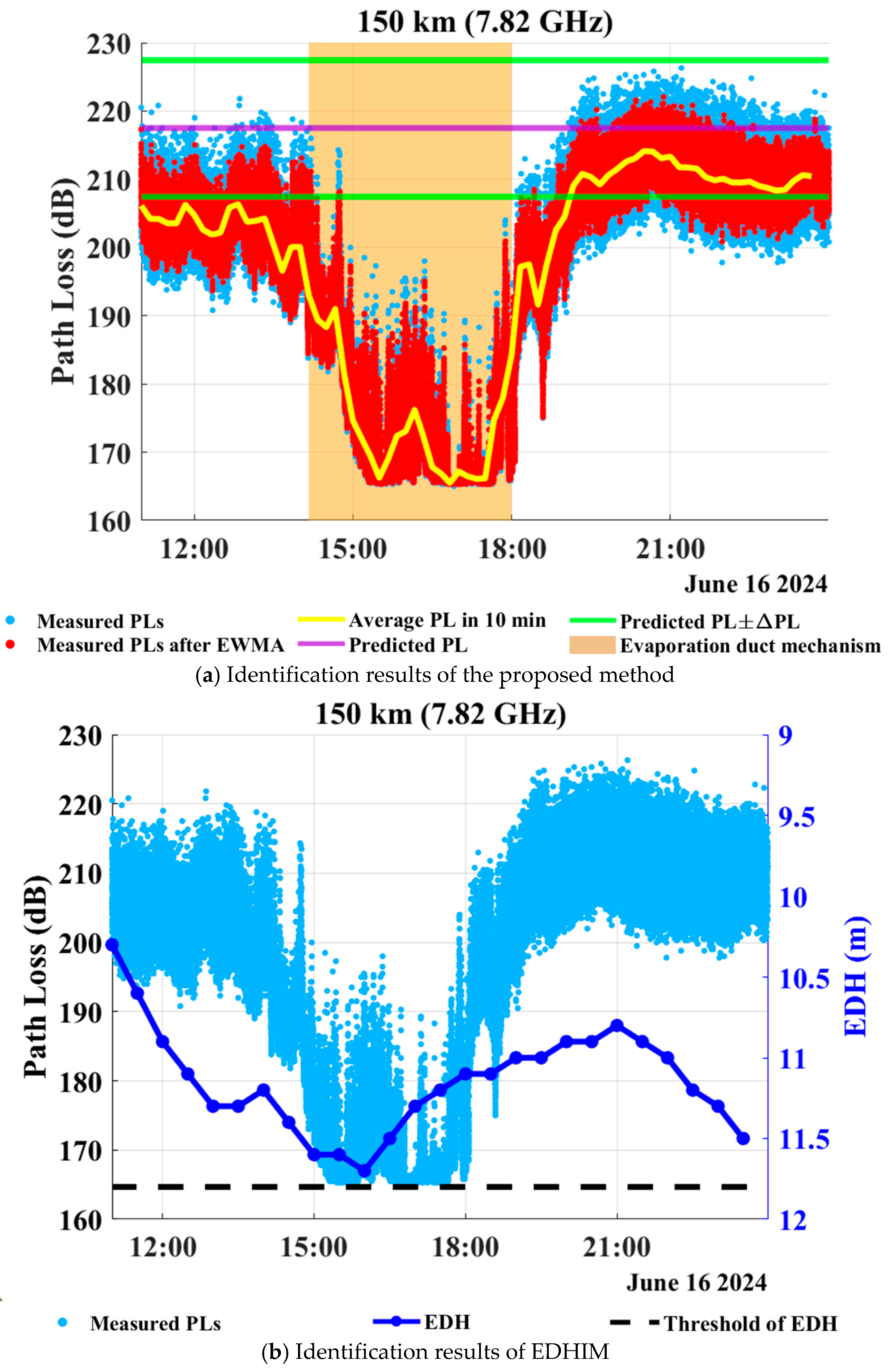
Identification results of maritime OTH propagation mechanisms over the reference link of 150 km on 16 June 2024.
Figure 6.
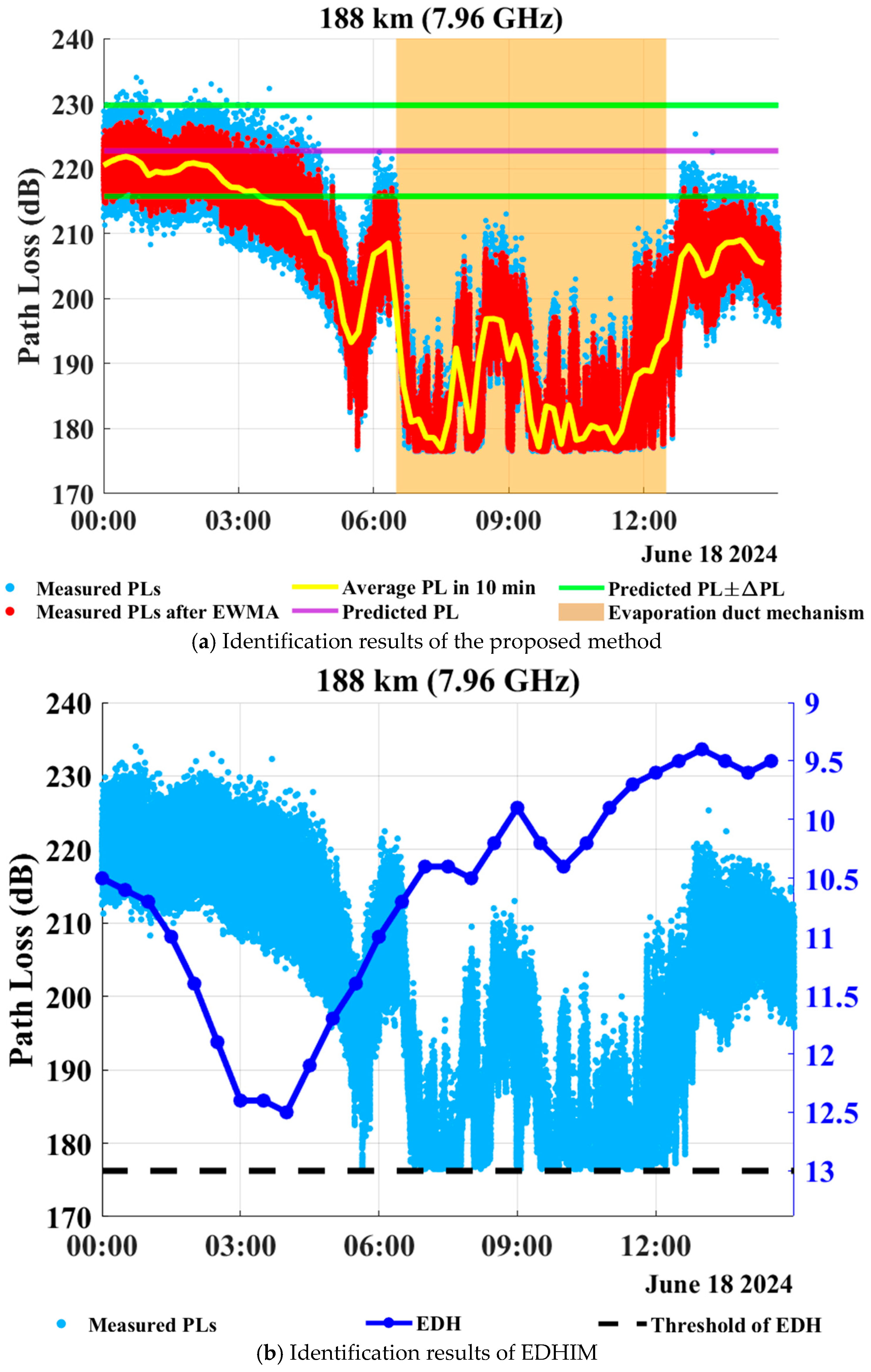
Identification results of maritime OTH propagation mechanisms over the reference link of 188 km on 18 June 2024.
Figure 7.
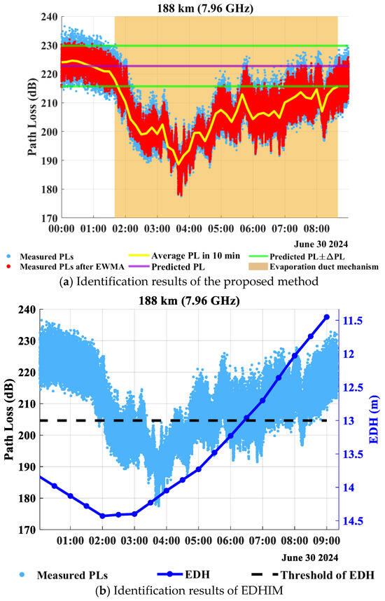
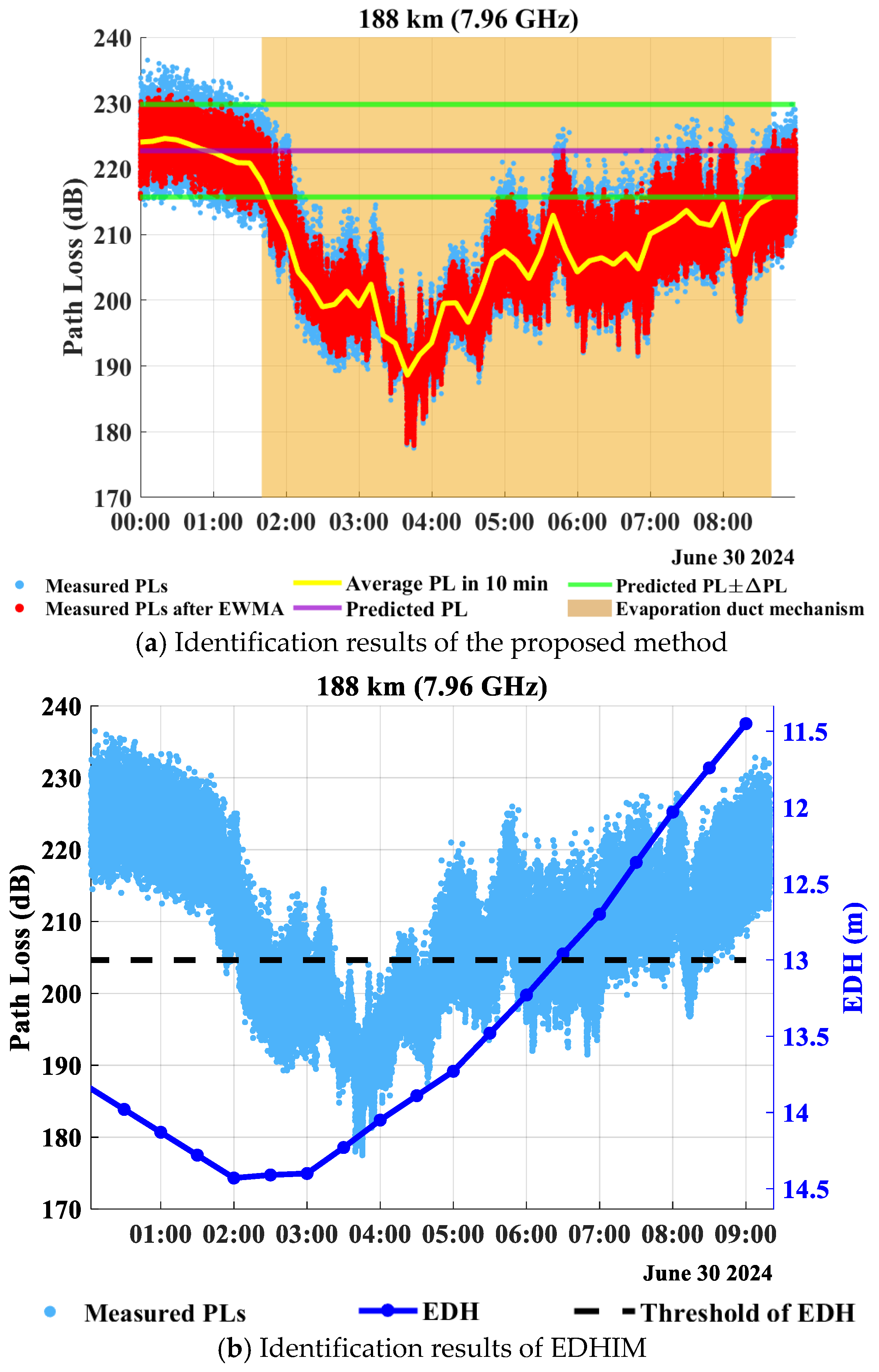
Identification results of maritime OTH propagation mechanisms over the reference link of 188 km on 30 June 2024.
Figure 8.
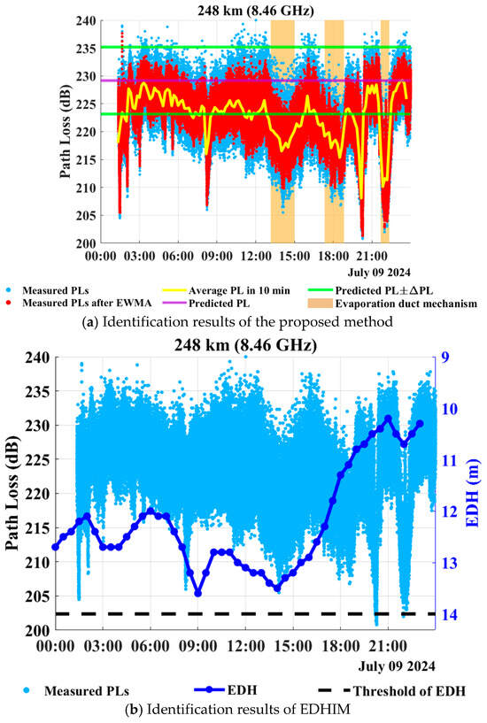
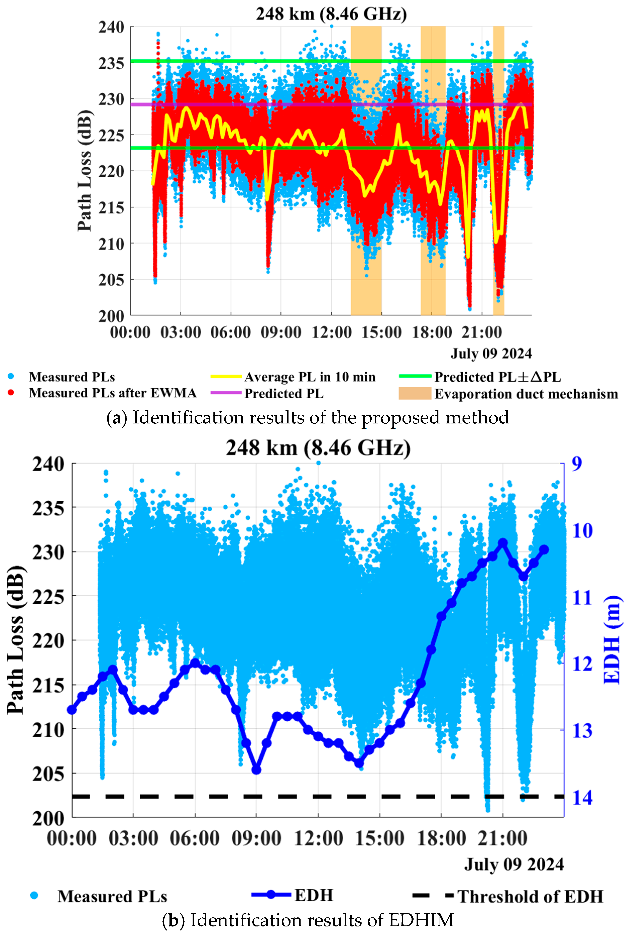
Identification results of maritime OTH propagation mechanisms over the reference link of 248 km on 9 July 2024.
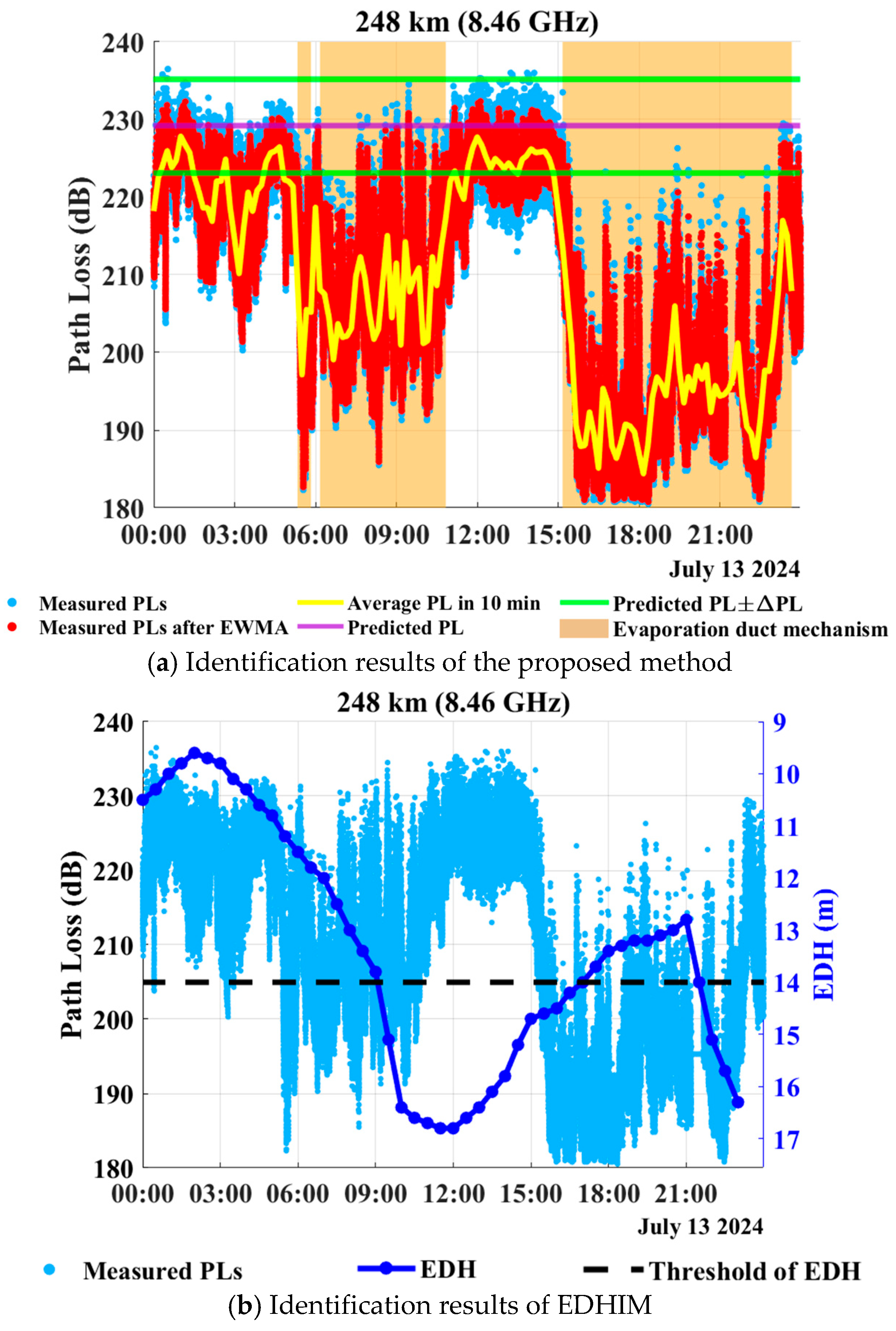
Figure 9.
Identification results of maritime OTH propagation mechanisms over the reference link of 248 km on 13 July 2024.
Figure 4 presents the identification results of the proposed method and EDHIM for the reference link of 150 km (Jizhao Bay–Wenchang) on 25 June 2024, where the operating frequency of the maritime OTH communication system is 7.82 GHz. As shown in Figure 4a, the purple solid line denotes the predicted PL based on the PL prediction model for troposcatter of ITU-R P.617-5. The two green solid lines are derived by adding to and subtracting from this predicted PL, where is the threshold of PL differences between predicted and measured values for reference links of length l1. Therefore, the horizontal strip area bounded by two green solid lines denotes the troposcatter mechanism. During 00:10–02:30 on 25 June, the average PLs in 10 min are located within the horizontal strip area bounded by the two green solid lines, so the proposed method identifies the dominant propagation mechanism as troposcatter. Moreover, as shown in the vertical brown strip area, the interval from 15:30 to 19:20 is identified as one in which an ED is the dominant mechanism, during which time the posterior probability satisfies PED(p) ≥ 0.5. As illustrated in Figure 4b, because the EDH threshold for the reference link of 150 km (i.e., Jizhao Bay–Wenchang) is 11.8 m, and the forecasted EDHs exceed this threshold during 00:10–02:30, so EDHIM identifies an ED as the dominant propagation mechanism.
However, during 00:10–02:30, the time-averaged measured PL is about 210 dB, while the PL predicted by the troposcatter model of ITU-R P.617-5 is about 217 dB. The difference between them is only about 7 dB, which is smaller than the threshold of = 10 dB determined in Section 5.2. According to the identification criterion proposed in (15), the measured PL during this interval is therefore consistent with the propagation characteristics of the troposcatter mechanism. In contrast, EDHIM identifies the dominant mechanism during this interval as an ED, because the forecasted EDH exceeds the threshold of 11.8 m. This discrepancy indicates that identifying the dominant propagation mechanism based on the forecasted EDH may lead to incorrect results in a maritime atmospheric environment.
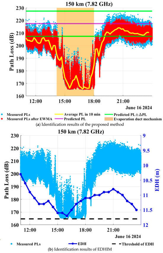
Figure 5 shows the identification results of the proposed method and EDHIM for the reference link of 150 km (Jizhao Bay–Wenchang) on 16 June 2024, where the operating frequency of the maritime OTH communication system is 7.82 GHz. In Figure 5a, during the time interval of 19:00–23:59 on 16 June 2024, the average PLs in 10 min are located within the horizontal strip area bounded by the two green solid lines, so the dominant propagation mechanisms are identified as troposcatter. Moreover, during the interval from 14:10 to 18:00, as shown in the vertical brown strip area, the posterior probability of an ED, i.e., PED(p), satisfies PED(p) ≥ 0.5, indicating that the dominant maritime OTH propagation mechanism is an ED, while the remaining intervals are identified as transition states. Moreover, the identification results of EDHIM are illustrated in Figure 5b. Note that the threshold of EDH for the reference link of 150 km (Jizhao Bay–Wenchang) is 11.8 m. We can observe that the forecasted EDHs on June 16 are lower than the threshold of 11.8 m throughout the day. Therefore, EDHIM identifies the dominant propagation mechanism as troposcatter during the period of 11:00–23:59. However, the time-averaged measured PL during 15:00–18:00 is 171 dB, which is about 40 dB lower than the measured PL during 19:00–21:00, an interval definitely dominated by troposcatter. This indicates that the propagation mechanism during 15:00–18:00 should be an ED. Therefore, during 15:00–18:00, the proposed method provides a more reliable identification than EDHIM.
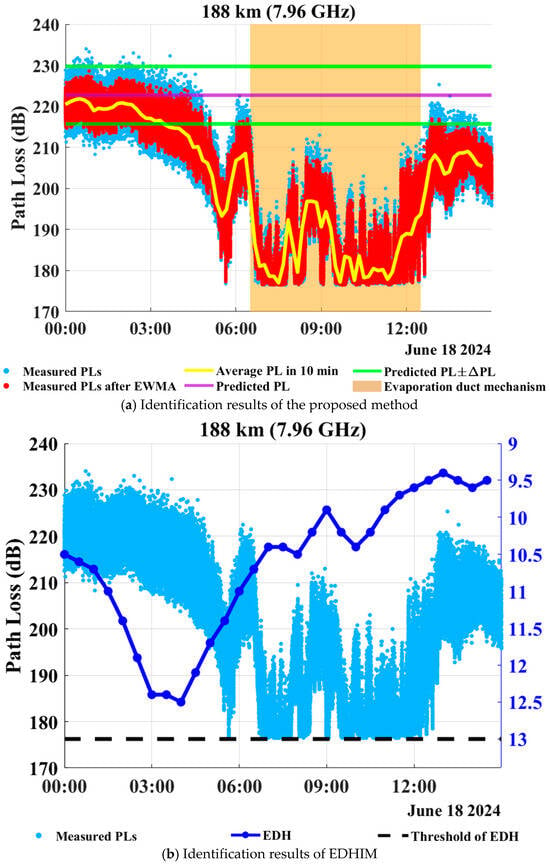
Figure 6 illustrates the identification results for the reference link of 188 km (Wenchang–Yangxi) on 18 June 2024, where the operating frequency of the maritime OTH communication system is 7.96 GHz. In Figure 6a, during 00:00–03:30, the average PLs in 10 min are located within the horizontal strip area bounded by the two green solid lines, so the proposed method identifies the dominant propagation mechanism as troposcatter. Moreover, during the interval of 06:30–12:30, as shown in the two vertical brown strip areas, the dominant propagation mechanisms are identified as EDs, because the posterior probability PED(p) exceeds 0.5. In addition, the interval from 03:30 to 06:30 is identified as a transition state, which indicates that the propagation mechanisms experience a gradual transition from troposcatter to ED. In contrast, as shown in Figure 6b, the EDH threshold of the reference link of 188 km is 13.0 m, and the forecasted EDHs throughout the whole day are lower than 13.0 m, so EDHIM identifies troposcatter as the dominant propagation mechanism during 0:00–15:00. However, during 06:30–12:30, the time-averaged measured PL is only 182 dB, which is about 29 dB lower than the measured PLs during 00:00–03:30. This significant discrepancy indicates that the maritime OTH propagation mechanism during 06:30–12:30 should be an ED rather than troposcatter. Therefore, EDHIM fails to effectively identify the OTH propagation mechanism during 06:30–12:30.
Figure 7 illustrates the identification results for the reference link of 188 km (Wenchang–Yangxi) on 30 June 2024, where the operating frequency of the maritime OTH communication system is 7.96 GHz. In Figure 7a, during 0:00–1:40, the average PLs in 10 min are located within the horizontal strip area bounded by the two green solid lines, so the proposed method identifies the dominant propagation mechanism as troposcatter. Moreover, as illustrated in the two vertical brown strip areas, the intervals 1:40–8:40 are identified as ones in which an ED is the dominant mechanism, because the posterior probability PED(p) exceeds 0.5. In contrast, from Figure 7b we can observe that the forecasted EDHs exceed the threshold of 13.0 m during 0:00–01:40, leading EDHIM to identify the dominant propagation mechanism as an ED. However, the time-averaged measured PL during 0:00–01:40 is 223 dB, which is 23 dB higher than an interval of the ED mechanism. This indicates that the true propagation mechanism during 0:00–01:40 should be troposcatter rather than an ED. As a result, during 0:00–01:40, EDHIM produces a misidentification, whereas the proposed method provides a more reliable identification result.
Figure 8 shows the identification results for the reference link of 248 km (Wenchang–Yangjiang) on 9 July 2024, where the operating frequency of the maritime OTH communication system is 8.46 GHz. In Figure 8a, during 02:10–07:00 and 09:30–11:10, the average PLs in 10 min are located within the horizontal strip area bounded by the two green solid lines, so the dominant propagation mechanism is identified as troposcatter. During 13:10–15:00 and 17:20–18:50, as shown in the two vertical brown strip areas, the posterior probability of an ED, PED(p), exceeds 0.5, so the dominant corresponding mechanism is identified as an ED. Besides, the remaining time intervals are identified as transition states between the two mechanisms. As illustrated in Figure 8b, the EDH threshold for the reference link of 248 km is 14.0 m, and the forecasted EDHs are lower than this threshold throughout the day. Consequently, EDHIM identifies troposcatter as the dominant propagation mechanism for the whole day. Nevertheless, the time-averaged measured PL during 13:10–15:00 is 217 dB, which is 11 dB lower than that during 03:00–05:00. This significant discrepancy indicates that the true propagation mechanism during 13:10–15:00 should be an ED, demonstrating that EDHIM yields a misidentification of the propagation mechanism for this interval.
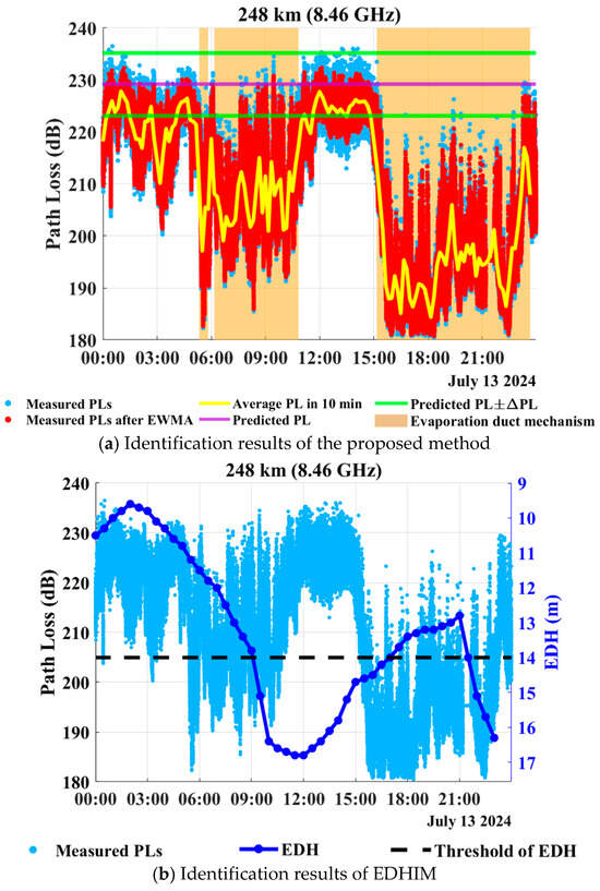
Figure 9 exhibits the identification results for the reference link of 248 km (Wenchang–Yangjiang) on 13 July 2024, where the operating frequency of the maritime OTH communication system is 8.46 GHz. During 00:10–01:30 and 11:30–14:50, the average PLs in 10 min are located within the horizontal strip area bounded by two green solid lines, and thus the dominant propagation mechanism is identified to be troposcatter. In contrast, during 06:10–10:50 and 15:10–23:40, as shown in the two vertical brown strip areas, the posterior probabilities PED(p) exceeds 0.5, indicating the occurrence of an ED. Moreover, as illustrated in Figure 9b, the forecasted EDHs exceed the threshold of 14.0 m during 12:00–15:00, so EDHIM identifies the dominant mechanism as an ED. However, the measured time-averaged PL during 12:00–15:00 is 210 dB, which is only 7 dB lower than that during 03:00–05:00, a time interval obviously dominated by troposcatter. This discrepancy indicates that the true propagation mechanism during 12:00–15:00 should be troposcatter. Consequently, EDHIM fails to effectively identify the propagation mechanism during 12:00–15:00.
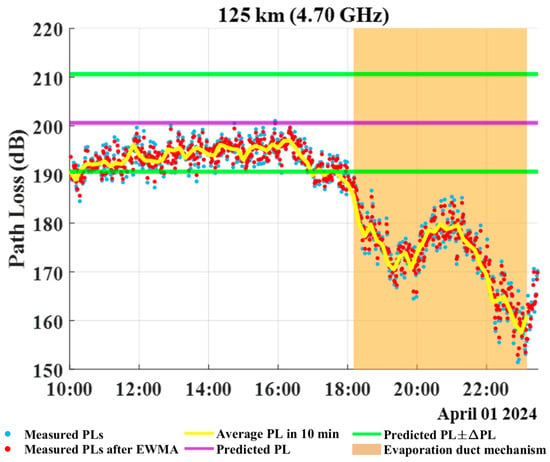
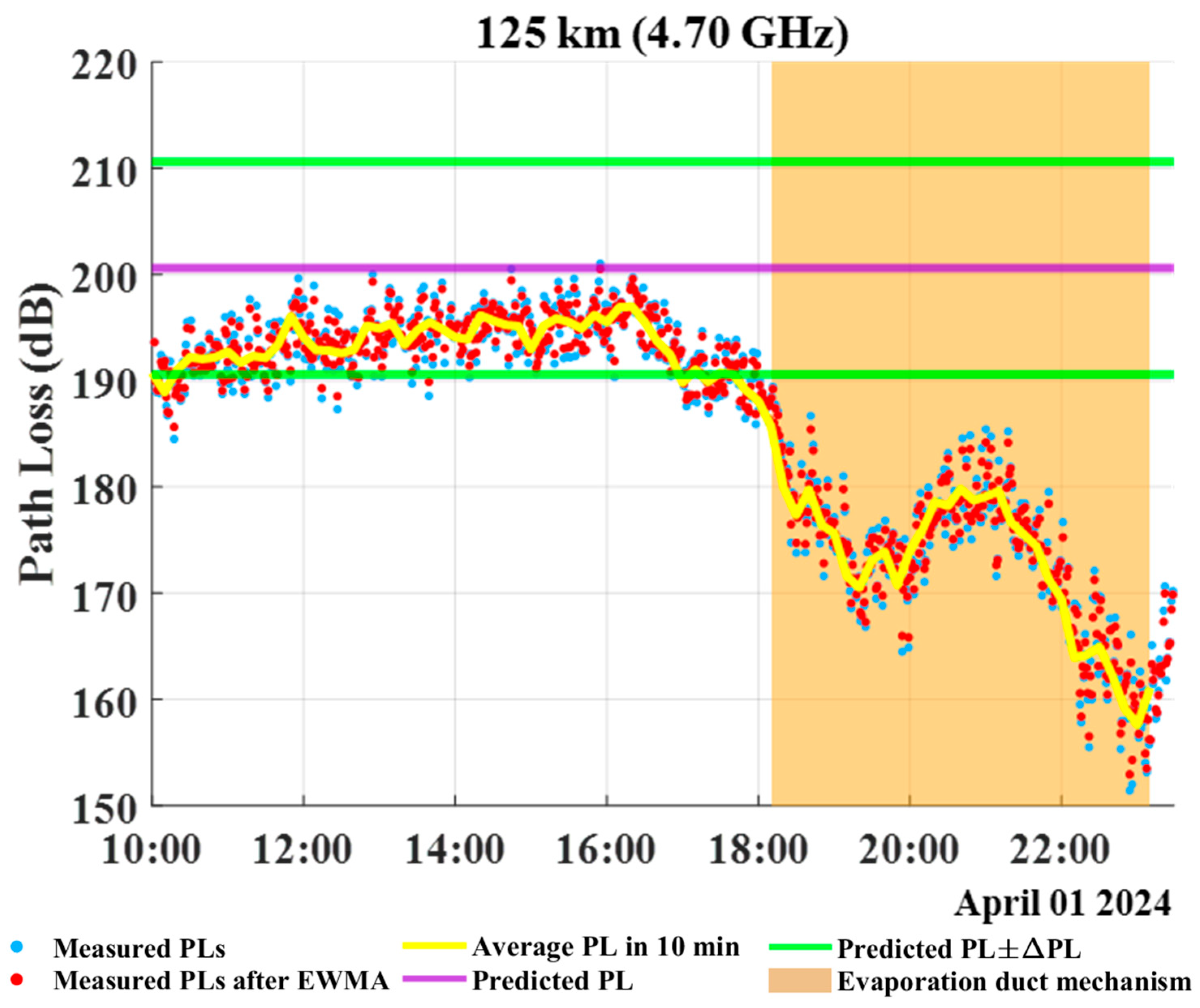
Figure 10 shows the identification results of the proposed method for the constructed OTH link of 125 km in Guangdong Province between Donghai Island (21°01′N, 110°32′E) and Shangyang Town (21°32′N, 110°37′E) on 1 April 2024, where the operating frequency of the maritime OTH communication system is 4.70 GHz. During 10:00–18:00, the average PLs in 10 min are located within the horizontal strip area bounded by the two green solid lines, and thus the dominant propagation mechanism is identified to be troposcatter. After 18:00, as shown in the two vertical brown strip areas, the posterior probabilities PED(p) exceeds 0.5, indicating the occurrence of an ED. The aforementioned results are consistent with the summer cases in Figure 4, Figure 5, Figure 6, Figure 7, Figure 8 and Figure 9, and provide additional validation of the proposed method in spring.
Figure 10.
Identification results of maritime OTH propagation mechanisms over the link of 125 km on 1 April 2024.
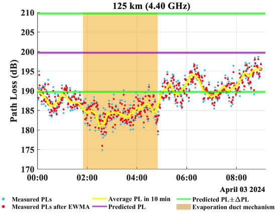
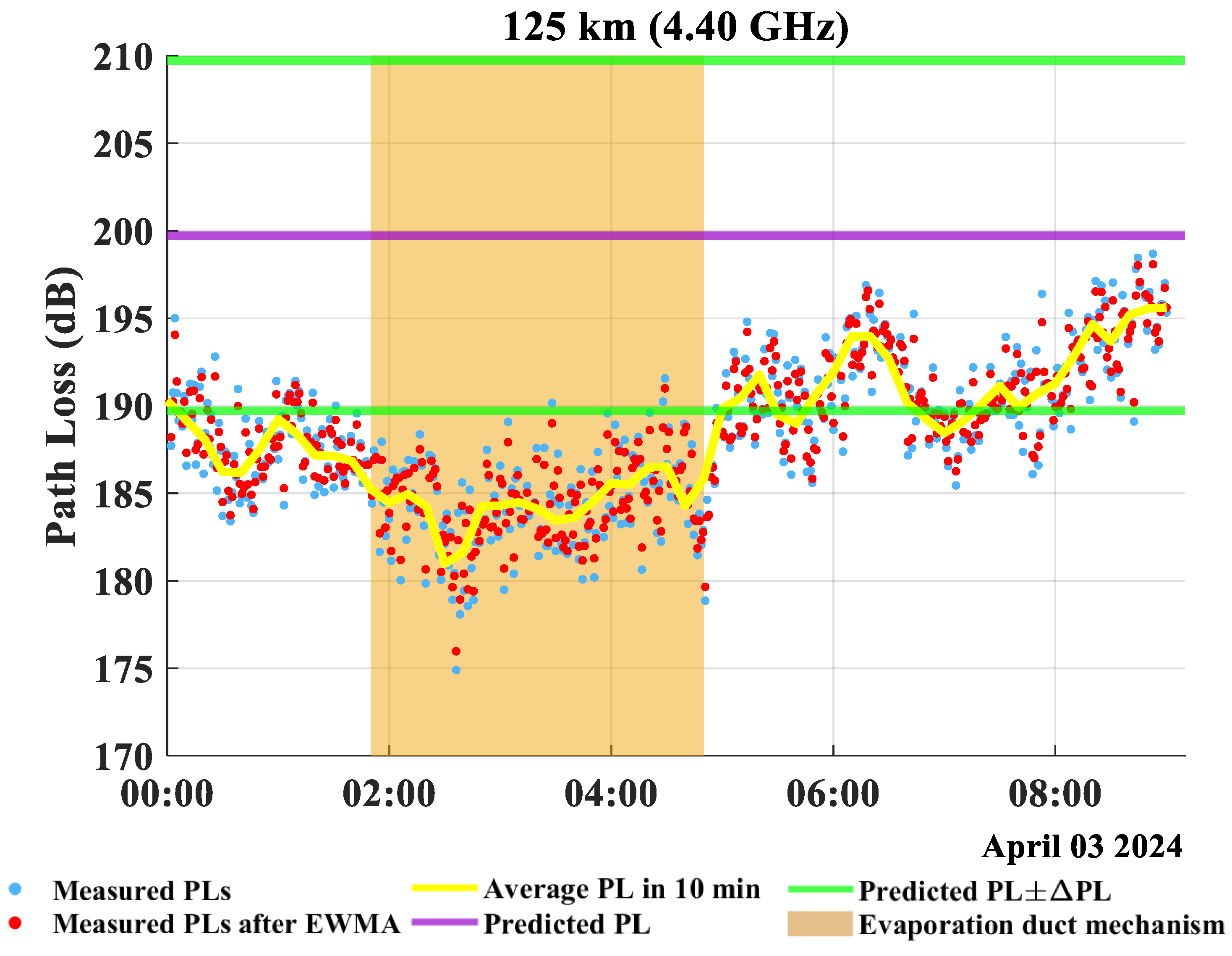
Figure 11 shows the identification results for the same OTH link (Donghai Island-Shangyang Town) on 3 April 2024, where the operating frequency of the maritime OTH communication system is 4.40 GHz. As shown in the two vertical brown strip areas, the posterior probabilities PED(p) exceed 0.5 during 01:50–04:50, indicating the occurrence of an ED, while the transition between the ED and troposcatter is captured during 00:00–01:50. Therefore, the results in Figure 10 and Figure 11 further confirm that the proposed method can identify the dominant OTH propagation mechanism as well as a transition state in spring and C-band.
Figure 11.
Identification results of maritime OTH propagation mechanisms over the link of 125 km on 3 April 2024.
To conclude, the results in Figure 4, Figure 5, Figure 6, Figure 7, Figure 8, Figure 9, Figure 10 and Figure 11 demonstrate that the proposed identification method provides identification results more consistent with the measured PL characteristics than EDHIM under different maritime atmospheric conditions, seasons and frequencies. In particular, the additional spring cases over the maritime OTH link of 125 km (i.e., Donghai Island–Yangxi Town) in Figure 10 and Figure 11 further extend the validation of the proposed identification method to spring and C-band. As a result, the aforementioned results provide technical support for identifying the maritime OTH propagation mechanisms, and thus making the maritime OTH communication systems sufficiently utilize EDs to improve the performance.
5.4. Identification Accuracy Statistics
To quantitatively evaluate the performance of the proposed identification method, the identification results of all time intervals within 10 min from Figure 4, Figure 5, Figure 6, Figure 7, Figure 8 and Figure 9 are aggregated for the statistics of identification accuracy. Currently, there are no existing methods specifically designed for identifying maritime OTH propagation mechanisms from measured PLs. Therefore, identification results obtained via visual inspection as well as physical interpretation are used as the true values of propagation mechanisms. The identification results are statistically analyzed for three categories, i.e., EDs, troposcatter and the transition states between them. In addition, the identification accuracy is defined as the ratio of the number of correctly identified intervals to the total number of intervals.
It is worth noting that EDHIM is only able to identify the ED and troposcatter mechanisms, but cannot directly identify transition states between them, so here we compare the accuracy of the proposed method and EDHIM for identifying the ED and troposcatter mechanisms within a binary identification framework. Furthermore, the identification accuracy of a transition state is solely provided via the three-class confusion matrix of the proposed method. Table 4 presents the three-class confusion matrix of the proposed method, while Table 5 shows the binary confusion matrix of EDHIM. Finally, based on the two confusion matrices, Table 6 further compares the identification accuracy of the proposed method and EDHIM.
Table 4.
The three-class confusion matrix of the proposed identification method.
Table 5.
The binary confusion matrix of EDHIM.
Table 6.
Comparison of identification accuracy.
From Table 6 we know that the identification accuracy of the proposed method for EDs, troposcatter and a transition state is 99.56%, 96.45%, and 69.63%, respectively, and the overall identification accuracy is 86.23%. In contrast, the overall identification accuracy of EDHIM is only 50.86%, with obvious misidentifications of the ED and troposcatter mechanisms. For example, many intervals which are inherently the ED mechanism are misidentified as the troposcatter mechanism, so the identification accuracy of EDs by EDHIM is only 27.73%. More importantly, EDHIM mainly relies on the forecasted EDH and fixed thresholds of EDH; when there exist deviations in the GFS meteorological dataset, it tends to misidentify EDs as troposcatter. Instead, the proposed method directly utilizes the deviations between measured and predicted PLs in the troposcatter mechanism, and then exploits the GMM for unsupervised classification of the remaining intervals, thereby enabling more accurate identification results. Furthermore, the misidentifications of the proposed method primarily occur in the boundary regions of transition states, which is consistent with the physical characteristics of the coexistence and gradual transitions between EDs and troposcatter in practical maritime atmospheric environments.
It is also worth mentioning that in the ED mechanism, the small-scale fading of the received signal envelope obeys the Rician distribution. The reason is that in the ED mechanism, a dominant ED component coexists with the weaker troposcatter component. Therefore, the distribution of the received signal envelope provides an independent criterion for accurately identifying the ED mechanism, and this method does not rely on the forecasted EDH or the proposed identification method. The detailed fitting results and Kolmogorov–Smirnov (KS) test are provided in the Supplementary File.
6. Discussion
The identification accuracy statistics in Table 6 demonstrate that the proposed method achieves an identification accuracy of 99.56%, 96.45% and 69.63% for EDs, troposcatter and transition states, respectively. Finally, the overall identification accuracy of the proposed method is 86.23%, and we treat this result as an indicative, single-dataset evaluation, and acknowledge that validation on independently labeled or external datasets remains an important future step.
Compared with the intuitive identification method EDHIM, whose overall identification accuracy is only 50.86%, the proposed method provides quasi-real-time and more reliable identification of maritime OTH propagation mechanisms. Nevertheless, the identification accuracy of transition states is relatively lower than that of the ED and troposcatter mechanisms, since the misidentifications of the proposed method primarily occur in the boundary regions of transition states, which is consistent with the physical characteristics of the coexistence and gradual transitions between ED and troposcatter in practical maritime atmospheric environments.
It is worth mentioning that, in this paper, the identification results obtained via visual inspection and physical interpretation are used as the true values of the propagation mechanisms, because there are currently no existing methods specifically designed for identifying maritime OTH propagation mechanisms from measured PLs. Therefore, the identification accuracy of the proposed method is evaluated based on the consistency with the variations of measured PLs and physical characteristics of different OTH propagation mechanisms, rather than on predefined mechanism labels. In our future work, we will further compare the proposed method with machine-learning-based identification methods, so as to provide a more comprehensive and quantitative evaluation of the identification performance.
Moreover, the measured PLs used in this paper were obtained from the constructed OTH communication links in the northern SCS. Further validations under more complex maritime atmospheric conditions, other seasons and other sea areas will be conducted in our future work. Specifically, more measured PL data will be obtained from more constructed OTH communication links with different lengths, operating frequencies and antenna heights, so that the thresholds of the difference between the predicted and measured PLs, as well as the parameters of the GMM, can be determined and validated more sufficiently. In addition, the performance of the proposed method under different maritime atmospheric conditions, e.g., severe weather conditions such as strong winds or rainfall, will be further investigated, since the measured PLs in such conditions may contain more abnormal fluctuations. Finally, the proposed identification method can be applied to maritime OTH communication systems to timely and sufficiently exploit ED environments to further improve their performance.
7. Conclusions
In this paper, an identification method of OTH propagation mechanisms has been proposed in maritime atmospheric environments based on measured PLs in the northern SCS. The EWMA method was first exploited to smooth the measured PLs. Then, we proposed an identification criterion as well as a corresponding algorithm to identify the troposcatter mechanism. Subsequently, the GMM combined with the expectation maximization algorithm were utilized to identify the ED mechanism and transition states. Finally, the performance of the proposed method was validated via the measured PLs in X-band obtained from the cross-sea OTH communication experiments in the northern SCS. The results demonstrate that in maritime atmospheric environment, the proposed method provides quasi-real-time and more reliable identification of OTH propagation mechanisms compared with the intuitive identification method EDHIM. Further validations under more complex maritime atmospheric conditions, other seasons and other sea areas will be conducted in our future work. Finally, the proposed identification method can be applied to maritime OTH communication systems to timely and sufficiently exploit ED environments to further improve their performance.
Supplementary Materials
The following supporting information can be downloaded at: https://www.mdpi.com/article/10.3390/rs18213835/s1, Figure S1. PDF fitting for the normalized envelope amplitude under the ED mechanism over the 150 km reference link on 25 June 2024. Figure S2. PDF fitting for the normalized envelope amplitude under the ED mechanism over the 150 km reference link on 16 June 2024. Figure S3. PDF fitting for the normalized envelope amplitude under the ED mechanism over the 188 km reference link on 18 June 2024. Figure S4. PDF fitting for the normalized envelope amplitude under the ED mechanism over the 188 km reference link on 30 June 2024. Figure S5. PDF fitting for the normalized envelope amplitude under the ED mechanism over the 248 km reference link on 9 July 2024. Figure S6. PDF fitting for the normalized envelope amplitude under the ED mechanism over the 248 km reference link on 13 July 2024.
Author Contributions
Conceptualization, H.Z. and T.Y.; methodology, H.Z. and T.Y.; software, T.Y. and W.X.; validation, H.Z., T.Y. and W.X.; formal analysis, T.Y.; investigation, T.Y.; resources, H.Z.; data curation, H.Z.; writing—original draft preparation, T.Y.; writing—review and editing, H.Z.; visualization, X.L.; supervision, K.Y.; project administration, H.Z.; funding acquisition, H.Z. and K.Y. All authors have read and agreed to the published version of the manuscript.
Funding
This work was supported in part by the National Natural Science Foundation of China under Grant 62341133 and 42575063, and in part by the Fundamental and Interdisciplinary Disciplines Breakthrough Plan of the Ministry of Education of China under Grant JYB2025XDXM119.
Data Availability Statement
The measured PL data presented in this paper are available on reasonable request from the corresponding author. The meteorological data used for EDH forecasting were retrieved from the Global Forecast System (GFS) of the National Centers for Environmental Prediction (NCEP), which is publicly accessible at the official website: https://nomads.ncep.noaa.gov/ (accessed between 13 June 2024 and 15 July 2024).
Acknowledgments
We are grateful to the members of the Key Laboratory of Ocean Acoustics and Sensing, Ministry of Industry and Information Technology, for their invaluable assistance in the field experiments and data collection in the northern South China Sea. Special thanks are extended to the academic editor and the anonymous reviewers for their constructive comments and insightful suggestions that have greatly improved the quality of this manuscript. We also acknowledge the National Centers for Environmental Prediction (NCEP) for providing the open-access meteorological datasets used in this paper.
Conflicts of Interest
The authors declare no conflicts of interest.
References
- Lei, X.; Yang, K.; Zhang, T.; Wang, S. Over-the-horizon propagation characteristics of the coupled evaporation duct and tropospheric scatter channels at different frequencies and antenna heights. In Proceedings of the 15th IEEE International Conference on Signal Processing, Communications and Computing (ICSPCC), Hong Kong, China, 18–21 July 2025. [Google Scholar]
- Babin, S.M.; Young, G.S.; Carton, J.A. A new model of the oceanic evaporation duct. J. Appl. Meteorol. 1997, 36, 193–204. [Google Scholar] [CrossRef] [Scilit]
- Yang, C.; Wang, J.; Ma, J. Exploration of X-band communication for maritime applications in the South China Sea. IEEE Antennas Wirel. Propag. Lett. 2022, 21, 481–485. [Google Scholar] [CrossRef] [Scilit]
- Shi, Y.; Zhang, Q.; Wang, S.; Yang, K.; Yang, Y.; Yan, X.; Ma, Y. A comprehensive study on maximum wavelength of electromagnetic propagation in different evaporation ducts. IEEE Access 2019, 7, 82308–82319. [Google Scholar] [CrossRef] [Scilit]
- Huang, L.; Liu, C.; Wang, H.; Zhu, Q.; Zhang, L.; Han, J.; Zhang, Y.; Wang, Q. Experimental analysis of atmospheric ducts and navigation radar over-the-horizon detection. Remote Sens. 2022, 14, 2588. [Google Scholar] [CrossRef] [Scilit]
- Yang, F.; Wang, S.; Yang, K.; Shu, Y.; Shi, Y. Marine high-speed over-the-horizon communications and channel sensing in evaporation ducts over the South China Sea. IEEE Antennas Wirel. Propag. Lett. 2024, 23, 2870–2874. [Google Scholar] [CrossRef] [Scilit]
- Yang, F.; Yang, K.; Shi, Y.; Wang, S.; Zhang, H.; Zhao, Y. The effects of rainfall on over-the-horizon propagation in the evaporation duct over the South China Sea. Remote Sens. 2022, 14, 4787. [Google Scholar] [CrossRef] [Scilit]
- Hu, D.; Yang, K.; Zhang, H.; Wang, S.; Yang, F.; Dong, G.; Shi, Y. Observed diurnal variations of over-the-horizon propagation loss in evaporation duct over the South China Sea. IEEE Antennas Wirel. Propag. Lett. 2024, 23, 1060–1064. [Google Scholar] [CrossRef] [Scilit]
- Xu, W.; Zhang, H.; Yang, K.; Zhang, L.; Yu, T. An improved advanced propagation model considering free-space propagation in evaporation duct environment. IEEE Antennas Wirel. Propag. Lett. 2025, 24, 4730–4734. [Google Scholar] [CrossRef] [Scilit]
- Wang, S.; Yang, K.; Shi, Y.; Yang, F.; Zhang, H.; Ma, Y. Prediction of over-the-horizon electromagnetic wave propagation in evaporation ducts based on the gated recurrent unit network model. IEEE Trans. Antennas Propag. 2023, 71, 3485–3496. [Google Scholar] [CrossRef] [Scilit]
- Dockery, G.D. Modeling electromagnetic-wave propagation in the troposphere using the parabolic equation. IEEE Trans. Antennas Propag. 1988, 36, 1464–1470. [Google Scholar] [CrossRef] [Scilit] [PubMed]
- Li, L.; Wu, Z.; Lin, L.; Zhang, R.; Zhao, Z. Study on the prediction of troposcatter transmission loss. IEEE Trans. Antennas Propag. 2016, 64, 1071–1079. [Google Scholar] [CrossRef] [Scilit]
- Liao, X.; Zhang, Q.; Sun, B.; Zheng, X. Weather forecast-enabled tropospheric scattering path loss modeling for over-the-horizon maritime communications. IEEE Trans. Antennas Propag. 2025, in press. [Google Scholar]
- Yuan, D.; Chen, X. Troposcatter transmission loss prediction based on particle swarm optimisation. IET Microw. Antennas Propag. 2021, 15, 332–341. [Google Scholar] [CrossRef] [Scilit]
- Babin, S.M.; Dockery, G.D. LKB-based evaporation duct model comparison with buoy data. J. Appl. Meteorol. 2002, 41, 434–446. [Google Scholar] [CrossRef] [Scilit]
- Frederickson, P.A.; Davidson, K.L.; Newton, A. An operational bulk evaporation duct model. In Proceedings of the Battlespace ACIMOC, Monterey, CA, USA, 9–11 September 2003. [Google Scholar]
- National Centers for Environmental Prediction. NOAA Operational Model Archive and Distribution System (NOMADS). Available online: https://nomads.ncep.noaa.gov/ (accessed on 26 January 2026).
- Rice, P.L.; Longley, A.G.; Norton, K.A.; Baris, A.P. Transmission Loss Predictions for Tropospheric Communication Circuits; Central Radio Propagation Laboratory, National Bureau of Standards: Boulder, CO, USA, 1965; Volume 2. [Google Scholar]
- Lee, I.-S.; Noh, J.-H.; Oh, S.-J. A survey and analysis on a troposcatter propagation model based on ITU-R recommendations. ICT Express 2023, 9, 507–516. [Google Scholar] [CrossRef] [Scilit]
- International Telecommunication Union. Propagation prediction techniques and data required for the design of trans-horizon radio-relay systems. In ITU-R Recommendation P.617; ITU: Geneva, Switzerland, 2019. [Google Scholar]
- Zhang, M. Troposcatter Propagation; Publishing House of Electronics Industry: Beijing, China, 2004. [Google Scholar]
- Zhao, Q.; Yang, L.; Guo, X.; Zhu, D.; Zhang, Y.; Wei, Y.; Li, Q. Study of the deterministic transmission loss prediction model for troposcatter. IEEE Trans. Antennas Propag. 2023, 71, 6859–6868. [Google Scholar] [CrossRef] [Scilit]
- Hunter, J.S. The exponentially weighted moving average. J. Qual. Technol. 1986, 18, 203–210. [Google Scholar] [CrossRef] [Scilit]
- Kulshrestha, S.; Patel, S. An efficient host overload detection algorithm for cloud data center based on exponential weighted moving average. Int. J. Commun. Syst. 2021, 34, e4708. [Google Scholar] [CrossRef] [Scilit]
- Rasmussen, C.E. The infinite Gaussian mixture model. In Advances in Neural Information Processing Systems; MIT Press: Cambridge, MA, USA, 2000; pp. 554–560. [Google Scholar]
- Yu, D.; Deng, L. Gaussian mixture models. In Automatic Speech Recognition; Springer: London, UK, 2015; pp. 15–34. [Google Scholar]
- Bishop, C.M. Pattern Recognition and Machine Learning; Springer: New York, NY, USA, 2006; pp. 39–40. [Google Scholar]
- Likas, A.; Vlassis, N.; Verbeek, J.J. The global k-means clustering algorithm. Pattern Recognit. 2003, 36, 451–461. [Google Scholar] [CrossRef] [Scilit]
- Moon, T.K. The expectation-maximization algorithm. IEEE Signal Process. Mag. 1996, 13, 47–60. [Google Scholar] [CrossRef] [Scilit]
- Zhao, M.; Edakunni, N.; Pocock, A.; Brown, G. Beyond Fano’s inequality: Bounds on the optimal F-score, BER, and cost-sensitive risk and their implications. J. Mach. Learn. Res. 2013, 14, 1033–1090. [Google Scholar]

Disclaimer/Publisher’s Note: The statements, opinions and data contained in all publications are solely those of the individual author(s) and contributor(s) and not of MDPI and/or the editor(s). MDPI and/or the editor(s) disclaim responsibility for any injury to people or property resulting from any ideas, methods, instructions or products referred to in the content. |
© 2026 by the authors. Licensee MDPI, Basel, Switzerland. This article is an open access article distributed under the terms and conditions of the Creative Commons Attribution (CC BY) license.