


Highlights
What are the main findings?
- WPFM-STF introduces a wavelet-constrained prior-guided Flow Matching framework that formulates remote sensing spatiotemporal fusion as a prior-to-target continuous transport process.
- WPFM-STF maintains competitive reconstruction accuracy while substantially improving inference efficiency, achieving an 8.31–10.91× speedup over the 50-step STFDiff with only a few ODE sampling steps.
What are the implications of the main findings?
- WPFM-STF achieves competitive reconstruction accuracy and spectral consistency with substantially reduced inference cost.
- WPFM-STF provides a favorable accuracy–efficiency trade-off for remote sensing spatiotemporal fusion.
Abstract
Spatiotemporal fusion techniques can generate remote sensing imagery with both high spatial and temporal resolutions, thereby supporting a wide range of Earth observation applications. Although recent diffusion-based STF methods have shown promising reconstruction performance, generation from Gaussian noise typically requires many iterative sampling steps, resulting in considerable inference cost. To enable efficient few-step reconstruction, we propose WPFM-STF, a wavelet-constrained prior-guided Flow Matching framework for remote sensing spatiotemporal fusion, specifically adapting Flow Matching to the characteristics of STF by formulating reconstruction as a continuous transport process from a learned spatiotemporal prior to the target fine-resolution image. Specifically, a learnable prior generator integrates multi-temporal and multi-resolution observations to produce an initial estimate that already captures scene structure and temporal variation, thereby shortening the effective transport path compared with noise-based generation. Conditional Flow Matching is then employed to learn the prior-to-target velocity field, providing a more flexible and progressive refinement process than one-shot regression while enabling accurate reconstruction with only a few ordinary differential equation evaluations. To further preserve fine spatial structures during few-step transport, a wavelet detail constraint is imposed on the high-frequency components of a residual-induced auxiliary reconstruction derived from the predicted velocity field. Extensive experiments on the CIA, LGC, and Daxing datasets demonstrate that WPFM-STF achieves competitive or superior reconstruction performance with only a few ODE evaluations; ablation studies validate the effectiveness of the learned spatiotemporal prior, prior-guided flow refinement, and wavelet detail constraint; and efficiency analyses further confirm its substantial advantage over iterative diffusion-based STF methods.
1. Introduction
Remote sensing spatiotemporal fusion (STF) aims to generate remote sensing imagery with both high spatial and high temporal resolutions by integrating complementary observations acquired from different sensors and dates. Such imagery is essential for a wide range of dynamic Earth observation applications, including land-cover monitoring, crop growth analysis, disaster assessment, and urban expansion observation [1]. However, due to the inherent trade-off among spatial resolution, temporal revisit frequency, and imaging coverage, individual satellite sensors generally cannot simultaneously provide frequent observations and fine spatial details [1,2]. STF therefore provides an effective solution by combining fine-resolution observations at reference dates with temporally frequent coarse-resolution images to reconstruct fine-resolution imagery at target dates [1,3].
Early STF methods mainly relied on hand-crafted assumptions, local similarity relationships, and explicit temporal-change modeling. Representative approaches such as STARFM [3], ESTARFM [4], and FSDAF [5] estimate target-date fine-resolution images by transferring temporal variations observed in coarse-resolution imagery while preserving spatial information from fine-resolution references. These methods provide good interpretability and have been widely used in practical applications. Nevertheless, their performance is often limited in heterogeneous regions or scenes involving abrupt land-cover changes and complex nonlinear temporal dynamics.
With the development of deep learning, CNN-, GAN-, and Transformer-based STF methods have significantly improved nonlinear representation capability by learning complex mappings between multi-source observations and target fine-resolution images [6]. Most existing deep learning approaches perform reconstruction through a direct feed-forward mapping. Although such one-shot prediction is computationally efficient, accurately modeling substantial temporal changes while simultaneously preserving fine spatial structures remains challenging, particularly in regions containing narrow boundaries, small-scale textures, and rapid land-cover variations.
More recently, diffusion models have attracted increasing attention in image generation and restoration because of their stable optimization and progressive refinement capability [7,8]. By progressively transforming Gaussian noise into target images through repeated denoising, diffusion-based methods have achieved promising performance and have been introduced into remote sensing image reconstruction and fusion tasks [9,10]. However, their iterative sampling procedures typically require numerous network evaluations, resulting in considerable inference cost. Although accelerated sampling strategies can reduce the number of denoising steps, aggressive step reduction may degrade reconstruction accuracy and weaken the recovery of high-frequency spatial structures such as field boundaries, road networks, and building edges.
Flow Matching (FM) provides an alternative continuous-time generative modeling framework by learning a velocity field along prescribed probability paths [11]. Recently, FM has been explored in several remote sensing applications. Nonlinear Flow Matching has been introduced for multimodal remote sensing image clustering to model cross-modal transport and feature interactions [12]. For pansharpening, recent approaches have investigated one-step reconstruction using Flow Matching, including residual-learning-based and unbalanced-optimal-transport-guided formulations [13,14]. These studies demonstrate the applicability of FM to remote sensing representation learning and image fusion.
More closely related to spatiotemporal modeling, UniTS [15] develops a unified Flow Matching framework for remote sensing time-series reconstruction, cloud removal, semantic change detection, and forecasting. AGFlow [16] further introduces timestamp-conditioned masked Flow Matching for asynchronous Sentinel-1 SAR and Sentinel-2 optical observations, enabling cloud removal, missing-frame recovery, and reconstruction at user-specified dates. Although these approaches extend FM to remote sensing time-series generation and reconstruction, their primary objectives differ from the classical cross-resolution STF setting considered in this work. In particular, UniTS emphasizes unified modeling across multiple time-series tasks, while AGFlow focuses on temporally asynchronous SAR–optical fusion and missing-data recovery. Neither formulation specifically investigates prior-guided FM refinement using a reference fine-resolution image and bi-temporal coarse-resolution observations for target-date fine-resolution reconstruction. This distinction motivates the investigation of an FM formulation tailored to the observational characteristics of conventional STF.
A key observation of this work is that STF is fundamentally different from unconditional image generation because the target fine-resolution image is already strongly constrained by the available multi-temporal and multi-resolution observations. The reference fine-resolution image provides detailed spatial structures, while the bi-temporal coarse-resolution observations and encode temporal changes from the reference date to the target date. Therefore, initializing reconstruction from an uninformative random state such as Gaussian noise does not fully exploit the task-specific information already contained in the observations. Instead, an informative source state can be constructed before generative refinement.
Based on this observation, we first learn a target-oriented spatiotemporal prior from the available observations. A straightforward way to construct such an estimate is to transfer the coarse-scale temporal difference directly to the reference fine-resolution image. However, the resulting raw estimate may inherit mixed-pixel effects, spatial misalignment, block artifacts, and radiometric discrepancies caused by the resolution gap between coarse- and fine-resolution observations. Therefore, rather than directly using the coarse-difference estimate as the source state, we employ a learnable prior generator to integrate fine-scale spatial structures with target-date temporal information, producing a more reliable and scene-adaptive initialization for subsequent reconstruction.
Given this learned prior, a straightforward strategy is to directly regress the target residual using a single feed-forward network. Such one-shot regression, however, primarily learns an endpoint correction from a fixed source state. From the perspective of the STF task itself, the transformation from a reference-date scene to a target-date scene is often associated with progressive or stage-wise land-surface evolution, such as vegetation growth, phenological changes, water-body dynamics, and gradual land-cover transitions. The continuous-state formulation of Flow Matching is conceptually compatible with such progressive transformations. Although its transport variable should not be interpreted as physical acquisition time, this continuous modeling perspective allows the prior-to-target reconstruction process to be formulated as a continuous state evolution rather than merely a one-shot mapping from a fixed source to an endpoint. More importantly, Flow Matching learns a state- and time-conditioned velocity field over intermediate states along the prior-to-target trajectory. Therefore, its advantage does not arise from additional observational information, but from a richer state-dependent modeling formulation: instead of predicting a single endpoint correction from the fixed prior, it characterizes the remaining prior-to-target transformation over multiple intermediate reconstruction states. During multi-step inference, the required correction can consequently be re-evaluated according to the evolving reconstruction state. Related image-restoration studies have shown that progressive refinement through intermediate states can alleviate the regression-to-the-mean behavior associated with one-shot regression and improve the recovery of realistic image details [17]. This formulation therefore provides a more flexible and progressive refinement mechanism than one-shot regression while retaining efficient ODE-based inference.
Because the learned prior already captures substantial scene-specific spatial and temporal information, the velocity model only needs to model the remaining discrepancy between the prior and the target image. This reduces the difficulty of the prior-to-target transport compared with noise-to-data generation and provides a practical basis for accurate reconstruction with only a few ODE evaluations.
Few-step transport, however, places greater pressure on the preservation of local spatial details. In remote sensing STF, important structures such as field boundaries, road networks, building edges, water-body contours, and local textures are closely associated with high-frequency image components. However, the standard image-domain Flow Matching objective does not explicitly distinguish reconstruction errors across different frequency bands, and localized high-frequency structures may therefore receive insufficient emphasis during few-step refinement. Wavelet decomposition provides a natural multi-scale frequency representation that separates low-frequency approximation components from high-frequency detail components, enabling frequency-selective supervision of fine spatial structures [18]. Motivated by this property, we introduce a wavelet detail constraint to explicitly penalize high-frequency reconstruction errors and improve the preservation of edges, textures, and fine land-cover structures during few-step Flow Matching. The overall motivation of the proposed prior-guided Flow Matching paradigm is illustrated in Figure 1.
Figure 1.
Motivation of the proposed prior-guided Flow Matching paradigm for remote sensing spatiotemporal fusion. (a) Diffusion-based STF methods typically reconstruct the target fine-resolution image from Gaussian noise through iterative denoising, resulting in a relatively long sampling trajectory. (b) The proposed WPFM-STF first constructs a target-oriented spatiotemporal prior and then performs prior-to-target conditional continuous transport, providing an informative initialization for efficient few-step ODE reconstruction.
Based on the above motivation, we propose WPFM-STF, a wavelet-constrained prior-guided Flow Matching framework for remote sensing spatiotemporal fusion. WPFM-STF first constructs a target-oriented spatiotemporal prior by integrating fine spatial structures from the reference fine-resolution observation with temporal-change information from the coarse-resolution observations. The learned prior is then refined through conditional Flow Matching using a dual-stream velocity network that jointly models the evolving transport state and fixed observational conditions. In addition, a wavelet detail constraint is introduced to emphasize high-frequency components during few-step reconstruction and improve the preservation of fine spatial structures.
The main contributions of this work are summarized as follows:
- We introduce Flow Matching into remote sensing spatiotemporal fusion and formulate STF as a continuous prior-to-target transport process, enabling progressive refinement beyond conventional one-shot regression.
- We design a target-oriented spatiotemporal prior generator and a dual-stream conditional velocity network. The prior generator integrates multi-temporal and multi-resolution observations to construct an informative source state, while the velocity network progressively models the remaining prior-to-target transformation for efficient few-step reconstruction.
- We introduce a wavelet detail constraint that explicitly emphasizes high-frequency residual components during few-step Flow Matching, improving the preservation of edges, textures, and fine land-cover structures.
2. Related Work
2.1. Traditional Spatiotemporal Fusion Methods
Early remote sensing spatiotemporal fusion (STF) methods mainly relied on manually designed models and predefined assumptions regarding spatial similarity, temporal consistency, and spectral variation. STARFM [3] estimates target-date fine-resolution images by adaptively weighting neighboring pixels according to spectral similarity, spatial distance, and temporal variation. To improve fusion performance in heterogeneous regions, ESTARFM [4] introduces conversion coefficients to better characterize the relationship between fine- and coarse-resolution observations and alleviate mixed-pixel problems. FSDAF [5] further integrates spectral unmixing, spatial interpolation, and residual compensation to improve reconstruction under complex land-cover changes.
Subsequent traditional STF methods further explored spatial redundancy and temporal relationships among multi-source observations. STNLFFM [19] introduces non-local filtering to exploit spatial self-similarity and temporal correlation among multi-date images. Fit-FC [20] further improves temporally dense fine-resolution image reconstruction by introducing a three-stage framework consisting of regression model fitting, spatial filtering, and residual compensation. Although these methods provide strong physical interpretability and do not require large-scale training datasets, their performance largely depends on manually designed assumptions and predefined transformation models. Consequently, they may struggle with nonlinear temporal variations, abrupt land-cover changes, and complex spatial heterogeneity commonly observed in real remote sensing scenarios. These limitations motivate the development of data-driven approaches with stronger representation capability.
2.2. Deep Learning-Based Spatiotemporal Fusion Methods
With the rapid development of deep learning, STF methods have gradually shifted from handcrafted models toward data-driven representation learning. Deep neural networks can automatically extract nonlinear spatial and temporal representations from multi-source observations and learn complex mappings between input images and target fine-resolution images.
CNN-based methods first introduced convolutional architectures into STF. DCSTFN [21] employs deep convolutional networks to learn nonlinear transformations between multi-temporal observations, demonstrating the effectiveness of deep feature extraction for STF tasks. EDCSTFN [22] further improves feature representation through an enhanced encoder–decoder architecture and achieves better reconstruction performance. However, CNN-based methods mainly rely on local receptive fields, which may limit their capability to capture long-range spatial dependencies.
To improve perceptual reconstruction quality, GAN-based methods introduce adversarial learning into STF. GANSTFM [23] adopts a conditional generative adversarial framework to generate visually realistic fusion results. Although adversarial learning can enhance texture reconstruction, it may also introduce spectral distortion when generated details are insufficiently constrained.
Recently, attention mechanisms and Transformer architectures have been explored to improve global dependency modeling. ECPW-STFN [24] introduces wavelet transform into spatiotemporal fusion to separately model low- and high-frequency components and employs a compound loss to improve detail preservation. SwinSTFM [25] employs shifted-window attention to capture long-range spatial interactions and improve reconstruction in complex scenes. FSDFormer [26] further introduces frequency-domain and spatial-domain feature learning to enhance the representation of spatial details and spectral information in spatiotemporal fusion tasks. Related advances in remote sensing image restoration have also emphasized joint spatial–spectral modeling. For example, MSG-Former [27] employs multi-scale spatial–spectral feature learning for hyperspectral image denoising, offering a complementary perspective on spatial detail preservation and spectral representation. More recently, state-space models have been introduced into STF. Mamba-STFM [28] explores the Mamba architecture for efficient long-range dependency modeling, while STFMamba [29] further investigates visual state-space models for remote sensing image fusion.
Despite these advances, most existing deep learning-based STF methods reconstruct the target fine-resolution image through a single feed-forward mapping. Although such deterministic reconstruction strategies are computationally efficient, a one-shot prediction may have limited flexibility in progressively correcting residual spatial and spectral discrepancies, particularly under complex temporal variations. This motivates the exploration of iterative and continuous refinement formulations that can decompose the reconstruction process into a sequence of intermediate transformations.
2.3. Generative Models for Spatiotemporal Fusion
Generative models have recently provided new perspectives for remote sensing image reconstruction by learning complex image distributions beyond deterministic regression. Diffusion models have achieved remarkable success in image generation and restoration by constructing gradual transitions from noise distributions to target data distributions.
DDPM [7] formulates generation as an iterative reverse denoising process, where clean samples are progressively recovered from Gaussian noise. DDIM [8] accelerates diffusion sampling by introducing a non-Markovian formulation while maintaining competitive generation quality. Score-based generative models further interpret diffusion generation through score estimation and stochastic differential equations [30]. Latent diffusion models [31] improve computational efficiency by performing diffusion in a compressed latent space. Consistency models [32] further explore one-step and few-step generation by learning consistent mappings between different noise levels.
Diffusion-based approaches have also been introduced into remote sensing image reconstruction and fusion tasks. DDRF [9] incorporates conditional diffusion modeling into remote sensing image fusion by introducing auxiliary information into the denoising process. SSDiff [10] integrates spatial and spectral information into a diffusion framework for remote sensing pansharpening. For remote sensing spatiotemporal fusion, STFDiff [33] introduces a diffusion-based generation framework to predict target-date fine-resolution images from multi-source observations.
Although diffusion-based methods benefit from strong distribution modeling capability, they generally follow a noise-to-target generation paradigm. Starting from Gaussian noise requires iterative sampling procedures, leading to considerable inference costs. Recent studies, including EDM [34] and DPM-Solver [35], have investigated efficient diffusion sampling strategies to reduce computational complexity. However, for strongly conditioned reconstruction tasks such as STF, the available observations already contain substantial spatial and temporal information that can potentially be exploited to construct a more informative generation trajectory.
Flow-based generative models provide an alternative perspective by formulating generation as a continuous transport process between source and target distributions. Neural ODEs [36] describe generation through continuous-time dynamical systems, while Flow Matching [11] directly learns a time-dependent vector field that transports samples along predefined probability paths. Conditional Flow Matching [37] further extends this framework by introducing conditional transport objectives. Rectified Flow [38] improves transport efficiency by encouraging straighter trajectories, while scalable architectures such as SiT [39] further demonstrate the potential of flow-based models for efficient image generation.
Recent image restoration studies have further explored task-specific generation trajectories that make explicit use of degraded observations or intermediate estimates. ResShift [40] constructs a residual-shifting diffusion process between low- and high-resolution images, replacing the conventional direct noise-to-image transition with a restoration-oriented trajectory. PMRF [41] first predicts a posterior-mean estimate and subsequently transports it toward the high-quality image distribution using Rectified Flow. ResFlow [42] models image degradation as a deterministic continuous flow and performs restoration by reversing the learned degradation process. Collectively, these studies suggest that incorporating task-specific observations or intermediate estimates into the generative trajectory can provide more informative starting states for image restoration.
Nevertheless, these approaches are primarily designed for general image restoration tasks and do not explicitly exploit the multi-temporal and multi-resolution observation structure of remote sensing STF. In STF, the reference fine-resolution image provides detailed spatial information, while multi-temporal coarse-resolution observations encode temporal changes related to the target date. Motivated by this characteristic, we construct a target-oriented spatiotemporal prior from the available observations and use it as the source state of the conditional flow-matching process. In this manner, the subsequent flow focuses on modeling the transformation from an informative task-specific prior toward the target fine-resolution image, providing a practical basis for efficient few-step reconstruction.
2.4. Frequency-Aware Reconstruction
High-frequency spatial information plays an essential role in remote sensing image reconstruction because object boundaries, road networks, farmland edges, and fine textures are mainly characterized by local high-frequency variations. Conventional pixel-wise reconstruction losses optimize intensity-level consistency in the spatial domain but do not explicitly distinguish errors across different frequency components. Consequently, models trained only with spatial-domain objectives may produce over-smoothed predictions and insufficiently recover fine structures, especially under few-step generative processes.
Wavelet decomposition provides a natural multi-scale representation by separating images into low-frequency approximation components and high-frequency detail components. Mallat [43] established the theoretical foundation of wavelet representation, while Daubechies [44] further developed wavelet analysis.
Recent studies have demonstrated the effectiveness of frequency-aware objectives for image restoration and generation. Guided Frequency Loss [45] combines spatial-domain reconstruction objectives with frequency-domain supervision to improve detail recovery. Focal Frequency Loss [46] emphasizes difficult-to-reconstruct frequency components for image reconstruction and synthesis. WaveDM [47] further demonstrates that wavelet-based modeling of low- and high-frequency components can improve structural detail preservation in diffusion-based restoration. Moreover, wavelet-domain losses [18] have shown that explicitly constraining high-frequency wavelet subbands improves reconstruction accuracy and perceptual quality.
However, existing frequency-aware methods mainly focus on deterministic restoration or diffusion-based generation. How to preserve high-frequency spatial structures during efficient few-step flow-based STF reconstruction remains insufficiently explored. Since few-step generation requires accurate reconstruction within a limited number of transport steps, additional frequency-aware supervision is necessary to alleviate detail degradation. Motivated by these observations, WPFM-STF introduces a wavelet detail constraint into the Flow Matching objective to provide frequency-specific supervision beyond conventional spatial-domain reconstruction.
3. Method
3.1. Overall Framework
Given a reference fine-resolution image acquired at time , a coarse-resolution image acquired at the same time, and a coarse-resolution image acquired at the target time , remote sensing spatiotemporal fusion aims to reconstruct the target fine-resolution image .
For notation consistency, let B denote the number of spectral bands, and let H and W denote the height and width of the fine-resolution images, respectively. The reference and target fine-resolution images are represented as
The original coarse-resolution observations are represented as
where and denote the coarse spatial dimensions. After spatial alignment and upsampling, the coarse-resolution observations are mapped to the fine-resolution grid. Unless otherwise specified, the batch dimension is omitted throughout the theoretical formulation for clarity. Unlike diffusion-based methods that start generation from Gaussian noise and recover the target image through iterative denoising, the proposed WPFM-STF introduces a prior-to-target generation paradigm. Specifically, WPFM-STF first learns a target-oriented spatiotemporal prior from multi-source observations and then models the continuous transformation from this informative prior state to the target fine-resolution image through the Flow Matching framework. The overall framework is illustrated in Figure 2.
Figure 2.
Overall framework of the proposed WPFM-STF. (a) Prior-to-target generation pipeline. (b) Target-oriented spatiotemporal prior generator. (c) Prior-guided Flow Matching with wavelet detail constraint and few-step ODE sampling.
The proposed framework follows a two-stage prior-to-target generation strategy consisting of target-oriented prior construction and flow-based target reconstruction. A wavelet detail constraint is further introduced as auxiliary supervision during training to emphasize high-frequency reconstruction errors under few-step generation.
In the first stage, the target-oriented spatiotemporal prior generator takes , , and as inputs and produces a learned prior
By jointly exploiting spatial structures from the reference fine-resolution observation and temporal-change information from the bi-temporal coarse-resolution observations, the generated prior provides an informative initialization related to the target state. Unlike the random-noise initialization commonly adopted in generative models, P already contains scene-specific spatial and temporal information, allowing the subsequent flow model to focus on the remaining prior-to-target correction.
In the second stage, the prior-guided Flow Matching module treats P as the source state and learns a conditional continuous transport trajectory from P to the target image . During training, intermediate states are constructed along the prior-to-target path, and the velocity network is optimized to predict the corresponding target velocity. During inference, the learned velocity field is integrated from using a few-step numerical ODE solver to obtain
where denotes the conditional velocity network and denotes the available conditional observations.
To preserve high-frequency spatial details during few-step generation, we introduce a wavelet detail constraint during training. Given the predicted velocity , an image-domain estimate is constructed as
A one-level Haar discrete wavelet transform (DWT) is then applied to and , and their high-frequency coefficients are explicitly constrained. The detailed loss formulation is presented in the loss-function section.
The complete training and inference procedures of WPFM-STF are summarized in Algorithm 1. The prior generator is first pretrained and frozen, after which the conditional velocity network is trained along the prior-to-target interpolation path. During inference, the learned prior is used as the initial ODE state and progressively updated using a few Euler steps.
| Algorithm 1 Training and inference procedure of WPFM-STF. |
| Input: Training samples , prior generator , velocity network , and number of ODE steps K. |
| Stage I: Target-oriented prior learning |
| 1. Generate the target-oriented prior: . |
| 2. Optimize using , and then freeze . |
| Stage II: Prior-guided Flow Matching |
| 3. Sample and construct the interpolation state: . |
| 4. Define the target velocity: . |
| 5. Predict the conditional velocity: . |
| 6. Construct the auxiliary target estimate: . |
| 7. Optimize using . |
| Inference |
| 8. Initialize the ODE state: . |
| 9. for do |
| , |
| . |
| 10. end for |
| Output: . |
The following subsections describe the target-oriented prior generator, the prior-guided Flow Matching formulation, and the associated loss functions in detail.
3.2. Spatiotemporal Prior Generator
In the proposed prior-guided Flow Matching framework, the quality of the source state affects the magnitude and complexity of the subsequent prior-to-target transformation. Therefore, instead of starting from an uninformative source state, we construct a target-oriented spatiotemporal prior by exploiting the fine-resolution spatial information in and the temporal-change information contained in the coarse-resolution observations.
As illustrated in Figure 3, the prior generator consists of a temporal cue constructor, a fine spatial encoder, a temporal-change encoder, and a residual decoder.
Figure 3.
Detailed architecture of the proposed spatiotemporal prior generator. The module extracts spatial information from and temporal-change cues from the coarse-resolution observations to estimate a residual correction , which is combined with to construct the target-oriented prior P for subsequent flow transport.
The coarse-resolution observations are first resized to the fine-resolution grid:
where denotes bilinear upsampling and
The coarse-scale temporal variation is then computed as
Following the temporal-difference assumption commonly adopted in spatiotemporal fusion, a raw coarse-difference prior is further constructed as
Although provides a direct approximation of target-date changes, it may inherit spatial inconsistencies and coarse-resolution artifacts from the upsampled temporal difference. Therefore, is used as an auxiliary temporal cue rather than directly serving as the final source state.
The fine spatial encoder preserves the structural information contained in the reference fine-resolution image:
where denotes the fine spatial encoder. Let K denote the number of latent feature channels. The spatial representation is written as
Meanwhile, the temporal-change encoder receives the concatenation of the upsampled coarse observations, the reference fine-resolution image, the explicit temporal difference, and the raw coarse-difference prior:
Since each input contains B spectral channels,
The corresponding temporal-change feature is obtained as
where denotes the temporal-change encoder.
Both and are implemented using CNN encoders. Each encoder contains an initial convolution, a SiLU activation, and three residual blocks. Their outputs have the same spatial and channel dimensions and are fused by element-wise addition:
The fused representation is then passed through the prior residual decoder to predict a bounded image-domain residual:
A final convolution in maps the latent K-channel representation back to the B spectral channels.
Instead of directly predicting the target image, the prior generator adopts a residual formulation:
where s denotes a fixed residual scaling factor. In our implementation, is used to control the magnitude of the prior correction.
This formulation preserves reliable spatial information from while introducing target-date variations inferred from the coarse observations. Consequently, the learned prior provides an informative source state for the subsequent prior-guided Flow Matching process.
3.3. Prior-Guided Flow Matching
Flow Matching models the transformation from a source state to a target state as a continuous-time transport process. Let denote the source state and denote the target state. The intermediate state at an artificial transport variable is defined by a prescribed transport path
where satisfies
A commonly adopted choice is the linear interpolation path
The target velocity field associated with the prescribed trajectory is defined as the instantaneous variation of the state:
For the linear path above, the target velocity becomes
Rather than numerically solving the transport ODE during training, Flow Matching trains a neural velocity field to approximate the target velocity at randomly sampled intermediate states:
where c denotes the available conditional observations. Conceptually, the Flow Matching objective minimizes the discrepancy between the predicted and target velocities:
After training, the learned velocity field defines the ordinary differential equation
whose numerical integration transports the source state toward the target state .
In generative applications, the source state is commonly sampled from a simple reference distribution such as Gaussian noise. Remote sensing spatiotemporal fusion, however, is a strongly conditioned reconstruction task. The observations , , and already contain substantial spatial and temporal information related to the unknown target image . Starting the transport from an uninformative random state therefore does not fully exploit the available STF observations. To address this issue, WPFM-STF uses the learned target-oriented spatiotemporal prior P as the source state and formulates reconstruction as a continuous prior-to-target transport process.
Specifically, in WPFM-STF, the source and target states are defined as
where
Accordingly, the linear transport path becomes
and differentiating this path with respect to t gives the target conditional velocity
Thus, for each prior-target pair, the prescribed trajectory is a straight path from the learned prior P to the target image , while the target velocity represents the residual displacement required to transform the prior into the target. Compared with a random source state, the learned prior provides an informative STF-specific starting point, allowing the subsequent Flow Matching stage to focus on the remaining prior-to-target correction.
Given an intermediate state , the conditional velocity network predicts
where
Here, t is an artificial transport variable that indicates the position of the current state along the reconstruction trajectory and should not be confused with the physical acquisition times and .
The conditional velocity network is designed to determine the remaining correction required at each transport state according to the current image state, the transport variable, and the available STF observations. As shown in Figure 4, it consists of a condition encoder , a time-conditioned state encoder , and a residual velocity decoder .
Figure 4.
Architecture of the conditional velocity prediction network . (a) Overall conditional velocity prediction network. (b) Conditional encoder and time-conditioned state encoder. (c) Residual velocity decoder. (d) Basic network blocks.
The condition encoder extracts multi-scale representations from , , and . Its role is to provide observation-dependent spatial and temporal guidance for the velocity prediction. In contrast, the state encoder processes the current intermediate state and characterizes the reconstruction state reached at the current transport step. Separating these two information sources allows the network to explicitly compare the current transport state with the observation-derived guidance.
Because the intermediate state varies continuously along the prior-to-target transport trajectory, the velocity network is conditioned on the scalar time variable t to distinguish different transport stages. Specifically, t is encoded using a sinusoidal embedding followed by a multilayer perceptron. The resulting time representation is injected into the state features through scale-and-shift modulation:
where and are time-dependent modulation parameters generated from the time embedding. This mechanism allows the network to adapt its intermediate representation according to the current location along the prior-to-target path.
At the i-th resolution level, the two encoder branches produce dimensionally aligned features
where , , and denote the channel number and spatial dimensions at that feature level. Here, denotes the encoded feature of the current flow state , while denotes the corresponding feature extracted from the conditional branch. Their discrepancy is explicitly represented as
The residual feature represents the multi-scale feature deviation of the current state relative to the condition-derived reference. Since the velocity field is required to estimate the remaining transformation from the current state toward the target, this explicit discrepancy representation allows the decoder to focus on the information that still needs to be corrected. By computing at multiple resolutions, the network can capture both large-scale structural deviations and fine-scale local differences.
The residual velocity decoder progressively aggregates , , and from coarse to fine resolutions. Coarse-scale features capture large-scale structural discrepancies, whereas finer-scale features provide localized spatial corrections. The decoder finally maps the aggregated residual representation back to the image domain to obtain
During inference, the target image is unavailable. The pretrained prior generator first produces
and the transport process is initialized as
The reconstructed image is then obtained by numerically integrating the learned conditional velocity field:
At each integration step, the velocity field is reevaluated according to the current state , the transport variable t, and the conditional observations c. After integration from to , the final state is taken as the reconstructed fine-resolution image:
3.4. Loss Function
The proposed WPFM-STF is optimized in two stages. In the first stage, the spatiotemporal prior generator is independently pretrained under the supervision of the target fine-resolution image . The prior pretraining objective combines the loss and mean squared error (MSE):
where
and N denotes the total number of elements in the predicted prior. The weighting coefficients are set to and . After pretraining, the parameters of the prior generator are frozen during the subsequent Flow Matching stage.
In the second stage, the learned prior P is treated as a fixed source state. Given a paired prior-target sample , a transport variable is randomly sampled, and the intermediate state along the prescribed linear prior-to-target path is constructed as
The corresponding target conditional velocity is
The velocity network receives the intermediate state , the transport variable t, and the conditional observations , and predicts the corresponding velocity field. The Flow Matching objective is defined as
This objective directly constrains the predicted velocity toward the prior-to-target displacement . However, the image-domain loss does not explicitly distinguish reconstruction errors according to their frequency or orientation. In remote sensing imagery, fine structures such as field boundaries, road networks, building edges, water-body contours, and local textures are closely associated with localized high-frequency variations. Motivated by previous studies showing that wavelet-domain supervision can improve the recovery of fine-scale structures [18], we introduce a Haar-wavelet detail constraint to provide frequency- and orientation-selective regularization of the Flow Matching residual.
For a local image patch
the three high-frequency Haar detail coefficients used in this work are computed as
These coefficients are obtained from the separable Haar low-pass and high-pass filters
The , , and subbands respond to directional local intensity variations and discontinuities and are therefore sensitive to edges, textures, and fine structural transitions, whereas the low-frequency subband mainly represents coarse image content.
For dimensional consistency, both the residual-induced auxiliary reconstruction and the target image belong to . Under the one-level critically sampled Haar DWT adopted in this work, each spatial dimension is downsampled by a factor of two. Assuming H and W are even, the resulting subbands satisfy
The spectral dimension B remains unchanged because the wavelet transform is applied independently to each spectral band. Since the proposed constraint focuses on fine spatial details, only the three high-frequency subbands , , and are used in the wavelet loss.
Because the target conditional velocity satisfies
the predicted velocity represents an estimate of the prior-to-target displacement. We therefore construct the residual-induced auxiliary reconstruction
This auxiliary reconstruction is introduced only for defining the wavelet-domain regularization and should not be interpreted as the ODE endpoint estimate obtained from the current intermediate state . The wavelet detail loss is defined as
where denotes the one-level Haar wavelet operator extracting subband b.
The relationship between the wavelet constraint and the Flow Matching residual follows directly from the linearity of the Haar transform. Since
we obtain
Defining the velocity residual as
the wavelet loss can be equivalently written as
This equivalence shows that the wavelet term does not introduce an independent supervision target. Instead, it applies frequency- and orientation-selective regularization to the same velocity residual optimized by the image-domain Flow Matching objective. Specifically, constrains the overall residual magnitude, whereas places additional emphasis on its directional high-frequency components. Their combination therefore encourages accurate modeling of both the overall prior-to-target displacement and localized structural variations associated with fine spatial details.
The overall objective for the second-stage Flow Matching optimization is
where and control the contributions of the image-domain Flow Matching objective and the high-frequency wavelet regularization, respectively.
4. Experiments
4.1. Datasets
Experiments were conducted on three widely used Landsat–MODIS spatiotemporal fusion datasets, namely CIA, LGC, and Daxing. These datasets cover different land-cover conditions, including irrigated agricultural areas, rural landscapes with rapid surface changes, and complex urban regions, providing comprehensive benchmarks for evaluating reconstruction accuracy, spectral consistency, and structural preservation.
The CIA dataset was collected over the Coleambally Irrigation Area in southern New South Wales, Australia. It contains 16 cloud-free pairs of Landsat-7 Enhanced Thematic Mapper Plus (ETM+) and MODIS images acquired during the summer growing season from 2001 to 2002 [48]. This region is dominated by rice-based irrigation fields and exhibits evident phenological variations. The Landsat images were resampled to a spatial resolution of 25 m with a spatial size of pixels. The MODIS images have a native spatial resolution of 500 m and were resampled to match the Landsat spatial grid.
The LGC dataset was collected over the Lower Gwydir Catchment in northern New South Wales, Australia. It contains 13 cloud-free pairs of Landsat-5 Thematic Mapper (TM) and MODIS images acquired from April 2004 to April 2005 [49]. Compared with CIA, this dataset exhibits stronger temporal dynamics, including a flood event that occurred in mid-December 2004, and thus provides a challenging scenario for evaluating the ability of STF methods to model abrupt surface changes. The Landsat images were resampled to a spatial resolution of 25 m with a spatial size of pixels, while the MODIS images were resampled to the corresponding Landsat spatial grid.
The Daxing dataset contains 14 cloud-free pairs of Landsat-8 Operational Land Imager (OLI) and MODIS images acquired over Daxing District, Beijing, China, from 2013 to 2019 [50]. The scene contains urban areas, roads, water bodies, vegetation, and fragmented land-cover patterns, providing a challenging benchmark for evaluating STF methods under complex spatial structures and land-cover changes. The Landsat images have a spatial size of pixels, while the MODIS images have a native spatial resolution of 500 m and were resampled to match the Landsat spatial grid.
For all datasets, six corresponding spectral bands were retained for both Landsat and MODIS images. For each prediction task, the reference fine-resolution image , the reference coarse-resolution image , and the target-date coarse-resolution image are used as inputs, while the target fine-resolution image serves as the ground truth.
4.2. Evaluation Metrics
To quantitatively evaluate different spatiotemporal fusion methods, we adopt eight commonly used metrics: root mean square error (RMSE), mean absolute error (MAE), peak signal-to-noise ratio (PSNR), structural similarity index measure (SSIM), correlation coefficient (CC), spectral angle mapper (SAM), erreur relative globale adimensionnelle de synthèse (ERGAS), and universal image quality index (UIQI). The equations and descriptions of these metrics are summarized in Table 1.
Table 1.
Evaluation metrics and their equations and descriptions.
RMSE and MAE are used to measure pixel-wise reconstruction errors between the predicted fine-resolution image and the target fine-resolution image, where lower values indicate better radiometric accuracy. PSNR evaluates the overall reconstruction quality based on the mean squared error, and a higher value indicates better image fidelity. SSIM and CC measure structural similarity and correlation between the predicted and target images, respectively, with higher values indicating better structural consistency. SAM evaluates spectral distortion by computing the spectral angle between predicted and target spectral vectors, while ERGAS measures the global relative reconstruction error across spectral bands; lower values of SAM and ERGAS indicate better spectral and global reconstruction quality. UIQI measures image similarity from correlation, luminance, and contrast components, with higher values indicating better overall image quality.
4.3. Implementation Details
All experiments were implemented using PyTorch 2.2.1 and conducted on two NVIDIA GeForce RTX 3090 GPUs. For all datasets, the input images were cropped into patches for training and evaluation. The proposed WPFM-STF was trained for 100 epochs using the Adam optimizer with a batch size of 8 and an initial learning rate of . The weights of the Flow Matching loss and wavelet detail constraint were set to and , respectively. The prior residual scale was set to to control the magnitude of the learned prior correction. During inference, the learned spatiotemporal prior was used as the initial state, and the velocity field was integrated using an Euler ODE solver with few-step sampling.
Following a chronological splitting strategy, the image pairs in each dataset were divided according to their acquisition dates into training, validation, and testing subsets. Specifically, the CIA dataset was divided into 9 image pairs for training, 2 image pairs for validation, and 5 image pairs for testing. The LGC dataset was divided into 7 image pairs for training, 2 image pairs for validation, and 4 image pairs for testing. The Daxing dataset was divided into 8 image pairs for training, 2 image pairs for validation, and 4 image pairs for testing. The validation subsets were used for hyperparameter selection and model configuration, while the test subsets were strictly reserved for the final quantitative evaluation. The same data splits were adopted for all comparison methods to ensure a fair evaluation.
All quantitative metrics were computed between the predicted target fine-resolution images and the corresponding ground-truth images under the same evaluation protocol. The source code is publicly available through the repository listed in the Supplementary Materials Section.
4.4. Comparison of Various Fusion Methods on the CIA Dataset
4.4.1. Quantitative Comparison
A quantitative evaluation on the CIA dataset compared WPFM-STF with nine representative spatiotemporal fusion methods. As shown in Table 2, WPFM-STF achieves strong overall performance, particularly in reconstruction accuracy and spectral fidelity. It obtains the lowest mean RMSE of 0.0247, outperforming the second-best STFMamba with an RMSE of 0.0253. WPFM-STF also achieves a mean PSNR of 32.9044 dB, which is very close to the highest value of 32.9105 dB obtained by STFMamba. At the band level, WPFM-STF achieves the best RMSE on Bands 2–4 and ties for the best result on Band 5, while obtaining the second-best RMSE on Bands 1 and 6. For PSNR, it achieves the best results on Bands 2–4 and the second-best results on Bands 1, 5, and 6, demonstrating consistently strong reconstruction accuracy across different spectral bands.
Table 2.
Quantitative comparison on the CIA dataset. WPFM-STF uses 2 ODE sampling steps, whereas STFDiff uses 50 sampling steps. The best and second-best results are highlighted in bold and underlined, respectively.
For the remaining evaluation metrics, WPFM-STF achieves the highest mean CC of 0.7911 and the lowest ERGAS of 1.1330. In particular, the ERGAS is reduced by 0.0496 compared with the second-best ECPW-STFN (1.1826), further indicating good overall radiometric consistency of the reconstructed images. WPFM-STF also obtains the second-best SAM of 0.0729, which is close to the best result of 0.0718 achieved by ECPW-STFN. Its mean SSIM of 0.8738 is lower than those of ECPW-STFN, FSDFormer, and STFDiff, indicating that WPFM-STF does not achieve the best overall structural similarity on this dataset. Nevertheless, its SSIM remains competitive, while the method provides clear advantages in RMSE, CC, and ERGAS and achieves nearly the best PSNR. Overall, these results demonstrate that WPFM-STF provides a favorable balance between reconstruction accuracy, spectral consistency, and structural preservation on the CIA dataset.
4.4.2. Qualitative Comparison
To provide a more intuitive assessment of the reconstruction quality, Figure 5 presents the qualitative comparison on the CIA dataset. All compared methods can generally recover the major spatial distribution of the agricultural scene, while noticeable differences remain in the preservation of local textures, field boundaries, and spectral appearance. STARFM and Fit-FC exhibit relatively evident smoothing or local spectral deviations in heterogeneous regions. EDCSTFN and GANSTFM improve the reconstruction of the dominant agricultural structures, although some narrow boundaries and fragmented parcels remain weakened. ECPW-STFN, SwinSTFM, FSDFormer, STFDiff, and STFMamba provide increasingly competitive visual results and preserve more fine-scale spatial structures, but localized discrepancies in boundary sharpness, texture transitions, or spectral appearance can still be observed in the enlarged regions.
Figure 5.
Qualitative comparison of different spatiotemporal fusion methods on the CIA dataset.
WPFM-STF achieves a favorable balance between spatial-detail preservation and spectral consistency. As highlighted in the enlarged region, the proposed method preserves narrow field boundaries, fragmented parcels, and local texture transitions with relatively clear structural delineation, while maintaining an overall spectral appearance close to the ground-truth image. Compared with the other methods, the reconstructed result avoids excessive smoothing and does not introduce obvious artificial sharpening artifacts. These observations are consistent with the quantitative results and indicate that the proposed prior-guided Flow Matching framework can effectively preserve fine spatial structures and spectral characteristics under few-step reconstruction.
Figure 6 further visualizes the spatial distribution of reconstruction errors on the CIA dataset. STARFM exhibits relatively pronounced error responses in heterogeneous agricultural regions and around field boundaries, while Fit-FC, EDCSTFN, and GANSTFM progressively reduce the overall error magnitude but still retain localized high-error regions in fragmented and mixed land-cover areas. ECPW-STFN, SwinSTFM, FSDFormer, STFDiff, and STFMamba produce more compact and stable error distributions, indicating improved reconstruction accuracy in structurally complex regions.
Figure 6.
RMSE error maps of different spatiotemporal fusion methods on the CIA dataset.
Among the compared methods, WPFM-STF exhibits a relatively uniform and low-magnitude error distribution, with fewer pronounced error responses around fragmented fields and narrow boundaries, as highlighted in the enlarged region. This visual observation is consistent with the lowest mean RMSE reported in Table 2. The error maps therefore provide complementary evidence that the proposed method effectively reduces localized reconstruction errors while maintaining stable spatial and spectral reconstruction under few-step generation.
4.5. Comparison of Various Fusion Methods on the LGC Dataset
4.5.1. Quantitative Comparison
A quantitative evaluation on the LGC dataset compares nine representative baseline methods with WPFM-STF. As shown in Table 3, WPFM-STF demonstrates strong and competitive performance across different evaluation metrics. In terms of reconstruction accuracy, WPFM-STF achieves the highest mean PSNR of 34.5226 dB and a mean RMSE of 0.0206, which is very close to the best result of 0.0204 obtained by FSDFormer. At the band level, WPFM-STF achieves the lowest RMSE and highest PSNR in Band 2, while obtaining the second-best results in Band 1, where STFMamba performs slightly better. These results indicate that WPFM-STF maintains competitive reconstruction accuracy across different spectral bands.
Table 3.
Quantitative comparison on the LGC dataset. WPFM-STF uses 4 ODE sampling steps, whereas STFDiff uses 50 sampling steps. The best and second-best results are highlighted in bold and underlined, respectively.
For structural and statistical consistency, WPFM-STF achieves a mean SSIM of 0.9275 and a mean CC of 0.8624. Although these values are slightly lower than the best results of 0.9301 and 0.8744 obtained by STFDiff, respectively, they remain highly competitive among the compared methods. Notably, WPFM-STF achieves the highest SSIM values in Bands 1 and 2 and maintains competitive performance in the remaining bands, indicating that the proposed method can effectively preserve spatial structures while maintaining high reconstruction accuracy.
In terms of spectral fidelity and overall reconstruction quality, WPFM-STF achieves the best SAM and ERGAS values of 0.0630 and 0.8454, respectively. Its SAM is lower than the second-best result of 0.0649 obtained by STFDiff, while its ERGAS also improves upon the second-best result of 0.8647 obtained by FSDFormer. Overall, although WPFM-STF does not achieve the best performance on every individual metric, it consistently remains competitive across reconstruction accuracy, structural similarity, and correlation, while achieving the best results in mean PSNR, SAM, and ERGAS. The competitive performance of recent methods such as STFMamba further demonstrates the effectiveness of WPFM-STF against strong contemporary baselines on the LGC dataset.
4.5.2. Qualitative Comparison
To further evaluate the visual reconstruction performance on the LGC dataset, Figure 7 presents qualitative comparisons among different spatiotemporal fusion methods. All methods are able to reconstruct the main spatial distribution of the scene, whereas noticeable differences can be observed in local texture preservation, boundary reconstruction, and spectral appearance. STARFM recovers the overall scene structure but exhibits relatively evident local spectral deviations and unstable fine-scale textures. Fit-FC and EDCSTFN reconstruct the dominant land-cover patterns, although some small-scale structures and local boundaries are smoothed. GANSTFM preserves the overall spatial distribution but shows local inconsistencies in several heterogeneous regions. ECPW-STFN and SwinSTFM provide relatively stable reconstruction results, while certain fine-grained boundaries and local transitions remain weakened. FSDFormer, STFDiff, and STFMamba preserve richer spatial details and generally produce lower reconstruction errors, but some local regions still exhibit relatively strong contrast, spectral deviations, or residual errors compared with the ground truth. In comparison, WPFM-STF provides a more balanced reconstruction of spatial details and spectral appearance. The enlarged region shows that WPFM-STF preserves complex boundaries, local textures, and small-scale spatial variations more naturally, while reducing excessive smoothing and obvious local artifacts. The corresponding error map also shows that WPFM-STF maintains relatively low reconstruction errors across most regions, particularly around heterogeneous land-cover boundaries and small-scale structures. Overall, the visual results demonstrate that WPFM-STF maintains competitive reconstruction quality in complex and spatially heterogeneous regions.
Figure 7.
Qualitative comparison of different spatiotemporal fusion methods on the LGC dataset.
Figure 8 further presents the RMSE error maps of different methods on the LGC dataset. Darker regions indicate larger reconstruction errors. Clear differences can be observed in both the magnitude and spatial distribution of the errors. STARFM exhibits relatively widespread high-error responses, particularly around heterogeneous land-cover regions, field boundaries, and locally changed areas. EDCSTFN also shows noticeable error accumulation over several spatially complex regions. Although Fit-FC reduces the overall error magnitude, relatively strong local residuals remain in several regions, as can also be observed in the enlarged area. GANSTFM and ECPW-STFN produce more moderate error distributions, but local errors are still visible around complex boundaries and regions with pronounced temporal changes.
Figure 8.
RMSE error maps of different spatiotemporal fusion methods on the LGC dataset.
In comparison, SwinSTFM, FSDFormer, STFDiff, STFMamba, and WPFM-STF generally exhibit weaker and more spatially uniform error responses. Among them, FSDFormer shows a particularly low overall error level, which is consistent with its lowest mean RMSE reported in Table 3. STFMamba also maintains relatively low reconstruction errors across most regions, although several localized residuals remain visible in spatially heterogeneous areas. WPFM-STF achieves a similarly low and relatively uniform error distribution, with fewer pronounced high-error responses over large portions of the scene. Although noticeable errors remain in several strongly changed or spatially heterogeneous regions, especially within the enlarged area, the surrounding error responses are effectively suppressed. These observations are consistent with the quantitative results, where WPFM-STF achieves a mean RMSE of 0.0206, which is very close to the best result of 0.0204 obtained by FSDFormer and slightly better than the 0.0210 achieved by STFMamba. Overall, the error-map comparison further confirms that WPFM-STF maintains competitive reconstruction accuracy while effectively limiting error accumulation across complex and heterogeneous regions.
4.6. Comparison of Various Fusion Methods on the Daxing Dataset
4.6.1. Quantitative Comparison
A quantitative evaluation on the Daxing dataset was further conducted to assess the performance of different spatiotemporal fusion methods under complex spatial and temporal variations. As shown in Table 4, WPFM-STF demonstrates strong overall performance across the evaluated metrics. In terms of reconstruction accuracy, WPFM-STF achieves the lowest mean RMSE of 0.0268 and the highest mean PSNR of 32.2109 dB. At the band level, it obtains the best RMSE and PSNR values in four out of six bands and ranks second in Bands 3 and 4. In particular, STFMamba performs best in Band 3, while FSDFormer achieves the best results in Band 4. At the overall level, WPFM-STF outperforms the second-best STFMamba, which obtains a mean RMSE of 0.0284 and a mean PSNR of 31.8656 dB, demonstrating strong pixel-wise reconstruction accuracy under complex scene variations.
Table 4.
Quantitative comparison on the Daxing dataset. WPFM-STF uses 4 ODE sampling steps, whereas STFDiff uses 50 sampling steps. The best and second-best results are highlighted in bold and underlined, respectively.
WPFM-STF also exhibits strong structural preservation capability on the Daxing dataset. It achieves the highest SSIM values in four out of six bands and the second-best values in Bands 3 and 6, where STFMamba performs slightly better. Consequently, WPFM-STF obtains the best mean SSIM of 0.8238, followed closely by STFMamba with 0.8215. A similar trend is observed for the correlation coefficient. WPFM-STF achieves the highest CC in five out of six spectral bands and ranks second in Band 3, resulting in the best mean CC of 0.8174, compared with the second-best value of 0.7990 obtained by STFMamba. These results indicate that the proposed method can effectively preserve spatial structures and statistical consistency in complex and heterogeneous scenes.
In terms of spectral fidelity, STFMamba achieves the lowest SAM of 0.1074, while WPFM-STF obtains the second-best value of 0.1081, indicating comparable spectral-angle preservation. In contrast, WPFM-STF achieves the best ERGAS of 1.5524, outperforming the second-best STFMamba with 1.5827. Overall, WPFM-STF achieves the best mean RMSE, PSNR, SSIM, CC, and ERGAS on the Daxing dataset, while remaining highly competitive in SAM. Its consistent performance across both overall and band-wise evaluations demonstrates the effectiveness of the proposed prior-guided Flow Matching framework in handling scenes with pronounced spatial heterogeneity and temporal changes.
4.6.2. Qualitative Comparison
Figure 9 presents the qualitative comparison on the Daxing dataset, which contains complex urban structures, vegetation areas, and heterogeneous land-cover patterns. Although most methods are able to reconstruct the dominant spatial distribution of the scene, noticeable differences can be observed in local structural details and spectral appearance. STARFM recovers the overall spatial pattern but produces relatively blurred local textures and weakened boundaries. Fit-FC exhibits pronounced spectral distortions and patch-like artifacts in several regions, resulting in visible inconsistencies with the ground truth. EDCSTFN and GANSTFM reconstruct the major land-cover structures more stably, but some fine-scale details and local boundaries remain smoothed. ECPW-STFN and SwinSTFM preserve more spatial information, although local structural details are still partially blurred. FSDFormer, STFDiff, and STFMamba provide relatively detailed reconstructions with improved structural preservation, but some local regions still exhibit slight smoothing, contrast differences, or spectral deviations.
Figure 9.
Qualitative comparison of different spatiotemporal fusion methods on the Daxing dataset.
In comparison, WPFM-STF produces a reconstruction that is highly consistent with the ground truth in both spatial structure and spectral appearance. As shown in the enlarged region, WPFM-STF preserves clear road contours, urban boundaries, and fine-grained texture variations, while maintaining distinct transitions between vegetation and built-up areas. It also exhibits fewer obvious block artifacts and reduced excessive smoothing in spatially heterogeneous regions. These visual observations are consistent with the quantitative results, where WPFM-STF achieves the best overall RMSE, PSNR, SSIM, CC, and ERGAS on the Daxing dataset, while obtaining the second-best SAM, slightly behind STFMamba. Overall, the qualitative comparison further demonstrates the strong reconstruction capability of WPFM-STF in complex and heterogeneous scenes.
Figure 10 presents the RMSE error maps of different spatiotemporal fusion methods on the Daxing dataset. Darker regions indicate larger reconstruction errors. STARFM exhibits widespread high-error responses across the scene, particularly in densely built-up areas and regions with complex spatial structures. Fit-FC reduces part of the overall error but still produces noticeable residuals around roads, urban boundaries, and heterogeneous land-cover regions. EDCSTFN, GANSTFM, and ECPW-STFN further suppress the reconstruction errors, although localized high-error responses remain in several structurally complex areas.
Figure 10.
RMSE error maps of different spatiotemporal fusion methods on the Daxing dataset.
SwinSTFM, FSDFormer, STFDiff, and STFMamba generally produce lower and more spatially uniform error distributions, indicating improved reconstruction accuracy over the preceding methods. Among them, STFMamba exhibits relatively low residual errors across most regions, which is consistent with its strong quantitative performance on the Daxing dataset. In comparison, WPFM-STF presents a similarly weak but more uniformly distributed error response over most of the scene, with fewer pronounced high-error regions. As illustrated in the enlarged area, WPFM-STF effectively suppresses reconstruction errors around roads, densely distributed urban structures, and local transition regions, indicating stable reconstruction performance in spatially heterogeneous areas. These observations are consistent with the quantitative results in Table 4, where WPFM-STF achieves the lowest mean RMSE of 0.0268, followed by STFMamba with 0.0284. Overall, the error-map comparison further demonstrates the effectiveness of WPFM-STF in limiting error accumulation across complex and heterogeneous regions.
4.7. Model Complexity, Inference Efficiency, and ODE Sampling Analysis
To evaluate the computational characteristics of WPFM-STF, we compare its model complexity, computational cost, and measured inference time with representative STF methods. We further examine the accuracy–efficiency trade-off under different ODE sampling budgets. For a fair inference-time comparison, WPFM-STF and STFDiff were evaluated using the same input patch size of , an inference batch size of 16, and identical preprocessing and normalization procedures.
As shown in Table 5, WPFM-STF contains 8.1311 M parameters, including both the learned prior generator and the conditional velocity network. Although its parameter count is slightly higher than that of STFDiff (7.4821M), it remains substantially lower than those of STFMamba (20.3115M), SwinSTFM (37.5353M), and FSDFormer (36.9098M). Several feed-forward STF methods employ fewer parameters and achieve shorter inference times, demonstrating their computational advantages in direct reconstruction.
Table 5.
Model complexity and inference time on the CIA dataset.
Regarding inference efficiency, STFDiff requires 50 denoising-network evaluations and takes 455.13 ms per image on the CIA dataset. In contrast, WPFM-STF requires only one velocity-network evaluation and takes 29.61 ms per image, corresponding to a 15.37-fold speedup. The measured inference time of WPFM-STF includes both prior generation and ODE sampling, thereby accounting for the computational cost of the complete reconstruction pipeline. Moreover, WPFM-STF requires 114.25 G FLOPs, compared with 3589.94 G FLOPs for STFDiff under the evaluated configurations.
These results indicate that the inference efficiency advantage of WPFM-STF over STFDiff primarily arises from the substantially reduced number of network evaluations rather than a smaller parameter count. Although several feed-forward methods remain computationally faster, WPFM-STF provides an effective accuracy–efficiency trade-off within the evaluated iterative reconstruction approaches.
We further evaluate the inference efficiency of WPFM-STF and analyze the effect of ODE sampling steps on reconstruction performance across the CIA, LGC, and Daxing datasets. The corresponding quantitative results are presented in Table 6. The ODE trajectory is solved using the Euler solver, where each sampling step corresponds to one network function evaluation (NFE). Accordingly, the 1-, 2-, 4-, 8-, 16-, and 32-step configurations require the corresponding numbers of NFEs. The reported FLOPs and average inference time are measured for the complete inference pipeline, including both the spatiotemporal prior generator and the conditional velocity network, under the same hardware environment and testing protocol.
Table 6.
Efficiency and sampling-step comparison on the CIA, LGC, and Daxing datasets. The best reconstruction results are highlighted in bold.
Compared with the diffusion-based STFDiff method, which requires 50 iterative sampling steps, WPFM-STF achieves substantially lower inference costs while maintaining competitive or improved reconstruction quality with only a few ODE evaluations. On the CIA dataset, the 2-step configuration achieves an RMSE of 0.0247 and a PSNR of 32.9044 dB with an inference time of 0.0417 s per image, corresponding to a 10.91× speedup over STFDiff. On the LGC dataset, the 4-step configuration achieves an RMSE of 0.0206, a PSNR of 34.5226 dB, and a SAM of 0.0630 with an inference time of 0.0518 s per image, yielding an 8.69× speedup. On the Daxing dataset, the adopted 4-step configuration achieves an RMSE of 0.0268 and a PSNR of 32.2109 dB with an inference time of 0.0580 s per image, corresponding to an 8.31× speedup over STFDiff. Although WPFM-STF contains slightly more parameters than STFDiff (8.13 M vs. 7.48 M), its overall inference cost is markedly lower because only a small number of velocity-field evaluations are required during sampling.
The results further show that increasing the number of ODE sampling steps does not monotonically improve reconstruction performance. On the CIA dataset, the best PSNR of 32.9044 dB is obtained with 2 steps, after which the value gradually decreases to 32.6986 dB at 32 steps. On the LGC dataset, reconstruction performance improves from 1 to 4 sampling steps, with the 4-step configuration achieving an RMSE of 0.0206, a PSNR of 34.5226 dB, and a SAM of 0.0630. Further increasing the sampling steps leads to a gradual decline in reconstruction quality. On the Daxing dataset, the performance improves rapidly from 1 to approximately 4–8 steps and then becomes nearly saturated. Although the 8-step configuration obtains slightly better RMSE and PSNR values than the 4-step configuration, the improvement is marginal relative to the additional computational cost. Therefore, the 4-step configuration is adopted for the main comparison on Daxing as a favorable trade-off between reconstruction quality and inference efficiency.
Figure 11 further illustrates the accuracy–latency trade-off across different sampling budgets. WPFM-STF achieves competitive reconstruction accuracy with substantially lower inference latency than STFDiff under the adopted few-step configurations.
Figure 11.
Accuracy–latency trade-off of WPFM-STF across different ODE sampling steps on the CIA, LGC, and Daxing datasets, with STFDiff included as a reference. The top row presents PSNR, while the bottom row presents RMSE.
The non-monotonic behavior with respect to the number of sampling steps can be understood from the interaction between numerical integration accuracy and the approximation error of the learned velocity field. For an exact velocity field, increasing the number of Euler steps generally reduces the discretization error of the ODE solver. In WPFM-STF, however, the transport field is approximated by a neural network and inevitably contains modeling errors. During training, the intermediate state is directly sampled from the predefined prior-to-target path, whereas during inference, successive states are recursively obtained by integrating the predicted velocity field. Consequently, small prediction errors may cause the numerical trajectory to deviate slightly from the ideal transport path. Increasing the sampling density can reduce the numerical discretization error, but it does not eliminate the approximation error of the learned velocity field and therefore does not guarantee a monotonic improvement in reconstruction quality.
This behavior is particularly relevant to the proposed prior-guided formulation. The learned spatiotemporal prior already integrates spatial structures from the reference fine-resolution image and temporal-change information from the coarse-resolution observations, providing an informative initialization for the subsequent transport process. As a result, the dominant residual transformation from the prior state toward the target image can be captured with only a few velocity-field evaluations. Once this transformation has been sufficiently approximated, further increasing the integration density provides limited additional benefit, while repeated evaluation of an imperfect velocity field may introduce small trajectory deviations. This explains the observed performance saturation and slight degradation when the number of sampling steps becomes large.
Overall, the experimental results demonstrate that WPFM-STF achieves a favorable balance between reconstruction quality and inference efficiency. The adopted 2-step configuration on CIA and 4-step configurations on LGC and Daxing provide strong reconstruction performance while substantially reducing the computational cost compared with the 50-step diffusion-based baseline. These results indicate that dense iterative sampling is not required for the proposed prior-guided Flow Matching framework.
4.8. Ablation Study
4.8.1. Analysis of Prior Initialization
To investigate the contribution of prior initialization to the proposed framework, we conduct two controlled analyses on the CIA dataset. First, we evaluate whether the learned spatiotemporal prior provides a more accurate approximation of the target image than the directly constructed raw prior. Second, we examine how different initialization states affect Flow Matching reconstruction under limited ODE sampling budgets.
We first evaluate the quality of the source state before flow-based refinement. As shown in Table 7, the learned prior P consistently outperforms the raw prior across all evaluation metrics. Specifically, the RMSE decreases from 0.0366 to 0.0323, while the PSNR increases from 28.6252 to 29.8360 dB. Improvements are also observed in MAE, SSIM, and SAM. These results indicate that the learned prior effectively integrates fine-resolution spatial structures and coarse-resolution temporal-change information, providing a more accurate target-oriented initialization than the directly constructed prior.
Table 7.
Quality comparison between the raw prior and the learned spatiotemporal prior on the CIA dataset before any subsequent refinement.
We further investigate the effect of different source states on Flow Matching reconstruction. As shown in Table 8, under the same two-step evaluation budget, Gaussian-noise initialization achieves an RMSE of 0.0299 and a PSNR of 30.9150 dB. Using the reference fine-resolution image reduces the RMSE to 0.0282, while the raw prior further improves the RMSE to 0.0279 and the PSNR to 32.2375 dB. The learned prior P achieves the best performance, with an RMSE of 0.0247 and a PSNR of 32.9044 dB. These results demonstrate that incorporating increasingly informative spatial and temporal cues into the initialization improves few-step reconstruction accuracy.
Table 8.
Effect of the source state and the number of Euler sampling steps on Flow Matching on the CIA dataset. The two-step rows provide a controlled comparison among different starting states.
The Gaussian-noise experiments also reveal the importance of prior initialization for sampling efficiency. Increasing the Euler sampling steps from 1 to 8 reduces the RMSE from 0.0339 to 0.0292 and improves the PSNR from 29.6613 to 31.2874 dB. Nevertheless, the eight-step Gaussian-noise configuration remains inferior to the one-step learned-prior configuration, which achieves an RMSE of 0.0248 and a PSNR of 32.8687 dB. This comparison indicates that an informative, task-specific initialization is more effective for accurate few-step reconstruction than simply increasing the number of ODE evaluations from an uninformative starting state.
Overall, these results confirm the importance of prior initialization in WPFM-STF. The learned spatiotemporal prior not only improves the initial reconstruction quality but also enables accurate Flow Matching reconstruction with a small number of network evaluations.
4.8.2. Comparison with Direct and Intermediate-State Residual Regression
To further evaluate the effectiveness of the proposed refinement framework, we compare WPFM-STF with two residual-regression baselines: direct residual regression and intermediate-state residual regression. All methods use the same learned spatiotemporal prior P and conditional observations , with comparable backbone capacity and consistent data and evaluation settings. This comparison investigates whether conventional residual prediction or intermediate-state residual supervision can achieve comparable reconstruction performance under the same prior-guided STF setting.
Direct residual regression predicts the correction from the learned prior to the target image and reconstructs the target as
where is trained to approximate using an L1 loss. Intermediate-state residual regression introduces the same linear interpolation path as WPFM-STF:
and predicts the remaining correction from each intermediate state to the target:
Its training objective is defined as
By incorporating intermediate-state supervision, this baseline provides a more direct comparison with the proposed Flow Matching formulation than conventional one-shot residual prediction.
To further assess the stability of this comparison, we additionally conduct five independent runs with different random seeds for each refinement method and report the mean and standard deviation in Table 9.
Table 9.
Comparison of WPFM-STF with residual regression baselines on the CIA dataset. All methods use the same learned prior. NFE denotes network evaluations. Results are reported as mean ± standard deviation over five random seeds, with the best mean values highlighted in bold.
As shown in Table 9, direct residual regression achieves a mean RMSE of 0.0295 and a mean PSNR of 30.7864 dB. Introducing intermediate-state supervision improves the one-evaluation results to an RMSE of 0.0279 and a PSNR of 31.1205 dB. WPFM-STF further achieves an RMSE of 0.0251 and a PSNR of 32.7658 dB with only one network evaluation, outperforming intermediate-state residual regression by 1.6453 dB in PSNR under the same evaluation budget. With two evaluations, WPFM-STF achieves an RMSE of 0.0249 and a PSNR of 32.7859 dB, corresponding to an 11.70% reduction in RMSE and a 1.7509 dB improvement in PSNR compared with two-evaluation intermediate-state regression. Although intermediate-state regression achieves the lowest mean SAM, WPFM-STF obtains the best mean RMSE, MAE, PSNR, and SSIM among the evaluated configurations.
To understand the relationship between these formulations, we examine their prediction targets under the prescribed linear interpolation path. Let . The intermediate state and corresponding conditional velocity target are given by
For each prior–target pair, the velocity target represents a constant displacement along the reference trajectory, whereas intermediate-state residual regression predicts the remaining endpoint correction:
Therefore, the two prediction targets are algebraically related and can be transformed into one another through appropriate scaling. An appropriately reparameterized residual predictor can represent the same ideal velocity field, indicating that the distinction does not arise from fundamentally different supervision information or an intrinsic difference in representational capability.
Nevertheless, their standard training objectives differ in how prediction errors are weighted along the interpolation path. The velocity-matching component of WPFM-STF directly minimizes
By expressing the intermediate-state residual prediction as , its L1 objective can be equivalently written as
This relationship reveals a difference in the effective temporal weighting of velocity prediction errors. Specifically, the standard residual-regression objective assigns smaller weights to velocity errors as t approaches the endpoint, whereas the Flow Matching objective directly supervises velocity prediction errors without this additional factor. Under finite network capacity and practical optimization conditions, such differences may influence the learned approximations. However, this observation does not establish an inherent optimization or representational advantage of either formulation.
From the perspective of reconstruction, Flow Matching directly parameterizes the local state increments through a conditional velocity field:
The resulting dynamics can be approximated using numerical integration, such as the Euler update:
For the ideal linear interpolation path, a remaining-endpoint residual can also represent the corresponding local increment after appropriate scaling:
Thus, both parameterizations can describe the same ideal state evolution. The practical distinction lies in how the prediction target is supervised and connected to the numerical reconstruction procedure. In WPFM-STF, the learned velocity field directly provides the quantity required by the ODE solver, establishing an explicit correspondence between velocity prediction and incremental state updates.
Notably, WPFM-STF already outperforms the regression baselines with a single network evaluation. Since one-step Euler reconstruction reduces to , this advantage cannot be attributed to additional numerical integration steps. Instead, the results provide empirical support for the effectiveness of the proposed training and refinement formulation under the evaluated STF setting.
Overall, although Flow Matching and intermediate-state residual regression are mathematically related, their standard training objectives differ in prediction parameterization and effective temporal weighting, while their reconstruction procedures employ different representations of state updates. The controlled comparisons demonstrate that WPFM-STF achieves superior reconstruction performance over the evaluated regression baselines under the considered CIA experimental setting. These findings provide task-specific empirical support for the proposed prior-guided Flow Matching framework rather than establishing its universal theoretical superiority over residual regression.
4.8.3. Effect of the Wavelet Detail Constraint
To investigate the effectiveness of the wavelet detail constraint and its interaction with the Flow Matching objective, we compare three refinement configurations, namely Prior + Flow, Prior + Wave, and Prior + Flow + Wave. All three variants start from the same learned spatiotemporal prior P and differ only in the objectives used to train the subsequent velocity-based refinement stage. The quantitative results are reported in Table 10. The CIA and Daxing datasets are evaluated using 2-step and 4-step Euler ODE sampling, respectively, following the default settings adopted in the main experiments.
Table 10.
Ablation study of the refinement objectives on the CIA and Daxing datasets. All variants use the same learned spatiotemporal prior as the source state. The default Euler sampling settings are used for each dataset.
As shown in Table 10, the Prior + Flow variant already provides an effective prior-to-target refinement. On the CIA dataset, it achieves an RMSE of 0.0285, a PSNR of 31.5931 dB, an SSIM of 0.8563, and a SAM of 0.0784. These results indicate that the Flow Matching objective can directly supervise the predicted velocity toward the target displacement . However, because the image-domain flow loss penalizes the complete velocity residual without explicitly distinguishing different frequency components, fine-scale spatial structures may receive insufficient emphasis during optimization.
Interestingly, the Prior + Wave variant achieves lower RMSE and higher PSNR than Prior + Flow on both datasets. On CIA, the RMSE decreases from 0.0285 to 0.0253, while the PSNR increases from 31.5931 dB to 32.7302 dB. This result should not be interpreted as indicating that high-frequency wavelet supervision alone is sufficient to reconstruct the complete target image. In all variants, the refinement starts from the same learned prior P, and the velocity-induced estimate is constructed as . Therefore, the global low-frequency content and overall radiometric structure are primarily inherited from the learned prior, whereas selectively constrains the LH, HL, and HH components of the remaining prior-to-target correction.
It is important to note that does not directly supervise the LL subband. Accordingly, the superior RMSE and PSNR of Prior + Wave do not imply that the wavelet loss independently anchors the global low-frequency content. Rather, because the learned prior already provides a reasonable approximation of the target image, selectively reducing high-frequency reconstruction errors can still decrease the overall pixel-domain error and thereby improve RMSE and PSNR. The result therefore suggests that, given an informative prior, emphasizing high-frequency residual errors is particularly beneficial for refining fine spatial structures.
When the two objectives are jointly optimized, the best overall performance is achieved on both datasets. On CIA, Prior + Flow + Wave further reduces the RMSE to 0.0247 and improves the PSNR, SSIM, and SAM to 32.9044 dB, 0.8738, and 0.0729, respectively. On Daxing, the joint objective also achieves the best RMSE, PSNR, SSIM, and SAM, reaching 0.0268, 32.2109 dB, 0.8238, and 0.1081, respectively. These results indicate that the two objectives provide complementary constraints on the same prior-to-target correction. The Flow Matching loss provides direct image-domain supervision over the complete velocity residual, whereas the wavelet loss places additional emphasis on its high-frequency components. Their joint optimization therefore preserves global velocity-field supervision while improving sensitivity to edges, textures, and local structural transitions.
The visual comparisons in Figure 12 and Figure 13 further support this interpretation. The reconstructed image patches and corresponding local SSIM maps show that the Flow + Wave configuration generally preserves field boundaries and local spatial structures more faithfully than either individual objective. In several structurally complex regions, the joint configuration exhibits more continuous high-SSIM responses, indicating improved local structural consistency with the ground truth. This observation is consistent with the role of the wavelet term as a frequency-aware reweighting of the velocity residual, which increases the optimization emphasis on high-frequency reconstruction errors.
Figure 12.
Visual comparison of different training objectives on the CIA dataset. The top row shows the ground truth and reconstructed images, while the bottom row shows the corresponding local SSIM maps. Higher values indicate better structural similarity.
Figure 13.
Visual comparison of different training objectives on the Daxing dataset. The top row shows the ground truth and reconstructed images, while the bottom row shows the corresponding local SSIM maps. Higher values indicate better structural similarity.
Overall, the ablation results demonstrate that the wavelet detail constraint improves the Flow Matching objective by selectively emphasizing the high-frequency components of the velocity prediction error rather than introducing an independent supervisory signal. Combining the image-domain Flow Matching loss with this frequency-aware residual constraint yields improved reconstruction accuracy and structural preservation.
4.8.4. Comparison of Structural Constraints and Wavelet Configurations
To further investigate the effectiveness of the proposed wavelet-detail constraint, we conduct additional controlled experiments to compare wavelet-based supervision with a conventional gradient-based structural constraint. Furthermore, we examine the influence of different wavelet bases and decomposition levels on reconstruction performance. Specifically, the gradient-based constraint is introduced as an alternative to the wavelet-detail constraint, while the Flow Matching objective and the remaining network components are preserved. For wavelet-based supervision, we consider Haar and Daubechies-2 (db2) wavelets with one-level and two-level decompositions. All configurations are evaluated on the CIA dataset using two function evaluations (NFE).
As shown in Table 11, the wavelet-based configurations consistently outperform the gradient-based constraint in terms of RMSE, MAE, PSNR, and SAM. In particular, the original one-level Haar configuration achieves an RMSE of 0.02470, an MAE of 0.01720, and a PSNR of 32.9044 dB, compared with 0.02671, 0.01946, and 32.3097 dB obtained using the gradient-based constraint. This corresponds to a PSNR improvement of 0.5947 dB, together with reductions of approximately 7.52% in RMSE and 11.61% in MAE. The one-level Haar configuration also improves SSIM from 0.8726 to 0.8738 and reduces SAM from 0.07984 to 0.07290. These results provide direct experimental evidence that wavelet-detail supervision offers advantages over the evaluated gradient-based structural constraint within the proposed STF reconstruction framework.
Table 11.
Comparison of different structural constraints, wavelet bases, and decomposition levels on the CIA dataset with 2 NFEs. The best results are highlighted in bold.
Regarding the choice of wavelet basis, Haar generally achieves better reconstruction performance than db2 under the evaluated configurations. With one-level decomposition, Haar obtains a PSNR of 32.9044 dB, outperforming db2 by 0.2025 dB. A similar trend is observed with two-level decomposition, where Haar achieves 32.7917 dB compared with 32.7169 dB for db2. The Haar configurations also yield lower RMSE and MAE and better spectral angular accuracy. These observations indicate that the selection of wavelet basis influences reconstruction quality, with Haar providing more favorable results under the present experimental settings.
The decomposition depth also affects reconstruction performance. Increasing the Haar decomposition level from one to two slightly improves SSIM from 0.8738 to 0.8742 and reduces SAM from 0.07290 to 0.07260. However, the PSNR decreases from 32.9044 dB to 32.7917 dB, accompanied by increases in RMSE and MAE. For db2, increasing the decomposition level produces a slight PSNR improvement from 32.7019 dB to 32.7169 dB, but the RMSE and MAE increase, while SSIM decreases from 0.8737 to 0.8667. These results suggest that deeper wavelet decomposition does not consistently improve reconstruction quality, and its influence varies across different evaluation metrics.
Overall, the controlled experiments demonstrate the effectiveness of the proposed wavelet-detail constraint compared with the evaluated gradient-based alternative. Furthermore, the sensitivity analysis indicates that wavelet basis selection and decomposition depth affect the reconstruction results. Among the tested configurations, the one-level Haar wavelet achieves the lowest RMSE and MAE and the highest PSNR, while maintaining competitive structural similarity and spectral fidelity. Therefore, the one-level Haar configuration is adopted as the default wavelet-detail constraint in WPFM-STF.
4.8.5. Sensitivity Analysis of Transport Paths
To evaluate the influence of transport-path parameterization, we compare the original linear path with the Coasting path proposed in VSFM [51]. Unlike the constant-velocity linear path, the Coasting path introduces a nonuniform velocity schedule, defined as
with the corresponding conditional velocity
As shown in Figure 14, the linear path consistently outperforms the Coasting path in RMSE, PSNR, and SAM across 1–8 NFEs. At 1 NFE, the linear path achieves an RMSE of 0.0248, an MAE of 0.0173, a PSNR of 32.8687 dB, an SSIM of 0.8736, and an SAM of 0.0737, compared with 0.0263, 0.0186, 32.4398 dB, 0.8719, and 0.0793 for the Coasting path, respectively. At 2 NFEs, the corresponding results are 0.0247, 0.0172, 32.9044 dB, 0.8738, and 0.0729 for the linear path, compared with 0.0262, 0.0186, 32.4722 dB, 0.8723, and 0.0785 for the Coasting path. The linear path thus improves PSNR by 0.4289 dB and 0.4322 dB at 1 and 2 NFEs, respectively.
Figure 14.
Comparison of linear and Coasting transport paths on the CIA dataset under different numbers of function evaluations (NFE): (a) RMSE, (b) PSNR, (c) SSIM, and (d) SAM.
Both configurations achieve favorable performance at 2 NFEs, while further increasing NFE generally leads to reduced reconstruction accuracy. Although the Coasting path achieves a slightly higher SSIM at 8 NFEs, the linear path maintains better RMSE, PSNR, and SAM throughout the evaluated range. Overall, these results suggest that the constant-velocity linear path is better suited to the proposed prior-guided STF reconstruction framework under the evaluated settings, supporting its use for efficient few-step reconstruction.
4.8.6. Sensitivity Analysis of Numerical ODE Solvers
To investigate the sensitivity of WPFM-STF to different numerical integration schemes, we compare Euler, Heun, and fourth-order Runge–Kutta (RK4) solvers on the CIA dataset. For a fair comparison of computational budgets, the results are presented in terms of the number of function evaluations (NFE), rather than the number of integration steps.
As illustrated in Figure 15, Heun achieves slightly better reconstruction performance than Euler at certain evaluation budgets, particularly at 2 and 4 NFEs. However, the improvements remain relatively modest. In contrast, RK4 does not provide a consistent advantage over the other solvers and exhibits lower reconstruction accuracy at the evaluated budgets. Furthermore, increasing NFE does not necessarily improve reconstruction quality, as both Euler and Heun achieve favorable results with only two function evaluations, followed by a gradual decline in several evaluation metrics at larger budgets.
Figure 15.
Sensitivity analysis of different numerical ODE solvers on the CIA dataset under varying numbers of function evaluations (NFE): (a) RMSE, (b) PSNR, (c) SSIM, and (d) SAM. Euler, Heun, and RK4 are compared under the same NFE budgets to evaluate their reconstruction performance.
These observations indicate that higher-order numerical integration does not necessarily translate into improved STF reconstruction accuracy under a limited computational budget. In the proposed prior-guided framework, the simple Euler solver already provides a favorable balance between reconstruction accuracy and computational efficiency. Therefore, Euler is adopted as the default numerical solver in WPFM-STF.
4.8.7. Sensitivity Analysis of the Wavelet Loss Weight
To evaluate the sensitivity of WPFM-STF to the wavelet loss weight, we vary on the CIA dataset while keeping all other training and inference settings unchanged. As shown in Figure 16, the best overall performance is obtained at , achieving the lowest RMSE and SAM together with the highest PSNR and SSIM. A smaller weight provides insufficient high-frequency regularization, whereas larger values gradually degrade the reconstruction performance, indicating that excessive emphasis on wavelet details may disturb the balance between global reconstruction fidelity and local structural preservation. Therefore, is adopted as the default setting in all experiments.
Figure 16.
Sensitivity analysis of WPFM-STF to the wavelet loss weight on the CIA dataset. The effects on (a) RMSE, (b) PSNR, (c) SSIM, and (d) SAM are reported. The dashed line denotes the default setting .
5. Discussion
Figure 17 presents a representative test patch from the CIA dataset. The learned prior exhibits pronounced radiometric deviations, with an RMSE of 0.05442. Two-step WPFM-STF refinement reduces the RMSE to 0.03087, corresponding to a relative reduction of approximately 43.3%. The corresponding error maps show substantially reduced errors across much of the patch, demonstrating that the refinement stage provides meaningful corrections rather than simply reproducing the prior. Nevertheless, residual discrepancies remain within several agricultural parcels, and FSDFormer achieves a lower RMSE of 0.02722 in this example.
Figure 17.
Qualitative reconstruction results and error analysis for a representative local failure case from the CIA dataset. (a) Reference image, (b) learned prior, (c) WPFM-STF reconstruction with two function evaluations, and (d) FSDFormer reconstruction. (e–g) Corresponding pixel-wise spectral RMSE maps displayed using a shared color scale. (h) Decomposition of the mean squared error (MSE) into the squared spatial mean-error component and the mean-centered residual component. Percentages indicate the contribution of the squared mean-error component to the total MSE.
To characterize these discrepancies, we decompose the MSE into the squared spatial mean error and the mean-centered residual for each spectral band, and then average both components across bands. As shown in Figure 17h, the mean-error component accounts for 75.2% of the prior MSE, decreasing to 22.6% after WPFM-STF refinement. Its absolute value decreases from to , whereas the mean-centered residual remains approximately . Thus, the improvement in this patch primarily arises from correcting the patch-wide radiometric offset. Compared with FSDFormer, WPFM-STF retains larger values in both error components, indicating that neither the remaining mean offset nor the spatially varying discrepancies are fully resolved.
This case illustrates that substantial correction of an inaccurate prior does not necessarily ensure the most accurate local reconstruction. The decomposition identifies the composition of the remaining errors but does not establish their underlying training or architectural cause. Future work will investigate spatially adaptive refinement and training with more diverse prior errors to improve reconstruction performance when the learned initialization is locally inaccurate.
Beyond these local reconstruction limitations, the robustness of WPFM-STF under challenging observation conditions remains to be systematically evaluated. The CIA, LGC, and Daxing benchmark datasets are described as containing cloud-free Landsat–MODIS image pairs, with MODIS observations resampled to the corresponding Landsat spatial grids. However, such preprocessing does not necessarily eliminate residual geometric misregistration or atmospheric contamination. Furthermore, the present experiments do not explicitly evaluate the effects of additional spatial misalignment, increased temporal gaps, or partial cloud/haze contamination. These factors may affect the reliability of the learned prior and subsequently influence the flow-based refinement process. Therefore, the reported reconstruction results should not be interpreted as establishing robustness to these untested perturbations. Future work will investigate controlled spatial shifts, temporal-gap sensitivity, and cloud-contaminated observations to further assess the robustness and practical applicability of the proposed framework.
6. Conclusions
In this paper, we propose WPFM-STF, a wavelet-constrained prior-guided Flow Matching framework for remote sensing spatiotemporal fusion. Different from diffusion-based methods that generate images from random noise through iterative denoising, WPFM-STF constructs a target-oriented spatiotemporal prior from multi-temporal coarse- and fine-resolution observations and formulates the subsequent reconstruction as a conditional deterministic transport from the prior state to the target image. The learned prior provides an informative initialization for Flow Matching, reducing the source-to-target discrepancy and enabling efficient few-step ODE sampling. Meanwhile, the wavelet detail constraint provides frequency-aware supervision to improve the preservation of high-frequency spatial structures while maintaining spectral consistency.
Extensive experiments on the CIA, LGC, and Daxing datasets demonstrate that WPFM-STF achieves competitive reconstruction accuracy, spectral consistency, and spatial-detail preservation compared with representative STF methods. The sampling-step analysis further shows that the proposed framework maintains stable reconstruction quality with only a few ODE evaluations, substantially improving inference efficiency compared with diffusion-based STF generation and providing a favorable balance between reconstruction quality and computational cost. Ablation studies further validate the respective contributions of the learned spatiotemporal prior, the prior-guided flow formulation, and the wavelet detail constraint.
Although WPFM-STF achieves promising reconstruction performance and inference efficiency, its effectiveness partly depends on the quality of the learned prior, particularly in regions with abrupt or highly heterogeneous land-cover changes. Future work will investigate uncertainty-aware and adaptive prior generation strategies and extend the proposed framework to scenarios involving incomplete observations, longer temporal sequences, and cross-sensor spatiotemporal fusion.
Supplementary Materials
The source code of WPFM-STF is publicly available at https://github.com/LQJDev/WPFM-STF (accessed on 4 November 2026).
Author Contributions
Conceptualization, J.H.; methodology, J.H.; software, Q.L.; validation, Q.L.; formal analysis, Q.L.; investigation, Q.L.; resources, J.H.; data curation, Q.L.; writing—original draft preparation, Q.L.; writing—review and editing, J.H. and Q.L.; visualization, Q.L.; supervision, J.H.; project administration, J.H. All authors have read and agreed to the published version of the manuscript.
Funding
This research received no external funding.
Data Availability Statement
The original data presented in the study are openly available in the following repositories: CIA in the CSIRO Data Access Portal at https://doi.org/10.4225/08/514B7FD1C798C (accessed on 4 November 2026); LGC in the CSIRO Data Access Portal at https://doi.org/10.4225/08/514B80FD805F4 (accessed on 4 November 2026); and Daxing on Baidu Netdisk at https://pan.baidu.com/s/1ymgud6tnY6XB5CTCXPUfnw (accessed on 4 November 2026).
Acknowledgments
The authors would like to thank all individuals and institutions that provided valuable support during this research.
Conflicts of Interest
The authors declare no conflicts of interest.
References
- Zhu, X.X.; Cai, F.; Tian, J.; Williams, T.K.A. Spatiotemporal fusion of multisource remote sensing data: Literature survey, taxonomy, principles, applications, and future directions. Remote Sens. 2018, 10, 527. [Google Scholar] [CrossRef] [Scilit]
- Belward, A.S.; Skøien, J.O. Who launched what, when and why; trends in global land-cover observation capacity from civilian Earth observation satellites. ISPRS J. Photogramm. Remote Sens. 2015, 103, 115–128. [Google Scholar] [CrossRef] [Scilit]
- Gao, F.; Masek, J.; Schwaller, M.; Hall, F. On the blending of the Landsat and MODIS surface reflectance: Predicting daily Landsat surface reflectance. IEEE Trans. Geosci. Remote Sens. 2006, 44, 2207–2218. [Google Scholar] [CrossRef] [Scilit]
- Zhu, X.; Chen, J.; Gao, F.; Chen, X.; Masek, J.G. An enhanced spatial and temporal adaptive reflectance fusion model for complex heterogeneous regions. Remote Sens. Environ. 2010, 114, 2610–2623. [Google Scholar] [CrossRef] [Scilit]
- Zhu, X.; Helmer, E.H.; Gao, F.; Liu, D.; Chen, J.; Lefsky, M.A. A flexible spatiotemporal method for fusing satellite images with different resolutions. Remote Sens. Environ. 2016, 172, 165–177. [Google Scholar] [CrossRef] [Scilit]
- Sun, E.; Cui, Y.; Liu, P.; Yan, J. A decade of deep learning for remote sensing spatiotemporal fusion: Advances, challenges, and opportunities. Inf. Fusion 2026, 126, 103675. [Google Scholar] [CrossRef] [Scilit]
- Ho, J.; Jain, A.; Abbeel, P. Denoising diffusion probabilistic models. In Advances in Neural Information Processing Systems; Curran Associates Inc.: Red Hook, NY, USA, 2020; Volume 33, pp. 6840–6851. [Google Scholar]
- Song, J.; Meng, C.; Ermon, S. Denoising Diffusion Implicit Models. In Proceedings of the International Conference on Learning Representations (ICLR), Virtual, 3–7 May 2021. [Google Scholar]
- Cao, Z.; Cao, S.; Wu, X.; Hou, J.; Ran, R.; Deng, L.J. DDRF: Denoising diffusion model for remote sensing image fusion. arXiv 2023, arXiv:2304.04774. [Google Scholar]
- Zhong, Y.; Wu, X.; Deng, L.-J.; Cao, Z.; Dou, H.-X. SSDiff: Spatial-spectral integrated diffusion model for remote sensing pansharpening. Adv. Neural Inf. Process. Syst. 2024, 37, 77962–77986. [Google Scholar] [CrossRef] [Scilit]
- Lipman, Y.; Chen, R.T.Q.; Ben-Hamu, H.; Nickel, M.; Le, M. Flow Matching for Generative Modeling. In Proceedings of the International Conference on Learning Representations, Kigali, Rwanda, 1–5 May 2023. [Google Scholar]
- Liu, S. Learning nonlinear flow matching for multimodal remote sensing image clustering. IEEE Trans. Geosci. Remote Sens. 2026, 64, 4503914. [Google Scholar] [CrossRef] [Scilit]
- Liu, Q.; Qin, Y.; Li, Z.; Cao, X.; Liu, J. InstaFlow-Pan: One-step flow matching for high-fidelity pansharpening. IEEE Trans. Geosci. Remote Sens. 2026, 64, 5405014. [Google Scholar] [CrossRef] [Scilit]
- Cao, Z.; Zhong, Y.; Deng, L.J. Taming flow matching with unbalanced optimal transport into fast pansharpening. In Proceedings of the IEEE/CVF International Conference on Computer Vision (ICCV), Honolulu, HI, USA, 19–23 October 2025; pp. 2803–2813. [Google Scholar]
- Zhang, Y.; Liang, S.; Li, W.; Ma, H.; Xu, J.; Ma, Y.; Xie, J.; Li, W.; Zhang, M.; Tao, R.; et al. UniTS: Unified Spatio-Temporal Generative Model for Remote Sensing. arXiv 2026, arXiv:2512.04461. [Google Scholar]
- Fallah, F.; Hsu, C.-Y.; Li, W.; Liljedahl, A.; Yang, Y. Asynchronous remote sensing time-series fusion for cloud removal and anytime reconstruction. In Proceedings of the IEEE/CVF Conference on Computer Vision and Pattern Recognition Workshops (CVPRW), Denver, CO, USA, 3–4 June 2026; pp. 7772–7780. [Google Scholar]
- Delbracio, M.; Milanfar, P. Inversion by direct iteration: An alternative to denoising diffusion for image restoration. Trans. Mach. Learn. Res. 2023. Available online: https://openreview.net/forum?id=VmyFF5lL3F (accessed on 2 November 2026).
- Korkmaz, C.; Tekalp, A.M. Training transformer models by wavelet losses improves quantitative and visual performance in single image super-resolution. In Proceedings of the IEEE/CVF Conference on Computer Vision and Pattern Recognition Workshops (CVPRW), Seattle, WA, USA, 17–18 June 2024; pp. 6661–6670. [Google Scholar]
- Cheng, Q.; Liu, H.; Shen, H.; Wu, P.; Zhang, L. A spatial and temporal nonlocal filter-based data fusion method. IEEE Trans. Geosci. Remote Sens. 2017, 55, 4476–4488. [Google Scholar] [CrossRef] [Scilit]
- Wang, Q.; Atkinson, P.M. Spatio-temporal fusion for daily Sentinel-2 images. Remote Sens. Environ. 2018, 204, 31–42. [Google Scholar] [CrossRef] [Scilit]
- Tan, Z.; Yue, P.; Di, L.; Tang, J. Deriving high spatiotemporal remote sensing images using deep convolutional network. Remote Sens. 2018, 10, 1066. [Google Scholar] [CrossRef] [Scilit]
- Tan, Z.; Di, L.; Zhang, M.; Guo, L.; Gao, M. An enhanced deep convolutional model for spatiotemporal image fusion. Remote Sens. 2019, 11, 2898. [Google Scholar] [CrossRef] [Scilit]
- Tan, Z.; Gao, M.; Li, X.; Jiang, L. A flexible reference-insensitive spatiotemporal fusion model for remote sensing images using conditional generative adversarial network. IEEE Trans. Geosci. Remote Sens. 2022, 60, 5601413. [Google Scholar] [CrossRef] [Scilit]
- Zhang, X.; Li, S.; Tan, Z.; Li, X. Enhanced wavelet-based spatiotemporal fusion networks using cross-paired remote sensing images. ISPRS J. Photogramm. Remote Sens. 2024, 211, 281–297. [Google Scholar] [CrossRef] [Scilit]
- Chen, G.; Jiao, P.; Hu, Q.; Xiao, L.; Ye, Z. SwinSTFM: Remote sensing spatiotemporal fusion using Swin Transformer. IEEE Trans. Geosci. Remote Sens. 2022, 60, 5410618. [Google Scholar] [CrossRef] [Scilit]
- Lu, S.; Jing, J.; Yang, L.; Nie, B.; Feng, L.; He, X.; Zhou, J. FSDFormer: A frequency-selected differential fusion Transformer for remote sensing image spatiotemporal fusion. IEEE Trans. Geosci. Remote Sens. 2025, 63, 5406818. [Google Scholar] [CrossRef] [Scilit]
- Ou, X.; Cai, J.; Chen, S.; Zhang, G. MSG-Former: Multi-Scale Spatial-Spectral Gated Transformer for Hyperspectral Image Denoising. IEEE Trans. Multimedia 2026. [Google Scholar] [CrossRef] [Scilit]
- Zhang, Q.; Zhang, X.; Quan, C.; Zhao, T.; Huo, W.; Huang, Y. Mamba-STFM: A Mamba-based spatiotemporal fusion method for remote sensing images. Remote Sens. 2025, 17, 2135. [Google Scholar] [CrossRef] [Scilit]
- Zhao, M.; Jiang, X.; Huang, B. STFMamba: Spatiotemporal satellite image fusion network based on visual state space model. ISPRS J. Photogramm. Remote Sens. 2025, 228, 288–304. [Google Scholar] [CrossRef] [Scilit]
- Song, Y.; Sohl-Dickstein, J.; Kingma, D.P.; Kumar, A.; Ermon, S. Score-based generative modeling through stochastic differential equations. In Proceedings of the International Conference on Learning Representations (ICLR), Virtual, 3–7 May 2021. [Google Scholar]
- Rombach, R.; Blattmann, A.; Lorenz, D.; Esser, P.; Ommer, B. High-resolution image synthesis with latent diffusion models. In Proceedings of the IEEE/CVF Conference on Computer Vision and Pattern Recognition (CVPR), New Orleans, LA, USA, 19–24 June 2022; pp. 10684–10695. [Google Scholar]
- Song, Y.; Dhariwal, P.; Chen, M.; Sutskever, I. Consistency models. In Proceedings of the 40th International Conference on Machine Learning (ICML), Honolulu, HI, USA, 23–29 July 2023; pp. 32211–32252. [Google Scholar]
- Huang, H.; He, W.; Zhang, H.; Xia, Y.; Zhang, L. STFDiff: Remote sensing image spatiotemporal fusion with diffusion models. Inf. Fusion 2024, 111, 102505. [Google Scholar] [CrossRef] [Scilit]
- Karras, T.; Aittala, M.; Aila, T.; Laine, S. Elucidating the design space of diffusion-based generative models. In Advances in Neural Information Processing Systems; Curran Associates Inc.: Red Hook, NY, USA, 2022; Volume 35, pp. 26565–26577. [Google Scholar] [CrossRef] [Scilit]
- Lu, C.; Zhou, Y.; Bao, F.; Chen, J.; Li, C.; Zhu, J. DPM-Solver: A fast ODE solver for diffusion probabilistic model sampling in around 10 steps. In Advances in Neural Information Processing Systems; Curran Associates Inc.: Red Hook, NY, USA, 2022; Volume 35, pp. 5775–5787. [Google Scholar]
- Chen, R.T.Q.; Rubanova, Y.; Bettencourt, J.; Duvenaud, D. Neural ordinary differential equations. In Advances in Neural Information Processing Systems; Curran Associates Inc.: Red Hook, NY, USA, 2018; Volume 31. [Google Scholar]
- Tong, A.; Fatras, K.; Malkin, N.; Huguet, G.; Zhang, Y.; Rector-Brooks, J.; Wolf, G.; Bengio, Y. Improving and generalizing flow-based generative models with minibatch optimal transport. Trans. Mach. Learn. Res. 2024, 1–34. Available online: https://openreview.net/forum?id=CD9Snc73AW (accessed on 2 November 2026).
- Liu, X.; Gong, C.; Liu, Q. Flow straight and fast: Learning to generate and transfer data with rectified flow. In Proceedings of the International Conference on Learning Representations (ICLR), Kigali, Rwanda, 1–5 May 2023. [Google Scholar]
- Ma, N.; Goldstein, M.; Albergo, M.S.; Boffi, N.M.; Vanden-Eijnden, E.; Xie, S. SiT: Exploring flow and diffusion-based generative models with scalable interpolant Transformers. In Proceedings of the European Conference on Computer Vision (ECCV), Milan, Italy, 29 September–4 October 2024; pp. 23–40. [Google Scholar]
- Yue, Z.; Wang, J.; Loy, C.C. ResShift: Efficient Diffusion Model for Image Super-Resolution by Residual Shifting. In Advances in Neural Information Processing Systems; Curran Associates Inc.: Red Hook, NY, USA, 2023; Volume 36. [Google Scholar]
- Ohayon, G.; Michaeli, T.; Elad, M. Posterior-Mean Rectified Flow: Towards Minimum MSE Photo-Realistic Image Restoration. In Proceedings of the 13th International Conference on Learning Representations (ICLR), Singapore, 24–28 April 2025. [Google Scholar]
- Qin, H.; Luo, W.; Wang, L.; Zheng, D.; Chen, J.; Yang, M.; Li, B.; Hu, W. Reversing Flow for Image Restoration. In Proceedings of the IEEE/CVF Conference on Computer Vision and Pattern Recognition (CVPR), Nashville, TN, USA, 11–15 June 2025; pp. 7545–7558. [Google Scholar]
- Mallat, S.G. A theory for multiresolution signal decomposition: The wavelet representation. IEEE Trans. Pattern Anal. Mach. Intell. 1989, 11, 674–693. [Google Scholar] [CrossRef] [Scilit]
- Daubechies, I. Ten Lectures on Wavelets; Society for Industrial and Applied Mathematics: Philadelphia, PA, USA, 1992. [Google Scholar]
- Benjdira, B.; Ali, A.M.; Boulila, W.; Koubaa, A. Guided frequency loss for multimedia image enhancement and restoration. Results Eng. 2026, 30, 111146. [Google Scholar] [CrossRef] [Scilit]
- Jiang, L.; Dai, B.; Wu, W.; Loy, C.C. Focal frequency loss for image reconstruction and synthesis. In Proceedings of the IEEE/CVF International Conference on Computer Vision (ICCV), Montreal, QC, Canada, 11–17 October 2021; pp. 13919–13929. [Google Scholar]
- Huang, Y.; Huang, J.; Liu, J.; Yan, M.; Dong, Y.; Lv, J.; Chen, C.; Chen, S. WaveDM: Wavelet-based diffusion models for image restoration. IEEE Trans. Multimed. 2024, 26, 7058–7073. [Google Scholar] [CrossRef] [Scilit]
- Emelyanova, I.; McVicar, T.R.; Van Niel, T.G.; Li, L.; van Dijk, A.I.J.M. Landsat and MODIS Data for the Coleambally Irrigation Area; v3. Data Collection; CSIRO: Canberra, Australia, 2013. [Google Scholar]
- Emelyanova, I.; McVicar, T.R.; Van Niel, T.G.; Li, L.; van Dijk, A.I.J.M. Landsat and MODIS Data for the Lower Gwydir Catchment Study Site; v3. Data Collection; CSIRO: Canberra, Australia, 2013. [Google Scholar]
- Li, J.; Li, Y.; He, L.; Chen, J.; Plaza, A. Spatio-temporal fusion for remote sensing data: An overview and new benchmark. Sci. China Inf. Sci. 2020, 63, 140301. [Google Scholar] [CrossRef] [Scilit]
- Bondar, V. Velocity Scheduled Flow Matching. arXiv 2026, arXiv:2607.11442. [Google Scholar] [CrossRef] [Scilit]
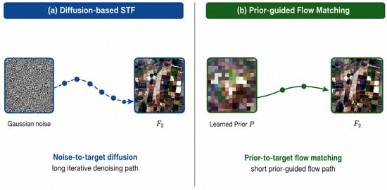
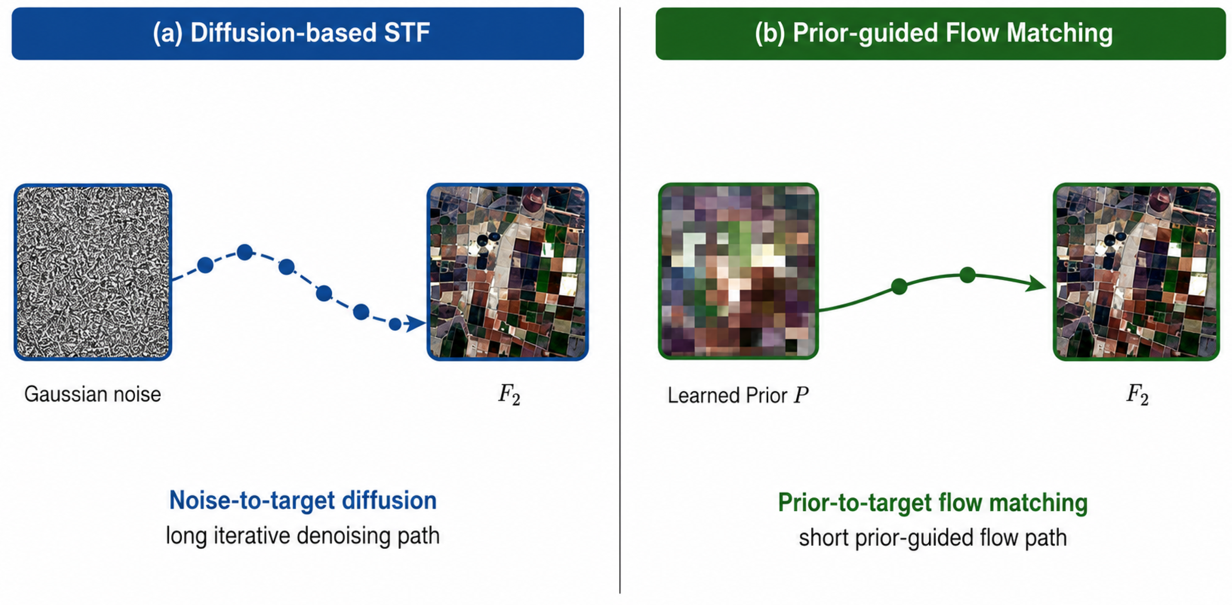
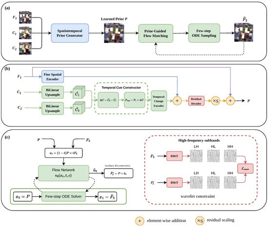
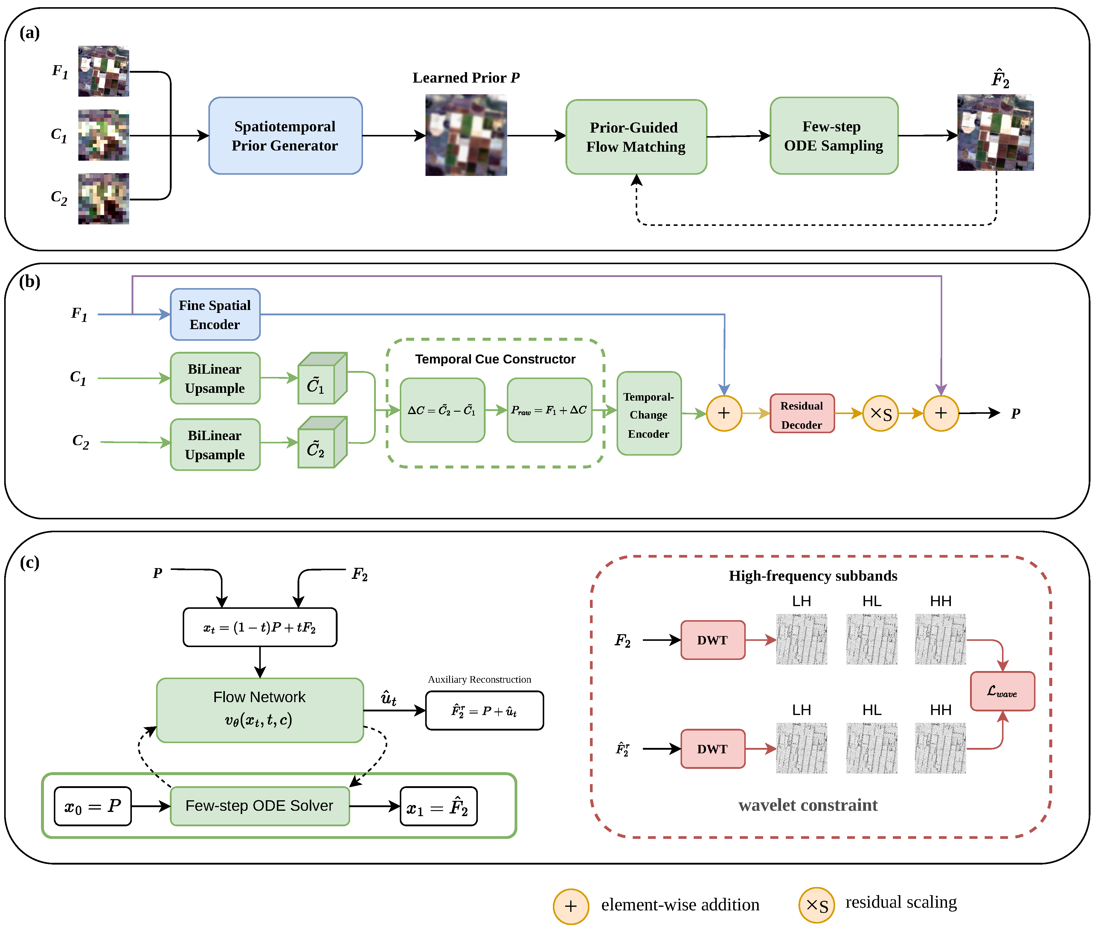
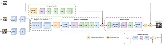
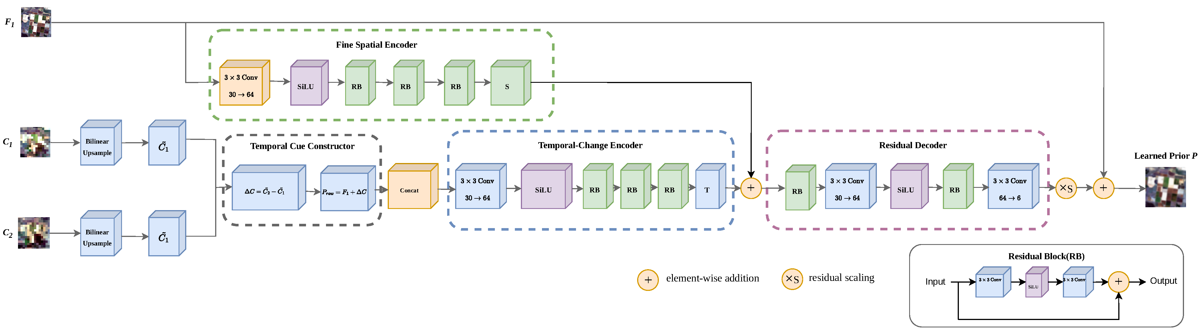
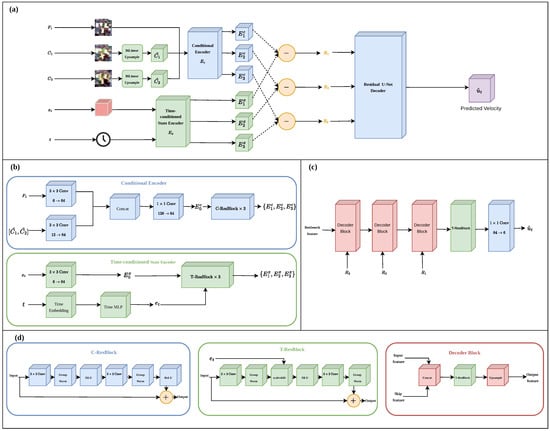
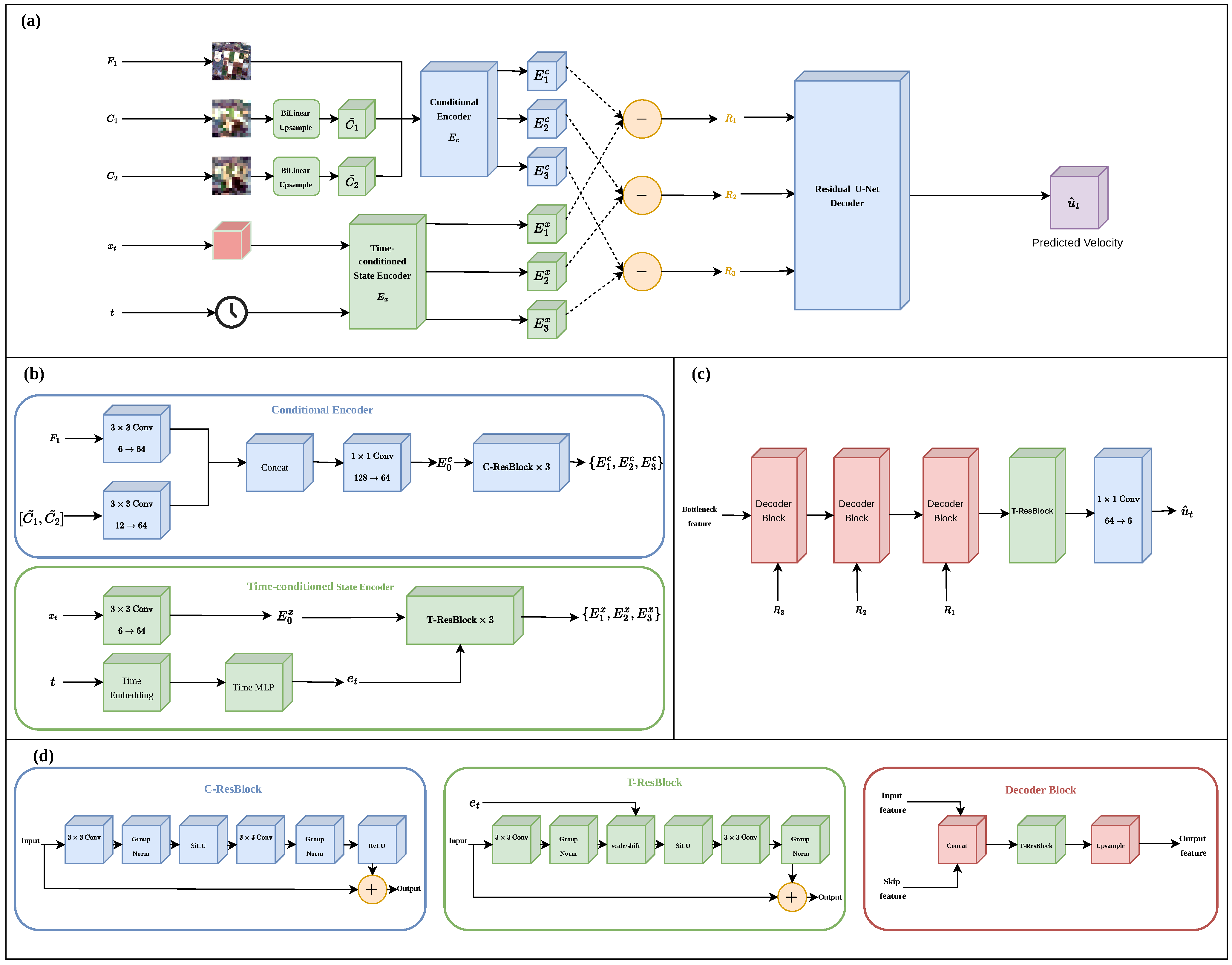
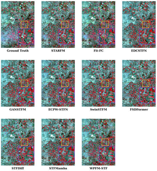
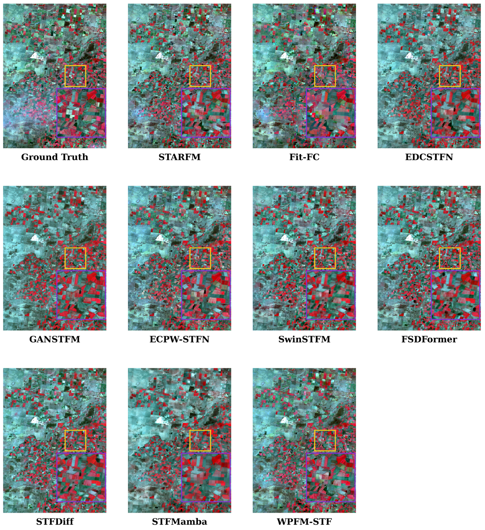
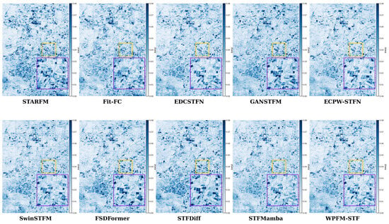
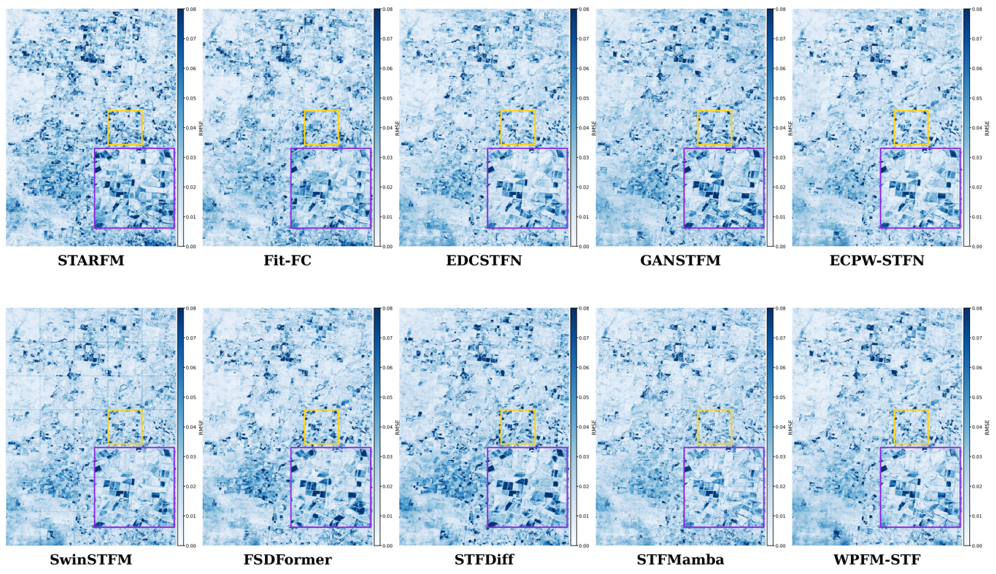
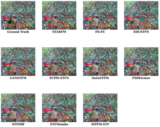
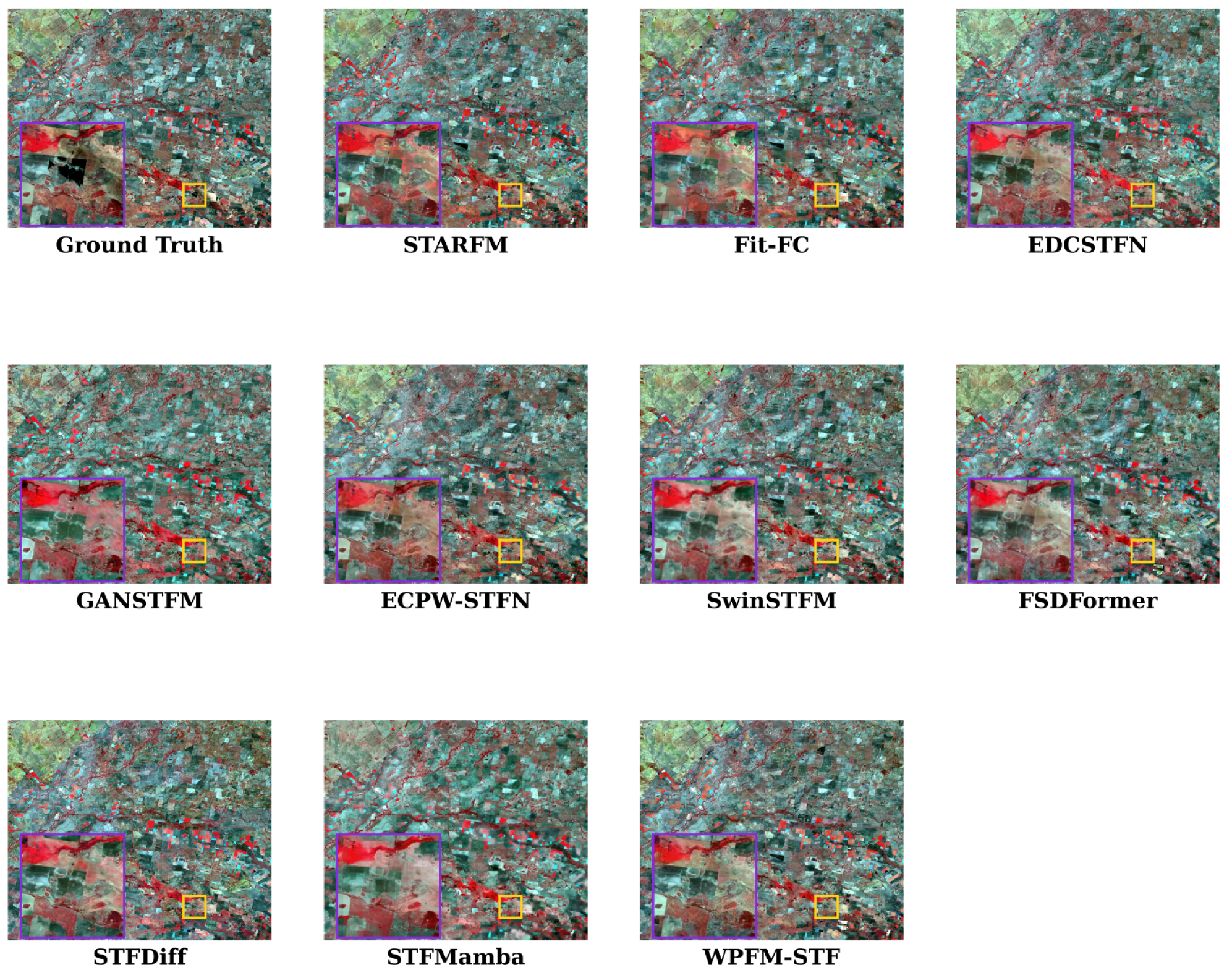
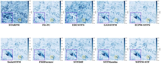
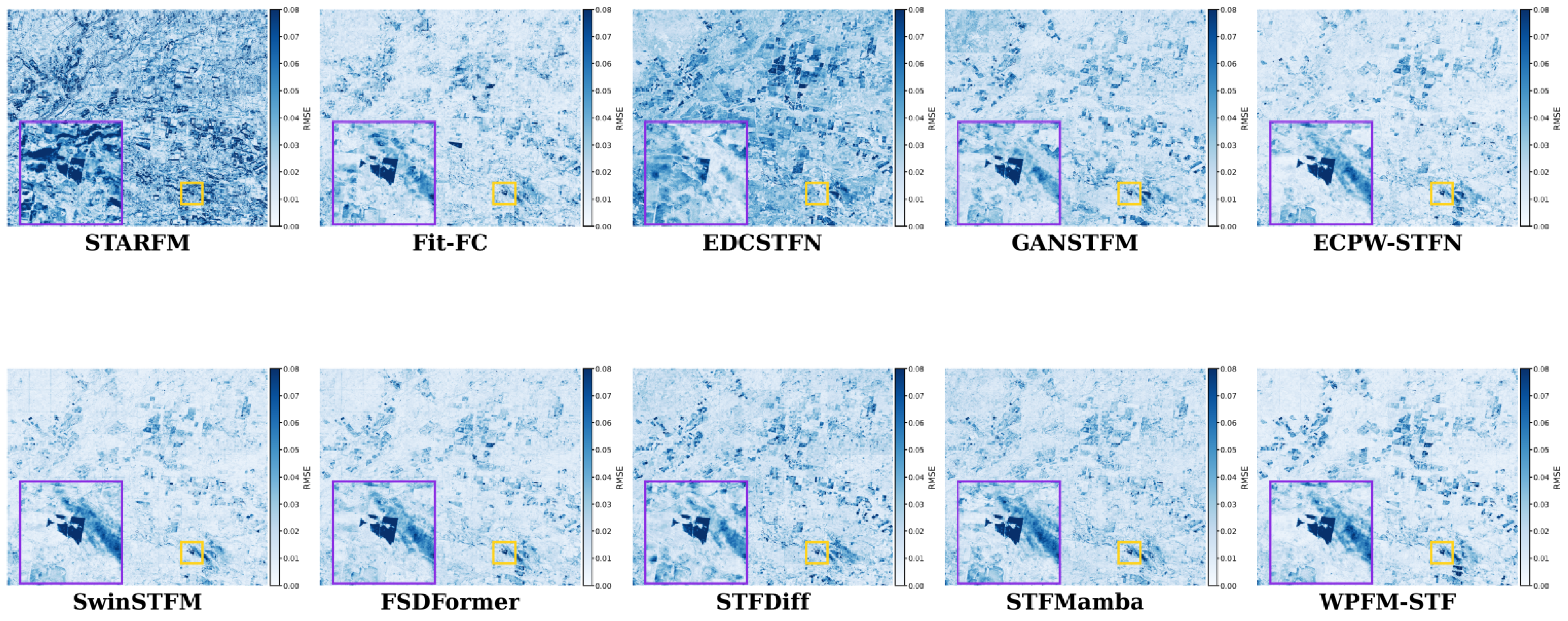
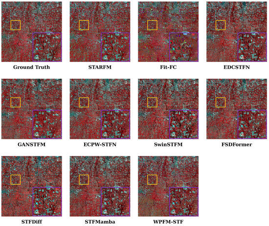
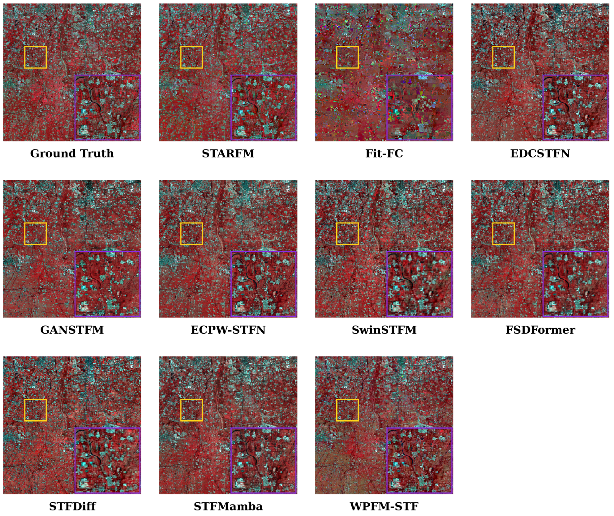
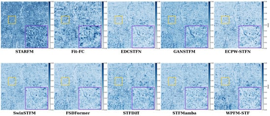
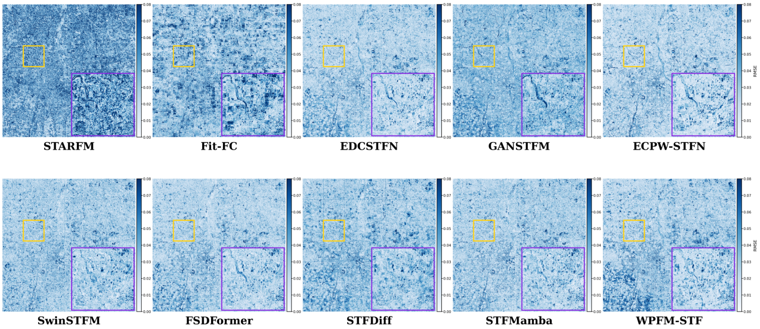
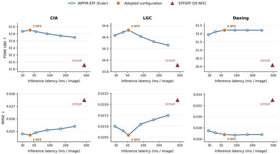
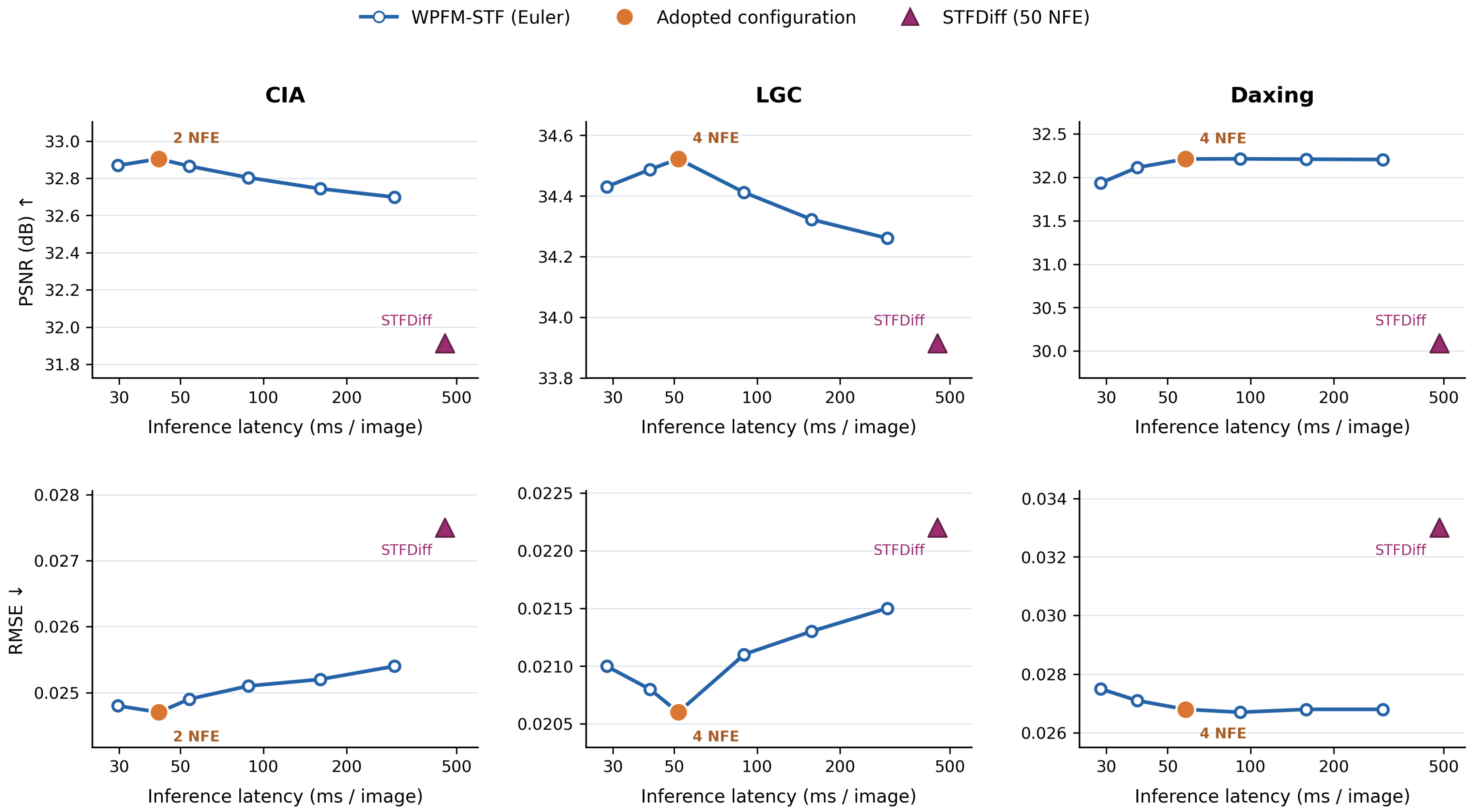
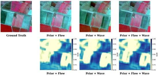
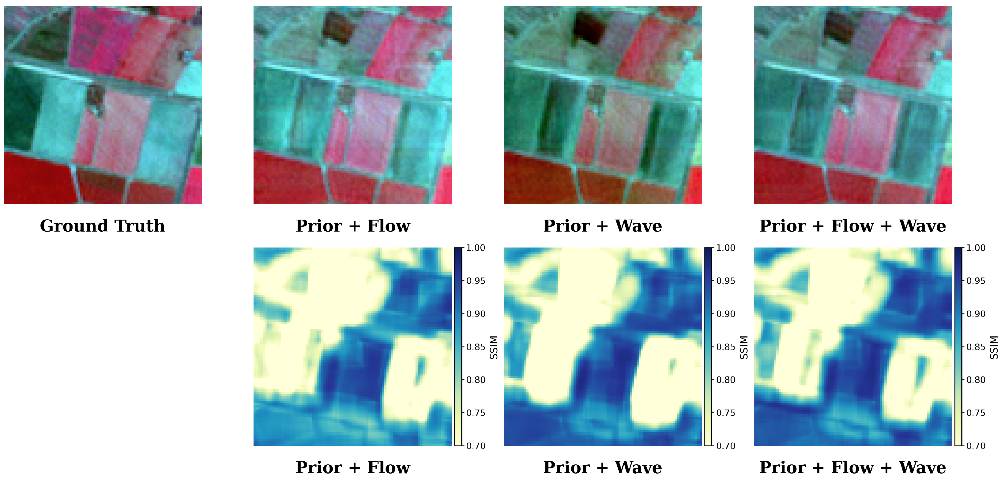
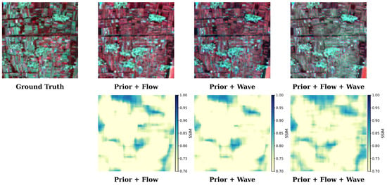
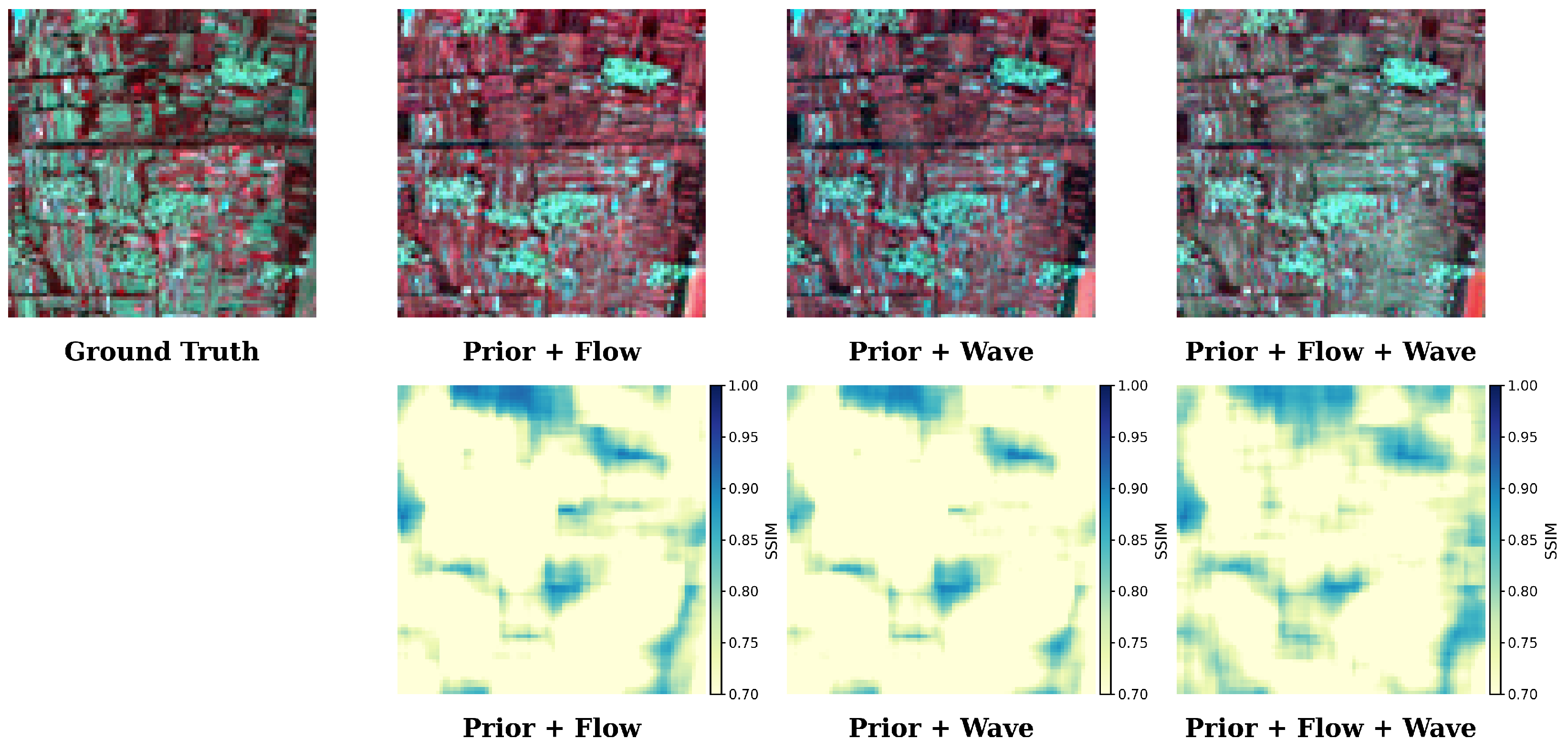
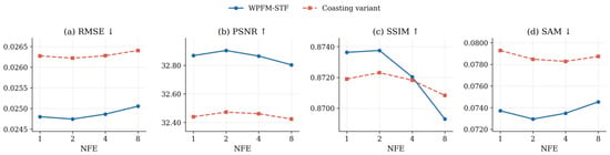
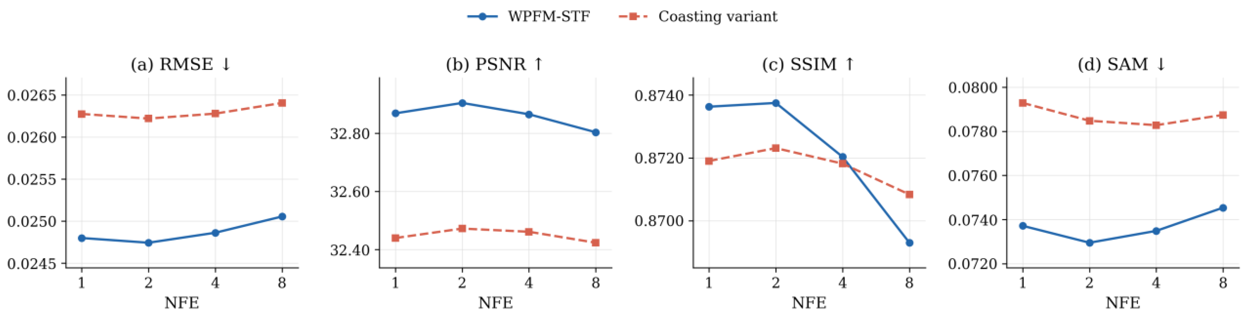
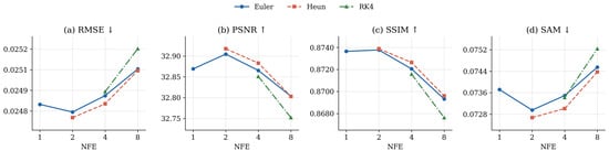
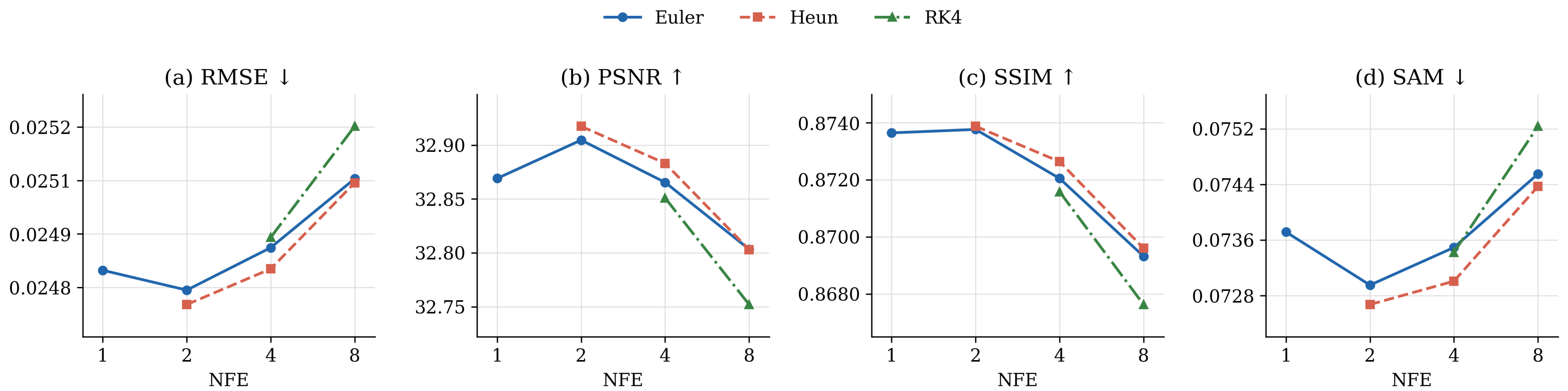
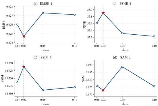
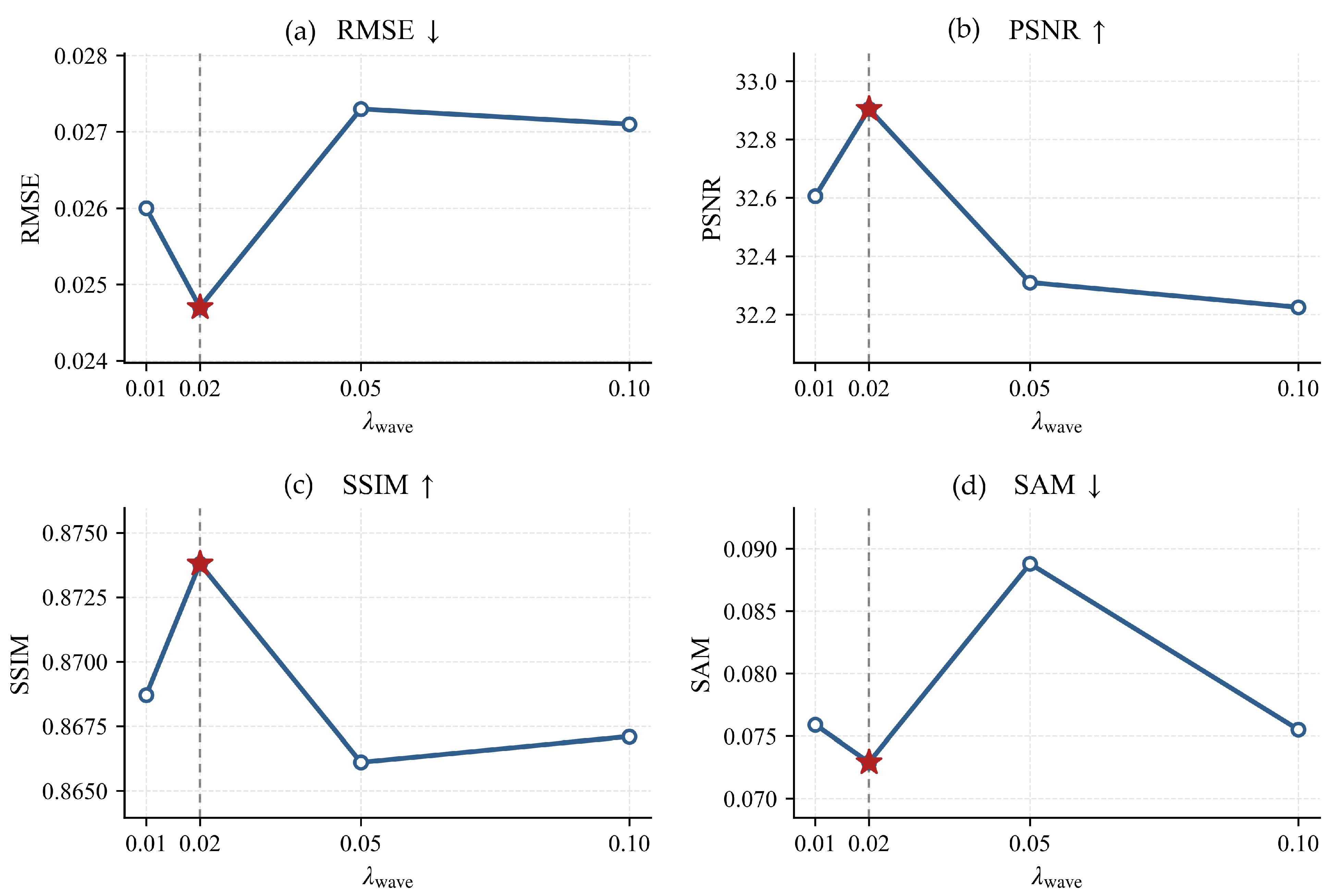
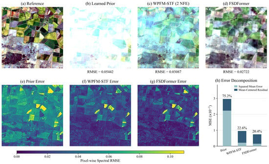
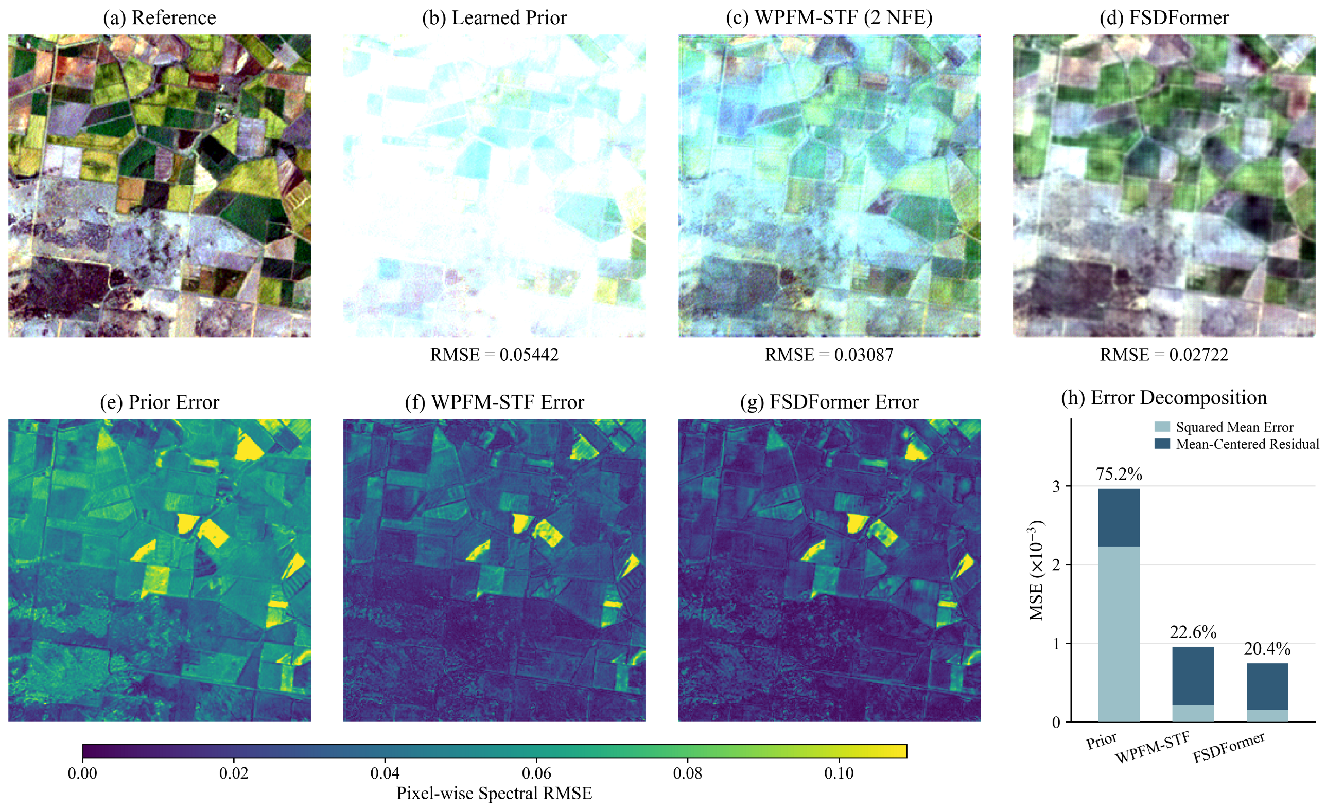

Disclaimer/Publisher’s Note: The statements, opinions and data contained in all publications are solely those of the individual author(s) and contributor(s) and not of MDPI and/or the editor(s). MDPI and/or the editor(s) disclaim responsibility for any injury to people or property resulting from any ideas, methods, instructions or products referred to in the content. |
© 2026 by the authors. Licensee MDPI, Basel, Switzerland. This article is an open access article distributed under the terms and conditions of the Creative Commons Attribution (CC BY) license.