


Highlights
What are the main findings?
- A terrain-constrained workflow combines ascending and descending SBAS-InSAR, deformation-field post-processing, slope units derived using a modified DBSCAN-based method, and bootstrap confidence intervals to screen candidate active-slope units relative to the regional deformation background.
- Across two western China study areas covering approximately 2100 km2, the workflow produced final inventories containing 92 and 25 candidate active-slope units, with inventory-based reference comparison and targeted optical inspection reported as separate evidence streams.
What are the implications of the main findings?
- The method avoids a fixed site-specific deformation-rate cutoff in mm/yr but retains statistical confidence levels and spatial screening criteria, thereby reducing threshold dependence.
- Combining ascending and descending Sentinel-1 geometries increased complementary feasible coverage to 92.17% and 91.96%, respectively, supporting regional inventory updating, hazard reconnaissance, and prioritization of field verification and follow-up monitoring.
Abstract
Landslides are among the most serious geohazards worldwide, and accurately identifying their locations is a prerequisite for effective risk prevention and mitigation. However, regional-scale screening of candidate active-slope units from InSAR observations is still hindered by subjective manual interpretation, inconsistent deformation-rate thresholds, and insufficient topographic constraints. To address these limitations, this study proposes a largely automated terrain-constrained framework for candidate active-slope screening by integrating InSAR observations, slope units, and screening based on slope-unit bootstrap intervals and a regional two-standard-deviation background envelope. First, surface deformation rates are derived from InSAR measurements and post-processed to reduce the influence of identifiable artifacts before slope-unit analysis. Then, a clustering-based method is introduced to delineate topographically constrained slope units in alpine canyon regions, whose visual terrain correspondence is examined qualitatively using terrain information and optical imagery. Next, rather than applying a fixed site-specific deformation-rate cutoff in mm/yr, data-dependent bootstrap confidence-interval comparisons are used to determine whether the deformation interval of each slope unit extends beyond the regional deformation-background interval, thereby enabling rule-based screening of candidate active-slope units. This confidence-interval screening rule provides a quantitative criterion for regional screening but requires further calibration across additional geomorphic and deformation settings. Finally, the proposed method is applied to two landslide-prone regions in western China, located in sections of the Upper Yellow River and Upper Jinsha River, where final inventories containing 92 and 25 candidate active-slope units are produced, respectively. These polygons are geomorphologically constrained candidate active-slope units produced for regional screening and should not be interpreted as the exact boundaries of individual landslides. Inventory-based spatial comparison and targeted optical inspection were reported as complementary evidence streams rather than as independent validation of contemporaneous slope activity. These results document implementation in two related alpine river-valley settings in western China and indicate the framework’s potential as a quantitatively defined, topographically constrained approach for largely automated regional screening of candidate active-slope units in comparable settings. These two applications do not establish broad applicability across substantially different environments.
1. Introduction
Landslides are among the most common and severe geological hazards, causing significant casualties and enormous economic losses worldwide [1,2]. In China, for instance, thousands of landslides are reported annually, resulting in hundreds of fatalities and direct economic losses amounting to tens of billions of CNY [3]. To cope with this serious threat, authorities commonly implement proactive disaster-reduction measures, such as population relocation and early warning systems, to mitigate the impacts of landslides [4]. However, the effective implementation of these strategies faces a critical prerequisite: accurately identifying the locations of potential landslides among numerous slopes.
To address this need and challenge, traditional approaches have relied on field geological surveys. However, such surveys are no longer economically feasible for large areas and often difficult to conduct in complex mountainous terrain [5,6]. Recent advances in Earth observation technologies, particularly high-resolution optical remote sensing and Interferometric Synthetic Aperture Radar (InSAR), have reshaped landslide detection strategies by enabling landslide identification across broad spatial extents [7]. The former is particularly suitable for investigating fresh landslides with significant spectral differences from the surroundings, but faces challenges in detecting potentially active landslides with subtle deformations [4]. By contrast, spaceborne InSAR enables the measurement of subtle surface deformation over wide areas using day-and-night, largely weather-independent SAR acquisitions; however, useful interferometric measurements can still be limited by coherence loss associated with vegetation or snow cover, residual atmospheric effects, and geometric distortions such as layover and shadow [8].
Although previous studies have demonstrated the capability of InSAR to monitor surface deformation at national and regional scales [9,10], the lack of reliable automated interpretation methods still hinders its application in wide-area landslide detection [11]. At present, manual visual interpretation of InSAR results to identify abnormal deformation remains the primary choice in engineering practice [11]. Despite its accuracy and reliability, the method’s inherent inefficiency often precludes its application at large regional scales [12]. To improve efficiency, researchers have attempted to semi-automatically extract potential active landslides from InSAR results by applying deformation rate thresholds. For instance, Dong et al. [13] adopted a threshold of ±8 mm/yr, Liu et al. [10] and Xiong et al. [14] used ±10 mm/yr, whereas Cigna et al. [15] applied ±13 mm/yr. Evidently, a consistent threshold is lacking across different studies, and this process is prone to subjectivity, which may result in high omission and false-alarm rates [11]. On the other hand, with the advancement of deep learning, techniques such as convolutional neural networks (CNN) have made significant progress in automated detection of active landslides [16,17,18]. However, although many recent deep-learning models explicitly incorporate DEM-derived, geological, or multiscale terrain information, some image-centered implementations based on object detection or semantic segmentation may still emphasize image-pattern recognition without explicitly incorporating topographic context [19]. Topographic attributes—such as slope angle, aspect, and elevation—strongly influence slope stability and should therefore be treated as key drivers in detection workflows [20]. In addition, practitioners often encounter practical barriers, including limited access to high-quality training data [21], high computational requirements [22], and poor cross-site generalization [23]. Hence, a clearly defined and operationally applicable approach for regional screening of candidate active-slope units is needed to strengthen the practical implementation of landslide risk management.
Moreover, landslide deformation is governed by complex geomorphological and geological processes, which makes the interpretation of landslide geometry from gridded InSAR data highly diverse [24,25]. To enhance the geological plausibility of landslide boundaries derived from InSAR observations, it is essential to introduce boundary descriptors that explicitly characterize the geometric features of landslides. Slope units represent hydrologically and geomorphologically defined terrain domains, thereby providing effective topographic constraints for active landslide detection [26]. Consequently, this necessitates superior accuracy and quality of slope unit delineation. The goal of slope unit delineation is to obtain partitions with precise boundaries, high internal homogeneity, and clear interunit heterogeneity [27]. Conventional delineation methods based on surface hydrological processes cannot fully capture slope variations beyond flow direction and often require repeated manual correction. Therefore, Huang et al. [28] proposed a multi-scale segmentation method for the efficient and automatic extraction of slope units, and showed that it outperformed the conventional hydrological method in hilly and mountainous areas. Zhang et al. [29] further developed a slope units extraction method based on terrain topology searching and vector similarity constraints, which improves boundary accuracy, internal homogeneity, and interunit heterogeneity. Zeng et al. [30] introduced an object-based image analysis approach, namely refined multi-scale segmentation, to extract regional slope units with limited manual modification. Although these algorithms improve extraction efficiency, their outputs often depend on expert choices of segmentation scale, terrain-topology parameters, vector-similarity thresholds and post-processing corrections; parameter settings calibrated for one geomorphic setting may not transfer well to contrasting landscapes. These limitations motivate the proposed workflow, which likewise involves parameter choices and post-processing but uses adaptive Eps selection and explicit processing criteria to reduce, rather than eliminate, reliance on manual parameter calibration.
To address the practical challenges of regional screening, we propose a largely automated method for identifying candidate active-slope units under topographic constraints. Surface deformation is first retrieved from InSAR observations and then post-processed to remove isolated points and invalid point clusters before slope-unit analysis. We then delineate slope units using a modified DBSCAN-based method with adaptive Eps selection and explicit post-processing criteria, providing terrain-based mapping units for subsequent screening. Building on this, we use bootstrap confidence-interval comparisons to determine whether the deformation interval of each slope unit extends beyond the regional two-standard-deviation background envelope, enabling rule-based screening of candidate active-slope units. The proposed method is finally applied to two representative landslide-prone regions in the upper reaches of the Yellow River and the Jinsha River, where its outputs are assessed through inventory-based reference comparison and targeted optical inspection.
2. Study Area and Datasets
2.1. Study Area
The steep topography, complex lithology, and active tectonics in western China provide favorable conditions for landslide formation [31]. Intense river incision, coupled with ongoing plateau uplift, further destabilizes river valleys, thereby enhancing landslide susceptibility [32]. The upper reaches of the Jinsha River and Yellow River are typical landslide-prone regions with diverse slope geometries and formation mechanisms [33,34], making them representative study areas for applying and validating the proposed method. For clarity, the study area located in the Upper Yellow River is hereafter referred to as Study Area I, and that in the Upper Jinsha River as Study Area II (Figure 1a).
Figure 1.
Geographic location of the study areas: (a) location of the study region and coverage of the SAR dataset; (b) coverage of Study Area I; (c) coverage of Study Area II.
Study Area I is located along a reach of the Yellow River at the boundary between Maqin and Tongde Counties, Qinghai Province, covering an area of approximately 1200 km2 (Figure 1b). The region is characterized by typical plateau-mountain landforms with a mean elevation of ~3800 m. The mean annual precipitation is about 500 mm, most of which is concentrated between May and September [35]. Intense downcutting by the Yellow River has produced steep terrain, with valley flanks generally exceeding 30° and in some places steeper than 50° [36]. The strata consist mainly of Quaternary loess and Neogene red beds (i.e., mudstone and sandstone) [36], while the bedrock has been highly fractured and weakened under the influence of the Lajiasi fault and several subsidiary faults [37]. These factors collectively create a classic landslide-prone environment, providing favorable conditions for the initiation of large-scale landslides.
Study Area II is located on the eastern margin of the Tibetan Plateau, and encompasses the Jinsha River reach between Gongjue and Baiyu counties (Figure 1c). The investigated reach of the Jinsha River is about 48 km long, covering approximately 900 km2. The region has a plateau monsoon climate with annual precipitation of 500~1000 mm, over 80% of which falls between May and September [38]. The landform is a typical alpine gorge with steep terrain, and elevations range from 2500 to 6000 m. Controlled by the Jinsha River tectonic suture zone, the area has a highly complex tectonic framework with large-scale faults and folds [39]. The strata mainly consist of sedimentary rocks (e.g., sandstone, limestone) and metamorphic rocks (e.g., schist, mica schist), with the bedrock being widely fractured [39]. Combined effects of strong tectonic activity, persistent river incision, weathering, and unloading have destabilized valley slopes, leading to frequent landslides.
2.2. Datasets
In this study, open-access Sentinel-1 synthetic aperture radar (SAR) data provided by the European Space Agency (ESA) were employed to derive surface deformation. Sentinel-1A operates at C-band with a wavelength of 5.60 cm, native azimuth and range pixel spacings of 13.99 m × 2.33 m, and a revisit interval of 12 days. Specifically, Single Look Complex (SLC) images acquired in Interferometric Wide (IW) mode with VV polarization were processed using the InSAR technique. The values of 13.99 m and 2.33 m refer to the native azimuth and slant-range sampling spacings of the Sentinel-1 SLC data, respectively, rather than to the grid spacing of the final geocoded deformation products. After multilooking in the range and azimuth directions and subsequent geocoding in SARscape using the Optimal Resolution setting, all four final RADRM products were exported to a 12.5 m × 12.5 m square grid in the WGS 1984 Web Mercator Auxiliary Sphere coordinate system (EPSG:3857). The 12.5 m value denotes the projected output-grid spacing and should not be interpreted as the effective spatial resolution, because multilooking and geocoding alter the spatial response, and resampling does not restore spatial information lost during processing. The spatial coverage of SAR datasets for Study Areas I and II is shown in Figure 1a, with detailed parameter information summarized in Table 1. In addition, a 30 m resolution digital elevation model (DEM) from the ALOS World 3D dataset was used as the primary input for slope unit delineation and topographic phase simulation. GACOS products were incorporated to correct atmospheric phase delays in the interferograms, which are especially significant in alpine canyon regions. Finally, multitemporal Google Earth and Jilin-1 optical imagery spanning the full Sentinel-1 observation periods (January 2020–December 2023 for Study Area I and January 2020–May 2022 for Study Area II; Table 1) was used as supplementary evidence for interpreting the identified candidate active-slope units, rather than as independent evidence of contemporaneous activity.
Table 1.
Data information for the study areas.
Because of the side-looking imaging geometry of SAR, steep alpine canyon terrain is prone to severe geometric distortions. We therefore analyzed the geometric distortions of the Sentinel-1 dataset using the SAR imaging geometry and the DEM [40]. All geometric-distortion results were calculated on a common DEM-based grid within the same study-area mask. For each viewing geometry, the percentage of each terrain-geometry category was obtained by dividing the number of pixels assigned to that category by the total number of valid pixels within the study area and multiplying the result by 100. The combined feasible coverage was determined by overlaying the ascending- and descending-orbit feasible-observation masks pixel by pixel and calculating the proportion of study-area pixels that were feasible in at least one viewing geometry. Pixels feasible in both viewing geometries were therefore counted only once rather than being added twice. All totals were calculated from unrounded pixel counts, and minor differences of 0.01% in the displayed sums result from rounding. Figure 2 summarizes the results for Study Area I. For the ascending images, layover, shadow, foreshortening, and feasible observation pixels account for 24.92%, 17.96%, 0.35%, and 56.76% of the area, respectively; in the descending images the corresponding percentages are 3.61%, 6.32%, 0.31%, and 89.77%. By combining both viewing geometries, the complementary feasible observation coverage increased to 92.17% because areas affected by layover or shadow in one geometry may remain observable in the other. Figure 3 shows analogous statistics for Study Area II. In Study Area II, layover, shadow, foreshortening, and visible areas account for 18.59%, 2.89%, 3.85%, and 74.67% of the area in the ascending dataset, and 10.92%, 4.81%, 2.51%, and 81.76% in the descending dataset. Jointly, the two geometries yield a feasible coverage of 91.96%. Overall, the joint use of ascending and descending SAR images increases complementary feasible coverage but does not correct or remove the geometric distortions present in the individual acquisitions.
Figure 2.
Geometric distortion and visibility analysis for Study Area I. Panels (a,d) show areas of layover, shadow, foreshortening, and feasible observation for ascending orbit data; (b,e) for descending orbit data; and (c,f) for the combination of ascending and descending Sentinel-1 images.
Figure 3.
Geometric distortion and visibility analysis for Study Area II. Panels (a,d) show areas of layover, shadow, foreshortening, and feasible observation for ascending orbit data; (b,e) for descending orbit data; and (c,f) for the combination of ascending and descending Sentinel-1 images.
3. Methods
3.1. Using SBAS-InSAR to Measure Land Surface Deformation
Given the requirements of landslide detection, we processed the Sentinel-1 SAR datasets using the Small Baseline Subset InSAR (SBAS-InSAR) technique originally proposed by Berardino et al. [41]. This method generates interferograms from SAR image pairs with short temporal and spatial baselines, thereby minimizing spatio-temporal decorrelation and atmospheric effects and enabling millimeter-scale sensitivity to surface deformation under suitable observation and processing conditions [42]. A detailed description of the fundamental principles and processing workflow of SBAS-InSAR can be found in Tizzani et al. [43] and Zhao et al. [44].
The SBAS-InSAR calculations were performed using the SBAS module of SARscape 5.6.2 within the ENVI 5.6 environment. Prior to interferometric processing, the SAR images and ancillary data were preprocessed, including precise orbit correction and image co-registration. To suppress speckle noise, multilooking factors of 5 and 1 were applied in the range and azimuth directions, respectively. Accordingly, before geocoding, the nominal sampling intervals were approximately 11.65 m in slant range and 13.99 m in azimuth. These sampling intervals describe raster sampling rather than effective ground resolution. The maximum temporal baselines for Study Areas I and II were set to 150 and 48 days, respectively, because the latter exhibits poorer coherence due to dense vegetation. The perpendicular baseline was limited to 150 m for both areas. After generating interferograms under these criteria, an adaptive Goldstein filter based on the local fringe spectrum was applied to suppress phase noise [45]. Phase unwrapping was then performed on pixels with high coherence using the minimum cost flow (MCF) algorithm [46,47]. Because atmospheric delays are more pronounced in humid climates and steep terrain, GACOS products were used for atmospheric correction of the unwrapped phase [48], followed by a polynomial model to remove residual errors. Finally, we solved the observation equations derived from the high-quality unwrapped interferograms using singular value decomposition (SVD), yielding the line-of-sight (LOS) displacement time series and the deformation rate map. Because the deformation-rate map provides a more robust representation of long-term deformation trends [49], it was geocoded in SARscape using the Optimal Resolution setting and exported to a 12.5 m × 12.5 m square grid in the WGS 1984 Web Mercator Auxiliary Sphere coordinate system (EPSG:3857). All four final RADRM products used this output-grid specification. The 12.5 m value represents the projected output-grid spacing rather than the effective spatial resolution of the deformation measurements. The SBAS-InSAR processing followed the established workflows described in Refs. [41,42,43,44]. Because the resulting deformation-rate map was used as an upstream input for regional screening of candidate active-slope units rather than for site-specific geodetic interpretation, Section 3.1 reports the study-specific settings directly relevant to the detection framework without reproducing the complete software-level processing record.
3.2. Post-Processing of InSAR Deformation Rate Results
The deformation rate map derived in Section 3.1 still contains artifacts resulting from SAR geometric distortions, phase unwrapping errors, and residual atmospheric delays [50]. Therefore, we performed an additional post-processing step on the raw deformation rate (RDR) map to attenuate these artifacts before candidate active-slope screening.
3.2.1. Removal of False Deformation Signals
We first used the C-index as a directional-consistency filter to screen pixels whose deformation-rate sign was inconsistent with the theoretically expected LOS direction. The C-index is derived from the DEM and SAR imaging geometry, as shown in the following equation [14]:
where θ and γ denote the incidence and heading angles, respectively, and φ and β represent the slope gradient and aspect, respectively. The C-index ranges from −1 to 1, with its magnitude and sign reflecting the theoretical sensitivity and direction of LOS deformation, respectively. Typically, LOS deformation is defined as positive when a landslide moves toward the radar and negative when it moves away. Based on this principle, the following directional-consistency screening rule was adopted: if the sign of a pixel’s InSAR deformation rate is consistent with the sign of its C-index, or if its C-index is equal to zero, the pixel is provisionally retained at this stage; otherwise, it is excluded by the directional-consistency rule [14].
The C-index was used only to assess the directional consistency between the observed LOS deformation and the assumed slope movement direction. Its magnitude was not used as an independent filtering threshold; therefore, zero or near-zero C-index values were retained unless the inferred deformation direction was inconsistent with the expected slope movement direction.
3.2.2. Removal of Isolated Points
After false deformation signals were removed, some isolated deformation points may still remain in the results, typically defined as those without any neighboring pixels in the deformation results [51]. This is mainly attributable to strong decorrelation in complex terrain or densely vegetated areas [52], which leads to a sparse distribution of valid measurements, as well as to spatially uncorrelated isolated noise. Therefore, building upon the deformation rate results filtered in Section 3.2.1, a local neighborhood analysis was further applied to each pixel in the spatial domain. All distances were calculated as Euclidean distances between pixel-center coordinates in the projected coordinate system (EPSG:3857), rather than from raster row and column indices. Let denote the projected spacing of the final geocoded grid. For each target pixel, neighboring valid deformation pixels were searched using the strict distance criterion . On the square grid, this criterion includes the four edge-sharing pixels at a distance of and the four diagonally adjacent pixels at a distance of , while excluding pixels at distances of or greater. A target pixel was classified as isolated and discarded only when no other valid deformation pixel occurred within this eight-neighbor spatial neighborhood [51].
3.2.3. Removal of Invalid Point Clusters
The preceding steps filtered false and isolated deformation signals at the pixel level; however, the results may still be affected by noise. Such noise often shows spatial correlation; for instance, atmospheric residuals, unwrapping errors, or occasional aggregation of random noise can form localized invalid point clusters rather than purely random isolated pixels [53]. These spatially correlated artifacts reduce the interpretability of the InSAR deformation rate map, thereby hindering landslide detection [54]. To address this issue, we performed spatial clustering based on the results of Section 3.2.2 to remove invalid point clusters.
Regional InSAR deformation-rate distributions are generally dominated by measurements from the stable background, whereas genuine deformation and residual processing artifacts may produce departures in the distribution tails. Accordingly, the mean (μ) and standard deviation (σ) were calculated separately for each deformation-rate dataset, and the μ ± 2σ interval was used as a descriptive, data-dependent screening rule [50]. Pixels outside this interval were provisionally identified as candidate active deformation area (ADA) pixels, whereas those within the interval were provisionally classified as non-active deformation area (NDA) pixels. This screening operation does not assume that the complete regional distribution is strictly Gaussian and is not used as a formal probabilistic classification. Heavy-tailed departures are retained as candidate anomalies and are subsequently evaluated using the spatial-clustering criteria described below. Thus, the workflow avoids a fixed site-specific deformation-rate threshold in mm/yr while retaining explicit statistical and spatial screening criteria.
Subsequently, ADA pixels were extracted from the deformation-rate map filtered in Section 3.2.2 and spatially clustered in the projected coordinate system [55]. The Euclidean distance between pixel centers was used, with a clustering radius of [51], where is the projected spacing of the final geocoded grid. Because the distance between diagonally adjacent pixel centers is , the selected radius connects edge-sharing pixels but not diagonally adjacent pixels, corresponding to four-neighbor connectivity on the output grid. Previous Sentinel-1-based ADA mapping studies commonly impose a minimum cluster size to suppress isolated or noise-driven detections. According to the Guideline of InSAR Monitoring for Geo-hazard (T/CAGHP 013-2018) issued in China [56], at least 30 pixels are required to identify and monitor an individual landslide. Therefore, clusters containing fewer than 30 pixels were treated as invalid and excluded from further analysis. Each output-grid cell represents a nominal mapped area of ; consequently, 30 pixels correspond to a nominal mapped area of , or approximately . Because these calculations were performed in EPSG:3857, the thresholds are reported as projected map distances and nominal mapped areas rather than exact geodesic ground distances and areas. Importantly, the μ ± 2σ partition is used only to identify candidate ADA pixels for subsequent spatial screening and is not regarded as a definitive pixel-level discrimination between genuine deformation and noise. Pixels classified as NDA are not discarded. After ADA clusters containing fewer than 30 pixels are removed, the retained ADA pixels are recombined with all NDA pixels to construct the refined annual deformation rate map (RADRM). Slope-unit candidate status is subsequently assessed using the bootstrap confidence-interval comparison described in Section 3.4. Together with the GACOS and polynomial atmospheric corrections applied in Section 3.1 and the C-index and isolated-pixel filters applied in Section 3.2.1 and Section 3.2.2, this sequential procedure reduces potential ADA/NDA misclassification caused by residual atmospheric and processing noise. Nevertheless, broad spatially correlated residuals that satisfy all the preceding physical and spatial criteria cannot be completely excluded.
3.3. Slope-Unit Extraction Using a Modified DBSCAN-Based Method
The essence of slope-unit delineation is to partition the study area into a series of subregions that are internally homogeneous and externally heterogeneous with respect to topographic attributes such as slope and aspect [27]. Building on this concept, slope-unit delineation can be formulated as a clustering problem in which each resulting slope unit corresponds to a spatially connected cluster. In this study, a modified DBSCAN-based method was implemented to delineate preliminary slope units in a standardized feature–spatial space. The method retains the Eps-neighborhood search and connectivity-expansion mechanism of density-based spatial clustering of applications with noise (DBSCAN) [57] but does not use the conventional distinction among core, border, and noise points.
The actual implementation is illustrated in Figure 4. Each valid DEM pixel was represented as a node in the standardized feature–spatial space. For any two pixels P and Q, an undirected edge was established when their standardized Euclidean distance did not exceed Eps. Preliminary slope units were then obtained by extracting the connected components of the resulting Eps-neighborhood graph. Because MinPts was set to 0, every valid pixel was allowed to participate in the connectivity expansion, and no separate border-point or noise-point classes were defined. Under this configuration, the method is mathematically equivalent to connected-component extraction from an Eps-neighborhood graph, although its neighborhood search and iterative cluster-expansion procedure were implemented within a DBSCAN-based computational framework.
Figure 4.
Schematic illustration of the modified DBSCAN-based procedure used in this study. Valid pixels are represented as nodes, and two nodes are connected when their standardized Euclidean distance does not exceed Eps. Each connected component of the resulting Eps-neighborhood graph is extracted as a preliminary slope unit.
The raw DEM was Gaussian-smoothed, and slope aspect was derived to capture subtle terrain differences between adjacent units [58]. Before clustering, the two Cartesian coordinates x and y and the sine-transformed aspect variable sin(απ/180) were independently Z-score standardized within each study area, and no additional manual feature weights were applied. Euclidean distances were then calculated in the resulting three-dimensional standardized feature–spatial space [59]. Accordingly, each standardized dimension entered the distance calculation with a coefficient of 1, with spatial location represented by two dimensions and slope aspect represented by one dimension. The parameter k = 1 was used only to construct the nearest-neighbor distance curve for Eps determination [60]. The study-area-specific Eps value was subsequently determined using the improved tangential-angle method of Xu et al. [61], with Eps defined as the k-distance corresponding to the last point at which the improved tangential angle reached 45° (Figure 5). The modified DBSCAN-based connectivity procedure was then applied to the standardized variables to generate the preliminary slope units. To remove small, fragmented, or over-subdivided clusters that lack geomorphological meaning and impair within-unit homogeneity and analytical stability [29,62], the minimum-area constraint and the rule for merging undersized units with adjacent geomorphologically coherent units were adopted from the established procedure in [63]. Boundary smoothing was performed as a basic geometric post-processing operation rather than as an additional criterion for clustering or slope-activity classification. The specific implementation settings and post-processing rules were as follows. In both study areas, the 30 m DEM was smoothed using a Gaussian filter with a standard deviation of sigma = 1.6 DEM pixels and a 7×7-pixel kernel, corresponding to 48 m and 210×210 m, respectively. These Gaussian-filter parameters were selected through an empirical sensitivity assessment. After the preliminary slope units were extracted, a minimum-area threshold of 20,000 m2 was applied following the referenced slope-unit delineation procedure [63]. Units below this threshold were processed iteratively in ascending order of area. Only units sharing a common boundary were considered neighbors. When an undersized unit had multiple neighboring units, it was merged with the neighbor sharing the longest boundary; if two or more neighbors had the same shared-boundary length, the neighbor with the largest area was selected. The polygon geometry, area, shared-boundary lengths, and associated merging attributes were recalculated after each merge, and the procedure was repeated until no unit smaller than 20,000 m2 remained. The merged polygons were subsequently smoothed using the Smooth Polygon tool in ArcGIS 10.7 with the PAEK algorithm and a smoothing tolerance of 1000 m. In the PAEK algorithm, this tolerance defines the length of the moving path used to calculate the smoothed vertices and should not be interpreted as the maximum displacement of the polygon boundary. The 1000 m value was selected through empirical parameter trials and visual comparison, with the practical aim of reducing raster-derived angularity while seeking to retain visually recognizable ridge- and valley-controlled boundaries. It was not selected through quantitative optimization based on within-unit homogeneity or between-unit heterogeneity and should therefore not be interpreted as a universally optimal value. No barrier layer was specified. Topological-error checking was enabled using the FLAG_ERRORS option, and all output records had SmoPgnFlag = 0. This result indicates only that no topological errors were flagged by the tool; it does not independently demonstrate that the geomorphological boundaries were preserved. Thus, the automated post-processing order was minimum-area-based iterative merging followed by PAEK polygon smoothing. The final units were then visually inspected as a rapid quality-control step, and only visibly anomalous boundaries were locally corrected. Because these corrections were made during routine inspection rather than as a separately logged processing stage, their number was not systematically recorded.
Figure 5.
Flowchart of the slope unit delineation process.
3.4. Confidence-Interval-Based Screening of Candidate Active-Slope Units
Overlaying the gridded refined annual deformation rate map (RADRM) onto slope units yields slope unit objects with associated deformation information. Relative to the stable background, active slopes typically exhibit pronounced deformation signals, providing an important basis for active landslide detection [25]. Although this idea is straightforward, its practical implementation still lacks standardized quantitative criteria and continues to rely on expert judgment or manual interpretation. Therefore, we introduce a bootstrap confidence-interval comparison framework to quantitatively determine whether the deformation interval of each slope unit extends beyond the regional deformation-background interval, thereby identifying candidate slope units whose mean deformation behavior extends beyond the regional background envelope. This interval comparison is used as a rule-based screening criterion rather than as a conventional null-hypothesis significance test. The procedure comprises the following steps:
(1) Coregister the slope units and the RADRM onto a common spatial grid, and extract the corresponding RADRM values for each slope unit.
(2) To characterize regional background variability, all valid RADRM pixel values within the complete study area were used to calculate the regional mean and sample standard deviation. For each study area and each RADRM dataset, let denote the total number of valid regional pixels and the deformation rate of the pixel indexed by . The regional mean and sample standard deviation were calculated as follows:
The regional background envelope was then defined as:
where the regional mean and regional sample standard deviation were calculated from all valid regional RADRM pixel values after the same preprocessing and data-quality screening. This range is a two-standard-deviation regional background envelope rather than a bootstrap confidence interval or an empirical percentile interval. Although a mean ± two-standard-deviation range contains approximately 95% of observations under an ideal normal distribution, no exact 95% coverage was assumed because the regional pixel distribution may be non-normal and spatially correlated.
(3) Estimate the confidence interval for the arithmetic mean deformation rate within each slope unit. Because certain slope units contain relatively few valid InSAR deformation pixels, we used the basic bootstrap method to estimate confidence intervals for the slope-unit mean. Bootstrap resampling is a widely used statistical technique that is particularly suited to small-sample estimation [64]. For each slope unit in each orbit-specific RADRM dataset, the number of valid RADRM pixels was first determined. An operational minimum of 30 valid RADRM pixels was required for bootstrap-based candidate screening. Slope units containing 1–29 valid RADRM pixels were marked as insufficiently observed, whereas units containing zero valid pixels were recorded as having no valid observations. Both categories were excluded from the bootstrap analysis, and no inference regarding their activity status was made. For slope units containing at least 30 valid RADRM pixels, bootstrap resampling was performed to estimate the confidence interval of the arithmetic mean deformation rate. Individual valid RADRM pixels were used as resampling units without explicitly accounting for their spatial dependence. The 30-pixel requirement was used only as a pixel-support criterion and does not imply that a slope unit contains at least 30 independent observations. The basic bootstrap procedure is as follows:
For slope unit , let the RADRM sample be denoted by , where is the deformation rate of pixel and is the number of valid RADRM pixels in the slope unit. The bootstrap analysis was implemented using a custom MATLAB (R2023a) program, principally using the datasample, prctile, and mean functions. The number of bootstrap replications was set to B = 1000. For each slope unit containing mi valid RADRM pixels, each replication sampled mi values with replacement from the original unit-level pixel sample. The numerical stability of the interval endpoints was examined by increasing B from 100 to 1000 in increments of 50 and comparing the resulting lower and upper interval limits with those obtained at B = 1000. The median and 95th-percentile absolute endpoint differences decreased progressively as B increased and had become small by B = 900–950. Therefore, B = 1000 was retained as a conservative setting for the final slope-unit interval calculations. During bootstrap replication , the same number of values is sampled with replacement from the original slope-unit sample to obtain . Repeating this procedure times yields the bootstrap distribution. The arithmetic means of the original and resampled samples are defined as follows [64]:
where is the arithmetic mean of the original RADRM sample and is the mean calculated from bootstrap replication . Let denote the empirical th quantile of the bootstrap-mean distribution obtained from replications. The basic bootstrap confidence interval for the slope-unit mean is:
In this study, the significance level was set to ; therefore, the 95% basic bootstrap confidence interval for the arithmetic mean deformation rate of each slope unit is:
(4) The regional background envelope and the slope-unit bootstrap interval have different statistical roles. The regional envelope describes the dispersion of pixel-level deformation rates across the complete study area, whereas the 95% basic bootstrap interval quantifies the sampling uncertainty of the mean deformation rate within an individual slope unit. They were compared as an operational screening rule rather than as two confidence intervals estimating the same quantity. Let denote the 95% basic bootstrap interval for slope unit and the regional background envelope. A slope unit was classified as non-active when its complete bootstrap interval was contained within the regional background envelope (Figure 6b):
Figure 6.
Schematic diagram for screening candidate active-slope units. The upper histograms show the distribution of pixel-level deformation-rate values within each slope unit. Bootstrap resampling of these pixel values was used to estimate the confidence intervals of the mean deformation rate; the histograms themselves do not represent bootstrap means. (a) Schematic diagram for calculating the regional background envelope; (b) Schematic diagram for calculating the confidence interval for units not selected as candidates; (c) Schematic diagram for calculating the confidence interval for candidate active-slope units.
Otherwise, when the slope-unit interval extended partially or completely beyond the regional background envelope, the unit was identified as a candidate active-slope unit (Figure 6c):
Because deformation associated with a large or complex active slope may span multiple adjacent slope units, preliminary candidate active-slope units that may represent the same spatially continuous deformation feature are merged. Specifically, the merging of two adjacent slope units is performed only if the following criteria are simultaneously satisfied: (i) the two units share a common boundary; (ii) at least one pair of ADA pixels is contiguous across the boundary; and (iii) the two units have a mean slope-aspect difference of less than 30°, which was adopted as a study-specific tolerance following the general aspect-similarity principle used in slope-unit merging [63]. The resulting merged unit is treated as a single merged candidate active-slope unit and should not be interpreted as the exact polygon of an individual landslide.
3.5. Implementation Procedure
This section details the implementation of the largely automated workflow for screening candidate active-slope units under topographic constraints, as illustrated in Figure 7. The procedure comprises four stages: (i) RDR data is first obtained using SBAS-InSAR processing; (ii) the RDR is subsequently post-processed to suppress noise, producing RADRM for landslide analysis; (iii) slope units are delineated using the modified DBSCAN-based method to provide topographic boundary constraints for the screening task; (iv) RADRM data are integrated with the slope units, and the operational comparison between slope-unit bootstrap intervals and the regional background envelope serves as the screening rule for candidate active-slope units.
Figure 7.
Workflow of the proposed rule-based screening method for candidate active-slope units.
For the two complementary reference-comparison streams, the units of analysis were defined separately. In the inventory-based spatial-correspondence assessment, each mapped landslide polygon was treated as one independent reference object. If multiple mapped landslides occurred within a single final candidate active-slope unit, each mapped landslide was counted separately. If one mapped landslide intersected multiple final candidate active-slope units, all intersection geometries were combined and the mapped landslide was counted only once. For each mapped landslide, the total historical-landslide coverage fraction was calculated as the area of the union of all intersections with final candidate active-slope units divided by the mapped landslide area. Boundary-only contact with zero intersection area was not considered a spatial correspondence. Two complementary criteria were reported: strict positive-area correspondence, defined by any non-zero intersection area, and substantive spatial correspondence, defined using a minimum historical-landslide coverage threshold of 1%. The sensitivity of the spatial-correspondence counts to higher coverage thresholds was also examined.
In the candidate-level reference-support assessment, each final candidate active-slope unit was treated as one analysis unit and counted only once, regardless of the number of mapped landslides it contained or intersected. A candidate unit was considered supported by the available reference information if it had a positive-area intersection with at least one mapped landslide, showed recognizable landslide-related geomorphic signatures in the inspected optical imagery, or both. Accordingly, a candidate unit intersecting multiple mapped landslides contributed one reference-supported candidate, whereas multiple candidate units intersecting the same mapped landslide were counted separately at the candidate-unit level. Candidates for which neither form of support was identified were recorded as having no support identified in the available reference information. They were not classified as verified absent, false positives, or inactive units. Recognizable geomorphic signatures in the optical imagery were used only as evidence of landslide-related morphology and were not treated as independent confirmation of activity during the corresponding InSAR observation period. Because the available reference information did not establish an independent positive or negative activity status for every final candidate unit, no TP/FP classification or precision estimate was calculated.
4. Results and Analysis
4.1. Results of Study Area I on the Yellow River
4.1.1. Deformation and Its Post-Processing
Based on the Sentinel-1 data described in Section 2.2, we applied the SBAS-InSAR method to derive surface RDR maps from ascending and descending tracks for Study Area I (Figure 8a,c). Histograms of annual deformation rates were constructed for each RDR dataset. Gaussian curves were superimposed only as visual references for the central distribution dominated by the stable-background measurements. Departures in the distribution tails were preserved and treated as candidate deformation anomalies rather than excluded as deviations from normality. Accordingly, these reference curves are not intended to demonstrate that the complete regional distribution, which contains both stable and deforming populations, follows a Gaussian model (Figure 8b,d). The mean-and-standard-deviation classes shown in the map legends of Study Area I are defined using the corresponding mean (μ) and standard deviation (σ) values of the ascending- and descending-track deformation-rate distributions reported in Figure 8, respectively.
Figure 8.
Initial annual deformation rate maps and corresponding distributions for Study Area I: (a,c) ascending and descending orbit RDR maps, respectively; (b,d) corresponding PDFs. The Min and Max values in (b,d) denote the minimum and maximum annual LOS deformation rates (mm/yr) calculated from the complete datasets. For visual clarity, the displayed x-axis ranges were restricted to −50 to +50 mm/yr in (b) and −30 to +30 mm/yr in (d). Observations outside these display ranges were retained in all statistical calculations and subsequent analyses.
Following the procedure described in Section 3.2, pixels exhibiting false deformation signals and isolated points were first filtered from the RDR map, and then further invalid point clusters within the ADA were discarded. Figure 9a and Figure 9b illustrate the results obtained after removing invalid point clusters from the ascending and descending datasets, respectively. In these figures, green pixels denote retained observations, whereas red pixels mark invalid point clusters rejected during filtering. These invalid point clusters are scattered across the scene and their spatial distribution is highly consistent with the shadow-type geometric distortions identified in Figure 2. In addition, some invalid clusters may be associated with forest, cropland, or snow cover, which can introduce misleading deformation signals and confound interpretation. The discarded observations mainly consisted of isolated pixels or small clusters that did not satisfy the predefined spatial criteria for subsequent candidate screening. Removing these clusters was intended to reduce the contribution of small spatially isolated anomalies to subsequent candidate active-slope screening. After post-processing of RDR, the RADRM for the ascending and descending datasets were obtained (Figure 9c,d) and used as inputs for subsequent largely automated screening of candidate active-slope units.
Figure 9.
Invalid point-cluster removal and refined deformation rate maps (RADRMs) for Study Area I: (a,b) ascending and descending orbits after invalid point-cluster removal, respectively; (c,d) corresponding RADRMs.
4.1.2. Slope-Unit Delineation
For slope unit delineation, terrain aspect was extracted from a 30 m DEM that had been smoothed with a Gaussian filter; the resulting aspect values and Cartesian coordinates were then Z-score standardized and supplied to the modified DBSCAN-based method. Based on these data, the k-distance and improved tangential angle were generated (Figure 10). By analogy to its use in landslide early warning, where an improved tangential angle of 45° indicates the transition from the steady to the accelerated stage [61]. Therefore, we selected the k-distance value corresponding to the last point at which the improved tangential angle equals 45° as the onset of a rapid increase in neighborhood radius. This point was interpreted as the transition from relatively small nearest-neighbor distances to the rapidly increasing part of the k-distance curve, yielding Eps = .
Figure 10.
Eps determination from the improved tangential angle profile for Study Area I. (a) Full improved tangential angle trajectory; (b) k-distance-based Eps threshold.
After determining the key parameters, the standardized topographic aspect raster was clustered using the modified DBSCAN-based method, yielding 6626 preliminary slope units. The preliminary delineation was then post-processed through merging and boundary smoothing to eliminate very small, fragmented, or over-segmented units, resulting in 3361 final slope units for Study Area I (Figure 11a). Owing to the highly dissected topography, characterized by closely spaced ridges and valleys, the resulting slope units are comparatively small. Moreover, the spatial pattern of the slope unit dimensions aligns with the regional geomorphic gradient, exhibiting a decreasing trend from the southern bank to the northern bank of the Yellow River, with a corresponding increase in slope unit density. Finally, we qualitatively examined the correspondence of the delineated slope units by comparing them with slope aspect maps, terrain shading, and optical imagery (Figure 11b–d). The visual comparison indicated that many extracted slope-unit boundaries corresponded to apparent ridge and valley features. This qualitative correspondence should not be interpreted as an independent measurement of boundary precision or within-unit topographic homogeneity.
Figure 11.
Slope unit delineation results for Study Area I. (a) Overall extraction results; (b) Slope direction as base map; (c) Terrain shading as base map; (d) Optical imagery as base map.
4.1.3. Screening and Reference Comparison of Candidate Active-Slope Units
Building on the previous analysis, RADRM data from both ascending and descending tracks were extracted for each slope unit using overlay analysis. Subsequently, following the methodology described in Section 3.4, we calculated 95% basic bootstrap confidence intervals for the mean deformation rate of each slope unit and constructed a two-standard-deviation regional background envelope from all valid RADRM pixels in the study area. Candidate active-slope units were screened using the operational interval-containment rule. The ascending and descending datasets yielded 89 and 82 preliminary candidate active-slope units, respectively (Figure 12a,c). Because a large landslide can exhibit complex spatial patterns, its extent may span multiple adjacent slope units. To consolidate spatially continuous deformation features, adjacent preliminary candidate active-slope units that may represent the same deformation feature were merged. Specifically, two slope units were merged when they were spatially adjacent, contained at least one pair of contiguous ADA pixels across their shared boundary, and had a mean slope-aspect difference of less than 30°. The merged results are shown in Figure 12b,d. Ultimately, 65 and 46 merged candidate active-slope units were obtained in the ascending and descending datasets, respectively, and 19 candidate units occurred in both orbit-specific results. Ascending- and descending-orbit candidates were considered to represent the same occurrence when their candidate slope-unit coverage areas had a non-zero spatial overlap. The overlapping candidates were merged by taking the spatial union of their coverage areas and were counted as one final candidate unit. Candidates detected in only one orbit were retained because the ascending and descending tracks provide complementary observations owing to their different viewing geometries. By integrating the inventories from both orbits, a final inventory of 92 candidate active-slope units was obtained in Study Area I (Figure 12e). The resulting polygons represent merged candidate active-slope units produced for regional screening rather than the exact boundaries of individual landslides. The candidate units are mainly concentrated along the riverbanks, a spatial pattern consistent with a possible influence of river incision.
Figure 12.
Candidate active-slope inventory and merging results for Study Area I. (a,b) ascending-orbit before and after merging, respectively; (c,d) descending-orbit candidate active-slope units before and after merging, respectively; (e) combined inventory from both orbits; (f) candidate active-slope units in a representative sub-region with previously mapped landslides.
Previous studies [12,65] have documented landslide hazards in the Upper Yellow River region. Based on these studies, we compiled an inventory of 22 previously mapped landslides within the high-incidence zone of Study Area I. Using the polygon-based comparison described in Section 3.5, 21 of the 22 mapped landslides in Study Area I had a positive-area intersection with at least one final candidate active-slope unit (Figure 12f). For each landslide, the total historical-landslide coverage fraction was calculated as the area covered by the union of all intersecting candidate units divided by the mapped landslide area. One of the mapped landslides had a coverage fraction of only 0.86%, representing a marginal edge intersection. We therefore distinguish the strict positive-area result of 21/22 from substantive spatial correspondence defined using a minimum coverage threshold of 1%. Under the latter criterion, 20 of the 22 mapped landslides corresponded spatially to the candidate inventory. The coverage fractions of these 20 landslides ranged from 68.29% to 100%, with a median of 100%, and the count remained 20/22 across the tested coverage thresholds from 1% to 50%. These results indicate that the reported substantive correspondences were not driven by marginal intersections and describe spatial agreement with mapped landslide locations rather than independent confirmation of contemporaneous activity. The inventory-based comparison focused on the high-incidence subarea covered by the published inventory, where the documented landslide polygons provided external reference objects for evaluating the ability of the proposed workflow to recover known landslide locations. The resulting proportion was interpreted as a descriptive measure of spatial correspondence with previously mapped landslide locations within the inventory-covered subarea, rather than as an independent estimate of detection performance or contemporaneous landslide activity. All 92 final candidate active-slope units across Study Area I were systematically examined using multitemporal Google Earth and Jilin-1 optical imagery. To ensure temporal consistency with the InSAR observations, optical satellite images acquired from January 2020 to December 2023, corresponding to the InSAR observation period, were used for targeted visual inspection. Of these, 72 exhibited clear landslide-related geomorphic signatures and were therefore classified as candidate units with recognizable landslide-related geomorphic signatures (Figure 12e). All candidate slope units supported by the historical landslide inventory also exhibited recognizable optical geomorphic evidence.
To assess correspondence with the available reference information, previously mapped landslides were used for inventory-based comparison, supplemented by targeted optical inspection of all final candidate active-slope units. The evaluation used the final candidate active-slope unit as the counting unit within each study area. Candidates supported by the historical inventory, recognizable optical geomorphic evidence, or both were counted as reference-supported candidates, with each candidate counted only once.
At the candidate-unit level, 72 of the 92 final candidate active-slope units in Study Area I showed recognizable landslide-related geomorphic signatures in the inspected optical imagery. These 72 candidates included all candidate units that spatially corresponded to the historical landslide inventory. Accordingly, 72 of 92 candidates (78.26%) were supported by the available reference information, whereas no support was identified for the remaining 20 candidates (21.74%) in the available inventory and optical information. The latter candidates were not classified as false positives or inactive. These proportions provide a descriptive summary of correspondence with the available reference information and do not represent an estimate of precision or independent confirmation of activity during the InSAR observation period. The candidate-level results are summarized in Table 2.
Table 2.
Candidate-level support from the available reference information in Study Area I.
4.2. Results of Study Area II on the Jinsha River
4.2.1. Deformation and Its Post-Processing
Following the same workflow, we applied the SBAS-InSAR method to derive surface RDR maps from ascending and descending tracks in Study Area II (Figure 13a,c), and distinguished deforming and stable areas in each dataset based on the deformation rate histograms (Figure 13b,d). Likewise, false deformation signals, isolated points, and invalid point clusters were removed from the RDR results, and the post-processing outcomes for the ascending and descending datasets are shown in Figure 14a,b. In these figures, green pixels denote retained observations, whereas red pixels mark invalid point clusters rejected during filtering. Overall, most of the invalid point clusters in Study Area II are located on the eastern side of the Jinsha River and are closely associated with dense vegetation cover or steep terrain; a smaller proportion originates from snow cover areas at higher elevations. This spatial association motivated post-processing of the deformation results before candidate screening. The filtering step removed clusters that did not meet the predefined spatial criteria and produced the RADRM inputs used for subsequent candidate active-slope screening. Following the aforementioned post-processing of the RDR, refined annual deformation-rate maps (RADRM) were derived for the ascending and descending datasets (Figure 14c,d). The mean-and-standard-deviation classes shown in the map legends of Study Area II are defined using the corresponding mean (μ) and standard deviation (σ) values of the ascending- and descending-track deformation-rate distributions reported in Figure 13, respectively.
Figure 13.
Initial annual deformation rate maps and corresponding distributions for Study Area II: (a,c) ascending and descending orbit RDR maps, respectively; (b,d) corresponding PDFs. The Min and Max values in (b,d) denote the minimum and maximum annual LOS deformation rates (mm/yr) calculated from the complete datasets. For visual clarity, the displayed x-axis ranges were restricted to approximately −70 to +60 mm/yr in (b) and −50 to +50 mm/yr in (d). Observations outside these display ranges were retained in all statistical calculations and subsequent analyses.
Figure 14.
Invalid point-cluster removal and refined deformation rate maps (RADRMs) for Study Area II: (a,b) ascending and descending orbits after invalid point-cluster removal, respectively; (c,d) corresponding RADRMs.
4.2.2. Slope-Unit Delineation
Using the same analysis, we computed the k-distance and its improved tangential angle for Study Area II (Figure 15). Consistent with the criterion adopted above, the k-distance value at the last point where the improved tangential angle reaches 45°was selected as the optimal Eps parameter for DBSCAN (Eps = ). The Eps values derived for the two study areas are comparable and very close, although the value for Study Area I is slightly lower than that for Study Area II. This difference may be attributed to the more complex topography in Study Area I, which contains a larger number of smaller slope units and therefore requires a smaller Eps to achieve effective cluster separation.
Figure 15.
Eps determination from the improved tangential angle profile for Study Area II. (a) Full improved tangential angle trajectory; (b) k-distance-based Eps threshold.
Subsequently, using the above parameters and the modified DBSCAN-based method, we obtained 2268 preliminary slope units. The preliminary clustering results were post-processed through merging and smoothing, yielding 729 final slope units (Figure 16a). Because the Jinsha River region is a typical alpine canyon landscape with steep relief and well-defined ridgelines and valley bottoms, the extracted slope units showed visual correspondence with these morphological features. Overall, slope unit areas are relatively uniform across the study area, except along the Jinsha River, where the slope units are comparatively larger. This pattern is likely controlled by strong river incision, which deepens the valley along the Jinsha River and expands the adjacent slope units, whereas slope units away from the river corridor exhibit more uniform sizes. For representative subareas, we further assessed the delineation results by comparing the slope units with slope aspect, terrain shading, and optical imagery (Figure 16b–d). Qualitative comparison indicated visual correspondence between many extracted boundaries and apparent ridgelines and valley lines; it was not treated as independent evidence of boundary precision or within-unit homogeneity.
Figure 16.
Slope unit delineation results for Study Area II. (a) Overall extraction results; (b) Slope direction as base map; (c) Terrain shading as base map; (d) Optical imagery as base map.
4.2.3. Screening and Reference Comparison of Candidate Active-Slope Units
Building on the previous analysis, RADRM data from both ascending and descending tracks were extracted for each slope unit using overlay analysis. Candidate active-slope units were screened by comparing the 95% basic bootstrap interval of each slope-unit mean with the two-standard-deviation regional background envelope, following the operational screening rule described in Section 3.4. The ascending and descending datasets yielded 28 and 23 preliminary candidate active-slope units, respectively (Figure 17a,c). After merging adjacent preliminary candidate active-slope units that may represent the same spatially continuous deformation feature, 17 merged candidate active-slope units were obtained from each dataset (Figure 17b,d), with 9 occurring in both orbit-specific results. The same cross-orbit integration rule was applied in this study area. Candidates with a non-zero spatial overlap between the ascending and descending orbits were merged into a single candidate unit, whereas candidates detected in only one orbit were retained in the final inventory. Ultimately, by jointly using ascending and descending observations, a final inventory of 25 candidate active-slope units was obtained in Study Area II (Figure 17e). As in Study Area I, these polygons represent merged candidate active-slope units produced for regional screening rather than exact landslide boundaries. From their spatial distribution, most candidate units lie in close proximity to the Jinsha River, with only a few occurring at higher elevations. Targeted optical inspection was conducted as a non-blinded, consensus-based expert examination in which the RADRM results were available to the assessors. Most candidate units showed recognizable landslide-related geomorphic signatures; this examination was not treated as formal validation or an inter-rater reliability study.
Figure 17.
Candidate active-slope inventory and merging results for Study Area II. (a,b) ascending-orbit candidate active-slope units before and after merging, respectively; (c,d) descending-orbit candidate active-slope units before and after merging, respectively; (e) combined inventory from both orbits; (f) candidate active-slope units in a representative sub-region with previously mapped landslides.
Several studies [10,66,67] have documented landslide hazards in the Upper Jinsha River region. Focusing on the high-density landslide zone in Study Area II, we compiled an inventory of 17 previously mapped landslides reported in these studies. Using the same polygon-based comparison, 13 of the 17 mapped landslides in Study Area II had a positive-area intersection with at least one final candidate active-slope unit (Figure 17f), and all 13 also satisfied the minimum historical-landslide coverage threshold of 1%. Their coverage fractions ranged from 99.03% to 100%, with a median of 100%. The spatial-correspondence count remained 13/17 across the tested coverage thresholds from 1% to 50%, indicating that the result was unaffected by marginal edge intersections. As in Study Area I, these values quantify spatial correspondence with mapped landslide locations and do not independently establish activity during the InSAR observation period. The inventory-based comparison focused on the high-density subarea covered by the published inventory, where the documented landslide polygons provided external reference objects for evaluating the ability of the proposed workflow to recover known landslide locations. The resulting proportion was interpreted as a descriptive measure of spatial correspondence with previously mapped landslide locations within the inventory-covered subarea, rather than as an independent estimate of detection performance or contemporaneous landslide activity. All 25 final candidate active-slope units across Study Area II were systematically examined using multitemporal Google Earth and Jilin-1 optical imagery. For this study area, optical satellite images acquired from January 2020 to May 2022, corresponding to the observation period of the InSAR dataset, were examined. Of these, 21 exhibited clear landslide-related geomorphic signatures and were therefore classified as candidate units with recognizable landslide-related geomorphic signatures (Figure 17e). All candidate slope units supported by the historical landslide inventory also exhibited recognizable optical geomorphic evidence.
To assess correspondence with the available reference information, the previously mapped landslides were used for inventory-based reference comparison, while targeted optical inspection of all final candidate active-slope units served as supplementary evidence. At the candidate-unit level, 21 of the 25 final candidate active-slope units in Study Area II showed recognizable landslide-related geomorphic signatures in the inspected optical imagery. These 21 candidates included all candidate units that spatially corresponded to the historical landslide inventory. Accordingly, 21 of 25 candidates (84.00%) were supported by the available reference information, whereas no support was identified for the remaining four candidates (16.00%) in the available inventory and optical information. The latter candidates were not classified as false positives or inactive. As in Study Area I, these proportions provide a descriptive summary of correspondence with the available reference information and do not represent an estimate of precision or independent confirmation of activity during the InSAR observation period. The candidate-level results are summarized in Table 3.
Table 3.
Candidate-level support from the available reference information in Study Area II.
Within the inventory-covered subareas, the candidate inventories spatially overlapped 20 of 22 and 13 of 17 documented landslides in Study Areas I and II, respectively. These results document implementation in two related alpine river-valley settings in western China but do not establish broad robustness or transferability to substantially different environments.
5. Discussion
The results show that the proposed framework can be implemented for regional screening of candidate active-slope units under topographic constraints in the two study areas. Unlike conventional threshold-based interpretation of InSAR deformation maps, the method does not use an empirically selected, fixed site-specific deformation-rate cutoff in mm/yr; instead, it employs data-dependent statistical thresholds and explicit spatial screening criteria. It also differs from deep-learning-based approaches that depend on manually labeled training samples and model transferability across regions. Instead, the proposed workflow integrates refined annual deformation rate maps (RADRMs) with geomorphologically meaningful slope units and screens candidate active-slope units through the operational comparison between slope-unit bootstrap intervals and the regional background envelope. This design provides an explicit operational screening criterion and facilitates interpretation of the candidate units at the slope-unit scale. Therefore, the method provides a practical workflow for regional screening in mountainous terrain by converting gridded InSAR deformation signals into geomorphologically constrained slope objects, rather than interpreting deformation anomalies only at the pixel level [4,11,24,25]. Because the regional reference was defined using the mean and standard deviation of the raw pixel distribution, it should be interpreted as an empirical screening envelope rather than a formal confidence or tolerance interval. Its actual coverage may differ from 95% when the regional deformation-rate distribution is non-normal or spatially correlated. Moreover, the regional envelope and the slope-unit bootstrap interval represent different statistical quantities; their comparison was used as an operational detection rule, and the resulting classification may remain sensitive to the number and spatial dependence of valid pixels within individual slope units.
Nevertheless, the method still inherits the intrinsic limitations of InSAR observations. Although the combined use of ascending and descending Sentinel-1 data broadens feasible observation coverage and the post-processing applies the specified artifact-screening rules, C-band InSAR is still affected by decorrelation, geometric distortion, vegetation cover, snow cover, and LOS projection effects. As a result, some actively deforming slopes may remain undetected. Additionally, the ascending- and descending-orbit datasets have unequal temporal coverage, particularly in Study Area I (Table 1), so their annualized deformation rates may represent different phases of slope behavior and are not strictly contemporaneous. The published inventories were compiled from remote-sensing observations acquired during observation windows that do not coincide exactly with the InSAR datasets used in this study. Although the principal geomorphic boundaries of large landslides may persist over multi-year periods, this persistence supports the use of the inventory polygons as spatial reference information only and does not establish contemporaneous activity. Accordingly, the inventory comparison was restricted to assessing spatial correspondence between the candidate units and previously mapped landslide locations. Optical geomorphic signatures were used as supplementary evidence of landslide-related morphology but were not treated as independent confirmation that a slope was active during the corresponding InSAR observation period. Candidate units for which neither inventory correspondence nor recognizable landslide-related morphology was identified were therefore described as having no support in the available reference information, rather than as false positives or inactive slopes. Future studies may further evaluate and strengthen the workflow by integrating multi-frequency and multi-platform SAR observations, particularly the complementary use of C-band and L-band data, together with UAV surveys, LiDAR, or ground-based monitoring [24,68]. Nevertheless, spatially extensive atmospheric residuals that survive the correction and post-processing procedures may still bias the deformation-rate distribution, potentially leading to the selection of artifact-affected units or the omission of genuinely deforming slopes. The resulting candidate active-slope inventory should therefore be interpreted as a regional screening product rather than as an independently validated inventory of contemporaneously active landslides. Priority candidates should be further assessed using independent multi-source observations, field investigations, or ground-based monitoring where available. As a regional screening product, the resulting candidate active-slope inventory can also provide candidate targets for subsequent InSAR time-series analysis and early-warning assessment. However, the practical use of satellite InSAR for failure-time prediction remains constrained by satellite revisit intervals and by the fact that precursory acceleration cannot be adequately captured for every landslide [69]. Spatial dependence among RADRM pixels, potentially introduced by multilooking, filtering, resampling, and residual atmospheric effects, was not explicitly accounted for in the pixel-based bootstrap. Positive spatial correlation may therefore lead to underestimated uncertainty in the slope-unit mean deformation rate and overly narrow confidence intervals, potentially affecting the classification of units close to the screening threshold. To evaluate this sensitivity, we applied an observation-centred spatial moving-block bootstrap to the Study Area II ascending-track dataset. To evaluate this sensitivity, we applied an observation-centred spatial moving-block bootstrap to the Study Area II ascending-track dataset. Accounting for spatial dependence increased the median width of the 95% confidence intervals from 0.291 mm/yr for the ordinary pixel-wise bootstrap to 1.711 mm/yr for the spatial block bootstrap. Despite this substantial increase in estimated uncertainty, the two procedures produced the same classification for 658 of the 659 comparable slope units (99.85%). All 28 candidates identified by the ordinary bootstrap were retained, while the spatial block bootstrap identified one additional threshold-sensitive unit. These results indicate that spatial dependence materially affects the estimated uncertainty of the slope-unit mean but had only a limited effect on the candidate inventory in the dataset examined. This conclusion is restricted to the Study Area II ascending-track data and to the observation-centred block construction and block sizes evaluated here; equivalent classification stability should not be assumed for the other datasets or for alternative spatial-resampling designs without additional testing.
A further limitation arises from the use of slope units as the basic mapping object. Slope units provide geomorphologically structured mapping objects and facilitate interpretation of InSAR-derived deformation information at the regional scale; however, they should not be regarded as exact landslide boundaries. For large, compound, or internally heterogeneous landslides, deformation may span multiple adjacent slope units, and the final merged polygons may still differ from the full geomorphological extent of the landslide. In addition, the interval-screening framework assumes that most of the study area is stable and that the regional RADRM background envelope can represent the regional deformation background. This assumption is reasonable for regional screening, but its validity may decrease in areas with densely clustered deforming slopes or strong spatial heterogeneity in background deformation. The slope-unit delineation used here represents one implementable preprocessing approach for introducing topographic constraints into the screening framework, rather than a generally optimized delineation method. The sine-transformed aspect variable, sin(απ/180), is not a one-to-one representation of direction and may reduce the separability of nearby slopes with distinct aspects. Separate standardization within each study area may also change the effective balance between spatial and aspect differences. These limitations may affect boundary placement and the aggregation of deformation pixels within individual slope units. However, the screening framework can accept slope-unit polygons generated using other established or improved delineation methods. Future work should evaluate alternative aspect encodings and delineation approaches using explicit feature-weight controls and independent geomorphic criteria.
6. Conclusions
This study developed a terrain-constrained framework for largely automated regional screening of candidate active-slope units by integrating SBAS-InSAR deformation rates, deformation-field post-processing, modified DBSCAN-based slope-unit delineation, and bootstrap confidence-interval-based screening. The workflow converts pixel-level deformation into geomorphologically constrained slope objects and screens slope units whose deformation intervals extend beyond the regional-background envelope as candidate active-slope units. Applications in two landslide-prone alpine river-valley regions of western China, covering approximately 1200 km2 in the upper Yellow River and 900 km2 in the upper Jinsha River, document implementation in these related settings but do not establish broad applicability elsewhere.
(1) Combining ascending and descending Sentinel-1 data increased complementary feasible observation coverage. Feasible coverage increased from 56.76% and 89.77% to 92.17% in Study Area I, and from 74.67% and 81.76% to 91.96% in Study Area II. Further filtering excluded sign-inconsistent pixels, isolated observations, and clusters below the predefined size criterion before candidate screening. This operation was intended to reduce the contribution of identifiable artifacts and small spatially isolated anomalies.
(2) The modified DBSCAN-based delineation used DEM-derived slope aspect and an improved tangential-angle criterion for adaptive Eps selection. It generated 6626 and 2268 preliminary slope units in Study Areas I and II, respectively. After merging and boundary smoothing, 3361 and 729 final units were retained. Qualitative comparison with aspect, hillshade, and optical imagery indicated visual correspondence between many delineated boundaries and apparent ridge-valley morphology; no independent boundary-precision or within-unit homogeneity metric was used.
(3) Candidate active-slope units were screened by comparing each slope unit’s bootstrap interval with the regional background envelope. Evidence was summarized through two complementary reference streams: inventory-based spatial comparison within the published-inventory subareas and candidate-level inspection of landslide-related morphology in the available optical imagery. In Study Area I, 89 ascending and 82 descending preliminary candidate units yielded a final inventory of 92 candidate active-slope units after merging and cross-orbit integration. Within the inventory-covered subarea, 21 of the 22 documented landslides had a positive-area intersection with at least one final candidate active-slope unit, whereas 20 of 22 satisfied the minimum historical-landslide coverage threshold of 1%; the substantive spatial-correspondence count remained 20/22 across the tested thresholds from 1% to 50%. Separately, 72 of the 92 final candidate active-slope units were supported by the available inventory and/or optical reference information. In Study Area II, 28 ascending and 23 descending preliminary candidate units yielded a final inventory of 25 candidate active-slope units. Within the inventory-covered subarea, 13 of the 17 documented landslides had a positive-area intersection with at least one final candidate active-slope unit, and all 13 also satisfied the minimum historical-landslide coverage threshold of 1%; the spatial-correspondence count remained 13/17 across the tested thresholds from 1% to 50%. Separately, 21 of the 25 final candidate active-slope units were supported by the available inventory and/or optical reference information. These quantities describe spatial correspondence and support from the available reference information; they do not represent detection precision or independent confirmation of contemporaneous landslide activity. And these findings indicate the framework’s potential use for regional inventory updating, hazard reconnaissance and follow-up monitoring prioritization.
(4) Future work should evaluate the workflow in additional geomorphic and deformation settings by integrating multi-frequency and multi-platform SAR data, especially complementary C-band and L-band observations. Multi-geometry or 3D deformation information, additional terrain attributes and higher-quality topographic data could further refine slope-unit delineation. Coupling deformation time-series features with environmental and triggering factors may also help distinguish landslide deformation from other slope processes and improve boundary mapping.
Author Contributions
Conceptualization, P.Z. and B.F.; methodology, X.W. and B.F.; validation, X.W. and T.S.; formal analysis, X.W.; investigation, X.W., T.S. and B.F.; resources, P.Z. and T.L.; data curation, X.W., T.S. and B.F.; writing—original draft preparation, X.W., B.F. and T.S.; writing—review and editing, X.W., P.Z. and B.F.; project administration, P.Z. and T.L. All authors have read and agreed to the published version of the manuscript.
Funding
This research was supported by the National Natural Science Foundation of China (Project No. 42377189), the National Key R&D Program of China (Project No. 2024YFC3082300), the Sichuan Science and Technology Program (Project No. 2025NSFJQ0001), and the State Key Laboratory of Geohazard Prevention and Geoenvironment Protection (Project No. SKLGP2023Z002). Their financial support is greatly appreciated.
Data Availability Statement
The raw data supporting the conclusions of this article will be made available by the authors on request.
Acknowledgments
The authors sincerely thank the anonymous reviewers and the editorial team for their careful reading of this manuscript and for providing valuable comments and constructive suggestions, which greatly improved the quality of this paper. During the preparation of this manuscript, the author(s) used ChatGPT-5.2 for the purposes of text polishing. The authors have reviewed and edited the output and take full responsibility for the content of this publication.
Conflicts of Interest
The authors declare no conflicts of interest. The funders had no role in the design of the study; in the collection, analyses, or interpretation of data; in the writing of the manuscript; or in the decision to publish the results.
References
- Lewkowicz, A.G.; Way, R.G. Extremes of summer climate trigger thousands of thermokarst landslides in a high arctic environment. Nat. Commun. 2019, 10, 1329. [Google Scholar] [CrossRef] [Scilit]
- Gao, J.; Sang, Y. Identification and estimation of landslide-debris flow disaster risk in primary and middle school campuses in a mountainous area of southwest China. Int. J. Disaster Risk Reduct. 2017, 25, 60–71. [Google Scholar] [CrossRef] [Scilit]
- Lissak, C.; Bartsch, A.; De Michele, M.; Gomez, C.; Maquaire, O.; Raucoules, D.; Roulland, T. Remote sensing for assessing landslides and associated hazards. Surv. Geophys. 2020, 41, 1391–1435. [Google Scholar] [CrossRef] [Scilit]
- Casagli, N.; Intrieri, E.; Tofani, V.; Gigli, G.; Raspini, F. Landslide detection, monitoring and prediction with remote-sensing techniques. Nat. Rev. Earth Environ. 2023, 4, 51–64. [Google Scholar] [CrossRef] [Scilit]
- Stumpf, A.; Malet, J.P.; Delacourt, C. Correlation of satellite image time-series for the detection and monitoring of slow-moving landslides. Remote Sens. Environ. 2017, 189, 40–55. [Google Scholar] [CrossRef] [Scilit]
- Wasowski, J.; Bovenga, F. Remote sensing of landslide motion with emphasis on satellite multitemporal interferometry applications: An overview. In Landslide Hazards, Risks, and Disasters; Shroder, J.F., Davies, T., Eds.; Academic Press: Boston, MA, USA, 2015; pp. 345–403. [Google Scholar]
- Xu, Q.; Zhao, B.; Dai, K.; Dong, X.; Li, W.; Zhu, X.; Yang, Y.; Xiao, X.; Wang, X.; Huang, J. Remote sensing for landslide investigations: A progress report from China. Eng. Geol. 2023, 321, 107156. [Google Scholar] [CrossRef] [Scilit]
- Li, Z.; Cao, Y.; Wei, J.; Duan, M.; Wu, L.; Hou, J.; Zhu, J. Time-series InSAR ground deformation monitoring: Atmospheric delay modeling and estimating. Earth-Sci. Rev. 2019, 192, 258–284. [Google Scholar] [CrossRef] [Scilit]
- Raspini, F.; Bianchini, S.; Ciampalini, A.; Del Soldato, M.; Solari, L.; Novali, F.; Del Conte, S.; Rucci, A.; Ferretti, A.; Casagli, N. Continuous, semi-automatic monitoring of ground deformation using Sentinel-1 satellites. Sci. Rep. 2018, 8, 7253. [Google Scholar] [CrossRef] [Scilit]
- Liu, X.; Zhao, C.; Zhang, Q.; Lu, Z.; Li, Z.; Yang, C.; Zhu, W.; Liu-Zeng, J.; Chen, L.; Liu, C. Integration of Sentinel-1 and alos/palsar-2 SAR datasets for mapping active landslides along the jinsha river corridor, China. Eng. Geol. 2021, 284, 106033. [Google Scholar] [CrossRef] [Scilit]
- Cai, J.; Zhang, L.; Dong, J.; Guo, J.; Wang, Y.; Liao, M. Automatic identification of active landslides over wide areas from time-series InSAR measurements using faster rcnn. Int. J. Appl. Earth Obs. Geoinf. 2023, 124, 103516. [Google Scholar] [CrossRef] [Scilit]
- Luo, S.; Feng, G.; Xiong, Z.; Wang, H.; Zhao, Y.; Li, K.; Deng, K.; Wang, Y. An improved method for automatic identification and assessment of potential geohazards based on mt-insar measurements. Remote Sens. 2021, 13, 3490. [Google Scholar] [CrossRef] [Scilit]
- Dong, J.; Liao, M.; Xu, Q.; Zhang, L.; Tang, M.; Gong, J. Detection and displacement characterization of landslides using multi-temporal satellite SAR interferometry: A case study of danba county in the dadu river basin. Eng. Geol. 2018, 240, 95–109. [Google Scholar] [CrossRef] [Scilit]
- Xiong, Z.; Zhang, M.; Ma, J.; Xing, G.; Feng, G.; An, Q. Insar-based landslide detection method with the assistance of C-index. Landslides 2023, 20, 2709–2723. [Google Scholar] [CrossRef] [Scilit]
- Cigna, F.; Bianchini, S.; Casagli, N. How to assess landslide activity and intensity with persistent scatterer interferometry (psi): The psi-based matrix approach. Landslides 2013, 10, 267–283. [Google Scholar] [CrossRef] [Scilit]
- Shafiq, M.; Gu, Z. Deep residual learning for image recognition: A survey. Appl. Sci. 2022, 12, 8972. [Google Scholar] [CrossRef] [Scilit]
- Long, L.; He, F.; Liu, H. The use of remote sensing satellite using deep learning in emergency monitoring of high-level landslides disaster in jinsha river. J. Supercomput. 2021, 77, 8728–8744. [Google Scholar] [CrossRef] [Scilit]
- Chen, T.; Gao, X.; Liu, G.; Wang, C.; Zhao, Z.; Dou, J.; Niu, R.; Plaza, A.J. Bisdenet: A new lightweight deep learning-based framework for efficient landslide detection. IEEE J. Sel. Top. Appl. Earth Obs. Remote Sens. 2024, 17, 3648–3663. [Google Scholar] [CrossRef] [Scilit]
- Li, N.; Feng, G.; Zhao, Y.; Xiong, Z.; He, L.; Wang, X.; Wang, W.; An, Q. A deep-learning-based algorithm for landslide detection over wide areas using InSAR images considering topographic features. Sensors 2024, 24, 4583. [Google Scholar] [CrossRef] [Scilit]
- Duan, Y.; Zhang, X.; Zhao, W.; Han, X.; Lv, L.; Yao, Y.; Jia, K.; Wang, Q. A study of landslide susceptibility assessment and trend prediction using a rule-based discrete grid model. Remote Sens. 2024, 16, 4740. [Google Scholar] [CrossRef] [Scilit]
- Zhao, Z.; Tan, S.; Zhang, Q.; Chen, H. Automatic identification model for landslide disaster using remote sensing images based on improved multiresunet. IEEE Access 2025, 13, 10653–10662. [Google Scholar] [CrossRef] [Scilit]
- Kaushal, A.; Gupta, A.K.; Sehgal, V.K. A semantic segmentation framework with unet-pyramid for landslide prediction using remote sensing data. Sci. Rep. 2024, 14, 30071. [Google Scholar] [CrossRef] [Scilit]
- He, Y.; Chen, H.; Zhu, Q.; Zhang, Q.; Zhang, L.; Liu, T.; Li, W.; Chen, H. A heterogeneous ensemble learning method combining spectral, terrain, and texture features for landslide mapping. IEEE J. Sel. Top. Appl. Earth Obs. Remote Sens. 2025, 18, 3746–3765. [Google Scholar] [CrossRef] [Scilit]
- Liu, Y.; Yao, X.; Gu, Z.; Li, R.; Zhou, Z.; Liu, X.; Jiang, S.; Yao, C.; Wei, S. Research on automatic recognition of active landslides using InSAR deformation under digital morphology: A case study of the baihetan reservoir, China. Remote Sens. Environ. 2024, 304, 114029. [Google Scholar] [CrossRef] [Scilit]
- Lei, X.; Wang, X.; Zhang, S.; Yang, H.; Wang, D.; Wei, F. Regional landslide identification using the slope unit containing deformation information. Nat. Hazards 2025, 121, 11885–11914. [Google Scholar] [CrossRef] [Scilit]
- Woodard, J.B.; Mirus, B.B.; Wood, N.J.; Allstadt, K.E.; Leshchinsky, B.A.; Crawford, M.M. Slope unit maker (sumak): An efficient and parameter-free algorithm for delineating slope units to improve landslide modeling. Nat. Hazards Earth Syst. Sci. 2024, 24, 1–12. [Google Scholar] [CrossRef] [Scilit]
- Wang, K.; Xu, H.; Zhang, S.; Wei, F.; Xie, W. Identification and extraction of geomorphological features of landslides using slope units for landslide analysis. ISPRS Int. J. Geo-Inf. 2020, 9, 274. [Google Scholar] [CrossRef] [Scilit]
- Huang, F.; Tao, S.; Chang, Z.; Huang, J.; Fan, X.; Jiang, S.H.; Li, W. Efficient and automatic extraction of slope units based on multiscale segmentation method for landslide assessments. Landslides 2021, 18, 3715–3731. [Google Scholar] [CrossRef] [Scilit]
- Zhang, L.; Ming, D.; Li, Y.; Cai, J.; Zhang, Z. A new slope unit extraction method based on terrain topology searching and vector similarity constraint for landslide analysis. CATENA 2024, 246, 108355. [Google Scholar] [CrossRef] [Scilit]
- Zeng, Y.; Zhang, Y.; Liu, J.; Zhu, H.; Feng, Z.; Sun, Y. Object-based image analysis for extracting regional slope units and its application. Earth Sci. Inform. 2024, 17, 4575–4595. [Google Scholar] [CrossRef] [Scilit]
- Huang, R.; Li, W. Formation, distribution and risk control of landslides in China. J. Rock Mech. Geotech. Eng. 2011, 3, 97–116. [Google Scholar] [CrossRef] [Scilit]
- Li, X.; Guo, C.; Chen, W.; Wei, P.; Jin, F.; Yan, Y.; Liu, G. Deformation mechanisms and rainfall lag effects of deep-seated ancient landslides in high-mountain regions: A case study of the zhongxinrong landslide, upper jinsha river. Remote Sens. 2025, 17, 687. [Google Scholar] [CrossRef] [Scilit]
- Yang, Z.; Wu, R.; Shao, W.; Guo, C.; Wang, X.; Yang, H. Influence of landslide activity characteristics on landslide susceptibility assessment: A case study in the upper jinsha river. Remote Sens. 2025, 17, 3335. [Google Scholar] [CrossRef] [Scilit]
- Zeng, J.; Tuo, W.; Wang, X.; Zhao, X. Landslide susceptibility assessment of upper yellow river using coupling statistical approaches, machine learning algorithms and sbas-insar technique. Front. Earth Sci. 2025, 13, 1652646. [Google Scholar] [CrossRef] [Scilit]
- Dai, L.; Fu, R.; Guo, X.; Du, Y.; Zhang, F.; Cao, G. Soil moisture variations in response to precipitation across different vegetation types on the northeastern qinghai-tibet plateau. Front. Plant Sci. 2022, 13, 854152. [Google Scholar] [CrossRef] [Scilit]
- Wang, Q.; Xu, C. What are the spatial distribution characteristics of the 4417 landslides in minhe county, qinghai province, China? Front. Earth Sci. 2025, 13, 1501498. [Google Scholar] [CrossRef] [Scilit]
- Zheng, W.; Cao, Y.; Fan, W.; Liang, X.; Yuan, S.; Gao, W.; Zhang, J. Formation processes and mechanisms of a fault-controlled colluvial landslide in the qinling-daba mountains, China. Sci. Rep. 2024, 14, 19167. [Google Scholar] [CrossRef] [Scilit]
- Liu, X.; Yao, X.; Yao, J. Accelerated movements of xiaomojiu landslide observed with sbas-insar and three-dimensional measurements, upper jinsha river, eastern tibet. Appl. Sci. 2022, 12, 9758. [Google Scholar] [CrossRef] [Scilit]
- Guo, C.; Yan, Y.; Zhang, Y.; Zhang, X.; Zheng, Y.; Li, X.; Yang, Z.; Wu, R. Study on the creep-sliding mechanism of the giant xiongba ancient landslide based on the sbas-insar method, tibetan plateau, China. Remote Sens. 2021, 13, 3365. [Google Scholar] [CrossRef] [Scilit]
- Dai, K.; Zhang, L.; Song, C.; Li, Z.; Zhuo, G.; Xu, Q. Quantitative analysis of Sentinel-1 imagery geometric distortion and their suitability along the sichuan–tibet railway. Geomat. Inf. Sci. Wuhan Univ. 2021, 46, 1450–1460. [Google Scholar]
- Berardino, P.; Fornaro, G.; Lanari, R.; Sansosti, E. A new algorithm for surface deformation monitoring based on small baseline differential SAR interferograms. IEEE Trans. Geosci. Remote Sens. 2002, 40, 2375–2383. [Google Scholar] [CrossRef] [Scilit]
- Manunta, M.; De Luca, C.; Zinno, I.; Casu, F.; Manzo, M.; Bonano, M.; Fusco, A.; Pepe, A.; Onorato, G.; Berardino, P.; et al. The parallel sbas approach for Sentinel-1 interferometric wide swath deformation time-series generation: Algorithm description and products quality assessment. IEEE Trans. Geosci. Remote Sens. 2019, 57, 6259–6281. [Google Scholar] [CrossRef] [Scilit]
- Tizzani, P.; Berardino, P.; Casu, F.; Euillades, P.; Manzo, M.; Ricciardi, G.P.; Zeni, G.; Lanari, R. Surface deformation of long valley caldera and mono basin, california, investigated with the sbas-insar approach. Remote Sens. Environ. 2007, 108, 277–289. [Google Scholar] [CrossRef] [Scilit]
- Zhao, R.; Li, Z.; Feng, G.; Wang, Q.; Hu, J. Monitoring surface deformation over permafrost with an improved sbas-insar algorithm: With emphasis on climatic factors modeling. Remote Sens. Environ. 2016, 184, 276–287. [Google Scholar] [CrossRef] [Scilit]
- Goldstein, R.M.; Werner, C.L. Radar interferogram filtering for geophysical applications. Geophys. Res. Lett. 1998, 25, 4035–4038. [Google Scholar] [CrossRef] [Scilit]
- Pepe, A.; Euillades, L.D.; Manunta, M.; Lanari, R. New advances of the extended minimum cost flow phase unwrapping algorithm for sbas-dinsar analysis at full spatial resolution. IEEE Trans. Geosci. Remote Sens. 2011, 49, 4062–4079. [Google Scholar] [CrossRef]
- Costantini, M.; Farina, A.; Zirilli, F. A fast phase unwrapping algorithm for SAR interferometry. IEEE Trans. Geosci. Remote Sens. 1999, 37, 452–460. [Google Scholar] [CrossRef] [Scilit]
- Zhang, C.; Li, Z.; Yu, C.; Song, C.; Xiao, R.; Peng, J. Landslide detection of the jinsha river region using gacos assisted InSAR stacking. Geomat. Inf. Sci. Wuhan Univ. 2021, 46, 1649–1657. [Google Scholar]
- Xiao, R.; Yu, C.; Li, Z.; Jiang, M.; He, X. InSAR stacking with atmospheric correction for rapid geohazard detection: Applications to ground subsidence and landslides in China. Int. J. Appl. Earth Obs. Geoinf. 2022, 115, 103082. [Google Scholar] [CrossRef] [Scilit]
- Lanari, R.; Mora, O.; Manunta, M.; Mallorquí, J.J.; Berardino, P.; Sansosti, E. A small-baseline approach for investigating deformations on full-resolution differential SAR interferograms. IEEE Trans. Geosci. Remote Sens. 2004, 42, 1377–1386. [Google Scholar] [CrossRef] [Scilit]
- Barra, A.; Solari, L.; Béjar-Pizarro, M.; Monserrat, O.; Bianchini, S.; Herrera, G.; Crosetto, M.; Sarro, R.; González-Alonso, E.; Mateos, R.M.; et al. A methodology to detect and update active deformation areas based on Sentinel-1 SAR images. Remote Sens. 2017, 9, 1002. [Google Scholar] [CrossRef] [Scilit]
- Crosetto, M.; Monserrat, O.; Cuevas-González, M.; Crippa, B. Spaceborne differential SAR interferometry: Data analysis tools for deformation measurement. Remote Sens. 2011, 3, 305–318. [Google Scholar] [CrossRef] [Scilit]
- Hanssen, R.F. Radar Interferometry: Data Interpretation and Error Analysis; Kluwer Academic Publishers: Dordrecht, The Netherlands, 2001. [Google Scholar]
- Hooper, A.; Bekaert, D.; Spaans, K.; Arıkan, M. Recent advances in SAR interferometry time series analysis for measuring crustal deformation. Tectonophysics 2012, 514–517, 1–13. [Google Scholar] [CrossRef] [Scilit]
- Hajihosseinlou, M.; Maghsoudi, A.; Ghezelbash, R. Intelligent mapping of geochemical anomalies: Adaptation of dbscan and mean-shift clustering approaches. J. Geochem. Explor. 2024, 258, 107393. [Google Scholar] [CrossRef] [Scilit]
- China Association of Geological Hazard Prevention. Technical Guideline of InSAR Monitoring for Geo-Hazards, t/caghp 013-2018; China University of Geosciences Press: Wuhan, China, 2018. [Google Scholar]
- Stewart, G.; Al-Khassaweneh, M. An implementation of the hdbscan* clustering algorithm. Appl. Sci. 2022, 12, 2405. [Google Scholar] [CrossRef] [Scilit]
- Hartmann, A.; Blume, T. The evolution of hillslope hydrology: Links between form, function and the underlying control of geology. Water Resour. Res. 2024, 60, e2023WR035937. [Google Scholar] [CrossRef] [Scilit]
- Wongoutong, C. The impact of neglecting feature scaling in k-means clustering. PLoS ONE 2024, 19, e0310839. [Google Scholar] [CrossRef] [Scilit]
- Maier, M.; Hein, M.; von Luxburg, U. Optimal construction of k-nearest-neighbor graphs for identifying noisy clusters. Theor. Comput. Sci. 2009, 410, 1749–1764. [Google Scholar] [CrossRef] [Scilit]
- Xu, Q.; Zeng, Y.P.; Qian, J.P.; Wang, C.J.; He, C.J. Study on an improved tangential angle and the corresponding landslide pre-warning criteria. Geol. Bull. China 2009, 28, 501–505. [Google Scholar]
- Yang, Z.; Wei, J.; Deng, J.; Zhao, S. An improved method for the evaluation and local multi-scale optimization of the automatic extraction of slope units in complex terrains. Remote Sens. 2022, 14, 3444. [Google Scholar] [CrossRef] [Scilit]
- Alvioli, M.; Marchesini, I.; Reichenbach, P.; Rossi, M.; Ardizzone, F.; Fiorucci, F.; Guzzetti, F. Automatic delineation of geomorphological slope units with r.Slopeunits v1.0 and their optimization for landslide susceptibility modeling. Geosci. Model Dev. 2016, 9, 3975–3991. [Google Scholar] [CrossRef] [Scilit]
- Efron, B. Bootstrap methods: Another look at the jackknife. Ann. Stat. 1979, 7, 1–26. [Google Scholar] [CrossRef] [Scilit]
- Wang, L.; Lü, G.; Du, J.; Zhu, J.; Zhao, G.; Wang, D.; Fu, N. InSAR detection and spatiotemporal characteristics of active landslides in the maqin section of the upper yellow river. Geomat. Inf. Sci. Wuhan Univ. 2025, 50, 2226–2235. [Google Scholar]
- Yao, J.; Yao, X.; Liu, X. Landslide detection and mapping based on sbas-insar and ps-insar: A case study in gongjue county, tibet, China. Remote Sens. 2022, 14, 4728. [Google Scholar] [CrossRef] [Scilit]
- Zhou, S.; Chen, B.; Lu, H.; Shan, Y.; Li, Z.; Li, P.; Cao, X.; Li, W. Analysis of the spatial distribution and deformation types of active landslides in the upper jinsha river, China, using integrated remote sensing technologies. Remote Sens. 2024, 16, 100. [Google Scholar] [CrossRef] [Scilit]
- Wang, H.; Liu, X.; Feng, G.; Liu, P.; Li, W.; Liu, S.; Liao, W. Applicability of multi-sensor and multi-geometry SAR data for landslide detection in southwestern China: A case study of qijiang, chongqing. Sensors 2025, 25, 4324. [Google Scholar] [CrossRef] [Scilit]
- Zeng, P.; Feng, B.; Dai, K.; Li, T.; Fan, X.; Sun, X. Can satellite InSAR innovate the way of large landslide early warning? Eng. Geol. 2024, 342, 107771. [Google Scholar] [CrossRef] [Scilit]
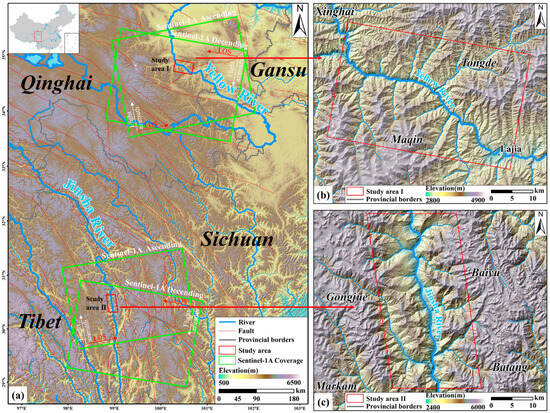
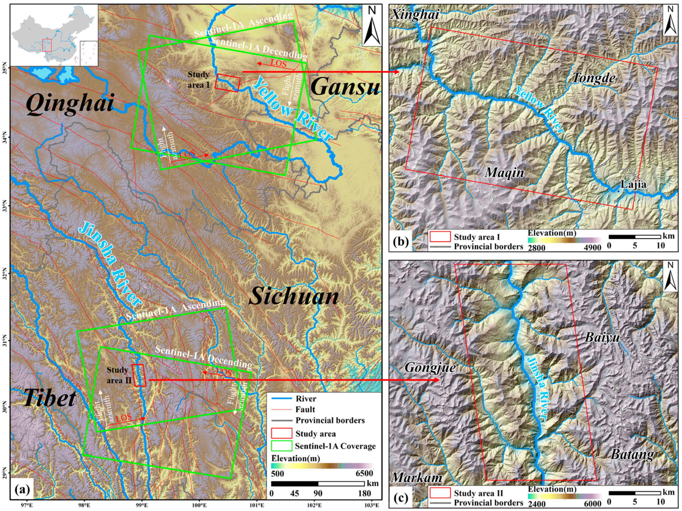
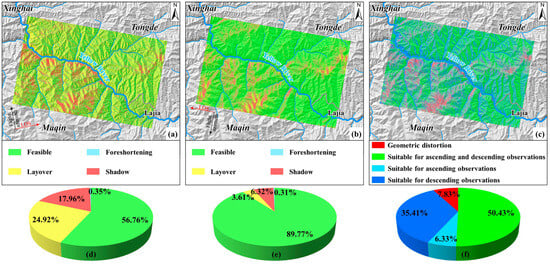
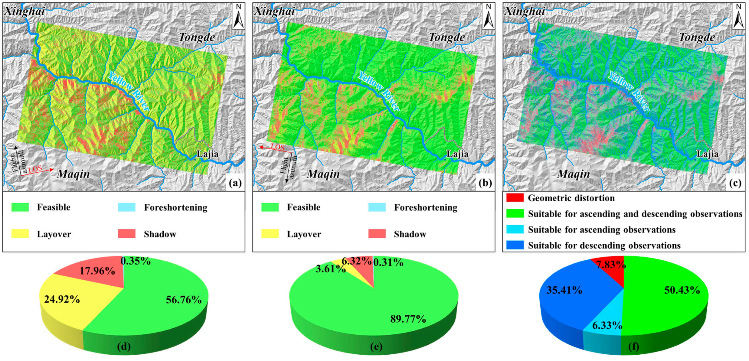
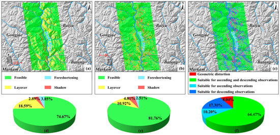
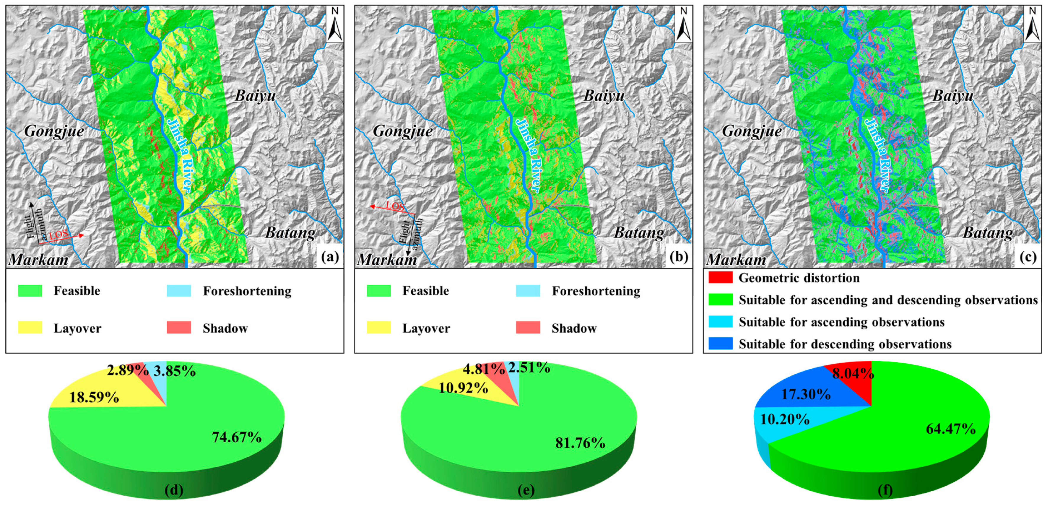
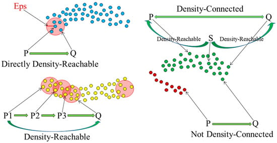
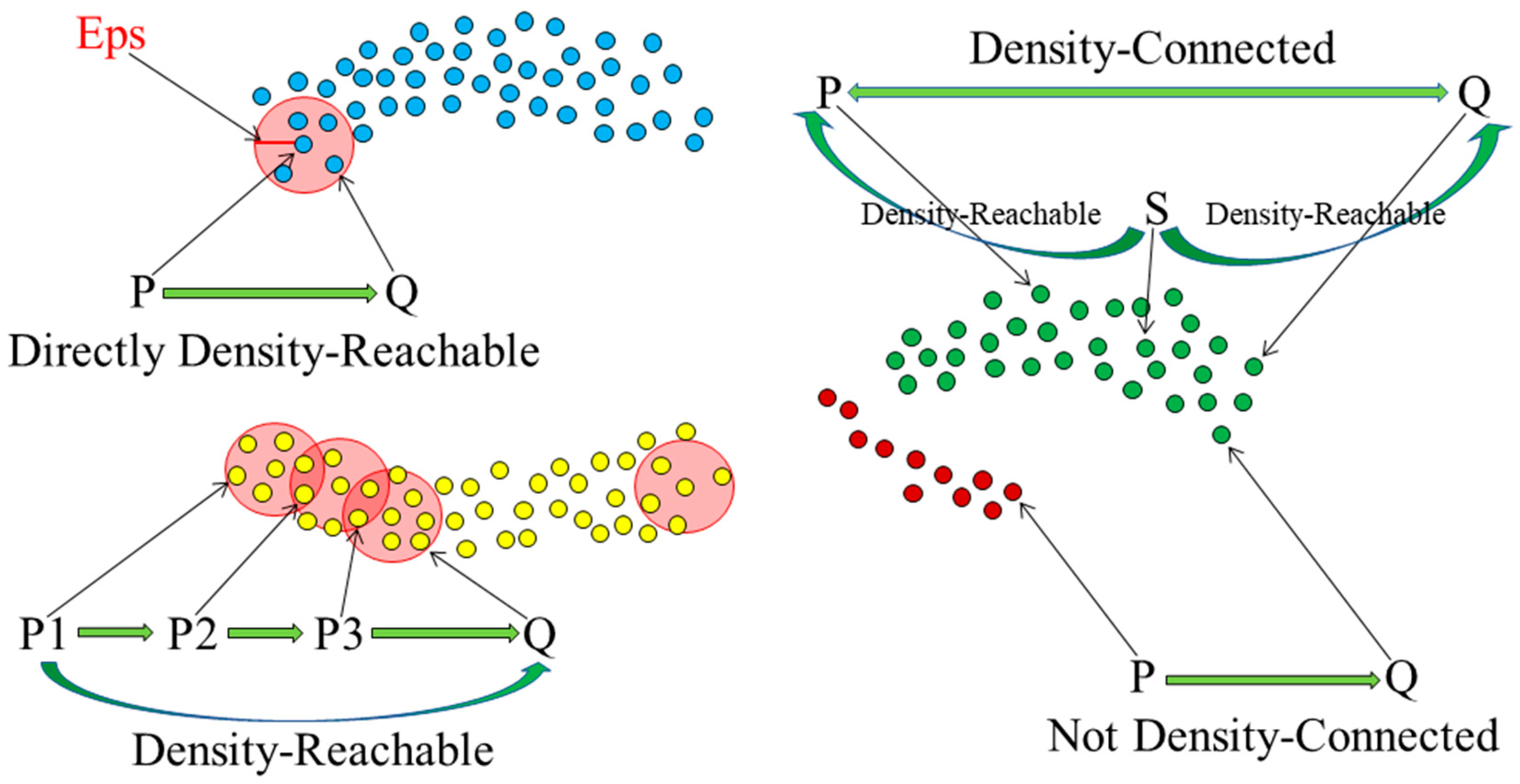
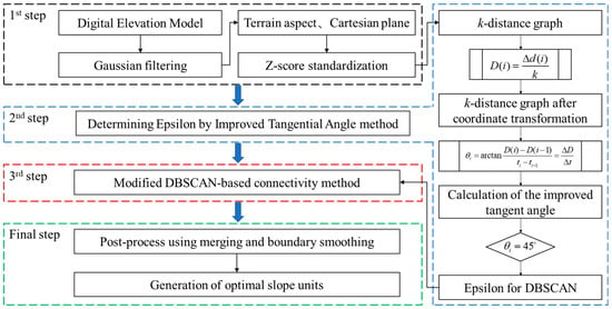
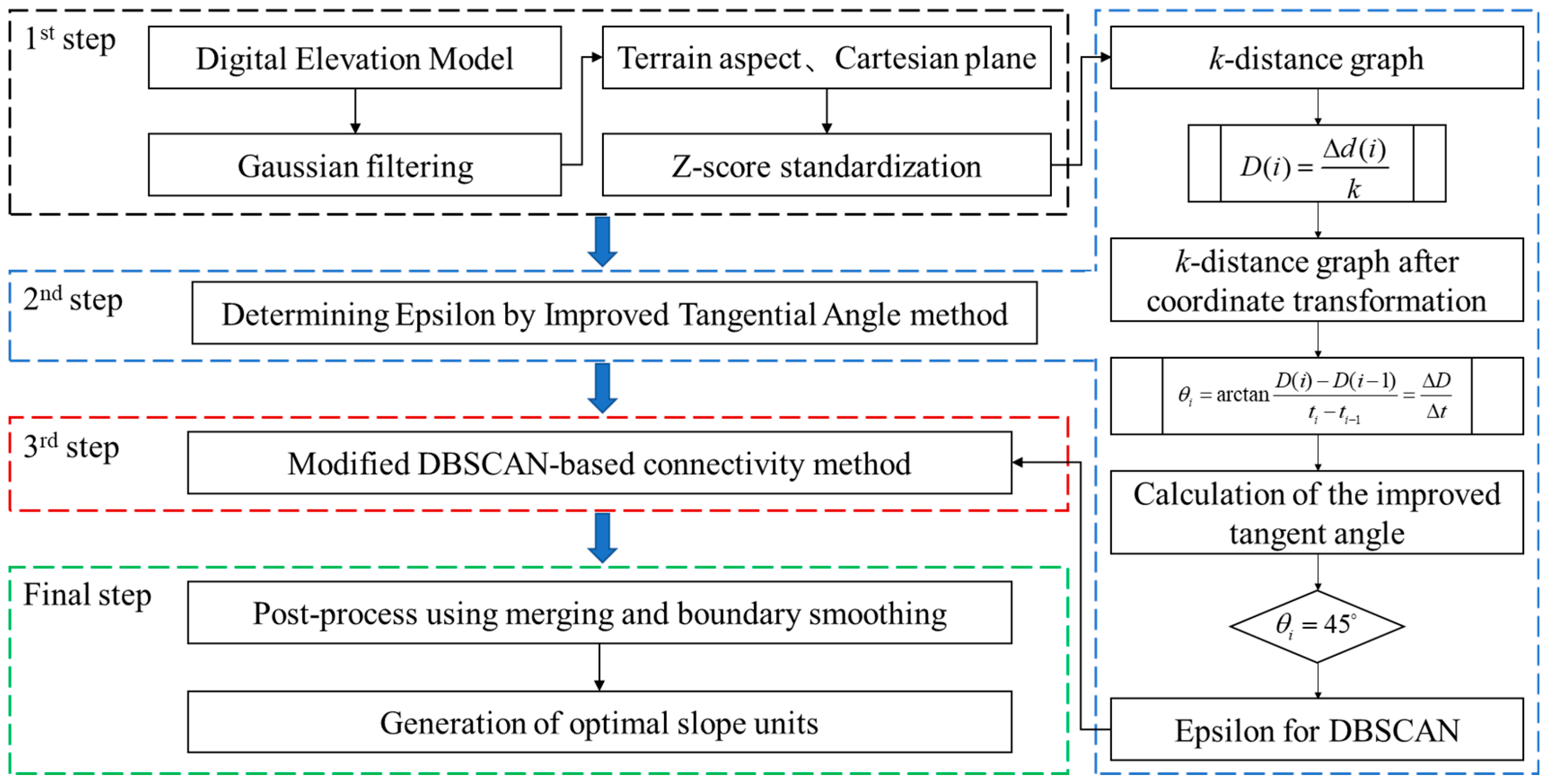
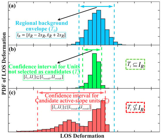
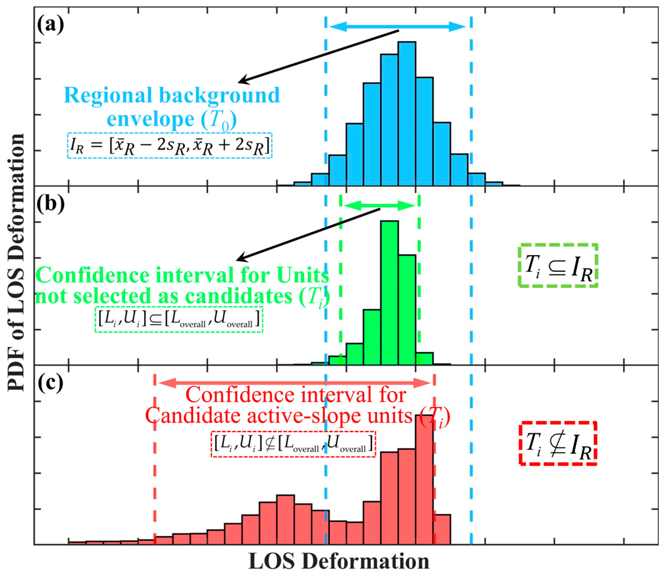
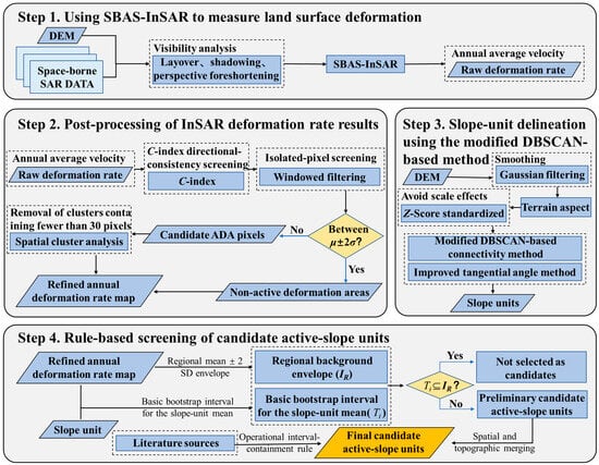
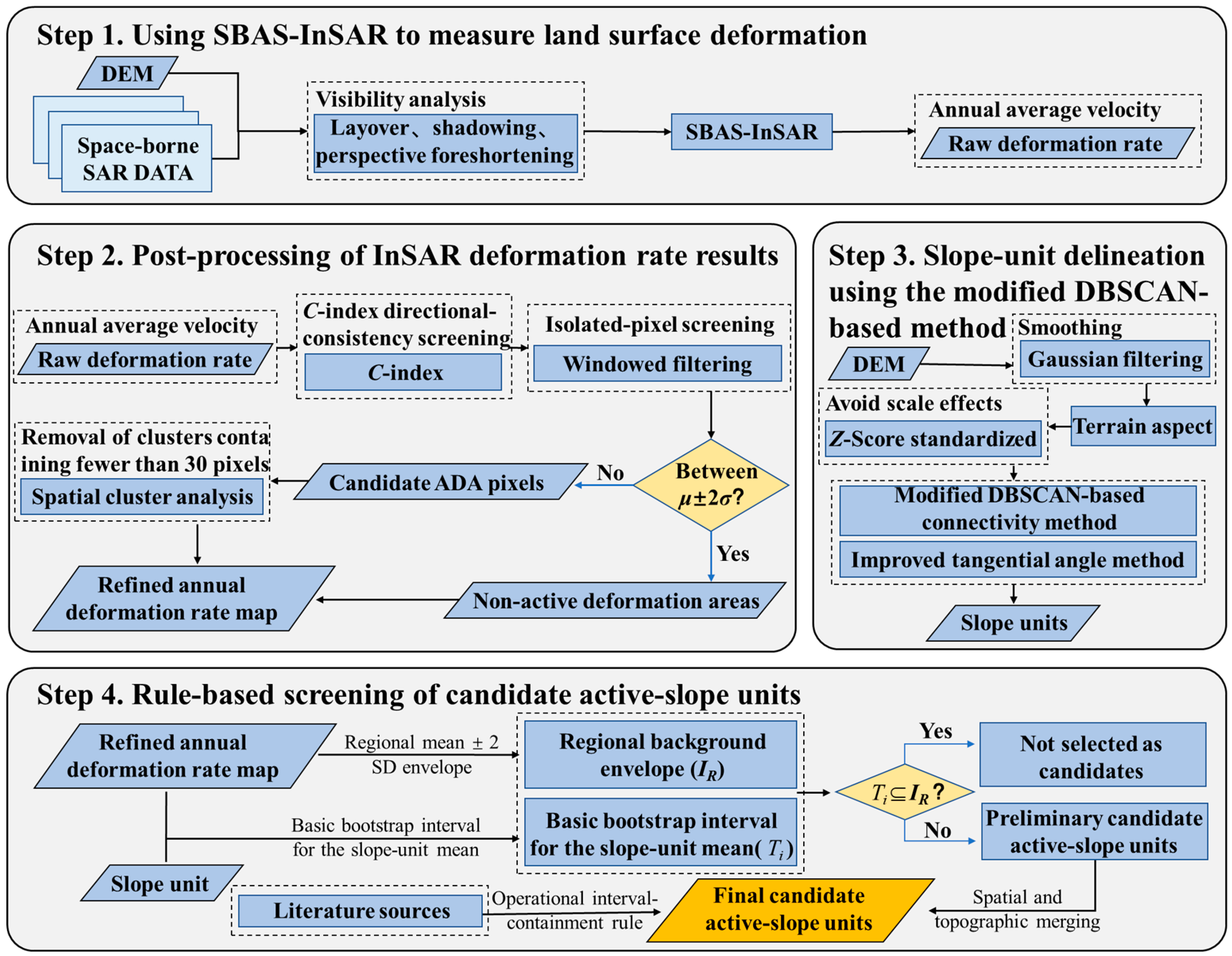
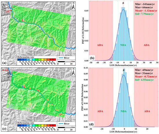
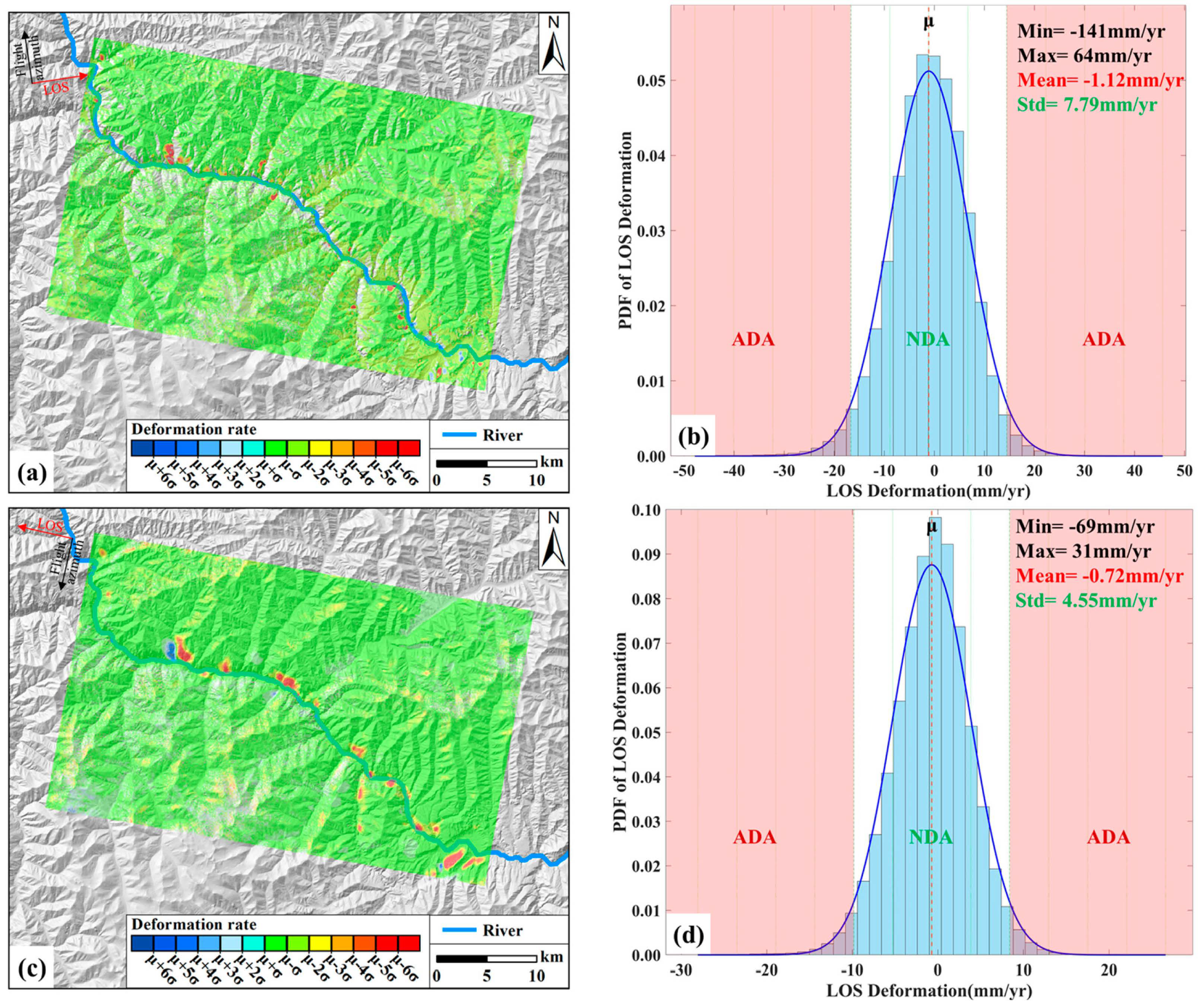
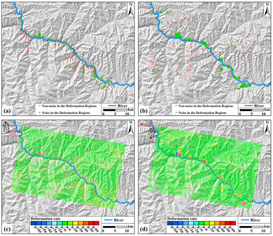
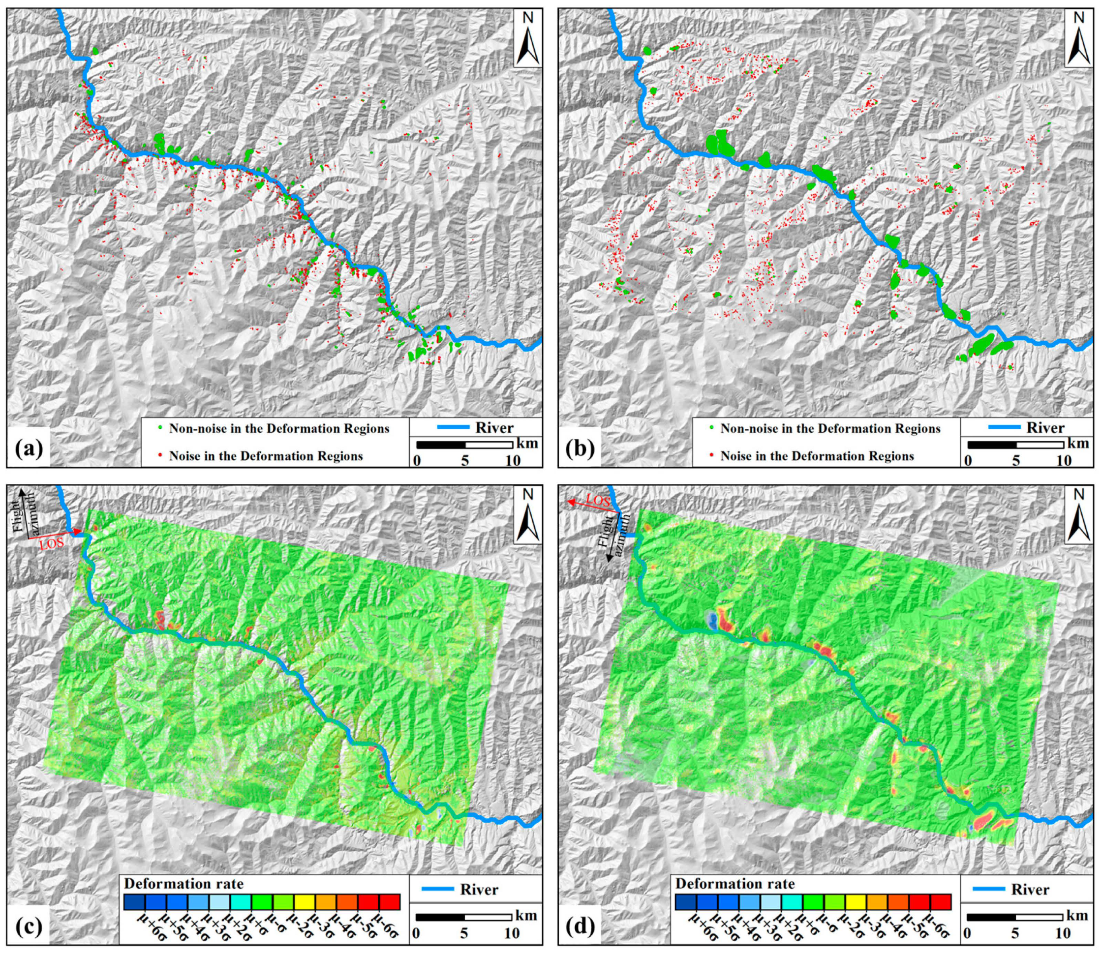
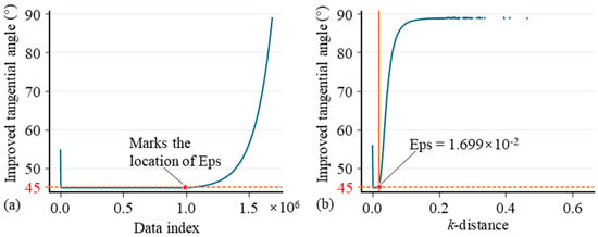
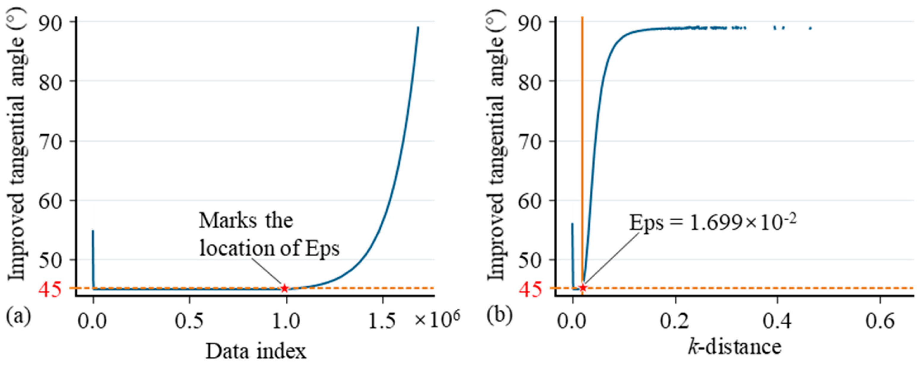
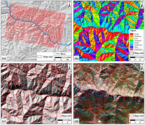
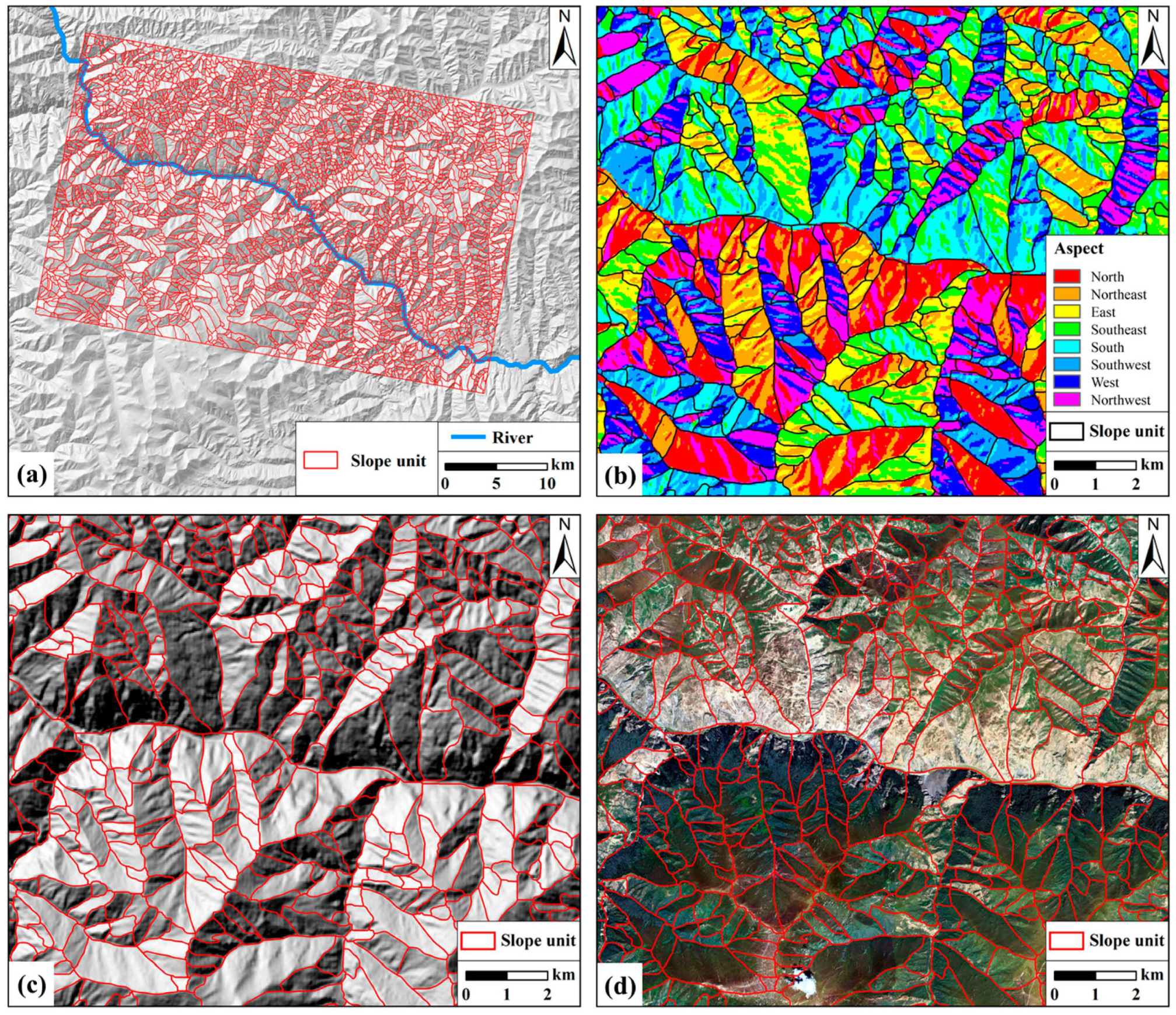
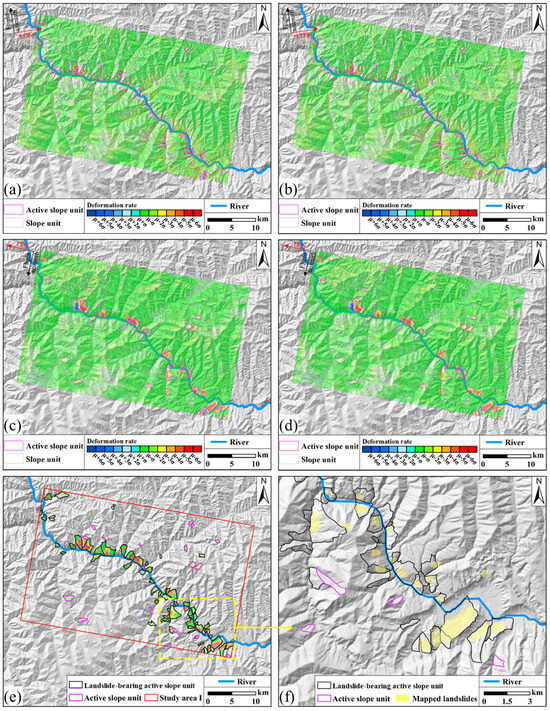
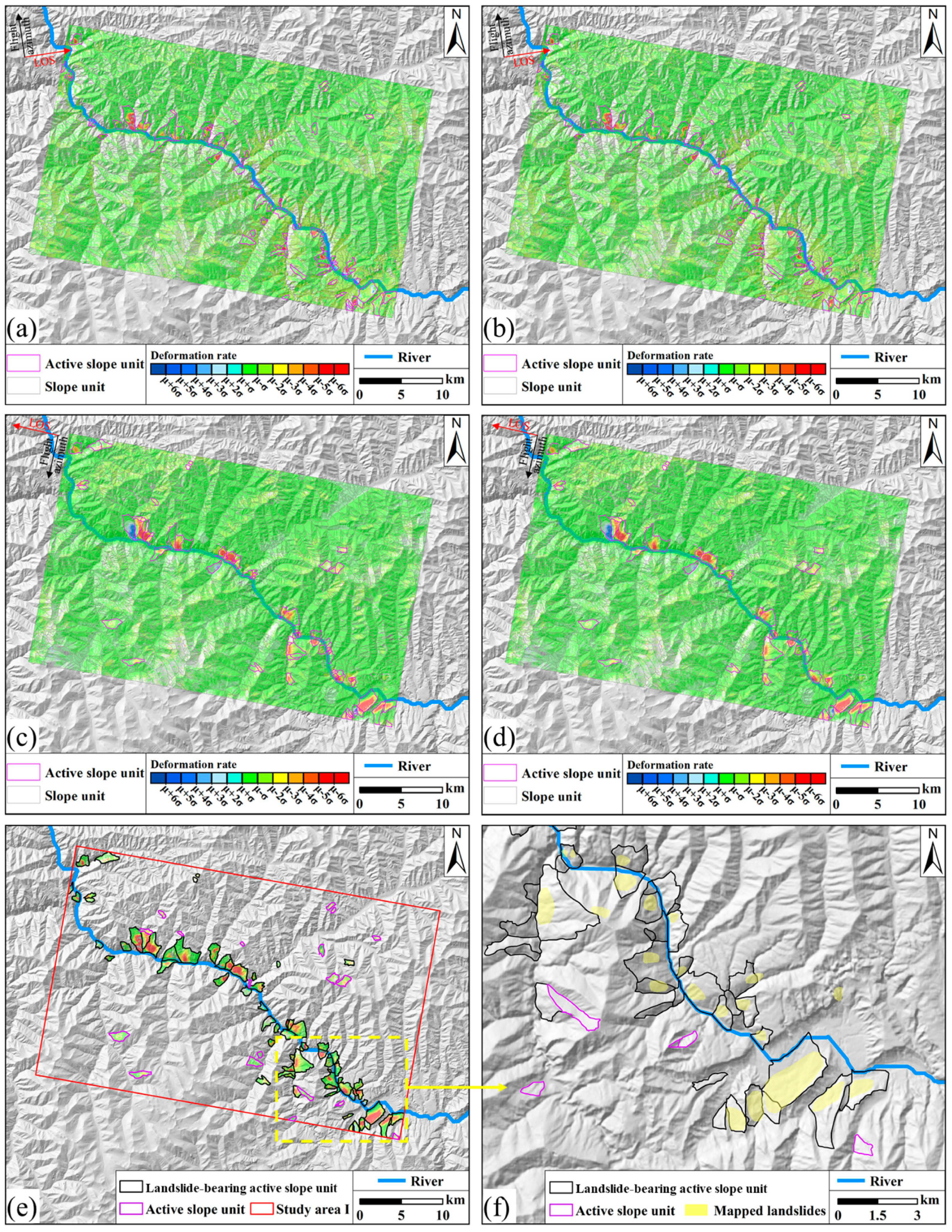
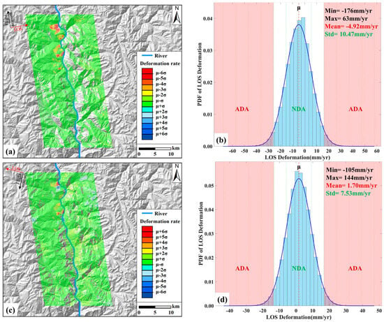
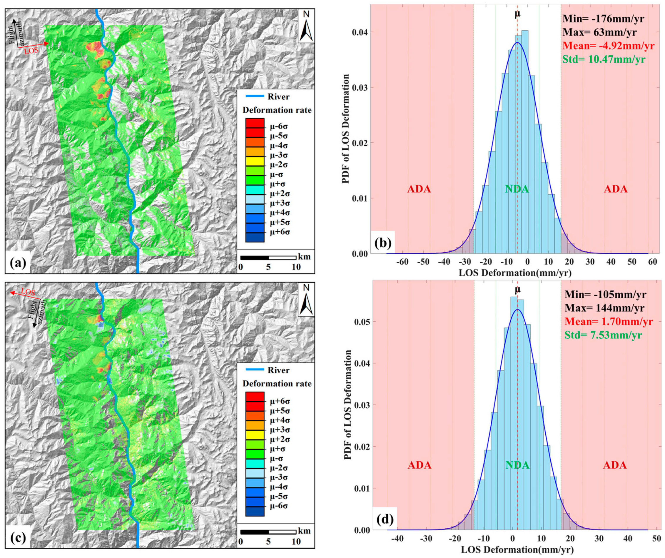
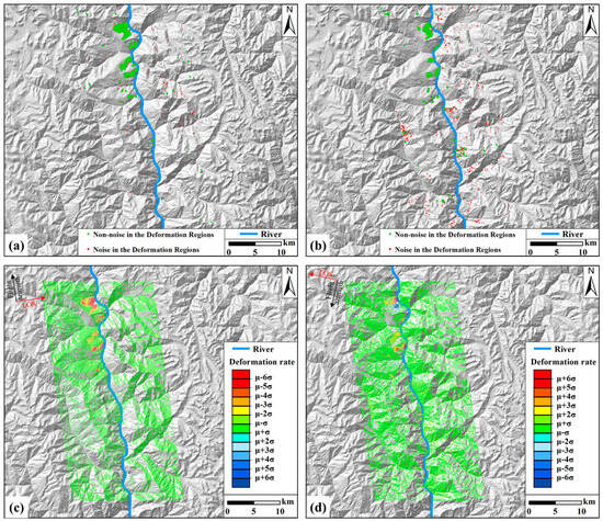
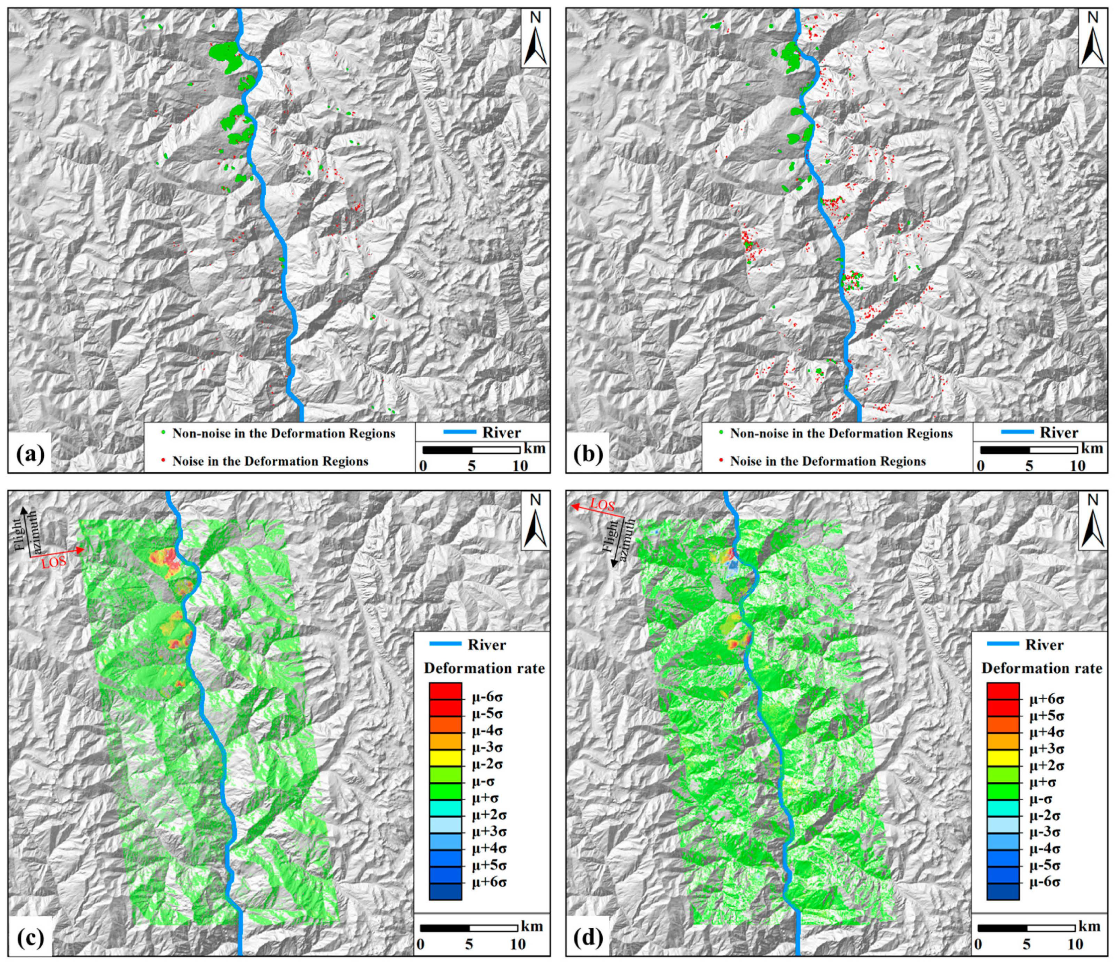
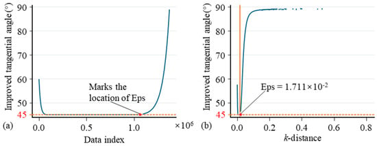
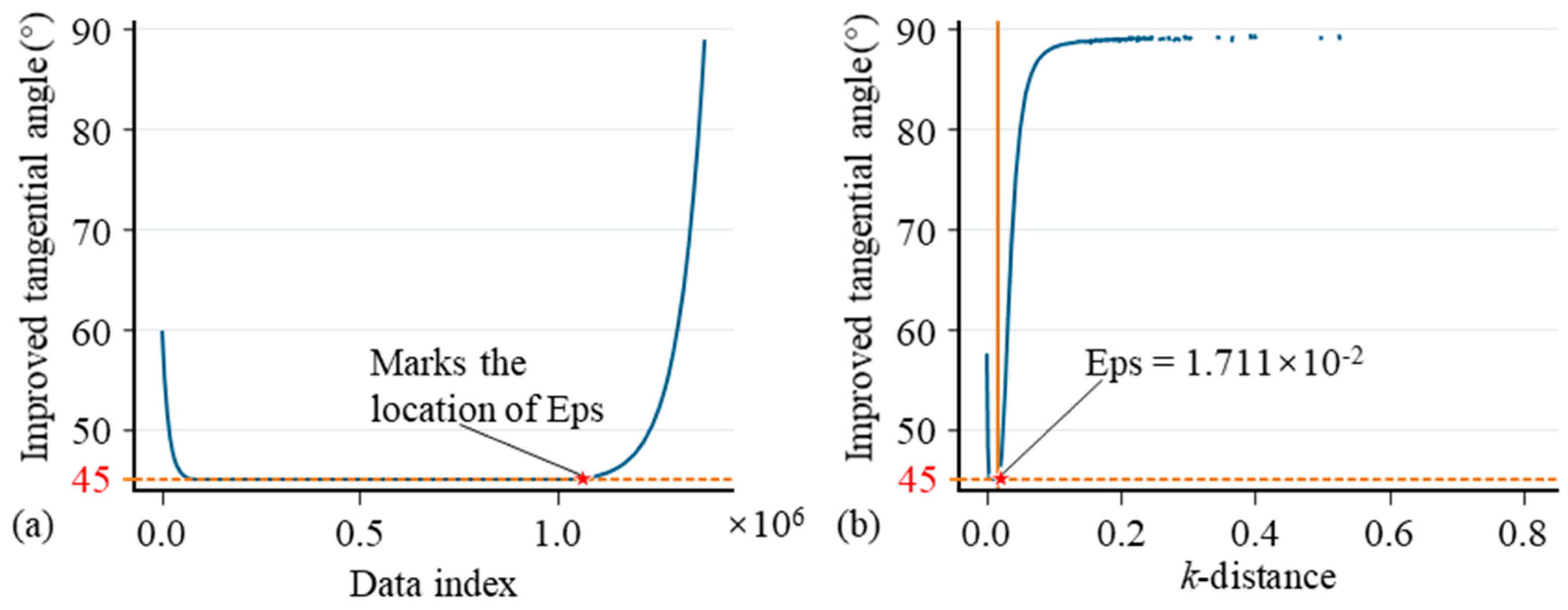
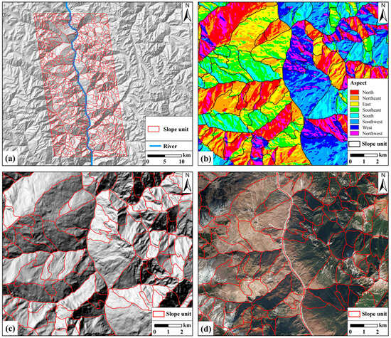
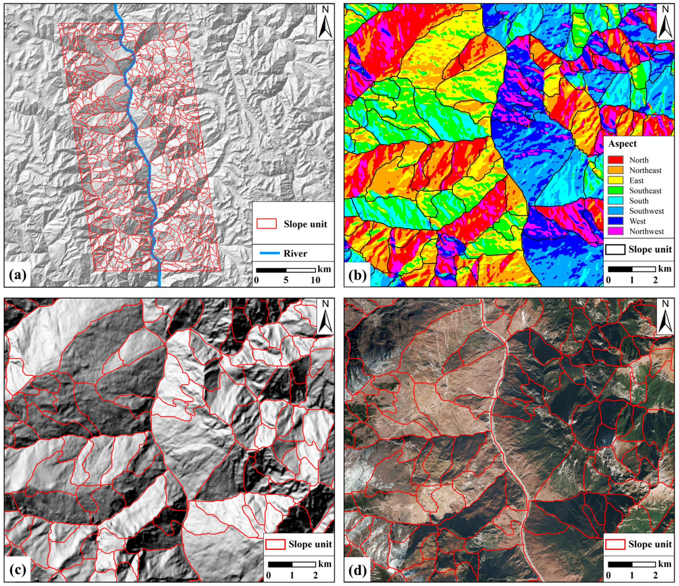
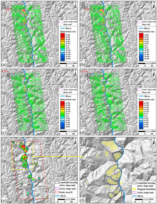
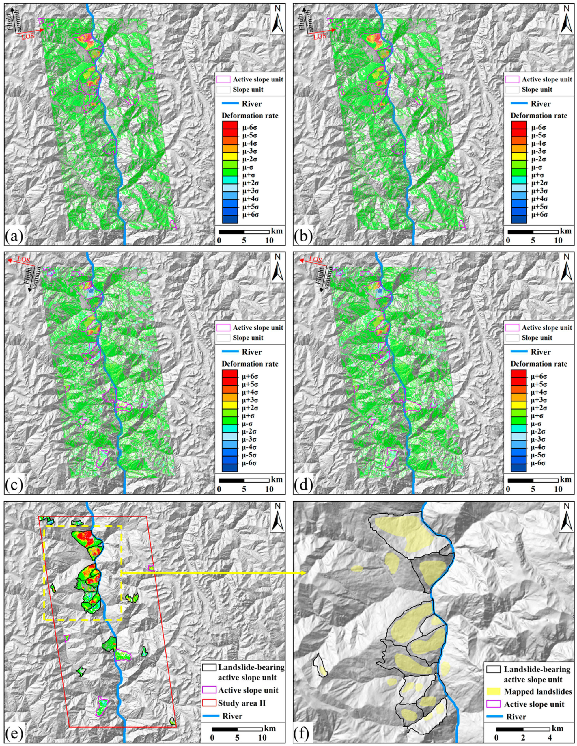

Disclaimer/Publisher’s Note: The statements, opinions and data contained in all publications are solely those of the individual author(s) and contributor(s) and not of MDPI and/or the editor(s). MDPI and/or the editor(s) disclaim responsibility for any injury to people or property resulting from any ideas, methods, instructions or products referred to in the content. |
© 2026 by the authors. Licensee MDPI, Basel, Switzerland. This article is an open access article distributed under the terms and conditions of the Creative Commons Attribution (CC BY) license.