Residual Diagnosis-Guided Abundance Correction for Blind Hyperspectral Image Unmixing

Highlights

What are the main findings?

•

Reconstruction error alone does not consistently reflect abundance accuracy, whereas structured residual descriptors provide more effective information for abundance correction than raw residuals.

•

Using only 1% reference abundances, RDAC reduces A-RMSE by 55.05%, 70.80%, and 59.63% relative to the initial UNMamba estimates on Jasper Ridge, Samson, and Urban, respectively. Substantial improvements are also obtained with an alternative NMF backbone.

What are the implications of the main findings?

•

Structured residual diagnosis enables refinement of an existing blind-unmixing solution without relearning the complete spectral-to-abundance mapping.

•

Results with UNMamba and NMF show that residual-guided abundance post-correction can be applied to different blind-unmixing initializations under limited reference supervision.

Abstract

Recent blind hyperspectral image unmixing methods have achieved effective spectral–spatial representation, yet the reliability of estimated abundances remains difficult to assess because errors in jointly estimated endmembers and abundances can compensate for each other. To address this issue, we propose Residual Diagnosis-Guided Abundance Correction (RDAC), a post-correction framework that preserves the initial abundance estimate as an anchor and characterizes its mismatch using structured reconstruction residuals. Abundance candidates are then combined with structured residual information, while only 1% reference abundances are used to learn the correction. RDAC was evaluated on the Jasper Ridge, Samson, and Urban datasets. With UNMamba as the primary blind-unmixing backbone, RDAC achieved A-RMSEs of 0.0229, 0.0175, and 0.0359, reducing the initial errors by 55.05%, 70.80%, and 59.63%, respectively. It also achieved the lowest mean A-RMSE among the compared methods on Jasper Ridge and Samson while remaining competitive on Urban. Further experiments showed that reconstruction error alone does not reliably indicate abundance accuracy. When applied to NMF, RDAC reduced A-RMSE by 80.45%, 89.25%, and 77.61% on the three datasets. The results indicate that structured residual diagnosis can support abundance correction under limited supervision, and the NMF experiment shows that the same correction framework can also be used with an alternative blind-unmixing backbone.

1. Introduction

Hyperspectral image unmixing resolves mixed-pixel spectra into material-specific signatures and their fractional contributions, enabling composition analysis below the sensor pixel scale. At typical imaging resolutions, the signal recorded for one pixel may combine several surface materials because distinct components coexist within the instantaneous field of view [1,2]. The resulting abundance fractions are therefore central to quantitative interpretations of material composition. Beyond unmixing, hyperspectral representations also support anomaly detection and cross-domain classification. Recent examples include dual-stream background modeling with anomaly suppression [3] and group-aware spectral perturbation consistency for cross-domain few-shot classification [4]. These applications further illustrate the need to account for spectral–spatial structure and unreliable observations.

Blind hyperspectral unmixing seeks to recover both endmembers and abundances directly from the observed image, but their joint estimation remains inherently ambiguous [5]. Geometric methods constrain the solution through simplex structures and minimum-volume criteria [6,7,8], matrix-factorization approaches introduce non-negativity, sparsity, or manifold regularization [9,10,11], and Bayesian formulations exploit statistical priors and spatial dependence [12,13,14]. Spatial coherence has also been incorporated directly into blind endmember–abundance estimation [15]. Deep-learning approaches have expanded this line of research [16] through autoencoder-based architectures [17,18], convolutional models [19], Transformer-based models [20,21], and, more recently, Mamba-based state-space architectures [22,23]. However, these advances improve the representation and optimization of the joint decomposition without eliminating the coupling between endmember and abundance estimation.

This coupling makes spectral reconstruction fidelity an incomplete measure of abundance reliability. Recent studies have recognized the need to refine endmembers and abundances separately [24], while experimental evidence indicates that lower reconstruction error does not necessarily correspond to higher abundance accuracy [25]. Because the observed spectrum is jointly determined by the estimated endmembers and abundances, errors in the two components can partially compensate for each other. As a result, different endmember–abundance combinations may yield similar reconstruction quality while producing different abundance estimates. A blind-unmixing solution with a low reconstruction error may therefore still contain systematic abundance bias.

Residual information has been used in different forms in hyperspectral unmixing, mostly within the original decomposition process. Spectral-variability models introduce scaling or perturbation terms to describe deviations from fixed endmembers [26,27,28,29,30,31,32], while nonlinear models account for departures from the linear mixing assumption [33,34]. Residual component analysis models unexplained spectral components jointly with the unmixing variables and uses their spatial structure to describe model mismatch [35]. Bundle-based methods address spectral variability by using multiple spectral representations for each material [36]. More recently, residual-guided weighted NMF has used reconstruction residuals to adjust the contributions of unreliable spectral bands and pixels during blind unmixing [37], while other work has modeled spectral variability through scaling factors and residual perturbations [38]. In these studies, residual or mismatch information is incorporated during unmixing and affects the estimation of abundances, endmembers, or additional residual terms. By comparison, the residual of an already obtained blind-unmixing result has received less attention as a source of information for subsequent abundance correction. Such residuals preserve information on spectral shape, magnitude, spatial distribution, and covariance that cannot be represented by a single reconstruction-error value.

Supervised and semi-supervised methods provide another way to improve abundance estimation. Supervised approaches learn the mapping from spectra to abundances using labeled or constructed samples [39,40,41,42], while semi-supervised methods introduce additional prior or labeled information into the unmixing process [43,44]. Nearly blind unmixing has also shown that a small number of labeled pixels can provide useful constraints [45]. In these methods, the reference information is generally used to estimate abundances directly or to guide the original decomposition. A different situation arises when a scene-specific blind-unmixing result is already available and only its abundance estimates need to be corrected.

RDAC is developed for this setting. It retains the initial abundance estimate as an anchor, uses structured residual descriptors to describe the current reconstruction mismatch, introduces abundance candidates to provide alternative correction cues, and learns the correction from a small set of reference abundances. The original blind-unmixing backbone remains unchanged. The experiments examine the relationship between reconstruction fidelity and abundance accuracy, the role of structured residual information in abundance correction, and the performance of RDAC with limited reference samples. Its use with an alternative blind-unmixing backbone is also evaluated.

2. Methods

2.1. Problem Definition and Overall Design

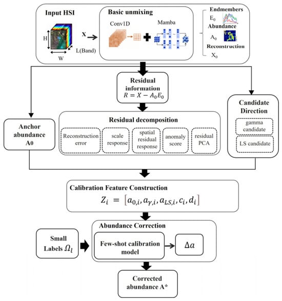
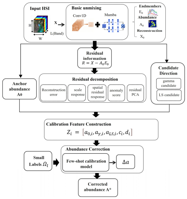
Given a target hyperspectral image, RDAC assumes that initial endmember and abundance estimates have already been obtained from a blind-unmixing model. The objective is not to repeat the full endmember–abundance decomposition, but to preserve the scene-specific structure learned by the blind-unmixing backbone and use a small set of reference abundances to correct systematic biases in its initial abundance estimates. Figure 1 illustrates the overall RDAC workflow.The pseudocode diagram of the specific algorithm is presented in Section 2.3.

Figure 1. Overall framework of the proposed Residual Diagnosis-Guided Abundance Correction (RDAC) method.

2.2. Residual Diagnosis-Guided Abundance Correction

For a target hyperspectral image X∈R^{N × L}, the blind unmixing backbone first outputs initial abundance estimate A₀∈^{N × P} and endmember estimate E₀∈R^{P × L}, where N, L, and P denote the numbers of pixels, spectral bands, and endmembers, respectively. The estimated endmembers E₀ are kept fixed during subsequent correction. The initial abundance A₀, after nonnegative normalization, retains material-composition and spatial-structure information learned from the full unlabeled image and is therefore used as the correction anchor. The reconstruction residual

R = X − A₀E₀

(1)

represents the spectral components that are not fully explained by the current endmember–abundance combination.

A scalar reconstruction RMSE summarizes only the overall residual magnitude, whereas abundance correction may depend on differences among pixels in fitting error, spectral shape, residual scale, and local spatial organization. Accordingly, the residual diagnostics are not designed to assign each descriptor to a unique physical perturbation. Instead, they provide complementary descriptions of the mismatch state associated with the current blind-unmixing solution.

The explicit diagnostic features include reconstruction error e_i, spectral angle θ_i, scale response S_i, local residual aggregation $l_i^{\mathit{agg}}$ and local residual outlier response $l_i^{\mathit{out}}$.

$$d_i=\left[e_i,{\theta }_i,S_i,l_i^{\mathit{agg}},l_i^{\mathit{out}}\right]$$

(2)

These quantities are combined into an explicit diagnostic vector. e_i and θ_i characterize numerical and spectral-shape discrepancies, respectively, while denotes S_i the overall magnitude deviation between the observed and reconstructed spectra. Spatial responses are derived from the pixel-wise reconstruction error map: $l_i^{\mathit{agg}}$ uses neighborhood averaging to characterize spatially continuous high-residual structures, whereas $l_i^{\mathit{out}}$ estimates the local background using neighborhood statistics and measures positive residual deviations from the surrounding region. Reflect padding is applied at image boundaries. To reduce the influence of extreme values, S_i, $l_i^{\mathit{agg}}$ and $l_i^{\mathit{out}}$ are normalized using their respective percentile ranges and subsequently clipped.

Some mismatch patterns may not be fully captured by the explicit diagnostic vector d_i. RDAC therefore applies principal component analysis directly to the reconstruction residuals and retains the leading q principal components. The PCA basis is estimated from the residuals of the entire unlabeled target image without using reference abundances. The corresponding coefficient vector c_i provides a compact representation of the dominant residual covariance structure and complements the interpretable descriptors in d_i.

Even with this diagnostic representation, the residual state alone does not determine how the abundance estimate should be adjusted. The direction and magnitude of the correction therefore need to be inferred from additional correction cues and limited reference information. RDAC further introduces two abundance candidates to provide candidate correction directions. The residual descriptors are not assumed to have a one-to-one correspondence with specific abundance errors. Instead, they provide complementary descriptions of the current mismatch state, while the correction direction and magnitude are learned from the limited reference abundances.

The first is the Gamma candidate. The results of deep blind unmixing may result in an overly smooth or weak response dispersion, so nonlinear redistribution from the A0 itself provides an abundance steering direction without altering the endmember semantics:

$$a_{\gamma ,i,k}={\displaystyle \frac{a_{0,i,k}^{\gamma }}{{\displaystyle {\sum }_{j=1}^P}{a}_{0,i,j}^{\gamma }}}\gamma >1$$

(3)

a_γ,i is introduced as a constrained perturbation of the initial abundance estimate rather than as an independent estimator. After normalization, it preserves the abundance constraints and component ordering while continuously adjusting the concentration of the abundance distribution. It therefore provides a simple and physically admissible correction direction derived from A₀, without modifying the endmembers or introducing additional spectral fitting.

The second candidate, denoted by a_LS,i, is obtained by re-estimating the abundances under the fixed endmembers E₀ using constrained least squares with non-negativity and abundance-sum-to-one constraints. It represents the abundance configuration preferred by spectral fitting under the current fixed endmembers.

$$a_{\mathit{LS},i}={\mathit{argmin}}_{a\in {\mathbb{R}}^{1\times P}}\left({\left|\left|x_i-a{E}_0\right|\right|}_2^2\right) s.t. a\ge 0 a{1}_p=1$$

(4)

Thus, a_γ,i and a_LS,i provide possible correction directions from two perspectives: redistribution guided by the structure of the initial abundances and adjustment guided by spectral fitting with the fixed endmembers. Together, they form the candidate abundance set.

Because the appropriate correction direction and magnitude may vary across pixels, RDAC combines the above information into a pixel-level correction feature vector:

$$z_i=\left[a_{0,i},{a_{\gamma ,i},a_{\mathit{LS},i},c}_i,d_i\right]$$

(5)

Here, a_0,i serves as the correction anchor, a_γ,i and a_LS,i provide correction candidate directions, and c_i and d_i describe the current residual state.

A small number of reference abundances are then used to learn the correction of the existing prediction rather than to relearn the complete spectral-to-abundance mapping. For a labeled training pixel, the supervised target is defined as

$$∆a_i=a_i^{\mathit{ref}}-a_{0,i}$$

(6)

Reference abundances are used only to construct the correction targets for the labeled training pixels. They are not used to compute the residual diagnostics, Residual PCA basis, or candidate abundance estimates. To reduce overfitting under few-sample conditions and avoid attributing the improvement to a complex predictor, RDAC uses an L2-regularized ridge regressor to learn the relationship between z_i and ∆a. The regularization coefficient is fixed at λ = 10⁻². The regressor is fitted only on the labeled training pixels and is subsequently applied to the remaining pixels to predict their abundance corrections. The purpose of the corrector is therefore to learn which correction direction should be used and how large the correction should be under the current diagnostic state, rather than to reconstruct the complete abundance mapping from scratch. Because E₀ is kept fixed, RDAC cannot explicitly separate abundance errors from errors caused by inaccurate endmember estimation. In some cases, abundance correction may partially compensate for endmember mismatch. Therefore, the corrected abundance should be interpreted as a refinement under the current fixed-endmember model rather than as a complete correction of all sources of unmixing error.

For an unlabeled pixel, the corrector predicts

$$\widehat{∆a_i}=f_{\theta }\left(z_i\right)$$

(7)

and the final abundance is obtained by applying the predicted correction to A₀

A^* = Π(A₀ + F(Z))

(8)

where Π(*) denotes non-negative truncation followed by normalization onto the abundance simplex. Overall, RDAC preserves the scene information captured by blind unmixing and restricts limited supervision to learning corrections to existing predictions, thereby converting full abundance relearning into a lightweight post-correction task.

2.3. Algorithm Summary

To facilitate understanding of the proposed method, the main steps and implementation details are summarized in Algorithm 1.

Algorithm 1. Residual Diagnosis-Guided Abundance Correction (RDAC)
Input: Target-scene spectra X and spatial dimensions; Initial abundances A0 and fixed endmembers E0; Labeled training indices T and reference abundances Aref, T; PCA dimension q, ridge parameter λ, and exponent γ; Diagnostic settings θ. Output: Corrected abundances Acorr.
1:	Stage A: Residual diagnosis
2: 3: 4:	Compute the initial reconstruction and residual matrix:   $\widehat{X}$ ← A0E0   R ← X − $\widehat{X}$
5: 6:	Compute the pixel-wise reconstruction mismatch:   $e_i\leftarrow \sqrt{{\displaystyle \frac{1}{L}}{\displaystyle {\sum }_{\mathcal{l}=1}^L} R_{i\mathcal{l}}^2}$
7: 8:	Estimate the spectral scale ratio:   ${\rho }_i\leftarrow {\mathit{Clip}}_{\Theta }\left({\displaystyle \frac{⟨{\mathit{X}}_i,{\hat{\mathit{X}}}_i⟩}{\Vert {\hat{\mathit{X}}}_i{\Vert }_2^2+\epsilon }}\right)$
9: 10: 11:	Compute spatial statistics of the mismatch map:   m ← LocalMedianθ(e)     u ← LocalMeanθ(e)
12: 13: 14: 15: 16:	Construct complementary mismatch descriptors:   s ← PercentileNormalizeθ(|log(ρ + ε)|)   v ← PercentileNormalizeθ(PositivePart(u − median(u)))   a ← PercentileNormalizeθ(PositivePart(e − m))   r ← Clipθ(wss + wvv + waa)
17: 18:	Assemble the explicit diagnostic features:   D ← [PercentileNormalizeθ(e), PercentileNormalizeθ(ρ), s, v, a, r]
19:	Stage B: Residual PCA
20: 21: 22:	Center the residuals using all target-scene pixels:   μR ←MeanRows(R)   Rc←R − μR
23: 24:	Estimate the residual covariance matrix:   C ← Covariance(Rc)
25: 26:	Extract the leading q eigenvectors:   Bq ← LeadingEigenvectors(C, q)
27: 28:	Compute residual PCA features:   P ← RcBq
29:	Stage C: Candidate generation and feature construction
30: 31: 32:	Construct candidate abundances:   Aγ ← Normalize(SafeClip(A0)^γ)   ALS ← Normalize(XE0†)
33: 34:	Concatenate the RDAC features:   Φ ← [A0, Aγ, ALS, ALS − A0, P, D]
35:	Stage D: Supervised abundance correction
36: 37: 38:	Estimate feature standardization statistics from ΦT only.  Standardize Φ using these training statistics.  Append an intercept column to obtain Z.
39: 40:	Construct the training correction targets:   YT ← Aref,T − A0,T
41: 42:	Fit the ridge corrector:   W ← argminW${\Vert Z_{T}W - Y_T\Vert }_F^2$ + λ${\Vert W_{\mathit{feature}}\Vert }_F^2$
43: 44:	Predict abundance corrections:   ΔA ← ZW
45: 46:	Obtain the corrected abundances:   Acorr ← Normalize(A0 + ΔA)
47:	Return Acorr.

3. Experimental Settings and Results

The experiments focused on three key issues: first, whether blind-unmixing results exhibit a mismatch between good spectral reconstruction and inaccurate abundance estimates; second, whether structured residuals could provide diagnostic information related to the correction of abundance; third, whether RDAC can provide stable post-correction gains under limited reference supervision and remain robust to sample allocation, parameter settings, and changes in the initial blind-unmixing backbone.

3.1. Datasets

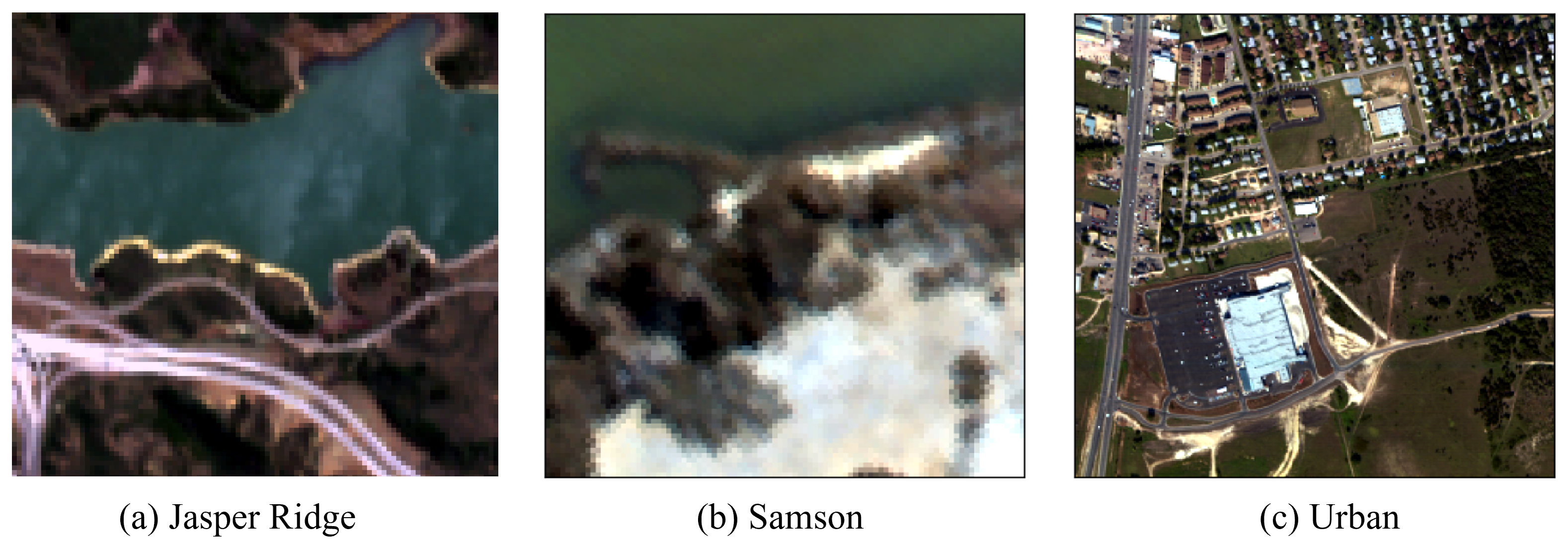
Experiments were conducted on three real hyperspectral datasets with reference abundances (as shown in Figure 2): Jasper Ridge, Samson, and Urban. The Jasper Ridge dataset contains 100 × 100 pixels, with 198 valid spectral bands and four major endmember classes; the Samson dataset contains 95 × 95 pixels, with 156 spectral bands and three major endmember classes; and the Urban dataset contains 307 × 307 pixels, with 162 valid spectral bands and four major endmember classes. The datasets were obtained from publicly available hyperspectral unmixing benchmarks, and the initial blind-unmixing estimates were generated using the corresponding backbone methods. Abundance estimation performance was evaluated using A-RMSE, with lower values indicating more accurate abundance estimates.

Figure 2. Color images of the experimental datasets.

Figure 2. Color images of the experimental datasets.

3.2. Experimental Setup

The initial blind-unmixing solution was obtained using the public implementation of UNMamba. Its abundance estimates A₀ and endmember estimates E₀ were directly reused without retraining the backbone, and E₀ remained fixed during post-correction. NMF was used only for the subsequent cross-backbone evaluation.

In the main experiment, 1% of the pixels with reference abundance labels were randomly selected as the training set for abundance correction, while the remaining pixels were used for testing. The experiment was repeated using five different random seeds. To avoid using test ground truth to determine the correspondence between estimated and reference abundance channels, channel alignment was performed using only the training pixels. All possible channel permutations were evaluated on the training set, and the permutation yielding the lowest abundance error was fixed and subsequently applied to the test pixels. Test reference abundances were not involved in determining the channel correspondence. For each random seed, all comparison methods used the same training–test split.

The main RDAC parameters were fixed before evaluation, with the Residual PCA dimension q = 8 and ridge regularization coefficient λ = 10⁻² shared across all datasets. For the spatial residual diagnostics, a 5 × 5 median filter was used to estimate the local background for the outlier response, while an 11 × 11 mean filter was used to characterize locally aggregated residual structures, with reflect padding applied at image boundaries. The Gamma exponent γ was set to 1.45, 1.10, and 1.50 for Jasper Ridge, Samson, and Urban, respectively. These dataset-specific values were determined using only the training reference abundances and were fixed before evaluation on the corresponding test pixels. All target-image pixels were used to construct residual diagnostics and the Residual PCA basis, whereas only the training reference abundances were used to fit the correction model. Test reference abundances were not used for feature construction, parameter selection, or model training.

3.3. Reconstruction–Abundance Relation

To examine whether spectral reconstruction quality reliably reflects abundance accuracy, we analyzed reconstruction and abundance errors from pixel-wise and spatial perspectives. Pearson and Spearman coefficients were used to quantify their linear and rank-order associations, while the corresponding error maps were compared to assess their spatial consistency. We also examined whether further improvements in reconstruction fidelity were accompanied by corresponding reductions in abundance error.

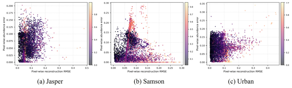
As shown in Table 1, reconstruction error and abundance estimation error exhibit only weak-to-moderate correlations across the three datasets. In particular, the Pearson coefficients for Samson and Urban and the Spearman coefficient for Urban are close to zero, indicating little linear or monotonic association in these cases. Overall, lower reconstruction error does not necessarily imply lower abundance error, suggesting that reconstruction fidelity alone is insufficient to characterize abundance reliability.

Table 1. Correlation between reconstruction error and abundance error.

Dataset	Pearson r	Spearman ρ
Jasper Ridge	0.3101	0.3205
Samson	0.0451	0.2049
Urban	0.0833	0.0257

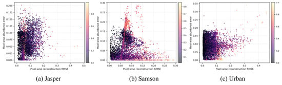
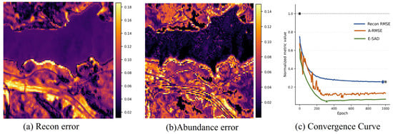
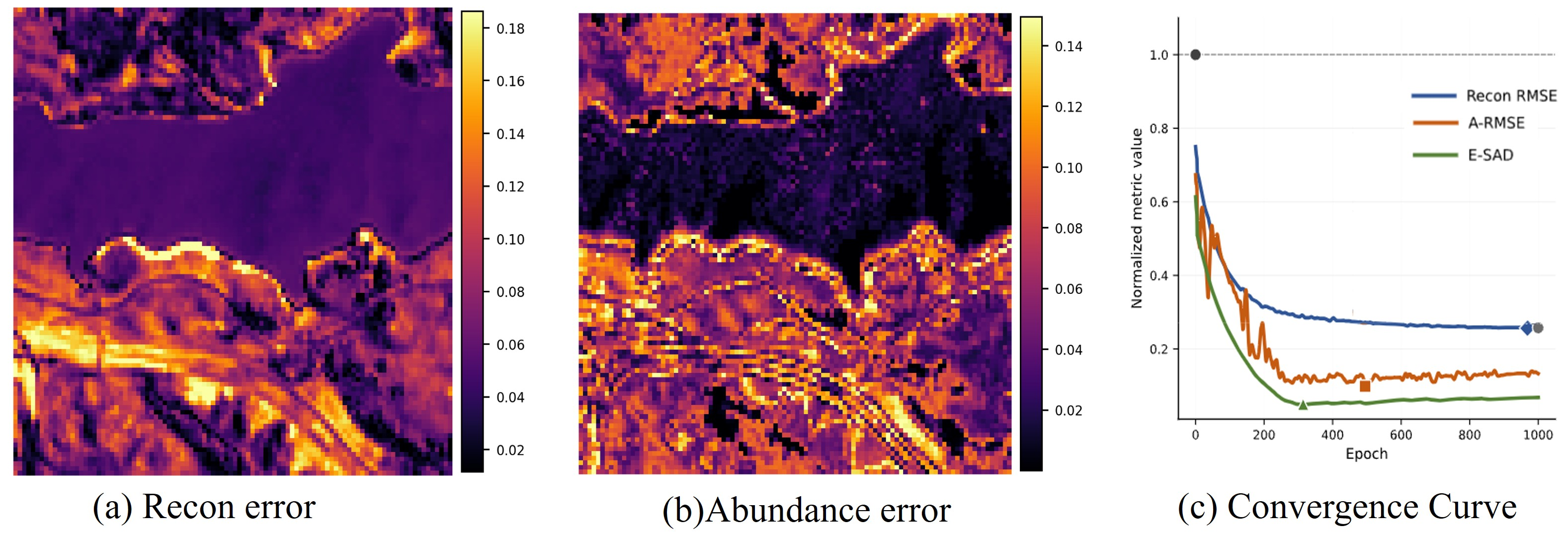
Figure 3 shows that pixels with similar reconstruction errors can exhibit markedly different abundance estimation errors. Figure 4 further shows that some spatial regions with relatively low reconstruction errors still exhibit pronounced abundance errors, and the spatial distributions of the two errors do not fully coincide. Further reductions in reconstruction error do not always lead to lower abundance estimation error, even when training is continued. These results indicate that spectral reconstruction quality and abundance estimation accuracy are related but not equivalent. Reconstruction error can therefore be used to assess spectral fit, but it should not be treated as a direct measure of abundance reliability.

Figure 3. Scatter plots of reconstruction error versus abundance error.

Figure 4. Spatial distributions of reconstruction error, abundance error, and convergence behavior.

Spatial distributions of reconstruction error, abundance error, and convergence behavior.The first two panels show the spatial distributions of the corresponding pixel-wise metric values, while the third panel illustrates the evolution of normalized reconstruction RMSE (Recon RMSE), abundance RMSE (A-RMSE), and endmember spectral angle distance (E-SAD) over training epochs. The horizontal dashed line indicates the normalized initial reference value (1.0). The diamond, square, and triangle markers indicate the epochs at which Recon RMSE, A-RMSE, and E-SAD reach their respective minimum values, respectively.

3.4. Controlled Perturbation Experiments

3.4.1. Diagnostic Responses

To examine whether reconstruction residuals contain structured information associated with different mismatch states, we considered three controlled perturbations: scale variation, local endmember spectral-shape variability, and sparse spectral anomalies. The corresponding perturbation strengths were set to 0.38, 0.16, and 0.26, respectively, with anomalous pixels accounting for approximately 0.8% of the image. These settings were chosen to generate clearly observable mismatch responses without substantially altering the dominant material-composition structure of the original scene. Under these controlled conditions, the scale response, Residual PCA response, and local anomaly response were computed and compared.

Table 2 shows that the scale response, Residual PCA response, and local anomaly response exhibit their strongest responses under their corresponding target perturbations, while each diagnostic response also shows some cross-sensitivity. These results indicate that different mismatch conditions produce partially distinguishable response patterns in the structured residual representation.

Table 2. Normalized diagnostic response matrix under controlled perturbations.

Injected Perturbation	Scale Score	Residual PCA Score	Anomaly Score
scale	1	0	0.222
variability	0.807	1	0.272
anomaly	0	0.878	1

3.4.2. Abundance Correctability Under Controlled Perturbations

Differences in diagnostic responses under controlled perturbations alone do not show whether the corresponding mismatch states are associated with correctable abundance errors. Therefore, we further performed auxiliary correction analyses for the three perturbation types. These procedures are not part of the formal RDAC inference process, but are used to examine whether the diagnosed mismatch states contain correction-relevant information.

As shown in Figure 5, Figure 6 and Figure 7 the three perturbation types produce different responses in the structured residual descriptors.For scale perturbations, the estimated scale response was used to compensate the observed spectra before re-estimating abundances with fixed endmembers. For endmember variability, target-supervised abundance correction was evaluated on the isolated variability regions to assess its ability to reduce systematic abundance errors. For spectral anomalies, high-risk pixels were identified using the local anomaly response, replaced with neighborhood median spectra, and then re-estimated. Because different correction strategies were used, the results are therefore used to assess error correctability under each mismatch condition rather than to compare the three correction strategies.The corresponding results are summarized in Table 3.

Figure 5. Controlled illumination-scale perturbation and abundance correction.

Figure 5. Controlled illumination-scale perturbation and abundance correction.

Figure 6. Controlled endmember-variability perturbation and abundance correction.

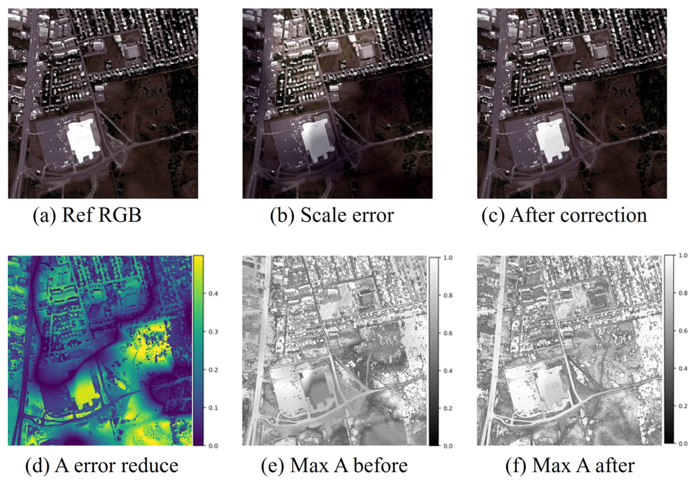
Figure 6. Controlled endmember-variability perturbation and abundance correction.

Figure 7. Controlled spectral-anomaly perturbation and abundance correction.

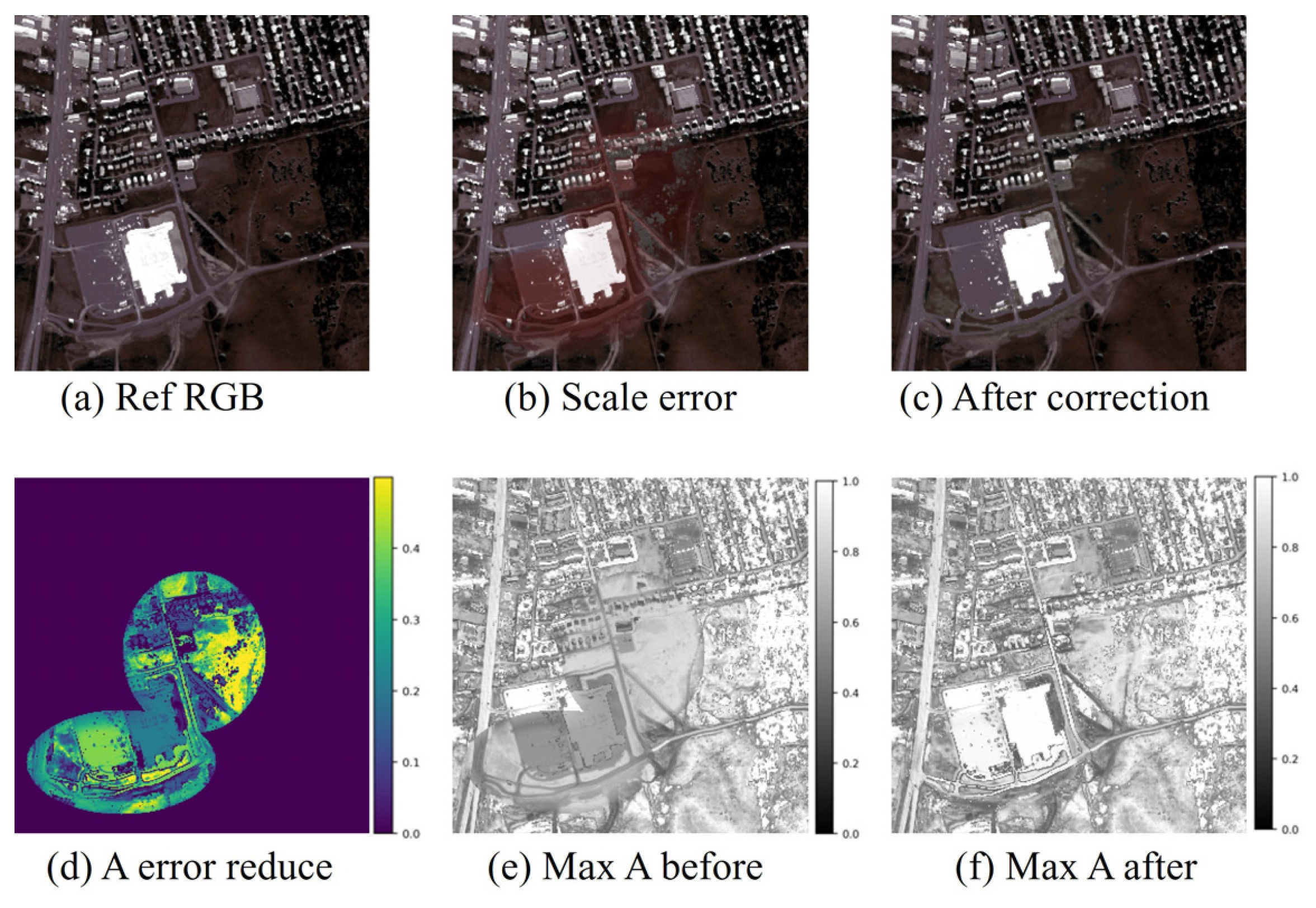
Figure 7. Controlled spectral-anomaly perturbation and abundance correction.

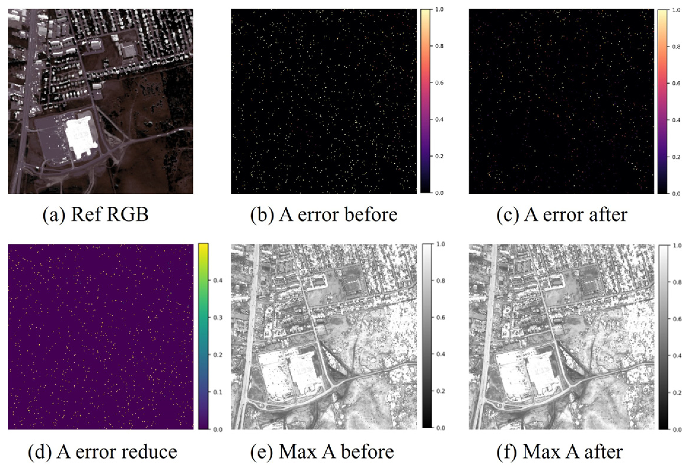
Table 3. Auxiliary abundance correction analysis.

Disturbed Area	Before Correction A-RMSE	After Correction A-RMSE	Relative Improvement
Light scale area	0.1963	0.0569	71.03%
Endmember variability region	0.3160	0.1114	64.75%
Spectral anomaly candidate region	0.3448	0.1551	55.02%

Table 3. Auxiliary abundance correction analysis.

Disturbed Area	Before Correction A-RMSE	After Correction A-RMSE	Relative Improvement
Light scale area	0.1963	0.0569	71.03%
Endmember variability region	0.3160	0.1114	64.75%
Spectral anomaly candidate region	0.3448	0.1551	55.02%

Together with the diagnostic response results above, these findings show that different controlled mismatches not only produce distinguishable patterns in the structured residual representation, but are also associated with abundance errors that can be effectively reduced through targeted correction. It should be emphasized that these results do not imply that any single diagnostic score can directly determine the true direction or magnitude of abundance correction. Rather, they indicate that the mismatch states characterized by structured residuals are related to correctable abundance errors, providing a basis for RDAC to learn the specific correction from a small number of reference abundances.

3.5. Real-Scene Experiments

3.5.1. Spatial Analysis of Residual Diagnostic Responses

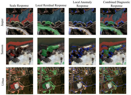
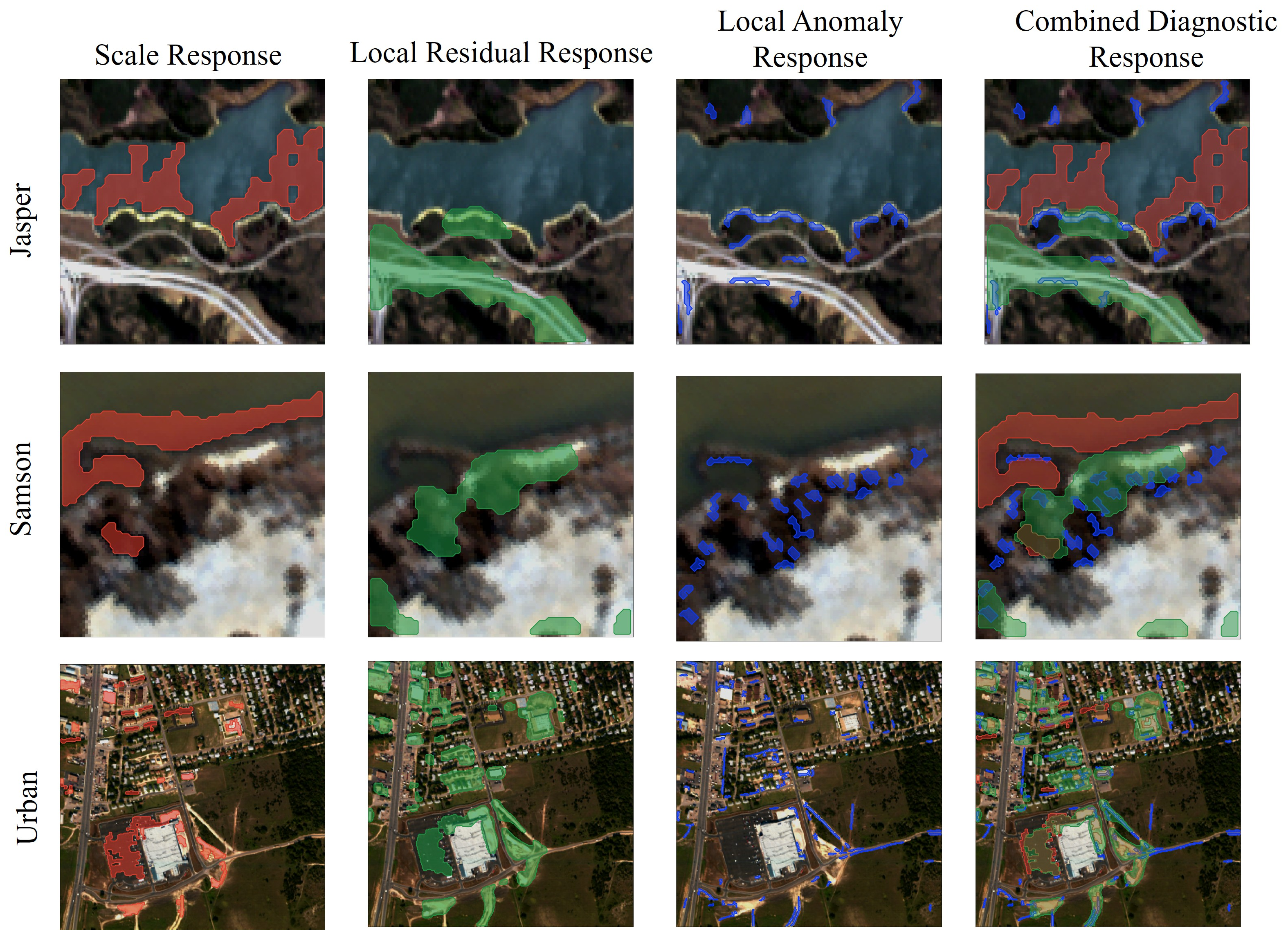
To further examine whether the proposed residual diagnostics capture meaningful mismatch patterns in real scenes, Figure 8 visualizes the spatial distributions of different diagnostic responses on the three benchmark datasets.

Figure 8. Spatial distributions of residual diagnostic responses on real datasets. Note: The red, green, and blue regions represent the scale response, local residual response, and local anomaly response, respectively. The combined diagnostic response overlays the three types of diagnostic regions.

The diagnostic responses exhibit different spatial patterns across the three datasets, suggesting that the residual descriptors capture complementary characteristics of the reconstruction mismatch. Their spatial differences also indicate that a single reconstruction-error measure is insufficient to summarize the residual structure, motivating the combined use of multiple diagnostic features in RDAC.

3.5.2. Abundance Correctability on Real-Scene Data

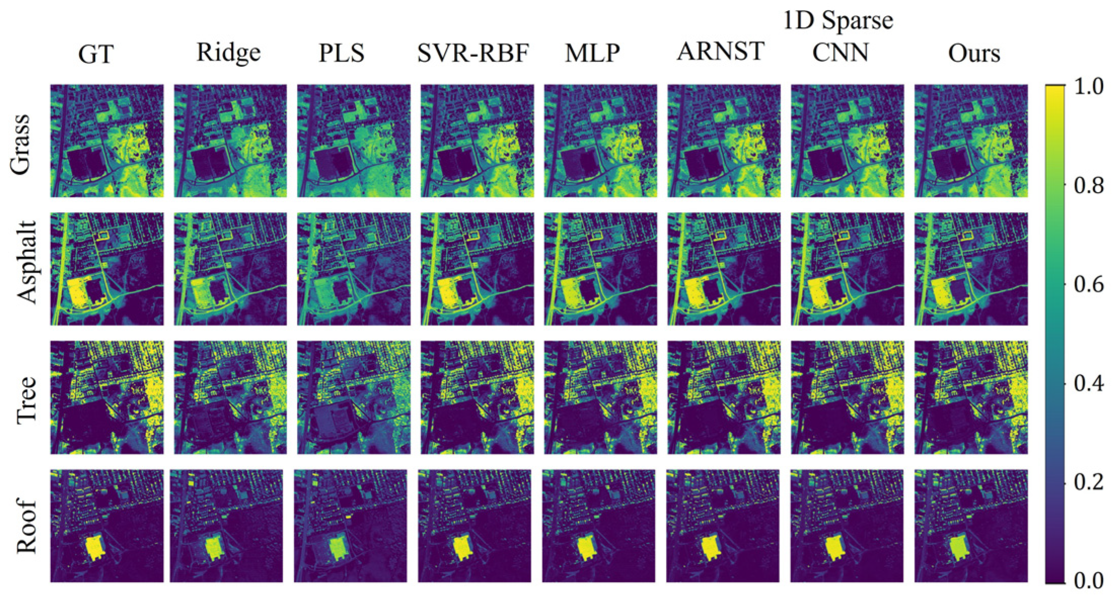
To clarify the labeling budget used in this comparison, the 1% reference-abundance setting corresponds to different absolute numbers of labeled training pixels across the three datasets because of their different image sizes. Specifically, 1% of the pixels amount to 100 labeled pixels for Jasper Ridge (100 × 100), 90 labeled pixels for Samson (95 × 95), and 942 labeled pixels for Urban (307 × 307), obtained by taking the floor of 1% of the total pixel count in each dataset. The remaining pixels were used for testing. Under the same 1% labeling budget, RDAC was compared with Ridge, PLS, SVR-RBF, MLP, ARNST, and 1D Sparse CNN. The direct supervised baselines learned the mapping from the observed spectra to the reference abundances using only the labeled training pixels, whereas RDAC used the blind-unmixing estimates together with residual descriptors constructed from the target image and used the labeled pixels only to learn the abundance correction. All methods used the same training–test split for each random seed, and the mean and standard deviation over five random repetitions were reported. No test reference abundances were used for model fitting or parameter selection.The comparison results are presented in Table 4.

Table 4. Test A-RMSE comparison under 1% labeled samples.

Dataset	Jasper	Samson	Urban
Blind A0	0.0509 ± 0.0001	0.0601 ± 0.0001	0.0889 ± 0.0001
Ridge	0.0460 ± 0.0028	0.0613 ± 0.0053	0.0851 ± 0.0006
PLS	0.0467 ± 0.0031	0.0605 ± 0.0028	0.0928 ± 0.0011
SVR-RBF	0.0240 ± 0.0015	0.0207 ± 0.0031	0.0203 ± 0.0003
MLP	0.0503 ± 0.0061	0.0402 ± 0.0129	0.0334 ± 0.0018
ARNST	0.0663 ± 0.0099	0.0617 ± 0.0158	0.0346 ± 0.0034
1D Sparse CNN	0.0525 ± 0.0022	0.0377 ± 0.0042	0.0349 ± 0.0015
Ours	0.0229 ± 0.0003	0.0175 ± 0.0007	0.0359 ± 0.0004

Note: The best results are highlighted in bold.

Table 4. Test A-RMSE comparison under 1% labeled samples.

Dataset	Jasper	Samson	Urban
Blind A0	0.0509 ± 0.0001	0.0601 ± 0.0001	0.0889 ± 0.0001
Ridge	0.0460 ± 0.0028	0.0613 ± 0.0053	0.0851 ± 0.0006
PLS	0.0467 ± 0.0031	0.0605 ± 0.0028	0.0928 ± 0.0011
SVR-RBF	0.0240 ± 0.0015	0.0207 ± 0.0031	0.0203 ± 0.0003
MLP	0.0503 ± 0.0061	0.0402 ± 0.0129	0.0334 ± 0.0018
ARNST	0.0663 ± 0.0099	0.0617 ± 0.0158	0.0346 ± 0.0034
1D Sparse CNN	0.0525 ± 0.0022	0.0377 ± 0.0042	0.0349 ± 0.0015
Ours	0.0229 ± 0.0003	0.0175 ± 0.0007	0.0359 ± 0.0004

Note: The best results are highlighted in bold.

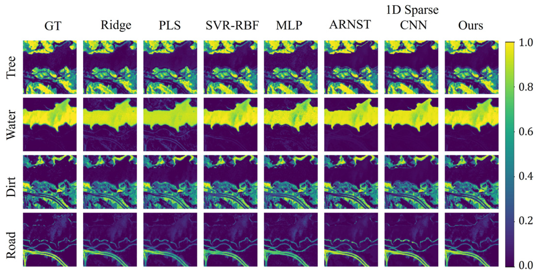
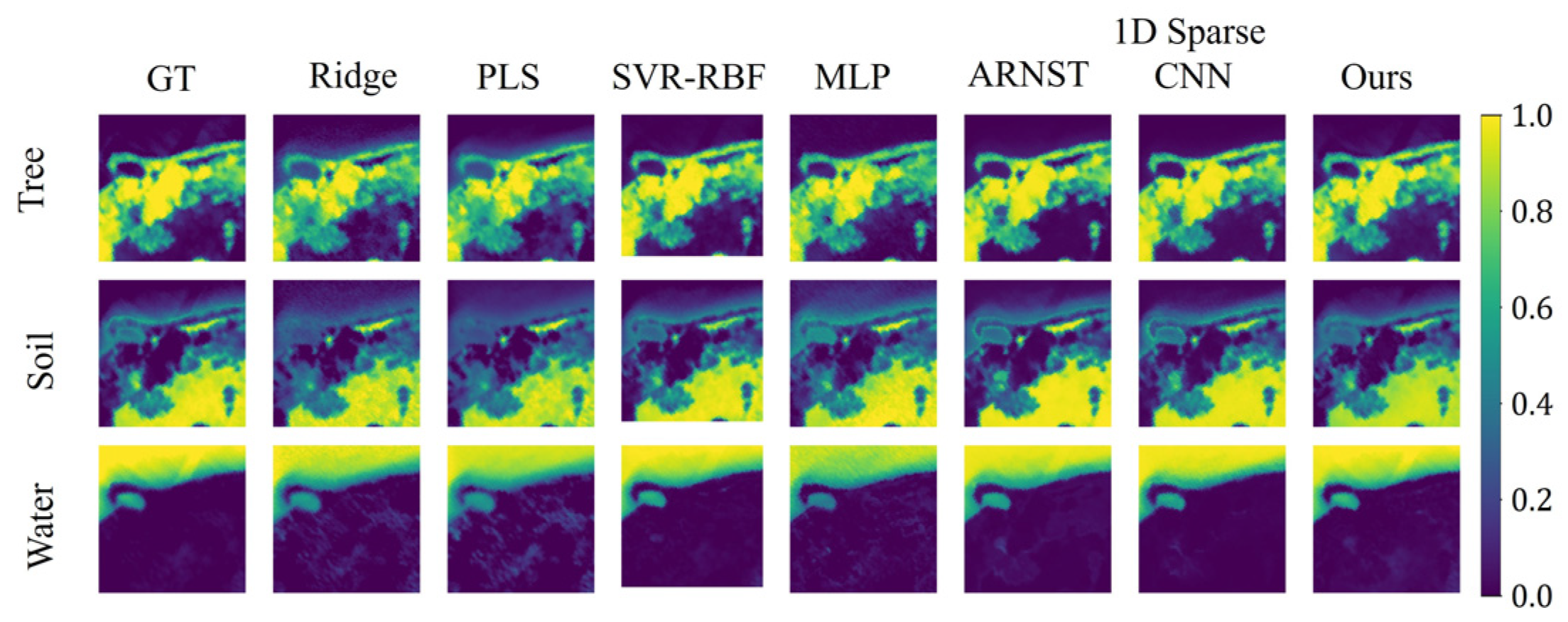
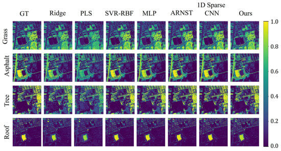
RDAC achieved the lowest mean A-RMSE on Jasper Ridge and Samson, whereas SVR-RBF achieved the lowest mean A-RMSE on Urban (0.0203 ± 0.0003). Relative to the initial abundance estimates A₀, RDAC reduced A-RMSE by 55.05%, 70.80%, and 59.63% on Jasper Ridge, Samson, and Urban, respectively.

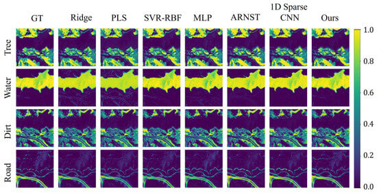
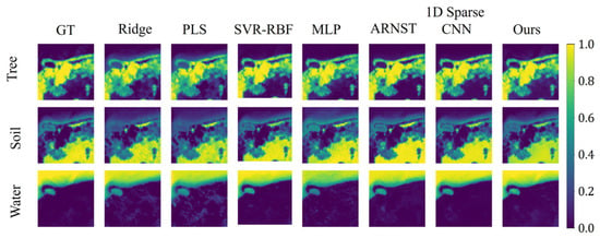
Figure 9, Figure 10 and Figure 11 show that the abundance maps are generally consistent with the quantitative results. RDAC more accurately recovered the spatial distributions of the major materials in Jasper Ridge and Samson, and also substantially improved the initial abundance estimates in Urban. However, its overall error in Urban remained higher than that of SVR-RBF.

Figure 9. Abundance comparison maps on the Jasper Ridge dataset.

Figure 10. Abundance comparison maps on the Samson dataset.

Figure 11. Abundance comparison maps on the Urban dataset.

3.5.3. Abundance Correction Behavior of RDAC

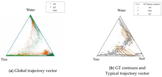
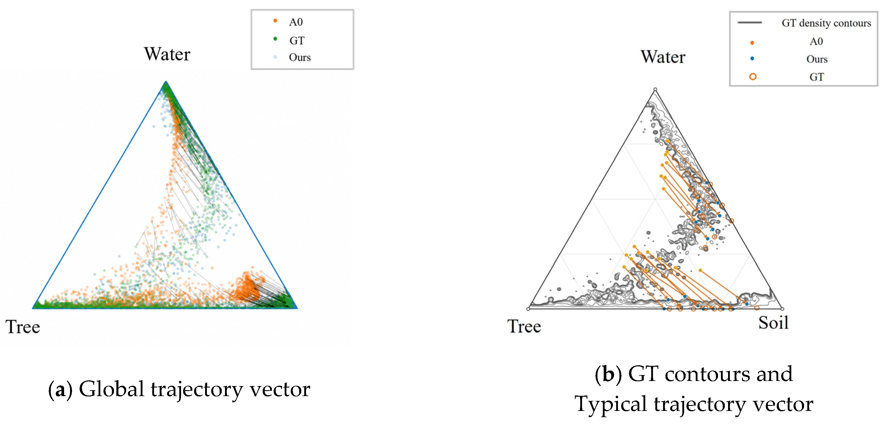
To examine how RDAC adjusts the initial abundance estimates, we visualized the abundance distributions before and after correction, together with the pixel-wise correction trajectories, in the abundance simplex of the Samson dataset.

Figure 12a shows that the ground-truth abundances (GT) are mainly distributed near the Water–Soil and Tree–Soil edges, indicating that the scene is dominated by pairwise mixtures involving these endmembers. The initial abundance estimates A₀ deviate noticeably from the GT distribution in the transition regions, whereas the RDAC-corrected abundances move closer to the main GT distribution, indicating that RDAC can reduce systematic biases in the initial abundance estimates. In Figure 12b, the correction trajectories mainly follow the Water–Soil and Tree–Soil directions and move closer to the corresponding GT locations, showing that RDAC adjusts the relative proportions among dominant endmembers while preserving the overall mixture structure. All trajectories remain within the physically feasible abundance simplex, further indicating that RDAC performs constrained corrections of the existing abundance estimates.

Figure 12. Global abundance distributions and correction trajectories in the Samson abundance simplex.

3.6. Experimental Validation

3.6.1. Comparison of Diagnostic Responses

A Raw Residual baseline was included to compare different representations of the reconstruction residual. All other settings were kept unchanged, including the initial abundance estimate A₀, the 1% training split, and the ridge-regression corrector. Abundance correction was performed using three feature configurations: (i) the raw reconstruction residual vector, (ii) the structured residual representation, and (iii) the complete RDAC feature set.

Table 5 shows that the Structured Residual representation yields lower errors than the Raw Residual baseline on all three datasets, while the complete RDAC feature set provides further improvement. These results indicate that, under limited supervision, organizing the high-dimensional residual into compact representations of its scale, spectral, spatial, and covariance structure is more effective for abundance correction than directly using the raw residual vector.

Table 5. Raw residual and structured residual ablation.

Dataset	Raw Residual	Structured Residual	Full
Jasper	0.0388 ± 0.0022	0.0294 ± 0.0016	0.0229 ± 0.0003
Samson	0.0296 ± 0.0013	0.0229 ± 0.0014	0.0175 ± 0.0007
Urban	0.0498 ± 0.0007	0.0481 ± 0.0006	0.0359 ± 0.0004

3.6.2. Component Ablation

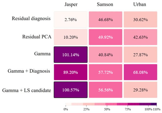
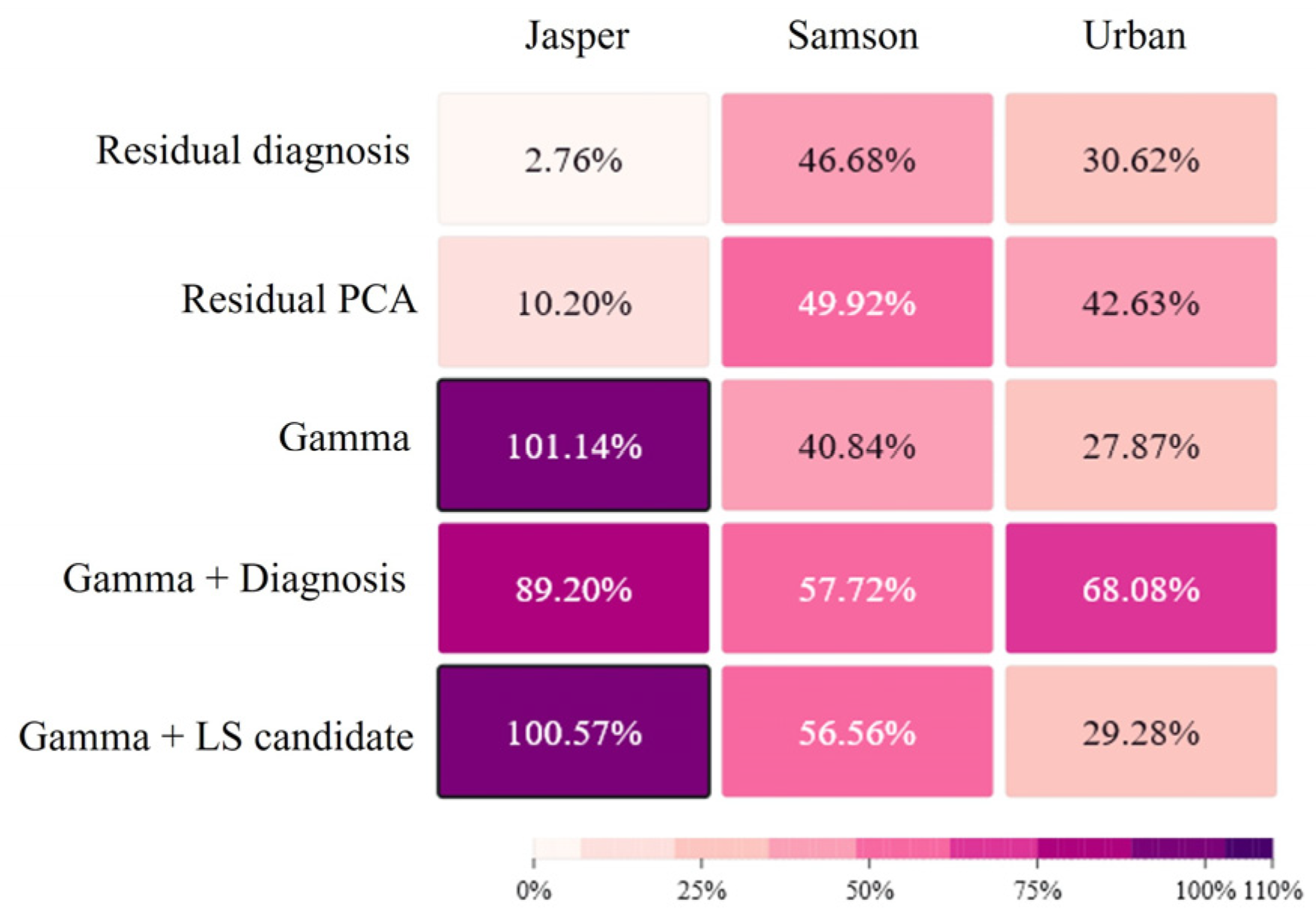
The ablation study was conducted under consistent experimental conditions. For each split, all variants used the same initial solution, training–test partition, and random seed. We compared the uncorrected A₀ with an A₀ calibration baseline and with variants that add the Gamma candidate, explicit residual diagnostics, Residual PCA, the fixed-endmember least-squares candidate, and the full feature combination. The A₀ calibration baseline uses only the initial abundance components a_0,i as input, excluding all candidate, diagnostic, and Residual PCA features, while sharing the same training pixels, ridge regularization, and abundance-increment target as full RDAC; its predicted increment is added to A₀ and followed by the same non-negative truncation and normalization. It thus differs from the uncorrected A₀, which involves no supervised calibration. Table 6 reports the results under the 1% labeled setting on the three datasets, while Figure 13 shows the corresponding A-RMSE changes relative to the A₀ calibration baseline.

Table 6. Component ablation results at the 1% training ratio.

Dataset	Jasper	Samson	Urban
A0	0.0509 ± 0.0001	0.0601 ± 0.0001	0.0889 ± 0.0001
A0 calibration	0.0303 ± 0.0011	0.0343 ± 0.0009	0.0585 ± 0.0006
A0 + Gamma	0.0228 ± 0.0003	0.0274 ± 0.0007	0.0522 ± 0.0003
A0 + Residual diagnosis	0.0300 ± 0.0011	0.0265 ± 0.0014	0.0516 ± 0.0006
A0 + Residual PCA	0.0295 ± 0.0016	0.0259 ± 0.0011	0.0489 ± 0.0006
A0 + LS candidate	0.0304 ± 0.0010	0.0309 ± 0.0009	0.0573 ± 0.0005
Full	0.0229 ± 0.0003	0.0175 ± 0.0007	0.0359 ± 0.0004

Figure 13. Relative improvements of component ablations over A₀ calibration.

The contributions of individual information sources varied across the three datasets. The Gamma candidate provided the largest individual improvement on Jasper Ridge, whereas Residual PCA contributed more strongly on Samson and Urban. The full feature combination achieved the lowest ablation error on Samson and Urban, although its performance on Jasper Ridge was comparable to that of the Gamma-only variant. These results suggest that the candidate abundances provide effective correction directions, while the residual descriptors characterize the current mismatch state and provide complementary information for determining how the initial abundance estimate should be adjusted. Their relative contributions are therefore dataset-dependent rather than dominated by a single component across all scenes.

3.6.3. Influence of the Correction Model

We compared Ridge regression, ordinary least squares (OLS), and SVR-RBF using the same Full RDAC feature representation, training–test splits, and random seeds. For each corrector, an A0-only variant was also tested to assess the effect of adding the full RDAC feature set beyond the initial abundance estimate. All other experimental settings were kept unchanged.

As shown in Table 7, the choice of correction model affects the final abundance accuracy. With the Full RDAC representation, SVR-RBF generally performs better than Ridge on Samson and Urban, while the difference on Jasper Ridge is smaller. The comparison with the A₀-only variants also shows that the added RDAC features do not contribute equally in all cases. Ridge and OLS benefit from the complete feature set on all three datasets, whereas SVR-RBF shows a stronger dependence on the dataset. The Full representation improves the results on Samson and Urban, but provides no advantage over A₀ alone on Jasper Ridge.

Table 7. Influence of the correction model on RDAC performance.

Corrector	Jasper Ridge	Samson	Urban
Ridge	0.0229 ± 0.0003	0.0175 ± 0.0007	0.0359 ± 0.0004
OLS	0.0233 ± 0.0001	0.0166 ± 0.0005	0.0359 ± 0.0004
SVR-RBF	0.0203 ± 0.0010	0.0132 ± 0.0014	0.0176 ± 0.0002

These results show that RDAC can be used with different correction models, although the effect of the complete feature set varies with the corrector and dataset. Ridge is kept as the default corrector because it offers a simple regularized setting for examining the RDAC features under limited supervision without adding unnecessary model complexity.

3.6.4. Model Complexity and Parameter Count

To assess the additional model complexity introduced by RDAC, we compared the number of trainable parameters in the RDAC correction stage with those of representative learning-based methods. Since RDAC operates as a post-correction module on an existing blind-unmixing solution, the parameter count of the correction stage is reported separately from that of the UNMamba backbone. For reference, the parameter counts of the 1D CNN and ARNST-style implementations are also included in the comparison, as reported in Table 8.

Table 8. Trainable parameter counts of RDAC and representative learning-based models.

Model or Stage	Jasper Ridge	Samson	Urban
RDAC corrector only	124	81	124
1D CNN implementation	172,100	171,971	172,100
ARNST-style implementation	42,250	42,185	42,250
UNMamba backbone	241,938	194,201	3,778,650
UNMamba + RDAC	242,062	194,282	3,778,774

Table 8. Trainable parameter counts of RDAC and representative learning-based models.

Model or Stage	Jasper Ridge	Samson	Urban
RDAC corrector only	124	81	124
1D CNN implementation	172,100	171,971	172,100
ARNST-style implementation	42,250	42,185	42,250
UNMamba backbone	241,938	194,201	3,778,650
UNMamba + RDAC	242,062	194,282	3,778,774

The RDAC correction stage introduces only 124, 81, and 124 trainable parameters on Jasper Ridge, Samson, and Urban, respectively. These values are much smaller than those of the 1D CNN and ARNST-style implementations. When RDAC is combined with UNMamba, the additional trainable parameters account for only a very small fraction of the backbone size. Therefore, the improvement obtained by RDAC is achieved with limited additional trainable complexity, while the main computational cost remains in the initial blind-unmixing backbone and the construction of the correction features.

3.7. Experimental Robustness Analysis

3.7.1. Label Efficiency

To examine the effect of the amount of reference abundance supervision, the labeled-sample ratios were set to 0.05%, 0.1%, 0.2%, 0.5%, 1%, 5%, 10%, 30%, and 50%. For each ratio, the corresponding proportion of labeled pixels was independently sampled from the target scene as the training set, with the remaining pixels used for testing. The same set of five random seeds was used at each ratio to ensure consistent and reproducible evaluation, while the training samples were independently generated for each ratio.The results are shown in Figure 14.

Figure 14. Effect of the labeled-sample ratio on abundance correction performance.

Figure 14. Effect of the labeled-sample ratio on abundance correction performance.

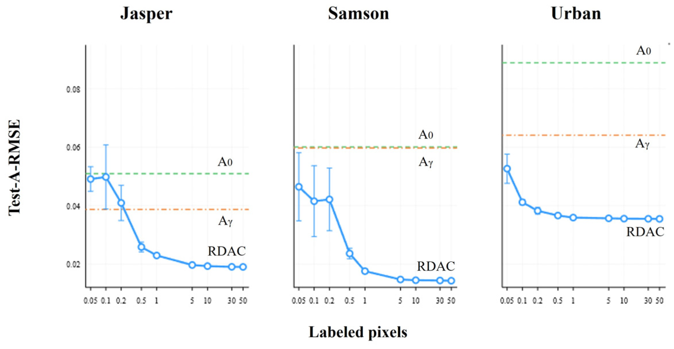
At a labeled-sample ratio of 0.5%, Jasper Ridge, Samson, and Urban contained 50, 45, and 471 training pixels, respectively, yielding test A-RMSE values of 0.0258, 0.0236, and 0.0366. When the ratio increased to 1%, the corresponding A-RMSE values decreased to 0.0229, 0.0175, and 0.0359, respectively. Beyond a labeled-sample ratio of approximately 5%, the performance curves for all three datasets gradually approached a plateau.

3.7.2. Spatial Generalization

Random pixel-wise splitting may place training and test samples in close spatial proximity. To mitigate this effect, we further constructed the training and test sets using non-overlapping spatial regions. Because a 1% spatial-block split provided insufficient training coverage for some methods, this experiment used a 5% labeling ratio for all methods and compared the results with those obtained under random pixel-wise splitting at the same 5% labeling ratio.The results are reported in Table 9.

Table 9. Random-pixel and spatial-block split comparison.

Dataset	Division Method	A0	SVR-RBF	MLP	RDAC 5%
Jasper	Random	0.0510 ± 0.0001	0.0146 ± 0.0003	0.0325 ± 0.0028	0.0196 ± 0.0002
	Block	0.0509 ± 0.0004	0.0321 ± 0.0095	0.0568 ± 0.0163	0.0246 ± 0.0035
Samson	Random	0.0600 ± 0.0001	0.0127 ± 0.0003	0.0242 ± 0.0033	0.0147 ± 0.0001
	Block	0.0608 ± 0.0005	0.0333 ± 0.0117	0.0509 ± 0.0139	0.0236 ± 0.0047
Urban	Random	0.0889 ± 0.0001	0.0157 ± 0.0001	0.0193 ± 0.0039	0.0356 ± 0.0001
	Block	0.0889 ± 0.0003	0.0209 ± 0.0018	0.0234 ± 0.0057	0.0390 ± 0.0010

Table 9. Random-pixel and spatial-block split comparison.

Dataset	Division Method	A0	SVR-RBF	MLP	RDAC 5%
Jasper	Random	0.0510 ± 0.0001	0.0146 ± 0.0003	0.0325 ± 0.0028	0.0196 ± 0.0002
	Block	0.0509 ± 0.0004	0.0321 ± 0.0095	0.0568 ± 0.0163	0.0246 ± 0.0035
Samson	Random	0.0600 ± 0.0001	0.0127 ± 0.0003	0.0242 ± 0.0033	0.0147 ± 0.0001
	Block	0.0608 ± 0.0005	0.0333 ± 0.0117	0.0509 ± 0.0139	0.0236 ± 0.0047
Urban	Random	0.0889 ± 0.0001	0.0157 ± 0.0001	0.0193 ± 0.0039	0.0356 ± 0.0001
	Block	0.0889 ± 0.0003	0.0209 ± 0.0018	0.0234 ± 0.0057	0.0390 ± 0.0010

Under the spatial-block split, RDAC still achieved lower A-RMSE than the compared supervised methods on Jasper Ridge and Samson, whereas SVR-RBF retained a clear advantage on Urban. Compared with random pixel-wise splitting, all methods exhibited varying degrees of performance change under the spatial-block setting, indicating that the spatial coverage and representativeness of reference samples can affect generalization under limited supervision.

3.7.3. Statistical Stability

To complement the comparison of mean performance, RDAC and SVR-RBF were further evaluated using paired statistical tests over the same 30 random splits. A two-sided paired t-test was performed for each dataset, and Holm correction was applied to the three dataset-wise comparisons. The paired mean difference, 95% confidence interval, Cohen’s d_z, and adjusted p-value are reported in Table 10.

Table 10. Statistical stability analysis across 30 random seeds.

Dataset	Mean Difference (SVR − RDAC)	95% CI	Cohen’s dz	Holm-Adjusted Paired t-Test
Jasper Ridge	0.001625	[0.000638, 0.002612]	0.615	0.00648
Samson	0.002752	[0.001961, 0.003542]	1.300	3.91 × 10−7
Urban	−0.015851	[−0.016050, −0.015653]	−29.822	3.06 × 10−43

RDAC achieved lower mean A-RMSE than SVR-RBF on Jasper Ridge and Samson, with Holm-adjusted p-values of 0.00648 and 3.91 × 10⁻⁷, respectively. On Urban, SVR-RBF performed better, with an adjusted p-value of 3.06 × 10⁻⁴³. The statistical results are therefore consistent with the differences observed in the mean A-RMSE across the three datasets.

3.7.4. Parameter Sensitivity

We further analyzed the sensitivity of RDAC to three key parameters: the Residual PCA dimension q, the ridge-regression coefficient λ, and the Gamma exponent γ. The corresponding results are presented in Figure 15 and Figure 16.

Figure 15. Sensitivity to residual PCA dimension q and ridge coefficient λ.

Figure 15. Sensitivity to residual PCA dimension q and ridge coefficient λ.

Figure 16. Sensitivity to the Gamma exponent γ.

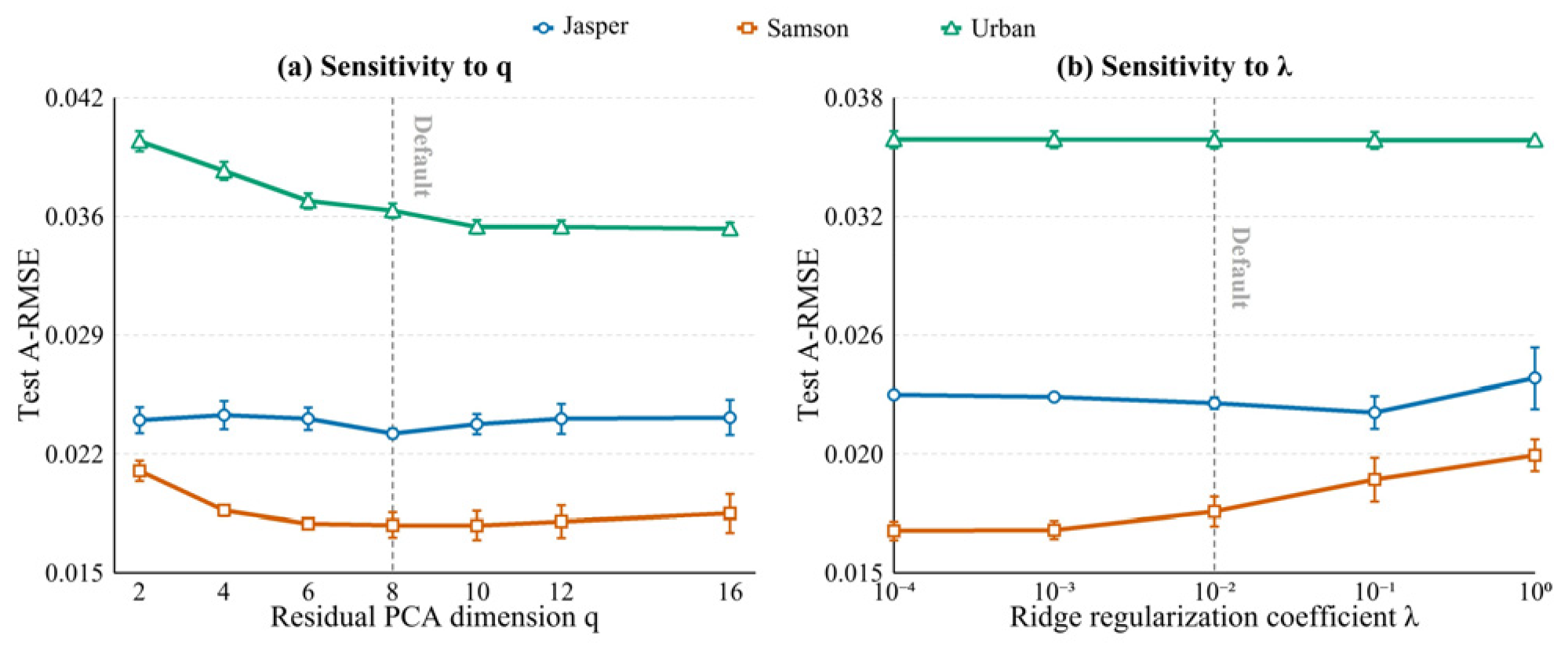
Figure 16. Sensitivity to the Gamma exponent γ.

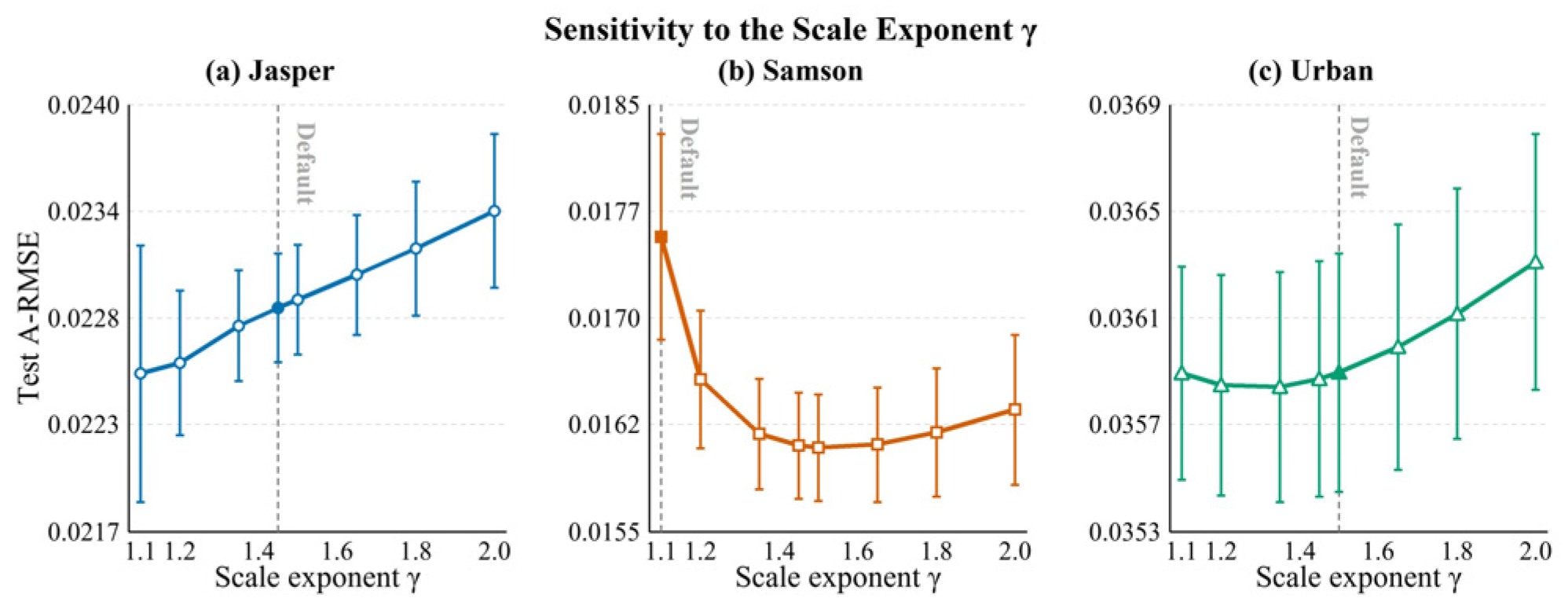
When q reached approximately 8, the performance on all three datasets became relatively stable. Performance changed only slightly over a broad range of λ values, whereas the performance-sensitive range of γ differed more noticeably across datasets, although the values selected from the training reference abundances remained within competitive regions. These results indicate that RDAC is relatively robust to the Residual PCA dimension and ridge-regression regularization, while the Gamma-based redistribution is more sensitive to dataset-specific patterns of initial abundance bias.

3.7.5. Effect of Residual PCA Construction

The default RDAC implementation estimates the Residual PCA basis from the reconstruction residuals of all pixels in the target scene. To evaluate the contribution of full-scene information, two additional settings were considered: Training-only PCA, where the PCA basis is estimated using only the labeled training pixels, and No PCA, where the Residual PCA features are removed. All other components and experimental settings were kept unchanged.

As shown in Table 11, Training-only PCA gives results very close to those of Full-scene PCA. Relative to the Full-scene setting, the mean A-RMSE changes by +0.98% on Jasper Ridge, −0.48% on Samson, and +0.02% on Urban. Removing the Residual PCA features has a larger effect. Compared with the No-PCA setting, Full-scene PCA reduces the mean A-RMSE by 2.85%, 19.82%, and 15.99% on Jasper Ridge, Samson, and Urban, respectively.

Table 11. Comparison of different Residual PCA construction settings.

PCA Setting	Jasper Ridge	Samson	Urban
Full-scene PCA	0.0229 ± 0.0003	0.0175 ± 0.0007	0.0359 ± 0.0004
Training-only PCA	0.0231 ± 0.0003	0.0175 ± 0.0006	0.0359 ± 0.0004
No PCA	0.0236 ± 0.0004	0.0219 ± 0.0007	0.0427 ± 0.0003

These results help distinguish the effect of the Residual PCA representation from that of using full-scene samples to estimate the PCA basis. Residual PCA contributes useful correction information, especially on Samson and Urban, while fitting the basis on the full target scene brings only a small additional benefit over using the labeled training pixels under the 1% supervision setting. The main contribution of this component therefore comes from the residual subspace representation itself rather than from full-scene PCA fitting.

4. Discussion

4.1. Consistency of Reconstructed Spectra After Correction

We compared abundance accuracy with two spectral reconstruction measures before and after RDAC. In addition to reconstruction RMSE, the mean spectral angle between the observed and reconstructed spectra was calculated to describe changes in spectral shape.

As shown in Table 12, RDAC improves abundance accuracy on all three datasets, while the reconstruction measures do not follow the same trend. The reconstruction RMSE changes little on Jasper Ridge but increases on Samson and Urban, and the mean spectral angle also becomes larger after correction.

Table 12. Reconstruction consistency before and after RDAC.

Dataset	Jasper Ridge	Samson	Urban
A-RMSE Initial	0.0509	0.0601	0.0889
A-RMSE RDAC	0.0227	0.0178	0.0359
A-RMSE Reduction	55.51%	70.39%	59.57%
Recon. RMSE Initial	0.0796	0.0852	0.0776
Recon. RMSE RDAC	0.0797	0.0882	0.0787
Recon. Change	0.08%	3.47%	1.38%
Mean Spectral Angle Initial (°)	≈3.576	≈2.012	≈2.778
Mean Spectral Angle RDAC (°)	≈4.472	≈3.274	≈4.762

This difference is expected when the abundances are corrected while the estimated endmembers remain fixed. Abundances that are closer to the reference values do not necessarily give the smallest reconstruction error under the same endmember set. For this reason, reconstruction RMSE and spectral angle are reported separately from abundance accuracy and are used only to describe the change in spectral reconstruction after correction.

4.2. Cross-Backbone Evaluation

To assess whether RDAC depends on the primary UNMamba backbone, we applied the same correction procedure to abundance and endmember estimates obtained from NMF without changing the framework. Abundance accuracy was then evaluated on the same three datasets.

As shown in Table 13, RDAC substantially reduced A-RMSE on all three datasets when applied to the NMF-based initial solution. This suggests that the correction strategy can also be applied beyond the primary UNMamba backbone. The NMF experiment also provides an example in which the initial abundance estimates contain much larger errors than those obtained with UNMamba. RDAC still substantially reduces the abundance error in this case, indicating that the correction does not require a highly accurate initial abundance estimate. Since only UNMamba and NMF were evaluated, further experiments with other blind-unmixing methods are still needed to assess the broader applicability of RDAC.

Table 13. RDAC portability with an NMF blind-unmixing backbone.

Dataset	NMF A0 A-RMSE	NMF + RDAC Full A-RMSE	Gain
Jasper	0.1763 ± 0.0001	0.0345 ± 0.0020	80.45%
Samson	0.2030 ± 0.0001	0.0218 ± 0.0015	89.25%
Urban	0.2003 ± 0.0001	0.0448 ± 0.0005	77.61%

To better understand the large performance gains obtained with the NMF initialization, we carried out an additional ablation study using NMF as the blind-unmixing backbone. Under the same correction setting, the experiment examines the contribution of limited-reference calibration and of each feature group separately.The results are presented in Table 14.

Table 14. Component ablation with an NMF blind-unmixing backbone.

Configuration	Jasper Ridge	Samson	Urban
NMF A0	0.1763	0.2030	0.2003
A 0 calibration	0.0571	0.0548	0.0825
A 0 + Gamma	0.0467	0.0383	0.0680
A 0 + LS	0.0448	0.0448	0.0690
A 0 + LS difference	0.0449	0.0448	0.0690
A 0 + Diagnosis	0.0521	0.0455	0.0711
A 0 + PCA	0.0361	0.0385	0.0685
Full RDAC	0.0345	0.0218	0.0448

Table 14. Component ablation with an NMF blind-unmixing backbone.

Configuration	Jasper Ridge	Samson	Urban
NMF A0	0.1763	0.2030	0.2003
A 0 calibration	0.0571	0.0548	0.0825
A 0 + Gamma	0.0467	0.0383	0.0680
A 0 + LS	0.0448	0.0448	0.0690
A 0 + LS difference	0.0449	0.0448	0.0690
A 0 + Diagnosis	0.0521	0.0455	0.0711
A 0 + PCA	0.0361	0.0385	0.0685
Full RDAC	0.0345	0.0218	0.0448

The results show that supervised calibration of the initial abundance already accounts for a substantial part of the improvement over the original NMF solution, highlighting the role of the limited reference abundances. The candidate and residual-related feature groups provide further gains, although their contributions differ across datasets. The full RDAC representation gives the best overall performance on all three datasets, showing that the improvement comes from the combined use of different feature groups rather than from any single component.

The larger initial NMF error does not lead to a consistently larger relative improvement across datasets. The correction gain therefore depends not only on the initial error magnitude, but also on the structure of the initial solution and the usefulness of the available correction information.

4.3. Urban Result Analysis

We conducted several diagnostic experiments to examine the weaker performance of the Ridge-based RDAC on Urban. The analysis focused on the quality of the initial abundance estimate, the spatial distribution of the reference samples, and whether grouping pixels with different feature patterns could improve the correction. The default Ridge-based RDAC result was used as the reference. The results are summarized in Table 15.

Table 15. Diagnostic analysis of factors affecting RDAC performance on the Urban dataset.

Analysis	Setting	Corrector	Urban A-RMSE
Initial-abundance quality	Original initial abundance	Ridge	0.0359
	Perturbed initial abundance		0.0395
Reference sample distribution	Random reference sampling	Ridge	0.0359
	Spatially concentrated sampling		0.0450
Grouped correction	Global Ridge	Ridge	0.0359
	Feature-based two-group Ridge		0.0297
	Random two-group Ridge		0.0364

The Urban results are affected by the quality of the initial abundance estimate, the spatial distribution of the reference samples, and the choice of correction model. As shown in Table 7 of Section 3.6.3, SVR-RBF gives a lower A-RMSE than the global linear models on Urban, suggesting that a more flexible correction model may be needed for this dataset.

The grouped-correction experiment gives a consistent result. Grouping pixels according to their diagnostic features improves the correction, whereas random grouping does not. This suggests that the improvement is related to differences in the correction relationships among pixels rather than simply to the use of multiple regressors.

These results suggest that a single global Ridge model may not fully capture the correction relationship in the Urban dataset.

4.4. Method Limitations and Future Work

The current RDAC formulation is mainly constrained by three factors. Because the correction is performed with the estimated endmembers E₀ held fixed, large endmember errors cannot always be compensated for by adjusting the abundances alone. The method also depends on a small set of reference abundances, so noisy labels or poor spatial coverage may reduce the reliability of the learned correction. In addition, the Residual PCA basis and several residual statistics are derived from the full target scene, which means that the present implementation remains transductive and scene-specific. These limitations point to several possible extensions, including joint refinement of endmembers and abundances, more informative sample selection, and uncertainty-aware supervision. Extending the method to noisy reference labels and to inductive correction across different scenes and sensors is another direction worth exploring.

5. Conclusions

In blind hyperspectral unmixing, reconstruction fidelity alone does not fully reflect the reliability of the estimated abundances. RDAC uses structured reconstruction residuals to refine existing abundance estimates instead of relearning the complete mapping from spectra to abundances. Experiments on Jasper Ridge, Samson, and Urban show that structured residual representations provide more useful correction information than raw residuals, and that abundance accuracy can be improved using only 1% reference samples. The NMF experiment further shows that the same correction procedure can be applied to an alternative blind-unmixing backbone.

Because RDAC corrects the abundances while keeping the estimated endmembers fixed, its performance still depends on the quality of the initial unmixing result, and large endmember errors cannot always be compensated for by abundance correction alone. The spatial distribution of the limited reference samples also affects the correction. Future work will focus on joint refinement of endmembers and abundances and on more robust correction strategies when reference samples are sparse or unevenly distributed.

References

- Rasti, B.; Zouaoui, A.; Mairal, J.; Chanussot, J. Image processing and machine learning for hyperspectral unmixing: An overview and the HySUPP Python package. IEEE Trans. Geosci. Remote Sens. 2024, 62, 5517631. [Google Scholar] [CrossRef] [Scilit]
- Bioucas-Dias, J.M.; Plaza, A.; Dobigeon, N.; Parente, M.; Du, Q.; Gader, P.; Chanussot, J. Hyperspectral unmixing overview: Geometrical, statistical, and sparse regression-based approaches. IEEE J. Sel. Top. Appl. Earth Obs. Remote Sens. 2012, 5, 354–379. [Google Scholar] [CrossRef] [Scilit]
- Huo, Y.; Wang, S.; Wang, C.; Zhang, M.; Wang, H. Dual-stream background modeling network with anomaly suppression for hyperspectral anomaly detection. Int. J. Appl. Earth Obs. Geoinf. 2026, 148, 105233. [Google Scholar] [CrossRef] [Scilit]
- Luo, X.; Xu, W.; Jiang, Y. Group-Aware Spectral Perturbation Consistency Network for Cross-Domain Few-Shot Hyperspectral Image Classification. Remote Sens. 2026, 18, 3423. [Google Scholar] [CrossRef] [Scilit]
- Ren, L.; Han, Z.; Gao, L.; Zhang, T.; Wu, R.; Zhang, H. Advances in hyperspectral image unmixing: From algorithmic frameworks to practical applications. Inf. Geogr. 2026, 2, 100035. [Google Scholar] [CrossRef] [Scilit]
- Nascimento, J.M.P.; Dias, J.M.B. Vertex component analysis: A fast algorithm to unmix hyperspectral data. IEEE Trans. Geosci. Remote Sens. 2005, 43, 898–910. [Google Scholar] [CrossRef] [Scilit]
- Chan, T.-H.; Chi, C.-Y.; Huang, Y.-M.; Ma, W.-K. A convex analysis-based minimum-volume enclosing simplex algorithm for hyperspectral unmixing. IEEE Trans. Signal Process. 2009, 57, 4418–4432. [Google Scholar] [CrossRef] [Scilit]
- Li, J.; Agathos, A.; Zaharie, D.; Bioucas-Dias, J.M.; Plaza, A.; Li, X. Minimum volume simplex analysis: A fast algorithm for linear hyperspectral unmixing. IEEE Trans. Geosci. Remote Sens. 2015, 53, 5067–5082. [Google Scholar] [CrossRef] [Scilit]
- Miao, L.; Qi, H. Endmember extraction from highly mixed data using minimum volume constrained nonnegative matrix factorization. IEEE Trans. Geosci. Remote Sens. 2007, 45, 765–777. [Google Scholar] [CrossRef] [Scilit]
- Qian, Y.; Jia, S.; Zhou, J.; Robles-Kelly, A. Hyperspectral unmixing via L1/2 sparsity-constrained nonnegative matrix factorization. IEEE Trans. Geosci. Remote Sens. 2011, 49, 4282–4297. [Google Scholar] [CrossRef] [Scilit]
- Lu, X.; Wu, H.; Yuan, Y.; Yan, P.; Li, X. Manifold regularized sparse NMF for hyperspectral unmixing. IEEE Trans. Geosci. Remote Sens. 2013, 51, 2815–2826. [Google Scholar] [CrossRef] [Scilit]
- Eches, O.; Dobigeon, N.; Mailhes, C.; Tourneret, J.-Y. Bayesian estimation of linear mixtures using the normal compositional model. Application to hyperspectral imagery. IEEE Trans. Image Process. 2010, 19, 1403–1413. [Google Scholar] [CrossRef] [Scilit] [PubMed]
- Eches, O.; Dobigeon, N.; Tourneret, J.-Y. Enhancing hyperspectral image unmixing with spatial correlations. IEEE Trans. Geosci. Remote Sens. 2011, 49, 4239–4247. [Google Scholar] [CrossRef] [Scilit]
- Dobigeon, N.; Moussaoui, S.; Coulon, M.; Tourneret, J.-Y.; Hero, A.O. Joint Bayesian endmember extraction and linear unmixing for hyperspectral imagery. IEEE Trans. Signal Process. 2009, 57, 4355–4368. [Google Scholar] [CrossRef] [Scilit]
- Cruz-Guerrero, I.A.; Mejía-Rodríguez, A.R.; Ortega, S.; Fabelo, H.; Callico, G.M.; Jo, J.A.; Campos-Delgado, D.U. Multi and hyperspectral image unmixing with spatial coherence by extended blind end-member and abundance extraction. J. Frankl. Inst. 2023, 360, 11165–11196. [Google Scholar] [CrossRef] [Scilit]
- Zou, J.; Qu, H.; Zhang, P. Conventional to deep learning methods for hyperspectral unmixing: A review. Remote Sens. 2025, 17, 2968. [Google Scholar] [CrossRef] [Scilit]
- Zhang, M.; Yang, M.; Xie, H.; Yue, P.; Zhang, W.; Jiao, Q.; Xu, L.; Tan, X. A global spatial–spectral feature fused autoencoder for nonlinear hyperspectral unmixing. Remote Sens. 2024, 16, 3149. [Google Scholar] [CrossRef] [Scilit]
- Palsson, B.; Sigurdsson, J.; Sveinsson, J.R.; Ulfarsson, M.O. Hyperspectral unmixing using a neural network autoencoder. IEEE Access 2018, 6, 25646–25656. [Google Scholar] [CrossRef] [Scilit]
- Zhang, X.; Sun, Y.; Zhang, J.; Wu, P.; Jiao, L. Hyperspectral unmixing via deep convolutional neural networks. IEEE Geosci. Remote Sens. Lett. 2018, 15, 1755–1759. [Google Scholar] [CrossRef] [Scilit]
- Ghosh, P.; Roy, S.K.; Koirala, B.; Rasti, B.; Scheunders, P. Hyperspectral unmixing using transformer network. IEEE Trans. Geosci. Remote Sens. 2022, 60, 5535116. [Google Scholar] [CrossRef] [Scilit]
- Wang, P.; Liu, R.; Zhang, L. MAT-Net: Multiscale aggregation transformer network for hyperspectral unmixing. IEEE Trans. Geosci. Remote Sens. 2024, 62, 5538115. [Google Scholar] [CrossRef] [Scilit]
- Zhang, M.; Xie, H.; Yang, M.; Jiao, Q.; Xu, L.; Tan, X. Mamba-enhanced spatial–spectral feature learning for hyperspectral unmixing. IEEE J. Sel. Top. Appl. Earth Obs. Remote Sens. 2025, 18, 22798–22815. [Google Scholar] [CrossRef] [Scilit]
- Chen, D.; Zhang, J.; Li, J. UNMamba: Cascaded spatial–spectral Mamba for blind hyperspectral unmixing. IEEE Geosci. Remote Sens. Lett. 2025, 22, 5502405. [Google Scholar] [CrossRef] [Scilit]
- Liu, H.; Zhang, Y.; Li, Y.; Wang, Y.; Chen, X. A two-stage decoupling framework for blind hyperspectral unmixing: Separately refining endmembers and abundances. Remote Sens. 2026, 18, 2080. [Google Scholar] [CrossRef] [Scilit]
- Rasti, B.; Koirala, B.; Scheunders, P.; Ghamisi, P. How hyperspectral image unmixing and denoising can boost each other. Remote Sens. 2020, 12, 1728. [Google Scholar] [CrossRef] [Scilit]
- Somers, B.; Asner, G.P.; Tits, L.; Coppin, P. Endmember variability in spectral mixture analysis: A review. Remote Sens. Environ. 2011, 115, 1603–1616. [Google Scholar] [CrossRef] [Scilit]
- Zhang, C.; Ma, L.; Chen, J.; Rao, Y.; Zhou, Y.; Chen, X. Assessing the impact of endmember variability on linear spectral mixture analysis (LSMA): A theoretical and simulation analysis. Remote Sens. Environ. 2019, 235, 111471. [Google Scholar] [CrossRef] [Scilit]
- Thouvenin, P.-A.; Dobigeon, N.; Tourneret, J.-Y. Hyperspectral unmixing with spectral variability using a perturbed linear mixing model. IEEE Trans. Signal Process. 2016, 64, 525–538. [Google Scholar] [CrossRef] [Scilit]
- Drumetz, L.; Veganzones, M.-A.; Henrot, S.; Phlypo, R.; Chanussot, J.; Jutten, C. Blind hyperspectral unmixing using an extended linear mixing model to address spectral variability. IEEE Trans. Image Process. 2016, 25, 3890–3905. [Google Scholar] [CrossRef] [Scilit] [PubMed]
- Hong, D.; Yokoya, N.; Chanussot, J.; Zhu, X.X. An augmented linear mixing model to address spectral variability for hyperspectral unmixing. IEEE Trans. Image Process. 2019, 28, 1923–1938. [Google Scholar] [CrossRef] [Scilit] [PubMed]
- Cheng, Y.; Zhao, L.; Chen, S.; Li, X. Hyperspectral unmixing network accounting for spectral variability based on a modified scaled and a perturbed linear mixing model. Remote Sens. 2023, 15, 3890. [Google Scholar] [CrossRef] [Scilit]
- Su, L.; Liu, J.; Yuan, Y.; Chen, Q. A multi-attention autoencoder for hyperspectral unmixing based on the extended linear mixing model. Remote Sens. 2023, 15, 2898. [Google Scholar] [CrossRef] [Scilit]
- Halimi, A.; Altmann, Y.; Dobigeon, N.; Tourneret, J.-Y. Nonlinear unmixing of hyperspectral images using a generalized bilinear model. IEEE Trans. Geosci. Remote Sens. 2011, 49, 4153–4162. [Google Scholar] [CrossRef] [Scilit]
- Altmann, Y.; Halimi, A.; Dobigeon, N.; Tourneret, J.-Y. Supervised nonlinear spectral unmixing using a postnonlinear mixing model for hyperspectral imagery. IEEE Trans. Image Process. 2012, 21, 3017–3025. [Google Scholar] [CrossRef] [Scilit] [PubMed]
- Altmann, Y.; Dobigeon, N.; McLaughlin, S.; Tourneret, J.-Y. Residual component analysis of hyperspectral images—Application to joint nonlinear unmixing and nonlinearity detection. IEEE Trans. Image Process. 2014, 23, 2148–2158. [Google Scholar] [CrossRef] [Scilit] [PubMed]
- Xiang, S.; Li, X.; Chen, S. An endmember-oriented transformer network for bundle-based hyperspectral unmixing. IEEE Trans. Geosci. Remote Sens. 2025, 63, 5503315. [Google Scholar] [CrossRef] [Scilit]
- Zhang, S.; Zhou, X.; Li, K.; Fu, J.; Chen, X.; Zhou, J.; Lai, P.; Li, F.; Deng, C.; Wang, S. Residual-guided dual-spatial weighted sparse NMF for robust blind spectral unmixing. Infrared Phys. Technol. 2026, 159, 106872. [Google Scholar] [CrossRef] [Scilit]
- Yi, X.; Jin, Z.; Liu, Y.; Zhang, H. Interpretable deep network harnessing spectral variability similarity for accurate hyperspectral unmixing. Knowl.-Based Syst. 2026, 331, 114756. [Google Scholar] [CrossRef] [Scilit]
- Zeng, Y.; Ritz, C.; Zhao, J.; Lan, J. Attention-based residual network with scattering transform features for hyperspectral unmixing with limited training samples. Remote Sens. 2020, 12, 400. [Google Scholar] [CrossRef] [Scilit]
- Huang, J.; Zhang, P. Beyond pixel-wise unmixing: Spatial–spectral attention fully convolutional networks for abundance estimation. Remote Sens. 2023, 15, 5694. [Google Scholar] [CrossRef] [Scilit]
- Wan, L.; Chen, T.; Plaza, A.; Cai, H. Hyperspectral unmixing based on spectral and sparse deep convolutional neural networks. IEEE J. Sel. Top. Appl. Earth Obs. Remote Sens. 2021, 14, 11669–11682. [Google Scholar] [CrossRef] [Scilit]
- Xu, X.; Shi, Z.; Pan, B. A supervised abundance estimation method for hyperspectral unmixing. Remote Sens. Lett. 2018, 9, 383–392. [Google Scholar] [CrossRef] [Scilit]
- Das, S.; Routray, A.; Deb, A.K. Fast semi-supervised unmixing of hyperspectral image by mutual coherence reduction and recursive PCA. Remote Sens. 2018, 10, 1106. [Google Scholar] [CrossRef] [Scilit]
- Tan, X.; Yu, Q.; Wang, Z.; Zhu, J. Semi-supervised unmixing of hyperspectral data via spectral–spatial factorization. IEEE Sens. J. 2021, 21, 25963–25972. [Google Scholar] [CrossRef] [Scilit]
- Chen, B.; Lou, Y.; Bertozzi, A.L.; Chanussot, J. Graph-based active learning for nearly blind hyperspectral unmixing. IEEE Trans. Geosci. Remote Sens. 2023, 61, 5523716. [Google Scholar] [CrossRef] [Scilit]
Disclaimer/Publisher’s Note: The statements, opinions and data contained in all publications are solely those of the individual author(s) and contributor(s) and not of MDPI and/or the editor(s). MDPI and/or the editor(s) disclaim responsibility for any injury to people or property resulting from any ideas, methods, instructions or products referred to in the content. |
© 2026 by the authors. Licensee MDPI, Basel, Switzerland. This article is an open access article distributed under the terms and conditions of the Creative Commons Attribution (CC BY) license.