


Highlights
What are the main findings?
- On CAS held-out regions, GSA + LOC added 17.9 ± 4.5 IoU points beyond anchoring in SAT-to-UAV transfer; no statistically significant additional gain was observed in the reverse direction.
- On CAS, scale anchoring and joint calibration account for most of the gains, with stronger benefits in satellite/aerial-to-UAV transfer.
What are the implications of the main findings?
- Coordinating input scale and pseudo-label decisions offers a way to adapt existing segmentation models without adding trainable parameters.
- Transfer benefits are stronger in the tested SAT-to-UAV settings; UAV-to-SAT gains depend on the anchor, backbone and target collection and can be negative.
Abstract
Cross-sensor landslide mapping is limited by differences in image resolution and unreliable target pseudo-labels. We present SCALAR (Scale Anchoring and Label-Free Recalibration), an unsupervised adaptation workflow built on an exponential-moving-average teacher and ClassMix. GSD Anchoring (GSA) uses ground sampling distance metadata for bounded resampling. Logit-Otsu Calibration (LOC) jointly adjusts the pseudo-label boundary and relative retention margins. Ratio-Signed Regularization (RSR) makes these margins asymmetric according to the target-to-anchor GSD ratio. It is exploratory; GSA + LOC with symmetric margins is the recommended configuration. These modules introduce no trainable parameters. In the primary CAS region-held-out evaluation across five seeds, GSA + LOC increased the landslide intersection over union (IoU) by points beyond scale anchoring when transferring satellite/aerial imagery (SAT) to unmanned aerial vehicle imagery (UAV), with no resolved additional gain in UAV-to-SAT. At seed 0, SAT-to-UAV threshold-independent average precision (AP) increased from 0.3484 for the anchored source to 0.4809 with GSA + LOC on held-out regions, compared with an increase from 0.6371 to 0.6495 under the original transductive protocol. Under that protocol, fixed-checkpoint region-cluster bootstrap supported GSA gains in both directions and LOC gains only in SAT-to-UAV; RSR’s 95% intervals included zero in both directions. UAV-to-SAT benefits varied across backbones, and negative transfer occurred in some tested settings. The findings support coordinating scale and pseudo-label decisions within CAS while identifying teacher reliability and target resolution as conditions to examine before broader deployment.
1. Introduction
Rapid landslide mapping after an earthquake or extreme rainfall supports emergency response and damage assessment [1]. The first available imagery may come from an unmanned aerial vehicle (UAV), satellite or airborne survey, with ground sampling distances (GSDs) ranging from a few decimetres to several metres. Training annotations often come from another region or platform, and preparing new labels delays the response. Models therefore need to transfer to the available unlabelled imagery across both sensors and regions [2].
Deep segmentation networks achieve strong within-domain results. SC-Net combines structural feature enhancement with object-level contrastive learning and reports foreground IoUs of 89.9% for UAV imagery and 79.8% for satellite imagery [3]. Random tile splits, however, can place neighbouring parts of an orthomosaic in training and evaluation sets. Spatial dependence can then make nonspatial validation optimistic for transfer to new regions [4,5]. The Landslide4Sense benchmark combines satellite imagery and terrain information [6]. Spatial generalisation is already recognised in its competition design: the 2022 competition evaluated performance beyond its four training sites [7]. Cross-sensor transfer adds changes in platform and resolution. Our CAS evaluation finds a descriptive difference of approximately 32–57 IoU points between random-split performance and source-model performance under cross-sensor or leave-one-region-out (LORO) evaluation, depending on the protocol and aggregation. The random-split reference may be optimistic, and this difference combines spatial dependence with changes in the evaluation distribution rather than isolating sensor transfer. These limitations motivate explicit transfer protocols.
Unsupervised domain adaptation (UDA) addresses transfer using unlabelled target images. FDA changes image appearance by exchanging low-frequency Fourier amplitudes [8], whereas AdvEnt adversarially aligns weighted self-information maps [9]. Teacher-based approaches use pseudo-labels: DACS introduces cross-domain mixing [10], DAFormer adds class-aware sampling [11], and MIC enforces masked-image consistency [12]. Landslide-specific work spans different inputs and adaptation settings. Xu and colleagues combine multiscale feature fusion and adversarial adaptation, then integrate their outputs with geological and bitemporal information in a landslide-recognition workflow [13]. Prototype-guided progressive learning uses cross-domain prototypes to generate domain-specific pseudo-labels in bitemporal, multi-target landslide mapping [14]. IMMDA combines masking with morphological pseudo-label processing for cross-domain landslide extraction [15]. LandsDANet combines output-space adversarial learning, Wallis filtering, rare-class sampling and contrastive learning for transfer between rainfall- and earthquake-induced landslides [16]. LMGAN harmonises images through spatial- and frequency-domain processing while preserving boundaries [17]. For zero-shot transfer, GeoNeXt reports F1 scores of approximately 74–78% on three independent datasets [18]. These approaches motivate examining scale and teacher reliability alongside appearance and feature adaptation.
Object scale changes substantially across the CAS image subsets. Although median physical landslide sizes are in the tens of metres, the equivalent side length—the square root of median connected-component area—ranges from approximately 8.1 to 132.5 pixels, a roughly 16-fold difference. Target landslides can therefore occupy pixel footprints poorly represented in source training. Scale-aware remote-sensing pre-training addresses resolution through GSD-dependent positional encodings and frequency reconstruction in Scale-MAE [19], or contrastive and generative cross-scale objectives in Cross-Scale MAE [20]. When adapting an existing segmentation backbone, nominal GSD metadata also offers a direct way to configure input scales. Bounded resampling can reduce scale mismatch without another trainable network, while remaining limited by the detail present in the original imagery.
Pseudo-label decisions present a second difficulty. Landslides occupy 7.5% of CAS satellite/aerial pixels and 18.1% of UAV pixels, a roughly 2.4-fold difference. The source-trained teacher under-detects landslides in our CAS coarse-to-fine experiments, so a fixed threshold of 0.5 can reinforce missed detections during self-training. Prior correction is well established under label-shift assumptions: posterior adjustment by EM [21] and Black Box Shift Estimation (BBSE) [22] estimate target priors, and prior-ratio correction has also been applied to semantic-segmentation UDA through classifier refinement or inference adjustment [23]. Sensor transfer, however, changes more than class prevalence. We estimate a binary boundary directly from the teacher’s unlabelled target scores, without assuming pure label shift. The retention rule must change with that boundary: confidence weighting changes loss contributions, reliability gates select pixels, and CBST’s class-wise normalisation can change both assignment and acceptance [24]. A calibrated assignment may otherwise admit pixels that an unchanged absolute confidence gate still excludes. Task structure provides another constraint on pseudo-label quality: Iqbal and colleagues refine road pseudo-labels using connectivity [25]. We therefore ask what additional benefit iterative adaptation provides beyond nominal-GSD resampling and inference-only threshold recalibration, and how this benefit varies across transfer directions and evaluation settings.
We propose SCALAR (Scale Anchoring and Label-Free Recalibration), which coordinates processing scale, pseudo-label assignment and retention within an EMA teacher–ClassMix workflow (Figure 1). The recommended configuration uses symmetric retention; the empirical directional gate is an exploratory extension. Neither adds trainable parameters. Across five CAS seeds, the RSR-inclusive configuration increases mean IoU from 0.289 to 0.527 for SAT→UAV and from 0.235 to 0.374 for UAV→SAT, where SAT denotes satellite/aerial imagery. These improvements over the native source include 17.9 and 4.6 IoU points beyond scale anchoring, respectively. It exceeds seven comparator implementations in SAT→UAV and performs comparably to AdvEnt + MinEnt in UAV→SAT.
Figure 1.
The evaluated RSR-inclusive configuration for SAT→UAV (). GSA rescales inputs; LOC calibrates assignment and relative retention; RSR redistributes the margins. The recommended GSA + LOC configuration uses symmetric margins and omits ratio-based redistribution. Examples use CAS tiles and the initial GSA teacher; white/black/grey denote landslide/background/ignored pixels. Inference restores student logits to the native grid and applies a probability threshold of 0.5.
SCALAR contributes a coordinated design for scale configuration and pseudo-label decisions. GSD Anchoring (GSA) uses per-tile nominal-GSD metadata and bounded resampling to move both domains towards a source-supported scale before pseudo-label generation, while preserving the segmentation backbone. Logit-Otsu Calibration (LOC) jointly updates the pseudo-label assignment boundary and relative retention margins. Ratio-Signed Regularisation (RSR) is an optional, exploratory refinement that allocates class-specific margins according to the target-to-anchor GSD ratio. Its small main-protocol gains are not statistically significant, so it is excluded from the recommended configuration. Protocol comparisons, component ablations, region-held-out and external evaluations, and backbone analyses then distinguish within-domain accuracy from transfer performance and characterise the design’s gains and failures across directions and target resolutions in the tested settings. Adaptation gains are stronger in SAT-to-UAV transfer, whereas UAV-to-SAT gains depend on the anchor, backbone and target collection and can be negative.
2. Method
2.1. Problem Formulation and Overview
We consider binary landslide segmentation with labelled source data and unlabelled target data . Here x, y and g denote an RGB tile, its binary mask and nominal GSD; labels 1 and 0 denote landslide and background. Student produces logits and probabilities . Target tiles come from the protocol-specific adaptation pool (Section 3.2).
Let be the source GSD anchor and the tile-count median GSD of the target adaptation pool. The direction ratio is 3/1 = 3 for main-protocol UAV→SAT and 0.2/0.5 = 0.4 for SAT→UAV. Equal tile weights reflect loader sampling, not area-neutral terrain coverage, and depend on tile production. RSR uses this domain ratio; GSA uses each tile’s GSD and LOC uses target scores. Alternative weightings are evaluated in Appendix D.
The reference loop combines an EMA teacher [26] with ClassMix [10,27]. The source-trained student initialises teacher , updated after each student step as , with decay . Weak views and use flips, rotations in increments and mild brightness perturbations; source masks receive the corresponding geometric transforms. The teacher gives . At pixel v, assignment uses , and retention uses . The reference loop uses native-resolution inputs, and . The two thresholds have different roles: assigns a class, whereas determines whether that assignment can supervise the student. A pixel can therefore receive a positive pseudo-label but contribute no target loss.
ClassMix pastes source landslide pixels selected by , with their true labels, into the target weak view. The mixed label map has retention mask , keeping pasted source pixels supervised regardless of the target gate. Strong photometric augmentation produces mixed input . The student minimises
where combines binary cross-entropy (BCE) and Dice over valid supervised pixels. The superscript denotes the mixed-view retention mask . The term weighted by supervises both pasted source annotations and retained target pseudo-labels, while the first term preserves direct source supervision.
The recommended SCALAR adaptation configuration is GSA + LOC with symmetric retention. RSR is evaluated as an exploratory extension, not a default component. In the results, GSA + LOC denotes the recommended configuration and SCALAR denotes the evaluated RSR-inclusive variant. GSA sets source-training and adaptation scales. LOC calibrates assignment and replaces absolute confidence filtering with symmetric logit margins around the boundary. RSR redistributes those margins using . The ablation sequence is reference loop → GSA + reference loop (DACS-style) → GSA + LOC → SCALAR. No trainable parameters or deployed architectural components are added.
2.2. GSD Anchoring (GSA)
GSA uses nominal GSD to configure source and target scales before pseudo-label generation and ClassMix (Figure 2). Unlike random scale augmentation, it specifies the resampling direction and magnitude for each tile.
Figure 2.
GSD Anchoring on CAS. (a,b) Native grids and bounded resampling for UAV→SAT ( m). Red boxes show approximately m footprints in different scenes; yellow marks reference outlines. Padded source labels are ignored. (c) Equivalent landslide side lengths across 16 subsets, using 120 tiles per subset and eight-connected components of at least 20 pixels. GSA widths follow the clipped scale factor; filled/open marks source/target and orange/blue marks UAV/SAT.
The anchor is the source nominal GSD nearest to the target median GSD on a log scale: 1 m for UAV→SAT and 0.5 m for SAT→UAV. Choosing from the available source GSDs keeps the anchor at a resolution represented by labelled source examples. Selection uses only GSD metadata and target tile counts.
Each source or target tile x is resized according to its own GSD :
Images use bilinear interpolation and masks use nearest-neighbour interpolation. This rule applies during source training, adaptation and inference. Training crops of pixels are sampled after resampling. Smaller images are reflection-padded, with padded source ground-truth labels ignored. At target inference, tiles fitting one window are processed directly; larger tiles use windows with stride 256 and averaged overlapping logits. Logits are restored to the native grid before thresholding, so changing the processing scale does not change the grid on which predictions are evaluated. Resampling jointly changes landslide pixel footprints, the ground coverage of fixed-size crops and interpolation smoothing; its gain cannot therefore be attributed to object-scale alignment alone.
The bounds are shared across transfer directions and backbones. The lower bound retains at least 128 pixels along each side of a native 512-pixel tile, limiting information loss from reduction. The upper bound limits the quadratic growth of processed pixels under enlargement; interpolation cannot recover absent sensor detail. Clipping therefore gives partial anchoring: with a 1 m anchor, a 0.2 m source tile is reduced to 0.8 m and a 3 m target tile is enlarged to 1.5 m (Figure 2a,b). Resampling direction can also differ within one domain. With a 0.5 m anchor, a 0.2 m target tile is reduced by 0.4, whereas a 1 m tile is enlarged twice. These per-tile factors differ from the domain ratio r.
The anchor rule, scale augmentation, bounds and nominal-GSD perturbations are evaluated in Section 3.5 and Appendix D.
2.3. Logit-Otsu Calibration (LOC)
Under pure label shift and calibrated source posteriors, a higher target prior calls for a lower source-posterior threshold [21,22]. This motivates LOC, but cross-sensor appearance and score reliability also change. LOC directly estimates a boundary from unlabelled scores; it neither estimates the class prior nor performs posterior correction. Calibration here concerns pseudo-label assignment and retention, rather than posterior probabilities. Label-free describes these adaptation operations.
LOC applies the Otsu criterion [28] to the unlabelled target-logit histogram by maximising the between-group variance:
Here, and are empirical proportions and mean logits on either side of split c. Otsu’s partition has a conditional maximum-likelihood interpretation under equal-variance Gaussian score models [29]. Its groups partition scores rather than semantic classes, so a valid split can still be uninformative.
Sigmoid compression places strongly negative logits in a narrow probability interval, potentially altering Otsu’s distance-based partition. Logits avoid this compression. In the ideal continuous, unclipped case, a uniform logit offset translates the split equally because group proportions and mean differences are unchanged. Figure 3a shows initial scores and recorded boundaries; Section 3.5 compares both axes.
Figure 3.
Fixed-teacher diagnostics of LOC. (a) Initial GSA teacher logits sampled from 256 target-pool tiles (6000 pixels per tile; seed 0), coloured by reference class. Dashed/solid lines mark /recorded LOC boundaries; displayed histograms differ from estimation histograms. The annotations report the pixel fractions below and above the displayed logit range of . (b) Fixed-rule, boundary-only and LOC pseudo-labels. White/black/grey denote landslide/background/ignored pixels. Reference labels are used only for diagnostics and pseudo-label precision/recall.
At the start of each adaptation epoch, the teacher pools scores from a fixed subset of unlabelled target tiles using the inference procedure of Section 2.2. The estimated threshold is held fixed within the epoch. Sampling, histogram construction and numerical safeguards are specified in Appendix C.
Assignment remains . To retain pixels relative to this calibrated boundary, define , and . LOC uses the symmetric mask
With in Equation (4), retained pixel odds differ from boundary odds by at least a factor of e. This fixed logit width is not scale-invariant: rescaling scores changes the exclusion width relative to their spread, so retention can differ across backbones. Jointly changing assignment and retention avoids rejecting newly recovered positives with an unchanged absolute gate. Symmetric widths need not imply equal class-wise errors.
Figure 3b holds the initial teacher fixed: the boundary-only diagnostic changes assignments without rejection, while LOC excludes . Retained-positive precision and recall quantify which pixels supply correct supervision.
2.4. Ratio-Signed Regularisation (RSR)
Initial CAS teachers contained more landslide pixels near the boundary in SAT→UAV and more background in UAV→SAT (Figure 4b). This motivated exploratory RSR: relax positive retention for and tighten it for . The two directions do not establish a general GSD–bias relationship. The subsequent component evidence does not support default use of this extension; the recommended configuration retains symmetric LOC margins.
Figure 4.
Direction-dependent retention by RSR. (a) LOC and RSR gates on centred logit d. (b) Landslide fractions derived from reference labels in 0.5-wide bands from the initial-teacher samples in Figure 3a; dashed/purple lines mark LOC/RSR edges. (c) Longxi UAV example; green/yellow mark ignored-to-positive and background-to-ignored changes. Reference labels are used only for diagnostics.
RSR replaces the single margin with positive- and negative-side widths:
With , these pairs are , and , preserving the total exclusion width . Only the retention mask changes; LOC’s assignment boundary and the objective in Equation (1) remain unchanged (Figure 4a).
Equation (6) uses only : ratios 3, 5 and 4 give identical margins. At , the rule reduces to symmetric GSA + LOC with all other settings fixed.
For fixed teacher scores, increasing cannot increase the retained-positive share, whereas increasing cannot decrease it. RSR preserves the total width. The widths were fixed during development; weighting, width and within-platform controls examine their sensitivity (Appendix D and Appendix G).
Algorithm 1 specifies symmetric retention by default and a separate exploratory RSR option. LOC recalibrates at each epoch start; a source-only warm-up delays mixed-view loss while EMA updates continue. If LOC has no valid split, target pseudo-label supervision is skipped for that epoch while source supervision continues. Appendix C gives safeguards and implementation details.
At inference, the selected student’s GSA logits are restored to the native grid, converted to probabilities and thresholded at 0.5.
| Algorithm 1 SCALAR training |
|
3. Experimental Setup and Results
3.1. Datasets
CAS Landslide [30] provides 20,865 RGB tiles from 16 subsets across nine regions, excluding Online. Tiles are pixels with binary masks. SAT groups satellite imagery with Hokkaido GSI aerial imagery. GSD is released-grid spacing, not optical resolution; processing histories of the Moxitaidi SAT, Palu and Lombok sensor–GSD pairs are unverified. Networks use RGB only, without DEM, slope or spectral indices; GSD enters the resampling and direction rules. Figure 5 and Table 1 summarise the domains. Appendix A lists subsets and relative sharpness diagnostics, whose definition is in Appendix D; external GDCLD [31] and Bijie [32] data are described in Appendix F.
Figure 5.
CAS study regions and example tiles. (a) Locations from CAS study-area polygons; the displaced Wenchuan marker has a leader line. Basemap: Natural Earth 1:50 million shaded relief and land polygons. (b) Native-grid imagery with reference landslide outlines (yellow) and ground-distance scale bars. SAT includes satellite and aerial imagery. Sensor names as reported by CAS [30].
Table 1.
CAS sensor domains. UAV covers Jiuzhai, Longxi and Moxi; the latter two also occur in SAT.
Landslide fractions are computed from the annotations and are not used by SCALAR. All protocols share the same region grouping: Moxi includes Moxitaidi and Moxi town, Tiburon includes Planet and Sentinel subsets, and each region’s sensor and resolution subsets remain together in LORO.
3.2. Evaluation Protocols and Implementation
Protocol A provides an in-domain reference through a random 7:1:2 split within each subset, yielding 14,604 training, 2088 validation and 4173 test tiles. Tile identifiers are disjoint, but neighbouring tiles can occur in different partitions. Tile coordinates are unavailable in the index, so spatial buffers are not imposed within a subset.
Protocol B evaluates native-scale LOC by leaving out eight region groups; overlapping Longxi and Wenchuan form one group. Held-out subsets enter both adaptation and evaluation, while other regions supply source training and validation. This transductive check uses symmetric LOC without GSA or RSR; split counts are in Appendix E.
Protocol C evaluates both cross-sensor directions. UAV→SAT uses 12,100 source-training, 1343 source-validation and 7422 target tiles; SAT→UAV uses 6679, 743 and 13,443 tiles, respectively. Source partitions are fixed across seeds, with approximately 10% of each subset held out for validation. The original benchmark setting is transductive: all target test images enter the unlabelled adaptation pool.
Two evaluations complement transductive Protocol C. An auxiliary inductive check randomly halves each target subset using the run seed and evaluates full SCALAR on the test half; neighbouring tiles can remain correlated (Appendix E).
The region-held-out experiment provides the primary evaluation. It removes Longxi, Moxi and Wenchuan from source training/validation and adaptation; Wenchuan is excluded because it contains Longxi and is not evaluated. Evaluation uses only Longxi and Moxi target tiles, which enter neither source training/validation, self-training, threshold estimation nor checkpoint selection. SegFormer-B2 source and adapted models are retrained: “frozen” refers to rules and hyperparameters, not weights. The unchanged anchor rule gives 0.5 m in both directions; UAV→SAT additionally tests 1 m as sensitivity. Blocking is regional, without a verified distance buffer. Section 3.3 separates pool and held-out scores; Appendix E gives source counts and region assignments.
A target-supervised reference uses labels on the seed-0 adaptation half, reserves 10% for validation and evaluates on the test half. Its different label access and test set exclude it from the UDA ranking.
External checks use frozen rules and hyperparameters on events absent from CAS (GDCLD) and data unused during development (Bijie). Bijie’s evaluation plan was documented before download and amended before any model run (Appendix F). The main checks are transductive. Bijie also has an inductive split with the four exclusions above, ensuring image non-reuse without verified spatial separation.
We report native-grid landslide IoU, , precision, recall and at probability 0.5. Overall, subset, region and platform metrics use pooled 64-bit integer counts; reconstructed band/exclusion metrics and their full-precision check are detailed in Appendix C. Inference-only logit-Otsu thresholds use the eligible unlabelled adaptation pool with weights fixed. Pixel average precision (AP) and label-selected oracle IoU use 1024-bin score histograms; the oracle is diagnostic only. Sampling and approximation details appear in Appendix C.
Object proxies use eight-connected native-grid components without minimum-area filtering. Omission counts reference components with fewer than half their pixels predicted positive; commission counts predicted components with no reference-positive overlap. These asymmetric criteria describe tile fragments, not matched inventory polygons. Nominal area is pixel count times squared GSD (Appendix E).
Main, inductive, sequential-ablation and anchored/adapted region-held-out comparisons report mean ± sample standard deviation over seeds 0–4; other checks use seed 0 unless stated. Paired two-sided t-tests use unrounded run-level differences. Holm correction covers the 14 region-held-out contrasts as one family and each direction’s three sequential increments as another. Seeds measure training variation, not independent regions. Bijie uses three seeds for anchored/adapted models and fixed seed-0 native references; its paired p-values are exploratory. Full statistical conventions are in Appendix F and Appendix I.
The main backbone is ImageNet-pretrained SegFormer-B2 [33]. Source training uses 30 epochs and batch size 16 on crops. Adaptation starts from the matching seed/scale checkpoint and uses 10 epochs, eight source plus eight target tiles per step, and BCE plus Dice loss. One epoch traverses the source loader. Optimiser settings and hardware are in Appendix C.
Source padding is ignored by BCE/Dice and ClassMix. Original CAS runs retain eligible target-padding pseudo-labels; Bijie excludes them. Appendix C gives the implementation and five-seed exclusion control.
Image interpolation is bilinear with antialiasing on for downsampling and off for upsampling; labels use nearest neighbours. Validity masks use dimensions, not target labels.
The backbone check additionally uses U-Net [34] and DeepLabV3+ [35] with ResNet-50 encoders [36], and UPerNet [37] with ConvNeXt V2-Tiny [38] or HRNet-W32 [39]; SegFormer-B0 provides a smaller Transformer comparison.
Self-training uses , , and , with symmetric widths for GSA + LOC; only the exploratory RSR runs use Equation (6). Both directions use the same LOC rule; source-validation IoU at 0.5 selects the student checkpoint. Scheduling and windowing details are in Appendix C.
Target information enters at three stages. During development, labelled CAS feedback informed the calibration axis, relative gate, direction rule, widths, scale-processing design and calibration budget. CAS results are therefore development-set benchmark results. During subsequent unsupervised runs, target labels enter neither losses, threshold estimation nor checkpoint selection; rules and hyperparameters remain fixed except in identified ablations/sensitivity scans. During evaluation, labels provide metrics and post-hoc diagnostics such as oracle thresholds and landslide-area weighting. The separately identified target-supervised reference also uses labels for training/validation. CAS region hold-out tests training/adaptation separation, GDCLD tests events absent from CAS, and Bijie evaluates outside method development.
Seven comparators share SegFormer-B2, splits, GSA anchors and bounds. Six use matching source initialisation and 10 adaptation epochs; FDA uses 30 source-supervised epochs with unlabelled target amplitude references. Appendix B gives components and implementation settings (Table A2).
These are component implementations within a common binary-segmentation framework; comparisons concern these versions rather than the complete original systems. Supplementary adaptive-gate controls and confidence-threshold scans are reported in Appendix G.
3.3. Region-Held-Out Results and Cross-Sensor Benchmarks
The primary region-held-out evaluation supports GSA + LOC in SAT→UAV (Table 2). Across five seeds, IoU increases from with Source + GSA to , a paired gain of points (Holm ). RSR adds points, giving and a total gain of points over anchoring (Holm ). Both component increments are positive in every seed, but the RSR increment is not significant after correction (). Pool scores and all 14 paired tests are reported separately. Main-protocol and held-out gains concern different test sets.
Table 2.
Primary region-held-out evaluation and auxiliary tile-half check at threshold 0.5. Region hold-out excludes Longxi, Moxi and Wenchuan from the source data and adaptation pool. Pool and held-out scores refer to different evaluation sets; only held-out scores are non-transductive. Values are five-seed mean ± sample standard deviation unless . Paired gains are in IoU points and are computed before rounding; the full set of paired tests is reported in Appendix E.
In held-out UAV→SAT, the rule-selected 0.5 m anchor gives no resolved additional gain: GSA + LOC adds points and the RSR-inclusive variant (Holm for both). Anchoring alone raises seed-0 IoU from 0.264 to 0.365, a 10.1-point gain on 0.5/0.6 m evaluation grids. The 1 m sensitivity run gains points in all five seeds but is not significant after correction (); its final IoU remains below the unadapted 0.5 m source. It does not replace the primary result.
Table A6 compares main and held-out protocols on the same Longxi/Moxi subsets and reports regional five-seed outcomes. Source size/composition, adaptation pool and the UAV→SAT anchor change together, so the differences cannot isolate same-region imagery. Separately, target-supervised references reach 0.696 and 0.789 on the target test halves.
The original transductive benchmark provides complementary comparisons. Across five seeds, full SCALAR improves native-source IoU by 13.9 points in UAV→SAT and 23.8 in SAT→UAV (Table 3). Its paired gains beyond anchoring are 4.60 and 17.92 points ( and ), positive in every seed. Among SCALAR and seven comparators, only SCALAR exceeds the anchored-source mean in both directions.
Table 3.
Cross-sensor results at threshold 0.5. Main columns report five-seed means; IoU includes sample standard deviation. Native gives separate seed-0 comparator results without GSA. Bold identifies SCALAR.
AdvEnt + MinEnt performed comparably in UAV→SAT, reaching ; SCALAR’s paired advantage was 0.23 IoU points (). In SAT→UAV, all comparators remained below the anchored source model’s 0.348, including the strongest, CBST-style, at . Comparing the seed-0 native-scale runs with the seed-0 GSA runs of the same comparators, GSA raised IoU for all seven in UAV→SAT and for five in SAT→UAV; AdvEnt + MinEnt (0.310 to 0.280) and LandsDANet-style (0.312 to 0.288) were the exceptions in the latter direction.
In SAT→UAV, the gain mainly reflected higher recall (0.304 to 0.628), with precision decreasing from 0.860 to 0.767. In UAV→SAT, both precision and recall increased. Coarse targets remained difficult: SCALAR’s IoU on 5 m SAT imagery was 0.089, below the anchored source model’s 0.098. Figure A1 complements the favourable cases in Figure 6 with representative gains and cases where SCALAR underperforms the anchored source.
Figure 6.
Prediction comparisons: (a) UAV→SAT; (b) SAT→UAV. In each direction, the first two rows show the candidate tiles on which SCALAR leads the best of the other eight models by the widest IoU margins, and the third row the tile on which all methods fail (lowest IoU of the best model). Candidates are up to 40 randomly drawn tiles per target subset with 10–50% reference landslide pixels. All models are the seed-0 checkpoints of Table 3 and use GSA during training and inference; values denote tile-level IoU at threshold 0.5.
Figure 6 illustrates reduced omissions in selected Mengdong, Tiburon, Jiuzhai and Moxitaidi tiles, with persistent Longxi and Moxi errors. Figure A1 adds median-gain and negative-transfer examples.
The auxiliary tile-half SCALAR means remain close to their transductive counterparts (Table 2).
External adaptation helps on the 0.5 m GDCLD collection but hurts on the 3 m collection (Table 4). At 0.5 m, makes SCALAR identical to symmetric GSA + LOC. Auxiliary tile-half SCALAR IoUs are 0.396 and 0.101; the matching 0.5 m test-half anchored source scores 0.338. Appendix F retains scene-level results and AP.
Table 4.
External full-workflow checks at threshold 0.5. GDCLD rows use seed 0; Bijie Source + GSA, GSA + LOC and SCALAR rows use three-seed mean ± sample standard deviation. Native source references use seed 0 only. The main panel is transductive; the auxiliary panel evaluates separate Bijie adaptation runs on the disjoint test half. The method rules and hyperparameters are frozen, subject to the pre-run Bijie padding amendment described in Appendix F.
On Bijie, full SCALAR exceeds its anchored source in all three seeds, by points for SAT transfer and for UAV transfer (unadjusted and 0.122). LOC adds / points, followed by RSR changes of /. However, GSA lowers the native UAV reference in every seed and the SAT reference in two of three; full UAV-transfer mean IoU remains below native (0.221 versus 0.235). Improvement beyond anchoring therefore does not guarantee improvement over the available native model.
The disjoint Bijie half also improves relative to its matching anchored baselines (Table 4). These collection-specific outcomes complement, rather than replace, CAS region-level validation.
3.4. Operating Points and Object-Detection Proxies
Table 5 compares fixed seed-0 checkpoints across thresholds. Main GSA + LOC/SCALAR were retrained for this supplementary analysis; they differ from the main-comparison checkpoints and do not replace the five-seed summaries.
Table 5.
Operating-point, pixel AP and component-detection diagnostics at seed 0. The same checkpoint is used at every threshold within a row. is estimated without labels from the adaptation pool; oracle IoU uses reference labels only for analysis. Omission and commission are evaluated at 0.5 using the tile-fragment definitions in Section 3.2. Region-held-out models use the rule-selected 0.5 m anchor.
The inference-only baseline recalibrates the frozen Source + GSA model on the same eligible unlabelled pool, without training or pseudo-label updates. Held-out evaluation images are excluded. Appendix C adds native-source and EM-prior-matched controls.
In SAT→UAV, inference-only recalibration recovers about 46% of the main-protocol and 22% of the held-out source-to-SCALAR IoU difference (Table 5). SCALAR also has higher AP and higher IoU at each model’s label-selected oracle threshold. These operating-point contrasts do not causally decompose the gain: adaptation changes score distributions, ranking and spatial predictions together.
In main UAV→SAT, inference recalibration changes the anchored source by less than one point and barely changes SCALAR. Held-out UAV→SAT has lower SCALAR IoU and AP than its source at this seed, consistent with the five-seed result. LOC governs training pseudo-labels; the common evaluation threshold 0.5 is not claimed to be optimal or to yield calibrated probabilities.
Component metrics reveal a trade-off: main SAT→UAV omission falls from 0.658 to 0.487 while commission rises from 0.302 to 0.354. In UAV→SAT, RSR reduces commission but gives back part of LOC’s omission improvement. Held-out SAT→UAV shows the same omission/commission trade-off; held-out UAV→SAT changes are small and mixed.
Small fragments remain difficult (Table A5). Main SAT→UAV omission below 500 m2 falls from about 75% to 63%, whereas UAV→SAT rises from about 81% to 84%. Thus pixel-IoU gains do not imply inventory completeness. Size-bin counts are provided, including sparse large-object bins.
3.5. Component Ablations and Analysis
Table 6 shows the sequential addition of GSA, LOC and RSR to the reference loop, with the same five seeds used for every configuration.
Table 6.
Sequential module ablation: five-seed mean ± sample standard deviation of IoU at threshold 0.5. A check mark indicates that the module is enabled; an em dash indicates that it is not used.
GSA raised the native reference-loop means from 0.202 to 0.364 in UAV→SAT and from 0.197 to 0.296 in SAT→UAV, gains of 16.2 and 9.9 IoU points with positive differences in every seed. LOC left UAV→SAT at 0.364 but raised SAT→UAV to 0.511, adding 21.5 IoU points (Figure A2a). GSA contributed the largest step in UAV→SAT, and LOC in SAT→UAV.
RSR adds 1.03/1.60 points, with four of five seeds positive in each direction; neither increment is significant (raw ; Holm values in Table 6). The positive held-out SAT→UAV increment also fails Holm significance (Table A4). Region-cluster bootstrap intervals also include zero for RSR in both directions (Table A17), and its increments are negative in three of four within-platform transfers (Table A8). These results do not establish a consistent RSR benefit; we therefore recommend the symmetric GSA + LOC configuration.
The five-seed SAT→UAV boundary-only control reaches with an absolute gate versus with joint assignment/relative retention, a paired -point difference (, unadjusted). Boundary-only self-training falls below its anchored source in every seed, by points. In UAV→SAT, the reference loop lowers the native source from 0.235 to 0.202 but raises the anchored source from 0.328 to 0.364. These training controls differ from frozen-model inference recalibration and support coordination within the tested workflow.
In the initial-teacher diagnostic, 70.1% of pixels between the LOC boundary and 0.5 were annotated landslide in SAT→UAV, compared with 27.7% in UAV→SAT (Figure 3).
In the same seed-0 samples, 57.5% of reference landslide pixels in SAT→UAV and 46.5% in UAV→SAT lay below probability 0.5.
Single-seed gate-width and calibration-budget scans do not establish optimal defaults or repeatable effects (Appendix G and Appendix H).
Crossing training and inference scales gives larger training-side contrasts in both directions, modestly so in SAT→UAV. The effects depend on the held-fixed scale (Table A3c); footprint, context and smoothing remain inseparable.
Within-platform GSD transfers show negative RSR increments in three of four pairs, despite positive GSA + LOC gains (Table A8). Together with Bijie, they argue against a general ratio-based benefit. Region/collection changes and Longxi/Wenchuan overlap limit interpretation. Fixed-teacher selection and teacher-drift diagnostics are retained in Appendix H.
3.6. Backbone and Cross-Region Evaluation
GSA + LOC and SCALAR exceeded the anchored source model for all six backbones in SAT→UAV (Table 7). This held even for ConvNeXt, where anchoring alone reduced IoU from 0.218 to 0.206 before calibrated self-training raised it to 0.377. UAV→SAT was less consistent: GSA + LOC scored below Source + GSA for U-Net, DeepLabV3+, HRNet and SegFormer-B0, and full SCALAR exceeded the anchored source model only for ConvNeXt and SegFormer-B2.
Table 7.
Backbone comparisons at seed 0 and threshold 0.5. SegFormer-B2 was used for development; the other five backbones use the frozen configuration.
The negative cases were substantial for some architectures. U-Net fell from 0.214 with Source + GSA to 0.137 with GSA + LOC and 0.112 with SCALAR; HRNet fell from 0.212 to 0.121 before RSR partially recovered it to 0.137.
High gate retention does not ensure successful adaptation: the failing U-Net UAV→SAT run retains at least 0.965. Appendix H.1 reports the threshold and retention ranges across 21 runs; these diagnostics do not identify the cause of negative transfer.
The merged Longxi/Wenchuan native-LOC fold improves pooled IoU from 0.370 to 0.474, dominated by Longxi’s 4273 of 4,451 tiles; Wenchuan itself deteriorates (Table 8). Hokkaido has the largest other-fold gain (10.7 points), Tiburon loses 2.8, and Mengdong/Moxi/Palu gains are below two. The matched 30-epoch random-split reference remains higher in every region. This transductive native-scale check is distinct from complete SCALAR under region hold-out.
Table 8.
Native-scale LOC at seed 0 and threshold 0.5, using a symmetric gate. Longxi and Wenchuan form one merged held-out group, replacing their overlapping original folds. The other seven folds are unchanged. Protocol A is the same-region random-split reference at the same 30-epoch budget.
4. Discussion
The results distinguish scale preparation from learning with target pseudo-labels. Their relative importance changes by transfer direction, while external and backbone failures delimit where the combined workflow helps.
IMMDA provides related evidence for landslide adaptation [15], but its datasets, backbones and evaluation protocols differ from ours. Its reported gains therefore provide context rather than a direct method ranking.
4.1. Direction-Dependent Transfer Behaviour
GSA accounts for the largest step in the UAV→SAT ablation sequence. Resampling brings object footprints closer to source-supported scales and changes the ground area represented by each training crop. Patch-size experiments in Himalayan landslide mapping likewise show that input context can affect detection [40], although that study does not isolate sensor GSD. Luo and Ji also describe resampling to similar ground resolutions when source and target resolutions differ substantially, before style transfer and self-ensembling [41], placing scale preparation alongside appearance adaptation.
Uniform enlargement of native-model inputs recovered similar accuracy, but selecting the best of , , and used labelled target IoU. Once frozen, GSA computes per-tile factors from metadata without that inference-time search. Training-scale controls show larger contrasts than inference-only resampling (Table A3c), but jointly change footprint, contextual ground coverage and smoothing.
LOC addresses a different bottleneck: missed positives may remain unusable when an absolute confidence gate survives boundary recalibration. The five-seed boundary-only control supports jointly calibrating assignment and relative retention in SAT→UAV (Table A13). LOC adds no observed mean gain in the main UAV→SAT sequence. Prevalence differences motivate the analysis, but simultaneous appearance and regional changes preclude interpreting it as pure label shift.
Fixed-teacher diagnostics show that RSR redistributes retained supervision without moving the boundary; teacher trajectories show reduced aggregate probability drift (Figure A2). Aggregate agreement does not establish pixel accuracy. The inconsistent within-platform and Bijie increments and weighting sensitivity limit interpretation of RSR as a general GSD-based correction.
4.2. Teacher Reliability and Target Resolution
LOC requires useful semantic information in teacher scores: a high-score population may instead contain misclassified background. A separable histogram, stable threshold or high retention cannot certify pseudo-label correctness; the degeneracy fallback prevents invalid supervision, not negative transfer. Teacher precision/recall require reference labels; no validated acceptance rule is available from unlabelled histograms, thresholds, positive fractions or retention. Uncertain teacher semantics therefore require independent assessment before automatic pseudo-label expansion or inventory use; GSA alone is not a guaranteed fallback, as Bijie shows.
Available image detail imposes another limit. Low IoU on the released 5 m grids and high small-fragment omission restrict inventory use (Table 9). Nominal spacing does not describe optical resolution, processing history or boundary-label accuracy; the sharpness and fixed-model perturbation checks do not establish a universal GSD cutoff. Independent boundary references are unavailable for comparing delineation accuracy across bands.
Table 9.
Observed applicability and limitations. Values describe the tested protocols, rather than universal deployment cutoffs; teacher precision/recall diagnostics in the accompanying text require reference labels. Main and pooled region-held-out comparisons use five seeds; Bijie adaptation summaries use three; GDCLD, backbone and component-size diagnostics are single-seed results.
Table 9 records the major gains and failures, including U-Net’s 10.2-point loss beyond anchoring. Regional results also differ: held-out SAT→UAV gains are positive in both Longxi and Moxi, whereas UAV→SAT changes are negative in Longxi and positive in Moxi (Table A6).
CAS associates Palu and Lombok with 2018 earthquakes, Mengdong and Longxi River with rainfall, and Moxi with the 2022 Luding earthquake; Longxi also lies in the Wenchuan-affected landscape [30]. Trigger, sensor, GSD, landscape and annotations are confounded. Object-level landslide type, slope and lithology attributes are unavailable, so regional descriptions cannot support separate stratification or trigger-invariant claims.
Retrospective diagnostics associate under-detecting teachers with larger adaptation gains in the analysed settings (Appendix H.1).
4.3. Alternative Adaptation Strategies and Negative Results
AdvEnt + MinEnt remains competitive in UAV→SAT after common scale preparation. Its weaker reverse-direction performance and the LOC controls suggest a role for missed positives beyond output alignment. ST-DASegNet likewise combines alignment with EMA self-training [42]; our controls examine assignment and retention within such supervision.
Adaptive-gate variants recover much of the SAT→UAV gain, so the benefit is not unique to LOC. Their single-seed differences remain unresolved, and rankings depend on the stated implementations and DACS/MIC gate scans. HRDA combines detail and context through learned scale attention [43]; ProDA uses prototypes to denoise pseudo-labels [44]. Neither is implemented here; their additional design components differ from the focused confidence-gate controls.
Confidence weighting, such as within-class ranking in remote-sensing segmentation [45], changes accepted pixels’ loss contributions. LOC and RSR instead change assignment and selection. Their precision–recall trade-off concerns the composition of supervision.
Continuous margins and a reliability head did not consistently improve on RSR, while masked consistency and rare-class sampling varied by direction (Appendix H). These variant comparisons do not establish an advantage of RSR over symmetric GSA + LOC.
4.4. Limitations and Implications for Evaluation
CAS informed method development (Section 3.2); region hold-out tests training/adaptation separation, with no verified distance buffer. Bijie evaluates outside development, whereas GDCLD tests events absent from CAS. Their random image/tile halves prevent reuse without establishing spatial independence. No experiment combines development-independent external data with verified spatially blocked adaptation and evaluation on that collection.
Teacher behaviour can differ between adaptation and evaluation: held-out UAV→SAT over-predicts on its adaptation pool but under-detects on its evaluation tiles. The cross-setting P/R association is retrospective and requires reference labels; it is not a validated deployment rule. Fixed logit margins remain backbone-dependent, and available logs do not explain the failures. Nominal-GSD perturbations test fixed-model inference; bound comparisons use individual source runs. Broader claims require independent-event validation with spatially separate adaptation and evaluation [46], and a validated label-free teacher-reliability measure.
5. Conclusions
SCALAR coordinates nominal-GSD input scaling with calibrated pseudo-label assignment and relative retention without adding trainable parameters. Anchoring contributes most in the CAS UAV→SAT sequence, while joint calibration contributes most in SAT→UAV. Frozen-model threshold controls recover only part of the source-to-adapted difference in the analysed SAT→UAV settings, supporting the additional role of adaptation.
The supported scope remains conditional. Region hold-out retains an additional SAT→UAV adaptation benefit but not a resolved UAV→SAT benefit at the rule-selected anchor. External adaptation helps fine-grid GDCLD and both anchored Bijie models, yet fails on coarse GDCLD; Bijie UAV transfer remains below its native reference. The evidence does not support default RSR use; we recommend symmetric GSA + LOC when adapting. Backbone failures and small-fragment omissions restrict inventory use. Across the five analysed settings with under-detecting anchored teachers on the adaptation pool, full adaptation added approximately 5–22 IoU points beyond anchoring. In the other three settings, where teacher recall exceeded precision, gains were smaller, unresolved or negative. This association describes the analysed settings and requires reference labels; it is a retrospective diagnostic, not a validated deployment rule.
Author Contributions
Conceptualisation, S.W. and Y.Z.; methodology, S.W.; software, S.W. and K.P.W.; investigation, S.W.; data curation, Y.H.; formal analysis, Y.H. and J.Y.T.; writing—original draft, S.W.; writing—review and editing, Y.H., K.P.W., J.Y.T. and Y.Z.; supervision, K.P.W. and J.Y.T.; project administration, Y.H. and Y.Z.; funding acquisition, Y.H. All authors have read and agreed to the published version of the manuscript.
Funding
This research was funded by the Nantong Natural Science Foundation, administered by the Nantong Municipal Science and Technology Bureau, grant number JC2023023.
Data Availability Statement
The CAS Landslide dataset used in this study is publicly available from Zenodo at https://zenodo.org/records/10294997 (accessed on 10 September 2026) (DOI: https://doi.org/10.5281/zenodo.10294997). Subset-specific use terms are listed in Table A1. The GDCLD scenes are available at https://zenodo.org/records/13612636 (accessed on 10 September 2026); the Bijie dataset is available at https://gpcv.whu.edu.cn/data/Bijie_pages.html (accessed on 10 September 2026). The source code for SCALAR is publicly available at https://github.com/gluonmass-max/SCALAR-UDA (accessed on 10 September 2026).
Acknowledgments
The authors thank Nantong Institute of Technology and the Nantong Municipal Science and Technology Bureau for their support of this research. During the preparation of this manuscript, the authors used ChatGPT (GPT-6 Astra, OpenAI) for English translation and language polishing. The authors have reviewed and edited the output and take full responsibility for the content of this publication.
Conflicts of Interest
The authors declare no conflicts of interest.
Appendix A. CAS Subset Details
The SAT group includes satellite and Hokkaido GSI aerial imagery; it is the study’s non-UAV grouping. Sensor names and nominal grid spacings are reproduced from the dataset metadata, with processing-history limitations discussed in Section 3.1.
Table A1.
CAS subset characteristics and use terms. Landslide fraction is the percentage of pixels labelled as landslide. GSD is the dataset-reported nominal grid spacing, not native sensor resolution.
Appendix B. Comparator Implementation Details
Table A2.
Adaptation components and settings of the seven comparator implementations.
FDA replaces low-frequency Fourier amplitudes using a target reference, with the band parameter sampled from and full amplitude replacement for each source training image. References are sampled by first choosing a target subset and then a tile within it. Amplitude exchange occurs on the native grid before GSA resampling. The model is trained with source labels without a subsequent self-training stage.
AdvEnt + MinEnt combines adversarial alignment of weighted self-information maps with direct target entropy minimisation, each weighted by . A convolutional discriminator is trained with Adam, a learning rate of and momentum coefficients . This implementation uses neither pseudo-label supervision nor ClassMix. Its target adversarial and entropy losses are active from the beginning of adaptation.
DACS-style uses GSA followed by the reference EMA–ClassMix loop. Pseudo-labels use a fixed decision threshold of 0.5 and an absolute confidence cutoff of 0.9. This provides the reference self-training step in the component comparisons, before LOC introduces joint boundary calibration and relative gating.
CBST-style assigns pseudo-labels using the fixed 0.5 decision boundary and retains them according to per-class confidence quantiles. The retained fraction starts at 0.2, increases by 0.05 per epoch and is capped at 0.5. It does not use ClassMix. The per-class quantiles change which labels are retained, while the assignment boundary remains fixed.
DAFormer-style adds simplified binary rare-class sampling to the DACS-style loop. Source tiles are sampled with weights proportional to , where is the annotated landslide-pixel fraction of source tile i. The common SegFormer-B2 decoder is retained, so this comparison evaluates the sampling component rather than the complete DAFormer architecture.
MIC-style adds masked-target consistency to DACS-style, using 64-pixel blocks, a masking ratio of 0.7 and loss weight 1. The teacher predicts pseudo-labels from the full weak view, while the student processes the masked target view. The masked-view and ClassMix losses use pseudo-labels retained by the same absolute confidence gate. Rare-class sampling is disabled.
LandsDANet-style combines output-space adversarial alignment, Wallis radiometric preprocessing of both domains during training and evaluation, and a supervised source pixel-to-prototype InfoNCE loss on decoder features. Wallis uses a Gaussian scale of 16 pixels, target mean 0.5, target standard deviation 0.2, and coefficients and . The adversarial loss has weight ; the contrastive loss has weight 0.5 and temperature 0.1. Class prototypes are formed from labelled source features within the current batch. This implementation retains SegFormer-B2 and uses neither self-training nor rare-class sampling. It is an approximation of the reported adaptation components, rather than an official implementation of the complete LandsDANet network.
The two adaptive-gate controls retain the binary assignment rule and replace only the confidence filter on . They are adaptations of the gating ideas of FlexMatch [47] and FreeMatch [48], rather than implementations of the complete original methods. The FlexMatch-style variant uses a base gate of 0.95 and EMA counts of pixels assigned to class c with confidence above 0.95. With N the EMA total pixel count, its warm-up gate is , using a linear learning-status mapping. The FreeMatch-style variant sets , where is the EMA of mean confidence and is the EMA class probability; both are initialised to 0.5. Its global gate therefore evolves during training rather than remaining at 0.95, and its self-adaptive fairness term is omitted. Both variants use EMA momentum 0.999 for these statistics.
The final positive-class gates are 0.11–0.21 and the negative-class gates 0.95–0.99. These are retention thresholds on , not class-assignment boundaries: a positive gate below 0.5 accepts all pixels already assigned to the positive class. Both variants preserve the common anchored source initialisation, 10-epoch adaptation schedule, source-validation checkpoint selection and ClassMix procedure. Table A9 reports the seed-0 results.
Appendix C. Implementation and Measurement Details
Appendix C.1. Training and Calibration
Both stages use AdamW [49], weight decay 0.01, and BCE plus Dice. Source/adaptation encoder learning rates are /; decoder/head rates are tenfold. Linear warm-up lasts 500/200 steps, followed by linear decay. Training uses bfloat16.
Mixed-view loss is disabled for the first 200 adaptation steps while EMA updates continue. Larger source-validation tiles use sliding windows with stride 512.
Source padding is excluded from BCE/Dice normalisation and never pasted by ClassMix. Original CAS target padding can contribute retained pseudo-labels, notably for 0.2 m UAV and 0.5–0.6 m SAT crops. A five-seed control masks target padding in pseudo-label supervision, target-derived ClassMix and both losses. SAT→UAV/UAV→SAT IoUs are /, with paired changes about +0.1/+0.3 points (unadjusted ). The differences lie within observed run variation. Bijie uses the documented padding exclusion.
Each epoch estimates from the fixed subset of unlabelled tiles, shuffled once with seed 1; smaller pools use all tiles. The teacher uses evaluation mode without augmentation and the inference procedure of Section 2.2. Tile probabilities are concatenated; if they exceed pixels, that many are sampled uniformly without replacement, otherwise all are used. The tiles stay fixed, pixel sampling is repeated at each estimate, and stays fixed within the epoch.
Threshold estimation clips probabilities to and bins logits into 1000 equal-width bins over , with coordinates (). Double-precision cumulative counts and coordinate sums give masses and means for 999 partitions, equivalent to the normalised criterion in Equation (3). Empty-group partitions score zero; ties choose the lowest index. The chosen coordinate is mapped through sigmoid and clipped to . The old single-bin fallback chose the first partition, returning 0.020 and admitting constant probabilities of 0.1 as positive pseudo-labels under either RSR direction. The revised rule returns no threshold if no partition has two non-empty groups or the maximum score is non-positive. All target pseudo-labels are then ignored for that epoch; source supervision continues, including source pixels pasted by ClassMix. The previous threshold (initially 0.5) remains only for bookkeeping; target supervision resumes after a valid estimate. Constant probabilities 0.1, 0.3 and 0.999 return no threshold, whereas a two-group input returns a valid one. A merely unimodal histogram can still admit a valid partition.
For the retention gate, pixel probabilities are clipped to before taking logits, and the centre uses the final clipped .
Across five main SCALAR seeds, first/last SAT→UAV thresholds are 0.098–0.120/0.327–0.349; UAV→SAT ranges are 0.167–0.190/0.391–0.398. Across-seed spread is below 0.03 at these two time points, not necessarily at intervening epochs. Otsu requires neither visible modes nor semantic correctness: score overlap or collapse can yield an unhelpful boundary despite a valid partition.
Historical logs record mean teacher probability, threshold and above-threshold pool fraction, not bin occupancy. Of 182 runs (observed thresholds 0.02–0.93; clipping bounds [0.02, 0.98]), 180 remain strictly inside the bounds, excluding the old single-bin fallback at recorded estimates. Two HRNet UAV-to-SAT runs reach 0.020: the reported SCALAR run has two such epochs and 3–6% above threshold; an unreported archived CCD run has nine, mean probability about 0.0001, at most 0.16% above threshold and IoU 0.0019. Bin occupancy in these two boundary-reaching runs cannot be determined from the retained logs. The new safeguard applies prospectively.
Appendix C.2. Metrics and Runtime
GSD-band and region-exclusion counts are reconstructed from subset precision/recall and indexed positive-pixel totals (landslide fraction times tile dimensions): TP is recall times positives, FN the remainder, and FP follows from precision and TP. The original calculation used four-decimal precision/recall snapshots. Rechecking all 96 Table 3 band/exclusion entries with unrounded double-precision values changes none of the printed three-decimal results; positive totals remain index-derived. Overall, subset, region and platform evaluations use integer confusion counts.
Main-protocol training uses bfloat16 mixed precision on an NVIDIA RTX 5090 GPU (NVIDIA Corporation, Santa Clara, CA, USA), except for seeds 1–4 of FDA, DACS-style, MIC-style and LandsDANet-style, which use RTX 4090 GPUs. The initial region-held-out runs and the merged LORO check used RTX 4090 GPUs on a two-GPU system.
The primary RTX 5090 environment used Python 3.12.3 and PyTorch 2.8.0 with CUDA 12.8. The main model implementation used segmentation-models-pytorch 0.5.0 and timm 1.0.29.
On RTX 5090, SegFormer-B2 source training takes 1164 s in SAT→UAV and 2046 s in UAV→SAT. Adaptation takes 1277 s (21.3 min) and 2375 s (39.6 min), respectively, including 256-tile calibration and source validation.
A separate RTX 4090 benchmark uses PyTorch 2.8.0/CUDA 12.8, channels-last bfloat16 and windows, averaging 50 forward passes. Batch 16 gives 370.5 windows/s (2.70 ms per window averaged across the batch) and 3.07 GB peak memory; batch 1 takes 10.02 ms per window. These exclude loading and GSA. End-to-end evaluation, including loading, resampling, stride-256 sliding windows, native-grid restoration and confusion counts, takes 316 s for 13,443 UAV target plus 743 source-validation tiles (21,539 anchored target windows), and 223 s for 7422 SAT target plus 1343 validation tiles (38,190 target windows). These totals include validation, not target-only throughput.
Appendix C.3. Inference-Only Operating Points
Inference-only calibration uses up to 512 eligible pool tiles in fixed model-shared ordering, with at most four million sampled probabilities; training calibration instead uses . AP and oracle IoU use 1024 probability bins, so oracle search is over bin edges rather than all distinct scores. Across five frozen anchored-source seeds, Otsu recalibration adds approximately / points in SAT→UAV/UAV→SAT, reconstructed descriptively from archived four-decimal values rather than new full-precision evaluations. For the supplementary checkpoints in Table 5, main GSA + LOC/SCALAR logged IoUs are 0.503/0.521 in SAT-to-UAV and 0.357/0.376 in UAV-to-SAT; re-evaluation differs by at most 0.2 IoU points. Recalibrating SCALAR at inference adds about 0.5/1.1 points in main/held-out SAT-to-UAV. These checkpoints do not replace the main five-seed runs.
Table A11a extends the main operating-point comparison with the native source and an inference-only prior-matched threshold. The source prior is calculated from source-training annotations and the tile index; the target prior is estimated by EM on unlabelled target probabilities, following the prior-adjustment motivation of Saerens et al. [21]. The EM iteration uses at most 30 updates, stops when the prior changes by less than , clips the estimated prior to , and chooses the corresponding score quantile, clipped to . This is a prior-matched quantile control, rather than a claim that LOC estimates a class prior or performs classical posterior correction. No target annotation enters either the Otsu or prior-matched threshold estimate.
Appendix D. Scale and Ratio Sensitivity
Table A3 uses SegFormer-B2 at seed 0. Panel (a) retrains the source under different bounds; (b) holds weights fixed while perturbing inference GSD; (c) crosses training/inference scales with supplementary source-only checkpoints. Inference-cap and calibration-pool checks remain in Table A14.
For panel (b), the reference anchor is not reselected. The implementation replaces the inference resampling denominator by the reference anchor divided by the perturbation factor, which is algebraically equivalent to multiplying every target tile’s nominal GSD by that factor:
Factors 0.5, 0.7, 1.0, 1.4 and 2.0 leave weights and threshold 0.5 fixed; evaluation stays on the native grid. These uniform perturbations test inference sensitivity, not full-workflow or spatially varying metadata errors.
Training-scale contrasts at fixed native inference are +8.3/+4.0 points in UAV-to-SAT/SAT-to-UAV, and +14.9/+3.2 at fixed GSA inference. Inference-only changes are / for native-trained and / for GSA-trained models. Training contrasts are larger, modestly so in SAT-to-UAV, and depend on the held-fixed condition. They neither give a unique additive attribution nor separate footprint, context and smoothing.
To describe sharpness separately from grid spacing, we estimated relative edge blur using the re-blur gradient-ratio method of Zhuo and Sim [50]. At Canny edges, the method compares gradient magnitudes before and after Gaussian re-blurring to estimate a blur scale in pixels. We used a re-blur scale of 1 pixel, taking the median estimate within each tile and then the median across 60 randomly sampled tiles per subset (seed 0). The edge blur ratio in Table A1 divides each subset median by the median across UAV subsets, 0.634 pixels. Longxi SAT, Tiburon Planet and Wenchuan have ratios of 2.88, 2.15 and 1.83, respectively. These describe the relative blur on the released grids; they neither calibrate physical resolving power nor identify the original sensor or processing chain.
Table A3.
GSA sensitivity at seed 0 and decision threshold 0.5. (a) Source + GSA retrained under the listed bounds. (b) Fixed-model inference with nominal GSD multiplied by the listed factor. (c) Training scale crossed with inference scale, using supplementary source-only seed-0 checkpoints. Values are landslide IoU; asterisks mark the defaults.
A synthetic degradation check used 60 tiles each from Longxi UAV and Moxitaidi UAV-1, with area-averaged downsampling and bilinear restoration to the original grid. At factors 1, 1.5, 2, 3, 4 and 6, relative blur ratios were 1.00, 1.61, 1.90, 2.53, 3.34 and 4.12 for Longxi, and 0.97, 1.43, 1.66, 2.17, 2.94 and 3.64 for Moxitaidi. Longxi at factor 6 uses 14 available tile estimates. The diagnostic and UAV reference are those of Table A1. The ratios increase with degradation but do not reproduce its factors quantitatively; they describe image blur, not segmentation performance or optical resolving power.
Table A14b compares medians computed from the same target adaptation pool using weights 1, , and , where is the annotated landslide fraction. The first is the default tile-count definition; the second weights nominal tile footprints; the third weights annotated landslide area and is a post hoc diagnostic requiring target labels. Nominal footprint sums are not verified unique terrain coverage because tile coordinates and overlap information are unavailable. In the region-held-out protocol, all three calculations exclude the held-out regions and use only the adaptation pool.
Holding the anchor fixed, all three UAV→SAT weightings preserve the gate direction. Main SAT→UAV becomes symmetric under area/landslide-area weighting; held-out SAT→UAV becomes symmetric under area weighting but retains under landslide-area weighting. Existing symmetric-versus-RSR paired tests therefore evaluate these changes without retraining. They do not establish superiority of tile-count weighting. Weighting sensitivity changes the sign branch; width sensitivity changes the margins.
Table A6c removes Moxitaidi SAT, Palu and Lombok from evaluation aggregation only, preserving the four-model ordering. Source data and adaptation pools are unchanged; these subsets are not removed from SAT-to-UAV source training.
Appendix E. Region-Held-Out and Component Diagnostics
The native-scale LOC LORO check merges the original Longxi and Wenchuan folds into one group because of their geographic overlap. The merged fold uses 14,773 source-training, 1641 validation and 4451 target tiles; other folds reserve approximately 10% of source tiles for validation. The auxiliary inductive Protocol C check randomly halves each target subset with the run seed, yielding adaptation/test counts of 3713/3709 SAT and 6723/6720 UAV tiles.
In UAV→SAT region hold-out, Jiuzhai supplies 6910 source-training and 767 validation UAV tiles; Hokkaido, Mengdong, Palu, Tiburon and Lombok supply the 4823-tile SAT adaptation pool. In SAT→UAV, those five regions supply 4340 training and 483 validation SAT tiles, and Jiuzhai supplies 7677 UAV adaptation tiles. Longxi/Moxi evaluation comprises 2421 SAT or 5766 UAV tiles. Wenchuan is excluded without evaluation. The source, adaptation and evaluation regions are disjoint.
Table A4 retains all 14 five-seed paired comparisons: 12 at the rule-selected 0.5 m anchor and two at 1 m. It reports paired mean differences, sample standard deviations, positive-seed counts, raw p-values and Holm-adjusted p-values.
Table A4.
Paired region-held-out comparisons across five seeds. A is GSA + LOC minus Source + GSA; B is SCALAR minus GSA + LOC (the RSR step); C is SCALAR minus Source + GSA. Positive gives the number of seeds with a positive difference.
Table A5 uses the seed-0 models of Table 5. Reference-fragment counts are shared across models. Tile truncation can change nominal size classes; sparse large-object bins limit interpretation.
Table A5.
Reference-component omission at threshold 0.5, stratified by nominal area (m2). Entries are omission rates; n gives the number of reference fragments in each size band. A component is omitted when fewer than half of its reference pixels are predicted positive. Size-band rates are rounded to two decimals; overall rates retain three decimals.
Table A6a compares identical Longxi/Moxi evaluation subsets across protocols; panel (b) gives regional five-seed means and paired changes. The source/pool/anchor confounds are described in Section 3.3. These regional summaries are outside the pooled 14-test Holm family.
Table A6.
Protocol and regional contrasts at threshold 0.5. (a) Native-source and SCALAR IoUs at seed 0 on the same evaluation subsets; paired entries list Longxi/Moxi. (b) Full-workflow held-out results at the rule-selected 0.5 m anchor, reported as five-seed mean ± sample standard deviation. Changes in (b) are paired SCALAR minus Source + GSA, in IoU points, computed before rounding. (c) UAV-to-SAT seed-0 checkpoints of the supplementary operating-point analysis (Table 5); GSA + LOC and SCALAR were retrained for that analysis. Exclusion changes only evaluation aggregation, not training or adaptation pools.
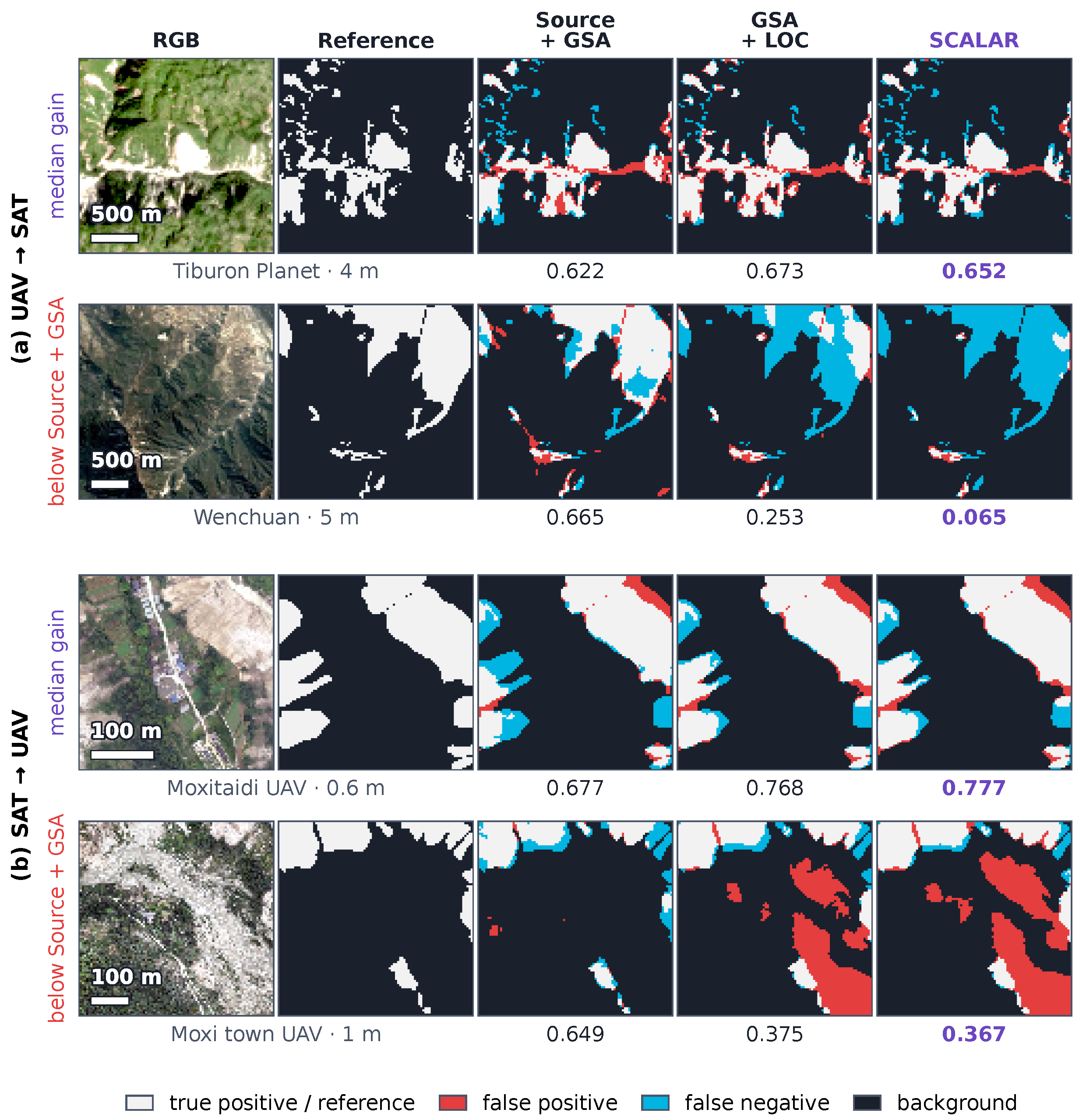
The qualitative examples in Figure A1 use the candidate tiles underlying the Figure 6 selection procedure: up to 40 randomly sampled tiles per target subset with 10–50% reference landslide pixels. For the displayed models, each direction shows the candidate closest to the median SCALAR-minus-anchored-source IoU difference and the candidate with the largest loss. The Wenchuan 5 m example falls from 0.665 to 0.065 IoU and the Moxi town 1 m example from 0.649 to 0.367, illustrating loss of true detections and increased false positives, respectively.
Figure A1.
Representative gains and negative-transfer examples in UAV-to-SAT (top two rows) and SAT-to-UAV (bottom two rows). Columns show RGB, reference labels, Source + GSA, GSA + LOC and SCALAR. The candidate-selection rule is given in the accompanying text. GSA + LOC and SCALAR are the seed-0 checkpoints retrained for the supplementary operating-point analysis (Table 5), not the checkpoints in Figure 6. Values below predictions are tile-level IoUs.
Appendix F. External Datasets and the Bijie Evaluation
GDCLD [31] uses scene-level GeoTIFFs from its test package, with nominal GSD from the geotransform. Events are absent from CAS; overlapping Palu is excluded, and the training/validation packages are unused. Scenes are tiled into 1024-pixel windows. SAT transfers to 0.5 m Map World scenes at anchor 0.5 m and ; UAV transfers to 3 m PlanetScope scenes at anchor 1 m and , both at seed 0. Auxiliary checks randomly halve each scene set. At threshold 0.5, transductive Source + GSA/SCALAR IoUs are 0.224/0.282 for Lushan_1 (Lushan 2022, 133 tiles) and 0.286/0.379 for Lushan_2 (Lushan 2022, 168 tiles), both at 0.5 m. For 3 m scenes they are 0.026/0.054 for Lushan_3 (Lushan 2022, 90 tiles), 0.086/0.073 for Mesetas (2019, 144 tiles), and 0.320/0.239 for West Sumatra (2022, 107 tiles). At 0.5 m the symmetric gate makes SCALAR identical to GSA + LOC.
GDCLD 0.5 m AP is 0.215/0.317/0.380 for native/anchored/full models (full equals LOC). At 3 m, native/anchored/LOC/full AP is 0.080/0.156/0.087/0.097. Anchored-teacher P/R at 0.5 is 0.55/0.35 and 0.16/0.58, respectively.
Bijie [32] contains 2773 RGB crops at 0.8 m in Guizhou: 770 masked landslide crops and 2003 non-landslide crops assigned empty masks. The available DEM is unused. Side lengths are 61–1239 pixels; median dimensions are approximately . The plan/hash were recorded on 22 October 2026 before download. An erratum corrected verbal margin direction without changing the listed SAT/UAV widths /. Before any model run, amendments added inductive splitting, dimension-based target-padding exclusion and seed scheduling. Padding exclusion followed inspection of crop dimensions.
Protocol C source partitions are reused. SAT source models are retrained at the rule-selected 0.6 m anchor; existing 1 m UAV sources are reused. CAS source-validation IoU selects checkpoints; target labels are reserved for evaluation. The seed-0 inductive split sorts and shuffles landslide/non-landslide groups separately, then assigns alternating indices (1387/1386 crops), with the exclusions in Section 3.2. A failed native-source inference on dimensions not divisible by 32 was rerun after edge-padding inputs and cropping logits back, without changing the model.
External runs use SegFormer-B2 and RGB. Bijie anchors are 0.6/1 m with ratios 1.33/0.8 for SAT/UAV transfer; anchored and adapted models use seeds 0–2, and native sources use seed 0. Target padding is excluded under the documented pre-run amendment. The prespecified primary contrast is SCALAR minus its matched anchored source; three-seed paired tests use two degrees of freedom and unadjusted exploratory p-values.
Table A7 retains every prescribed model/seed and secondary outcome. Adapted IoU, P/R and group metrics use final records of the source-validation-selected student; source metrics and AP use supplementary evaluation. Re-evaluated adapted IoU differs by less than 0.00010. Full-precision values determine means, sample deviations and paired increments (Table A7b); native seed 0 remains a fixed reference.
Table A7.
Bijie results by model and seed. IoU, precision (P) and recall (R) use threshold 0.5; AP uses scores across thresholds. All-crop metrics pool 2773 crops; LS IoU pools only the 770 landslide crops; background FP is the percentage of pixels predicted positive in the 2003 non-landslide crops. Native sources are evaluated at seed 0 only.
Appendix G. Supplementary Transfer and Comparator Controls
The within-platform GSA + LOC increments are +16.3/+21.5 points in UAV pairs and +2.8/+3.4 in SAT pairs; RSR adds , +0.7, and points at , 0.4, 8.3 and approximately 0.17.
Table A8 varies the GSD bands within the UAV and SAT platform groups. Each pair uses the frozen design and its rule-selected anchor; source models and adapted models are fitted for that pair. Source and target subsets have different region labels, but Wenchuan geographically contains the Longxi study area. Consequently, W3 and W4 have possible geographic overlap between Longxi SAT and the Wenchuan subset (178 Wenchuan target tiles in W3 and 160 Wenchuan source tiles in W4). Region labels alone do not establish spatial independence. The comparisons also change region and image collection, and therefore cannot isolate GSD as the sole cause of the performance changes.
Table A8.
Within-platform transfers across GSD bands. Panel (a) gives the source and target subsets, the anchor and the target-median-to-anchor ratio. Panel (b) gives seed-0 IoUs and zero-shot precision/recall of Source + GSA; increments are in IoU points. Each pair uses its own models.
Adaptive gates reach 0.483/0.498 IoU in SAT→UAV and 0.330/0.318 in UAV→SAT (FlexMatch-style/FreeMatch-style), versus anchored sources 0.355/0.344. The former recover much of LOC’s benefit; the latter have higher recall and lower precision.
The fixed-gate scan (Table A10) raises MIC-style SAT→UAV from 0.305 to 0.328 at gate 0.80; other pairs improve at most 0.003. All tested settings remain below same-seed SCALAR.
Matched SAT→UAV seeds 1–4 give AP 0.614 for the source versus 0.488/0.493 for DACS/MIC; oracle IoUs are 0.468 versus 0.390/0.399. Inference thresholds cannot recover the ranking loss. Comparator Otsu means span 0.304–0.396 versus matching-source 0.419. The loss of ranking quality persists across operating points.
Adaptive-gate controls use seed 0, fixed-gate scans seed 1, and operating-point analyses the matched seed sets stated in their tables. Benchmark defaults are unchanged.
Table A9.
Adaptive-confidence-gate controls in the reference loop (seed 0, IoU at 0.5). GSA + LOC and SCALAR use the supplementary analysis runs described in Section 3.4; these are not the original five-seed main-comparison summaries.
Table A10.
Confidence-gate sensitivity of DACS-style and MIC-style (seed 1). Entries show IoU at 0.5, with pixel AP in parentheses. The middle gate is the default of the present reference loop; all tested gates are shown.
Table A11.
Operating-point diagnostics. (a) Main-protocol seed-0 checkpoints, each held fixed across thresholds; prior denotes an EM-prior-matched quantile, and adapted checkpoints are the supplementary runs of Table 5. (b) Comparators and sources averaged over matching seed sets. Oracle thresholds use labels only for analysis; AP and oracle IoU use 1024 probability bins.
Appendix H. Module Controls and Teacher Diagnostics
Appendix H.1. Teacher Diagnostics
Retrospective teacher P/R at seed 0 is 0.89/0.37 and 0.47/0.56 for main SAT→UAV and UAV→SAT, and 0.55/0.35 and 0.16/0.58 for GDCLD 0.5/3 m. Under region hold-out, SAT→UAV under-detects on the pool (0.97/0.16) and held-out tiles (0.76/0.15); UAV→SAT over-predicts on the pool (0.43/0.55) but under-detects on evaluation tiles (0.71/0.43). Bijie teachers under-detect, with SAT P/R ranges 0.61–0.65/0.07–0.12 and UAV 0.53–0.55/0.16–0.22. Under-detection accompanies larger gains in these settings; over-prediction accompanies a smaller gain, no resolved gain or a loss. This label-based association combines seed-0 diagnostics and single- or multi-seed outcomes; it is retrospective, not causal or a validated deployment rule. The 1 m sensitivity run and additional backbones are outside this comparison.
Table A12 summarises the available seed-0 training logs matched to the backbone comparison in Table 7: all twelve SCALAR runs and nine GSA + LOC runs, each with ten adaptation epochs. GSA + LOC logs are unavailable for the remaining three backbone–direction combinations in this audit. Thresholds are on the probability scale; they are not logit-distribution summaries. The retention statistic is the batch mean of the fraction of all target training-grid pixels passing the relative gate, averaged within an epoch and then minimised across the ten epochs. It is measured before ClassMix, includes background and the target padding retained by the original protocol, and is not restricted to the 256-tile threshold-estimation pool. It neither estimates class-specific retention nor verifies pseudo-label accuracy.
Across these 21 runs, first/last thresholds span 0.059–0.237/0.154–0.398 and minimum epoch-mean retention spans 0.894–0.983. Fixed logit margins can affect backbones differently; normalisation by a robust measure of logit spread remains an untested extension.
HRNet UAV→SAT LOC has the lowest minimum retention (0.894) without clipping; its SCALAR counterpart has 0.932 retention and two epochs at 0.020. The other twenty runs do not clip. Historical bin-occupancy uncertainty is documented in Appendix C.
Table A12.
Threshold and retention diagnostics for available seed-0 runs in Table 7. and are first- and last-epoch probability thresholds; is the minimum epoch-mean gate-retention ratio; clipping counts epochs whose threshold reaches 0.020 or 0.980.
On the five backbones excluded from development, RSR exceeds LOC in eight of ten seed-0 comparisons (five SAT→UAV, three UAV→SAT), four by over two points. SegFormer-B0’s UAV→SAT recovery still falls below its anchored source.
For , RSR admits previously ignored positives and removes uncertain background labels. On the Longxi UAV tile in Figure 4c, retained pseudo-label recall increases from 60.2% to 65.5%, while precision decreases from 97.6% to 96.7%.
Retained-positive recall uses all reference landslide pixels, including rejected pixels, as its denominator; precision uses all retained positive pseudo-labels.
A separate five-seed diagnostic fixes each initial GSA teacher’s scores and LOC boundary on the 256-tile target pool and changes only the retention gate. In SAT→UAV, RSR increased retained-positive recall from to , while precision decreased from to . In UAV→SAT, recall decreased from to , while precision increased from to . Values are means ± sample standard deviations across five teachers.
The ratio of mean teacher probability to the true pool landslide fraction began at in UAV→SAT. The SAT→UAV symmetric-LOC teacher began below one, at .
Figure A2b,c tracks teacher probability drift. Before epoch 10, the mean ratio to the true pool fraction was 1.566 under symmetric LOC and 1.323 under RSR for UAV→SAT; the SAT→UAV ratios were 0.732 and 0.846. RSR reduced the absolute deviation from one by 43.0% and 42.5%, respectively.
Figure A2.
LOC calibration and teacher dynamics across five seeds. (a) Matched student IoUs; thick lines connect means. (b,c) Teacher mean probability relative to the true landslide fraction of the fixed pool, measured before each epoch. Bands show sample standard deviations; epoch 1 is the initial teacher. Reference labels are used only for evaluation and diagnostics.
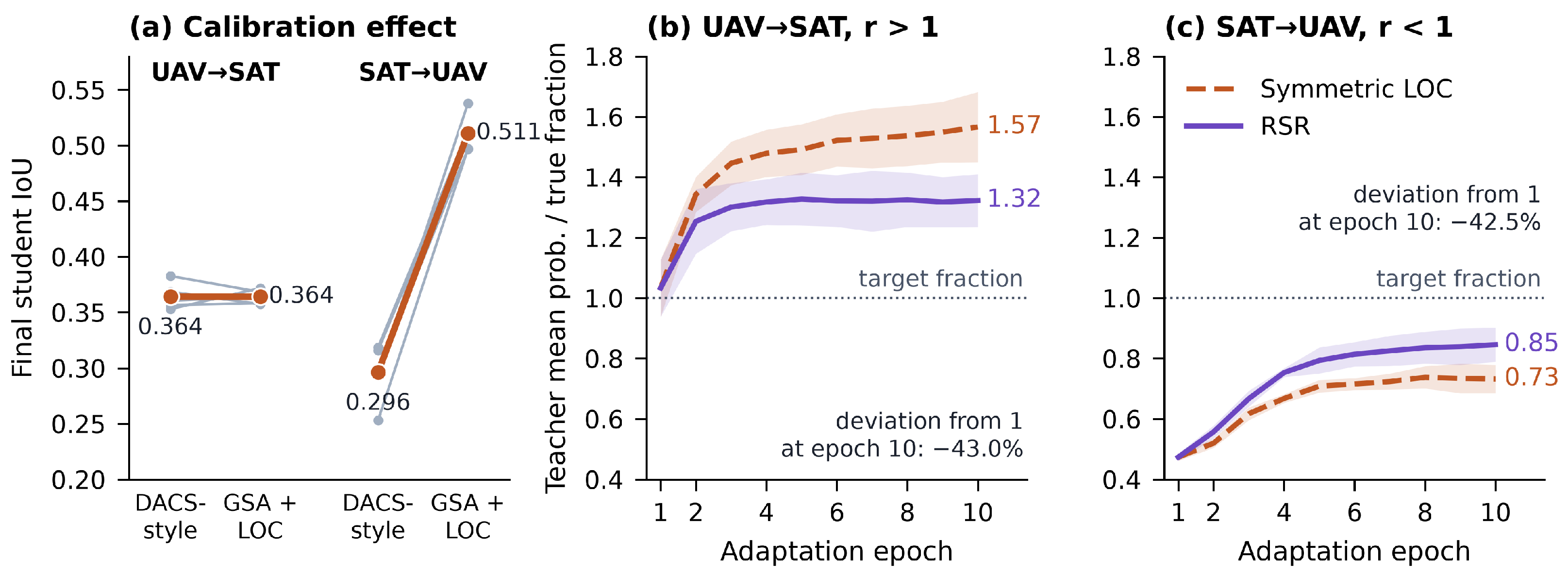
Appendix H.2. Module and Sensitivity Controls
Table A13.
Module controls at threshold 0.5. Panels (a–c) use seed 0; the reverse gate swaps Equation (6) widths. Panel (d) gives five-seed SAT-to-UAV mean ± sample standard deviation. Panel (e) uses the supplementary seed-0 checkpoints of Table 5, distinct from (c). Width pairs are in units of for and reversed for ; the asterisk marks the reference setting used in the RSR experiments.
GSA. The seed-0 scale controls in Table A13a use source labels only, so their differences precede pseudo-label adaptation. GSA reached 0.344 and 0.355, whereas random scale jitter over 0.5–2.0, sampled uniformly in log scale, reached 0.120 and 0.177. Generic scale augmentation did not reproduce the benefit of metadata-guided anchoring.
The seed-0 axis/gate controls show an 18.2-point LOC advantage over probability-axis Otsu in SAT→UAV, but a 2.1-point disadvantage in UAV→SAT (Table A13b). The latter has not been replicated; the five-seed boundary-only comparison is reported in panel (d) and Section 3.5.
Reversing RSR gives lower IoU than symmetric LOC in both directions (Table A13c); the supplementary width sweep and additional variants use their separately identified checkpoints.
The metadata-selected anchors achieved the highest IoUs among the source-supervised anchor checks (Table A14).
Table A14.
Sensitivity checks. (a) Seed-0 IoU at threshold 0.5; asterisks mark defaults and each block identifies its model. The cap check changes inference only and was not evaluated in SAT-to-UAV; retrained-bound and metadata-perturbation checks are in Table A3. (b) Domain-ratio definitions with the anchor and partitions fixed: triples denote tile-count/nominal-footprint/landslide-area weighting. The last requires reference labels.
The fixed GSA model changes by about 0.1 IoU points when its inference cap rises from to or (Table A14a). Uniform native-model enlargement instead gives 0.229, 0.291, 0.321 and 0.344 at , , and . These seed-0 UAV→SAT checks compare native-trained uniform resizing with GSA-trained, per-tile metadata resizing; both use threshold 0.5.
Table A3 shows lower UAV-to-SAT IoU with narrower [1/2, 1.4] bounds and no consistent improvement with wider bounds. At the 0.5 m SAT-to-UAV anchor, lower bounds are inactive; the equivalent-setting runs differ by 1.17 points, which is not a lower-bound effect.
For SCALAR, factors 0.7/1.4 alter IoU by less than 2.5 points; halving GSD loses 4.4/0.6 points and doubling changes it by +1.1/ in UAV-to-SAT/SAT-to-UAV. Source + GSA loses 3.7/5.9 points at factor 0.7. These are fixed-model inference effects (Table A3).
The single-seed asymmetric-width sweep exceeds the reference RSR setting in SAT→UAV by 2.3 points (Table A13e); it describes sensitivity without selecting a new optimum.
The symmetric-margin scan favours the default in SAT→UAV and in UAV→SAT. Pool-size ranges are 1.3/2.2 points, with neither maximum at ; defaults are unchanged. These single-seed ranges are descriptive.
Continuous per-tile asymmetry and a training-only reliability head did not provide a consistent improvement over RSR (Table A15). Their combined five-seed configuration reached and , below the corresponding RSR means of and ; no significant difference was claimed.
Selected plugins also varied by direction. Adding 64-pixel masked consistency to GSA + LOC gave 0.337 and 0.539 in UAV→SAT and SAT→UAV, respectively, whereas adding rare-class sampling gave 0.370 and 0.500. These were seed-0 checks.
Table A15.
Additional margin and reliability variants under GSA. All values are landslide IoU at probability 0.5. Entries with are seed-0 results; the combined refinements report five-seed mean ± sample standard deviation.
Appendix I. Aggregation and Evaluation Uncertainty
Run-level paired two-sided t-tests use unrounded differences, with four degrees of freedom for five seeds. The 14 region-held-out contrasts form one Holm family; each direction’s three sequential increments form another. The two-IoU-point convention is descriptive, not a significance criterion. Fixed-checkpoint bootstrap intervals below quantify evaluation uncertainty separately from training-run variation.
Equal-weight summaries first average the subset or dataset-region IoUs within each run and then report the mean and sample standard deviation across seeds 0–4 (Table A16). Region means use direct region-level IoUs, not an average of subset means within a region. SAT-to-UAV has seven subsets and three region labels; UAV-to-SAT has nine subsets and eight region labels. Longxi and Wenchuan remain separate dataset labels in this descriptive equal-weight summary and are not treated as independent spatial regions. They are merged for the bootstrap below.
SAT-to-UAV ordering is unchanged by equal weighting. In UAV-to-SAT, subset-equal LOC/SCALAR both round to 0.308 (SCALAR slightly lower unrounded), and region-equal values are 0.306/0.307. The full method’s small fine-to-coarse advantage therefore depends on aggregation weights.
Table A16.
Main-protocol aggregation at threshold 0.5, using the matching five runs for each model configuration. Entries are mean ± sample standard deviation; four decimals distinguish the near-identical equal-weight means. Three-decimal statements in the text use the unrounded means rather than rounding these entries again. The native source, anchored source and SCALAR correspond to Table 3; GSA + LOC is the five-seed configuration in Table 6.
For 2000 paired bootstrap replicates (Table A17), confusion counts are pooled before computing IoU and model differences. The fixed checkpoints are those of the supplementary operating-point analysis. Geographic clusters number seven in UAV-to-SAT after Longxi/Wenchuan merging, and three in SAT-to-UAV. Marginal 95% percentile intervals are separate from multiplicity-adjusted, across-seed tests.
Cluster intervals include zero for UAV-to-SAT LOC, RSR and full-adaptation increments, and SAT-to-UAV RSR. Both GSA increments and SAT-to-UAV LOC/full increments exclude zero. Narrower tile intervals do not account for neighbour dependence; neither scheme includes training variation. Few clusters limit population inference.
Table A17.
Fixed-checkpoint bootstrap at threshold 0.5 (2000 replicates). The checkpoints are those of Table 5 and Table A11, including GSA + LOC and SCALAR retrained for that supplementary analysis, not the five-seed statistics of Table 6. Individual-model rows use IoU units; difference rows use IoU points.
References
- Yang, Z.Q.; Qi, W.W.; Xu, C.; Shao, X.Y. Exploring deep learning for landslide mapping: A comprehensive review. China Geol. 2024, 7, 330–350. [Google Scholar] [CrossRef] [Scilit]
- Ma, Y.; Chen, S.; Ermon, S.; Lobell, D.B. Transfer learning in environmental remote sensing. Remote Sens. Environ. 2024, 301, 113924. [Google Scholar] [CrossRef] [Scilit]
- Song, W.; Liu, S.; Wu, S.; Liao, C.; Wu, Z.; Li, S.; Zheng, X.; Duan, Y. SC-Net: Structural Constrained Contrastive Learning for Landslide Extraction Toward Power Transmission Corridor Safety Monitoring. Remote Sens. 2026, 18, 2216. [Google Scholar] [CrossRef] [Scilit]
- Ploton, P.; Mortier, F.; Réjou-Méchain, M.; Barbier, N.; Picard, N.; Rossi, V.; Dormann, C.; Cornu, G.; Viennois, G.; Bayol, N.; et al. Spatial validation reveals poor predictive performance of large-scale ecological mapping models. Nat. Commun. 2020, 11, 4540. [Google Scholar] [CrossRef] [Scilit]
- Roberts, D.R.; Bahn, V.; Ciuti, S.; Boyce, M.S.; Elith, J.; Guillera-Arroita, G.; Hauenstein, S.; Lahoz-Monfort, J.J.; Schröder, B.; Thuiller, W.; et al. Cross-validation strategies for data with temporal, spatial, hierarchical, or phylogenetic structure. Ecography 2017, 40, 913–929. [Google Scholar] [CrossRef] [Scilit]
- Ghorbanzadeh, O.; Xu, Y.; Ghamisi, P.; Kopp, M.; Kreil, D. Landslide4Sense: Reference Benchmark Data and Deep Learning Models for Landslide Detection. IEEE Trans. Geosci. Remote Sens. 2022, 60, 1–17. [Google Scholar] [CrossRef] [Scilit]
- Ghorbanzadeh, O.; Xu, Y.; Zhao, H.; Wang, J.; Zhong, Y.; Zhao, D.; Zang, Q.; Wang, S.; Zhang, F.; Shi, Y.; et al. The Outcome of the 2022 Landslide4Sense Competition: Advanced Landslide Detection From Multisource Satellite Imagery. IEEE J. Sel. Top. Appl. Earth Obs. Remote Sens. 2022, 15, 9927–9942. [Google Scholar] [CrossRef] [Scilit]
- Yang, Y.; Soatto, S. FDA: Fourier Domain Adaptation for Semantic Segmentation. In Proceedings of the IEEE/CVF Conference on Computer Vision and Pattern Recognition, Virtual, 13–19 June 2020; pp. 4085–4095. [Google Scholar]
- Vu, T.H.; Jain, H.; Bucher, M.; Cord, M.; Pérez, P. ADVENT: Adversarial Entropy Minimization for Domain Adaptation in Semantic Segmentation. In Proceedings of the IEEE/CVF Conference on Computer Vision and Pattern Recognition, Long Beach, CA, USA, 15–20 June 2019; pp. 2517–2526. [Google Scholar]
- Tranheden, W.; Olsson, V.; Pinto, J.; Svensson, L. DACS: Domain Adaptation via Cross-Domain Mixed Sampling. In Proceedings of the IEEE/CVF Winter Conference on Applications of Computer Vision, Virtual, 5–9 January 2021; pp. 1379–1389. [Google Scholar]
- Hoyer, L.; Dai, D.; Van Gool, L. DAFormer: Improving Network Architectures and Training Strategies for Domain-Adaptive Semantic Segmentation. In Proceedings of the IEEE/CVF Conference on Computer Vision and Pattern Recognition, New Orleans, LA, USA, 18–24 June 2022; pp. 9924–9935. [Google Scholar]
- Hoyer, L.; Dai, D.; Wang, H.; Van Gool, L. MIC: Masked Image Consistency for Context-Enhanced Domain Adaptation. In Proceedings of the IEEE/CVF Conference on Computer Vision and Pattern Recognition, Vancouver, BC, Canada, 18–22 June 2023; pp. 11721–11732. [Google Scholar]
- Xu, Q.; Ouyang, C.; Jiang, T.; Yuan, X.; Fan, X.; Cheng, D. MFFENet and ADANet: A robust deep transfer learning method and its application in high precision and fast cross-scene recognition of earthquake-induced landslides. Landslides 2022, 19, 1617–1647. [Google Scholar] [CrossRef] [Scilit]
- Zhang, X.; Yu, W.; Pun, M.O.; Shi, W. Cross-domain landslide mapping from large-scale remote sensing images using prototype-guided domain-aware progressive representation learning. ISPRS J. Photogramm. Remote Sens. 2023, 197, 1–17. [Google Scholar] [CrossRef] [Scilit]
- Chen, J.; Liu, J.; Zeng, X.; Zhou, S.; Sun, G.; Rao, S.; Guo, Y.; Zhu, J. A Cross-Domain Landslide Extraction Method Utilizing Image Masking and Morphological Information Enhancement. Remote Sens. 2025, 17, 1464. [Google Scholar] [CrossRef] [Scilit]
- Yang, J.; Ding, M.; Huang, W.; Xue, Q.; Dong, Y.; Chen, B.; Peng, L.; Zhang, F.; Li, Z. Cross-Domain Landslide Mapping in Remote Sensing Images Based on Unsupervised Domain Adaptation Framework. Remote Sens. 2026, 18, 286. [Google Scholar] [CrossRef] [Scilit]
- Yu, B.; Chen, W.; Wang, S.; Chen, F.; Muhamad, N.; Wang, L.; Zhang, X.; Wang, N. Towards transferrable landslide mapping: A style synchronization framework. GIScience Remote Sens. 2026, 63, 2668221. [Google Scholar] [CrossRef] [Scilit]
- Uribe-Ventura, R.; Viveen, W.; Pineda-Ancco, F.; Beltrán-Castañon, C. GeoNeXt: Efficient landslide mapping using a pre-trained ConvNeXt V2 encoder with a PSA-ASPP decoder. Artif. Intell. Geosci. 2025, 6, 100172. [Google Scholar] [CrossRef] [Scilit]
- Reed, C.J.; Gupta, R.; Li, S.; Brockman, S.; Funk, C.; Clipp, B.; Keutzer, K.; Candido, S.; Uyttendaele, M.; Darrell, T. Scale-MAE: A Scale-Aware Masked Autoencoder for Multiscale Geospatial Representation Learning. In Proceedings of the IEEE/CVF International Conference on Computer Vision, Paris, France, 2–6 October 2023; pp. 4088–4099. [Google Scholar]
- Tang, M.; Cozma, A.; Georgiou, K.; Qi, H. Cross-Scale MAE: A Tale of Multiscale Exploitation in Remote Sensing. In Proceedings of the Advances in Neural Information Processing Systems, New Orleans, LA, USA, 10–16 December 2023; Volume 36, pp. 20054–20066. [Google Scholar] [CrossRef] [Scilit]
- Saerens, M.; Latinne, P.; Decaestecker, C. Adjusting the Outputs of a Classifier to New a Priori Probabilities: A Simple Procedure. Neural Comput. 2002, 14, 21–41. [Google Scholar] [CrossRef] [Scilit]
- Lipton, Z.C.; Wang, Y.X.; Smola, A.J. Detecting and Correcting for Label Shift with Black Box Predictors. In Proceedings of the 35th International Conference on Machine Learning, Stockholm, Sweden, 10–15 July 2018; Volume 80, pp. 3122–3130. [Google Scholar]
- Liu, Y.; Deng, J.; Tao, J.; Chu, T.; Duan, L.; Li, W. Undoing the Damage of Label Shift for Cross-Domain Semantic Segmentation. In Proceedings of the IEEE/CVF Conference on Computer Vision and Pattern Recognition, New Orleans, LA, USA, 18–24 June 2022; pp. 7042–7052. [Google Scholar]
- Zou, Y.; Yu, Z.; Vijaya Kumar, B.V.K.; Wang, J. Unsupervised Domain Adaptation for Semantic Segmentation via Class-Balanced Self-training. In Proceedings of the Computer Vision—ECCV 2018, Munich, Germany, 8–14 September 2018; Volume 11207, pp. 297–313. [Google Scholar] [CrossRef] [Scilit]
- Iqbal, J.; Masood, A.; Sultani, W.; Ali, M. Leveraging topology for domain adaptive road segmentation in satellite and aerial imagery. ISPRS J. Photogramm. Remote Sens. 2023, 206, 106–117. [Google Scholar] [CrossRef] [Scilit]
- Tarvainen, A.; Valpola, H. Mean teachers are better role models: Weight-averaged consistency targets improve semi-supervised deep learning results. In Proceedings of the Advances in Neural Information Processing Systems, Long Beach, CA, USA, 4–9 December 2017; Volume 30, pp. 1195–1204. [Google Scholar]
- Olsson, V.; Tranheden, W.; Pinto, J.; Svensson, L. ClassMix: Segmentation-Based Data Augmentation for Semi-Supervised Learning. In Proceedings of the IEEE/CVF Winter Conference on Applications of Computer Vision, Virtual, 5–9 January 2021; pp. 1369–1378. [Google Scholar]
- Otsu, N. A Threshold Selection Method from Gray-Level Histograms. IEEE Trans. Syst. Man. Cybern. 1979, 9, 62–66. [Google Scholar] [CrossRef] [Scilit]
- Kurita, T.; Otsu, N.; Abdelmalek, N. Maximum likelihood thresholding based on population mixture models. Pattern Recognit. 1992, 25, 1231–1240. [Google Scholar] [CrossRef] [Scilit]
- Xu, Y.; Ouyang, C.; Xu, Q.; Wang, D.; Zhao, B.; Luo, Y. CAS Landslide Dataset: A Large-Scale and Multisensor Dataset for Deep Learning-Based Landslide Detection. Sci. Data 2024, 11, 12. [Google Scholar] [CrossRef] [Scilit]
- Fang, C.; Fan, X.; Wang, X.; Nava, L.; Zhong, H.; Dong, X.; Qi, J.; Catani, F. A globally distributed dataset of coseismic landslide mapping via multi-source high-resolution remote sensing images. Earth Syst. Sci. Data 2024, 16, 4817–4842. [Google Scholar] [CrossRef] [Scilit]
- Ji, S.; Yu, D.; Shen, C.; Li, W.; Xu, Q. Landslide detection from an open satellite imagery and digital elevation model dataset using attention boosted convolutional neural networks. Landslides 2020, 17, 1337–1352. [Google Scholar] [CrossRef] [Scilit]
- Xie, E.; Wang, W.; Yu, Z.; Anandkumar, A.; Alvarez, J.M.; Luo, P. SegFormer: Simple and Efficient Design for Semantic Segmentation with Transformers. In Proceedings of the Advances in Neural Information Processing Systems, Online, 6–14 December 2021; Volume 34, pp. 12077–12090. [Google Scholar]
- Ronneberger, O.; Fischer, P.; Brox, T. U-Net: Convolutional Networks for Biomedical Image Segmentation. In Proceedings of the Medical Image Computing and Computer-Assisted Intervention—MICCAI 2015, Munich, Germany, 5–9 October 2015; Volume 9351, pp. 234–241. [Google Scholar] [CrossRef] [Scilit]
- Chen, L.C.; Zhu, Y.; Papandreou, G.; Schroff, F.; Adam, H. Encoder-Decoder with Atrous Separable Convolution for Semantic Image Segmentation. In Proceedings of the Computer Vision—ECCV 2018, Munich, Germany, 8–14 September 2018; Volume 11211, pp. 833–851. [Google Scholar] [CrossRef] [Scilit]
- He, K.; Zhang, X.; Ren, S.; Sun, J. Deep Residual Learning for Image Recognition. In Proceedings of the IEEE Conference on Computer Vision and Pattern Recognition, Las Vegas, NV, USA, 27–30 June 2016; pp. 770–778. [Google Scholar]
- Xiao, T.; Liu, Y.; Zhou, B.; Jiang, Y.; Sun, J. Unified Perceptual Parsing for Scene Understanding. In Proceedings of the Computer Vision—ECCV 2018, Munich, Germany, 8–14 September 2018; Volume 11209, pp. 432–448. [Google Scholar] [CrossRef] [Scilit]
- Woo, S.; Debnath, S.; Hu, R.; Chen, X.; Liu, Z.; Kweon, I.S.; Xie, S. ConvNeXt V2: Co-Designing and Scaling ConvNets With Masked Autoencoders. In Proceedings of the IEEE/CVF Conference on Computer Vision and Pattern Recognition, Vancouver, BC, Canada, 18–22 June 2023; pp. 16133–16142. [Google Scholar]
- Wang, J.; Sun, K.; Cheng, T.; Jiang, B.; Deng, C.; Zhao, Y.; Liu, D.; Mu, Y.; Tan, M.; Wang, X.; et al. Deep High-Resolution Representation Learning for Visual Recognition. IEEE Trans. Pattern Anal. Mach. Intell. 2021, 43, 3349–3364. [Google Scholar] [CrossRef] [Scilit]
- Meena, S.R.; Soares, L.P.; Grohmann, C.H.; van Westen, C.; Bhuyan, K.; Singh, R.P.; Floris, M.; Catani, F. Landslide detection in the Himalayas using machine learning algorithms and U-Net. Landslides 2022, 19, 1209–1229. [Google Scholar] [CrossRef] [Scilit]
- Luo, M.; Ji, S. Cross-spatiotemporal land-cover classification from VHR remote sensing images with deep learning based domain adaptation. ISPRS J. Photogramm. Remote Sens. 2022, 191, 105–128. [Google Scholar] [CrossRef] [Scilit]
- Zhao, Q.; Lyu, S.; Zhao, H.; Liu, B.; Chen, L.; Cheng, G. Self-training guided disentangled adaptation for cross-domain remote sensing image semantic segmentation. Int. J. Appl. Earth Obs. Geoinf. 2024, 127, 103646. [Google Scholar] [CrossRef] [Scilit]
- Hoyer, L.; Dai, D.; Van Gool, L. HRDA: Context-Aware High-Resolution Domain-Adaptive Semantic Segmentation. In Proceedings of the Computer Vision—ECCV 2022, Tel Aviv, Israel, 23–27 October 2022; Volume 13690, pp. 372–391. [Google Scholar] [CrossRef] [Scilit]
- Zhang, P.; Zhang, B.; Zhang, T.; Chen, D.; Wang, Y.; Wen, F. Prototypical Pseudo Label Denoising and Target Structure Learning for Domain Adaptive Semantic Segmentation. In Proceedings of the IEEE/CVF Conference on Computer Vision and Pattern Recognition, Virtual, 19–25 June 2021; pp. 12414–12424. [Google Scholar]
- Huang, W.; Shi, Y.; Xiong, Z.; Zhu, X.X. Decouple and weight semi-supervised semantic segmentation of remote sensing images. ISPRS J. Photogramm. Remote Sens. 2024, 212, 13–26. [Google Scholar] [CrossRef] [Scilit]
- Meyer, H.; Pebesma, E. Machine learning-based global maps of ecological variables and the challenge of assessing them. Nat. Commun. 2022, 13, 2208. [Google Scholar] [CrossRef] [Scilit]
- Zhang, B.; Wang, Y.; Hou, W.; Wu, H.; Wang, J.; Okumura, M.; Shinozaki, T. FlexMatch: Boosting Semi-Supervised Learning with Curriculum Pseudo Labeling. In Proceedings of the Advances in Neural Information Processing Systems, Online, 6–14 December 2021; Volume 34, pp. 18408–18419. [Google Scholar]
- Wang, Y.; Chen, H.; Heng, Q.; Hou, W.; Fan, Y.; Wu, Z.; Wang, J.; Savvides, M.; Shinozaki, T.; Raj, B.; et al. FreeMatch: Self-adaptive Thresholding for Semi-supervised Learning. In Proceedings of the International Conference on Learning Representations, Kigali, Rwanda, 1–5 May 2023. [Google Scholar]
- Loshchilov, I.; Hutter, F. Decoupled Weight Decay Regularization. In Proceedings of the International Conference on Learning Representations, New Orleans, LA, USA, 6–9 May 2019. [Google Scholar]
- Zhuo, S.; Sim, T. Defocus map estimation from a single image. Pattern Recognit. 2011, 44, 1852–1858. [Google Scholar] [CrossRef] [Scilit]
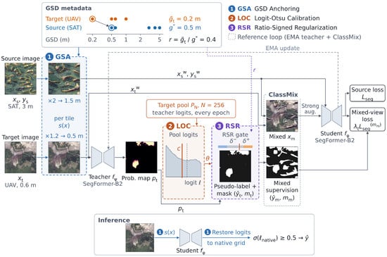
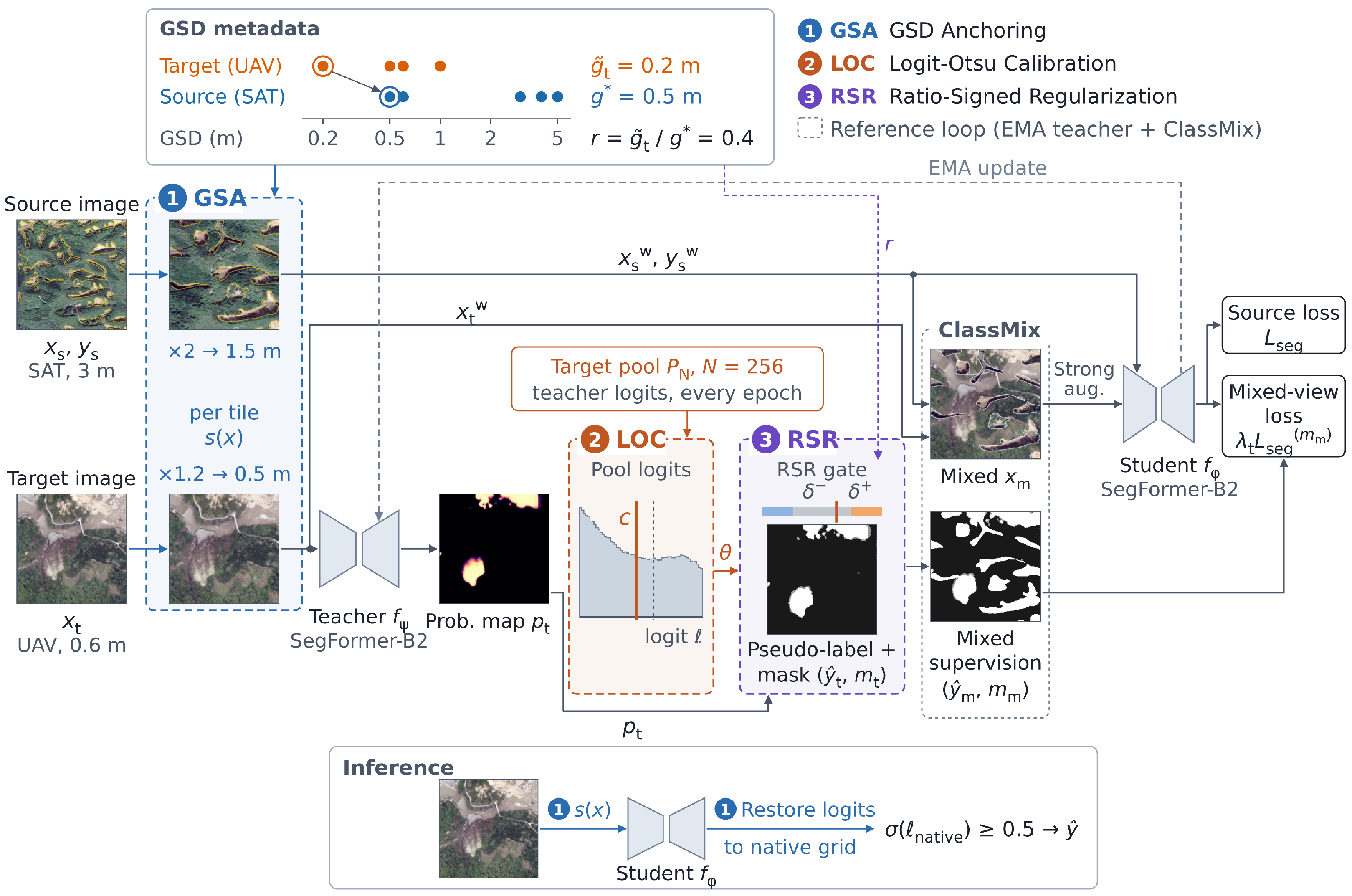
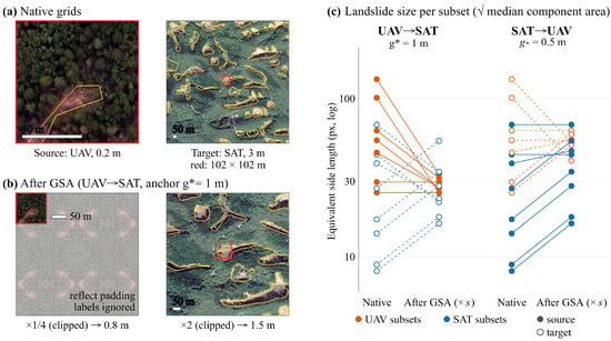
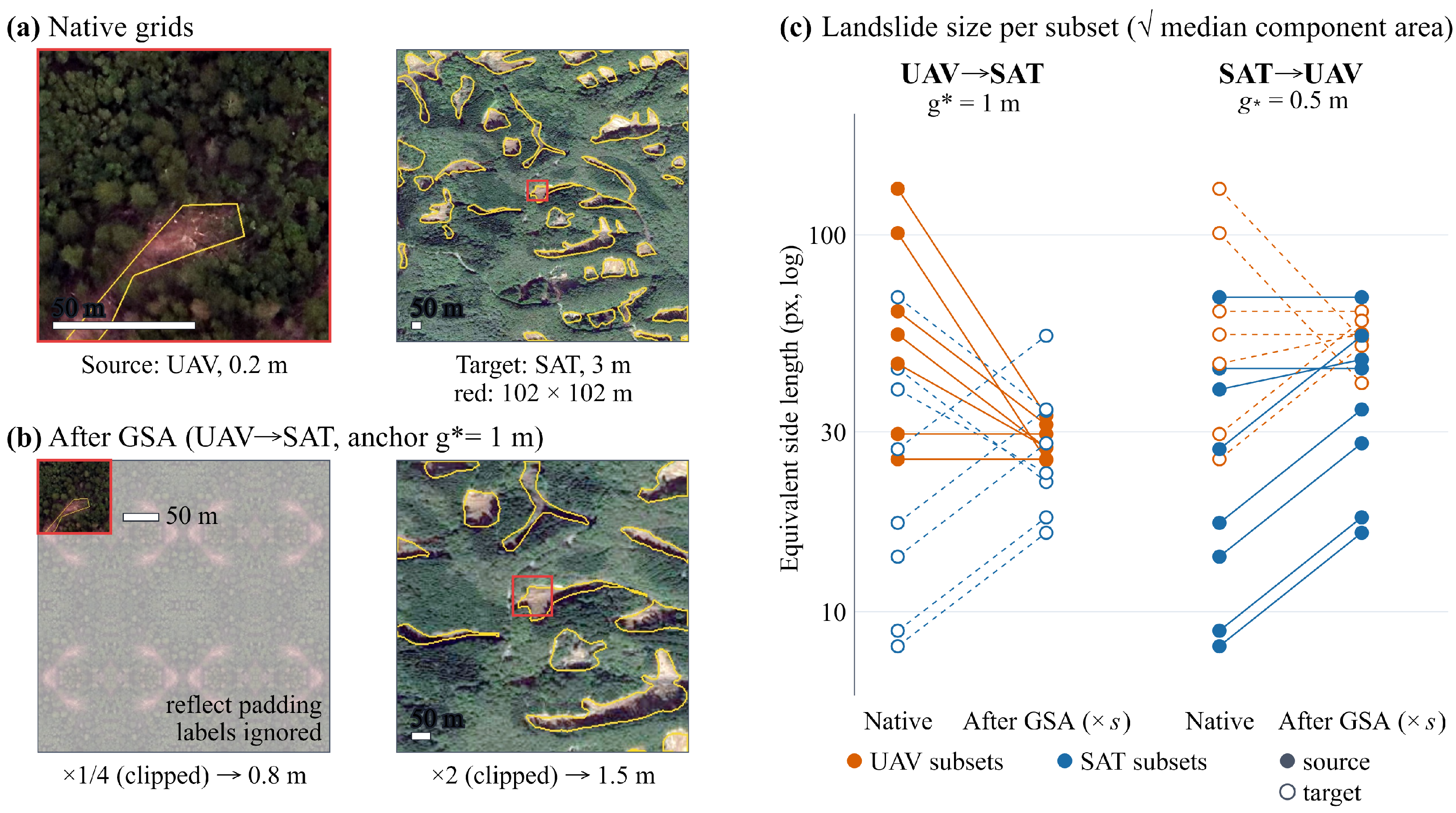
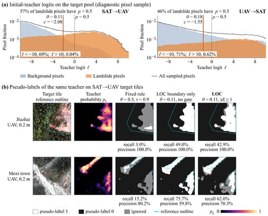
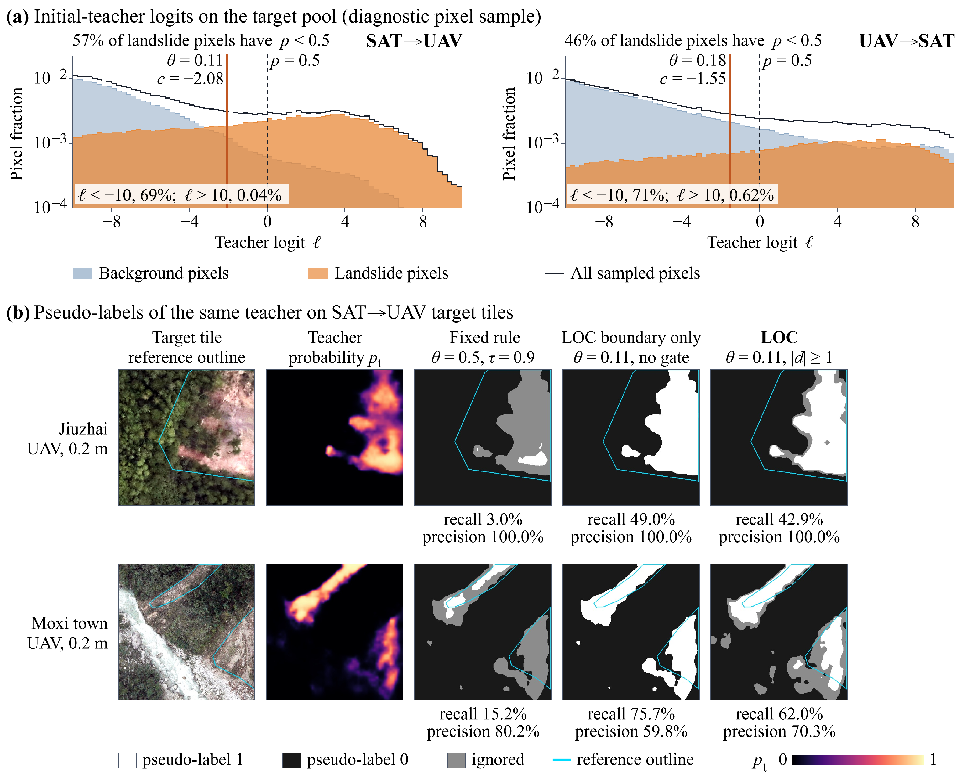
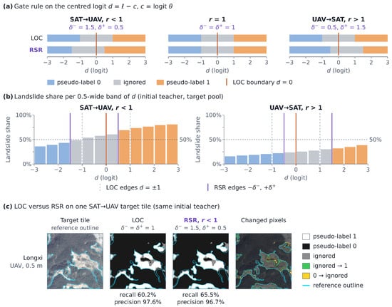
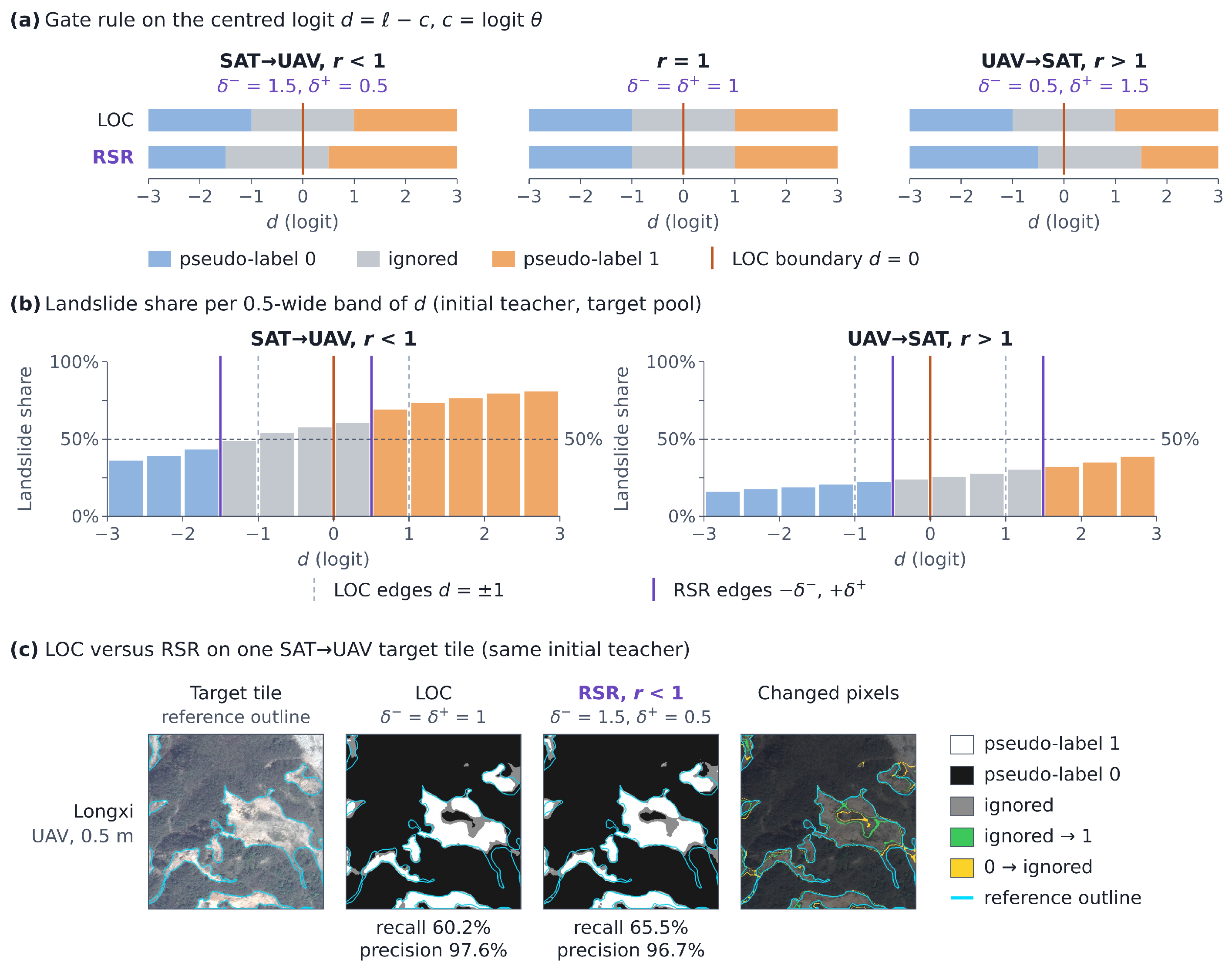
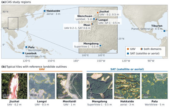
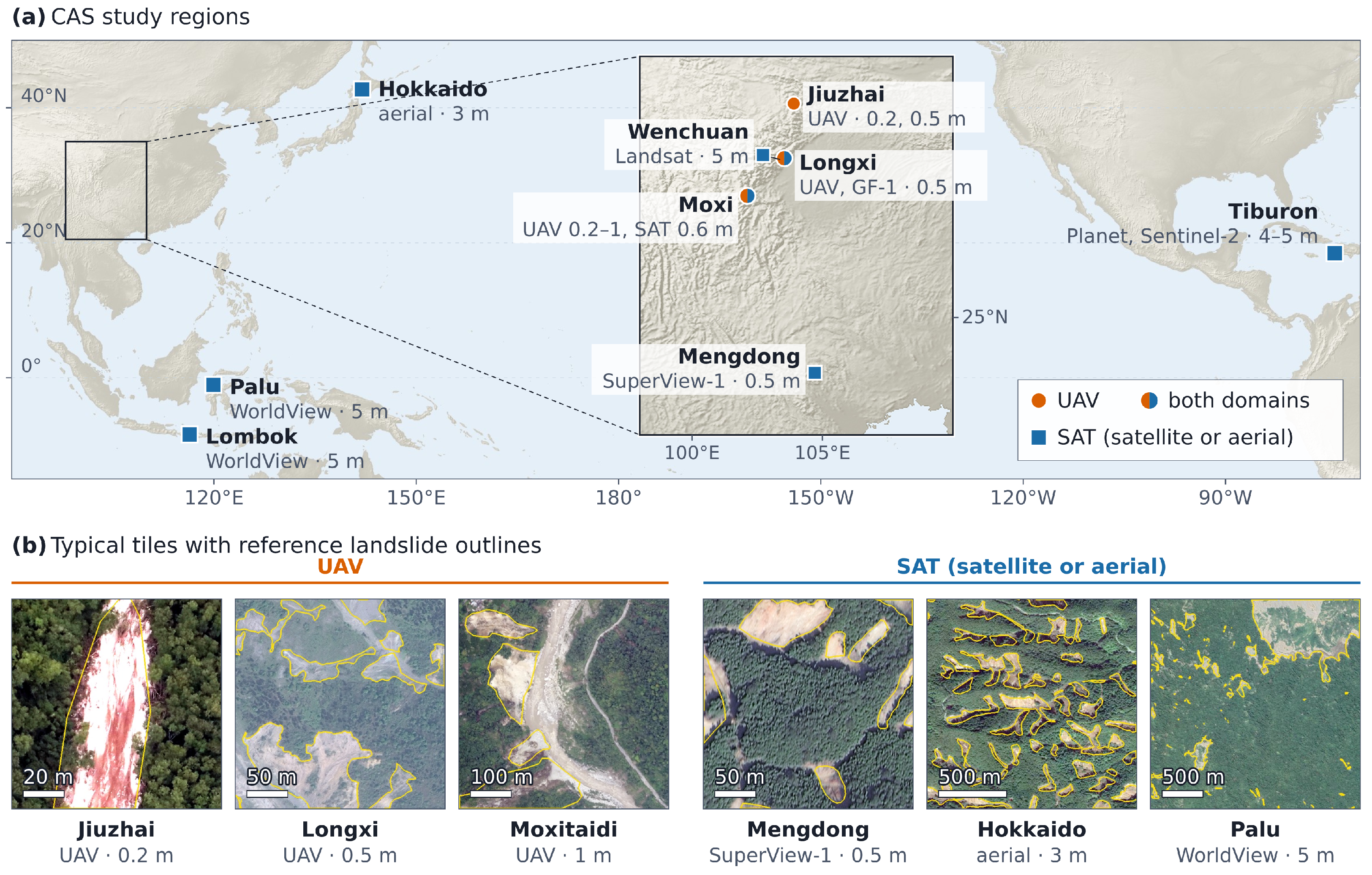
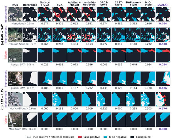
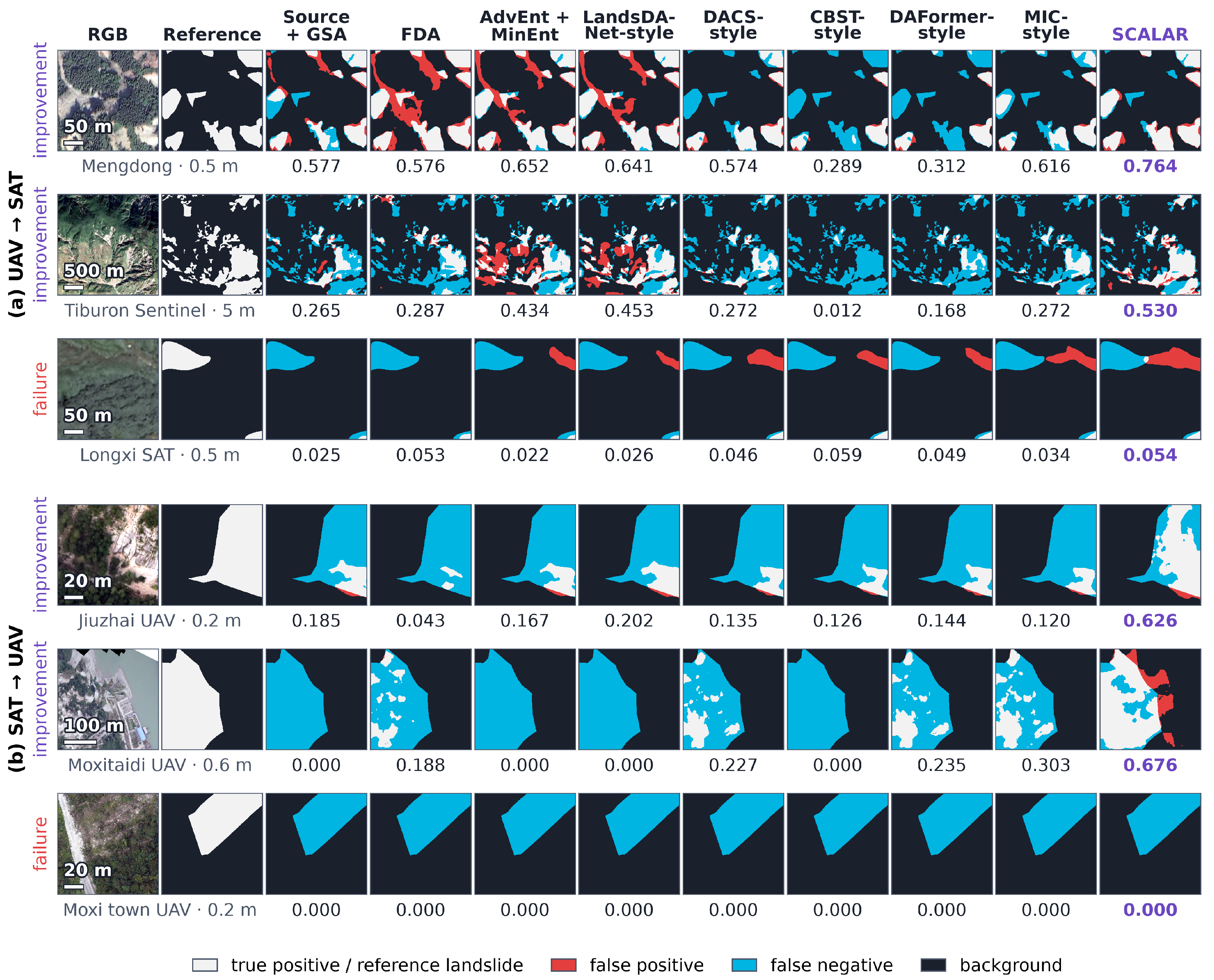

Disclaimer/Publisher’s Note: The statements, opinions and data contained in all publications are solely those of the individual author(s) and contributor(s) and not of MDPI and/or the editor(s). MDPI and/or the editor(s) disclaim responsibility for any injury to people or property resulting from any ideas, methods, instructions or products referred to in the content. |
© 2026 by the authors. Licensee MDPI, Basel, Switzerland. This article is an open access article distributed under the terms and conditions of the Creative Commons Attribution (CC BY) license.