


Highlights
What are the main findings?
- Quasi-biennial-range (20–36-month) stratospheric ozone variability exhibits differences among the examined pressure levels, with relatively enhanced tropical 20–36-month normalized power at 10 hPa.
- At 10 hPa, tropical quasi-biennial-range variability is evident across many tropical longitudes, with variations in normalized power among longitudes.
What are the implications of the main findings?
- Longitude-resolved diagnostics allow for longitude-dependent variability to be described alongside zonal-mean summaries.
- The AIRS-based results may inform further studies of possible links between quasi-biennial-range ozone variability, circulation, wave activity, and chemical processes.
Abstract
Stratospheric ozone exhibits quasi-biennial-range variability, whose spatial organization can differ among pressure levels and longitudes. We analyzed Aqua Atmospheric Infrared Sounder (AIRS) Version 7 monthly ozone observations from September 2002 to December 2025 at 50, 10, and 3 hPa. A Morlet wavelet analysis of standardized anomalies characterized the 20–36-month variability, with AR(1) Monte Carlo significance tests and complementary multiple-testing and uncertainty assessments. The tropical 10 hPa band showed relatively enhanced normalized power and widespread longitudinal support: 326 of 359 eligible longitudes remained significant after a within-level Benjamini–Hochberg adjustment of band-level tests. In the global 10 hPa grid-cell analysis, 6792 of 62,191 eligible cells passed the corresponding global Benjamini–Hochberg adjustment. Conditional block-bootstrap comparisons indicated differences in some predefined longitude-sector contrasts, whereas the confidence intervals for the 10-minus-50 hPa longitude-power coefficient-of-variation difference included zero. Regressions using NOAA CPC and KIT/FU Berlin QBO wind records indicated longitude-sector heterogeneity in the 10 hPa ozone–QBO regression associations using the 50 hPa wind index. The ERA5 temperature and low-wavenumber geopotential height patterns provided meteorological context, although the assessed ozone–ERA5 spatial alignments did not pass the adopted spatial-null tests. These findings offer a pressure-dependent, longitude-resolved description of quasi-biennial-range ozone variability and selected QBO-associated statistical relationships, without establishing a unique dynamical or chemical attribution.
1. Introduction
Stratospheric ozone varies across a wide range of temporal and spatial scales, and its distribution is influenced by atmospheric dynamics, transport processes, and photochemical reactions [1,2]. The characteristics of ozone variability differ with altitude and latitude, reflecting variations in the background atmospheric state and the processes controlling stratospheric composition. Characterizing the spatial and temporal organization of ozone variability can help describe its observed patterns and provide context for examining the processes that may contribute to them. In a broader upper-atmospheric context, Sheng et al. [3] reviewed dynamics, chemistry, and modeling in the aviation and aerospace transition zone (approximately 50–150 km), a region distinct from the three AIRS pressure levels analyzed here.
Quasi-biennial variability is a prominent feature of the tropical stratosphere, where the quasi-biennial oscillation (QBO) in equatorial zonal winds influences circulation and tracer transport [4]. Associated ozone variations have also been reported and are generally linked to QBO-related changes in transport, circulation, and chemical conditions [5]. However, ozone responses are neither vertically nor spatially uniform; their magnitude and structure vary with altitude and latitude due to differences in transport pathways, photochemical sensitivity, and background atmospheric conditions [1,5]. These differences motivate an examination of quasi-biennial-range ozone variability across pressure levels and spatial dimensions.
Previous studies have examined the vertical, meridional, and regional characteristics of ozone variability using long-term profile records and other observations [1]. More directly, Wang et al. [6] investigated zonally asymmetric QBO-related stratospheric ozone variations using satellite observations, ERA5 reanalysis, and model simulations. Their findings demonstrate that longitude-dependent ozone responses associated with the QBO have been investigated in previous work. Other studies have described spatially organized ozone variability or applied wavelet methods to satellite and ozonesonde records [7,8,9]. A complementary question is how the relative spectral contribution of a specified 20–36-month ozone component is distributed across longitude and pressure levels in AIRS retrievals, and how this distribution is affected by statistical uncertainty and sampling choices. The selected period range is therefore examined as a measure of quasi-biennial-range variability, without presuming that it uniquely identifies the dynamical QBO.
Long-term satellite observations provide broad spatial coverage for investigating stratospheric ozone variability [10]. The Atmospheric Infrared Sounder (AIRS) aboard NASA’s Aqua satellite has provided near-global atmospheric observations since 2002, including retrieved ozone profiles [10,11]. Published AIRS-related retrieval evaluations, product comparisons, and the Version 7 performance documentation provide useful context for interpreting the ozone record [11,12,13]. However, the reported pressure levels of an infrared retrieved profile are subject to vertical smoothing, and these sources do not establish independent, level-specific accuracy for the monthly 50, 10, and 3 hPa fields examined here. The AIRS record is therefore used to compare observed patterns at these reporting levels, with the retrieval characteristics and sampling limitations considered in the interpretation.
Characterizing the periodic variability in long-term satellite ozone records requires methods that accommodate changes in the strength and persistence of oscillatory signals over time. Continuous wavelet transform (CWT) analysis can describe the time–period structure of non-stationary variability [14], and wavelet approaches have been applied to total-column ozone and ozonesonde observations [8,9]. Because atmospheric series are autocorrelated, wavelet-power features also require evaluation against an appropriate red-noise background [14]. The present analysis combines Morlet wavelet estimates with AR(1)-based significance testing, multiple-testing assessments, and complementary uncertainty analyses.
In this study, we examine AIRS Version 7 monthly ozone observations from September 2002 to December 2025 at 50, 10, and 3 hPa, with particular attention to the predefined 20–36-month quasi-biennial range. The presence of variability within this period range is not, by itself, regarded as a dynamical QBO diagnosis. Two complementary equatorial zonal wind QBO records and ERA5 reanalysis fields are used to examine statistical associations and provide meteorological context, rather than to establish a unique causal mechanism. The study addresses four objectives:
(1) To characterize the latitude–period structure and pressure dependence of AIRS-derived ozone variability at the three selected reporting levels;
(2) To describe the longitude-resolved 20–36-month spectral organization of tropical ozone and assess the associated spatial contrasts, physical-unit variability, and sensitivity to the retrieval branch;
(3) To characterize the 10 hPa global distribution of 20–36-month band power and distinguish local statistical significance from multiple-testing-adjusted evidence, while documenting data completeness and grid-cell eligibility;
(4) To examine the longitudinal differences in the statistical associations between ozone variability and two QBO wind records, and to evaluate the complementary ERA5 meteorological patterns and temporal sensitivity.
Together, these analyses provide a longitude-resolved description of the observed ozone variability and its statistical context, without attributing the spatial patterns to a single dynamical or photochemical process.
2. Materials and Methods
2.1. AIRS-Only Satellite Ozone Observations and Quality Screening
This study used the AIRS-only Version 7 Level 3 monthly standard physical retrieval product (AIRS3STM, Version 7; https://doi.org/10.5067/UBENJB9D3T2H) distributed by the NASA Goddard Earth Sciences Data and Information Services Center (GES DISC). AIRS is a hyperspectral infrared sounder aboard NASA’s Aqua satellite [10]. Previous studies have evaluated AIRS’s retrieval performance [11,12], and a dedicated Version 7 report has provided further information on its ozone retrieval characteristics and averaging kernels [13]. These sources provide relevant background but do not independently validate the monthly tropical ozone fields analyzed here. The AIRS V7 Level 3 product definition, grid geometry, monthly aggregation, and sampling count conventions were checked against the product user guide in [15].
The analysis covered September 2002–December 2025 (280 calendar months). The AIRS-only product was used throughout to maintain a consistent retrieval configuration. The Level 3 product provides monthly fields on a 1° latitude–longitude grid and corresponding sampling count fields. The monthly record contains no duplicate or missing calendar months; this temporal completeness does not imply spatially complete valid ozone observations in every month.
Only ascending-node observations were retained for the analysis. The AIRS Level 3 product provides separate ascending- and descending-node quantities associated with different satellite overpass conditions. Rather than combining the two branches according to month-to-month availability, a fixed ascending-node configuration was used throughout the analysis period. Specifically, the analysis used the ascending-node ozone volume mixing ratio (VMR) variable (O3_VMR_A) and its corresponding count variable (O3_VMR_A_ct). Descending-node observations and availability-dependent combinations of ascending- and descending-node data were not included. The sensitivity to node selection is evaluated separately in Section 4.4 (Supplementary Figure S1 and Table S1).
Ozone variability was examined at three native AIRS pressure levels: 50, 10, and 3 hPa. No vertical interpolation was applied. Ozone was retained in VMR form during the initial data preparation. Anomaly construction and standardization were then performed as described in Section 2.2. These are standard product reporting levels of a vertically smoothed retrieved ozone profile and should not be interpreted as three vertically independent observations. The vertical information content depends on the retrieval averaging kernels and atmospheric conditions; level-specific sensitivity and uncertainty at 50, 10, and 3 hPa were not estimated for the monthly fields analyzed here [13].
Product fill values, non-finite values, and invalid numerical sentinels were treated as missing. Monthly ozone was retained only when the product-reported O3_VMR_A_ct input count met the study-defined threshold in Equation (1). The AIRS V7 Level 3 product guide describes the _ct fields as counts associated with inputs to gridded statistics [15], but does not establish that the monthly O3_VMR_A_ct value equals the number of distinct days with valid ozone daily means. Accordingly, the threshold is treated as an empirical screening criterion, not as an AIRS-prescribed quality flag or a verified fraction of valid observation days.
where Ndays denotes the number of calendar days in the corresponding month and ⌈·⌉ denotes rounding upward to the nearest integer. The threshold corresponds to a reported count of at least 7 for 28-day months and 8 for 29-, 30-, or 31-day months. This empirical screening criterion was applied consistently to the ascending-node fields. Values that failed the condition were treated as missing; no interpolation was applied at the raw monthly ingestion stage. The calendar-day scaling was used as a simple normalization for differences in month length rather than as an assumption that the reported counts represent distinct valid observation days.
O3_VMR_A_ct ≥ ⌈0.25 Ndays⌉
The monthly record covers all 280 calendar months from September 2002 to December 2025 without duplicate or missing months. This temporal completeness does not imply spatially complete valid ozone observations in every month. Under the study-defined 25% count screen, the median grid-cell valid-month fraction was approximately 0.996 at each pressure level, although spatial completeness varied by month. In particular, April 2024 contained no valid ascending-node ozone observations at the analyzed pressure levels after screening. This month was retained as missing during anomaly construction, with short-gap treatment applied only later to analysis-eligible time series as specified in Section 2.3.
To characterize the practical effect of the study-defined input-count screen, alternative thresholds of 50%, 67%, and 75% were compared with the adopted 25% criterion. The fractions of all possible grid-cell–month records retained were 93.43%, 74.51%, and 53.16%, respectively, compared with 98.06% under the 25% criterion. The 25% criterion was retained as a pragmatic, permissive screen to exclude records with very low reported input counts while preserving broad data availability. Because the product-reported count does not independently establish the number of distinct days with valid ozone observations, this criterion should not be interpreted as a validated measure of observational coverage. These comparisons characterize the raw-data retention and the trade-off with screening stringency; they do not establish that 25% is statistically optimal or that subsequent spectral estimates are insensitive to the threshold choice.
2.2. Temporal Anomaly Construction and Grid-Cell Standardization
Monthly ozone anomalies were constructed relative to calendar-month climatologies to remove the mean seasonal cycle from the screened AIRS ascending-node O3 VMR fields. For each grid cell and pressure level, a climatological mean was calculated independently for each calendar month using all available years that satisfied the monthly sampling criterion described in Section 2.1. A calendar-month climatology was retained only when at least 12 valid annual samples were available for that month. If this requirement was not satisfied for a particular month, only the climatology for that calendar month and the associated anomalies were treated as unavailable; valid climatologies and anomalies for the other calendar months at the same grid cell were retained.
For grid cell i and time t, the monthly ozone anomaly was defined as
where Oi(t) denotes the sampling-screened monthly ozone VMR, and is the climatological mean for the corresponding calendar month m(t). An anomaly was calculated only when both the monthly ozone observation and the corresponding calendar-month climatology were available.
Anomaly series were standardized independently at each grid cell and pressure level using all valid anomaly samples. The sample standard deviation was calculated from all available anomaly samples using n − 1 in the denominator. Grid cells were retained for standardization when at least 120 valid anomaly samples were available and the sample standard deviation exceeded 1 × 10⁻¹² in the native VMR units. The latter criterion was used as a numerical safeguard to exclude near-zero-variance series rather than as an AIRS retrieval-quality threshold. The standardized anomaly was defined as
where si is the sample standard deviation of the valid anomaly series at grid cell i. The resulting standardized anomalies are dimensionless and describe local ozone departures relative to the temporal variability in each grid cell.
Grid cells that did not satisfy the standardization requirements were treated as unavailable in subsequent grid-cell fields. Missing monthly values remained missing after anomaly construction and grid-cell standardization. Spatial aggregation, temporal completeness screening, and the treatment of short internal temporal gaps were performed as described in Section 2.3. Detrending and pre-CWT re-standardization were applied only after the final analysis-ready time series had been constructed, as described in Section 2.4.
2.3. Spatial Aggregation and Temporal Eligibility
The grid-cell standardized anomalies described in Section 2.2 were used to construct latitude-resolved and longitude-resolved monthly time series before wavelet analysis. For the latitude- and longitude-resolved analyses, eligibility was assessed at three levels: grid-cell standardization, spatial aggregation, and temporal completeness of the resulting time series. Spatial aggregation was performed using only grid cells that satisfied the standardization requirements, so that ineligible grid cells were not treated as expected observations in subsequent monthly coverage calculations. No spatial interpolation was applied.
For the latitude-resolved analysis, zonal-mean time series were constructed independently at each latitude and pressure level. A latitude was considered spatially eligible when at least 80% of its longitude grid cells met the grid-cell standardization criteria described in Section 2.2. For each eligible latitude and month, the zonal mean was calculated from the available standardized anomalies among these eligible longitude grid cells. The monthly value was retained only when at least 80% of the baseline eligible longitudes contained valid standardized anomalies. Thus, monthly coverage was evaluated relative to the longitude locations that met the Section 2.2 criteria, rather than relative to all 360 longitude grid cells.
For the longitude-resolved tropical analysis, standardized anomalies were aggregated over 10°S–10°N using cosine-latitude weighting while retaining the longitude dimension. The cosine-latitude weighting was used to account for unequal meridional grid-cell areas. For each longitude, baseline spatial eligibility was evaluated from the fraction of the total tropical latitude weight contributed by grid cells satisfying the standardization criteria. A longitude was retained when this eligible weight fraction was at least 80%. Here, Z(ϕ, λ, t) denotes the grid-cell standardized ozone anomaly defined in Equation (3), expressed at latitude ϕ, longitude λ, and month t. For each retained longitude and month, the tropical mean was calculated as
where Vλ,t denotes the set of standardization-eligible tropical latitude grid cells with valid standardized anomalies at longitude λ and month t. A monthly tropical longitude mean was retained only when the available cosine-latitude weight represented at least 80% of the baseline eligible tropical weight for that longitude.
After spatial aggregation, temporal eligibility was evaluated separately for each resulting one-dimensional time series. For the main latitude- and longitude-resolved analyses, time series were retained when they had at least 90% valid monthly coverage over the study record and no sequence of more than two consecutive missing months. A stricter 95% valid-month criterion, with the same maximum gap requirement, was retained as a sensitivity assessment.
Separately, uncertainty in the 10 hPa versus 50 hPa longitude-power coefficient-of-variation (CV) difference was assessed using paired temporal-block resampling, as described in Section 2.6 (Supplementary Figure S2 and Table S2).
For the complementary physical-unit comparison, the calendar-month climatology was first removed at each grid cell to obtain the un-standardized monthly ozone anomalies. These anomalies were then aggregated at each longitude over 10°S–10°N using cosine-latitude weights, subject to the tropical spatial-eligibility and monthly-coverage criteria described above (including the 80% relative-coverage requirement). The resulting longitude-resolved anomaly series were converted from VMR to ppmv and linearly detrended. The 20–36-month component was extracted using a third-order Butterworth band-pass filter with cutoff frequencies of 1/36 and 1/20 cycles month−1, applied using forward–backward filtering (sosfiltfilt). The RMS was calculated after excluding the first and last 36 months of the filtered series, leaving the central 208 months (September 2005–December 2022) of the 280-month record. Internal gaps of one or two consecutive months were linearly interpolated only for time series meeting the 90% temporal completeness criterion; longer gaps and endpoint gaps were not extrapolated. Only eligible longitude series with finite values throughout the full 280-month series after the prescribed short-gap treatment were included. The resulting RMS values were summarized across eligible longitudes using the median at each pressure level. This band-pass RMS is distinct from the Morlet wavelet band-mean power statistic defined in Equation (7); the corresponding physical-unit results are provided separately (Supplementary Figure S3 and Table S3).
For time series satisfying the 90% criterion, internal gaps of one or two consecutive months were filled by linear interpolation. Interpolation was performed only after spatial aggregation and temporal eligibility had been established. Missing values at the beginning or end of a series were not extrapolated, and longer missing intervals were not filled. The common continuous time interval used for the wavelet analysis was determined from the finite portions of the analysis-ready series as described in Section 2.4. No detrending or additional standardization was performed during the spatial-aggregation stage. The documented full-month AIRS data gap in April 2024 was treated under this same eligible-series short-gap procedure rather than as a measured ozone value.
A separate eligibility procedure was applied to the 10 hPa grid-cell analysis used for the global spatial map. This analysis operated directly on the grid-cell standardized anomalies from Section 2.2 rather than on the spatially aggregated series. A grid cell was retained for the principal 95%-based map only when it satisfied the grid-cell standardization criteria, contained valid standardized anomalies for at least 95% of the full record, had no sequence of more than two consecutive missing months, and contained valid values at both the beginning and end of the record. Linear interpolation of internal one- or two-month gaps was applied only to grid cells satisfying these criteria; no temporal extrapolation or spatial interpolation was applied.
For this grid-cell analysis, a relaxed 90% temporal completeness criterion was also evaluated while retaining the same maximum gap and valid-edge requirements. This relaxed criterion was used only to assess the sensitivity of spatial eligibility and map coverage to the completeness threshold; grid cells admitted only by the 90% criterion were not incorporated into the principal 95%-based map. The wavelet preprocessing and statistical procedures applied to the retained latitude, longitude, and grid-cell time series are described in Section 2.4.
2.4. Wavelet Analysis and Significance Testing
A continuous wavelet transform (CWT) analysis was used to characterize the period-dependent variability in the analysis-ready ozone time series. For the latitude-resolved and tropical longitude-resolved analyses, a common analysis interval was determined separately as the longest continuous interval during which all analysis-ready series at the three pressure levels contained finite values after the spatial aggregation and short-gap treatment described in Section 2.3. These common intervals ensured consistent temporal support across the three pressure levels within each latitude-resolved and tropical longitude-resolved analysis. For the 10 hPa grid-cell analysis, the stricter valid-edge requirement in Section 2.3 allowed the retained series to be analyzed over the full observational interval after permitted short internal gaps had been filled.
Before wavelet analysis, each analysis-ready time series was linearly detrended. The residual mean was then removed, and the detrended residual series was standardized using its sample standard deviation, so that the final CWT input had zero mean and unit sample variance. The lag-1 AR(1) coefficient was estimated from this preprocessed series using
where xt denotes the detrended and re-standardized time series. This pre-CWT re-standardization is distinct from the grid-cell standardization described in Section 2.2: the earlier step places local ozone anomalies on a common scale before spatial aggregation, whereas the present step normalizes the final analysis-ready time series before spectral analysis. Here, N is the number of monthly samples in the final analysis-ready time series.
A complex Morlet wavelet with nondimensional frequency parameter ω0 = 6 was used following the framework of Torrence and Compo [14]. The sampling interval was Δt = 1 month. For the latitude- and longitude-resolved analyses, the wavelet period grid extended from 3 to 48 months with 12 scales per octave,
Pj = 3 × 2j/12 months
Here, j = 0, 1, 2, … indexes the logarithmically spaced wavelet periods (12 samples per octave), with periods up to 48 months. The principal figures display periods from 3 to 36 months, while periods above 36 and up to 48 months were retained only for the upper-period sensitivity analysis. For the global 10 hPa grid-cell analysis, only the 20–48-month subset of the same reference period grid was evaluated because the spatial analysis was designed specifically for the 20–36-month target band and its longer-period sensitivity range. FFT-based wavelet calculations were zero-padded to the next power of two.
Wavelet power was defined as the squared magnitude of the complex Morlet coefficients. Edge-affected coefficients were identified using the cone of influence (COI) following the standard Morlet formulation [14]. The time-mean wavelet power at each period was calculated using only coefficients outside the COI. A period was retained for quantitative interpretation only when at least 50% of the corresponding analysis interval remained outside the COI. Thus, spectral quantities at the longest periods were not interpreted when the edge-unaffected temporal support became insufficient.
Three period bands were used for summary diagnostics: 5–7 months, 10–14 months, and 20–36 months. The 20–36-month range was treated as a defined quasi-biennial-range analysis window, not as direct identification of a dynamical QBO source. Because the wavelet periods were logarithmically spaced, the band-mean power was calculated over discrete period samples falling within each nominal band. For the selected samples from to , the band mean was defined as
where G(P) is the COI-valid time-mean wavelet power and and are the smallest and largest sampled wavelet periods falling within the specified nominal band. Numerical integration was performed using the trapezoidal rule on the discrete log2(P) grid.
Statistical significance was evaluated against a stationary first-order autoregressive (AR(1)) red-noise null model. The lag-1 coefficient estimated for each observed series was constrained to the interval from −0.98 to 0.98. To reduce repeated Monte Carlo calculations while accounting for differences in series-specific autocorrelation, the resulting coefficients were rounded to the nearest 0.01. For each binned coefficient, 1000 stationary AR(1) surrogate series were generated. Each surrogate underwent the same linear detrending, residual mean removal, sample-variance standardization, Morlet CWT, and COI treatment as the observed series. The binning procedure was used only to reuse Monte Carlo thresholds among series with similar autocorrelation and did not alter or spatially smooth the observed wavelet-power fields.
For the latitude–period and longitude–period analyses, the 95th percentile of the surrogate distribution of COI-valid time-mean wavelet power was calculated independently at each period. The significance contours therefore indicate where the observed time-mean power at a given period exceeds the corresponding AR(1) Monte Carlo threshold. These tests are period-specific and were not adjusted for multiple comparisons across the full latitude–period or longitude–period fields.
For the global 10 hPa grid-cell analysis, significance was instead evaluated directly for the 20–36-month band-mean statistic. For each AR(1) surrogate, the COI-valid time-mean wavelet power was first calculated and then averaged over the 20–36-month range using the same log2(P)-weighted definition applied to the observations. The 95th percentile of the resulting surrogate band-power distribution was used as the grid-cell significance threshold. The longer-period sensitivity test was evaluated analogously over periods greater than 36 and up to 48 months. This band-level procedure tested the same spectral statistic used to construct the spatial map rather than combining separate period-by-period significance decisions. These grid-cell band-level tests were local tests and were not adjusted for multiple comparisons across the global spatial field.
Because the final CWT input series were standardized to the unit sample variance, the resulting wavelet power represents the normalized spectral variability. Differences in wavelet power among pressure levels or spatial locations should therefore be interpreted as differences in the organization and relative contribution of variability at the analyzed periods, rather than as direct differences in the absolute O3 VMR or oscillation amplitude.
Complementary checks were carried out separately from the primary latitude–period, longitude–period, and global grid-cell analyses. The longitude-resolved 20–36-month band means were tested against the empirical AR(1) surrogate distributions, and the Benjamini–Hochberg (BH) false discovery rate (FDR) adjustment [16] was applied within each pressure level to the longitude-wise family of empirical p values. The 95th-percentile Monte Carlo threshold and the finite-surrogate empirical p criterion (p ≤ 0.05) are related local decision rules for the same band statistic but can differ near the threshold. These longitude-level tests do not establish that two distinct longitudes differ significantly. The corresponding longitude-level significance results are summarized separately (Supplementary Figure S4 and Table S4). Further analyses compared the ascending- and descending-node AIRS results, examined the 20–36-month variability in the native ozone units through the wavelet band power (ppmv2) and band-pass RMS (ppmv), and assessed the longitude-CV and sector-power uncertainties using COI-preserving paired block resampling. The conditional 2000-draw sector-power and CV analyses are described in Section 2.6 and in the Supplementary Materials.
For the global 10 hPa grid-cell map, multiple testing was assessed separately over the single family of 62,191 grid cells meeting strict 95% completeness criteria. For the same 20–36-month band-mean statistic, the empirical Monte Carlo p value was computed as , using 1000 AR(1) realizations in the relevant autocorrelation bin. A BH [16] and the more conservative Benjamini–Yekutieli (BY) procedure for dependent tests [17] were both applied to this global family. Tropical counts were then extracted from the globally adjusted result rather than recalibrated as a separate family. In the global grid-cell analysis, stippling indicates exceedance of the unadjusted local 95% AR(1) threshold, not the globally FDR-adjusted significance. The finite p-value resolution and spatial dependence were considered when interpreting the multiplicity-adjusted results.
2.5. QBO Wind Indices and ERA5 Reanalysis Data
Two complementary monthly equatorial zonal wind records were used to characterize the QBO variability. Monthly equatorial zonal wind indices at 30 and 50 hPa (QBO.U30 and QBO.U50) were obtained from the NOAA Climate Prediction Center (CPC) [18]. As documented by the CPC, these indices represent the equatorial zonal-mean CDAS/reanalysis winds rather than the original Singapore radiosonde series. A second, observation-based source was the KIT-maintained tropical radiosonde QBO archive, which follows the original Freie Universität Berlin processing chain (version v31; October 2026) [19]. Monthly zonal winds at 30 and 50 hPa were extracted after applying the dataset’s quality flags. The CPC QBO indices and the KIT/FU Berlin monthly wind series were aligned by calendar month over September 2002–December 2025 (280 months), without filling the source-data gaps or normalizing the wind units (m s−1). The comparison between the CPC and KIT/FU Berlin records probes sensitivity to the QBO wind index source and is not an independent validation of AIRS ozone measurements.
The ERA5 monthly averaged pressure-level reanalysis data were used to place the AIRS ozone statistics in meteorological context over September 2002–December 2025 (280 calendar months) [20,21]. The extracted variables were temperature (t; K), zonal wind (u; m s−1), meridional wind (v; m s−1), and geopotential (z; m2 s−2), each at 50, 30, 20, 10 and 3 hPa on a 1° × 1° grid covering 30°S–30°N (61 latitude by 360 longitude centers). The analysis used the original ERA5 monthly fields without temporal interpolation. The geopotential height (m) was calculated as z/9.80665, and the tropical means were formed across 10°S–10°N with cosine-latitude weights. The ERA5 longitude centers (−180° to 179°) were converted modulo 360 and ordered spatially before periodic half-grid interpolation to the AIRS centers (0.5–359.5°) for longitude-pattern comparisons. The ERA5 Fourier decomposition described in Section 2.6 was conducted on its un-interpolated native 360-point longitude grid. The two datasets have matched nominal tropical ranges but different latitude-grid centers.
2.6. QBO Association Tests and ERA5 Dynamical Diagnostics
To examine statistical associations with the QBO, the AIRS tropical longitude series of standardized ozone anomalies were regressed on the original 30 and 50 hPa QBO wind indices, with an intercept included. Zero-lag associations were primary; alternative lags were examined as sensitivity tests rather than used to select an unqualified causal interpretation. Six fixed 60° longitude sectors were used to examine longitudinal differences in the ozone–QBO regression associations. The heteroskedasticity- and autocorrelation-consistent (HAC) covariance estimates used a Bartlett kernel and 24 monthly lags, following the approach of Newey and West [22]. The robustness checks included global six-sector tests, paired stationary block bootstrap, common-phase Fourier surrogate tests with max-T family-wise control, and sensitivity to sector boundaries and HAC lag choice. A highlighted pair of neighboring sectors was identified during exploration and should therefore be interpreted as an exploratory contrast. The corresponding sector-heterogeneity results are presented separately (Supplementary Figure S5 and Table S5).
ERA5 meteorological anomalies were obtained by removing the corresponding calendar-month climatology at each pressure level and longitude. Temperature, zonal and meridional winds, and geopotential height anomalies were regressed against each QBO index at zero lag. Tropical-mean wind regressions across the five ERA5 pressure levels provided qualitative information on the QBO-related vertical wind structure. AIRS ozone and ERA5 temperature/geopotential height longitude regression patterns were compared descriptively, but the ordinary independent-longitude correlation significance was not assumed because neighboring longitude points were spatially dependent. An example of the longitude-resolved AIRS ozone and ERA5 temperature/geopotential-height regression patterns for the NOAA/CPC QBO50 index at 10 hPa is provided (Supplementary Figure S6). The tropical-mean ERA5 zonal-wind regression coefficients are shown separately (Supplementary Figure S7).
To characterize planetary-scale longitudinal structure, the zonal mean was removed from each monthly tropical-mean ERA5 geopotential height field before computing the discrete Fourier transform along its native 360-point longitude grid. Zonal wavenumbers 1–3 were retained, defining the nonzero wave amplitude as 2|Fk|/360, where Fk is the corresponding Fourier coefficient. Monthly wave amplitudes and their calendar-month anomalies were related to QBO wind indices using an HAC regression. A BH-FDR correction [16] was applied across the prespecified family of 60 wave amplitude tests. The reconstruction of longitude regression patterns from wavenumbers 1–3 was assessed separately from the monthly wave amplitude regressions. These diagnostics characterize planetary-scale structure but do not directly quantify wave activity flux or transport causation.
For exploratory AIRS ozone–ERA5 pattern correspondence, two longitude-aware null models were used: all 360 circular relative longitude shifts and 1999 Fourier-phase-randomized ERA5 predictor patterns that retained the zonal amplitude spectrum. Two-sided p values were adjusted with BH across the 24 defined combinations (three ozone pressure levels, two QBO reference levels, two QBO wind sources, and two ERA5 predictor fields) for each spatial null separately. The corresponding spatial-null test results are summarized separately (Supplementary Table S6). Temporal sensitivity of the ozone–QBO regression associations was assessed using a QBO-by-period interaction with HAC(24) inference for the early and late subsets, followed by BH adjustment across 12 exploratory tests. The early (September 2002–December 2013; 136 months) and late (January 2014–December 2025; 144 months) longitude CWTs were also recalculated independently. Their spatial power patterns were compared only at the four period-grid values common to both COI-supported analyses (~20.18–24 months), not across the complete 20–36-month band. These split analyses reused the full-record grid-cell ozone climatology and did not quantify the changing Aqua local-time sampling after 2022. The early–late longitude-power comparison is presented (Supplementary Figure S8 and Table S7), while the early–late interaction tests for the selected QBO sector contrast are reported (Supplementary Table S8).
For the uncertainty in the normalized 20–36-month longitude-band power, paired temporal blocks of 48 and 60 months were resampled while preserving the existing CWT coefficients and cone-of-influence eligibility. The resulting conditional 2000-resample analysis provided intervals for the 10-versus-50 hPa longitude-CV contrast and for all 15 pairs among the six fixed longitude sectors at each of the three pressure levels (45 contrasts per block length). Approximate max-|t| simultaneous 95% intervals were estimated for the within-block-length families of sector contrasts. Nested 300-, 1000-, and 2000-resample checks evaluated numerical stability; they were not treated as additional independent hypothesis tests. This resampling did not recompute the CWT at artificial block boundaries and therefore does not constitute a global spatial-homogeneity null test. The corresponding sector-power uncertainty results are summarized separately (Supplementary Tables S9 and S10). Additional sensitivity checks considered the A/D retrieval branches, data completeness and physical-unit amplitude, and excluded the AIRS-missing April 2024 from selected paired AIRS–ERA5 regressions. No independent MLS ozone comparison or quantitative layer-specific AIRS averaging kernel analysis was performed.
Figure 1 summarizes the AIRS data processing workflow and the main analysis branches, including the direct diagnostics, wavelet analysis, statistical significance and uncertainty assessments, and the complementary analyses using QBO wind indices and ERA5 reanalysis fields. The latter provide statistical and meteorological context rather than establishing a unique causal mechanism.
Figure 1.
AIRS ozone analysis workflow.
3. Results
3.1. Latitude–Time Evolution of Zonal-Mean Stratospheric Ozone Anomalies
The zonal-mean analysis retained 177 of 180 latitude bands at each pressure level, and the retained latitude sets were unchanged when the temporal completeness requirement was increased from 90% to 95%. All tropical latitude series also satisfied the main temporal quality criteria, with valid-month fractions of approximately 98.9–99.3%. In Figure 2, the same color scale is used for all three pressure levels, and positive and negative values indicate standardized departures from the local climatological background rather than absolute differences in the O3 mixing ratio. The dashed horizontal lines mark 10°S and 10°N, and latitude bands that did not meet the analysis-ready eligibility criteria are left blank. Short eligible internal gaps, including April 2024, were interpolated according to the procedure described in Section 2.3 and do not represent directly observed monthly values.
Figure 2.
Latitude–time evolution of zonal-mean AIRS O3 anomalies: (a) 50 hPa; (b) 10 hPa; (c) 3 hPa.
A recurring pattern is evident in the tropics. Within approximately 10°S–10°N, alternating positive and negative standardized O3 anomalies recur through much of the record and frequently extend across several adjacent latitudes. At 10 hPa, successive anomaly episodes extend across adjacent tropical latitudes over multi-month to interannual intervals. Recurrent sign changes are also evident at 50 and 3 hPa, but their timing, persistence, and meridional extent do not consistently match those observed at 10 hPa.
Outside the tropics, the latitude–time fields are generally more heterogeneous. At 50 hPa, anomaly structures occur over broad portions of both hemispheres but are comparatively intermittent in many extratropical regions. At 10 hPa, the recurrent tropical pattern remains visually prominent while additional anomaly structures occur at subtropical and middle latitudes. The 3 hPa field differs further, with broader extratropical anomaly regions becoming apparent during several portions of the record. These contrasts indicate that standardized ozone variability differs with latitude and pressure level, although the patterns alone do not identify the underlying processes.
Figure 2 therefore provides two observations that motivate the subsequent spectral analysis: recurrent variability is evident in the tropical stratosphere, and its temporal characteristics differ among the three pressure levels. Because visual inspection of the anomaly fields cannot determine the characteristic periods or their statistical significance, the latitude–period analysis in Section 3.2 is used to quantify the timescales associated with these structures.
3.2. Pressure-Dependent Latitude–Period Organization of Ozone Variability
Figure 3 shows the latitude–period distribution of time-mean normalized wavelet power. The power was averaged using coefficients outside the cone of influence (COI), over the displayed period range of 3–36 months. The black contours mark locations where the observed time-mean power exceeds the period-specific 95% AR(1) Monte Carlo threshold. These tests are unadjusted for multiple comparisons across the latitude–period field, and the same color scale is used for all three pressure levels.
Figure 3.
Latitude–period distribution of AIRS ozone wavelet power: (a) 50 hPa; (b) 10 hPa; (c) 3 hPa.
At 10 hPa, the tropical 20–36-month band shows relatively high normalized power and broad statistical support. Within 10°S–10°N, the median tropical 20–36-month band power is 12.28 at 10 hPa, compared with 9.21 at 50 hPa and 6.48 at 3 hPa. All 20 tropical latitude bands at 10 hPa contain at least one scale within the target range exceeding the 95% AR(1) threshold, and 80% contain significant power across at least half of the sampled scales in the band. The largest tropical 20–36-month band power occurs near 2.5°N. The enhanced power extends across several adjacent tropical and subtropical latitudes rather than being restricted to a narrow equatorial maximum. When the analyzed period range is extended to 48 months at 10 hPa, only five of 177 latitude series have full-range maximum peaks above 36 months, and none contains a period-specific significant scale within the 36–48-month range.
At 50 hPa, 20–36-month variability is also present, but its latitude distribution is broader and less strongly concentrated in the tropics. Significant long-period power occurs in several separated latitude sectors in both hemispheres. Across all retained latitudes, the median all-latitude 20–36-month band power is 5.69 at 50 hPa, compared with 3.28 at 10 hPa and 2.18 at 3 hPa. This pattern corresponds to a broader latitude distribution of moderate long-period power rather than a stronger tropical maximum. Approximately 62% of the 50 hPa latitude series contain at least one significant scale within the target band. Thus, although the tropical 20–36-month band has higher median power and broader statistical support at 10 hPa, the 50 hPa level shows a more broadly distributed long-period contribution across latitude. In the extended 36–48-month sensitivity analysis at 50 hPa, 55 of 177 latitude series have their full-range maximum peaks above 36 months, and 18 series (10.2%) contain at least one period-specific significant scale within the 36–48-month range.
At 3 hPa, the distribution is more spatially restricted. A 20–36-month enhancement remains evident at low latitudes, with the largest band power occurring near 9.5°S, but only approximately 13.6% of retained latitude series contain at least one significant scale within the target range. A separate shorter-period feature is also apparent in the Northern Hemisphere midlatitudes, where the 10–14-month band reaches its largest power near 47.5°N and shows statistically supported power across a broader neighboring latitude range. This feature represents an additional pressure-dependent spectral characteristic, although it is outside the primary 20–36-month focus of this study. When the analyzed period range is extended to 48 months at 3 hPa, 54 of 177 latitude series have full-range maximum peaks above 36 months, but none contains a period-specific significant scale within the 36–48-month range. These longer-period maxima are therefore more appropriately regarded as broad low-frequency spectral features than as evidence for an additional statistically supported mode.
Subtracting the calendar-month climatology removes the mean seasonal cycle but does not eliminate all variability near the annual period. Year-to-year departures from the average seasonal pattern may vary in amplitude or timing and therefore retain power in the 10–14-month range. Accordingly, the 3 hPa feature near 47.5°N is described as residual near-annual variability rather than as the climatological annual cycle itself; its physical origin is not resolved by these diagnostics.
A separate test based on the mean power across the full 20–36-month band identified 16 of the 20 tropical latitude series at 10 hPa, 14 at 50 hPa, and none at 3 hPa as significant against their corresponding band-level AR(1) backgrounds. This band-mean criterion differs from the identification of at least one significant individual scale within the target interval.
Figure 3 indicates the pressure-dependent differences in the spatial organization of normalized 20–36-month ozone variability. At 50 hPa, the long-period power is distributed relatively broadly across latitude; at 10 hPa, the tropical band shows higher normalized power and broader statistical support; and at 3 hPa, statistically supported variability within the target band is more localized. These patterns motivate the longitude-resolved analysis of the 20–36-month quasi-biennial-range band in Section 3.3.
3.3. Longitudinal Organization of Tropical Quasi-Biennial-Range Ozone Variability
The tropical 20–36-month spectral feature is widespread in longitude but varies with pressure. Figure 4 presents the time-mean normalized Morlet wavelet power for standardized AIRS O3 anomalies averaged over 10°S–10°N using cosine-latitude weights. Only coefficients outside the cone of influence (COI) are included in the time-mean power estimates. The black contours indicate exceedance of the period-specific 95% AR(1) Monte Carlo threshold over the displayed 3–36-month range. These contours represent local, period-specific tests rather than tests of differences between longitudes. A common color scale is used across all three pressure levels.
Figure 4.
Longitude–period distribution of tropical AIRS ozone wavelet power: (a) 50 hPa; (b) 10 hPa; (c) 3 hPa.
The analysis retains 359 of 360 longitude series at all three pressure levels under both the 90% primary and 95% sensitivity temporal completeness criteria. The single excluded longitude near 84.5°W contains a three-month consecutive gap and is consistently omitted across all levels, thereby ensuring comparable longitudinal coverage for spectral comparison.
At 10 hPa, the 20–36-month feature is associated with relatively high normalized band power and broad statistical support across longitudes. The mean and median normalized 20–36-month band powers are 10.30 and 10.67, respectively, and the median longitude-wise maximum period is 32.04 months. Approximately 92.2% of the retained longitudes contain at least one scale within the target band exceeding the 95% AR(1) threshold, while 75.8% contain significant power across at least half of the sampled scales within the band. In addition, 77.4% of the full-range longitude-wise maximum spectral peaks exceed their corresponding period-specific significance thresholds. The 20–36-month feature occurs across most tropical longitudes, although its normalized power varies among longitudes.
Despite this broad occurrence, the 10 hPa structure is not zonally uniform. The coefficient of variation of 20–36-month band power across longitudes is 0.167, and the 10th and 90th percentiles are 8.12 and 11.97, respectively. Thus, measurable longitude-to-longitude differences coexist with broad statistical support. The spatial pattern is therefore more appropriately described as zonally widespread but longitudinally modulated, rather than either zonally uniform or dominated by isolated hotspots. Because the input series were re-standardized to unit variance before the wavelet calculation, these differences refer to the longitudinal distribution of normalized spectral power and should not be interpreted as equivalent differences in the absolute O3 mixing ratio amplitude.
At 50 hPa, 20–36-month variability is also broadly represented, but its normalized band power shows weaker longitude-to-longitude variation than at 10 hPa. The mean band power is 7.91, and 79.4% of the retained longitudes contain at least one significant scale within the target range. However, only 29.2% contain significant power across at least half of the band, compared with 75.8% at 10 hPa. The longitudinal coefficient of variation is 0.081, approximately half the corresponding value at 10 hPa, and the median maximum period is shorter at 26.94 months. The 50 hPa signal is broadly distributed across tropical longitudes, with a lower descriptive coefficient of variation and less consistent significance across the full target band than at 10 hPa.
At 3 hPa, statistical support within the 20–36-month band is more limited. Although the median longitude-wise maximum period is also 26.94 months, remaining within the quasi-biennial range, only 7.0% of the full-range maximum peaks exceed the 95% AR(1) threshold. The mean 20–36-month band power decreases to 5.16, and only 9.2% of retained longitudes contain any significant scale within the target band. Only one longitude, corresponding to 0.28% of the analyzed set, contains significant power across at least half of the band. The coefficient of variation is 0.156, but this value should be interpreted together with the much weaker statistical support: relative differences in normalized power can occur even where the target-band variability does not consistently exceed the local red-noise background. The 3 hPa result therefore shows weaker statistical support for longitude-resolved quasi-biennial-range variability than the corresponding features at 50 and 10 hPa.
The shorter-period variability provides additional spectral context but does not show the same longitude-wide organization. No longitude at 50 or 3 hPa exceeds the 95% threshold within the 5–7- or 10–14-month bands, while the statistically significant 10–14-month power at 10 hPa is limited to a comparatively small subset of longitudes. The 20–36-month range therefore shows broader longitude-wise representation than the shorter period ranges considered here.
The extended 36–48-month analysis provides an additional sensitivity check on this long-period feature. No longitude at any of the three pressure levels contains a period-specific significant scale within the 36–48-month interval. At 50 hPa, no full-range maximum peak occurs above 36 months. At 10 hPa, only seven of 359 longitudes (1.9%) have a full-range maximum peak above 36 months, whereas at 3 hPa this occurs at 26 longitudes (7.2%); none of these longer-period features exceeds the 95% AR(1) threshold. The 20–36-month longitude-resolved feature at 10 hPa is therefore unlikely to result primarily from truncation of a more broadly significant signal extending beyond 36 months.
For the 20–36-month band-mean statistic, the local AR(1) percentile-threshold test identified 327 of 359 longitudes (91.1%) at 10 hPa, 254 (70.8%) at 50 hPa, and one (0.3%) at 3 hPa. Using finite-Monte Carlo empirical p values (p ≤ 0.05) for the corresponding band statistic yielded 327, 252, and one longitude(s), respectively; the two 50 hPa counts differ only at two near-threshold longitudes. The Benjamini–Hochberg adjustment of the empirical p values within each pressure level retained 326 longitudes at 10 hPa and none at 50 or 3 hPa at q ≤ 0.05 (Supplementary Figure S4 and Table S4). The 92.2% detection fraction noted above refers instead to longitudes with at least one significant individual scale, and does not test the contrasts between longitudes.
For the un-standardized ozone anomalies, the median 20–36-month band-pass root-mean-square variability was 0.0427, 0.1102, and 0.0289 ppmv at 50, 10, and 3 hPa, respectively. At 10 hPa, the longitude-dependent physical-unit and normalized band powers were correlated (r = 0.896), indicating that the normalized-power pattern has a corresponding physical-unit component (Supplementary Figure S3 and Table S3).
The longitude band-power patterns from the ascending-only and descending-only AIRS records were correlated at 50 hPa (r = 0.944), 10 hPa (r = 0.902), and 3 hPa (r = 0.502), based on 340 common longitudes at each level (Supplementary Figure S1 and Table S1). The 10 hPa full-record and pre-2022 patterns were also correlated (r = 0.979), although their overlapping periods do not provide an independent replication.
The observed difference in the longitude-power coefficient of variation between 10 and 50 hPa was 0.0855. The paired, COI-preserving temporal block resampling with 2000 replicates gave 95% intervals of −0.0432 to 0.1062 for 48-month blocks and −0.0474 to 0.1093 for 60-month blocks. Both intervals include zero, so the larger 10 hPa coefficient of variation remains descriptive rather than an established between-level difference (Supplementary Figure S2 and Table S2).
For six fixed 60° longitude sectors, paired block-bootstrap simultaneous intervals excluded zero for nine of 15 pair-wise 10 hPa band-power contrasts with either 48- or 60-month blocks. The corresponding numbers were two of 15 at 50 hPa and one of 15 at 3 hPa. For all 45 contrasts at each block length, the zero-exclusion classifications agreed between the 1000 and 2000 resamples. These conditional comparisons quantify the uncertainty for specified sector contrasts using the original CWT/COI representation; they do not constitute a global spatial-homogeneity test. The pressure-level summary and the full 10 hPa pair-wise intervals are provided in the Supplementary Materials (Tables S9 and S10, respectively).
Taken together, the longitude-resolved analysis indicates pressure-dependent differences in the tropical 20–36-month spectral organization. At 50 hPa, the feature is widespread and comparatively less variable with longitude; at 10 hPa, the normalized band power is higher and statistical support extends across a larger fraction of longitudes than at the other two levels, while measurable longitudinal modulation remains evident; and at 3 hPa, comparable-period power remains present, but statistically supported regions are sparse. The 10 hPa feature can therefore be described as zonally widespread but not zonally uniform. On this basis, Section 3.4 examines the 20–36-month variability directly on the original 10 hPa latitude–longitude grid to examine how the tropical longitude dependence is embedded within the broader spatial field.
3.4. Global Spatial Distribution of 20–36-Month Ozone Variability at 10 hPa
Figure 5 shows the global distribution of time-mean normalized wavelet power for the 20–36-month band at 10 hPa during September 2002–December 2025, extending the longitude-resolved analysis to the original latitude–longitude grid. This pressure level was examined because the preceding latitude–period and longitude–period analyses showed enhanced normalized power and broader statistical support for the tropical 20–36-month feature compared with the other pressure levels. The wavelet power is dimensionless because each analysis-ready grid-cell time series was re-standardized to unit variance before the continuous wavelet transform (CWT). Black stippling, subsampled at every third latitude and longitude grid point for legibility, marks the grid cells where the observed band-mean power exceeds the local 95% AR(1) Monte Carlo threshold. These marks represent unadjusted local significance, not globally FDR-adjusted significance. The light-gray regions indicate grid cells that failed the grid-cell standardization or map-specific temporal eligibility criteria; these regions were not spatially interpolated and do not represent a land mask. The globally adjusted Benjamini–Hochberg (BH) and Benjamini–Yekutieli (BY) results are reported separately below.
Figure 5.
Global distribution of 20–36-month ozone band power at 10 hPa.
For the regional summaries, the Northern Hemisphere midlatitudes were defined as 20°N–60°N and the Southern Hemisphere midlatitudes as 60°S–20°S; the Northern and Southern high latitudes were defined as >60°N and <60°S, respectively. The masks were applied to the grid-cell latitude coordinates: the 20° and 60° boundary values were included in the midlatitude masks and excluded from the high-latitude masks. The 10–20° bands in both hemispheres were not separately included in these regional summaries. The regional power means and medians were calculated with equal weights for eligible grid cells, without cosine-latitude or grid-cell-area weighting. This convention applies to the regional summaries of the global map and is distinct from the cosine-latitude weighting used for the tropical longitude-resolved aggregation.
A relatively elevated 20–36-month power extends across a broad tropical region. Within 10°S–10°N, the mean and median normalized band powers are 8.13 and 8.63, respectively, compared with values of 3.14 and 2.22 across the full analysis domain. The median target-band peak period in the tropical domain is approximately 30.24 months. Outside the tropics, the normalized band power is generally lower, with median values of 2.04 and 2.62 in the Northern and Southern Hemisphere midlatitudes, and 1.54 and 1.04 in the Northern and Southern high latitudes, respectively.
The tropical enhancement is nevertheless not longitudinally uniform. Elevated band power extends across most longitudes near the equator, but alternating sectors of relatively stronger and weaker normalized power are evident along the tropical belt. This longitude-dependent pattern is consistent with the pattern identified from the 10°S–10°N aggregated series in Figure 4. The two-dimensional map also indicates that the longitudinal modulation is embedded within a broader latitude-dependent background: enhanced power extends locally into subtropical and midlatitude regions, but these features are less spatially continuous than the tropical core.
Approximately 79.5% of eligible grid cells within 10°S–10°N exceed the 95% AR(1) Monte Carlo threshold for the 20–36-month band-mean statistic. The corresponding fractions are smaller outside the tropics: 21.8% in the Northern Hemisphere midlatitudes, 26.9% in the Southern Hemisphere midlatitudes, 6.5% in the Northern high latitudes, and 0.5% in the southern high latitudes. Across the full eligible domain, 26.8% of grid cells exceed the target-band threshold. Overall, locally supported 20–36-month power is more prevalent in the tropical domain, whereas statistically supported extratropical regions are more localized.
A complementary multiple-testing assessment considered all 62,191 strict-QC global grid cells as one family for the 20–36-month band-mean statistic. The original point-wise 95% AR(1) criterion was met in 16,651 cells, whereas 6792 remained significant after a Benjamini–Hochberg adjustment of empirical AR(1) p values (q ≤ 0.05). Of the 7106 eligible tropical cells, 3917 met this globally adjusted criterion. No cells met the Benjamini–Yekutieli criterion at the same q threshold, a result that is constrained by the finite resolution of the 1000-surrogate Monte Carlo p values and the more conservative dependence correction. The stippling in Figure 5 continues to represent the original, unadjusted point-wise criterion; the globally adjusted counts are reported separately (Supplementary Table S11).
The 36–48-month sensitivity analysis provides a separate check on the upper-period boundary. Only 0.53% of eligible global grid cells and 0.44% of tropical grid cells exceed the corresponding band-level 95% Monte Carlo threshold for the 36–48-month sensitivity range. Within the tropics, approximately 4.0% of grid cells have a greater 36–48-month than 20–36-month power, and only 0.38% are statistically significant in both bands. These fractions are small compared with the 79.5% of tropical grid cells significant in the 20–36-month range. The tropical 20–36-month structure shown in Figure 5 is therefore less likely to be explained primarily by the selection of an upper-period boundary at 36 months.
Figure 3, Figure 4 and Figure 5 provide complementary views of the 20–36-month ozone variability across latitudes, longitudes, and the latitude–longitude grid. The latitude–period analysis identifies the pressure- and latitude-dependent distribution of the 20–36-month variability; the longitude–period analysis shows that the tropical feature is widespread but modulated across longitudes; and the grid-cell analysis reveals that this modulation is retained within the global spatial field. The resulting spatial pattern can therefore be described as tropically concentrated and zonally widespread, while remaining spatially nonuniform. These observational characteristics are considered further in relation to the interpretation and attribution limits in Section 4.
3.5. Temporal Completeness and Spatial Eligibility of the AIRS Ozone Observations
Figure 6 summarizes the spatial distribution of temporal data completeness and the resulting grid-cell eligibility at 10 hPa. Panel (a) shows the fraction of months with valid ozone data at each grid cell after the applied screening. Panel (b) distinguishes among the cells meeting the strict 95% temporal completeness criterion, cells retained only under the relaxed 90% sensitivity criterion, and cells excluded from both analysis domains.
Figure 6.
AIRS ozone data coverage and grid-cell eligibility at 10 hPa. (a) Valid-month fraction; (b) temporal completeness classification.
As shown in Figure 6a, the fraction of valid monthly observations is generally high across most of the evaluated domain, with values approaching unity in many regions. Areas with relatively lower temporal coverage are mainly distributed in several localized regions, where missing monthly records reduced the fraction of valid months. These spatial variations were considered when defining the analysis domain to limit the influence of insufficient temporal sampling on the derived ozone variability. As shown in Figure 6b, grid cells meeting the 95% temporal completeness criterion form the strict analysis domain, whereas cells meeting the 90% criterion but not the 95% criterion constitute the additional sensitivity-only domain. Cells failing the applicable eligibility requirements are excluded from the corresponding grid-cell analysis.
The relaxed temporal completeness criterion led to a limited increase in spatial coverage. At 10 hPa, 62,191 of 64,800 global grid cells (95.97%) met the strict criterion, corresponding to 97.30% of the 63,915 cells passing the initial standardization screen. The relaxed criterion retained 62,677 cells, or 486 more than the strict grid-cell domain. Figure 5 uses only the 95% grid-cell domain; the latitude- and longitude-aggregated analyses use a 90% main time-series criterion, with a 95% criterion assessed separately for sensitivity. These eligibility definitions should therefore not be treated as interchangeable. The mutually exclusive QC categories include 885 grid cells that failed the initial standardization screen, 970 with insufficient monthly coverage, 40 with invalid endpoint months, and 228 with excessive consecutive missing months; these categories follow an ordered classification rather than a sum of overlapping failure reasons.
The April 2024 AIRS ascending-only monthly input contained no valid ozone grid-cell values under the applied count screen. Where this month qualified as an eligible one-month internal gap, the affected analysis-ready latitude or longitude series was filled by the stated interpolation rule, rather than by an observed April 2024 ozone value. Figure 6 summarizes the pre-interpolation availability and eligibility.
3.6. QBO-Related Longitudinal Differences in Tropical Ozone Variability
The tropical longitude-resolved ozone anomalies were examined in relation to the monthly equatorial QBO wind indices from NOAA CPC and KIT/FU Berlin. At 10 hPa, the median zero-lag longitude-wise correlations with the 30 hPa wind indices were 0.389 and 0.458 for the two sources, respectively. A separate analysis of six fixed 60° longitude sectors indicated heterogeneity in the 10 hPa ozone–QBO regression associations using the 50 hPa wind index. The zero-lag Fourier-surrogate omnibus tests yielded p = 0.00033 for NOAA CPC and p = 0.00667 for KIT/FU Berlin (Supplementary Figure S5 and Table S5).
For the exploratory 60°E–120°E minus 120°E–180°E sector comparison, the standardized-ozone regression slope differences were −0.01427 and −0.00852 per m s−1 using the NOAA CPC and KIT/FU Berlin QBO50 indices, respectively. The max-T family-wise adjustment across both QBO sources yielded p = 0.0123 and p = 0.0533, respectively; the comparison was also sensitive to the prescribed sector boundaries. These results support heterogeneity in the QBO-associated regression relationships under the specified sector definitions, but do not identify a unique physical mechanism.
In complementary ERA5 diagnostics, the zero-lag 10 hPa QBO50 regression patterns showed positive descriptive longitude correlations between the AIRS ozone and ERA5 temperature (r = 0.668 for NOAA CPC and 0.647 for KIT/FU Berlin), and between the ozone and zonal wavenumbers 1–3’s geopotential height component (r = 0.676 and 0.630, respectively). The regression coefficient of tropical-mean ERA5 zonal wind changed from approximately +1.14 at 50 hPa to −1.35 at 10 hPa (Supplementary Figure S7). However, none of the 24 exploratory ozone–ERA5 longitude-pattern comparisons passed the Benjamini–Hochberg adjustment under either the circular-shift or Fourier-phase spatial-null tests. Accordingly, the spatial correlations are reported as descriptive correspondences, rather than statistically established relative longitude alignment or evidence of causation (Supplementary Figure S6 and Table S6).
For temporal sensitivity, none of the 12 exploratory early-versus-late QBO sector-contrast interaction tests remained significant after the Benjamini–Hochberg adjustment (Supplementary Table S8). The independently recomputed early- and late-period CWT longitude-power patterns had correlations of 0.730, 0.231, and −0.125 at 50, 10, and 3 hPa, respectively, when restricted to common cone of influence-supported scales of approximately 20.18–24 months (Supplementary Figure S8 and Table S7). This restricted comparison does not establish temporal stability of the complete 20–36-month target band.
4. Discussion
4.1. From Zonal-Mean Variability to Longitude-Resolved Spatial Organization
The quasi-biennial-range feature identified from the zonal-mean ozone fields does not imply that the underlying variability is zonally uniform. Zonal averaging is useful for identifying broad latitude-dependent structures, but it suppresses differences among longitude sectors. Previous ozone profile and satellite studies have described marked spatial and vertical variability [1,7]. More specifically, Wang et al. [6] examined zonally asymmetric QBO-related stratospheric ozone using satellite observations, ERA5 and model simulations. Thus, longitude-dependent ozone behavior is not, by itself, a new phenomenon; the contribution considered here is the AIRS-based, longitude-resolved characterization of the 20–36-month spectral band and the accompanying statistical assessment of its spatial differences.
At 10 hPa, the longitude-resolved spectra indicate that 20–36-month variability occurs across a large fraction of tropical longitudes, while the normalized band power is not spatially uniform (Figure 4). The distinction between the presence of locally detectable quasi-biennial-range power and the magnitude of differences among longitudes is important. The former is assessed through local AR(1) tests and longitude-wise FDR, whereas the latter requires contrasts with their own uncertainty estimates (Supplementary Tables S4, S9 and S10).
The global grid-cell analysis provides a complementary view of this pattern. In Figure 5, the enhanced 20–36-month power is concentrated in a broad tropical belt at 10 hPa, with less continuous regions of elevated power outside the tropics. Of the 62,191 strict-QC global grid cells, 6792 met the Benjamini–Hochberg criterion for the empirical band-mean tests; 3917 of these were in the tropical domain (Supplementary Table S11). These counts indicate where the band statistic is supported under the specified multiple-testing procedure, but they do not establish that the difference between any two locations is significant. The stippling shown in Figure 5 continues to indicate unadjusted local AR(1) significance.
The nested-resampling checks further showed that the zero-exclusion classifications agreed for all 45 sector contrasts between 1000 and 2000 resamples under both block lengths (Supplementary Table S12).
The present analysis consequently adds a spectral and uncertainty-oriented description to earlier work on geographically structured ozone variability. Wang et al. [6] considered QBO-phase-related zonal asymmetry in the ozone and its dynamical setting, whereas this study emphasizes the time-mean 20–36-month wavelet power in a consistent AIRS record, pressure-dependent longitude patterns, and specified statistical comparisons. The differences in data products, QBO indices and statistical quantities mean that the two studies should be regarded as complementary rather than directly interchangeable.
Figure 4 and Figure 5 should therefore be read together. Figure 4 characterizes the tropical 10°S–10°N longitude series, and Figure 5 places the 10 hPa structure within the larger latitude–longitude domain. In the complementary six-sector analysis, nine of 15 fixed-sector 10 hPa band-power contrasts had approximate simultaneous 95% intervals excluding zero under both 48- and 60-month block lengths (Supplementary Tables S9 and S10). This offers conditional evidence for the contrasts among the specified sectors, while remaining distinct from a global test of unrestricted longitude-wise spatial homogeneity. The result should not be generalized to arbitrary spatial partitions without further analysis.
These findings also depend on how ozone variability is scaled. The re-standardization before the wavelet transform means that the primary normalized power measures the relative spectral contribution within a time series, rather than an absolute ozone mixing ratio oscillation. The supplementary physical-unit analysis provides a useful comparison: at 10 hPa the median 20–36-month band-pass RMS is about 0.110 ppmv, and the longitude patterns of physical-unit and normalized power are positively correlated (r = 0.896; Supplementary Figure S3 and Table S3). This makes a purely normalization-based explanation of the observed spatial pattern less likely, but it does not identify the process producing that pattern. The pressure dependence and meteorological context are discussed below.
4.2. Pressure Dependence of Tropical Longitudinal Organization
The longitude-resolved spectra reveal pressure-dependent differences in the 20–36-month organization of tropical ozone. All three analyzed reporting levels exhibit variability within this range, but their normalized band powers, longitudinal contrasts and degrees of statistical support are not identical (Figure 3 and Figure 4). The distinction is consistent with earlier work describing altitude-dependent ozone variability and possible roles for circulation, transport and photochemistry [1,4,5]; however, the three AIRS levels are vertically smoothed retrieval quantities, and their differences should not be interpreted as fully independent measurements of discrete atmospheric layers.
At 50 hPa, the target-band power is relatively widespread across tropical longitudes, with a smaller descriptive longitude coefficient of variation than at 10 hPa. Locally supported 20–36-month variability remains common at this pressure level, although the fraction of longitude tests retained after the within-pressure BH adjustment differs from that at 10 hPa (Supplementary Table S4). A relatively even normalized-power distribution does not necessarily imply an equally even QBO response, nor does it establish zonal symmetry of the underlying circulation.
At 10 hPa, the 20–36-month band shows the most extensive longitude-wise statistical support of the three investigated levels. The physical-unit check also indicates a larger median band-pass RMS than at 50 or 3 hPa (Supplementary Table S3). These complementary measures suggest that the prominent 10 hPa feature is not restricted to one normalization convention. Nevertheless, differences in the altitude-dependent retrieval sensitivity, background variability and physical processes may have all contributed to the observed vertical contrast; the present diagnostics do not isolate their relative effects.
At 3 hPa, the 20–36-month feature is less consistently distinguished from the local AR(1) red-noise background. Consequently, the descriptive longitude-to-longitude variation in normalized power at this level should not be treated as equivalent to a spatial pattern with broad band-level statistical support. The lower ascending–descending pattern agreement at 3 hPa (r approximately 0.502, compared with 0.944 and 0.902 at 50 and 10 hPa; Supplementary Figure S1 and Table S1) also suggests that sampling and retrieval-branch effects deserve particular caution at this reporting level.
The larger observed longitude-power coefficient of variation at 10 hPa than at 50 hPa should be distinguished from an established difference between pressure levels. The observed CV(10 hPa)–CV(50 hPa) value is approximately 0.0855, but the updated 2000-draw conditional block-bootstrap intervals include zero under both 48- and 60-month block lengths (Supplementary Figure S2 and Table S2). This does not conflict with the fixed-sector comparisons in Section 4.1, because a global coefficient-of-variation contrast between levels and individual contrasts between predefined sectors are different statistics with different uncertainty assessments.
A combination of vertically varying transport, thermal conditions and photochemical processes may have contributed to these pressure-dependent properties [2,4,5]. The accompanying ERA5 temperature, wind and low-wavenumber geopotential height diagnostics give relevant meteorological context, but neither those fields nor the physical-unit ozone analysis provide a direct decomposition of transport and chemistry. Residual circulation tendencies, ozone chemical production and loss, and pressure-specific AIRS averaging kernel sensitivities are not quantified here. The observed vertical differences are therefore retained as empirical results rather than attributed to a unique dynamical or chemical cause.
4.3. Dynamical Context and Limits of Attribution
The 20–36-month interval overlaps the typical QBO timescale, but spectral agreement alone is not sufficient to identify the dynamical source of an ozone signal. The supplementary analyses introduce the monthly NOAA CPC and KIT/FU Berlin equatorial zonal wind indices as external wind references and examine their statistical association with the AIRS ozone series. These additions provide a more direct QBO-related context than a period-band selection alone. They do not, however, turn every 20–36-month ozone component into a uniquely QBO-forced response, and the wind index comparisons are not independent validations of the AIRS ozone retrieval.
In the six predefined 60° sectors, the 10 hPa ozone–QBO regression association varies among sectors when the 50 hPa QBO wind index is used. The Fourier-surrogate omnibus heterogeneity tests yield p = 0.000333 for NOAA CPC and p = 0.006667 for KIT/FU Berlin (Supplementary Figure S5 and Table S5). This supports the presence of spatial heterogeneity in the specified regression associations under the adopted surrogate assumptions. By contrast, the selected 60°E–120°E versus 120°E–180°E contrast was identified during analysis and is sensitive to sector boundaries; its two-source joint-family-adjusted p values are 0.0123 and 0.0533 for the two wind sources. It is therefore treated as exploratory, rather than as definitive localization of a physical response.
The ERA5 diagnostics show meteorological patterns that may help frame these associations. At 10 hPa, the zero-lag QBO50 regression patterns for the AIRS ozone show positive descriptive correlations across longitudes with the ERA5 temperature and wavenumbers 1–3’s geopotential height component. However, the circular-shift and Fourier-phase spatial-null tests do not support statistically significant relative longitude alignment after the BH correction across the 24 exploratory comparisons (Supplementary Figure S6 and Table S6). Although the low-wavenumber geopotential height fields describe planetary-scale structure, they do not measure wave activity flux, propagation, residual circulation or ozone transport directly. The correlations therefore remain contextual rather than mechanistic evidence. Studies in other atmospheric settings have examined quasi-resonant midlatitude planetary waves in relation to surface heat extremes [23] and used round-trip radiosonde observations to characterize small-scale stratospheric gravity-wave disturbances over China [24]. These studies provide broader wave dynamics and observational context; neither directly tests the tropical 20–36-month ozone longitude structure examined here.
The tropical-average ERA5 zonal wind response changes sign across the analyzed stratospheric pressure levels (Supplementary Figure S7), which is qualitatively compatible with height-dependent QBO wind structure [4]. Such a wind context is relevant when considering why ozone variability differs with pressure. Nevertheless, the ozone response may also depend on temperature-sensitive chemistry, transport pathways, seasonality and observational characteristics. Neither the wind regressions nor the planetary wavenumber diagnostics distinguish among these contributions. A causal explanation for the detailed AIRS longitude pattern would require additional, directly relevant dynamical and chemical budgets.
It is also important to separate the inferential questions addressed by the different tests. An AR(1) band-mean exceedance at an individual longitude, BH-adjusted detection across a longitude family, simultaneous confidence intervals for fixed-sector power contrasts, and QBO regression slope heterogeneity are not equivalent findings. The ERA5 spatial-null results provide a further, distinct test of pattern alignment. Taken together, these diagnostics support a geographically structured observational description and selected QBO-associated statistical differences, while leaving the detailed origin and persistence of that structure unresolved.
4.4. AIRS Sampling, Data Screening, and Sensitivity Checks
The interpretation of a long satellite record depends on the retrieval configuration and sampling history. The fixed AIRS ascending-node selection avoids changes caused by mixing overpass branches within the main analysis. The ascending–descending sensitivity tests show closer longitude-pattern agreement at 50 and 10 hPa than at 3 hPa (Supplementary Table S1). Previous AIRS-related product studies and intercomparisons provide useful background [11,12,13,25], but the V7 reporting levels are vertically smoothed estimates rather than three independently resolved layers. Level-specific averaging kernels and biases for the monthly tropical fields were not established here, and no independent MLS ozone-pattern validation was performed. These limitations are particularly relevant when interpreting the weaker 3 hPa findings.
The screening and gap-treatment rules were applied before spectral analysis. The monthly AIRS count threshold is an empirical input-count requirement rather than a NASA-prescribed quality flag; the product guide identifies the associated _ct field as an input count but does not verify that the monthly O3_VMR_A_ct value equals the number of distinct days with valid ozone observations [15]. Only eligible series received linear interpolation of internal one- or two-month gaps; no spatial interpolation or edge extrapolation was applied. In April 2024, the ascending-only AIRS monthly ozone input contained no QC-valid grid-cell values under the adopted screening. Where April 2024 qualified as an eligible internal gap of one or two consecutive months, the corresponding analysis-ready time-series value was linearly interpolated rather than directly observed. The corresponding sampling sensitivity checks should not be taken as a substitute for independently observed monthly ozone values.
The retained spatial domain is relatively broad under the adopted temporal criteria. At 10 hPa, the strict 95% grid-cell mask contains 62,191 of the 64,800 global grid cells (95.97% of all cells, or 97.30% of those passing the initial standardization screen), including 7106 of 7200 tropical cells. The relaxed 90% criterion adds 486 cells (Figure 6). This is primarily a spatial-eligibility comparison: the Figure 5 spectrum and FDR analysis use the strict mask, whereas the latitude- and longitude-aggregated main series use a 90% temporal criterion. The change in retained coverage should not be described as a new wavelet-power sensitivity analysis over all relaxed-mask cells.
Further checks concern the period boundaries and temporal representativeness. The 36–48-month band generally shows more limited statistical support than the 20–36-month target range. The overlapping pre-2022 and full-record results provide a useful descriptive comparison but do not establish independent stability. With non-overlapping early and late windows, the independently recomputed CWTs allow comparison only of common COI-supported periods of approximately 20.18–24 months; the corresponding longitude-pattern correlations are 0.730, 0.231 and −0.125 at 50, 10 and 3 hPa (Supplementary Figure S8 and Table S7). None of the 12 exploratory QBO period interaction tests survived the BH adjustment (Supplementary Table S8), which is not evidence that the underlying responses are invariant. Moreover, the influence of Aqua’s changing local-time sampling after 2022 has not been independently quantified. The principal findings should therefore be understood within the sampling, temporal and retrieval limitations of this AIRS record.
5. Conclusions
This study examined the longitude-resolved spatial organization of quasi-biennial-range stratospheric O3 variability using AIRS Version 7 monthly observations from September 2002 to December 2025 at the 50, 10, and 3 hPa reporting levels. Latitude- and longitude-resolved Morlet wavelet analyses and a complementary 10 hPa global grid-cell analysis were used to characterize the 20–36-month band. Supplementary retrieval-branch, native-unit amplitude, uncertainty, QBO wind, and ERA5 diagnostics were considered to assess the robustness and possible meteorological context of the main patterns.
The 20–36-month component showed pressure-dependent spatial organization. At 10 hPa, tropical normalized band power was relatively prominent, and 326 of 359 tested tropical longitude series remained significant after a within-pressure-level Benjamini–Hochberg adjustment of the empirical band-statistic tests. In the separate global 10 hPa grid-cell family, 6792 of 62,191 strictly eligible cells met the corresponding Benjamini–Hochberg criterion, including 3917 tropical cells. These findings indicate extensive statistical support for the specified spectral band, but do not alone establish statistically significant differences between individual longitudes or grid cells.
Longitude-dependent differences in band power were also apparent. In the complementary conditional block-bootstrap analysis, nine of the 15 fixed 60° sector power contrasts at 10 hPa had approximate simultaneous intervals excluding zero under both 48- and 60-month block lengths. Nevertheless, the uncertainty interval for the observed longitude-power coefficient-of-variation difference between 10 and 50 hPa included zero. The physical-unit analysis additionally indicated a relatively large 10 hPa band-pass ozone RMS, helping distinguish the normalized spectral pattern from the absolute-amplitude measures. These comparisons describe the specified spatial contrasts and do not amount to a global test of unrestricted longitude-wise homogeneity.
The supplementary wind index analyses indicated longitude-dependent heterogeneity in the 10 hPa ozone–QBO regression associations under the specified six-sector tests, using both NOAA CPC and KIT/FU Berlin wind records. The ERA5 temperature, winds, and planetary-scale geopotential height patterns provided complementary meteorological information. However, none of the 24 exploratory ozone–ERA5 longitude-pattern comparisons passed the Benjamini–Hochberg adjustment under either spatial-null model. The present evidence therefore does not isolate a particular dynamical transport, planetary wave, or photochemical mechanism for the observed ozone structure.
The interpretation remains subject to AIRS retrieval smoothing and pressure-dependent sensitivity; the relatively weaker ascending–descending agreement at 3 hPa; the treatment of eligible short temporal gaps, including the AIRS-missing April 2024; and changes in the Aqua sampling conditions. The non-overlapping temporal comparison was restricted to approximately 20.18–24 months by common cone-of-influence support and does not establish stability across the complete 20–36-month band. An independent MLS ozone-pattern comparison and layer-specific averaging kernel assessment were not undertaken. Within these limits, the AIRS record provides a longitude-resolved characterization of quasi-biennial-range ozone variability that can inform further observational and process-oriented studies.
Supplementary Materials
The following supporting information can be downloaded at: https://www.mdpi.com/article/10.3390/rs18213763/s1: methodological notes, AIRS retrieval-branch comparisons, longitude-wise uncertainty estimates, physical-unit ozone variability, significance testing, QBO-related sector responses, ERA5 diagnostics, temporal sensitivity analyses, and interpretation boundaries (Figures S1–S8; Tables S1–S12).
Author Contributions
C.T.: Supervision, Methodology, Visualization, and Writing—review and editing. L.Q.: Investigation and Writing—original draft. P.W.: Project administration, Resources, Methodology, and Writing—review and editing. Y.W.: Data curation and Writing—review and editing. All authors have read and agreed to the published version of the manuscript.
Funding
This work was supported by the Youth Open Project of the National Space Science Data Center (Grant No. NSSDC2502004).
Data Availability Statement
The Aqua Atmospheric Infrared Sounder (AIRS) Version 7 Level 3 monthly standard physical retrieval data (AIRS3STM, AIRS-only) are available from NASA GES DISC (https://doi.org/10.5067/UBENJB9D3T2H). The NOAA Climate Prediction Center (CPC) 30 and 50 hPa QBO zonal wind indices (QBO.U30 and QBO.U50) are available from https://www.cpc.ncep.noaa.gov/data/indices/ (accessed on 29 October 2026). The complementary tropical radiosonde wind observations were obtained from the KIT/FU Berlin QBO dataset, version v31 (https://doi.org/10.5281/zenodo.23090727). The ERA5 monthly averaged pressure-level temperature, zonal wind, meridional wind, and geopotential data are available from the Copernicus Climate Data Store (https://doi.org/10.24381/cds.6860a573). The matched analysis period is September 2002–December 2025. Data selection and preprocessing are described in Section 2.
Acknowledgments
The authors are grateful for the support from the Specialized Research Fund for the State Key Laboratory of Solar Activity and Space Weather.
Conflicts of Interest
The authors declare no conflicts of interest.
References
- Randel, W.J.; Wu, F. A stratospheric ozone profile data set for 1979–2005: Variability, trends, and comparisons with column ozone data. J. Geophys. Res. Atmos. 2007, 112, D06313. [Google Scholar] [CrossRef] [Scilit]
- Chipperfield, M.P.; Dhomse, S.; Hossaini, R.; Feng, W.; Santee, M.L.; Weber, M.; Burrows, J.P.; Wild, J.D.; Loyola, D.; Coldewey-Egbers, M. On the cause of recent variations in lower stratospheric ozone. Geophys. Res. Lett. 2018, 45, 5718–5726. [Google Scholar] [CrossRef] [Scilit]
- Sheng, Z.; He, Y.; Wang, S.; Chang, S.; Leng, H.; Wang, J.; Zhang, J.; Wang, Y.; Zhang, H.; Sui, H.; et al. Dynamics, chemistry, and modeling studies in the aviation and aerospace transition zone. Innovation 2025, 6, 101012. [Google Scholar] [CrossRef] [Scilit] [PubMed]
- Baldwin, M.P.; Gray, L.J.; Dunkerton, T.J.; Hamilton, K.; Haynes, P.H.; Randel, W.J.; Holton, J.R.; Alexander, M.J.; Hirota, I.; Horinouchi, T.; et al. The quasi-biennial oscillation. Rev. Geophys. 2001, 39, 179–229. [Google Scholar] [CrossRef] [Scilit]
- Gray, L.J.; Pyle, J.A. A two-dimensional model of the quasi-biennial oscillation of ozone. J. Atmos. Sci. 1989, 46, 203–220. [Google Scholar] [CrossRef] [Scilit]
- Wang, W.; Hong, J.; Shangguan, M.; Wang, H.; Jiang, W.; Zhao, S. Zonally asymmetric influences of the quasi-biennial oscillation on stratospheric ozone. Atmos. Chem. Phys. 2022, 22, 13695–13711. [Google Scholar] [CrossRef] [Scilit]
- Zhang, C.; Evtushevsky, O.; Milinevsky, G.; Klekociuk, A.; Andrienko, Y.; Shulga, V.; Han, W.; Shi, Y. The annual cycle in mid-latitude stratospheric and mesospheric ozone associated with quasi-stationary wave structure by the MLS data 2011–2020. Remote Sens. 2022, 14, 2309. [Google Scholar] [CrossRef] [Scilit]
- Tang, C.; Zhu, F.; Wei, Y.; Tian, X.; Yang, J.; Zhao, F. Study of time-frequency domain characteristics of the total column ozone in China based on wavelet analysis. Atmosphere 2023, 14, 941. [Google Scholar] [CrossRef] [Scilit]
- Zeng, Y.; Zhang, J.; Li, Y.; Liu, S.; Chen, H. Wavelet analysis of ozone driving factors based on ~20 years of ozonesonde measurements in Beijing. Atmosphere 2023, 14, 1733. [Google Scholar] [CrossRef] [Scilit]
- Aumann, H.H.; Chahine, M.T.; Gautier, C.; Goldberg, M.D.; Kalnay, E.; McMillin, L.M.; Revercomb, H.; Rosenkranz, P.W.; Smith, W.L.; Staelin, D.H.; et al. AIRS/AMSU/HSB on the Aqua mission: Design, science objectives, data products, and processing systems. IEEE Trans. Geosci. Remote Sens. 2003, 41, 253–264. [Google Scholar] [CrossRef] [Scilit]
- Susskind, J.; Barnet, C.D.; Blaisdell, J.M.; Iredell, L.; Keita, F.; Kouvaris, L.; Molnar, G.; Chahine, M.T. Accuracy of geophysical parameters derived from Atmospheric Infrared Sounder/Advanced Microwave Sounding Unit as a function of fractional cloud cover. J. Geophys. Res. Atmos. 2006, 111, D09S17. [Google Scholar] [CrossRef] [Scilit]
- Wang, H.; Wang, Y.; Cai, K.; Zhu, S.; Zhang, X.; Chen, L. Evaluating the performance of ozone products derived from CrIS/NOAA20, AIRS/Aqua and ERA5 reanalysis in the polar regions in 2020 using ground-based observations. Remote Sens. 2021, 13, 4375. [Google Scholar] [CrossRef] [Scilit]
- Yue, Q.; Lambrigtsen, B. (Eds.) AIRS Version 7 Level 2 Performance Test and Validation Report; Jet Propulsion Laboratory, California Institute of Technology: Pasadena, CA, USA, 2020. Available online: https://docserver.gesdisc.eosdis.nasa.gov/public/project/AIRS/V7_L2_Performance_Test_and_Validation_report.pdf (accessed on 29 October 2026).
- Torrence, C.; Compo, G.P. A practical guide to wavelet analysis. Bull. Am. Meteorol. Soc. 1998, 79, 61–78. [Google Scholar] [CrossRef] [Scilit]
- Tian, B.; Manning, E.; Roman, J.; Thrastarson, H.; Fetzer, E.; Monarrez, R. AIRS Version 7 Level 3 Product User Guide, Version 1.0; Jet Propulsion Laboratory, California Institute of Technology: Pasadena, CA, USA, 2020. Available online: https://docserver.gesdisc.eosdis.nasa.gov/public/project/AIRS/V7_L3_User_Guide.pdf (accessed on 29 October 2026).
- Benjamini, Y.; Hochberg, Y. Controlling the false discovery rate: A practical and powerful approach to multiple testing. J. R. Stat. Soc. B 1995, 57, 289–300. [Google Scholar] [CrossRef] [Scilit]
- Benjamini, Y.; Yekutieli, D. The control of the false discovery rate in multiple testing under dependency. Ann. Stat. 2001, 29, 1165–1188. [Google Scholar] [CrossRef] [Scilit]
- Climate Prediction Center (CPC), NOAA. Current Monthly Atmospheric and Sea Surface Temperatures Index Values [Data and Documentation]. Available online: https://www.cpc.ncep.noaa.gov/data/indices/ (accessed on 29 October 2026).
- Kerzenmacher, T.; Braesicke, P. QBO: Monthly Zonal Stratospheric Winds from Tropical Radiosonde Data (Mainly Singapore), v31 [Data set]; Zenodo: Geneva, Switzerland, 2026. [Google Scholar] [CrossRef]
- Hersbach, H.; Bell, B.; Berrisford, P.; Hirahara, S.; Horányi, A.; Muñoz-Sabater, J.; Nicolas, J.; Peubey, C.; Radu, R.; Schepers, D.; et al. The ERA5 global reanalysis. Q. J. R. Meteorol. Soc. 2020, 146, 1999–2049. [Google Scholar] [CrossRef] [Scilit]
- Copernicus Climate Change Service (C3S). ERA5 Monthly Averaged Data on Pressure Levels from 1940 to Present [Data Set]; Climate Data Store: Bonn, Germany, 2019. [Google Scholar] [CrossRef]
- Newey, W.K.; West, K.D. A simple, positive semi-definite, heteroskedasticity and autocorrelation consistent covariance matrix. Econometrica 1987, 55, 703–708. [Google Scholar] [CrossRef] [Scilit]
- He, Y.; Zhu, X.; Sheng, Z.; He, M. Resonant waves play an important role in the increasing heat waves in Northern Hemisphere mid-latitudes under global warming. Geophys. Res. Lett. 2023, 50, e2023GL104839. [Google Scholar] [CrossRef] [Scilit]
- He, Y.; Zhu, X.; Sheng, Z.; He, M. Identification of stratospheric disturbance information in China based on the round-trip intelligent sounding system. Atmos. Chem. Phys. 2024, 24, 3839–3856. [Google Scholar] [CrossRef] [Scilit]
- Wang, W.; Cheng, T.; van der A, R.J.; de Laat, J.; Williams, J.E. Verification of the Atmospheric Infrared Sounder (AIRS) and the Microwave Limb Sounder (MLS) ozone algorithms based on retrieved daytime and night-time ozone. Atmos. Meas. Tech. 2021, 14, 1673–1687. [Google Scholar] [CrossRef] [Scilit]
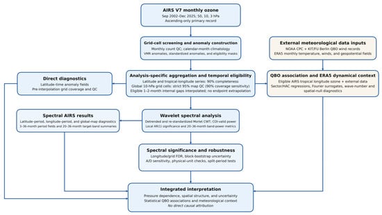
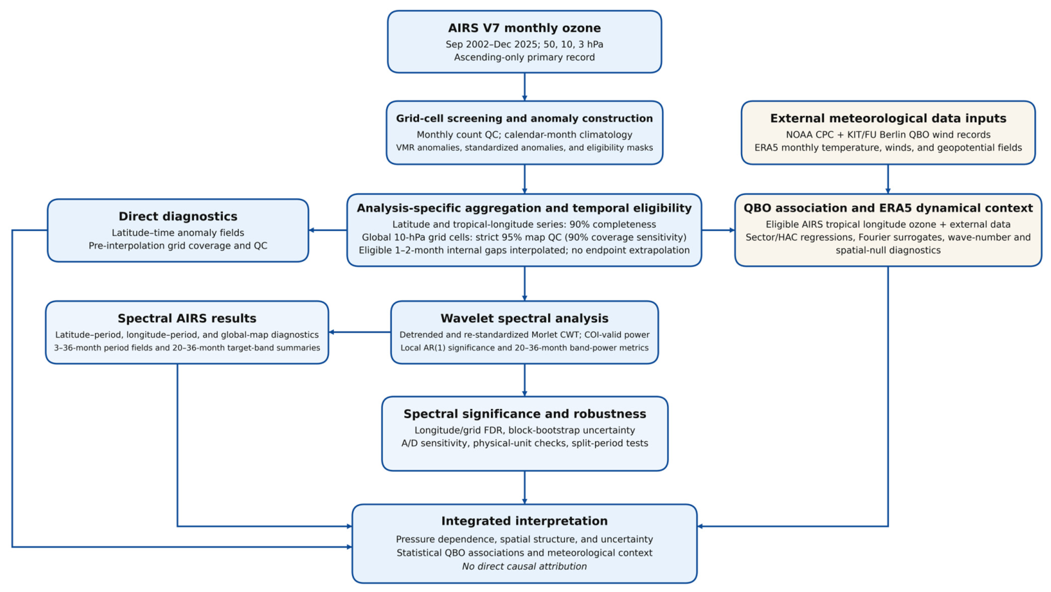
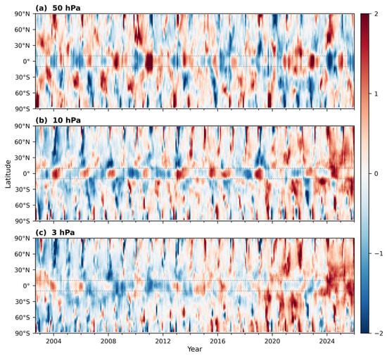
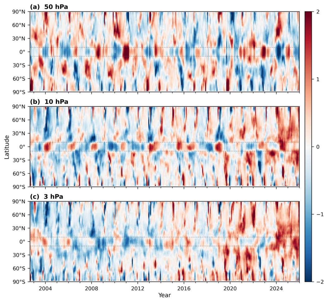
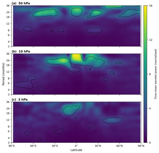
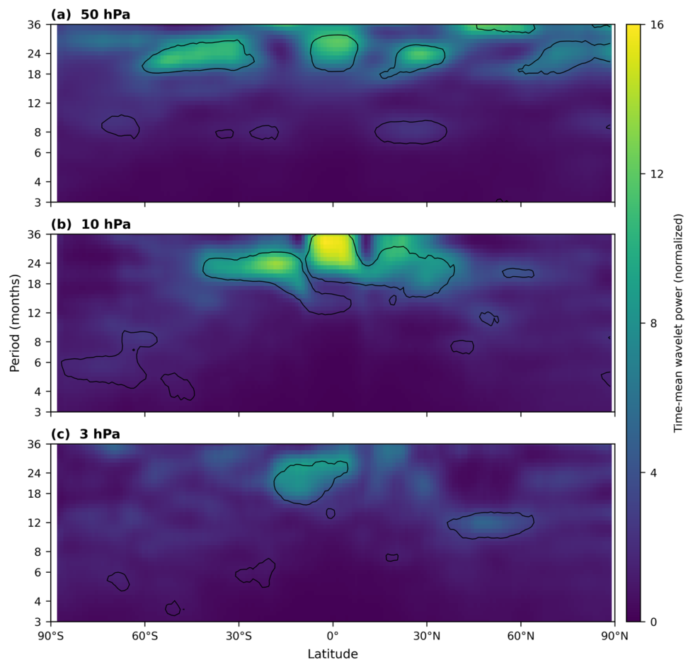
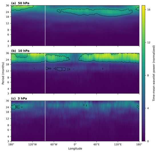
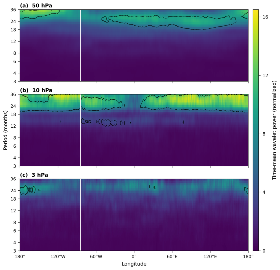
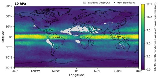
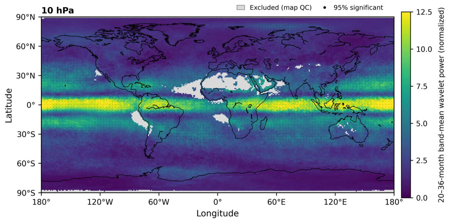
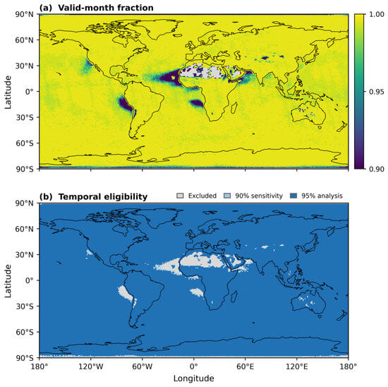
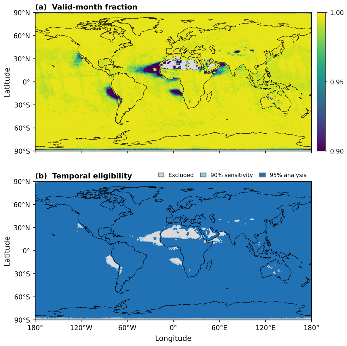
Disclaimer/Publisher’s Note: The statements, opinions and data contained in all publications are solely those of the individual author(s) and contributor(s) and not of MDPI and/or the editor(s). MDPI and/or the editor(s) disclaim responsibility for any injury to people or property resulting from any ideas, methods, instructions or products referred to in the content. |
© 2026 by the authors. Licensee MDPI, Basel, Switzerland. This article is an open access article distributed under the terms and conditions of the Creative Commons Attribution (CC BY) license.