


Highlights
What are the main findings?
- SWIR radiance channels optimized through radiative transfer simulations for their physical sensitivity to lower-tropospheric CH4 enabled near-surface CH4 estimation comparable to that based on retrieval products, indicating that near-surface information is inherently contained in the observed radiance spectrum.
- A stacking ensemble fusing multiple machine learning models with different learning schemes consistently outperformed all individual base learners, with the largest gain when the L2 products and the selected L1B radiances were used together.
What are the implications of the main findings?
- The use of physically selected SWIR radiances enables surface CH4 estimation without dedicated CH4 retrieval products, facilitating application to both current and future satellite missions.
- The proposed framework offers a practical pathway toward observation-based monitoring of large-scale surface CH4 variability; its extension to regions with limited ground-based measurements requires a broader network of training stations.
Abstract
Atmospheric methane is the second-largest contributor to radiative forcing among long-lived greenhouse gases, and characterizing its spatiotemporal distribution is essential for identifying sources and evaluating mitigation policies. Methane emissions are most directly reflected in near-surface concentrations, whereas satellite observations retrieve only the column-averaged methane concentrations. This study presents a physics-informed stacking ensemble framework that estimates surface CH4 directly from TROPOMI SWIR observations. SWIR radiance channels within the 2305–2385 nm band were optimally selected on the basis of their CH4 information content, including the contribution of the lower atmosphere, as quantified by radiative transfer analysis, and these L1B radiances were combined with L2 products and auxiliary variables governing surface concentration formation. Predictions from machine learning models with different learning schemes were fused through a stacking ensemble that exploited their complementary error structures and outperformed all individual base learners against ground-based in situ observations. For years and stations that were not used in training, the ensemble achieved R2 = 0.75 and 0.66, respectively. The selected channels improved estimation performance, and the L1B-only configuration performed comparably without a dedicated CH4 retrieval product, indicating that the observed spectra carry information relevant to surface CH4 before retrieval. The reconstructed global fields reproduced large-scale spatial and seasonal variability with stronger regional contrasts than the input column observations, demonstrating that physically informed channel selection combined with machine learning enables satellite-based surface CH4 estimation.
1. Introduction
Methane (CH4) is the second-largest contributor to radiative forcing among long-lived greenhouse gases after carbon dioxide (CO2), and its atmospheric concentration has continued to increase since the industrial era [1,2]. Although CH4 has a relatively short atmospheric lifetime of approximately 12 years compared to CO2, its 100-year global warming potential (GWP100) is approximately 27–30 times that of CO2 [3]. Consequently, mitigating methane emissions is considered one of the most immediately effective means of curbing warming on decadal timescales, and the 2021 Global Methane Pledge adopted the target of reducing global emissions by 30% by 2030 relative to 2020 levels [4]. However, methane emissions are distributed across numerous source categories with distinct emission mechanisms, including wetlands, ruminant livestock, rice cultivation, fossil fuel production and transport, and waste landfills, making direct global-scale measurement practically infeasible [1]. Therefore, emissions must be inferred indirectly from observable atmospheric state variables. Accordingly, accurately characterizing the spatiotemporal distribution of atmospheric CH4 concentrations is essential for identifying emission sources and evaluating the effectiveness of mitigation policies.
Atmospheric CH4 concentrations are observed or simulated through ground-based and airborne in situ observations, satellite remote sensing, and atmospheric chemical transport models. Ground-based in situ observations directly measure air near the surface with high-precision continuous sampling, thereby providing the most reliable information on absolute concentration levels and their temporal variability [5], and are traceable to internationally agreed standard gas scales, ensuring comparability across stations [6]. However, observation stations are not uniformly distributed across continents and latitude bands, leaving substantial observational gaps in remote regions and oceanic areas, including the tropical and subtropical regions [6,7]. Satellite remote sensing fills these gaps by observing reflected sunlight in the shortwave infrared (SWIR) region, providing good spatial density of observations [7]. For example, there are Greenhouse gases Observing Satellite (GOSAT [8]) and TROPOspheric Monitoring Instrument (TROPOMI [9,10]), both of which provide global coverage as Low Earth Orbit (LEO) satellite, while dedicated methane satellites specialized for point-source detection are also in operation [11]. However, the physical quantity derived from satellite observations is the column-averaged dry-air mole fraction (XCH4), which does not provide information on the vertical distribution of methane. Methane released at the surface first mixes within the atmospheric boundary layer before being diluted upward, so the emission signal remains strongest in surface concentrations; however, the column average does not capture this information. Three-dimensional concentration fields, including the surface layer, can be obtained from chemical transport models (CTMs) [12,13] and from products combining these models with data assimilation or inverse modeling [14,15]. However, their accuracy depends on the prior emission inventory and the representation of transport processes [16,17], and the inventories themselves can deviate substantially from actual emissions for sources with large spatiotemporal variability, such as wetlands and landfills [1,18].
The approach of estimating surface-level value from satellite-derived products has been widely applied to aerosols (e.g., PM10 and PM2.5) or trace gases such as NO2. Such approaches have relied either on column–surface relationships simulated by chemical transport models or on machine learning trained jointly with meteorological and surface auxiliary data [19,20,21]. By contrast, satellite-based studies targeting methane have largely focused on the retrieval accuracy of the column-averaged concentration itself [9,22,23]. The detection mechanism of point-source plumes in hyperspectral imagery [24,25] targets locally enhanced signals relative to background. Even where machine learning approaches have been adopted, their application has mainly focused on bias correction of retrievals or the generation of spatiotemporally continuous column concentration fields [26,27,28,29]. Studies that directly estimate surface CH4 concentrations have only recently appeared [30,31,32], but these generally employ a single-architecture prediction model, restrict inputs to already-retrieved Level-2 (L2) column values and auxiliary variables, and confine training and evaluation to specific regions. The models trained under different inductive assumptions tend to produce different systematic errors. The stacking ensemble, in which predictions from multiple models are combined with weights learned by a meta-learner, can yield more stable predictions than a single model [33,34], and this advantage has been reported for column CH4 concentration retrievals [29]. However, the L2 column values used as input in these studies are products already compressed from radiance to column averages, and thus have already lost information on the vertical distribution. Attempts to exploit satellite-observed radiance directly in machine learning have been reported [35], but the estimation target in that case was the column-averaged concentration, and the problem of estimating surface concentrations, where the effect of emission changes is most directly reflected, has not yet been sufficiently addressed.
In this study, we use a radiative transfer model (RTM) to select optimal SWIR channels based on their CH4 information content and lower-atmospheric sensitivity and combine the observed top-of-atmosphere (TOA) radiances at these channels with satellite-derived L2 products as inputs to machine learning to estimate surface CH4 concentrations. Furthermore, considering that surface CH4 concentrations are jointly governed by the distribution of emission sources and atmospheric transport, we include variables that are physically involved in concentration formation, such as wind speed, surface elevation, aerosol optical depth, land cover, season, and latitude, as inputs, and estimate surface CH4 concentrations by fusing the predictions of machine learning models with different learning schemes through a stacking ensemble. In Section 2, we describe the data used, the procedure for selecting SWIR channels based on radiative transfer simulations, and the training and evaluation methods for the stacking ensemble. Section 3 presents the physical characteristics of the selected channels, the performance of each input configuration and the contribution of individual components, variable contribution analysis, and the results of reconstructing the global surface CH4 distribution.
2. Materials and Methods
The framework of this study consists of two dominant processes: physics-based channel selection and machine learning (ML)-based surface CH4 concentration estimation, with the overall processing flow shown in Figure 1. In the first component, radiative transfer simulations are used to calculate the absorption sensitivity and information content across the SWIR band, from which wavelengths are selected on the basis of their CH4 information content, with additional weighting toward lower-atmospheric (0–5 km) sensitivity and spectral diversity. In the second component, the satellite radiances at the selected wavelengths are combined with auxiliary variables to construct the input features, and a stacking ensemble is trained and evaluated against in situ observations from ground stations. The details are described in the following sections.
Figure 1.
Overall workflow of the proposed framework for estimating surface CH4 concentrations from TROPOMI observations. The workflow consists of four sequential modules: input data collection, physics-informed SWIR channel selection, feature matrix construction with stacking ensemble learning, and evaluation and interpretation.
2.1. Datasets and Preprocessing
TROPOMI is a spectrometer aboard the Sentinel-5 Precursor satellite that provides daily global coverage from a sun-synchronous orbit at approximately 13:30 local solar time [9,10]. In this study, we used Level-1B (L1B) top-of-atmosphere radiance in the SWIR Band 7 and 8 (2305–2385 nm), where CH4 absorption lines are distributed. Because the CH4 absorption signal is contained in these hyperspectral radiances, a subset of channels was selected to construct the spectral input variables for the ML model. The geometric information (solar zenith angle, SZA; viewing zenith angle, VZA; solar azimuth angle, SAA; viewing azimuth angle, VAA) is also required to reflect a residual difference in optical path length and was therefore also included as an input variable. In addition, to combine the information provided by physics-based retrievals with the spectral inputs and to compare their respective contributions, we extracted XCH4, surface elevation, aerosol optical depth, and the zonal and meridional wind speeds from the auxiliary meteorological data from the L2 product of the same observations. These variables represent, respectively, the column-averaged dry-air mole fraction of CH4 (XCH4), optical path length and scattering conditions (surface elevation and aerosol optical depth), and the advection conditions of local emissions (wind speed). In order to obtain only the reliable information from the data, we applied the threshold of the quality flag (qa_value > 0.5) [9,36]. Because the emission environment of CH4 varies with surface type, we used the MODIS (Moderate Resolution Imaging Spectroradiometer) land cover product MCD12C1 (Collection 6.1, 0.05° climate modeling grid, aggregated from the 500 m MCD12Q1 product) [37] as surface characteristic data. From this product, we extracted the International Geosphere-Biosphere Programme (IGBP) land cover classification, bare-ground fraction, and the land–sea mask, which were used to construct input variables representing surface type.
The target values to be estimated by the model, and the reference standard for performance evaluation, are surface CH4 concentrations measured directly at ground stations, obtained from the Global Atmosphere Watch (GAW) station data distributed by the World Data Centre for Greenhouse Gases (WDCGG) [38]. The values at each station are reported by the contributing institutions in accordance with the World Meteorological Organization (WMO) standard scale. For the collocation of satellite and ground-based observations, we included only orbits for which the distance from the station to the nearest pixel was within 50 km. The mean of valid pixels within a 5 × 5 pixels window centered on the corresponding pixel was calculated and used as the satellite input value for the given station and time. The standard deviation of XCH4 computed over the same window was added as a variable representing pixel-scale spatial variability. Given that the TROPOMI pixel size is approximately 5.5–7 km, this window corresponds to an area with a side length of approximately 28–35 km [9]. The ground-based target value was the hourly observation closest to the satellite overpass time within ±1 h. A total of 42 GAW/WDCGG stations on six continents and in Oceania (Figure S1 and Table S1) contributed 4657 collocated samples over 2018–2024.
For the collocation, the IGBP class of the 0.05° grid cell containing the center pixel of the 5 × 5 TROPOMI window was used. The bare-ground fraction was computed as the fraction of 0.05° cells classified as barren or open shrubland within the 5 × 5 block of cells (0.25° × 0.25°) centered on this cell, and the land–sea mask was derived from the IGBP water class. These variables describe the surface type and emission environment (e.g., wetland, cropland, or barren land) rather than the seasonal state of the surface; the seasonal variability of the inputs is carried by the time-varying satellite variables and the seasonal terms (sin(DOY) and cos(DOY), where DOY is the day of year).
The land cover variables were used to represent the surface characteristics related to both the observed radiance and the CH4 emission environment. The radiative effect of the surface at the time and wavelength of each observation is reflected jointly in several satellite inputs, including the L1B radiances, the observation geometry, the aerosol optical depth, and the L2 XCH4, whose retrieval accounts for the surface albedo [10].
2.2. Spectral Channel Selection Based on Radiative Transfer Model
The spectral channels to be used as inputs for machine learning in the SWIR Band 7/8 range were selected based on simulations of the physical properties of each wavelength using an RTM. The absorption characteristics of individual trace gases and the sensitivity of the radiance at each wavelength to changes in CH4 at different altitudes were simulated, and the information content of wavelength combinations was quantified using the degrees of freedom for signal (DFS). Finally, the channel combination was determined using a selection algorithm that jointly considers information content and sensitivity.
2.2.1. Radiative Transfer Simulation and Spectral Absorption Characteristics
The spectral information required for channel selection was calculated using Unified Linearized Vector Radiative Transfer Model (UNL-VRTM) [39], a vectorized radiative transfer model that is based on the Vectorized Linearized Discrete Ordinate Radiative Transfer (VLIDORT; [40,41]). From the RTM, we simulate each molecular effect on a line-by-line while simultaneously deriving analytical Jacobians with respect to the CH4 profile, both the wavelength-dependent absorption characteristics of trace gases within the band and the altitude-resolved CH4 sensitivity at each wavelength can be obtained. The simulation was performed from 2305 to 2385 nm, corresponding to the spectral range observed by TROPOMI SWIR Bands 7 and 8, using the TROPOMI instrument spectral response function with a full width at half maximum (FWHM) of approximately 0.25 nm, at a spectral sampling of 0.1 nm (801 wavelengths). The reference simulation for the channel selection assumed a solar zenith angle of 15°, a near-nadir viewing geometry, and a surface albedo of 0.30; the dependence of the selection on the SZA and surface albedo is examined in Section 3.1. The atmosphere was represented by 48 vertical layers from the surface to the top of the atmosphere (TOA), following the vertical profile of the US Standard Atmosphere [42], and included CH4 together with other absorbing gases such as H2O, CO2, O3, N2O, and CO. The spectral parameters for the molecular absorption lines were taken from the High-resolution Transmission Molecular Absorption (HITRAN) database [43], with water vapor continuum also taken into account. The surface was assumed to behave as a Lambertian reflector, and scattering was limited to Rayleigh scattering under clear-sky conditions. Aerosols were not included in the simulation. Instead, their effect was accounted for indirectly at the ML input stage by including TROPOMI L2 aerosol optical depth as an input variable.
Because the RTM computes layer-by-layer absorption optical depth (τ) separately for each gas species, the spectral contributions of the target gas (CH4) and interfering gases can be evaluated independently. The simulation results show that CH4 and H2O are the only gases exhibiting significant absorption in the 2305–2385 nm band (Figure 2a). CO reaches only about 1/60 of the CH4 peak value while the other absorbing gases exhibit even weaker signals. CO2 in particular is negligible, giving this band the spectroscopic advantage of gathering CH4 information with minimal interference from CO2. Accordingly, the only major interfering absorber for CH4 in this band is H2O, and this tendency is pronounced over a broad, contiguous spectral range (Figure 2b). This means that channel selection in this band cannot be determined solely by the strength of CH4 absorption but must also account for the relative contribution of H2O.
Figure 2.
(a) RTM-simulated column optical depths of CH4 (blue), H2O (red), CO (green), and other trace gases combined (gray) in SWIR spectral range (2305–2385 nm). (b) Fractional contribution of each gas to the total optical depth at each wavelength.
The layer-by-layer optical depth of CH4 is relatively uniform across altitude, whereas H2O absorption is concentrated in the boundary layer (0–2 km) and the lower free troposphere (2–5 km). The layer- and wavelength-resolved optical depth distributions of the interferent gases are shown in Figure S2. In other words, the altitude range where the surface CH4 signal resides coincides with the altitude range where H2O interference is strongest. Nevertheless, the channel selection in this study does not exclude these H2O-dominant wavelengths in advance. In optimal estimation (OE) approach, an interfering absorber that is not jointly retrieved propagates directly into retrieval error. However, in a data-driven model that receives multiple channels simultaneously as input, channels with strong H2O absorption can also provide information that constrains the water vapor state. Instead, the channel selection procedure (see Section 2.2.3), which is built around ΔDFS based on the CH4 Jacobian, naturally favors wavelengths with strong CH4 absorption, even without an explicit constraint on H2O.
The optical depth indicates only the amount of absorbing gas present but does not indicate how strongly the radiance at a given wavelength responds to a change in CH4 at a specific altitude. The quantity describing this response is the Jacobian. The RTM computes the Jacobian for each atmospheric layer and wavelength. This is a physical quantity representing the change in TOA radiance I(λ) resulting from a unit change in the CH4 volume mixing ratio (VMR) of layer i. Then, it is converted into a dimensionless relative sensitivity by applying the standard normalization via following equation.
where is the dimensionless normalized Jacobian for layer i and wavelength λ, is the partial derivative of the TOA radiance with respect to the CH4 volume mixing ratio of layer i, VMR(i) is the CH4 volume mixing ratio of layer i, I(λ) is the TOA radiance at wavelength λ, and i = 1, …, 48 denotes the atmospheric layer number from the surface to the top of the atmosphere. corresponds to the relative change (%) in TOA radiance at wavelength λ resulting from a 1% change in the CH4 mixing ratio of layer i, thereby allowing sensitivities at all layers and wavelengths to be compared on a common scale (Figure 3).
Figure 3.
Vertical distribution of the normalized CH4 Jacobian in the TROPOMI SWIR band (2305–2385 nm). (a) Wavelength–altitude distribution of the normalized Jacobian. (b) Fractional contribution of the boundary layer (BL, 0–2 km), lower free troposphere (LFT, 2–5 km), upper free troposphere (UFT, 5–15 km), and stratosphere (STRAT, 15–50 km) to the normalized Jacobian at each wavelength.
To quantify the sensitivity of the altitude contribution from the normalized Jacobian, the atmosphere is classified into four layers: the boundary layer (BL, 0–2 km), the lower free troposphere (LFT, 2–5 km), the upper free troposphere (UFT, 5–15 km), and the stratosphere (STRAT, 15–50 km). The contribution fraction of each layer is defined as the ratio of the sum of the absolute values of for the layers within the region. The BL top was fixed at 2 km, which is comparable to the typical daytime convective boundary-layer depth over land [44,45]; this simplifying assumption is used only to diagnose the BL contribution, whereas the selection score of Equation (6) uses the 0–5 km fraction, which does not depend on this boundary. The actual BL height varies with atmospheric stability, season, and surface type, but this fixed boundary provides a consistent reference for wavelength comparison.
where BLfrac(λ) is the fraction of the total Jacobian at wavelength λ attributable to the boundary layer, with the numerator given by the sum of over layers i belonging to the BL region and the denominator given by the sum over all layers. The contribution fractions for LFT, UFT, and STRAT are defined in the same way, and the four fractions sum to 1.0.
The BL contribution fraction depends on the absorption strength at each wavelength: it decreases as the CH4 column optical depth τ increases, whereas the absolute BL sensitivity (the sum of the absolute normalized Jacobian over the BL layers) increases with τ, because the magnitude of the Jacobian scales with the absorption strength. This wavelength dependence is consistent with the pressure dependence of the absorption line shape [46,47] rather than with the attenuation along the light path, and it is preserved under different atmospheric profiles and instrument spectral response functions (Figure S3). This trade-off between relative and absolute sensitivity allows altitude-dependent information to be partially separated through wavelength selection, but the BL contributes only about 10% of the sensitivity of the selected channels (Section 3.1).
2.2.2. Analysis of Degree of Freedom for Signal
To select the optimal channels, it is necessary to consider not only the altitude-resolved sensitivity of individual wavelengths but also the amount of independent information provided by a given combination of wavelengths when used simultaneously.
This information content was quantified using the DFS, which represents the number of independent pieces of information that a selected wavelength combination provides regarding the atmospheric state vector [48]. To calculate the DFS, the prior covariance matrix Sₐ of the CH4 vertical profile is constructed as follows. Because the normalized Jacobian already incorporates the VMR scaling, Sa is likewise defined in this same normalized space.
where Sa(i, j) is the prior covariance component between layers i and j, and σrel is the relative prior uncertainty of each layer, assumed to be 10%. Here zi and zj are the center altitudes of layers i and j, respectively, and Lcorr = 5.0 km is the vertical correlation length. The exponential correlation structure is a covariance model reflecting the fact that CH4 in adjacent altitude layers is mutually correlated, and Lcorr = 5.0 km, as adopted in this study, represents a characteristic scale of vertical mixing in the free troposphere. The measurement error covariance Se was set as Se = diag(1/SNR2), assuming a signal-to-noise ratio (SNR) of 150. Because Se, like , is defined in the normalized space, the measurement error is likewise expressed as a relative error. These parameter values were used as fixed assumptions for the information content-based channel selection analysis.
From the normalized Jacobian matrix for a selected wavelength combination, the averaging kernel matrix A is constructed as follows:
where is the normalized Jacobian matrix defined in Equation (1), Sa is the prior covariance matrix, and Se is the measurement error covariance matrix. The diagonal element A(i, i) represents the degree to which CH4 in layer i is constrained by the observation, and the DFS is therefore expressed as follows:
DFS = tr(A)
The altitude-resolved DFS (Zone DFS) quantifies the information content associated with a given altitude zone and is defined as the sum of A(i, i) over the layers i within that zone. The Zone DFS values over the four zones sum to the Total DFS.
2.2.3. Machine Learning-Diverse Channel Selection
Based on the DFS as described above, the channel subset is selected as follows. We restrict the ML input to an optimal subset in terms of CH4 information content rather than using the full set of wavelengths. If training data are limited, a high input dimensionality may lead to poorer generalization performance. This effect is known as the curse of dimensionality [49]. A similar need to reduce the number of input channels in advance has been reported for hyperspectral radiances used as neural network inputs [50]. The same problem is well established in OE retrievals. When channels are highly correlated, additional channels add little independent information and mainly propagate measurement noise into the inverse solution. An information-based selection of an optimal channel subset therefore becomes essential [51]. Further, the SWIR region carries the absorption signatures of interfering species such as H2O and CO in addition to CH4 absorption information [9]. Wavelengths dominated by these non-target absorbers introduce variability unrelated to surface CH4. Including them without screening can degrade model performance [52].
A common approach is information-content-based iterative channel selection. This method initializes the subset as empty and adds the channel with the largest DFS increment at each step [52,53,54,55]. However, sequential selection based on DFS maximization tends to crowd the selected channels into the spectral region of strongest CH4 absorption. Such crowding is acceptable in OE-based retrieval, but for ML training the crowded channels are expected to provide largely redundant inputs. Estimating surface concentrations from the column average requires the model to exploit radiance differences among wavelengths with different BL contribution fractions. Consequently, we sought a diverse set of wavelengths spanning a broad spectral range.
To address these issues, we augment the conventional sequential DFS selection with two correction terms that account for lower-atmosphere sensitivity and spectral diversity. The selection is initialized with an empty set and continues until N channels are obtained. At each step, candidate wavelengths are restricted to those separated from the previously selected channels by at least a minimum channel spacing of 0.5 nm. This value corresponds to approximately twice the spectral resolution of the TROPOMI SWIR (FWHM of about 0.25 nm) [9,10], and it prevents the redundant selection of channels within the spectral resolution. Among these candidates, the wavelength added to the selected set is the one with the maximum selection score, which is defined as follows:
where Score(λc) is the selection score of a candidate wavelength λc, and ΔDFS(λc) is the DFS increment obtained when the candidate wavelength λc is added; it is the same information content criterion used in conventional sequential selection [52,53]. Lowerfrac(λc) is the contribution fraction of the lower atmosphere (0–5 km), obtained by summing the contribution fractions of the BL and LFT, each defined as in Equation (2). is the mean distance between the candidate wavelength λc and each wavelength in the already-selected channel set S, and Δλ is the total width of the spectral range considered for channel selection. α and β are dimensionless weighting coefficients that control the strength of the preference for lower-atmosphere sensitivity and spectral diversity. The lower-atmosphere sensitivity term (α) prevents the exclusion of wavelengths sensitive to the lower atmosphere, which make only a small contribution to the total Jacobian but are essential for surface concentration estimation. The spectral distance term (β) prevents the local crowding of channels and promotes the distribution across the full spectrum of both the wavelengths relatively sensitive to the boundary layer (2340–2362 nm) and the reference wavelengths mainly sensitive to the upper atmosphere (2305–2320 nm, 2370–2385 nm). In this study, α = 3.0 and β = 0.1 were adopted to provide moderate preference for lower-atmosphere sensitivity and spectral diversity. The value α = 3.0 was set so that, when multiplied by the Jacobian-based lower-atmosphere contribution fraction Lowerfrac (BL + LFT), the lower-atmosphere sensitivity correction term of the score (1 + α · Lowerfrac(λc)) falls within a range of approximately 1.6–2.2. This level gives an approximately twofold preference to lower-atmosphere-sensitive wavelengths among candidates with comparable DFS increments, while keeping the DFS increment itself as the dominant criterion. The value β = 0.1 was chosen to apply a diversity correction of at most 10% to the score, so that the information content criterion remains the primary selection criterion. The selected channel set therefore contains channels with differing BL contribution fractions. When these channels are provided together as input, the ML model estimates surface CH4 from the signal differences among them, while accounting for the contribution of the upper atmosphere.
2.3. Configuration, Training, and Evaluation of the Machine Learning Model
The surface CH4 retrieval model was designed as a two-stage ensemble that combines the predictions of multiple regression models. In the first stage, five base learners were selected to represent four distinct learning paradigms with different function approximation characteristics. Two boosting-based models, LightGBM and XGBoost, were adopted [56,57], while Random Forest was employed as the bagging-based model [58]. LightGBM and XGBoost sequentially construct shallow decision trees by fitting the residuals from the preceding iteration, thereby capturing nonlinear relationships and interactions among predictor variables. However, because LightGBM employs a leaf-wise tree growth strategy whereas XGBoost uses a depth-wise strategy, the two algorithms typically converge to different partitioning structures even when trained on the same dataset. Random Forest, in contrast, averages predictions from a large number of independently trained decision trees built on bootstrap samples, providing robust predictions that are less sensitive to noise. Despite these differences, all three tree-based models rely on axis-aligned recursive partitioning, resulting in piecewise-constant prediction surfaces and limited extrapolation capability beyond the range of the training data.
To complement these characteristics, two models that directly approximate continuous nonlinear functions were incorporated. Support Vector Regression (SVR) with a radial basis function (RBF) kernel [59,60] learns smooth nonlinear mappings using the ε-insensitive loss function, making the model relatively insensitive to local residual fluctuations. An artificial neural network (ANN) consisting of a single-hidden-layer multilayer perceptron (MLP) was also employed. Owing to its universal approximation property [61], the ANN is capable of learning nonlinear functions that combine information from all input variables [62].
For continuously varying inputs such as the 20 highly correlated SWIR channels, the SVR and ANN tend to produce prediction errors that differ systematically from those of the tree-based models. This diversity in error characteristics among the five base learners is what the second-stage ensemble exploits. Because both SVR and ANN are sensitive to the scale of the input variables, standardized predictors were used for these two models.
The stacking ensemble consists of a two-stage architecture comprising the five base learners in the first stage and a Ridge regression [63] meta-learner in the second stage. Hereafter, this ensemble is referred to as the Ridge Ensemble. The ensemble prediction is given by
where ŷ is the surface CH4 concentration estimated by the ensemble, x is the input variable vector, fk(x) is the prediction of the k-th base learner, wk is the Ridge weight assigned to that model, b is the intercept, and k = 1, …, 5 is the base learner index. The out-of-fold (OOF) predictions of the five base learners are used as meta-variables. The meta-variables are standardized to zero mean and unit variance and then input to the Ridge regression [62]. The regularization strength of the Ridge regression was not fixed but selected through cross-validation within the training data of each fold.
The model inputs were designed in three configurations, namely L2, L1B, and a combined L2+L1B configuration, to compare the contribution of each information source. The three configurations include the same set of 14 common variables. The common variables consist of three temporal variables (sin(DOY), cos(DOY), and year_fraction), four observation geometries (SZA, VZA, SAA, and VAA), three MODIS surface variables (IGBP land cover classification, bare-ground fraction, land–sea mask), and four latitude harmonic functions (sin(lat), cos(lat), sin(2lat), and cos(2lat)). Among the temporal variables, sin(DOY) and cos(DOY) represent the seasonal cycle, whereas year_fraction is a continuous time index that increases monotonically over the study period and therefore represents the long-term trend in atmospheric CH4. To these, the L2 configuration adds six TROPOMI L2 variables (the window mean and standard deviation of XCH4, surface elevation, aerosol optical depth, and zonal and meridional wind speeds), giving 20 variables in total. The L1B configuration adds the SWIR radiances of the 20 channels selected in Section 2.2, giving 34 variables, and the L2+L1B configuration adds both sets. Because the three configurations include the same common variables, the performance differences among the configurations correspond to the distinct contributions added by the L2 variables and the L1B variables, respectively. In particular, the L1B configuration was designed to evaluate whether the selected L1B spectral radiances provide sufficient predictive information for estimating surface CH4 when combined with the common spatiotemporal, geometric, and surface variables, without relying on the L2 product.
To evaluate the temporal generalization capability, we applied a group-wise cross-validation using the observation year as the grouping variable (leave-one-year-out cross-validation, LOYO CV). All collocation samples belonging to a given year were held out as the validation set, and the model was trained using only samples from the remaining years. This process was repeated so that each year served as the validation set once. Because the data of the validation year were never used in the training of the corresponding fold, the generalization performance of the model can be evaluated for atmospheric states in periods it had not been trained on. The cross-validation was performed on the 2018–2024 collocation data, and all three configurations used the same fold partitioning to ensure comparability among configurations. The base learners were fitted on the training years of each fold, and the Ridge meta-learner was fitted on the out-of-fold base-learner predictions for those training years; the models were then applied to the held-out year, and the resulting predictions were used to compute the overall and fold-wise performance. The estimation performance of the model was evaluated using the coefficient of determination (R2), the root-mean-square error (RMSE), the mean absolute error (MAE), and the mean bias, defined as the estimate minus the observation.
The hyperparameters of the five base learners were optimized using the Tree-structured Parzen Estimator (TPE) algorithm in Optuna [64]. The optimization was performed independently for each of the three input configurations, with a single hyperparameter search conducted over the entire cross-validation procedure for each configuration. The objective of the search was the RMSE of the LOYO CV described above, with 80 trials for LightGBM and XGBoost, 60 for ANN, and 50 for Random Forest and SVR. The performance comparison among configurations is therefore a comparison of the performance that each input configuration attains at its own optimal hyperparameters. Forcing identical hyperparameters would place the L2+L1B configuration, which has twice as many input variables as the L2 configuration, at a structural disadvantage. Ridge was selected as the meta-learner because it allows negative weights, which can cancel out errors common to the base learners, and because its regularization enables the stable combination of highly correlated OOF predictions while keeping the weights easy to interpret.
Because the hyperparameters were tuned on the same LOYO splits used for evaluation, the LOYO scores may be optimistically biased. We therefore also performed a nested CV for each of the three input configurations, in which, for each outer LOYO fold, the hyperparameters of the five base learners (15 Optuna trials per model) and the Ridge meta-learner were determined using only the training years through an inner LOYO CV, and the held-out year was used only for evaluation (Table S2).
To assess spatial generalization, we additionally performed a 42-fold leave-one-station-out cross-validation (LOSO CV), in which all observations of each station were held out in turn and excluded from model fitting, following the station-based evaluation of satellite-derived surface PM2.5 and NO2 [19,21]. The hyperparameters optimized on the LOYO splits were used without re-tuning, so that the LOYO and LOSO scores refer to the same model configuration.
Feature contributions were interpreted using SHAP (SHapley Additive exPlanations) [65]. SHAP attributes the prediction of an individual sample to the contributions of each input feature, such that the prediction can be expressed as the sum of the baseline prediction and the feature contributions. The relationship is expressed as follows:
where f(x) is the estimate of the stacking ensemble for the input variable vector x, equivalent to ŷ in Equation (7). φ0 is the mean of the estimates over all samples, which serves as the reference value for the contribution decomposition. φj is the contribution of the j-th variable to the deviation from this reference value, that is, the SHAP value, and M is the number of variables. The SHAP values for the entire stacking pipeline, comprising the five base learners and the Ridge meta-learner, were computed using a model-agnostic kernel-based approximation. This approach reflects the contribution from the original variable space to the final ensemble estimate, allowing the direction and magnitude of variable contributions to be analyzed at the level of individual samples.
3. Results
3.1. Information Content and Spectral Distribution of the Selected Channels
To determine the number of input channels (N), we calculated the DFS while increasing the number of channels from 1 to 100. At (N = 20), the Total DFS and BL DFS reached 1.068 and 0.1018, respectively, after which further increases became markedly smaller (Table S3). The information efficiency (DFS/(N)) decreased sharply from 19.7% at (N = 5) to 5.3% at (N = 20) and 1.1% at (N = 100). In addition, the fraction of the Total DFS attributed to the 0–5 km layer remained nearly unchanged, increasing only from 27.0% at (N = 20) to 28.7% at (N = 100). This indicates that most of the information provided by the additional channels is associated with the upper atmosphere. Since increasing the number of selected channels inevitably includes wavelengths with relatively low CH4 information content, we adopted (N = 20) in this study.
Without a minimum channel spacing, sequential selection based solely on ΔDFS places 13 of the 20 channels within the narrow interval near 2365–2375 nm, where CH4 absorption is strongest. This occurs because a criterion based solely on ΔDFS repeatedly selects wavelengths with strong absorption and large Jacobian amplitudes. The minimum channel spacing of 0.5 nm reduces this crowding, and with the two additional terms of Equation (6), the ML-Diverse algorithm distributes the 20 channels over the entire band, with a spectral standard deviation of 21.2 nm. Because ΔDFS remained the primary optimization criterion and the two additional terms served only as secondary constraints, the increased spectral diversity was achieved without replacing the information-content criterion. The BL contribution fractions of the 20 selected channels range from 7.1% to 12.4%, with a mean of 10.1% (Figure 4).
Figure 4.
The SWIR channels selected on the basis of radiative transfer simulations. The gray line shows the simulated TOA normalized radiance spectrum, and circles mark the channels selected by the ML-Diverse algorithm, colored according to the boundary-layer (0–2 km) fraction of the Jacobian at each channel.
We tested whether the selection results depend on particular atmospheric conditions and whether the selected channels indeed respond to changes in lower-atmospheric CH4. To evaluate the dependence on observation conditions, channel selection was performed independently for 16 conditions combining four SZA values (15°, 30°, 45°, and 60°) with four surface albedo values (0.05, 0.10, 0.20, and 0.30). Because albedo cancels in the normalized Jacobian under the Lambertian reflection assumption, the albedo axis serves as a null test confirming that this cancellation also holds numerically. The substantive variation in the selection therefore arises along the SZA axis. Seventeen of the 20 channels were selected in common across all 16 conditions, and the pairwise overlap between conditions averaged 18.7 channels (93.5%). Because this mean was computed over all pairs, including those differing only in albedo, it should be interpreted as an upper bound on the stability with respect to SZA. The three remaining channels (2318.1, 2318.6, and 2355.9 nm) were mostly replaced by adjacent wavelengths, reflecting the change in optical path length with SZA in the fine structure of the Jacobian spectrum. This stability arises because the shape of the Jacobian spectrum does not vary substantially with observation conditions (Figure S4).
A downstream comparison with simpler selection strategies (sequential DFS maximization and uniform spacing of 20 channels within the same 2305–2385 nm band), using identical models and the LOYO CV, showed that every 20-channel set performed better than the full band (ensemble R2 = 0.752–0.753 vs. 0.748; Table S4), whereas the differences among the 20-channel sets were small. Reducing the input to a compact set of channels therefore does not degrade the performance, and the prediction skill gained from the L1B radiances arises from the information contained in this band rather than from a specific channel combination. The practical role of the information-content analysis is to determine, without training data, a small number of channels and to provide channels with physically interpretable vertical sensitivity, reducing the number of radiance inputs without loss of performance.
3.2. Model Performance by Input Configuration and the Contribution of Radiance
The cross-validation performance of the three input configurations (L2, L1B, and L2+L1B) is summarized in Table 1. The R2 was highest for the L2+L1B configuration, which uses the selected radiance channels within SWIR together with the retrieved L2 product, at 0.753 (RMSE = 33.98 ppb), followed by the L2 configuration at 0.742 (RMSE = 34.78 ppb) and the L1B configuration at 0.725 (RMSE = 35.91 ppb). Under the nested CV (Section 2.3), the corresponding R2 values were 0.737, 0.723, and 0.698, respectively, and the ranking of the configurations was therefore unchanged (Table 1 and Table S2). Under the LOSO CV (Section 2.3), the Ridge Ensemble of the L2+L1B configuration retained R2 = 0.656 (RMSE = 40.1 ppb) at stations that were not used in training and remained the best-performing model (Table S5 and Figure S5). Because the three configurations were evaluated on the same collocation samples with the same fold partitioning, the comparisons among configurations below are paired comparisons on identical samples. The L2 and L2+L1B configurations share both the common variables and the L2-specific variables, differing only in whether the radiances of selected channels are included. The performance difference between the two configurations therefore corresponds to the additional information provided by these channels. Adding these channels improved the performance of the Ridge Ensemble by 0.011 in R2, 0.80 ppb in RMSE, and 0.63 ppb in MAE. Even without any L2 retrieval product, the L1B configuration attains a comparable level of performance, with an R2 of 0.725 and an RMSE of 35.91 ppb, only 0.017 lower in R2 and 1.13 ppb higher in RMSE than the L2 configuration. This shows that surface CH4 can be estimated from the spectral radiances and the common variables alone, without any L2 retrieval product.
Table 1.
Cross-validation performance metrics of the Ridge Stacking Ensemble model evaluated across different input configurations (L2, L1B, and combined L2+L1B). LOYO R2, bias, MAE, and RMSE are from the LOYO CV; the nested CV R2 is from the nested CV, in which the hyperparameters and the Ridge meta-learner were determined using only the training years of each outer fold (Section 2.3; Table S2).
Station-level validation metrics were computed for each of the 42 GAW/WDCGG stations (Table S1). Of the 35 stations with at least 10 collocated samples, 32 (91%) showed positive R2. Relative to the L2 configuration, adding the L1B radiances reduced the station RMSE at 18 of the 30 Northern Hemisphere mid- and high-latitude stations, which provide 78% of the samples, whereas the RMSE computed over all tropical and Southern Hemisphere samples changed by less than 0.5 ppb (Figure S6). The improvement in Table 1 is therefore concentrated in the well-sampled domains defined in Section 4.
3.3. Individual Model Performance and the Effect of the Stacking Ensemble
Stacking consistently improved the predictive performance over all individual base learners. For the L2+L1B configuration, the Ridge Ensemble achieved the highest predictive performance with an R2 of 0.753, exceeding the best-performing individual model, Random Forest (R2 = 0.727) (Table 2 and Figure 5). Corresponding comparisons for the L1B and L2 configurations are presented in Tables S6 and S7, respectively. The predictive performances of the five base learners were relatively homogeneous for the L2+L1B configuration, with R2 values ranging from 0.702 to 0.727. The difference between the best- and worst-performing models was only 0.025, approximately half that of the L1B configuration (0.049; 0.660–0.709). This suggests that when both L2 and L1B information are available, the predictive performance becomes less dependent on the choice of model architecture. Despite the relatively small differences among the individual models, the Ridge Ensemble further improved prediction accuracy, increasing R2 by 0.026 and reducing RMSE by 1.75 ppb relative to the best-performing base learner. This advantage was maintained under the nested CV, in which the Ridge Ensemble (R2 = 0.737) exceeded the best-performing base learner (XGBoost, R2 = 0.704) by 0.033 (Table S2). In comparison, under the LOYO CV, the ensemble improved R2 by 0.016 for both the L2 and L1B configurations, indicating that the benefit of stacking was greatest when both information sources were used together.
Table 2.
Predictive performance comparison between individual base learners and the Ridge Stacking Ensemble model under the full L2+L1B input configuration (LOYO CV).
Figure 5.
Density plots between observed and predicted surface CH4 concentrations (ppb) for the five individual base learners (LightGBM, XGBoost, Random Forest, SVR, and ANN) and the Ridge Stacking Ensemble evaluated under the L2+L1B input configuration (LOYO CV).
The performance gain from stacking is associated with the predictive diversity among the base learners. The Pearson correlation coefficients between the out-of-fold (OOF) predictions of the five models ranged from 0.85 to 0.95. Correlations among the three tree-based models (LightGBM, XGBoost, and Random Forest) were consistently higher than those between the tree-based models and either SVR or ANN. The lower correlations between different model families indicate that they capture different aspects of the input–output relationship and therefore produce distinct error structures, allowing the ensemble to partially cancel individual model errors through linear combination. The differences in error structure are also reflected in the performance metrics. Although SVR achieved an R2 of 0.722, comparable to that of XGBoost, it produced the lowest MAE among the five base learners (21.90 ppb) while exhibiting the highest RMSE-to-MAE ratio (1.65). This combination indicates that SVR produced relatively small errors for most samples but comparatively large errors for a limited number of cases. Such an error distribution is consistent with the ε-insensitive loss function, which does not penalize residuals within the ε margin. SVR showed the highest RMSE-to-MAE ratio among the base learners in all three input configurations.
The mean bias of the ensemble is smaller than that of the individual models. Four of the five base learners show a negative bias with an absolute value of 0.97–2.93 ppb, whereas the Ridge Ensemble bias is within an absolute value of 0.13 ppb for all three configurations (Table 1 and Table 2). In this architecture, however, the systematic bias of the individual models is removed in the standardization of the meta-variables and the mean level of the ensemble is determined by the intercept, so this value cannot be interpreted as evidence of error cancellation. The gain of the ensemble appears in the reduction of RMSE and MAE. The predictive capability of the models is limited for cases in which the surface CH4 concentration is particularly high. The RMSE for the upper concentration range of the training samples (>2020 ppb) is 54.95 ppb, substantially exceeding the 33.98 ppb of the full sample. In the scatter plots as well, the predictions of all six models are distributed over a narrower range than the observations, and even for samples with observations above 2200 ppb the predictions do not exceed approximately 2100 ppb (Figure 5). This limitation stems from the scarcity of high-concentration samples in the training data. A model trained mainly on the densely sampled concentration range exhibits a regression-to-the-mean tendency, pulling extreme values outside that range toward the sample mean. That the same tendency is common to all six models suggests that this limitation arises from the concentration distribution of the training samples rather than from the architecture of any particular model.
3.4. Feature Contribution Analysis
To quantify the contribution of each input variable to the surface CH4 estimates, we applied SHAP to the Ridge Ensemble. The direction and magnitude of the feature contributions for the L2+L1B configuration are shown in Figure 6. Among the feature categories, spatial variables contributed the largest fraction of the total SHAP importance (36.8%), followed by temporal (24.3%), radiance (16.9%), and L2 XCH4 variables (8.3%). Geometry and meteorology each accounted for 4.2%, while topography, aerosol, and land surface contributed 2.5%, 1.8%, and 1.0%, respectively.
Figure 6.
SHAP feature contribution analysis for the Ridge Stacking Ensemble model under the L2+L1B configuration: (a) mean absolute SHAP values for the 20 most important features; (b) relative contribution by feature category; and (c) beeswarm plot showing the direction and distribution of SHAP values across all samples.
Collectively, the SWIR radiance variables (16.9%) contributed about twice the share of the XCH4 variables (8.3%) and a share comparable to that of all six TROPOMI L2 variables combined (16.8%). Feature importance was concentrated in a small number of variables. The latitude harmonic variables collectively contributed the largest share, with sin_lat alone accounting for 25.4% of the total SHAP importance across all variables. Together with year_fraction (17.6%), these two variables explained 43.0% of the total importance. Although the contribution of each individual SWIR channel was relatively smaller than above, five selected SWIR channels were ranked among the 20 most important variables (especially, 2371.20 and 2307.50 nm).
The SHAP beeswarm plot of sin_lat, the most influential feature, shows a clear separation into two groups. Samples from the Southern Hemisphere, corresponding to the lowest sin_lat values, are tightly clustered between −80 and −60 ppb, whereas those from the Northern Hemisphere are continuously distributed between 0 and +50 ppb. This pattern indicates that the model primarily distinguishes the difference in background CH4 concentrations between the two hemispheres rather than representing latitude as a smooth gradient. Consistent with this interpretation, cos_lat, which increases toward lower latitudes, exhibits negative SHAP contributions. This bimodal structure also agrees with the observed distribution of surface CH4 concentrations (Figure 5). In contrast, the SHAP values of year_fraction increase monotonically with increasing feature values, indicating that the model captures the long-term increase in surface CH4 through the temporal variable. Among the selected SWIR channels, 2371.20 nm (3.3 ppb) and 2307.50 nm (3.1 ppb) showed the largest individual contributions. The two channels represent contrasting absorption conditions within the absorption band. At 2307.50 nm, near the short-wavelength end of the band, CH4 absorption is moderate (τ = 0.28) and H2O absorption is negligible (τ < 0.01), whereas 2371.20 nm lies in the strongly absorbing part of the band (τ = 0.42) but is also strongly affected by H2O (τ = 0.56), so that its radiance also carries information on the water vapor state (Section 2.2.1). Their SHAP patterns exhibit opposite trends. At 2371.20 nm, high radiance values are associated with negative SHAP values and low radiance values with positive SHAP values, consistent with stronger absorption corresponding to higher predicted CH4 concentrations, whereas the 2307.50 nm channel exhibits the opposite relationship. Because the absolute radiance varies mainly with surface reflectance and observation geometry, these opposite signs are consistent with the model using the contrast between channels with different absorption characteristics rather than the radiance of a single channel.
3.5. Spatial and Seasonal Characteristics of the Reconstructed Surface CH4 Fields
The trained machine-learning framework was applied to the global TROPOMI L2/L1B observations for 2020 to reconstruct seasonal surface CH4 concentration fields on a 0.5° grid (Figure 7). To assess whether the reconstructed fields capture the large-scale spatial and seasonal variability of surface CH4, they were compared with three model-based surface CH4 concentration products (CarbonTracker-CH4 [15], CAMS inversion [66], and CAMS-EGG4 [14]), together with the input TROPOMI L2 XCH4. Outside the well-sampled domains defined in Section 4, the reconstructed fields should be regarded as illustrative extrapolations.
Figure 7.
Reconstructed surface CH4 concentrations by the stacking ML framework using L2+L1B configuration, compared seasonally with CarbonTracker-CH4, CAMS Inversion, CAMS-EGG4 Reanalysis for 2020. TROPOMI L2 XCH4, used as an input parameter, was also included at the end for spatial comparison, along with the color bar on the right.
The reconstructed surface CH4 fields preserve the global latitudinal gradient, with lower concentrations over the Southern Hemisphere and progressively increasing concentrations toward the Northern Hemisphere mid- and high-latitude. Superimposed on this large-scale gradient are distinct regional enhancements over major emission regions, including eastern China, northern India, Europe, and parts of North America. In contrast, regions at similar latitudes but with relatively weak emissions, such as the Sahara and the Arabian Peninsula, remain comparatively low. Because these regions lie at latitudes comparable to those of the enhanced regions, the resulting longitudinal contrast cannot be attributed to latitude alone and instead reflects regional information contained in the TROPOMI L2 and L1B observations.
For a quantitative comparison, all fields were regridded to a common 0.5° grid by bilinear interpolation, and the spatial pattern correlation (r) and the RMSE between the reconstructed fields and each product were computed for each season (Table 3). The reconstructed fields showed the highest correlation with CarbonTracker-CH4 (r = 0.78–0.93; RMSE = 37–44 ppb), followed by the CAMS inversion (r = 0.74–0.84; RMSE = 44–63 ppb) and CAMS-EGG4 (r = 0.58–0.70; RMSE = 67–98 ppb), and they were more similar to these surface products than to the input TROPOMI L2 XCH4 (r = 0.36–0.69) in all seasons. These statistics indicate that the reconstructed fields capture the dominant spatial patterns of surface CH4. Because CarbonTracker-CH4 and the CAMS inversion assimilate surface in situ observations, this comparison is a check of the consistency of the large-scale patterns rather than an independent validation.
Table 3.
Seasonal spatial pattern correlation (r) and RMSE (ppb) between the reconstructed surface CH4 for 2020 and the model-based surface CH4 products, and spatial pattern correlation with the input TROPOMI L2 XCH4. All fields were regridded to a common 0.5° grid by bilinear interpolation. DJF: December–February; MAM: March–May; JJA: June–August; SON: September–November.
The reconstructed fields further exhibit an enhanced regional concentration contrast relative to the input TROPOMI L2 XCH4. Because XCH4 represents the column-averaged methane abundance, enhancements originating near the surface are partially diluted by contributions from the free troposphere and stratosphere, resulting in weaker spatial contrasts. In the reconstructed fields, however, major source regions become more clearly distinguished from the surrounding background. Consequently, the reconstructed spatial patterns more closely resemble those of the reference surface CH4 products than those of the input column observations. This suggests that the machine-learning framework reconstructs spatial structures characteristic of surface CH4 that are not readily distinguishable from column-averaged XCH4 alone. The reconstructed fields also capture the broad seasonal evolution of the reference products. The overall spatial patterns remain generally consistent throughout the year, while seasonal differences reflect both changes in atmospheric CH4 and the availability of valid SWIR observations.
Although the reconstructed fields successfully reproduce the large-scale and regional spatial variability of surface CH4, they do not resolve all fine-scale structures present in the reference products. Localized enhancements associated with tropical wetland regions, such as the Amazon Basin, the Congo Basin, and the Maritime Continent, are considerably weaker than those in the reference products, and regions of elevated CH4 generally appear smoother and more spatially diffuse. Within these limitations, the proposed framework nevertheless reconstructs physically plausible surface CH4 distributions from satellite observations and auxiliary variables, and the dominant geographical and seasonal characteristics of surface methane are preserved.
4. Discussion
The channel selection adopted in this study is based on physical rather than statistical criteria. Statistical feature-selection methods depend on the distribution of the training samples, whereas the wavelengths used here were determined from their information content for atmospheric CH4 within the 2305–2385 nm band and are therefore independent of the spatial and temporal biases of the training data. This property is relevant to the application of the framework beyond the training stations, because collocated surface observations are inevitably unevenly distributed. The comparable performance obtained using only the selected L1B channels further suggests that information relevant to surface CH4 is retained in the original spectra prior to retrieval. The framework may therefore be applicable to future sensors providing SWIR observations without a dedicated CH4 retrieval product.
The spatial generalization of the framework was assessed with the LOSO CV, in which the ensemble retained R2 = 0.656 at stations that were not used in training. This score is lower than that under the LOYO CV because station-specific characteristics, such as the influence of nearby emission sources and the sampling altitude, cannot be learned for a station that is excluded from training; validation designs that retain such dependence between the training and test data overestimate the predictive performance at new locations [67,68]. Because the training stations are concentrated in the Northern Hemisphere mid- and high-latitude and the spatial variables carry the largest share of the SHAP importance (36.8%), predictions in regions with few or no training stations should be interpreted as statistical estimates rather than validated predictions. The framework is therefore best characterized as applicable to the observed station network and similar environments rather than as globally applicable. On the basis of the station distribution, three domains are distinguished: (1) densely sampled, 30–60°N (23 stations, 2717 samples); (2) moderately sampled, 60–90°N (7 stations, 912 samples); and (3) sparsely sampled, the tropics (0–30°N/S; 8 stations, 472 samples), the Southern Hemisphere south of 30°S (4 stations, 556 samples, mostly at Cape Point and Syowa), oceanic regions, and areas far from the training stations. The reconstructed fields in Section 3.5 should be regarded as illustrative extrapolations outside the well-sampled domains (1) and (2).
Several limitations should be considered in interpreting these results. Because SWIR observations contain only limited independent information on the vertical distribution of methane (the boundary layer accounts for only about 10% of the Jacobian of the selected channels; Section 3.1), the reconstructed surface concentrations should be regarded as statistical estimates constrained by physically meaningful spectral information rather than direct retrievals of boundary-layer CH4. Although spatial and temporal averaging was applied during collocation, differences in representativeness may remain between point-based ground measurements and satellite observations averaged over a broader spatial footprint, particularly in regions with strong local CH4 gradients. Consequently, the proposed framework is effective for reconstructing large-scale spatial and seasonal variability but remains limited in resolving localized emission hotspots. In addition, because the training data are concentrated in the Northern Hemisphere mid- and high-latitude, uncertainties associated with spatial extrapolation to regions with limited observations remain an important limitation of the present framework. A comparable constraint applies in time. Because the long-term trend is represented by a continuous time index, application to periods substantially outside the training range requires retraining rather than direct extrapolation.
Because the land cover variables describe the surface type rather than its seasonal state, the seasonal cycle of the reconstructed fields is determined by the time-varying inputs, namely the satellite variables and the seasonal terms (sin(DOY) and cos(DOY)), which are among the most important variables in the SHAP analysis (Figure 6).
Further improvement of the framework depends primarily on the expansion of observational constraints. Complementary observations with different vertical sensitivities, as well as time-resolved surface information (e.g., the MODIS MCD43 bidirectional reflectance distribution function (BRDF)/albedo product), could be incorporated into the input set, and a broader geographical coverage of long-term surface observations would reduce the uncertainty associated with spatial extrapolation. Quantification of the prediction uncertainty remains to be addressed in future work. The present results nevertheless show that physically informed channel selection combined with machine learning can reconstruct large-scale surface CH4 variability directly from satellite SWIR observations.
5. Conclusions
This study presented a physics-informed stacking ensemble framework for estimating surface CH4 concentrations directly from satellite SWIR observations. Unlike conventional approaches that rely solely on retrieved column products, the proposed framework combines TROPOMI L2 variables with physically selected L1B radiance channels chosen according to their information content. The selected radiance channels improved the overall estimation performance, and the L1B-only configuration achieved comparable performance without requiring a dedicated CH4 retrieval product. When the framework was applied to global observations, the reconstructed surface CH4 fields reproduced the large-scale spatial and seasonal variability of existing model-based surface concentration products, and their regional concentration contrasts were stronger than those of the input column observations.
Radiative transfer analysis was used to select 20 SWIR channels based on their information content for CH4, and a five-model stacking ensemble with a Ridge meta-learner achieved R2 = 0.753 (RMSE = 33.98 ppb) under the LOYO CV (R2 = 0.737 under the nested CV). The selected channels reduced the number of radiance inputs relative to the full band without loss of performance, and the comparable performance across selection strategies indicated that the predictive information resides in the 2305–2385 nm band rather than in a specific channel combination. The framework captured the dominant spatial and seasonal patterns of surface CH4, showing a high pattern correlation with CarbonTracker-CH4 (r = 0.78–0.93). At stations that were not used in training, the framework retained R2 = 0.656 (LOSO CV); expanding the training station network is expected to extend its applicability further.
Supplementary Materials
The following supporting information can be downloaded at: https://www.mdpi.com/article/10.3390/rs18213723/s1, Figure S1: Locations of the 42 GAW/WDCGG stations used in this study; Figure S2: RTM-simulated optical depth profiles of (a) CH4, (b) H2O, and (c) CO as a function of wavelength; Figure S3: Relative and absolute sensitivity of the boundary layer to CH4 as a function of the CH4 optical depth; Figure S4: Changes in the normalized Jacobian spectrum according to changes in SZA and surface albedo; Figure S5: Density plots between observed and predicted surface CH4 concentrations under the LOSO CV; Figure S6: Change in the station RMSE when the L1B radiances are added to the L2 configuration; Table S1: GAW/WDCGG ground stations used in this study and station-level validation metrics; Table S2: Nested cross-validation results under the LOYO CV; Table S3: Changes in Degrees of Freedom for Signal based on the number of channels (N); Table S4: Ensemble LOYO performance of the L2+L1B configuration for different selections of L1B channels; Table S5: Cross-validation strategy comparison for the L2+L1B configuration (LOYO and LOSO CV); Table S6: Predictive performance comparison between individual base learners and the Ridge Stacking Ensemble model under the L1B input configuration; Table S7: Same as Table S6, but for the L2 configuration.
Author Contributions
Conceptualization, H.C.; methodology, H.C. and M.E.P.; software, H.C.; validation, H.C. and J.E.C.; formal analysis, H.C.; investigation, H.C.; resources, H.C.; data curation, H.C. and J.E.C.; writing—original draft preparation, H.C.; writing—review and editing, H.C., M.E.P. and J.E.C.; visualization, H.C.; supervision, H.C.; project administration, H.C. and M.E.P.; and funding acquisition, H.C. and M.E.P. All authors have read and agreed to the published version of the manuscript.
Funding
This research was supported by the Korea Meteorological Administration Research and Development Program, “Development Intelligent Assistant Technology and Its Application for Weather Forecasting Process” under Grant No. KMA2021-00123.
Data Availability Statement
The TROPOMI L1B and L2 products were obtained from the Copernicus Open Access Hub. The WDCGG GAW station data are available from the World Data Centre for Greenhouse Gases (https://gaw.kishou.go.jp/, accessed on 25 October 2026). CarbonTracker-CH4 data were downloaded from https://gml.noaa.gov/aftp/products/carbontracker/ch4/CT-CH4-2025/molefractions (accessed on 25 October 2026). The CAMS Global Inversion-Optimised Greenhouse Gas Concentrations were obtained from https://ads.atmosphere.copernicus.eu/datasets/cams-global-greenhouse-gas-inversion (accessed on 25 October 2026). The CAMS-EGG4 reanalysis data were obtained from https://ads.atmosphere.copernicus.eu/datasets/cams-global-ghg-reanalysis-egg4 (accessed on 25 October 2026). The MODIS MCD12C1 land cover product is available from the NASA LP DAAC. Other data supporting the conclusions of this article will be made available by the authors on request.
Acknowledgments
The authors would like to express thanks to the people helping with this work. The authors would like to express their gratitude to the reviewers for their valuable comments and suggestions for improving this manuscript.
Conflicts of Interest
The authors declare no conflicts of interest.
Abbreviations
The following abbreviations are used in this manuscript:
| GWP | Global Warming Potential |
| SWIR | Shortwave infrared |
| LEO | Low Earth Orbit |
| CTM | Chemical Transport Models |
| TOA | Top of atmosphere |
| RTM | Radiative Transfer Model |
| TROPOMI | TROPOspheric Monitoring Instrument |
| MODIS | Moderate Resolution Imaging Spectroradiometer |
| IGBP | International Geosphere-Biosphere Programme |
| WDCGG | World Data Centre for Greenhouse Gases |
| WMO | World Meteorological Organization |
| DFS | Degrees of Freedom for Signal |
| UNL-VRTM | Unified Linearized Vector Radiative Transfer Model |
| OE | Optimal Estimation |
| VMR | Volume Mixing Ratio |
| BL | Boundary Layer |
| LFT | Lower Free Troposphere |
| UFT | Upper Free Troposphere |
| STRAT | Stratosphere |
| SNR | Signal to noise ratio |
| SVR | Support Vector Regression |
| RBF | Radial Basis Function |
| ANN | Artificial Neural Network |
| MLP | Multilayer Perceptron |
| OOF | Out of fold |
| TPE | Tree-structured Parzen Estimator |
| RMSE | Root-mean-square error |
| MAE | Mean absolute error |
| SHAP | Shapley Additive exPlanations |
| GAW | Global Atmosphere Watch |
| CV | Cross-validation |
| LOYO | Leave-one-year-out |
| LOSO | Leave-one-station-out |
| BRDF | Bidirectional reflectance distribution function |
| DOY | Day of year |
References
- Saunois, M.; Stavert, A.R.; Poulter, B.; Bousquet, P.; Canadell, J.G.; Jackson, R.B.; Raymond, P.A.; Dlugokencky, E.J.; Houweling, S.; Patra, P.K.; et al. The Global Methane Budget 2000–2017. Earth Syst. Sci. Data 2020, 12, 1561–1623. [Google Scholar] [CrossRef] [Scilit]
- Lan, X.; Thoning, K.W.; Dlugokencky, E.J. Trends in Globally-Averaged CH4, N2O, and SF6 Determined from NOAA Global Monitoring Laboratory Measurements, Version 2024-04. NOAA GML. Available online: https://gml.noaa.gov/ccgg/trends_doi.html (accessed on 25 October 2026).
- IPCC. Climate Change 2021: The Physical Science Basis. Contribution of Working Group I to the Sixth Assessment Report of the Intergovernmental Panel on Climate Change; Masson-Delmotte, V., Zhai, P., Pirani, A., Connors, S.L., Péan, C., Berger, S., Caud, N., Chen, Y., Goldfarb, L., Gomis, M.I., et al., Eds.; Cambridge University Press: Cambridge, UK; New York, NY, USA, 2021. [Google Scholar] [CrossRef] [Scilit]
- Global Methane Pledge. Available online: https://www.globalmethanepledge.org/ (accessed on 5 August 2026).
- Crosson, E.R. A cavity ring-down analyzer for measuring atmospheric levels of methane, carbon dioxide, and water vapor. Appl. Phys. B 2008, 92, 403–408. [Google Scholar] [CrossRef] [Scilit]
- World Meteorological Organization. 20th WMO/IAEA Meeting on Carbon Dioxide, Other Greenhouse Gases and Related Measurement Techniques (GGMT-2019); GAW Report No. 255; WMO: Geneva, Switzerland, 2020. [Google Scholar]
- Jacob, D.J.; Turner, A.J.; Maasakkers, J.D.; Sheng, J.; Sun, K.; Liu, X.; Chance, K.; Aben, I.; McKeever, J.; Frankenberg, C. Satellite observations of atmospheric methane and their value for quantifying methane emissions. Atmos. Chem. Phys. 2016, 16, 14371–14396. [Google Scholar] [CrossRef] [Scilit]
- Kuze, A.; Suto, H.; Nakajima, M.; Hamazaki, T. Thermal and near infrared sensor for carbon observation Fourier-transform spectrometer on the Greenhouse Gases Observing Satellite for greenhouse gases monitoring. Appl. Opt. 2009, 48, 6716–6733. [Google Scholar] [CrossRef] [Scilit] [PubMed]
- Lorente, A.; Borsdorff, T.; Butz, A.; Hasekamp, O.; Aan de Brugh, J.; Schneider, A.; Wu, L.; Hase, F.; Kivi, R.; Wunch, D.; et al. Methane retrieved from TROPOMI: Improvement of the data product and validation of the first 2 years of measurements. Atmos. Meas. Tech. 2021, 14, 665–684. [Google Scholar] [CrossRef] [Scilit]
- Hu, H.; Hasekamp, O.; Butz, A.; Galli, A.; Landgraf, J.; Aan de Brugh, J.; Borsdorff, T.; Scheepmaker, R.; Aben, I. The operational methane retrieval algorithm for TROPOMI. Atmos. Meas. Tech. 2016, 9, 5423–5440. [Google Scholar] [CrossRef] [Scilit]
- Jacob, D.J.; Varon, D.J.; Cusworth, D.H.; Dennison, P.E.; Frankenberg, C.; Gautam, R.; Guanter, L.; Kelley, J.; McKeever, J.; Ott, L.E.; et al. Quantifying methane emissions from the global scale down to point sources using satellite observations of atmospheric methane. Atmos. Chem. Phys. 2022, 22, 9617–9646. [Google Scholar] [CrossRef] [Scilit]
- Emmons, L.K.; Walters, S.; Hess, P.G.; Lamarque, J.-F.; Pfister, G.G.; Fillmore, D.; Granier, C.; Guenther, A.; Kinnison, D.; Laepple, T.; et al. Description and evaluation of the Model for Ozone and Related chemical Tracers, version 4 (MOZART-4). Geosci. Model Dev. 2010, 3, 43–67. [Google Scholar] [CrossRef] [Scilit]
- Emmons, L.K.; Schwantes, R.H.; Orlando, J.J.; Tyndall, G.; Kinnison, D.; Lamarque, J.-F.; Marsh, D.; Mills, M.J.; Tilmes, S.; Bardeen, C.; et al. The Chemistry Mechanism in the Community Earth System Model Version 2 (CESM2). J. Adv. Model. Earth Syst. 2020, 12, e2019MS001882. [Google Scholar] [CrossRef] [Scilit]
- Agustí-Panareda, A.; Barré, J.; Massart, S.; Inness, A.; Aben, I.; Ades, M.; Baier, B.C.; Balsamo, G.; Borsdorff, T.; Bousserez, N.; et al. Technical note: The CAMS greenhouse gas reanalysis from 2003 to 2020. Atmos. Chem. Phys. 2023, 23, 3829–3859. [Google Scholar] [CrossRef] [Scilit]
- Bruhwiler, L.; Dlugokencky, E.; Masarie, K.; Ishizawa, M.; Andrews, A.; Miller, J.; Sweeney, C.; Tans, P.; Worthy, D. CarbonTracker-CH4: An assimilation system for estimating emissions of atmospheric methane. Atmos. Chem. Phys. 2014, 14, 8269–8293. [Google Scholar] [CrossRef] [Scilit]
- Bergamaschi, P.; Houweling, S.; Segers, A.; Krol, M.; Frankenberg, C.; Scheepmaker, R.A.; Dlugokencky, E.; Wofsy, S.C.; Kort, E.A.; Sweeney, C.; et al. Atmospheric CH4 in the first decade of the 21st century: Inverse modeling analysis using SCIAMACHY satellite retrievals and NOAA surface measurements. J. Geophys. Res. Atmos. 2013, 118, 7350–7369. [Google Scholar] [CrossRef] [Scilit]
- Turner, A.J.; Jacob, D.J.; Wecht, K.J.; Maasakkers, J.D.; Lundgren, E.; Andrews, A.E.; Biraud, S.C.; Boesch, H.; Bowman, K.W.; Deutscher, N.M.; et al. Estimating global and North American methane emissions with high spatial resolution using GOSAT satellite data. Atmos. Chem. Phys. 2015, 15, 7049–7069. [Google Scholar] [CrossRef] [Scilit]
- Janssens-Maenhout, G.; Crippa, M.; Guizzardi, D.; Muntean, M.; Schaaf, E.; Dentener, F.; Bergamaschi, P.; Pagliari, V.; Olivier, J.G.J.; Peters, J.A.H.W.; et al. EDGAR v4.3.2 Global Atlas of the three major Greenhouse Gas Emissions for the period 1970–2012. Earth Syst. Sci. Data 2019, 11, 959–1002. [Google Scholar] [CrossRef] [Scilit]
- van Donkelaar, A.; Martin, R.V.; Brauer, M.; Hsu, N.C.; Kahn, R.A.; Levy, R.C.; Lyapustin, A.; Sayer, A.M.; Winker, D.M. Global estimates of fine particulate matter using a combined geophysical-statistical method with information from satellites, models, and monitors. Environ. Sci. Technol. 2016, 50, 3762–3772. [Google Scholar] [CrossRef] [Scilit] [PubMed]
- Wei, J.; Huang, W.; Li, Z.; Xue, W.; Peng, Y.; Sun, L.; Cribb, M. Estimating 1-km-resolution PM2.5 concentrations across China using the space-time random forest approach. Remote Sens. Environ. 2019, 231, 111221. [Google Scholar] [CrossRef] [Scilit]
- Lamsal, L.N.; Martin, R.V.; van Donkelaar, A.; Steinbacher, M.; Celarier, E.A.; Bucsela, E.; Dunlea, E.J.; Pinto, J.P. Ground-level nitrogen dioxide concentrations inferred from the satellite-borne Ozone Monitoring Instrument. J. Geophys. Res. Atmos. 2008, 113, D16308. [Google Scholar] [CrossRef] [Scilit]
- Hu, H.; Landgraf, J.; Detmers, R.; Borsdorff, T.; Aan de Brugh, J.; Aben, I.; Butz, A.; Hasekamp, O. Toward global mapping of methane with TROPOMI: First results and intersatellite comparison to GOSAT. Geophys. Res. Lett. 2018, 45, 3682–3689. [Google Scholar] [CrossRef] [Scilit]
- Schneising, O.; Buchwitz, M.; Reuter, M.; Bovensmann, H.; Burrows, J.P.; Borsdorff, T.; Deutscher, N.M.; Feist, D.G.; Griffith, D.W.T.; Hase, F.; et al. A scientific algorithm to simultaneously retrieve carbon monoxide and methane from TROPOMI onboard Sentinel-5 Precursor. Atmos. Meas. Tech. 2019, 12, 6771–6802. [Google Scholar] [CrossRef] [Scilit]
- Joyce, P.; Ruiz Villena, C.; Huang, Y.; Webb, A.; Gloor, M.; Wagner, F.H.; Chipperfield, M.P.; Barrio Guilló, R.; Wilson, C.; Boesch, H. Using a deep neural network to detect methane point sources and quantify emissions from PRISMA hyperspectral satellite images. Atmos. Meas. Tech. 2023, 16, 2627–2640. [Google Scholar] [CrossRef] [Scilit]
- Jongaramrungruang, S.; Thorpe, A.K.; Matheou, G.; Frankenberg, C. MethaNet—An AI-driven approach to quantifying methane point-source emission from high-resolution 2-D plume imagery. Remote Sens. Environ. 2022, 269, 112809. [Google Scholar] [CrossRef] [Scilit]
- Balasus, N.; Jacob, D.J.; Lorente, A.; Maasakkers, J.D.; Parker, R.J.; Boesch, H.; Chen, Z.; Kelp, M.M.; Nesser, H.; Varon, D.J. A blended TROPOMI+GOSAT satellite data product for atmospheric methane using machine learning to correct retrieval biases. Atmos. Meas. Tech. 2023, 16, 3787–3807. [Google Scholar] [CrossRef] [Scilit]
- Alcibahy, M.; Gafoor, F.A.; Mustafa, F.; El Fadel, M.; Al Hashemi, H.; Al Hammadi, A.; Al Shehhi, M.R. Improved estimation of carbon dioxide and methane using machine learning with satellite observations over the Arabian Peninsula. Sci. Rep. 2025, 15, 766. [Google Scholar] [CrossRef] [Scilit] [PubMed]
- Jin, Z.; He, J.; Wang, W. Monitoring methane concentrations with high spatial resolution over China by using random forest model. Remote Sens. 2024, 16, 2525. [Google Scholar] [CrossRef] [Scilit]
- Zhao, H.; Bao, Z.; Yu, S.; Zhao, H.; Hao, S.; Sumiya, E.; Dalantai, S.; Bao, Y. SERF-XCH4: A stacked ensemble framework for spatiotemporal continuous methane monitoring and driver analysis. Remote Sens. 2026, 18, 1036. [Google Scholar] [CrossRef] [Scilit]
- Wan, Y.; Chen, F.; Fan, L.; Sun, D.; He, H.; Dai, Y.; Li, L.; Chen, Y. Conversion of surface CH4 concentrations from GOSAT satellite observations using XGBoost algorithm. Atmos. Environ. 2023, 301, 119694. [Google Scholar] [CrossRef] [Scilit]
- Bade, M.; Li, Y. Mapping U.S. surface methane with artificial neural networks. Earth Syst. Environ. 2026, 10, 7557–7576. [Google Scholar] [CrossRef] [Scilit]
- He, H.; Zheng, T.; Zhao, J.; Yuan, X.; Sun, E.; Li, H.; Zheng, H.; Liu, X.; Li, G.; Zhang, Y.; et al. Improved Gaussian regression model for retrieving ground methane levels by considering vertical profile features. Front. Earth Sci. 2024, 12, 1352498. [Google Scholar] [CrossRef] [Scilit]
- Wolpert, D.H. Stacked generalization. Neural Netw. 1992, 5, 241–259. [Google Scholar] [CrossRef] [Scilit]
- Breiman, L. Stacked regressions. Mach. Learn. 1996, 24, 49–64. [Google Scholar] [CrossRef] [Scilit]
- David, L.; Bréon, F.-M.; Chevallier, F. XCO2 estimates from the OCO-2 measurements using a neural network approach. Atmos. Meas. Tech. 2021, 14, 117–132. [Google Scholar] [CrossRef] [Scilit]
- Landgraf, J.; Lorente, A.; Langerock, B.; Sha, M.K. S5P Mission Performance Centre Methane [L2__CH4___] Readme; S5P-MPC-SRON-PRF-CH4, Issue 2.5; European Space Agency: Frascati, Italy, 2023; Available online: https://sentinels.copernicus.eu/documents/d/sentinel/s5p-mpc-sron-prf-ch4_v02-06-00_2-5_20231129_signed (accessed on 8 October 2026).
- Sulla-Menashe, D.; Gray, J.M.; Abercrombie, S.P.; Friedl, M.A. Hierarchical mapping of annual global land cover 2001 to present: The MODIS Collection 6 Land Cover product. Remote Sens. Environ. 2019, 222, 183–194. [Google Scholar] [CrossRef] [Scilit]
- World Data Centre for Greenhouse Gases (WDCGG), Japan Meteorological Agency, WMO Global Atmosphere Watch (GAW) Programme. Available online: https://gaw.kishou.go.jp/ (accessed on 5 August 2026).
- Xu, X.; Wang, J. UNL-VRTM, a testbed for aerosol remote sensing: Model developments and applications. In Springer Series in Light Scattering, Volume 4: Light Scattering and Radiative Transfer; Kokhanovsky, A., Ed.; Springer: Cham, Switzerland, 2019; pp. 1–69. [Google Scholar] [CrossRef] [Scilit]
- Spurr, R.J.D. VLIDORT: A linearized pseudo-spherical vector discrete ordinate radiative transfer code for forward model and retrieval studies in multilayer multiple scattering media. J. Quant. Spectrosc. Radiat. Transf. 2006, 102, 316–342. [Google Scholar] [CrossRef] [Scilit]
- Spurr, R. LIDORT and VLIDORT. In Light Scattering Reviews 3; Kokhanovsky, A.A., Ed.; Springer: Berlin, Germany, 2008; pp. 229–275. [Google Scholar]
- Anderson, G.P.; Clough, S.A.; Kneizys, F.X.; Chetwynd, J.H.; Shettle, E.P. AFGL Atmospheric Constituent Profiles (0–120 km); AFGL-TR-86-0110; Air Force Geophysics Laboratory, Hanscom Air Force Base: Bedford, MA, USA, 1986. [Google Scholar]
- Rothman, L.S.; Gordon, I.E.; Barbe, A.; Benner, D.C.; Bernath, P.F.; Birk, M.; Boudon, V.; Brown, L.R.; Campargue, A.; Champion, J.-P.; et al. The HITRAN 2008 molecular spectroscopic database. J. Quant. Spectrosc. Radiat. Transf. 2009, 110, 533–572. [Google Scholar] [CrossRef] [Scilit]
- Stull, R.B. An Introduction to Boundary Layer Meteorology; Atmospheric and Oceanographic Sciences Library, Vol. 13; Kluwer Academic Publishers: Dordrecht, The Netherlands, 1988. [Google Scholar] [CrossRef] [Scilit]
- Seidel, D.J.; Ao, C.O.; Li, K. Estimating climatological planetary boundary layer heights from radiosonde observations: Comparison of methods and uncertainty analysis. J. Geophys. Res. Atmos. 2010, 115, D16113. [Google Scholar] [CrossRef] [Scilit]
- Goody, R.M.; Yung, Y.L. Atmospheric Radiation: Theoretical Basis, 2nd ed.; Oxford University Press: New York, NY, USA, 1989. [Google Scholar]
- Frankenberg, C.; Platt, U.; Wagner, T. Iterative maximum a posteriori (IMAP)-DOAS for retrieval of strongly absorbing trace gases: Model studies for CH4 and CO2 retrieval from near infrared spectra of SCIAMACHY onboard ENVISAT. Atmos. Chem. Phys. 2005, 5, 9–22. [Google Scholar] [CrossRef] [Scilit]
- Rodgers, C.D. Inverse Methods for Atmospheric Sounding: Theory and Practice; Series on Atmospheric, Oceanic and Planetary Physics, Vol. 2; World Scientific: Singapore, 2000. [Google Scholar] [CrossRef]
- Rivera-Caicedo, J.P.; Verrelst, J.; Muñoz-Marí, J.; Camps-Valls, G.; Moreno, J. Hyperspectral dimensionality reduction for biophysical variable statistical retrieval. ISPRS J. Photogramm. Remote Sens. 2017, 132, 88–101. [Google Scholar] [CrossRef] [Scilit]
- Bouillon, M.; Safieddine, S.; Whitburn, S.; Clarisse, L.; Aires, F.; Pellet, V.; Lezeaux, O.; Scott, N.A.; Doutriaux-Boucher, M.; Clerbaux, C. Time evolution of temperature profiles retrieved from 13 years of infrared atmospheric sounding interferometer (IASI) data using an artificial neural network. Atmos. Meas. Tech. 2022, 15, 1779–1793. [Google Scholar] [CrossRef] [Scilit]
- Sofieva, V.F.; Kyrölä, E. Information approach to optimal selection of spectral channels. J. Geophys. Res. Atmos. 2003, 108, 4513. [Google Scholar] [CrossRef] [Scilit]
- Collard, A.D. Selection of IASI channels for use in numerical weather prediction. Q. J. R. Meteorol. Soc. 2007, 133, 1977–1991. [Google Scholar] [CrossRef] [Scilit]
- Coopmann, O.; Guidard, V.; Fourrié, N.; Josse, B.; Marécal, V. Update of Infrared Atmospheric Sounding Interferometer (IASI) channel selection with correlated observation errors for numerical weather prediction (NWP). Atmos. Meas. Tech. 2020, 13, 2659–2680. [Google Scholar] [CrossRef] [Scilit]
- Dudhia, A.; Jay, V.L.; Rodgers, C.D. Microwindow selection for high-spectral-resolution sounders. Appl. Opt. 2002, 41, 3665–3673. [Google Scholar] [CrossRef] [Scilit] [PubMed]
- Kuai, L.; Natraj, V.; Shia, R.-L.; Miller, C.; Yung, Y.L. Channel selection using information content analysis: A case study of CO2 retrieval from near infrared measurements. J. Quant. Spectrosc. Radiat. Transf. 2010, 111, 1296–1304. [Google Scholar] [CrossRef] [Scilit]
- Ke, G.; Meng, Q.; Finley, T.; Wang, T.; Chen, W.; Ma, W.; Ye, Q.; Liu, T.-Y. LightGBM: A highly efficient gradient boosting decision tree. In Proceedings of the 31st Conference on Neural Information Processing Systems (NIPS 2017), Long Beach, CA, USA, 4–9 December 2017; Curran Associates Inc.: Red Hook, NY, USA, 2017; pp. 3149–3157. [Google Scholar]
- Chen, T.; Guestrin, C. XGBoost: A scalable tree boosting system. In Proceedings of the 22nd ACM SIGKDD International Conference on Knowledge Discovery and Data Mining, San Francisco, CA, USA, 13–17 August 2016; Association for Computing Machinery: New York, NY, USA, 2016; pp. 785–794. [Google Scholar] [CrossRef] [Scilit]
- Breiman, L. Random forests. Mach. Learn. 2001, 45, 5–32. [Google Scholar] [CrossRef] [Scilit]
- Cortes, C.; Vapnik, V. Support-vector networks. Mach. Learn. 1995, 20, 273–297. [Google Scholar] [CrossRef] [Scilit]
- Drucker, H.; Burges, C.J.C.; Kaufman, L.; Smola, A.; Vapnik, V. Support vector regression machines. In Proceedings of the 10th Annual Conference on Neural Information Processing Systems (NIPS 1996), Denver, CO, USA, 2–5 December 1996; MIT Press: Cambridge, MA, USA, 1997; pp. 155–161. [Google Scholar]
- Hornik, K.; Stinchcombe, M.; White, H. Multilayer feedforward networks are universal approximators. Neural Netw. 1989, 2, 359–366. [Google Scholar] [CrossRef] [Scilit]
- Pedregosa, F.; Varoquaux, G.; Gramfort, A.; Michel, V.; Thirion, B.; Grisel, O.; Blondel, M.; Prettenhofer, P.; Weiss, R.; Dubourg, V.; et al. Scikit-learn: Machine learning in Python. J. Mach. Learn. Res. 2011, 12, 2825–2830. [Google Scholar]
- Hoerl, A.E.; Kennard, R.W. Ridge regression: Biased estimation for nonorthogonal problems. Technometrics 1970, 12, 55–67. [Google Scholar] [CrossRef]
- Akiba, T.; Sano, S.; Yanase, T.; Ohta, T.; Koyama, M. Optuna: A next-generation hyperparameter optimization framework. In Proceedings of the 25th ACM SIGKDD International Conference on Knowledge Discovery & Data Mining, Anchorage, AK, USA, 4–8 August 2019; Association for Computing Machinery: New York, NY, USA, 2019; pp. 2623–2631. [Google Scholar] [CrossRef] [Scilit]
- Lundberg, S.M.; Lee, S.-I. A unified approach to interpreting model predictions. In Proceedings of the 31st Conference on Neural Information Processing Systems (NIPS 2017), Long Beach, CA, USA, 4–9 December 2017; Curran Associates Inc.: Red Hook, NY, USA, 2017; pp. 4765–4774. [Google Scholar]
- Copernicus Atmosphere Monitoring Service. CAMS Global Inversion-Optimised Greenhouse Gas Fluxes and Concentrations. 2020. Available online: https://ads.atmosphere.copernicus.eu/datasets/cams-global-greenhouse-gas-inversion?tab=overview (accessed on 5 August 2026). [CrossRef]
- Roberts, D.R.; Bahn, V.; Ciuti, S.; Boyce, M.S.; Elith, J.; Guillera-Arroita, G.; Hauenstein, S.; Lahoz-Monfort, J.J.; Schröder, B.; Thuiller, W.; et al. Cross-validation strategies for data with temporal, spatial, hierarchical, or phylogenetic structure. Ecography 2017, 40, 913–929. [Google Scholar] [CrossRef] [Scilit]
- Ploton, P.; Mortier, F.; Réjou-Méchain, M.; Barbier, N.; Picard, N.; Rossi, V.; Dormann, C.; Cornu, G.; Viennois, G.; Bayol, N.; et al. Spatial validation reveals poor predictive performance of large-scale ecological mapping models. Nat. Commun. 2020, 11, 4540. [Google Scholar] [CrossRef] [Scilit] [PubMed]
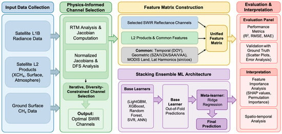
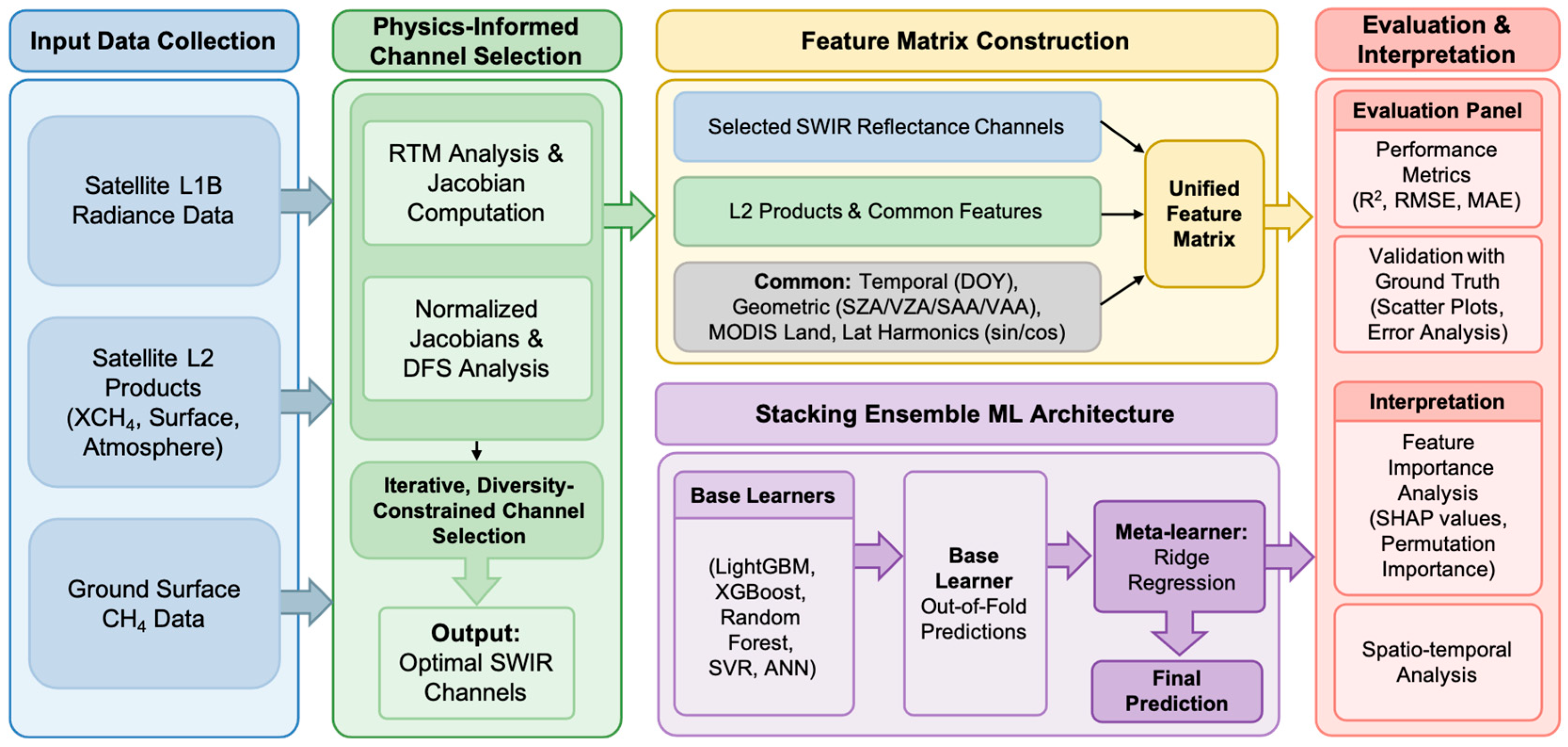
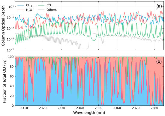
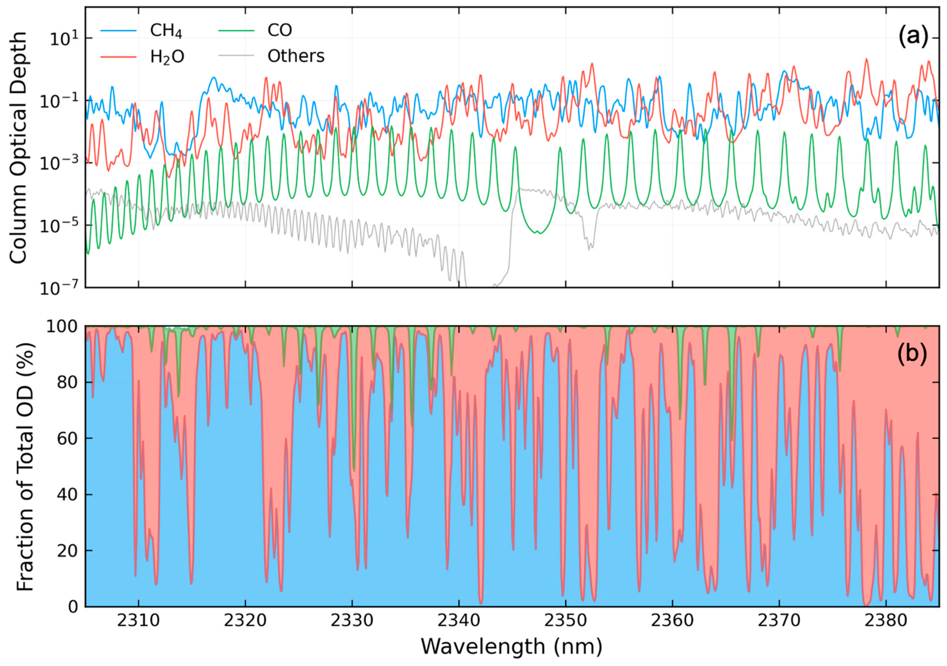
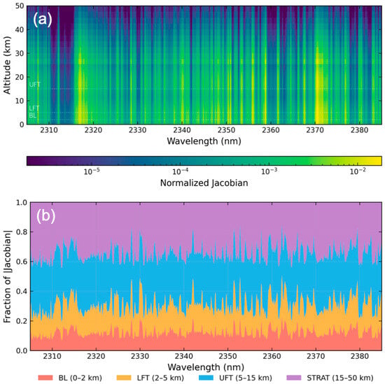
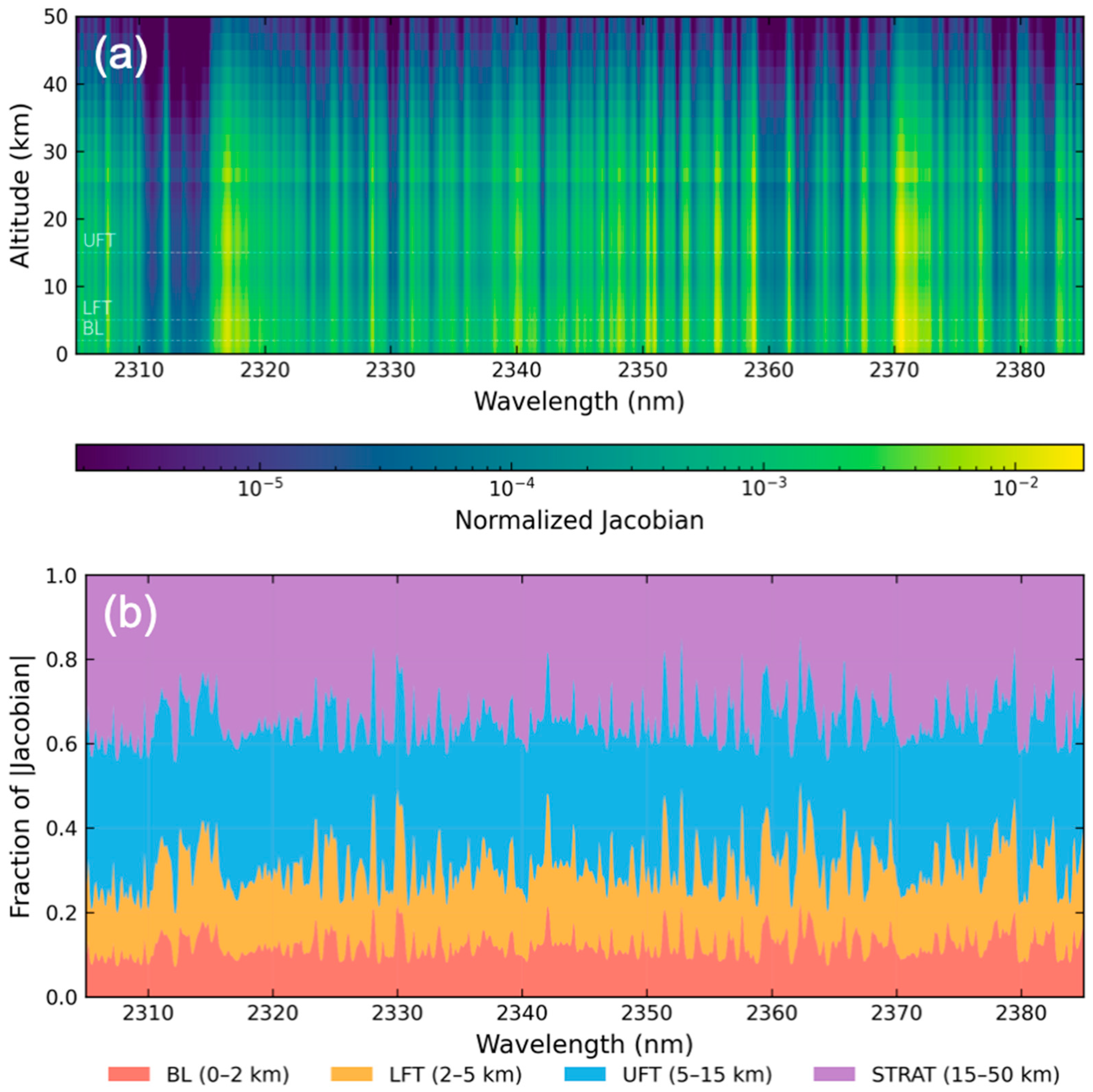
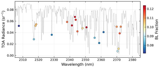
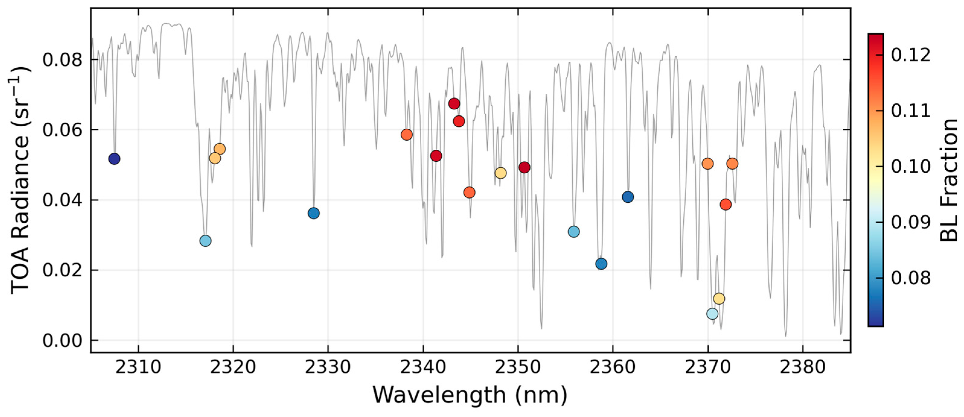
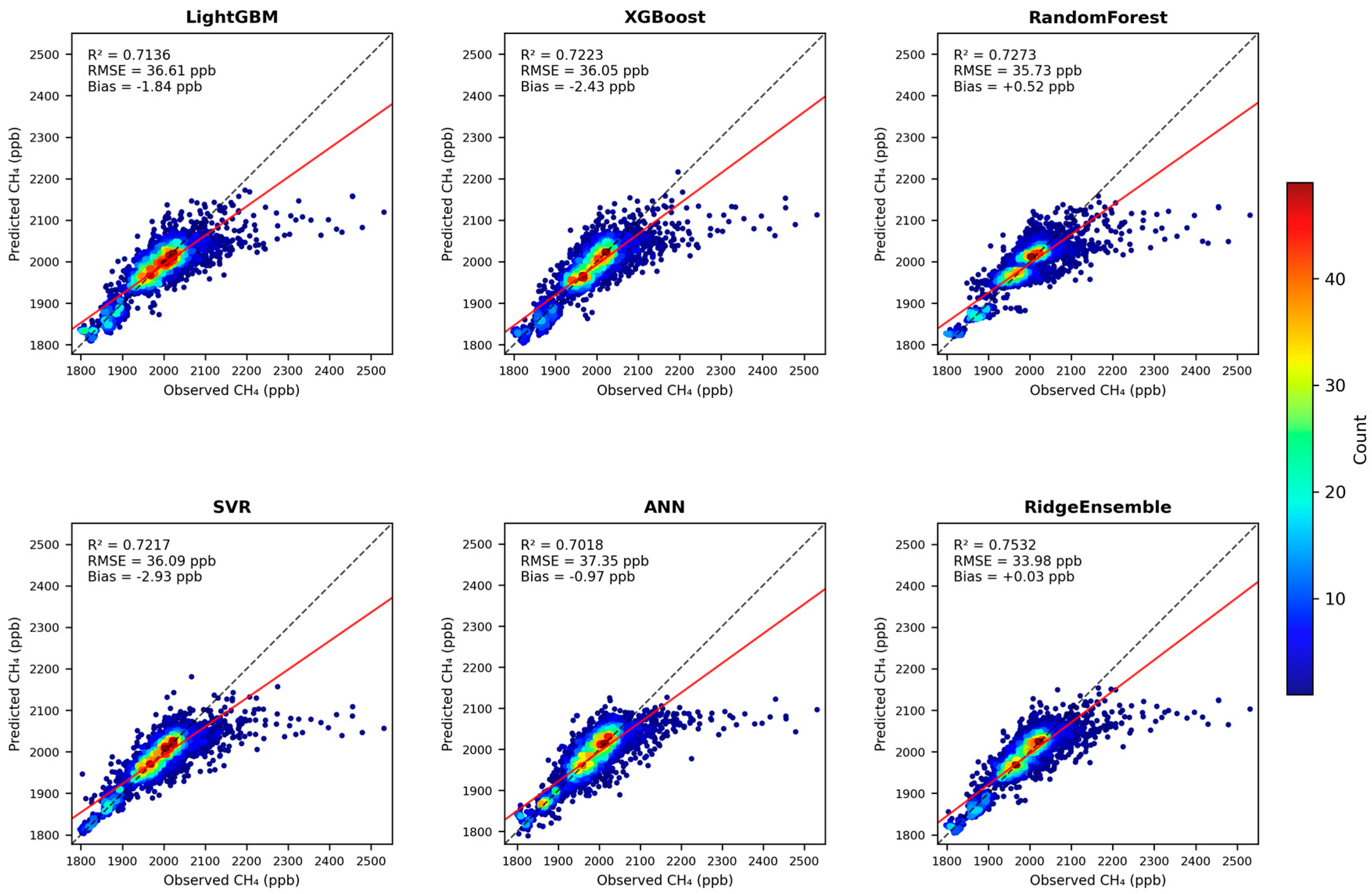
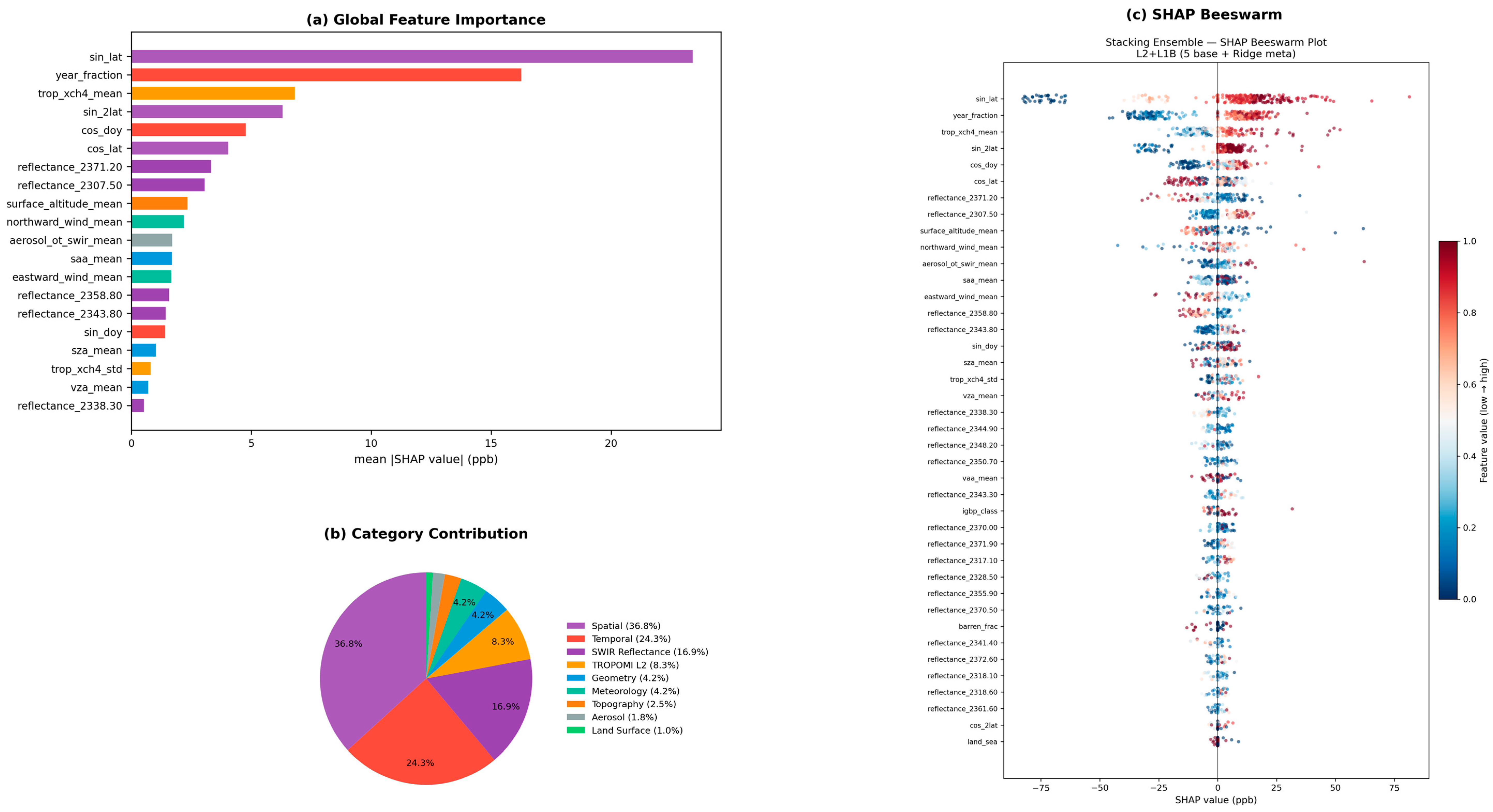
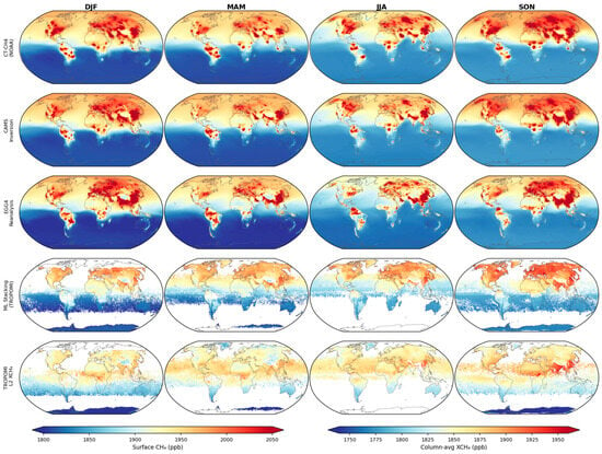
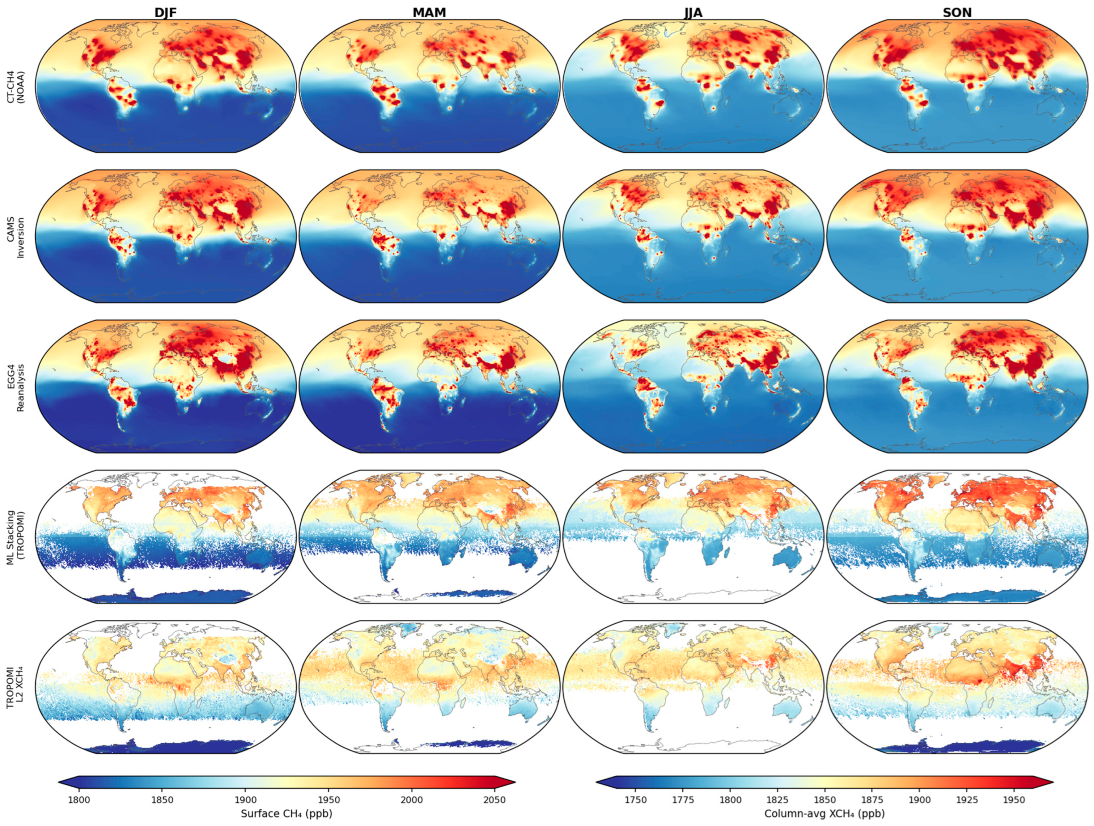

Disclaimer/Publisher’s Note: The statements, opinions and data contained in all publications are solely those of the individual author(s) and contributor(s) and not of MDPI and/or the editor(s). MDPI and/or the editor(s) disclaim responsibility for any injury to people or property resulting from any ideas, methods, instructions or products referred to in the content. |
© 2026 by the authors. Licensee MDPI, Basel, Switzerland. This article is an open access article distributed under the terms and conditions of the Creative Commons Attribution (CC BY) license.