Decomposing Cloud Trends: A Satellite Perspective on Size–Occurrence Compensation and Cloud Overlap Biases in Low-Level Clouds

Highlights

What are the main findings?

• Low-level cloud size changes dominate the spatial pattern of total cloud amount trends but are compensated by corresponding occurrence changes.
• Cloud overlap acts as a confounding factor in passive satellite retrievals, artificially amplifying observed low-level cloud occurrence changes.

What are the implications of the main findings?

• Correcting for cloud overlap bias reveals larger oceanic low-level cloud variations than original records indicate.
• Relying on passive satellite constraints for low-level cloud responses may lead to systematic underestimations of their climate feedbacks.

Abstract

Long-term satellite observations of cloud amount provide critical constraints on climate sensitivity and are essential for reducing uncertainties in climate projections. Different cloud types exert distinct radiative effects and exhibit divergent responses to warming. Yet, their relative contributions to trends in total cloud amount remain inadequately quantified. This study analyzes 17 years (2003–2019) of MODIS observations and reveals that, although global and zonal (60°S–60°N) mean trends in total cloud amount are weak, significant local signals persist. Trend decomposition demonstrates that free-tropospheric cloud occurrence dominates the magnitude of total cloud amount trends, whereas low-level cloud (LowC) size primarily dictates their spatial distribution. Nevertheless, this LowC size signal is substantially suppressed by an opposing LowC occurrence signal, resulting in a significant decoupling between LowC and total cloud amounts. To address the inherent limitations of passive satellite retrievals, we further utilize ERA5 reanalysis data. This data further indicates that approximately half of the trend in LowC occurrence arises from cloud overlap biases unresolved by passive satellite sensors. Correcting for this bias should yield a coherent shift in LowC amount trends over most oceans, suggesting that passive satellite retrievals may have systematically obscured the response of low-level clouds to recent climate change.

1. Introduction

Over recent decades, anthropogenic warming has driven substantial changes in Earth’s climate system [1]. Yet current global climate models continue to yield widely divergent projections, even when driven by identical forcings and despite adequately reproducing historical records [1]. This persistent uncertainty primarily stems from cloud feedbacks, with their complexity and limited representation in models long recognized as a major bottleneck [2,3,4]. At the macrophysical level, the horizontal extent of clouds (i.e., cloud amount) exerts a first-order control on both planetary albedo and outgoing longwave radiation, making it a key determinant of the overall cloud feedback and climate sensitivity [5,6]. Consequently, long-term observational trends in cloud amount are regarded as indispensable constraints for narrowing the range of future climate projections [7,8].

A growing body of literature has documented global and regional changes in total cloud amount over the past decades, often stratified by cloud type to account for their distinct radiative signatures and climate sensitivities [9,10,11,12]. Low-level clouds, for example, are projected to exert a positive feedback through reduced solar reflection as their coverage diminishes [13,14], whereas high clouds tend to yield a near-zero net feedback because their shortwave cooling and longwave warming effects largely cancel out [15]. A common limitation of these assessments, however, lies in their focus on changes in overall cloud amount, without probing the compositional relationships driving such variability. Conceptually, an increase in cloud amount could result from the expansion of existing cloud elements (size variations), from a higher frequency of cloud formation (occurrence variations), or from a combination of both. Distinguishing these two pathways has clear diagnostic value: although dynamics and thermodynamics are intrinsically coupled and jointly influence both components, size variations are more directly exposed to local thermodynamic states such as moisture and stability [16,17], whereas occurrence variations are expected to be more strongly regulated by the persistence of large-scale weather disturbances [18]. However, the relative contributions of size and occurrence changes to observed cloud trends remain poorly quantified.

Implementing this decomposition, however, is hindered by inherent challenges associated with the nature of passive remote sensing records, which present two significant data-quality issues. The first is the well-documented issue of long-term inhomogeneity. Changes in satellite platforms, sensor degradation, and cross-calibration uncertainties can all introduce spurious long-term signals that mask or mimic climatic trends [19,20,21]. The second challenge is that although certain limited algorithms attempt to retrieve multi-layer clouds, standard passive sensors fundamentally struggle to resolve overlapping cloud layers in the vertical column [22,23]. In other words, when a higher cloud layer overlies a lower one, the lower cloud is frequently obscured from detection, leading to a systematic underestimation of low-level cloud occurrence [22]. This limitation extends beyond being a retrieval error of fixed magnitude and fundamentally compromises the ability to physically separate the size and occurrence components of low-level cloud.

To partly address these gaps, in this study, we first apply a decomposition approach to disentangle the size and occurrence components of cloud amount trends using 17 years of observations obtained from MODerate resolution Imaging Spectroradiometer (MODIS). Furthermore, since passive satellite sensors cannot resolve vertical cloud overlap, we employ the fifth generation of the European Centre for Medium-Range Weather Forecasts (ERA5) reanalysis data to assess the impact of cloud overlap on the trends. By leveraging ERA5’s vertically resolved cloud profiles, we aim to distinguish genuinely occurring low-level clouds from those obscured by higher layers, thereby providing a more comprehensive interpretation of satellite-observed cloud trends.

2. Materials and Methods

2.1. Materials

To decompose cloud amount trends and evaluate the vertical overlap bias, two primary datasets spanning January 2003 to December 2019 (17 years) were used in this study. This period was selected to avoid atmospheric anomalies associated with the coronavirus disease pandemic in 2020 and to ensure the orbital stability of the Aqua satellite prior to 2021 [24]. The study domain spans 60°S to 60°N. This latitude band excludes high-latitude areas frequently covered by snow or ice, where high surface albedo compromises cloud retrieval accuracy, while still capturing most global cloud systems. The datasets comprise:

(1)

MODIS observations. We used Collection 6.1 Level-3 daily products from MODIS aboard the Aqua satellite (MYD08-D3, Raytheon/Santa Barbara Remote Sensing (SBRS), Goleta, CA, USA) [25]. This well-calibrated product [26] provides data at a horizontal resolution of 1° × 1°. The uniform Collection 6.1 reprocessing of the entire mission archive, together with the well-documented on-orbit calibration stability of Aqua MODIS [27], supports the homogeneity of the record used here. The use of this single-sensor record also largely avoids artificial discontinuities arising from changes in satellite viewing geometry and instrument characteristics that have been documented in merged multi-satellite cloud records [19]. The variables used include cloud fraction (CF; Cloud_Fraction_Day_Mean) and cloud top pressure (CTP; Cloud_Top_Pressure_Day_Mean). The primary analysis is restricted to daytime measurements; considering nighttime measurements leaves the main conclusions unchanged. The daytime observations therefore correspond to the Aqua overpass, whose local solar time is approximately 13:30 at the equator and shifts progressively earlier northward and later southward, by about 40 min at 60° latitude in either hemisphere, reflecting the satellite’s near-polar, sun-synchronous orbit [28].

(2)

ERA5 reanalysis. To correct for the cloud overlap limitations of passive satellite sensors, we used both hourly [29,30] and monthly [31] averaged reanalysis products from ERA5 [32]. This uniformly gridded product has a native horizontal resolution of 0.25° × 0.25°; it was regridded to 1° × 1° by averaging all 0.25° grid-cell values within each 1° target cell and assigning the mean to the cell center to establish a consistent spatial grid with the MODIS observations. The extracted variables include land–sea mask, monthly averaged vertical velocity and relative humidity at 700 hPa, and hourly cloud cover at 18 pressure levels (1000, 975, 950, 925, 900, 875, 850, 825, 800, 775, 750, 700, 650, 600, 550, 500, 450, and 400 hPa). For ERA5 cloud cover, we used data from the full diurnal cycle (both day and night). This is adopted primarily because our objective is to quantify long-term systematic biases of cloud overlap rather than to quantify instantaneous satellite observational biases. Furthermore, the similarity between MODIS daytime and nighttime trends indicates that diurnal sampling biases in the trend decomposition analyses are secondary. Finally, precisely matching instantaneous fields is also practically infeasible given the fundamental differences between ERA5 and MODIS clouds. Therefore, we used full-diurnal averaging to offer a robust climatological baseline, smoothing transient, high-frequency noise to ensure the quantified cloud overlap bias reflects the fundamental mean atmospheric state. We note that ERA5 does not assimilate any MODIS cloud products used here (i.e., CF and CTP). The only MODIS-derived observations entering ERA5 are polar atmospheric motion vectors, which provide wind information and contain no cloud-property retrievals [32].

2.2. Methods

2.2.1. Data Processing and Statistics

To account for the geometric bias caused by the convergence of meridians toward the poles, all spatial averages presented in this study were computed using area weighting [33]. The area of each grid box was determined by treating the Earth as an oblate spheroid with a radius of 6378.137 km at the equator and 6356.752 km at the poles. Specifically, the area $A_{i,j}$ of a grid cell at longitude index i and latitude index j, centered at longitude ${\lambda }_{i,j}$ and latitude ${\varphi }_{i,j}$, is calculated as:

$$A_{i,j}=M\left({\varphi }_{i,j}\right)N\left({\varphi }_{i,j}\right)\cos {\varphi }_{i,j}∆{\varphi }_{i,j}∆{\lambda }_{i,j}$$

(1)

where $M\left({\varphi }_{i,j}\right)$ and $N\left({\varphi }_{i,j}\right)$ are the meridional and prime vertical radii of curvature of the ellipsoid, respectively, and $∆{\varphi }_{i,j}$ and $∆{\lambda }_{i,j}$ denote the grid spacings in latitude and longitude, respectively (in radians). The area-weighted spatial average $\overline{X}$ of a variable $X$, where $X_{i,j}$ denotes the value of $X$ in the grid cell (i, j), is then computed as:

$$\overline{X}={\displaystyle \frac{{\sum }_i{\sum }_j{X}_{i,j}{A}_{i,j}}{{\sum }_i{\sum }_j{A}_{i,j}}}$$

(2)

Correlations between variables were assessed using the Pearson correlation coefficient (r) [34], which is calculated as the ratio of the covariance between two variables ($x$ and y) to the product of their standard deviations:

$$r_{xy}={\displaystyle \frac{{\sum }_{k=1}^n(x_k-\stackrel{-}{x})(y_k-\stackrel{-}{y})}{\sqrt{{\sum }_{k=1}^n{(x_k-\stackrel{-}{x})}^2}\sqrt{{\sum }_{k=1}^n{(y_k-\stackrel{-}{y})}^2}}}$$

(3)

The coefficient $\mathrm{r}$ provides a dimensionless measure of linear dependency. It assumes a bivariate normal distribution and is sensitive to outliers.

2.2.2. Classification of Cloud Types

Following Zelinka et al. [5], we define three primary cloud type categories based on CF and CTP from MODIS observations: (1) total cloud (TotC), encompassing all samples with CF > 0; (2) low-level cloud (LowC), a subset of TotC with CTP ≥ 700 hPa; and (3) free-tropospheric cloud (FreC), a subset of TotC with CTP < 700 hPa. Note that while Zelinka et al. [5] used a CTP threshold of 680 hPa, we adjust this to 700 hPa to align with the standard pressure levels available in ERA5. Since MODIS is a passive sensor, TotC represents the sum of LowC and FreC visible from the top of the atmosphere.

Analogous cloud types were defined using ERA5 cloud cover to facilitate comparison. Because ERA5 provides three-dimensional (3D) cloud information, classification is based on the corresponding vertical structure. The hourly fields were first averaged to daily means, with all subsequent steps operating on these daily-mean profiles. For each 1° grid cell, the 18-level column was scanned to group consecutive cloudy levels into discrete cloud layers, and the top pressure of each layer was determined. We then define: (1) corrected LowC (corLowC), representing all cloud layers with a top pressure ≥ 700 hPa; (2) mimicked LowC (mimLowC), cloud layers with a top pressure ≥ 700 hPa that have no overlying cloudy layers (i.e., visible to a satellite); and (3) mimicked FreC (mimFreC), cloud layers with a minimum top pressure < 700 hPa. The cloud fraction for these three analogous types is estimated assuming maximum overlap to provide an upper bound on the impact of overlapping layers. Under this assumption, the 2D cloud fraction for a given profile is calculated as the maximum cloud cover value among the corresponding vertical levels, meaning higher-level clouds completely obscure underlying lower-level ones. For example, if a classified profile contains cloudy levels consisting of a higher one of 0.6 and a lower one of 0.3, the estimated 2D cloud fraction is simply max (0.6, 0.3) = 0.6, implying the underlying layer is fully obscured.

2.2.3. Decomposition of Total Cloud Amount Trend

Daily cloud fields for both MODIS and ERA5 were aggregated to annual values, with the annual occurrence frequency defined as the fraction of days in a year on which the cloud type is present. Trends were estimated using ordinary least squares linear regression on these annual mean time (t) series from 2003 to 2019 for each grid cell. To ensure statistical robustness, grid cells were included only if a complete 17-year record was available. Significance tests were performed for all analyses. Given the relatively short time series (17 years), trends are considered statistically significant at the 90% confidence level (α = 0.1) using a two-tailed Student’s t-test. We emphasize that reported p-values measure statistical uncertainty rather than physical importance [35]. Thus, a significant trend does not guarantee a large physical effect, nor does a lack of significance imply the absence of a physical effect [35,36].

For MODIS observations, the TotC amount (Amou) is by definition the sum of contributions from LowC (Amou_LowC) and FreC (Amou_FreC) amounts. Therefore, the trend in the TotC amount (T_Amou−TotC) can be additively decomposed:

$${\mathrm{T}}_{\mathrm{Amou}-\mathrm{TotC}}={\displaystyle \frac{\mathrm{d}({\mathrm{Amou}}_{\mathrm{LowC}}+{\mathrm{Amou}}_{\mathrm{FreC}})}{\mathrm{d}\left(t\right)}}=T_{\mathrm{Amou}-\mathrm{LowC}}+T_{\mathrm{Amou}-\mathrm{FreC}}$$

(4)

where the subscripts denote the cloud type and cloud property. Furthermore, the annual mean cloud amount for each cloud type can be expressed as the product of the corresponding annual mean conditional CF (Size) and occurrence frequency (Occu). Here, Size is defined as the mean CF calculated exclusively for cloudy samples (CF > 0), thereby serving as a proxy for the horizontal extent of the clouds. Applying the product rule of differentiation to this relationship yields the decomposition of the trend for a specific cloud type:

$$T_{\mathrm{Amou}}={\displaystyle \frac{\mathrm{d}\left(\mathrm{Amou}\right)}{\mathrm{d}\left(t\right)}}={\displaystyle \frac{\mathrm{d}(\mathrm{Size}\times \mathrm{Occu})}{\mathrm{d}\left(t\right)}}=\overline{\mathrm{Occu}}\times T_{\mathrm{Size}}+\overline{\mathrm{Size}}\times T_{\mathrm{Occu}}$$

(5)

which demonstrates that the contributions of trends in cloud size and occurrence are weighted by the mean occurrence ($\overline{\mathrm{Occu}}$) and size ($\overline{\mathrm{Size}}$), respectively. In other words, cloud types that are climatologically small or infrequent are less likely to drive substantial trends in cloud amount. By combining the additive and multiplicative relationships, the T_Amou-TotC can be fully partitioned into contributions from size and occurrence trends of both LowC and FreC:

$$T_{\mathrm{Amou}-\mathrm{TotC}}={\overline{{\mathrm{Occu}}_{\mathrm{LowC}}}\times T}_{\mathrm{Size}-\mathrm{LowC}}+{\overline{{\mathrm{Size}}_{\mathrm{LowC}}}\times T}_{\mathrm{Occu}-\mathrm{LowC}}+\overline{{\mathrm{Occu}}_{\mathrm{FreC}}}\times T_{\mathrm{Size}-\mathrm{Fre}}+\overline{{\mathrm{Size}}_{\mathrm{FreC}}}\times T_{\mathrm{Occu}-\mathrm{FreC}}$$

(6)

2.2.4. Regions of Interest

Regional analysis is essential for investigating distinct cloud regimes characterized by different cloud properties and driven by unique mechanisms. Based on surface type, the spatial distribution of TotC amount, and the occurrence of LowC and FreC, we identified five regions of interest (ROIs). To separate land from ocean, we utilized the ERA5 land–sea mask, classifying grid cells with a mask value ≤ 0.2 as ocean and all others as land. We then define: (1) Land, land regions between 60°S and 60°N; (2) Intertropical Convergence Zone (ITCZ), ocean regions between 30°S and 30°N where Occu_FreC > Occu_LowC, indicating a dominance of FreC; (3) StratoCu, ocean regions over 30°S–5°N and 15°N–30°N that satisfy Occu_LowC/Occu_FreC ≥ 3 and Amou_TotC ≥ 65%; (4) Cu, ocean regions between 30°S and 30°N, excluding the ITCZ and StratoCu defined above; and (5) Storm, mid-latitude oceans (60°S–30°S and 30°N–60°N).

The specific latitudinal bands for the StratoCu ROI were selected considering the northward shift in the ITCZ, which is predominantly located north of the equator [37]. The selection criteria for this ROI were designed to isolate persistent stratocumulus decks, with the Occu_LowC/Occu_FreC ratio ensuring the prevalence of LowC, while the TotC amount threshold excludes scattered or broken cloud fields. Sensitivity tests using TotC amount thresholds ranging from 60% to 80% (in 5% increments) yielded consistent results. Collectively, these feature-based ROIs provide a spatial framework to link cloud variations with their underlying regional dynamical mechanisms.

3. Results

3.1. Climatology and Trends of Total Cloud Amount from 17-Year MODIS Observations

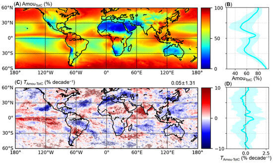
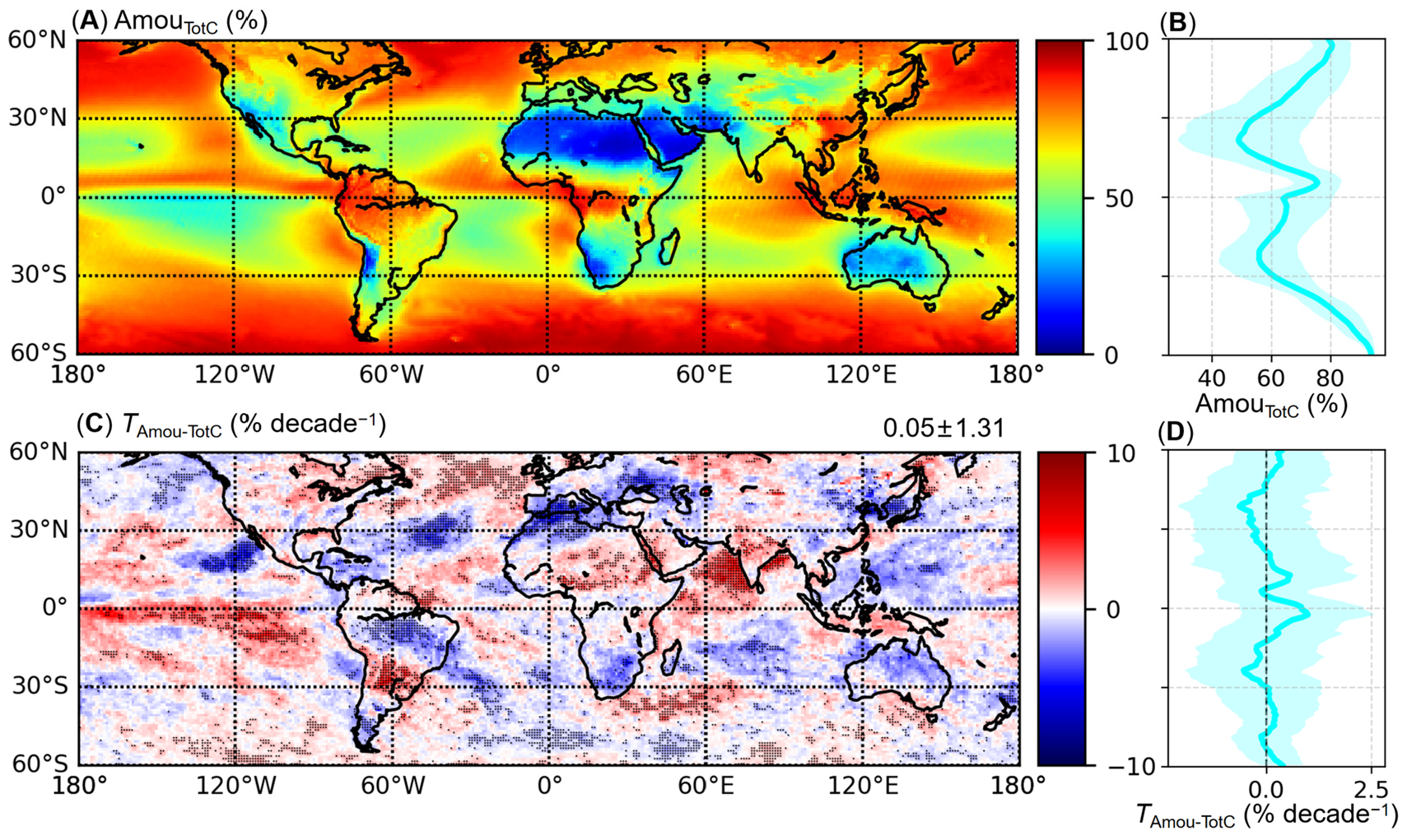
Figure 1 provides a baseline for our analysis, showing the MODIS-observed spatial distributions of the 2003–2019 mean TotC amount and of the corresponding linear trends over the same period.

Figure 1. MODIS observed spatial distributions of the 2003–2019 annual mean TotC amount and the corresponding linear trends. (A) Map of the 17-year climatological mean TotC amount. (B) Zonal-mean profile of the annual mean TotC amount. (C) Map of the TotC amount trend, where black stippling denotes grid cells that are statistically significant at the 90% confidence level (p < 0.1), and the numbers in the top-right corner give the domain-average trend ± 1 s.d.; (D) Zonal-mean profile of the TotC amount trend, where shading in (B,D) denotes ± 1 s.d. of grid-cell values about the zonal mean within each latitude band.

The spatial distribution of the 17-year climatological distribution (Figure 1A) reflects well-established large-scale circulation patterns. In the ITCZ, the ascending branch of the Hadley cell drives deep convective systems, resulting in peak TotC amount zonal means of ~75% (Figure 1B). Conversely, in the subtropics, subsidence by the descending branch of the Hadley circulation suppresses deep cloud formation, yielding relatively lower cloud amounts (zonal means of ~50%). Within the subtropical belt, distinct cloud regimes are evident. Arid continental deserts (e.g., the Sahara and Arabian Deserts) are characterized by minimal cloud cover, while persistent stratocumulus decks dominate the eastern ocean basins, and scattered cumuli characterize the western open oceans [12,38]. At higher latitudes, baroclinic instability drives extratropical cyclone development and storm tracks, generating extensive cloud cover with TotC amount zonal means reaching ~93%.

To assess the temporal evolution of these cloud fields, Figure 1C presents the spatial distribution of TotC amount trends. While the analysis reveals distinct, locally significant trends (black dots in Figure 1C), the zonal mean trends remain relatively small (Figure 1D) due to longitudinal cancelation of opposing signals. Several of these regional patterns align with projected atmospheric circulation changes under global warming. Notably, the negative trends (blue shades in Figure 1C) observed over the Mediterranean and other mid-latitude oceans are consistent with the expansion of the Hadley cell and the poleward displacement of storm tracks [11,38,39,40]. Furthermore, the dipole pattern characterized by decreasing cloud amounts in the western tropical Pacific and increasing cloud amounts in the east suggests a weakening of the Walker circulation [41,42]. Having established the total cloud amount variability from MODIS, we hereafter decompose these trends into contributions from LowC and FreC clouds, and subsequently evaluate the potential overlap bias in satellite observations using ERA5 reanalysis.

3.2. Decomposition of the Total Cloud Amount Trend into LowC and FreC Trends

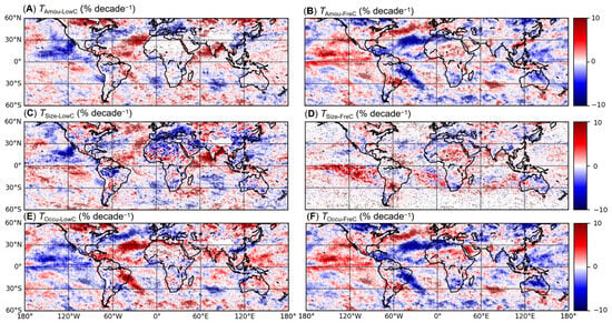
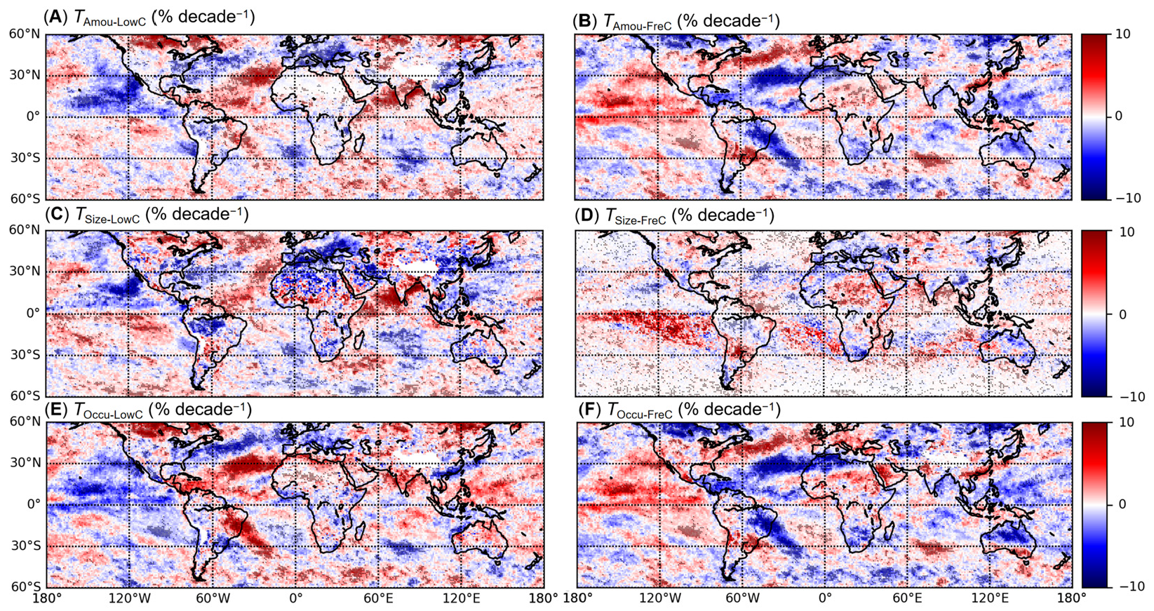
To elucidate the drivers of TotC amount trends, Figure 2 presents the spatial distributions of the trends in cloud amount, size, and occurrence for MODIS LowC (left column) and FreC (right column). While most of these components exhibit significant regional trends, they reveal fundamental differences in their alignment with TotC trends. Notably, the spatial pattern of the LowC size trend closely resembles that of the TotC amount trend (Figure 2C), particularly over the oceans, whereas the FreC size trend remains weak over most areas (Figure 2D). For occurrence, both LowC and FreC exhibit stronger trends than for size and are nearly perfectly anticorrelated (a seesaw relationship, Figure 2E,F). This seesaw is most pronounced in regions of deep organized convection, and its sign is set by the sign of the change in convection depth. In the South Atlantic Convergence Zone, the increase in LowC amount and occurrence (Figure 2A,E) is accompanied by a decrease of comparable magnitude in its FreC counterpart (Figure 2B,F), indicating an exchange across the 700 hPa boundary separating the two categories. In contrast, along the equatorial Pacific ITCZ, a region whose cloudiness is strongly modulated by the El Niño-Southern Oscillation (ENSO), the seesaw reverses sign. There, LowC amount and occurrence decrease (blue in Figure 2A,E) while FreC increases (red in Figure 2B,F), consistent with a deepening of convection that transfers cloudiness to above the 700 hPa level. That the two regions show opposite signs yet a common pivoting level near 700 hPa indicates a vertical redistribution of cloudiness, in which the TotC trends emerge as the residual of opposing LowC and FreC changes. Indeed, over the equatorial Pacific the FreC increase outweighs the LowC decrease, thereby generating the TotC increase over its eastern portion noted in Figure 1C. Collectively, these results suggest a complex physical mechanism wherein FreC and LowC govern different aspects of the overall cloud response to recent climate change through circulation-associated vertical restructuring of the cloud field.

Figure 2. MODIS observed spatial distributions of the 2003–2019 linear trends for LowC and FreC amount, size, and occurrence. (A) LowC amount trend, (B) FreC amount trend, (C) LowC size trend, (D) FreC size trend, (E) LowC occurrence trend, and (F) FreC occurrence trend. Black stippling denotes trends that are statistically significant at the 90% confidence level (p < 0.1).

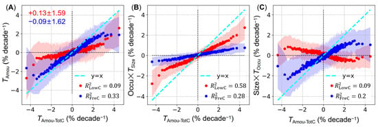
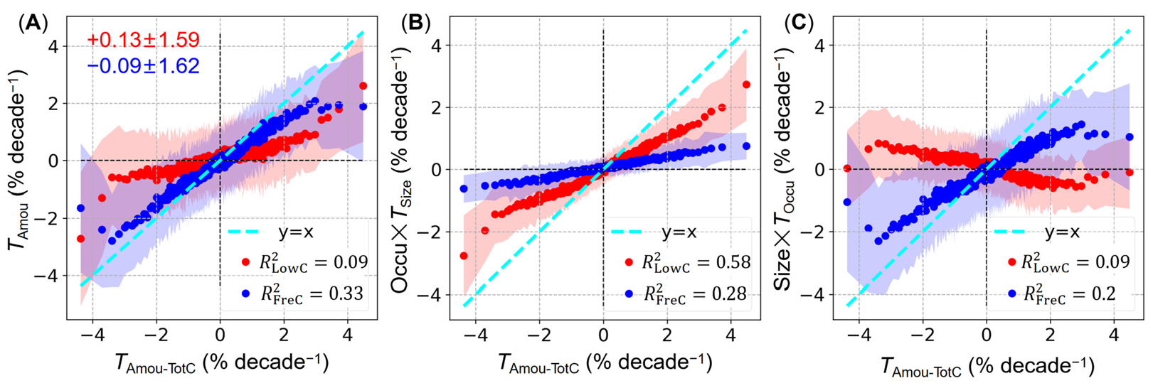
To further quantify the relative contributions of these components, Figure 3 illustrates the weighted terms from the additive (Equation (4)) and multiplicative (Equation (5)) decompositions against TotC amount trends using equal-sample binned scatter plots. For cloud amount trends (Figure 3A), the majority of scatter points for both LowC and FreC are located in the first and third quadrants, indicating that their local trends generally align with the direction of TotC trends. However, in terms of quantitative contribution, FreC trends (blue in Figure 3A) demonstrate a clear dominant role, clustering tightly along the 1:1 reference line (cyan) and explaining ~33% of the TotC trend variance (R² = 0.33, p < 0.01). In contrast, LowC trends exhibit a substantially weaker association with TotC, deviating substantially from the 1:1 line and contributing far less to the explained variance (R² = 0.09, p < 0.01). This contrast highlights that, in terms of cloud amount, FreC is the primary driver of the observed TotC trends, determining both their magnitude and spatial pattern.

Figure 3. MODIS observed dependencies of the 2003–2019 linear trends of LowC (red) and FreC (blue) properties on the TotC amount trends, based on equal-sample binning of TotC trends (each bin contains 150 of the 42,906 valid grid cells, except the final bin). (A) LowC and FreC amount trends versus TotC amount trends; the numbers in the top-left corner give the domain-average trend ± 1 s.d. for LowC and FreC amount. (B) Weighted LowC and FreC size trends versus TotC amount trends. (C) Weighted LowC and FreC occurrence trends versus TotC amount trends. The weighting follows the product-rule decomposition (Equation (6)), such that the terms in (B,C) contribute additively to the amount trend. Cyan lines indicate the one-to-one (x = y) reference. Shading denotes ± 1 s.d. of the trend values about the bin mean within each TotC bin. The coefficient of determination (R²) from the linear regression of LowC and FreC on TotC amount trends is annotated in each panel; all regressions are statistically significant (p < 0.01).

Trends in size (Figure 3B) and occurrence (Figure 3C) further disentangle their compositional relationships with the LowC and FreC amount trends. For FreC, size and occurrence trends vary in tandem. This constructive superposition strengthens the alignment between aggregated FreC amount and TotC trends, but inherently reduces the marginal explanatory power of its individual components, resulting in lower R² values and greater deviations from the 1:1 line than the aggregated trend. Conversely, LowC exhibits a notable compensatory effect, where changes in cloud size are largely offset by opposing changes in occurrence. This size-occurrence compensation weakens the correlation between LowC amount and TotC trends. Despite this, the LowC size trend exhibits the strongest correlation with TotC across all components, explaining ~58% of the variance (R² = 0.58, p < 0.01). However, its regression slope deviates further from the 1:1 line than those of FreC amount and occurrence, indicating a smaller quantitative contribution to the TotC trend magnitude. Thus, distinct physical roles emerge: the LowC size trend dictates the spatial heterogeneity of TotC amount trends (highest R²), whereas the FreC amount trend primarily determines the trend magnitude (best 1:1 fit).

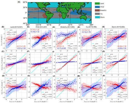
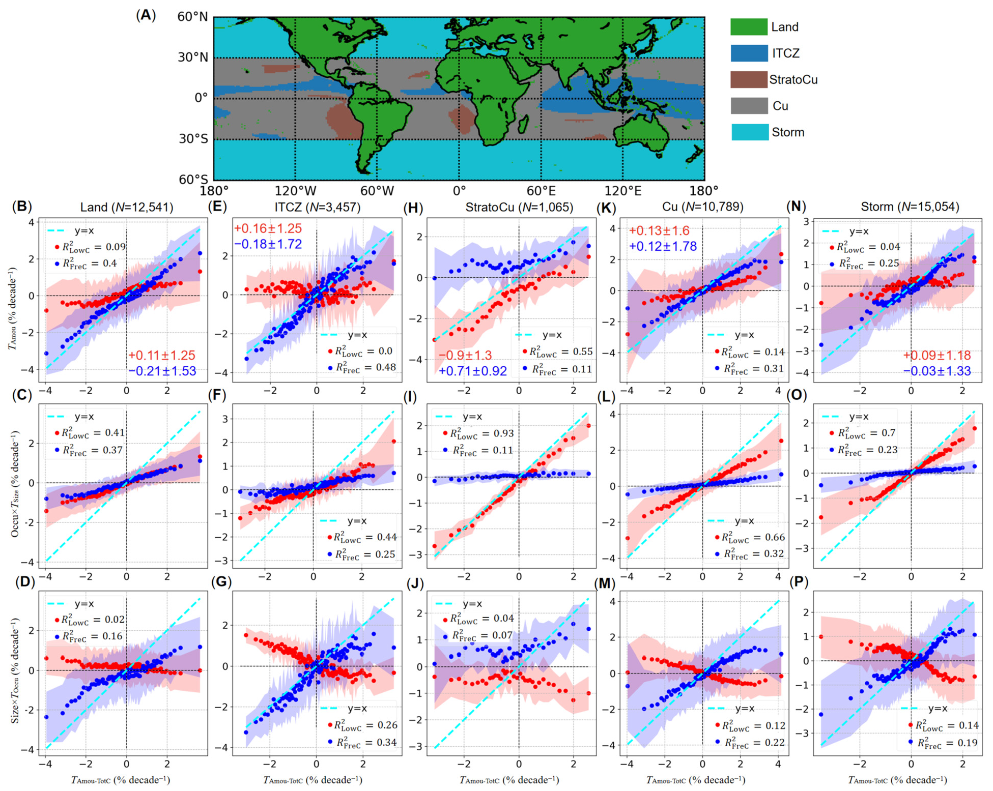
Although the global analysis establishes distinct physical roles of different cloud types and properties, the pronounced spatial heterogeneity in cloud properties and trends (Figure 1) suggests that these mechanisms may operate differently across specific regimes. To evaluate whether our findings hold across regions, we applied the decomposition analysis to each of the five cloud regimes. Figure 4A shows their spatial distribution, and Figure 4B–J present the results for each. Overall, the patterns for the Land, Cu, and Storm ROIs (Figure 4B–D,K–P) are consistent with the global results, whereas those for the ITCZ and StratoCu (Figure 4E–J) deviate markedly.

Figure 4. MODIS observed results for the five ROIs analyzed in this study. (A) Map of the five ROIs. (B–P) Dependence of the 2003–2019 LowC and FreC trends on the TotC amount trends for each ROI (columns: (B–D) for Land; (E–G) for ITCZ; (H–J) for StratoCu; (K–M) for Cu; (N–P) for Storm) and for each property (rows: (B,E,H,K,N), top row, amount trends; (C,F,I,L,O), middle row, weighted size trends; (D,G,J,M,P), bottom row, weighted occurrence trends), plotted as in Figure 3 but with region-specific bin sizes: the count N above each column denotes the number of valid grid cells in each ROI, and each bin contains 150 grid cells for the Land, Cu, and Storm ROIs but 30 for the smaller ITCZ and StratoCu ROIs. All regressions are statistically significant (p < 0.01) except the LowC amount trend for the ITCZ ROI (R² = 0.0017, p = 0.014).

LowC amount trends over the ITCZ ROI show widespread dispersion in the second and fourth quadrants (Figure 4E), and the associated regression is the only one that is not significant at the 1% level (R² = 0.0017, p = 0.014), indicating a decoupling of LowC amount variations from those of TotC. This weakened association is physically consistent with the prevailing deep convective regime of the ITCZ, where TotC variations are largely dictated by deep convective cores and associated anvils, diminishing the relative dominance of boundary-layer low clouds [17,37,43]. Here, the statistical dominance of LowC size also weakens, with FreC amount (Figure 4E, R² = 0.48, p < 0.01) slightly outperforming LowC size (Figure 4F, R² = 0.44, p < 0.01) in explaining TotC variance.

The StratoCu ROI exhibits further distinct deviations (Figure 4H–J). Quantitatively, the domain-mean trends for LowC and FreC amount (Figure 4H, −0.9 ± 1.3 and 0.71 ± 0.92% decade⁻¹) are substantially larger in magnitude than the global means (Figure 3A, 0.13 ± 1.59 and −0.09 ± 1.62% decade⁻¹). Mechanistically, the FreC synergy and LowC compensation effects observed globally are absent. The FreC size trend remains near zero, while the LowC occurrence trend becomes slightly negative, effectively decoupling from trends in their respective amounts. Furthermore, LowC size explains almost all TotC trend variance (Figure 4I, R² = 0.93, p < 0.01) and aligns most closely with the 1:1 line, establishing it as the nearly exclusive determinant of TotC amount trends. These characteristics are again physically consistent with the prevailing cloud regime of the ROI, where stratocumulus decks constitute the primary LowC component [44]. The substantial decrease in LowC, in particular, aligns with an estimated positive feedback associated with stratocumulus clouds [10,45,46,47].

3.3. Assessment of Cloud-Overlap-Induced Biases in LowC Trends and Validation of the Cloud Seesaw Mechanism

Despite the regional heterogeneity highlighted previously, the seesaw relationship between LowC and FreC occurrence trends persists. Because the observed size-occurrence compensation of LowC decouples its amount trend from TotC variations, understanding this seesaw relationship is critical. This first requires addressing a fundamental limitation of MODIS: obscuration by overlapping multi-layer clouds. Due to the top-down viewing geometry of passive sensors, clouds below optically thick upper layers are invisible, hence systematically biasing LowC trend quantifications. For example, patterns in Figure 2 and Figure 3 suggest at least two such effects: (1) the underestimation of occurrence artificially weakens the contribution of the LowC size trend, as the latter is weighted by mean occurrence (Figure 3B); and (2) the detection priority given to upper-layer clouds likely drives the observed seesaw relationship (Figure 2E,F and Figure 3C). Furthermore, because MODIS LowC data are retrieved exclusively when no overlapping clouds are present, this conditional sampling may bias both the estimated mean LowC size and its trend.

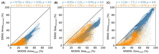
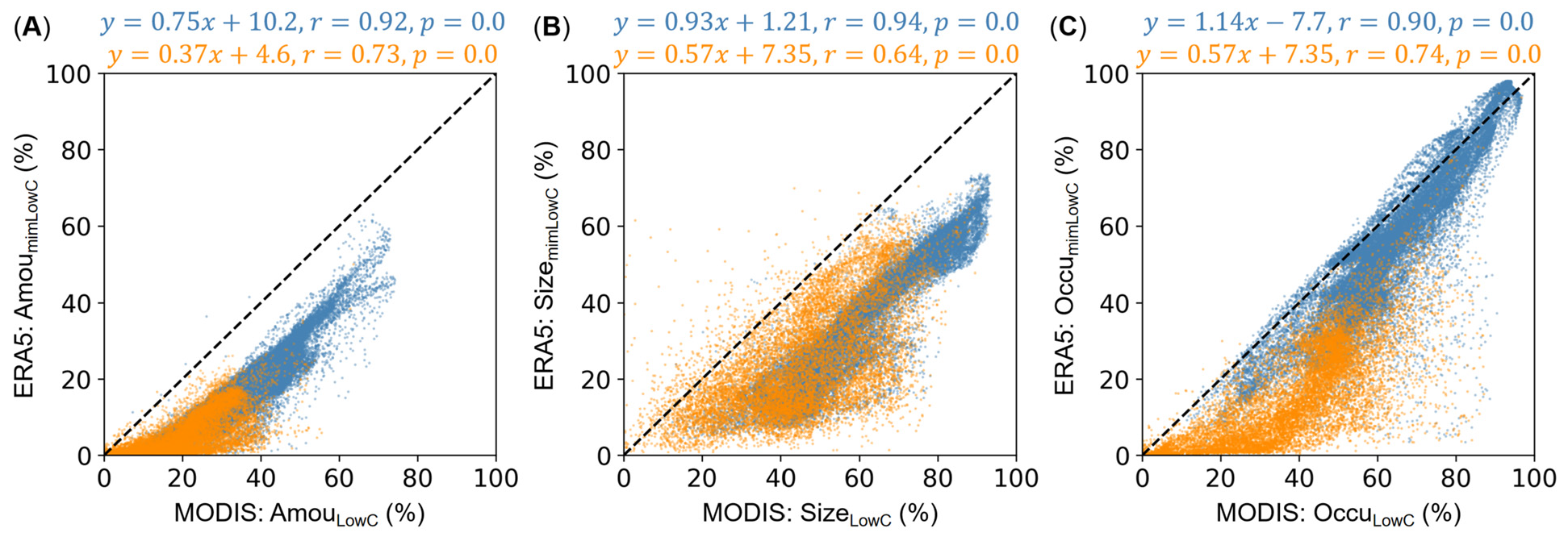
To overcome these overlap limitations, we incorporated ERA5 reanalysis data, which provides 3D cloud fields independent of satellite viewing geometry. We first assessed the suitability of ERA5 by applying the three analogous cloud types defined previously (i.e., mimLowC, mimFreC, and corLowC). Figure 5 compares the annual mean LowC amount, size, and occurrence between MODIS and ERA5, revealing systematic underestimations in the latter. This discrepancy likely stems from methodological differences, particularly ERA5’s application of the maximum-overlap assumption in its 3D cloud fields. By maximizing the vertical obscuration of low-level clouds by upper layers, this assumption inherently depresses the estimated mimLowC values across all three metrics. Despite these underestimations, ERA5 demonstrates strong spatial and temporal agreement with MODIS, particularly over the oceans (r > 0.9), whereas correlations over land are relatively weaker (r < 0.75). Given this discrepancy, we restricted our subsequent overlap analysis to oceanic regions to ensure robustness.

Figure 5. Comparison of the 2003–2019 annual mean LowC properties from MODIS observations against those reconstructed mimLowC properties from ERA5. (A) Cloud amount; (B) cloud size; and (C) cloud occurrence. Yellow and blue dots denote grid cells over land and ocean, respectively. Black dashed lines indicate the one-to-one (x = y) reference. The corresponding ordinary linear regression models are given at the top of each panel.

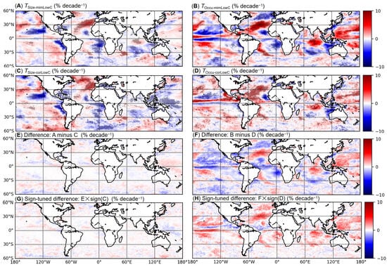
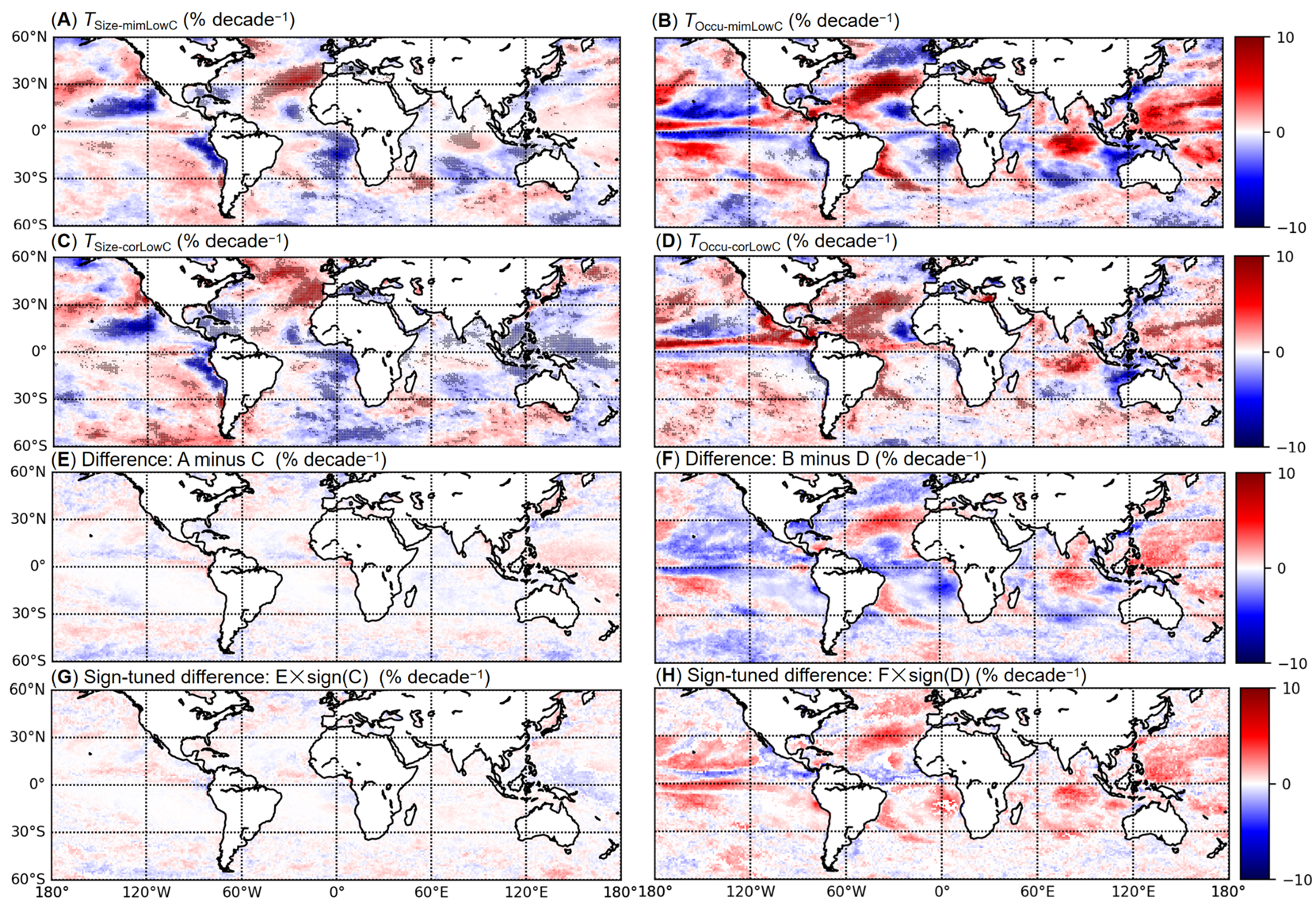
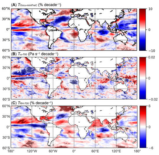
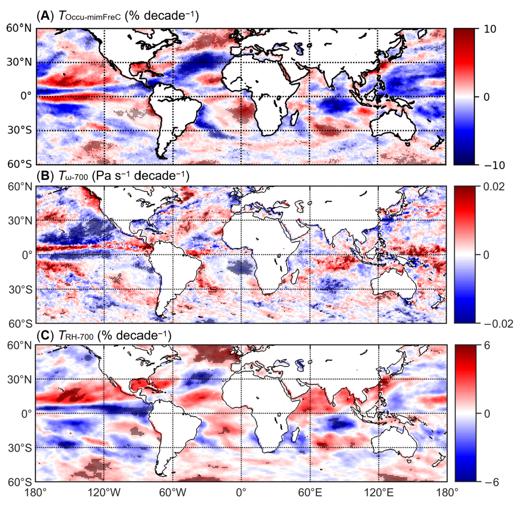
Figure 6 and Figure 7 then present the corresponding ERA5 results, showing the spatial distributions of the mimLowC and corLowC property trends (Figure 6), followed by the FreC occurrence trend and its association with trends in 700 hPa vertical velocity and relative humidity (Figure 7). Over oceans, ERA5 captures the general spatial patterns of MODIS-observed cloud trends despite the systematic underestimation of their magnitudes. This is because the mean-state bias acts largely as a constant offset and does not propagate into the trend estimates and therefore does not invalidate the use of ERA5 for trend analysis. Specifically, the mimLowC size and occurrence trends exhibit patterns highly similar to MODIS retrievals (Figure 6A,B and Figure 2C,E), albeit with a relatively smaller magnitude in the mimLowC size trend. Crucially, this consistency extends beyond individual variables. ERA5 reproduces the mechanistic seesaw relationship between mimLowC and mimFreC occurrence trends (Figure 6A and Figure 7A), mirroring the dynamic observed in MODIS. Collectively, these comparisons substantiate the use of ERA5 data for approximating overlapping cloud biases in MODIS data.

Figure 6. Spatial distributions of the 2003–2019 linear trends from ERA5 for mimLowC and corLowC properties, together with the corresponding differences. (A) mimLowC size trend; (B) mimLowC occurrence trend; (C) corLowC size trend; (D) corLowC occurrence trend; (E) size trend difference ((A) minus (C)); (F) occurrence trend difference ((B) minus (D)); (G) sign-tuned size trend difference ((E) times sign (C)); and (H) sign-tuned occurrence trend difference ((F) times sign (D)). Black stippling in (A–D) denotes trends that are statistically significant at the 90% confidence level (p < 0.1). Grid cells where mimLowC and corLowC trends have opposite signs are masked out in (G,H).

Figure 7. Spatial distributions of the 2003–2019 linear trends from ERA5 for (A) FreC occurrence, (B) vertical velocity at 700 hPa (positive values represent stronger downdrafts or weaker updrafts), and (C) relative humidity at 700 hPa. Black stippling denotes trends that are statistically significant at the 90% confidence level (p < 0.1).

Building upon this validation, we quantified the overlapping bias by calculating the differences in size and occurrence trends between mimLowC and corLowC (Figure 6E,F). The results reveal that the bias associated with the size trend is negligible (Figure 6E), indicating that cloud size dynamics are relatively robust against upper-layer obscuration. In contrast, the bias affecting the occurrence trend is substantial, comparable in magnitude and consistent in spatial distribution with the corLowC signal itself (Figure 6D). This implies that the overlapping effect artificially amplified changes in “real” LowC occurrence across most of the global ocean (red shades in Figure 6H), thereby contributing nearly half of the magnitude of the observed seesaw relationship in MODIS retrievals. Conversely, in the tropical Pacific and Atlantic Oceans, this effect damped the corLowC signal (blue shades in Figure 6H), adding further complexity to the regional manifestation of this dynamic.

Nevertheless, the seesaw relationship between corLowC and mimFreC occurrence trends persists (Figure 6D and Figure 7A), indicating a genuine physical competition between low and non-low cloud regimes rather than a pure artifact of observational obscuration. This relationship is supported dynamically by its spatial consistency with the 700 hPa vertical velocity trends (Figure 7B) and thermodynamically by the accompanying relative humidity trends at the same level (Figure 7C). Specifically, regions of strengthened ascent or weakened descent show increased mimFreC occurrence and decreased corLowC, whereas regions with positive vertical velocity trends show the opposite, with the two sets of regions moistening and drying, respectively. Physically, large-scale ascent promotes deeper convection, increasing both the occurrence and size of FreC, while it also causes low-cloud elements to deepen across the 700 hPa level and convert into FreC, drawing LowC down. These dynamic and thermodynamic conditions thus act in concert: they are consistent with the observed LowC and FreC exchange and jointly determine where it occurs.

4. Discussion

Following the established framework in which cloud amount for each cloud type is expressed as the product of the conditional cloud fraction (i.e., cloud size under cloudy conditions) and the frequency of occurrence (the ratio of cloudy days to all days), our trend decomposition reveals that the magnitude of total cloud amount trends is largely dominated by free-tropospheric cloud amount, particularly by its occurrence, while their spatial distribution is primarily shaped by low-level cloud size. A further, and less intuitive result is that this dominant spatial signal of low-level cloud size is substantially offset by an opposing trend in its occurrence, so that its overall amount trends and total cloud amount trends are effectively decoupled. This decoupling implies that aggregate cloud amount metrics alone cannot reveal the component-level trade-offs that produce them [48]; distinguishing these compositional relationships is therefore necessary for a correct diagnosis of cloud variability. This need is underscored by long-term satellite climate data records, which report statistically significant but strongly region-dependent trends in global cloud amount while remaining silent on the underlying compensation.

However, the inability of passive sensors to resolve overlapping cloud layers fundamentally limits the separation of these compositional relationships, especially the low-level cloud size and occurrence components. Space-based passive radiometers such as MODIS typically provide only a top-of-atmosphere perspective that is heavily weighted toward the uppermost clouds, such that high clouds can partially or totally obscure lower cloud layers. This limitation has been well documented for multi-layer cloud scenes, where the occurrence of overlapping cloud layers ranges from 24% to 40% globally and exceeds 60% in parts of the tropics [49,50]. To overcome this observational limitation inherent in passive satellite retrievals, we leverage ERA5 reanalysis, which provides vertically resolved cloud profiles, as a complementary diagnostic tool to quantify this obscuration bias. Our ERA5-based analysis demonstrates that upper-layer obscuration artificially inflates the perceived low-level cloud occurrence trend by roughly half, whereas the bias associated with the size trend is negligible. This asymmetry is physically consistent with the fact that occurrence is a binary layer-detection problem [51], whereas the size metric is derived from spatially invariant statistics of already-detected low-cloud fields [52].

In the broader context of climate sensitivity, such artificial amplification could lead to a misinterpretation of low-level cloud responses to warming. Given that low-cloud feedback remains the single largest source of inter-model spread in equilibrium climate sensitivity [53], a systematic bias in the observed low-level cloud occurrence trend could systematically skew emergent constraints toward higher (or lower) sensitivity estimates, thereby perpetuating the very uncertainty that observational constraints seek to reduce. Furthermore, while cloud overlap may yield relatively unbiased estimates for top-of-atmosphere radiation, it inevitably introduces significant biases in surface radiation balances [54,55]. This asymmetry arises because shortwave and longwave perturbations induced by upper and lower cloud layers largely cancel when integrated through the atmospheric column but do not cancel at the surface, where each layer’s transmission and emission act on distinct portions of the downwelling flux. Hang et al. [56,57] quantified this effect precisely, showing that the net cloud radiative effect at the surface differs by tens of W m⁻² from passive-only estimates in overlapping-cloud regimes, with the largest biases concentrated in stratocumulus-under-cirrus regions of the eastern subtropical oceans. Given that model evaluation of the surface radiation budget has long relied on both top-of-atmosphere and surface decomposition [58,59], the structure artifact identified here introduces an additional source of uncertainty that should be accounted for alongside existing observational constraints on climate sensitivity.

Despite this overlapping bias, a substantial portion of the observed LowC occurrence trend reflects a genuine, physically coherent signal, as evidenced by its robust alignment with 700 hPa vertical velocity and relative humidity trends. Such a coupling is physically expected, as vertical velocity has long been identified as a primary dynamical control on cloud vertical development and relative humidity as the corresponding thermodynamic control, the two jointly delimiting the environments in which clouds can form and deepen [14,60]. Mechanistically, this is consistent with enhanced ascent and the moistening that accompanies it driving cloud tops above the 700 hPa threshold, reclassifying a fraction of LowC objects as FreC and thereby reducing LowC occurrence. This vertical redistribution of cloud objects is consistent with the observed separation of cloud regimes into shallow and deep convection by free-tropospheric vertical velocity and humidity [61]. Because the total low-level cloud area is not reduced proportionally, the residual LowC population exhibits a larger mean object size. That object-scale and occurrence can respond in opposite directions to a common dynamical forcing is corroborated by cloud-object analyses showing that shallow cumulus and overcast-stratus objects evolve in nearly opposite phases during the Madden-Julian Oscillation [62].

Analogous to how mid-latitude storm dynamics constitute observable signatures of cloud feedback [63], this structurally resolved decomposition offers a potential constraint on future climate projections. However, this transition mechanism is not universally applicable. Stratocumulus clouds are typically capped by strong boundary-layer inversions that physically restrict their vertical development into the free troposphere [44]. Consistent with this constraint, we observed a negligible corLowC occurrence trend over the StratoCu ROI, and the observed cloud changes there are not accompanied by appreciable trends in 700 hPa vertical velocity or relative humidity. Therefore, the apparent seesaw relationship in this region is primarily a retrieval artifact rather than a true dynamical shift.

While our findings advance the understanding of cloud regime transitions, several limitations must be acknowledged and addressed in future research. First, the 17-year MODIS record was selected to provide a robust baseline, but this timescale is insufficient for rigorously constraining decadal-scale climate feedbacks, as cloud trends on sub-30-year timescales can be strongly influenced by internal climate variability, and ENSO in particular has been shown to bias long-term cloud-feedback estimates derived from short satellite records [64,65]. Future studies should integrate long-term coupled model intercomparison projects to better assess these trends within a broader climate context. Second, the MODIS–ERA5 agreement that justifies the use of the latter has been established over the ocean only; the present conclusions should not be extrapolated to land without further evaluation. More generally, while ERA5 serves as a useful proxy for overlapping cloud biases [66,67], it remains a model-based product. To overcome this reliance on reanalysis, future work can incorporate active remote sensing (e.g., spaceborne lidar/radar) to directly resolve vertical cloud profiles and provide independent validation. Third, the transition mechanisms discussed here are unlikely to capture all regional behavior. For instance, processes such as deep convective downdrafts consuming local moisture and suppressing low-level cloud development are not fully resolved by our framework [68,69], and the partitioning itself is contingent on the cloud-object definitions and thresholds adopted, in particular the 700 hPa level used to separate LowC from FreC. In addition, although these relationships are physically coherent, the coincident trends in cloud occurrence, vertical velocity, and relative humidity do not by themselves establish causality. Deepening convection also feeds back on its large-scale environment by transporting moisture and reshaping the divergence field [42]. Disentangling these intertwined processes will require targeted, process-oriented observational and modeling experiments to capture the regional heterogeneity of cloud regime shifts comprehensively.

5. Conclusions

In summary, our analysis of the 17-year MODIS and ERA5 data yields three sets of results. First, total cloud amount trends are locally significant but strongly region-dependent. Opposing regional trends largely cancel in the zonal mean, so global-mean signals remain small, while the surviving regional patterns share spatial signatures with circulation changes projected under global warming, including a poleward shift in the storm tracks and a weakening of the Walker circulation.

Second, decomposing these trends into LowC and FreC components reveals that the two components govern different aspects of the signal. FreC, through its frequency of occurrence in particular, sets the magnitude of the trends, whereas LowC determines their spatial pattern. Within LowC, the decomposition uncovers a genuine compensatory mechanism, in which opposing size and occurrence trends offset each other to obscure the overall amount signal, so that the LowC amount trend is decoupled from the total cloud amount signal. This compensation is robust across the Land, Cu, and Storm regions but breaks down wherever a single process dominates. In the ITCZ, deep convective cores and anvils reduce the leverage of low-level clouds, whereas over the StratoCu region, LowC size alone governs the total cloud amount trend.

Third, a large part of the apparent LowC occurrence trend is observational rather than real. Over the ocean, obscuration by upper-layer clouds artificially introduces a spurious low-level cloud occurrence trend comparable in magnitude to the true dynamical trend, rendering approximately half of the observed MODIS trends artificial, whereas the size trend is essentially unaffected. Despite this substantial bias, the bidirectional dynamical transition of clouds between the lower layer and the free troposphere, associated with large-scale vertical velocity trends and the accompanying moistening, is confirmed as a physical reality. Outside stratocumulus regions, the residual occurrence trend co-varies with 700 hPa vertical velocity and relative humidity and therefore reflects a genuine exchange of cloud objects between the boundary layer and the free troposphere. The critical exception occurs in stratocumulus regions, where the capping effect of strong boundary-layer inversions precludes such vertical exchanges, rendering the apparent LowC–FreC seesaw primarily an artifact of the retrieval.

Together, these results show that total cloud amount trends conceal the compensatory component-level processes that shape them. Ultimately, disentangling these internal dynamics from overlapping observational artifacts is essential for accurately constraining cloud responses and avoiding systematic misinterpretations of cloud feedback in climate projections.

References

- Gulev, S.K.; Thorne, P.W.; Ahn, J.; Dentener, F.J.; Domingues, C.M.; Gerland, S.; Gong, D.; Kaufman, D.S.; Nnamchi, H.C.; Quaas, J.; et al. Changing state of the climate system. In Climate Change 2021: The Physical Science Basis. Contribution of Working Group I to the Sixth Assessment Report of the Intergovernmental Panel on Climate Change; Masson-Delmotte, V., Zhai, P., Pirani, A., Connors, S.L., Péan, C., Berg, S., Caud, N., Chen, Y., Goldfarb, L., Gomis, M.I., et al., Eds.; Cambridge University Press: Cambridge, UK; New York, NY, USA, 2021; pp. 287–422. [Google Scholar] [CrossRef] [Scilit]
- Zelinka, M.D.; Myers, T.A.; McCoy, D.T.; Po-Chedley, S.; Caldwell, P.M.; Ceppi, P.; Klein, S.A.; Taylor, K.E. Causes of Higher Climate Sensitivity in CMIP6 Models. Geophys. Res. Lett. 2020, 47, e2019GL085782. [Google Scholar] [CrossRef] [Scilit]
- Stevens, B.; Sherwood, S.C.; Bony, S.; Webb, M.J. Prospects for narrowing bounds on Earth’s equilibrium climate sensitivity. Earth’s Future 2016, 4, 512–522. [Google Scholar] [CrossRef] [Scilit] [PubMed]
- Sherwood, S.C.; Bony, S.; Dufresne, J.L. Spread in model climate sensitivity traced to atmospheric convective mixing. Nature 2014, 505, 37–42. [Google Scholar] [CrossRef] [Scilit] [PubMed]
- Zelinka, M.D.; Zhou, C.; Klein, S.A. Insights from a refined decomposition of cloud feedbacks. Geophys. Res. Lett. 2016, 43, 9259–9269. [Google Scholar] [CrossRef] [Scilit]
- Ceppi, P.; Brient, F.; Zelinka, M.D.; Hartmann, D.L. Cloud feedback mechanisms and their representation in global climate models. Wiley Interdiscip. Rev. Clim. Change 2017, 8, e465. [Google Scholar] [CrossRef] [Scilit]
- Brient, F.; Schneider, T. Constraints on climate sensitivity from space-based measurements of low-cloud reflection. J. Clim. 2016, 29, 5821–5835. [Google Scholar] [CrossRef] [Scilit]
- Myers, T.A.; Scott, R.C.; Zelinka, M.D.; Klein, S.A.; Norris, J.R.; Caldwell, P.M. Observational constraints on low cloud feedback reduce uncertainty of climate sensitivity. Nat. Clim. Change 2021, 11, 501–507. [Google Scholar] [CrossRef] [Scilit]
- Bony, S.; Dufresne, J.L. Marine boundary layer clouds at the heart of tropical cloud feedback uncertainties in climate models. Geophys. Res. Lett. 2005, 32, 2005GL023851. [Google Scholar] [CrossRef] [Scilit]
- Clement, A.C.; Burgman, R.; Norris, J.R. Observational and model evidence for positive low-level cloud feedback. Science 2009, 325, 460–464. [Google Scholar] [CrossRef] [Scilit] [PubMed]
- Bender, F.A.M.; Ramanathan, V.; Tselioudis, G. Changes in extratropical storm track cloudiness 1983–2008: Observational support for a poleward shift. Clim. Dyn. 2012, 38, 2037–2053. [Google Scholar] [CrossRef] [Scilit]
- Cesana, G.V.; Del Genio, A.D. Observational constraint on cloud feedbacks suggests moderate climate sensitivity. Nat. Clim. Change 2021, 11, 213–218. [Google Scholar] [CrossRef] [Scilit]
- Slingo, A. Sensitivity of the Earth’s radiation budget to changes in low clouds. Nature 1990, 343, 49–51. [Google Scholar] [CrossRef] [Scilit]
- Klein, S.A.; Hall, A.; Norris, J.R.; Pincus, R. Low-cloud feedbacks from cloud-controlling factors: A review. Surv. Geophys. 2017, 38, 1307–1329. [Google Scholar] [CrossRef] [Scilit]
- Kiehl, J.T. On the observed near cancellation between longwave and shortwave cloud forcing in tropical regions. J. Clim. 1994, 7, 559–565. [Google Scholar] [CrossRef] [Scilit]
- Klein, S.A.; Hartmann, D.L. The seasonal cycle of low stratiform clouds. J. Clim. 1993, 6, 1587–1606. [Google Scholar] [CrossRef] [Scilit]
- Garrett, T.J.; Glenn, I.B.; Krueger, S.K. Thermodynamic constraints on the size distributions of tropical clouds. J. Geophys. Res. Atmos. 2018, 123, 8832–8849. [Google Scholar] [CrossRef] [Scilit]
- Mace, G.G.; Benson, S. The vertical structure of cloud occurrence and radiative forcing at the SGP ARM site as revealed by 8 years of continuous data. J. Clim. 2008, 21, 2591–2610. [Google Scholar] [CrossRef] [Scilit]
- Evan, A.T.; Heidinger, A.K.; Vimont, D.J. Arguments against a physical long-term trend in global ISCCP cloud amounts. Geophys. Res. Lett. 2007, 34, L04701. [Google Scholar] [CrossRef] [Scilit]
- Chepfer, H.; Noel, V.; Winker, D.; Chiriaco, M. Where and when will we observe cloud changes due to climate warming? Geophys. Res. Lett. 2014, 41, 8387–8395. [Google Scholar] [CrossRef] [Scilit]
- Norris, J.R.; Evan, A.T. Empirical removal of artifacts from the ISCCP and PATMOS-x satellite cloud records. J. Atmos. Ocean. Technol. 2015, 32, 691–702. [Google Scholar] [CrossRef] [Scilit]
- Li, J.; Huang, J.; Stamnes, K.; Wang, T.; Lv, Q.; Jin, H. A global survey of cloud overlap based on CALIPSO and CloudSat measurements. Atmos. Chem. Phys. 2015, 15, 519–536. [Google Scholar] [CrossRef] [Scilit]
- Marchand, R.; Ackerman, T.; Smyth, M.; Rossow, W.B. A review of cloud top height and optical depth histograms from MISR, ISCCP, and MODIS. J. Geophys. Res. Atmos. 2010, 115, D16206. [Google Scholar] [CrossRef] [Scilit]
- Loeb, N.G.; Johnson, G.C.; Thorsen, T.J.; Lyman, J.M.; Rose, F.G.; Kato, S. Satellite and ocean data reveal marked increase in Earth’s heating rate. Geophys. Res. Lett. 2021, 48, e2021GL093047. [Google Scholar] [CrossRef] [Scilit]
- Platnick, S. MODIS Atmosphere L3 Daily Product. NASA MODIS Adaptive Processing System, Goddard Space Flight Center, USA; NASA Earth Data. 2015. Available online: https://ladsweb.modaps.eosdis.nasa.gov/missions-and-measurements/products/MYD08_D3 (accessed on 18 September 2024).
- Lyapustin, A.; Wang, Y.; Xiong, X.; Meister, G.; Platnick, S.; Levy, R.; Franz, B.; Korkin, S.; Hilker, T.; Tucker, J.; et al. Scientific impact of MODIS C5 calibration degradation and C6+ improvements. Atmos. Meas. Tech. 2014, 7, 4353–4365. [Google Scholar] [CrossRef] [Scilit]
- Xiong, X.; Angal, A.; Chang, T.; Aldoretta, E.; Geng, X.; Link, D.; Sun, J.; Twedt, K.; Wu, A. Aqua MODIS: 20 years of on-orbit calibration and performance. J. Appl. Remote Sens. 2023, 17, 037501. [Google Scholar] [CrossRef] [Scilit]
- Parkinson, C. The Earth-Observing Aqua Satellite Mission: 20 Years and Counting. Earth Space Sci. 2022, 9, e2022EA002481. [Google Scholar] [CrossRef] [Scilit] [PubMed]
- Hersbach, H.; Bell, B.; Berrisford, P.; Biavati, G.; Horányi, A.; Muñoz Sabater, J.; Nicolas, J.; Peubey, C.; Radu, R.; Rozum, I.; et al. ERA5 Hourly Data on Pressure Levels from 1940 to Present. Copernicus Climate Change Service (C3S) Climate Data Store (CDS), 2023. Available online: https://cds.climate.copernicus.eu/datasets/reanalysis-era5-pressure-levels?tab=overview (accessed on 7 January 2025).
- Hersbach, H.; Bell, B.; Berrisford, P.; Biavati, G.; Horányi, A.; Muñoz Sabater, J.; Nicolas, J.; Peubey, C.; Radu, R.; Rozum, I.; et al. ERA5 Hourly Data on Single Levels from 1940 to Present. Copernicus Climate Change Service (C3S) Climate Data Store (CDS), 2023. Available online: https://cds.climate.copernicus.eu/datasets/reanalysis-era5-single-levels?tab=overview (accessed on 7 January 2025).
- Hersbach, H.; Bell, B.; Berrisford, P.; Biavati, G.; Horányi, A.; Muñoz Sabater, J.; Nicolas, J.; Peubey, C.; Radu, R.; Rozum, I.; et al. ERA5 Monthly Averaged Data on Pressure Levels from 1940 to Present. Copernicus Climate Change Service (C3S) Climate Data Store (CDS), 2023. Available online: https://cds.climate.copernicus.eu/datasets/reanalysis-era5-pressure-levels-monthly-means?tab=overview (accessed on 22 October 2026).
- Hersbach, H.; Bell, B.; Berrisford, P.; Hirahara, S.; Horányi, A.; Muñoz-Sabater, J.; Nicolas, J.; Peubey, C.; Radu, R.; Schepers, D.; et al. The ERA5 global reanalysis. Q. J. R. Meteorol. Soc. 2020, 146, 1999–2049. [Google Scholar] [CrossRef] [Scilit]
- Jones, P.D.; Hulme, M. Calculating regional climatic time series for temperature and precipitation: Methods and illustrations. Int. J. Climatol. 1996, 16, 361–377. [Google Scholar] [CrossRef] [Scilit]
- Pearson, K. Note on regression and inheritance in the case of two parents. Proc. R. Soc. Lond. 1895, 58, 240–242. [Google Scholar] [CrossRef] [Scilit]
- Wasserstein, R.L.; Lazar, N.A. The ASA statement on p-values: Context, process, and purpose. Am. Stat. 2016, 70, 129–133. [Google Scholar] [CrossRef] [Scilit]
- Nuzzo, R. Scientific method: Statistical errors. Nature 2014, 506, 150–152. [Google Scholar] [CrossRef] [Scilit] [PubMed]
- Philander, S.G.H.; Gu, D.; Lambert, G.; Li, T.; Halpern, D.; Lau, N.-C.; Pacanowski, R.C. Why the ITCZ is mostly north of the equator. J. Clim. 1996, 9, 2958–2972. [Google Scholar] [CrossRef] [Scilit]
- Norris, J.R.; Allen, R.J.; Evan, A.T.; Zelinka, M.D.; O’Dell, C.W.; Klein, S.A. Evidence for climate change in the satellite cloud record. Nature 2016, 536, 72–75. [Google Scholar] [CrossRef] [Scilit] [PubMed]
- Zelinka, M.D.; Grise, K.M.; Klein, S.A.; Zhou, C.; DeAngelis, A.M.; Christensen, M.W. Drivers of the low-cloud response to poleward jet shifts in the North Pacific in observations and models. J. Clim. 2018, 31, 7925–7947. [Google Scholar] [CrossRef] [Scilit]
- Sanchez-Lorenzo, A.; Enriquez-Alonso, A.; Calbó, J.; González, J.-A.; Wild, M.; Folini, D.; Norris, J.R.; Vicente-Serrano, S.M. Fewer clouds in the Mediterranean: Consistency of observations and climate simulations. Sci. Rep. 2017, 7, 41475. [Google Scholar] [CrossRef] [Scilit] [PubMed]
- Bellomo, K.; Clement, A.C.; Norris, J.R.; Soden, B.J. Observational and model estimates of cloud amount feedback over the Indian and Pacific Oceans. J. Clim. 2014, 27, 925–940. [Google Scholar] [CrossRef] [Scilit]
- Bellomo, K.; Clement, A.C. Evidence for weakening of the Walker circulation from cloud observations. Geophys. Res. Lett. 2015, 42, 7758–7766. [Google Scholar] [CrossRef] [Scilit]
- Houze, R.A., Jr. Mesoscale convective systems. Rev. Geophys. 2004, 42, RG4003. [Google Scholar] [CrossRef] [Scilit]
- Wood, R. Stratocumulus clouds. Mon. Weather Rev. 2012, 140, 2373–2423. [Google Scholar] [CrossRef] [Scilit]
- Brient, F.; Bony, S. Interpretation of the positive low-cloud feedback predicted by a climate model under global warming. Clim. Dyn. 2013, 40, 2415–2431. [Google Scholar] [CrossRef] [Scilit]
- Breul, P.; Ceppi, P.; Nowack, P. The importance of stratocumulus clouds for projected warming patterns and circulation changes. Atmos. Chem. Phys. 2025, 25, 11991–12005. [Google Scholar] [CrossRef] [Scilit]
- Schneider, T.; Kaul, C.M.; Pressel, K.G. Possible climate transitions from breakup of stratocumulus decks under greenhouse warming. Nat. Geosci. 2019, 12, 163–167. [Google Scholar] [CrossRef] [Scilit]
- Stubenrauch, C.J.; Rossow, W.B.; Kinne, S.; Ackerman, S.; Cesana, G.; Chepfer, H.; Di Girolamo, L.; Getzewich, B.; Guignard, A.; Heidinger, A.; et al. Assessment of global cloud datasets from satellites: Project and database initiated by the GEWEX radiation panel. Bull. Am. Meteorol. Soc. 2013, 94, 1031–1049. [Google Scholar] [CrossRef] [Scilit]
- Mace, G.; Zhang, Q.; Vaughan, M.; Marchand, R.; Stephens, G.; Trepte, C.; Winker, D. A description of hydrometeor layer occurrence statistics derived from the first year of merged CloudSat and CALIPSO data. J. Geophys. Res. Atmos. 2009, 114, D00A26. [Google Scholar] [CrossRef] [Scilit]
- Wang, T.; Fetzer, E.J.; Wong, S.; Kahn, B.H.; Yue, Q. Validation of MODIS cloud mask and multilayer flag using CloudSat-CALIPSO cloud profiles and a cross-reference of their cloud classifications. J. Geophys. Res. Atmos. 2016, 121, 11620–11635. [Google Scholar] [CrossRef] [Scilit]
- Haynes, J.M.; Noh, Y.-J.; Miller, S.D.; Haynes, K.D.; Ebert-Uphoff, I.; Heidinger, A. Low cloud detection in multilayer scenes using satellite imagery with machine learning methods. J. Atmos. Ocean. Technol. 2022, 39, 319–334. [Google Scholar] [CrossRef] [Scilit]
- DeWitt, T.D.; Garrett, T.J.; Rees, K.N.; Bois, C.; Krueger, S.K.; Ferlay, N. Climatologically invariant scale invariance seen in distributions of cloud horizontal sizes. Atmos. Chem. Phys. 2024, 24, 109–122. [Google Scholar] [CrossRef] [Scilit]
- Cesana, G.V.; Arouf, A. A reconciled satellite record reveals a negative low cloud feedback over the past 47 years. Geophys. Res. Lett. 2026, 53, e2026GL124158. [Google Scholar] [CrossRef] [Scilit]
- Barker, H.W. Overlap of fractional cloud for radiation calculations in GCMs: A global analysis using CloudSat and CALIPSO data. J. Geophys. Res. Atmos. 2008, 113, D00A01. [Google Scholar] [CrossRef] [Scilit]
- Ahlgrimm, M.; Forbes, R. The impact of low clouds on surface shortwave radiation in the ECMWF model. Mon. Weather Rev. 2012, 140, 3783–3794. [Google Scholar] [CrossRef] [Scilit]
- L’Ecuyer, T.S.; Hang, Y.; Matus, A.V.; Wang, Z. Reassessing the effect of cloud type on Earth’s energy balance in the age of active spaceborne observations. Part I: Top of atmosphere and surface. J. Clim. 2019, 32, 6197–6217. [Google Scholar] [CrossRef] [Scilit]
- Hang, Y.; L’Ecuyer, T.S.; Henderson, D.S.; Matus, A.V.; Wang, Z. Reassessing the effect of cloud type on Earth’s energy balance in the age of active spaceborne observations. Part II: Atmospheric heating. J. Clim. 2019, 32, 6219–6236. [Google Scholar] [CrossRef] [Scilit]
- Cole, J.; Barker, H.W.; Loeb, N.G.; Von Salzen, K. Assessing simulated clouds and radiative fluxes using properties of clouds whose tops are exposed to space. J. Clim. 2011, 24, 2715–2727. [Google Scholar] [CrossRef] [Scilit]
- Wild, M. Short-wave and long-wave surface radiation budgets in GCMs: A review based on the IPCC-AR4/CMIP3 models. Tellus A 2008, 60, 932–945. [Google Scholar] [CrossRef] [Scilit]
- Norris, J.R.; Iacobellis, S.F. North Pacific cloud feedbacks inferred from synoptic-scale dynamic and thermodynamic relationships. J. Clim. 2005, 18, 4862–4878. [Google Scholar] [CrossRef] [Scilit]
- George, G.; Stevens, B.; Bony, S.; Klingebiel, M.; Vogel, R. Observed impact of mesoscale vertical motion on cloudiness. J. Atmos. Sci. 2021, 78, 2413–2427. [Google Scholar] [CrossRef] [Scilit]
- Xu, K.M.; Wong, T.; Dong, S.; Chen, F.; Kato, S.; Taylor, P.C. Cloud object analysis of CERES Aqua observations of tropical and subtropical cloud regimes: Evolution of cloud object size distributions during the Madden-Julian Oscillation. J. Quant. Spectrosc. Radiat. Transf. 2017, 188, 148–158. [Google Scholar] [CrossRef] [Scilit]
- Tselioudis, G.; Rossow, W.B. Climate feedback implied by observed radiation and precipitation changes with midlatitude storm strength and frequency. Geophys. Res. Lett. 2006, 33, 2005GL024513. [Google Scholar] [CrossRef] [Scilit]
- Marotzke, J.; Forster, P. Forcing, feedback and internal variability in global temperature trends. Nature 2015, 517, 565–570. [Google Scholar] [CrossRef] [Scilit] [PubMed]
- Liu, H.; Koren, I.; Altaratz, O.; Mu, S. ENSO contribution to the assessment of long-term cloud feedback on global warming. Atmos. Chem. Phys. 2026, 26, 5589–5602. [Google Scholar] [CrossRef] [Scilit]
- Yao, B.; Teng, S.; Lai, R.; Xu, X.; Yin, Y.; Shi, C.; Liu, C. Can atmospheric reanalyses (CRA and ERA5) represent cloud spatiotemporal characteristics? Atmos. Res. 2020, 244, 105091. [Google Scholar] [CrossRef] [Scilit]
- Liu, H.; Koren, I.; Altaratz, O.; Chekroun, M.D. Opposing trends of cloud coverage over land and ocean under global warming. Atmos. Chem. Phys. 2023, 23, 6559–6569. [Google Scholar] [CrossRef] [Scilit]
- Johnson, R.H.; Nicholls, M.E. A composite analysis of the boundary layer accompanying a tropical squall line. Mon. Weather Rev. 1983, 111, 308–319. [Google Scholar] [CrossRef] [Scilit]
- Schiro, K.A.; Neelin, J.D. Tropical continental downdraft characteristics: Mesoscale systems versus unorganized convection. Atmos. Chem. Phys. 2018, 18, 1997–2010. [Google Scholar] [CrossRef] [Scilit]
Disclaimer/Publisher’s Note: The statements, opinions and data contained in all publications are solely those of the individual author(s) and contributor(s) and not of MDPI and/or the editor(s). MDPI and/or the editor(s) disclaim responsibility for any injury to people or property resulting from any ideas, methods, instructions or products referred to in the content. |
© 2026 by the authors. Licensee MDPI, Basel, Switzerland. This article is an open access article distributed under the terms and conditions of the Creative Commons Attribution (CC BY) license.