


Highlights
What are the main findings?
- The proposed STGAF-Net effectively integrates radar and surface wind speed data through two-stage gated fusion, local–global encoding, and lightweight non-recurrent temporal modeling.
- An adaptive wind-speed-weighted Huber loss is designed to dynamically adjust the Huber threshold based on the batch-wise error distribution, thereby mitigating performance degradation for samples exceeding high-wind-speed thresholds.
What are the implications of the main findings?
- This model framework helps to address these limitations of existing deep learning models, mitigating performance degradation at high-wind-speed thresholds.
- Accurate and efficient wind speed nowcasting can support traffic management, emergency response, and wind-risk assessment.
Abstract
Accurate wind speed nowcasting is critical for wind-risk assessment, traffic management, and emergency response. However, existing deep learning methods still suffer from inadequate multi-source meteorological data fusion, multi-step error accumulation, and performance decay at high-wind-speed thresholds. To address these issues, this paper proposes STGAF-Net, a multi-source spatiotemporal gated adaptive fusion network. It uses radar reflectivity and surface wind speed as complementary inputs, employs collaborative local–global encoding to capture local details and long-range spatial dependencies, and adaptively integrates multi-source features through stage-wise gating. Temporally, non-recurrent spatiotemporal modeling dynamically adjusts the contribution of each historical time step based on sequence evolution and time intervals, enabling parallel prediction of future wind fields. This end-to-end framework effectively bolsters spatial structure preservation and long-range dependency modeling for severe winds. The experimental results demonstrate that STGAF-Net achieves the strongest overall performance among seven learning-based baselines and a non-learning persistence forecast on two datasets, particularly at high-wind-speed thresholds and at later lead times within the 2-h nowcasting horizon.
1. Introduction
Severe convective winds are generally triggered by meso- and small-scale convective systems and are characterized by strong localization, rapid development, a short duration, and high disaster risk [1,2,3]. Surface wind speeds can change markedly within a short period and exhibit complex spatial propagation and local intensification [2]. Fine-grid, short-lead forecasts of future wind speed distributions can extend warning lead times and provide spatially targeted guidance for transportation, outdoor facility protection, and emergency response [4]. However, wind-field evolution is jointly affected by convective structure, environmental flow, and surface conditions. A single station or meteorological variable therefore cannot fully describe the initiation, movement, and decay of strong-wind areas [5].
Traditional wind speed nowcasting methods mainly include numerical weather prediction, statistical models, and shallow machine learning approaches [6,7]. In operational nowcasting verification, Eulerian persistence is commonly used as a simple non-learning reference forecast. It assumes that the latest observed field remains unchanged at all subsequent lead times and can remain competitive over very short forecast horizons because of the temporal continuity of meteorological fields [8]. Numerical weather prediction describes wind-field evolution by solving atmospheric dynamical and thermodynamic equations and therefore has a clear physical basis. However, high-resolution simulations place substantial demands on initial-condition quality and computing resources [9]. ARIMA, support vector regression, and related hybrid models can extract patterns from historical sequences and have been widely applied to single-site and short-term prediction [10,11,12]. Nevertheless, these methods generally depend on linear assumptions, handcrafted features, or limited representations of spatial relationships, making them poorly suited to the strong nonlinearity and complex spatiotemporal coupling of regional wind fields [13,14].
In recent years, deep learning has attracted extensive attention in wind speed nowcasting because of its ability to learn representations directly from meteorological data [15]. LSTM [16], GRU, and their convolutional variants model temporal dependencies through gating mechanisms [17]. ConvLSTM [18], PredRNN++ [19], and MIM [20] further combine spatial feature extraction with sequence evolution to learn spatiotemporal variations in meteorological fields. Fully convolutional networks and attention-based models have also been introduced for spatiotemporal prediction, using parallel computation to enlarge the effective receptive field and reduce reliance on stepwise recurrence. SimVP [21] is a purely CNN-based spatiotemporal prediction model with an encoder–translator–decoder architecture. EarthFarseer [22], a representative Transformer model, combines local convolution with a global Fourier Transformer to capture both global and local interactions in spatiotemporal dynamical systems and has shown substantial potential in meteorological nowcasting. Although these studies improve the representation of nonlinear evolution, recurrent structures may still accumulate errors over longer forecast horizons. Local convolution alone cannot adequately establish relationships between distant regions, whereas direct global self-attention incurs high computational and memory costs.
Multi-source meteorological observations provide richer information for addressing these limitations. Zhang et al. [23] proposed a deep learning model based on a convolution-self-attention architecture and integrated meteorological variables from different modalities through a spatiotemporal fusion module, achieving high-accuracy intelligent forecasts of short-term low-altitude wind fields. More recently, Geng et al. [24] proposed MSF-PhyDRNN, a physics-driven recurrent network that integrates radar reflectivity and surface wind fields through multi-source feature fusion for short-term thunderstorm-gale nowcasting. Because it addresses the same target variable using comparable multi-source observations, MSF-PhyDRNN constitutes the most closely related learning-based reference for the present study. For wind speed nowcasting, surface wind speed directly describes the state of the near-surface wind field, while weather radar reflectivity characterizes the location, morphology, intensity, and evolution of convective systems and is valuable for identifying convectively induced gusts [25]. The two data sources are therefore strongly complementary in physical meaning and spatiotemporal behavior. However, their statistical distributions and informative content differ. Simple concatenation or uniform weighting can propagate irrelevant echoes, background noise, and redundant wind responses into the prediction network [24,26]. The contribution of radar information also varies by processing stage. During spatial encoding, radar data are well suited to locating and correcting wind structures associated with convection; during temporal evolution, they can provide dynamic precursors of future wind speed changes. Multi-source fusion should therefore perform content-dependent spatial selection and temporal correction rather than a single fusion operation at one location [27].
Existing approaches also face two related spatiotemporal modeling challenges. First, strong-wind cores, local gradients, and echo boundaries require fine neighborhood features, whereas the organization and propagation of convective systems and their influence across regions require long-range spatial relationships. Frequent downsampling reduces computation but may blur strong-wind boundaries and isolated high-value regions. Conversely, global modeling at the original resolution can be prohibitively expensive. Second, historical observations contribute unequally to future wind speeds. Fixed temporal weights cannot distinguish rapidly developing periods from stable periods, while stepwise recurrence propagates errors from one prediction to subsequent steps. Wind speed nowcasting therefore requires a model that preserves local details, captures global context at moderate computational cost, and dynamically selects important historical information according to inter-frame changes.
To address these challenges, we propose the multi-source spatiotemporal gated adaptive fusion network, STGAF-Net. The network separately encodes radar reflectivity and surface wind speed and applies gated fusion after spatial encoding and temporal evolution to exploit radar information at both stages. A local convolution branch preserves strong-wind cores, local gradients, and echo boundaries. A compressed global attention branch retains full-resolution queries while compressing keys and values, thereby establishing long-range spatial relationships at lower computational cost. Learnable weights adaptively combine the two branches. To avoid fixed temporal weighting and recurrent error accumulation, the non-recurrent Difference-Aware Peripheral Time Units (DAP-TUs) process historical sequences in a unified time–channel space, using decomposed large-kernel convolutions to capture propagation patterns from local cores to surrounding regions and temporal difference gating to adaptively weight historical time steps according to feature changes and time intervals. We further design an Adaptive Wind-speed-weighted Huber (AWH) loss, which uses a dynamic threshold and wind-speed-dependent weights to emphasize high-wind-speed regions. The resulting end-to-end framework improves the preservation of strong-wind spatial structures and the modeling of long-term dependencies.
The main contributions of this work are summarized as follows:
- We propose a dual-branch local–global encoder with a two-stage gated adaptive fusion mechanism. It preserves fine-scale strong-wind structures through local convolutions and captures long-range spatial dependencies through compressed global attention. Two gated fusion stages then adaptively integrate radar reflectivity and surface wind speed features after spatial encoding and temporal evolution, respectively.
- We design the non-recurrent Difference-Aware Peripheral Time Units (DAP-TUs). Decomposed large-kernel convolutions enlarge the effective receptive field, and dynamic weights derived from inter-frame content differences and time intervals emphasize important historical time steps. The unit processes the complete historical sequence in parallel and reduces error accumulation caused by stepwise recurrence.
- We introduce an Adaptive Wind-speed-weighted Huber (AWH) loss. By dynamically adjusting the Huber threshold and assigning greater loss weights to samples exceeding high-wind-speed thresholds, AWH accurately fits small errors, robustly suppresses large errors, and mitigates performance degradation under high-wind-speed conditions.
- Comprehensive experiments against seven representative learning-based baselines and a non-learning persistence forecast on the Jiangsu and Convective Gusts datasets demonstrate the effectiveness of STGAF-Net, particularly at high wind-speed thresholds and longer forecast lead times.
2. Methodology
2.1. Problem Definition
The evolution of wind fields is driven by complex interactions among multiple atmospheric factors. This study focuses on nowcasting across continuous grid-based wind fields, a task inherently formulated as a high-dimensional spatiotemporal modeling problem spanning spatial (longitude, latitude), temporal, and meteorological variable dimensions. Specifically, the target geographic domain is discretized into regular grid cells, with each cell functioning as a spatial observation node that tracks dynamic meteorological variations over time. To capture these underlying dynamics accurately, we integrate weather radar reflectivity and surface wind speed as complementary multi-source inputs. At any given time step , the observation field is represented by a tensor , where B is the batch size, C denotes the channel dimension of meteorological variables (, corresponding to radar reflectivity and wind speed), and denotes the spatial grid dimensions. The objective of wind speed nowcasting is to predict the most probable future wind speed sequence of length q, denoted as , conditioned on the historical sequence of the preceding s observations .
2.2. STGAF-Net Overall Architecture
The overall architecture of STGAF-Net is shown in Figure 1. The network consists of five main components: a dual-branch encoder, a spatial fusion module, Difference-Aware Peripheral Time Units (DAP-TUs), a temporal fusion module, and a decoder. To accurately predict wind speeds over the 0–2 h nowcasting horizon, the model integrates surface wind fields and radar reflectivity. As defined above, the historical meteorological tensor containing two variables (), , is used directly as the initial input, where B denotes the batch size, T denotes the number of time steps, and H and W denote the numbers of grid points in the study domain. The wind and radar sequences are first processed by two parallel encoders to obtain source-specific spatial representations. The Spatial Fusion Module then uses the radar representation to selectively enhance the wind features through spatial gating. Subsequently, the two feature sequences are independently processed by the DAP-TUs to capture their temporal evolution. The Temporal Fusion Module further incorporates temporal precursor information from the evolving radar features into the wind representation through channel gating. Finally, the decoder transforms the fused spatiotemporal representation into wind speed fields for multiple future time steps.
Figure 1.
The overall architecture of STGAF-Net.
2.3. Encoder–Decoder
To extract spatial information at different scales from wind fields and radar reflectivity, we design the local–global dual-branch encoder shown in Figure 2. The local convolution and compressed global attention branches operate in parallel to capture multiscale spatial features.
Figure 2.
The structure of the encoder–decoder.
For the input field at any given time step, , a shallow mapping unit consisting of a convolution, batch normalization, and a ReLU activation function is first employed for initial encoding. This unit maps the raw meteorological variable into a unified feature space:
The embedding layer increases the channel dimension to provide sufficient representational capacity for subsequent attention and channel mixing. Meanwhile, the local convolution performs preliminary denoising and neighborhood feature extraction before the features enter the two branches. Subsequently, is fed simultaneously into the local convolution branch and the compressed global attention branch.
2.3.1. Local Convolution Branch
The local convolution branch uses depthwise separable convolution to extract neighborhood information. A depthwise convolution first processes each feature channel independently, capturing local textures, gradient changes, and spatial boundaries at low computational cost. A pointwise convolution then enables information exchange across channels. The local feature extraction process is expressed as follows:
where denotes a depthwise convolution and denotes a pointwise convolution. Compared with standard convolution, this structure substantially reduces the parameter count and computational cost while preserving local representation capacity. The residual connection passes the original embedded features directly to the branch output, helping preserve wind-field boundaries, isolated high-value points, and fine radar-echo textures while improving gradient propagation through the deep network.
2.3.2. Global Attention Branch
Inspired by the Compressed Vision Transformer (CViT) proposed by Yuan et al. [28], we introduce a compressed global attention branch into the encoder. This branch retains the full spatial resolution of query () while compressing only key () and value (). It therefore reduces spatial redundancy in wind and radar features while maintaining sensitivity to important locations and long-range context. The input features are first layer-normalized, after which depthwise and pointwise convolutions generate the query, key, and value features:
where denotes a depthwise convolution that extracts local spatial structures, and denotes a pointwise convolution that mixes channel information. Wind fields and radar reflectivity generally exhibit strong spatial continuity, and adjacent grid cells contain redundant information. retains the response at every original location and therefore preserves the full spatial resolution. and are spatially compressed to obtain compact global context:
where denotes bilinear interpolation. The compressed and have smaller spatial dimensions, whereas retains the same resolution as the original features. Global attention is then computed from the compressed keys and values, and the aggregated result is projected through depthwise and pointwise convolutions:
where d is the feature dimension of each attention head and is a learnable relative positional bias that represents the direction and distance between spatial locations. Finally, the attention features are combined with the input through a residual connection, and a feed-forward network further extracts nonlinear inter-channel relationships:
By retaining full-resolution queries and compressing keys and values, this branch models long-range spatial relationships in wind and radar features with lower computational and memory costs. It provides a representation with complete positional responses and global context for subsequent local–global feature fusion.
2.3.3. Adaptive Local–Global Fusion
After extracting local and global features, we introduce the learnable coefficients and to fuse the two branches:
where and control the contributions of local and global information to the encoded representation, respectively. The fused features are then passed through a convolution, batch normalization, a ReLU activation, and a convolution to obtain the encoder output:
This design adaptively balances local details and long-range dependencies. The decoder uses the same local–global dual-branch unit but processes only the fused target wind-field features. A final convolution projects the hidden representation onto a single-channel wind speed field. The encoder maintains the original spatial resolution throughout, reducing the blurring of strong-wind boundaries caused by downsampling.
The decoder mirrors the encoder and performs spatiotemporal reconstruction only on the target wind-field features after multi-source fusion. Subsequently, a final convolution performs linear projection, and the resulting features are rearranged as to produce single-channel wind speed fields at multiple future time steps.
2.4. Spatial Fusion Module
The dual-branch encoders produce the wind spatial feature and radar spatial feature . Because radar reflectivity describes the location, morphology, and intensity of convective systems, we design a Spatial Fusion Module, as shown in Figure 1, that uses radar information to correct wind features. Inspired by the multiple gates in LSTM, the module uses separate forget and memory pathways to filter the original wind information and introduce complementary radar information. For clarity, a single Spatial Gate Module (SGM), illustrated in Figure 3, represents both gating pathways in the schematic. Specifically, SGM applies channel-wise average and maximum pooling to the radar features, concatenates the results, and uses a convolution followed by a sigmoid function to generate spatial gate weights. The spatial fusion process is expressed as follows:
where denotes the spatial forget gate, which selects and retains wind features related to convective activity; denotes the spatial memory term, which writes complementary radar information into the wind features; denotes feature concatenation; and ⊙ denotes element-wise multiplication. The Spatial Fusion Module therefore suppresses weakly related wind responses and uses the location, morphology, and intensity of radar echoes to correct the spatial structure of the wind field.
Figure 3.
The structure of the Spatial Gate Module.
2.5. Difference-Aware Peripheral Time Units
Wind fields exhibit both short-term fluctuations and long-term evolution. We therefore design the non-recurrent Difference-Aware Peripheral Time Unit (DAP-TU), shown in Figure 4. It combines decomposed large-kernel convolution with inter-frame dynamic gating to enlarge the spatial receptive field, adaptively weight historical information, and avoid recurrent error accumulation.
Figure 4.
The structure of the Difference-Aware Peripheral Time Unit. Here, , and denotes the first-order temporal difference operator, producing , with .
For the wind feature , we merge the temporal and channel dimensions:
where denotes dimension rearrangement, enabling all historical frames to be processed in parallel. The upper branch models core-to-periphery spatial propagation using a depthwise convolution, a dilated depthwise convolution, and a learnable central-response coefficient:
where d is the dilation rate, denotes a convolution, and ⊙ denotes element-wise multiplication. Decomposed large-kernel convolution captures surrounding context efficiently, while controls the central response. Since , the branch can preserve, enhance, or suppress core information according to the wind-field process.
Spatial convolution alone cannot distinguish the importance of different historical time steps. The lower DAP-TU branch therefore introduces temporal difference-aware gating. Global average pooling first obtains the temporal descriptor , which is concatenated with its first-order temporal difference . Their concatenated representation is processed by a one-dimensional convolution to generate dynamic weights:
where and denote feature concatenation and the sigmoid function, respectively. The gate spans : values below 1 suppress less relevant frames, whereas values above 1 emphasize rapidly evolving or important periods. Because , initializing the Conv1D output near zero approximately preserves the original feature scale. The temporal weights modulate the peripheral spatial responses, after which pointwise convolution and a residual connection produce the output:
The residual connection preserves the original information and limits the influence of gating errors. Stacked DAP-TUs progressively capture core-to-periphery propagation and adjust the contribution of historical frames according to content differences and time intervals. By processing the complete sequence in a unified time-channel space without stepwise feedback, DAP-TU reduces error accumulation in multi-step nowcasting.
2.6. Temporal Fusion Module
After evolution modeling by the DAP-TUs, the model obtains the wind evolution feature and radar evolution feature . The Temporal Fusion Module, as shown in Figure 1, uses the same forget-memory mechanism as the Spatial Fusion Module to further correct wind features at the temporal-evolution level. Its Channel Gate Module (CGM), illustrated in Figure 5, applies global maximum and average pooling to the radar evolution features, maps the channels through an MLP, adds the outputs of the two branches, and applies a sigmoid function to generate channel gate weights. The temporal fusion process is expressed as follows:
where denotes the temporal forget gate, which selectively retains effective wind evolution information, and denotes the temporal memory term, which writes radar-derived precursor information related to future wind speed changes into the wind features. The resulting contains both the intrinsic evolution of the wind field and dynamic complementary information from radar reflectivity and is passed to the decoder to generate future wind speed distributions.
Figure 5.
The structure of the Channel Gate Module.
3. Experiments
3.1. Dataset
Experiments were conducted on two multi-source meteorological datasets: the Jiangsu Multi-Source Meteorological Dataset and the Convective Gusts Dataset [29].
The Jiangsu Multi-Source Meteorological Dataset was obtained from the 2022 Jiangsu Meteorological Artificial Intelligence Algorithm Challenge on the Tianchi Platform. It contains paired radar reflectivity and automatic weather station observations collected over Jiangsu Province, China, from April to September during 2019–2021. Both radar and wind products are provided on a common longitude–latitude grid with a spatial resolution of (approximately 1 km) and a temporal resolution of 6 min. The radar input consists of quality-controlled reflectivity mosaics at an altitude of 3 km generated from multiple S-band weather radars. During preprocessing by the data provider, non-meteorological echoes were removed, radar observations from multiple elevation angles were interpolated onto a constant-altitude Cartesian plane at 3 km, and radar fields from multiple stations were mosaicked to generate spatially continuous reflectivity fields. The resulting radar reflectivity values range from 0 to 70 dBZ. The corresponding wind data consist of 6-min mean wind-speed fields ranging from 0 to 35 m/s, generated by interpolating automatic weather station observations onto the same regular grid using Inverse Distance Weighting (IDW) [30]. Although the interpolation may introduce some uncertainty due to the spatial sparsity of station observations, it enables the construction of spatially continuous wind fields that are spatially aligned with the radar data. In our preprocessing pipeline, both radar reflectivity and wind-speed fields are downsampled from to pixels using bilinear interpolation and normalized to the range to reduce computational and memory costs. Before window extraction, continuous NPY files corresponding to independent weather processes were assigned to either the training or validation subset. A 40-frame sliding window was then applied within each file, where the first 20 radar reflectivity and wind-speed fields were used as model inputs, and the subsequent 20 wind-speed fields were used as nowcasting targets at lead times of 6–120 min. No sliding window was allowed to cross either a file boundary or a training–validation subset boundary, thereby preventing information leakage between the two subsets. This procedure produced a total of 26,328 samples, including 23,695 for training and 2633 for validation.
The Convective Gusts Dataset used in this study was obtained from the publicly available Convective Gusts Datasets (Radar Reflectivity and Wind Observations), Version 4.0, hosted by Harvard Dataverse [29]. It contains paired radar-reflectivity and average-surface-wind-speed (ASWS) fields for convective-weather processes from April to October during 2016–2021. The domain extends from to and from to , covering a common grid with a spacing of and an interval of 6 min. The radar product is a 3-km constant-altitude reflectivity mosaic (RMOS) generated from 10 CINRAD/SA Doppler weather radars, rather than composite or fixed-elevation reflectivity. The target is gridded 10-m ASWS, defined as a 2-min average of 3-s measurements rather than peak gust speed. Before release, the data provider linearly interpolated the original 5-min station observations to 6-min intervals, regridded them by IDW using the four nearest stations within 15 km and a power of 2, and aligned them with the radar mosaics. Coastal and marine grid cells without adequate station support were assigned zero; consequently, the grid spacing should not be interpreted as the effective observational resolution. We directly used these released gridded products and did not repeat the station-level temporal interpolation, IDW regridding, or operational radar mosaicking. In the processed version used here, radar reflectivity and wind speed were decoded to 0–70 dBZ and 0–35 m/s, respectively. Reflectivity below 10 dBZ and visually identified anomalous radar values were set to zero, problematic fields were removed, and the two variables were matched in space and time. For model training, both variables were bilinearly downsampled to pixels and normalized as and . Before window extraction, all NPY files belonging to the same independent weather process were assigned exclusively to either the training or validation subset. Sliding windows were subsequently constructed within each NPY file, and no window was allowed to cross a file or subset boundary. Consequently, no original frame or weather process was shared between the training and validation subsets, thereby preventing information leakage caused by overlapping sliding windows. Within each file, a 40-frame window was used, with the first 20 radar and wind fields as inputs and the subsequent 20 wind fields as targets at lead times of 6–120 min. This procedure generated 4469 samples, including 4027 for training and 442 for validation.
3.2. Experimental Setup
3.2.1. Implementation Details
All experiments were implemented using the PyTorch (version 2.1.2) deep learning framework on an NVIDIA RTX 4090 GPU (24 GB). The structures of the local–global encoder, Spatial Fusion Module, DAP-TU, Temporal Fusion Module, and decoder are detailed in the preceding Methodology subsections. To facilitate reproducibility without repeating these descriptions, only implementation-specific settings not introduced above are reported here. The two source-specific encoders independently project radar and surface wind data into 32-channel feature spaces, and the DAP-TU-based temporal evolution stage uses eight stacked units. During the training phase, all models were trained for 80 epochs with a batch size of 4, an initial learning rate of , and the Adam optimizer. To increase the model’s focus on high-wind-speed regions while reducing the influence of anomalous errors during training, we propose an Adaptive Wind-speed-weighted Huber (AWH) loss. Building on the standard Huber loss [31], AWH introduces wind-speed-dependent weights and an adaptive threshold. The weights are dynamically calculated from the observed wind speeds, assigning larger loss weights to high-wind-speed regions and thereby strengthening the learning of high-wind-speed features. Since the wind-speed data are normalized to during preprocessing, the normalized observation is first converted back to the physical wind-speed scale using before calculating the weights. The weight matrix is defined as:
Based on this weighting scheme, the AWH loss is formulated as:
where denotes the absolute error between the normalized observed and predicted wind-speed values at time step t and spatial location . denotes the corresponding wind-speed weight, while T, H, and W denote the prediction-sequence length, height, and width of the wind field, respectively. The adaptive threshold is defined as the median absolute error of the current batch and is constrained between and . Hyperparameters k and are set to and , respectively, with the weights bounded within to prevent numerical instability during training. These hyperparameters and bounds were empirically determined through extensive tuning in preliminary experiments to balance the emphasis on high-wind-speed errors and the overall stability of model training. The factor of 35 used to recover the physical wind speed originates from the data-normalization procedure, in which 35 m/s was adopted as the upper bound according to the wind-speed range of the dataset. For small errors, the quadratic term provides smooth and precise optimization; for large errors, the linear term suppresses the influence of anomalous predictions. By coupling adaptive Huber regression with wind-speed-dependent weighting, AWH preserves training stability while enhancing the focus on high-wind-speed events.
3.2.2. Evaluation Metrics
To comprehensively evaluate wind speed nowcasting performance, we utilized three standard meteorological metrics, including the Critical Success Index (CSI) [32], Probability of Detection (POD) [33], and Heidke Skill Score (HSS) [34]. These metrics provide an objective assessment of the model’s ability to identify wind speed events at different intensity levels. For each evaluation threshold , the predicted and ground-truth wind speed fields were converted into binary matrices, where pixels with wind speed values greater than or equal to were assigned a value of 1, while the remaining pixels were assigned a value of 0. Based on these binary matrices, a confusion matrix was constructed to characterize the correspondence between the forecast and ground-truth wind speed events. As shown in Table 1, it includes true positives (prediction = 1, truth = 1, denoted as TP), false positives (prediction = 1, truth = 0, denoted as FP), true negatives (prediction = 0, truth = 0, denoted as TN), and false negatives (prediction = 0, truth = 1, denoted as FN). These quantities were subsequently used to compute CSI, POD, and HSS. In this study, four wind speed thresholds were considered: 1.6 m/s, 5.5 m/s, 10.8 m/s, and 17.2 m/s. These thresholds correspond to the lower bounds of wind-force levels 2, 4, 6, and 8, representing light breeze, moderate breeze, strong breeze, and gale conditions, respectively, and thus provide representative evaluation points spanning weak to high-wind regimes.
Table 1.
Confusion matrix.
The CSI, also known as the threat score (TS), evaluates the overall accuracy of wind event nowcasting by considering both missed events and false alarms. It is calculated as follows:
The POD measures the proportion of observed wind events that are correctly detected by the model. It is calculated as follows:
The HSS evaluates nowcasting skill by accounting for correct predictions that may occur by chance. It is calculated as follows:
The values of CSI and POD range from 0 to 1, and the HSS value varies between −1 and 1. The CSI, POD, and HSS can intuitively reflect the model’s performance for real-world applications, with higher values indicating better predictive performance.
To complement the threshold-based categorical metrics, we further employ three continuous and structural evaluation metrics, namely the Mean Absolute Error (MAE), Root Mean Square Error (RMSE) [35], and Structural Similarity Index Measure (SSIM) [36]. Before evaluation, the normalized predictions and observations were converted back to the physical scale by multiplying them by 35. MAE and RMSE were calculated over all samples and spatial grid points within each batch and forecast lead time, and the reported values were then averaged over all batches and 20 lead times. Thus, MAE and RMSE are reported in m/s, whereas SSIM is dimensionless. The combination of these metrics provides a more comprehensive assessment of the nowcasting performance in terms of pixel-wise accuracy, sensitivity to large errors, and preservation of spatial wind patterns.
The MAE measures the average absolute deviation between the predicted wind speed field and the ground-truth field Y:
where H and W denote the height and width of the wind speed field, respectively. A lower MAE indicates a smaller average nowcasting error and better overall prediction accuracy.
The RMSE measures the square root of the average squared difference between the predicted and ground-truth wind speed fields:
Compared with MAE, RMSE assigns greater penalties to large nowcasting errors and is therefore more sensitive to substantial deviations in high-wind-speed regions. A lower RMSE indicates higher pixel-wise nowcasting accuracy.
Although SSIM was originally developed for image-quality assessment, it is applicable here as a complementary structural metric because the prediction target is represented as a two-dimensional gridded scalar wind-speed field. SSIM evaluates the structural similarity between the predicted and ground-truth wind speed fields by jointly considering luminance, contrast, and spatial structure. In this context, the local mean term reflects the background wind-speed level, the local variance and contrast terms characterize spatial gradients and intensity heterogeneity, and the covariance term measures the similarity of spatial organization, including the location, extent, continuity, and morphology of high-wind regions. SSIM therefore complements MAE and RMSE by evaluating whether the predicted field preserves coherent spatial wind structures rather than only minimizing point-wise amplitude errors. It is defined as follows:
where x and y denote local regions extracted from the predicted and ground-truth wind speed fields, respectively; and represent the mean and variance of the patches, respectively; denotes the covariance; and are constants for numerical stability. A higher SSIM value indicates better preservation of the spatial distribution and structural characteristics of the wind speed field.
Furthermore, to comprehensively assess the computational complexity and deployment feasibility of the models, we introduce four efficiency metrics: the number of parameters (Params, in millions), floating-point operations (FLOPs, in GFLOPs), inference latency (s), and peak GPU memory footprint (, GB).
3.3. Comparative Experiments
To comprehensively evaluate the nowcasting capability of STGAF-Net, we compared it with one non-learning reference forecast and seven learning-based spatiotemporal prediction models. The non-learning reference is Eulerian persistence. The learning-based baselines include ConvLSTM [18], PredRNN++ [19], MIM [20], SimVP [21], EarthFarseer [22], MFWPN [23], and MSF-PhyDRNN [24]. ConvLSTM, PredRNN++, and MIM represent recurrent spatiotemporal prediction architectures; SimVP and EarthFarseer represent convolutional and Transformer-based architectures, respectively; and MFWPN and MSF-PhyDRNN represent multi-variable or multi-source wind-field nowcasting methods. For the persistence forecast, let denote the observed wind-speed field at the final input time . The forecast at each of the subsequent 20 lead times is defined as
Persistence requires neither model training nor hyperparameter optimization and was evaluated using the same data samples, wind-speed thresholds, and evaluation metrics as the learning-based methods. For all seven learning-based baselines, we adopted their official open-source implementations, initialized architecture-specific hyperparameters according to the original configurations, and further fine-tuned them to suit our experimental task and ensure optimal performance. To guarantee a fair comparison, all models were trained on identical datasets and subjected to the same training protocols, including the use of a unified optimizer, learning rate, and number of training epochs. To control for the influence of the loss function, STGAF-Net and the six general-purpose learning-based baselines were trained using AWH, whereas MSF-PhyDRNN retained the specialized wind-speed loss proposed in its original study as an integral component of the published method. Within this evaluation framework, the selected learning-based methods span recurrent, recurrent-free, and wind-specific fusion architectures. To clarify their methodological differences before comparing forecast skill, Table 2 summarizes four design dimensions that are directly relevant to the positioning of STGAF-Net. This comparison provides context for the quantitative results presented below.
Table 2.
Qualitative comparison of representative spatiotemporal forecasting methods.
First, regarding traditional meteorological nowcasting metrics, Table 3 and Table 4 present the quantitative evaluation results of different methods on two distinct datasets.
Table 3.
Comparison of meteorological metric results on the Jiangsu dataset at wind speed thresholds of 1.6, 5.5, 10.8, and 17.2 m/s. The best scores are marked in bold. ↑ denotes higher is better.
Table 4.
Comparison of meteorological metric results on the Convective Gusts dataset at wind speed thresholds of 1.6, 5.5, 10.8, and 17.2 m/s. The best scores are marked in bold. ↑ denotes higher is better.
As shown in Table 3, STGAF-Net achieves the highest average CSI, POD, and HSS scores on the Jiangsu dataset, reaching 0.3022, 0.4099, and 0.3401, respectively. Compared with the closely related multi-source nowcasting model MSF-PhyDRNN, STGAF-Net improves the average CSI, POD, and HSS by 3.5%, 1.8%, and 3.9%, respectively. The advantage becomes more evident at the higher wind-speed threshold of 17.2 m/s, where the corresponding improvements over MSF-PhyDRNN are 17.9%, 33.7%, and 16.3%. These results are consistent with the intended role of the two-stage gated fusion mechanism in extracting complementary information from radar reflectivity and surface wind observations, particularly for relatively sparse high-wind regions. Nevertheless, the absolute nowcasting skill at 17.2 m/s remains limited. Specifically, the POD of 0.0361 indicates that only 3.61% of the observed threshold-exceeding grid cells are detected, while 96.39% remain undetected. Therefore, this result should be interpreted as an improvement from nearly undetectable to limited but nonzero detection skill, rather than as high absolute nowcasting skill. In addition, MSF-PhyDRNN obtains the highest POD of 0.8304 at the 1.6 m/s threshold, indicating that STGAF-Net is not uniformly superior under every individual metric and threshold. The Persistence baseline also achieves competitive average scores of 0.2801, 0.3694, and 0.3005 for CSI, POD, and HSS, respectively, demonstrating that temporal continuity provides a strong reference for wind speed nowcasting.
The results on the Convective Gusts dataset in Table 4 further demonstrate the effectiveness of STGAF-Net under a different data distribution. STGAF-Net achieves the highest CSI, POD, and HSS scores at all four wind-speed thresholds, with average values of 0.5904, 0.7012, and 0.6417, respectively. For the average CSI, STGAF-Net outperforms the strongest competing deep learning model, MFWPN, by 8.0%. For the average POD and HSS, it exceeds the strongest reference, Persistence, by 8.6% and 7.3%, respectively. At the 17.2 m/s threshold, Persistence is the strongest baseline, whereas STGAF-Net further improves CSI, POD, and HSS by 36.2%, 38.1%, and 24.3%, respectively. These improvements suggest that STGAF-Net provides additional predictive skill beyond simply carrying the most recent observation forward, especially for high-wind regions. It is also noteworthy that Persistence outperforms several deep learning models in terms of the average scores, confirming that short-term temporal continuity is a strong characteristic of the Convective Gusts dataset. Meanwhile, the performance differences among MSF-PhyDRNN, MFWPN, and the general-purpose spatiotemporal prediction models indicate that increased architectural complexity does not necessarily guarantee improved nowcasting skill. The consistently higher scores of STGAF-Net across thresholds are compatible with the proposed combination of multi-source gated fusion and the DAP-TU module, which is designed to preserve spatial structures while reducing long-horizon error accumulation.
Figure 6 illustrates the CSI, POD, and HSS trends of the nine models on the Convective Gusts dataset at the 17.2 m/s threshold over successive prediction lead times. At the earliest forecast steps, persistence remains competitive with STGAF-Net and slightly exceeds it for some metrics, reflecting the strong temporal continuity of wind fields over very short lead times. However, its performance subsequently decreases rapidly because the persistence assumption cannot accommodate the displacement, intensification, or dissipation of strong-wind structures. The performance of most learned models also gradually declines as the forecast horizon increases, indicating the increasing difficulty of preserving strong-wind signals during 2-h multi-step nowcasting. Beyond the earliest lead times, STGAF-Net generally achieves the highest CSI, POD, and HSS and maintains a clear advantage during the middle and later stages of the forecast horizon. This behavior is consistent with the parallel modeling of the complete historical sequence by the non-recurrent DAP-TU: the model does not feed predictions back step by step and uses difference-aware weights to continually select important historical observations, thereby slowing performance degradation at longer lead times.
Figure 6.
CSI, POD, and HSS curves at different prediction lead times of the nine methods on the Convective Gusts dataset. (a) CSI changing curve for the 17.2 m/s threshold. (b) POD changing curve for the 17.2 m/s threshold. (c) HSS changing curve for the 17.2 m/s threshold.
As depicted in Figure 7, the selected case captures a high-wind event associated with a multicell convective cluster over Jiangsu Province. The observed wind field exhibits a spatially concentrated high-wind structure that evolves northeastward from the southwestern part of the domain. Over the 2-h forecast period, this already-developed high-wind region is largely maintained, while its intensity and spatial morphology continue to evolve. The red boxes identify the same subregion at forecast frames , , , and , corresponding to lead times of 12, 48, 84, and 120 min, respectively. At 12 and 48 min, most methods reproduce the broad wind-field pattern, and the differences are mainly local. As the lead time increases, ConvLSTM, PredRNN++, and MIM exhibit progressively stronger intensity attenuation and spatial smoothing within the boxed region, while SimVP and EarthFarseer lose part of the localized high-wind structure. MFWPN and MSF-PhyDRNN remain competitive in reproducing the overall morphology, but their high-intensity cores become weaker and their local boundaries smoother at the longer lead times. STGAF-Net most closely follows the ground truth in the boxed region, with smaller displacement of the high-wind core, better preservation of its spatial extent, and less intensity decay through the 120-min forecast.
Figure 7.
Visual comparison of a high-wind region on the Jiangsu dataset. This multi-cell cluster high-wind case shows the maintenance and gradual evolution of its intensity and spatial morphology over a 2-h forecast period. The first row contains selected input frames at , , and and the corresponding ground-truth frames at ; subsequent rows show predictions from the evaluated models. The red boxes highlight the key comparison area.
Figure 8 presents a more heterogeneous Convective Gusts case with an irregular high-wind band and small-scale intensity variations. In the boxed western subregion, the ground truth shows that the band persists while its contour and local intensity are redistributed over the forecast period. At lead times of 12 and 48 min, most models capture the coarse spatial layout. By 84 and 120 min, however, ConvLSTM, PredRNN++, and MIM produce increasingly diffuse fields, while SimVP and EarthFarseer show local boundary displacement or loss of fine-scale structure. MFWPN and MSF-PhyDRNN retain the overall pattern more effectively than these baselines, but they weaken the localized high-wind structure and smooth portions of its irregular contour at the later lead times. In contrast, STGAF-Net more accurately preserves local textures, irregular contours, small-scale intensity variations, spatial continuity, and the overall wind intensity distribution at each forecast step, yielding predictions that remain closer to the ground truth throughout the forecast horizon, although local discrepancies remain along the boundary at 120 min.
Figure 8.
Visual comparison of a heterogeneous wind-field evolution case on the Convective Gusts dataset. This case shows the persistence and redistribution of an irregular high-wind band and its fine-scale intensity variations over a 2-h forecast period. The first row contains selected input frames at , , and and the corresponding ground-truth frames at ; subsequent rows show predictions from the evaluated models. The red boxes highlight the key comparison area.
Regarding image quality metrics, Table 5 complements the threshold-based evaluation by comparing the pixel-wise accuracy and spatial structural agreement of the predicted wind-speed fields. On the Jiangsu validation set, STGAF-Net achieves the lowest MAE and RMSE and the highest SSIM. Compared with MFWPN, the strongest baseline across these metrics, STGAF-Net reduces MAE from 0.5379 to 0.5134 and RMSE from 0.7362 to 0.7076, corresponding to relative reductions of 4.6% and 3.9%, respectively. It also increases SSIM from 0.8436 to 0.8556, representing an absolute improvement of 0.0120 and a relative improvement of 1.4%. A similar pattern is observed on the Convective Gusts validation set. Compared with MFWPN, STGAF-Net reduces MAE from 0.6465 to 0.6107 and RMSE from 0.9795 to 0.9198, corresponding to reductions of 5.5% and 6.1%, respectively. Meanwhile, SSIM increases from 0.8336 to 0.8435, with an absolute improvement of 0.0099 and a relative improvement of 1.2%. MAE and RMSE quantify the magnitude of pixel-wise wind-speed errors, whereas SSIM characterizes agreement in local mean, contrast, and spatial covariance. In the context of gridded wind-field nowcasting, a higher SSIM therefore indicates better preservation of coherent high- and low-wind regions, spatial gradients, and structural boundaries, rather than merely better visual quality. The simultaneous reductions in MAE and RMSE and increases in SSIM indicate that STGAF-Net provides more accurate wind-speed estimates while better retaining the spatial organization of the wind fields.
Table 5.
Comparison of image quality metrics on the Jiangsu and Convective Gusts datasets. MAE and RMSE are in m/s. The best scores are marked in bold. ↑ (↓) denotes higher (lower) is better.
3.4. Computational Efficiency
Beyond nowcasting accuracy, computational efficiency is a key consideration for practical model deployment. Table 6 compares the number of parameters (), floating-point operations (), inference latency, and peak GPU memory footprint () to analyze the computational efficiency and deployment feasibility of each model in practical applications. STGAF-Net contains only 0.07 M parameters, which is 99.3% fewer than ConvLSTM, the smallest baseline in terms of parameter count, and 99.6% fewer than MFWPN. Its computational cost is 31.54 G FLOPs, only slightly higher than SimVP (18.30 G) and 90.9% lower than MFWPN. STGAF-Net also achieves an inference latency of 0.0281 s, representing a 21.7% reduction compared with MFWPN and substantially faster inference than the recurrent models. Although its peak VRAM usage of 0.68 GB is higher than most lightweight baselines, it remains below 1 GB. Combined with the nowcasting improvements reported above, these results demonstrate that STGAF-Net effectively balances nowcasting accuracy, computational efficiency, and practical deployment feasibility.
Table 6.
Comparison of model complexity and inference efficiency.
3.5. Contribution and Generalization Analysis
3.5.1. Ablation Study
To verify the effectiveness of the key components and the overall architecture of STGAF-Net, we evaluated five controlled ablation configurations on both the Jiangsu and Convective Gusts datasets: (1) replacing the proposed AWH loss, which dynamically adjusts the Huber threshold according to the batch-wise error distribution and emphasizes high-wind-speed regions, with the standard Huber loss (W/O AWH); (2) removing the Temporal Fusion Module (W/O TFM); (3) removing the Spatial Fusion Module (W/O SFM); and (4) removing the compressed global attention branch from the encoder (W/O CViT); and (5) replacing the proposed DAP-TUs with ConvLSTM modules (W/O DAP-TU). All other training settings were kept unchanged.
Table 7 summarizes the 2-h ablation results on the Jiangsu dataset. A clear threshold-dependent pattern can be observed. At the lowest threshold of 1.6 m/s, W/O AWH obtains slightly higher CSI and POD, while W/O DAP-TU obtains a slightly higher HSS than the complete model. As the threshold increases, however, these isolated advantages disappear: STGAF-Net achieves the best CSI, POD, and HSS at 5.5, 10.8, and 17.2 m/s and also yields the highest average scores. This pattern suggests that the proposed components contribute primarily to the more difficult medium- and high-wind nowcasting conditions rather than simply improving the detection of lower-threshold wind events. The growing difficulty at higher thresholds also makes the differences among the ablations more informative. Removing CViT causes the largest overall degradation, showing that long-range spatial context becomes important for locating high-wind structures. Replacing AWH with the standard Huber loss or replacing DAP-TU with ConvLSTM leads to particularly weak results at 17.2 m/s, indicating that high-wind-aware optimization and difference-aware temporal modeling are both needed when the target events become more challenging. By comparison, removing SFM or TFM produces smaller but consistent losses in the average metrics, suggesting that the two fusion stages improve the stability of multi-source feature utilization across thresholds.
Table 7.
Quantitative evaluation results of STGAF-Net and its variants on the Jiangsu dataset at wind speed thresholds of 1.6, 5.5, 10.8, and 17.2 m/s. The best scores are marked in bold. ↑ denotes higher is better.
Table 8 and Figure 9 jointly present the ablation results on the Convective Gusts dataset. Table 8 summarizes the threshold-wise and average performance over the 2-h nowcasting period, while Figure 9 shows how CSI, POD, and HSS vary across the 20 forecast lead times at the 17.2 m/s threshold. The complete STGAF-Net achieves the highest average scores for all three metrics. Among the variants, W/O CViT and W/O DAP-TU exhibit the largest overall losses: their average CSI, POD, and HSS decrease by 6.3%, 7.4%, and 4.9% and by 5.7%, 7.7%, and 4.6%, respectively. At the 17.2 m/s threshold, the curves of these two variants remain among the weakest for most lead times. These results suggest that compressed global attention contributes to representing long-range spatial dependencies within the forecast domain, while the difference-aware gating and parallel time–channel processing of DAP-TU improve temporal evolution modeling relative to recurrent ConvLSTM under otherwise unchanged conditions. Replacing AWH with the standard Huber loss also causes clear reductions of 9.5%, 13.3%, and 7.8% in CSI, POD, and HSS, respectively, at the 17.2 m/s threshold, confirming that its adaptive threshold and wind-speed-dependent weighting improve the learning of high-wind regions. In addition, removing either SFM or TFM consistently degrades all three metrics, suggesting that both the spatial and temporal fusion stages contribute to predictive performance under the evaluated setting. Although W/O AWH and W/O DAP-TU yield marginally higher HSS values at the 1.6 m/s threshold, this advantage does not persist at the medium and high thresholds or in the average results. Overall, the complete model outperforms every ablated variant on all three average metrics, demonstrating that AWH, SFM, TFM, CViT, and DAP-TU make complementary contributions to the overall nowcasting performance.
Table 8.
Quantitative evaluation results of STGAF-Net and its variants on the Convective Gusts dataset at wind speed thresholds of 1.6, 5.5, 10.8, and 17.2 m/s. The best scores are marked in bold. ↑ denotes higher is better.
Figure 9.
Ablation study of CSI, POD, and HSS across different prediction lead times for STGAF-Net and its variants on the Convective Gusts dataset. (a) CSI changing curve for the 17.2 m/s threshold. (b) POD changing curve for the 17.2 m/s threshold. (c) HSS changing curve for the 17.2 m/s threshold.
3.5.2. Radar Contribution
To isolate the independent contribution of radar reflectivity, we compare the complete STGAF-Net, which uses both wind speed and radar reflectivity, with a wind-only variant denoted as W/O radar. The wind-only variant excludes radar reflectivity during training and inference but is trained and evaluated using the same experimental protocol as the complete model. This controlled comparison therefore measures the additional predictive value provided by radar information beyond that contained in the observed wind field.
Table 9 and Figure 10 jointly quantify the independent contribution of radar reflectivity. As shown in Table 9, the complete model achieves higher values in every reported entry except POD at the 1.6 m/s threshold, for which the wind-only variant is marginally higher by 0.0010. Incorporating radar increases the average CSI, POD, and HSS from 0.5773, 0.6636, and 0.6282 to 0.5904, 0.7012, and 0.6417, respectively. The benefit is more evident at the 17.2 m/s threshold, where the complete model improves CSI, POD, and HSS over the wind-only variant by 14.0%, 24.0%, and 12.3%, respectively. Figure 10 further shows that STGAF-Net maintains higher CSI, POD, and HSS at every forecast lead time under this high-wind threshold. The separation in CSI and HSS becomes particularly clear toward the end of the 2-h horizon, indicating that radar information helps preserve high-wind localization and forecast skill as lead time increases. Taken together, these results show that radar reflectivity is not redundant with the surface wind field: it supplies complementary information on convective structure and evolution that improves both overall and high-threshold nowcasting performance.
Table 9.
Quantitative evaluation results of STGAF-Net and its wind-only variant (W/O radar) on the Convective Gusts dataset at wind speed thresholds of 1.6, 5.5, 10.8, and 17.2 m/s. The best scores are marked in bold. ↑ denotes higher is better.
Figure 10.
STGAF-Net is compared with its wind-only variant (W/O radar) across prediction lead times on the Convective Gusts dataset. (a) CSI changing curve for the 17.2 m/s threshold. (b) POD changing curve for the 17.2 m/s threshold. (c) HSS changing curve for the 17.2 m/s threshold.
3.5.3. Effect of the AWH Loss
As described in the baseline-comparison settings, STGAF-Net and the six general-purpose learning-based baselines were trained using AWH to control for the influence of the loss function, whereas MSF-PhyDRNN retained the specialized wind-speed loss from its original design [24]. The original loss was retained in the main comparison because it is an integral component of the published MSF-PhyDRNN method. To determine whether the gains of STGAF-Net arise mainly from AWH rather than from its architecture, we conducted an additional controlled experiment in which only the original loss of MSF-PhyDRNN was replaced by AWH; its network architecture, input data, and training protocol were otherwise unchanged.
Table 10 shows that replacing the original MSF-PhyDRNN loss with AWH increases its average CSI, POD, and HSS by 8.4%, 12.9%, and 7.5%, respectively, with particularly pronounced improvements at the 17.2 m/s threshold. These results demonstrate that AWH is effective beyond STGAF-Net and can improve a separate multi-source nowcasting architecture, particularly for high-wind events. However, when both models use AWH, STGAF-Net still achieves higher values in every reported entry except POD at the 1.6 m/s threshold. Relative to MSF-PhyDRNN with AWH, STGAF-Net improves the average CSI, POD, and HSS by 9.3%, 7.3%, and 8.3%, respectively; at the 17.2 m/s threshold, the improvements are 32.2%, 24.2%, and 24.3%. Because the last two configurations use the same loss function, the remaining performance gap cannot be attributed to AWH alone. Instead, it provides controlled evidence that the architectural design of STGAF-Net, including its local–global encoding, two-stage gated fusion, and DAP-TU temporal modeling, contributes additional predictive skill.
Table 10.
Quantitative evaluation results of the baseline model MSF-PhyDRNN under different loss settings and STGAF-Net on the Convective Gusts dataset at wind speed thresholds of 1.6, 5.5, 10.8, and 17.2 m/s. The best scores are marked in bold. ↑ denotes higher is better.
3.5.4. Cross-Dataset Generalization
To evaluate cross-dataset generalization, STGAF-Net was trained exclusively on the Jiangsu dataset and directly evaluated on the Convective Gusts dataset without fine-tuning or target-domain adaptation. Its zero-shot performance is compared with that of an in-domain reference model trained and evaluated on the Convective Gusts dataset under the same evaluation protocol.
As shown in Table 11, the zero-shot JS→CG model achieves average CSI, POD, and HSS values of 0.5719, 0.6881, and 0.6283, respectively, compared with 0.5904, 0.7012, and 0.6417 for the in-domain CG→CG reference. These differences correspond to relative decreases of 3.1%, 1.9%, and 2.1% in the three average metrics, showing that the model retains substantial predictive skill without target-domain fine-tuning. At the 1.6 m/s threshold, the relative reductions in CSI, POD, and HSS remain small at 1.2%, 0.5%, and 0.1%, respectively. The transfer gap increases for stronger wind events: at the 17.2 m/s threshold, CSI, POD, and HSS decrease by 8.8%, 6.1%, and 6.3%, respectively, while CSI also decreases by 6.1% at 10.8 m/s. This pattern suggests that STGAF-Net retains predictive skill when transferred between the two datasets, particularly at lower wind speed thresholds. Because the datasets partially overlap in geographical and temporal coverage, these results should be interpreted as transfer under related observational conditions rather than generalization to a fully independent domain; the larger degradation for stronger winds may reflect differences in sample composition, event frequency, and high-wind characteristics.
Table 11.
Zero-shot cross-dataset evaluation of STGAF-Net trained on the Jiangsu dataset (JS) and tested on the Convective Gusts dataset (CG), with the in-domain model trained on CG as the reference, at wind speed thresholds of 1.6, 5.5, 10.8, and 17.2 m/s. The best scores are marked in bold. ↑ denotes higher is better.
4. Discussion
Although STGAF-Net achieves favorable quantitative performance in both threshold-based meteorological metrics and continuous wind-field metrics, its practical applicability also depends on computational efficiency. As shown in Table 6, STGAF-Net contains only 0.07 M parameters and requires 31.54 G FLOPs, 0.68 GB of peak GPU memory, and 0.0281 s to generate a complete 20-frame forecast sequence on a single NVIDIA RTX 4090 GPU. Given the 6-min temporal interval of the radar and wind observations, the measured inference time is negligible relative to the data-update interval. These results indicate that the computational cost of STGAF-Net is compatible with real-time wind-field nowcasting on a single commercial GPU. From a systems perspective, the model can be incorporated into an existing nowcasting workflow as a lightweight inference module. After quality control, spatial gridding, and normalization, the most recent 20 radar-reflectivity and surface-wind fields can be used to generate 20 future wind-speed fields covering lead times of 6–120 min. The non-recurrent DAP-TU facilitates parallel forecast generation, avoiding the sequential inference overhead of recurrent architectures. The resulting wind fields can be further converted into threshold-based products or integrated into existing visualization and decision-support systems. Nevertheless, the reported latency measures model inference only. End-to-end operational latency must also account for data transmission, radar mosaicking, station interpolation, quality control, and product dissemination. Therefore, practical deployment requires further evaluation within a complete operational forecasting system.
The interpretation of forecast quality is constrained by the spatial resolution and construction of the input data. Both datasets were bilinearly downsampled from to pixels, while the wind targets were generated by interpolating station observations onto regular grids. These operations inevitably smooth localized wind maxima and small-scale boundaries. Consequently, the model can preserve structures available at the processed resolution but cannot recover details removed by downsampling or unresolved by the station network. Differences in event selection, wind-variable definition, station coverage, interpolation, quality control, and sample distribution may also contribute to the substantial performance differences between the Jiangsu and Convective Gusts datasets, as shown in Table 3 and Table 4. Specifically, the Jiangsu target represents gridded 6-min mean wind speed, whereas the Convective Gusts target represents 10-m average surface wind speed calculated over 2 min from 3-s measurements. Therefore, the results should be interpreted as evaluations under distinct data conditions rather than as a direct comparison of regional predictability. Moreover, the current evaluation is based on interpolated gridded wind fields, without additional verification against raw station observations or held-out stations. Future station-level evaluation is necessary to assess the model’s ability to represent localized wind extremes independently of the interpolation procedure.
Several limitations of the experimental protocol should also be acknowledged. The reported results were obtained on validation subsets rather than fully independent test sets, and each learning-based model was trained and evaluated using a single run with a fixed random seed. Although the common experimental settings improve the consistency of model comparisons, they do not characterize performance variability arising from random initialization and stochastic optimization. Accordingly, repeated-run means and standard deviations, as well as event-level confidence intervals, were not quantified in the present study. Because pixels, adjacent forecast lead times, and sliding-window samples from the same weather process are correlated, uncertainty should be estimated by resampling complete weather processes through event-level or block-bootstrap procedures rather than by treating individual pixels as independent observations. Future evaluations should therefore include independent test sets, multiple training runs with different random seeds, and confidence intervals derived from event-level resampling to provide a more reliable assessment of model performance.
Another important limitation concerns rare, high-impact wind events. At the 17.2 m/s threshold on the Jiangsu dataset, STGAF-Net obtains CSI, POD, and HSS values of 0.0178, 0.0361, and 0.0242, respectively. Although these results represent improvements over baselines with near-zero skill, the absolute detection capability remains limited. In particular, the POD of 0.0361 indicates that only 3.61% of the observed threshold-exceeding grid cells are correctly detected. Therefore, the relative performance improvements should not be interpreted as evidence of mature operational warning capability. A more comprehensive assessment of high-wind forecasting requires threshold-wise positive-class frequencies, independent event counts, false-alarm ratios, frequency bias, and lead-time-resolved skill scores. These additional evaluations would help distinguish improvements in relative model performance from practically meaningful detection capability for rare extreme events.
The current experiments are further limited to 0–2 h nowcasting on two regional datasets. As the forecast horizon increases, the initiation, rapid intensification, and dissipation of high-wind systems become increasingly difficult to represent. Moreover, the fixed 20-frame input length, DAP-TU depth and dilation settings, and AWH loss parameters were not systematically optimized. Therefore, the current ablation experiments demonstrate the contributions of these components under the evaluated configuration rather than establishing their global optimality. Regarding cross-dataset generalization, the zero-shot JS→CG experiment in Table 11 shows average CSI, POD, and HSS reductions of 3.1%, 1.9%, and 2.1%, respectively. Although these results provide preliminary evidence of transferability, they represent only one transfer direction between two regional datasets and cannot fully characterize generalization across different climatic conditions. Future work will investigate memory-efficient high-resolution and longer-range nowcasting, incorporate additional environmental predictors from numerical weather prediction or reanalysis data with appropriate physical constraints, and conduct systematic sensitivity analyses of key architectural and loss-function parameters. Furthermore, bidirectional and multi-region transfer experiments across different climatic regimes, seasons, station networks, and event-frequency distributions will be considered to evaluate the robustness and generalization capability of STGAF-Net.
5. Conclusions
To mitigate the issues of inadequate multi-source meteorological data fusion, multi-step error accumulation, and performance degradation at high-wind-speed thresholds in wind speed nowcasting tasks, we propose STGAF-Net, a multi-source spatiotemporal gated adaptive fusion network for wind speed nowcasting. The model uses radar reflectivity and surface wind data as complementary inputs. A local-global dual-branch encoder jointly captures fine-scale local structures and long-range spatial dependencies without reducing spatial resolution. To effectively integrate radar reflectivity and surface wind speed, we design a two-stage fusion framework consisting of a Spatial Fusion Module (SFM) and a Temporal Fusion Module (TFM). SFM uses radar structural information to selectively enhance and correct wind-field features, while TFM extracts temporal precursors from evolving radar features to refine the wind representation. The non-recurrent Difference-Aware Peripheral Time Units (DAP-TUs) process the complete historical sequence in parallel and dynamically adjust the contribution of different time steps, thereby reducing error accumulation in multi-step nowcasting. Additionally, we introduce an Adaptive Wind-speed-weighted Huber (AWH) loss, which dynamically adjusts the Huber threshold according to the batch-wise error distribution and assigns greater weights to high-wind-speed regions. Experiments on the Jiangsu and Convective Gusts datasets show that STGAF-Net achieves the highest average CSI, POD, and HSS among the evaluated methods, while controlled ablations verify the complementary contributions of the proposed components. The model also maintains a lightweight design, requiring only 0.07 M parameters and 0.0281 s to generate a 20-frame forecast sequence on a single NVIDIA RTX 4090 GPU. In future work, we will extend STGAF-Net toward higher-resolution and longer-range nowcasting by incorporating additional environmental predictors and physical constraints and will evaluate it across more regions and climatic regimes to further improve robustness and cross-regional generalization.
Author Contributions
Conceptualization, M.S.; methodology, M.S.; software, S.M.; validation, M.S., S.M. and F.W.; formal analysis, M.S.; investigation, H.G.; resources, J.M.; data curation, H.G.; writing—original draft preparation, M.S.; writing—review and editing, H.G.; visualization, H.G.; supervision, H.G.; project administration, H.G.; funding acquisition, H.G. All authors have read and agreed to the published version of the manuscript.
Funding
This research was funded by the Joint Fund of Chongqing Natural Science Foundation for Innovation and Development, grant number CSTB2025NSCQ-QXLHJJZDX0009; the National Natural Science Foundation of China, grant number 42675182; and the Open Grants of China Meteorological Administration Radar Meteorology Key Laboratory, grant number 2025LRM-A03.
Data Availability Statement
The Jiangsu Multi-Source Meteorological Dataset presented in this study is available on request from the corresponding author due to institutional and administrative restrictions on meteorological data sharing. The Convective Gusts Dataset (Radar Reflectivity and Wind Observations), Version 4.0, analyzed in this study is openly available in Harvard Dataverse at https://doi.org/10.7910/DVN/PIZU7V.
Conflicts of Interest
The authors declare no conflicts of interest.
Abbreviations
The following abbreviations are used in this manuscript:
| CViT | Compressed Vision Transformer |
| SFM | Spatial Fusion Module |
| TFM | Temporal Fusion Module |
| SGM | Spatial Gate Module |
| CGM | Channel Gate Module |
| DAP-TU | Difference-Aware Peripheral Time Unit |
| AWH | Adaptive Wind-speed-weighted Huber Loss |
| CSI | Critical Success Index |
| POD | Probability of Detection |
| HSS | Heidke Skill Score |
| MAE | Mean Absolute Error |
| RMSE | Root Mean Square Error |
| SSIM | Structural Similarity Index Measure |
| FLOPs | Floating-Point Operations |
| VRAM | Video Random Access Memory |
References
- Solari, G. Thunderstorm downbursts and wind loading of structures: Progress and prospect. Front. Built Environ. 2020, 6, 63. [Google Scholar] [CrossRef] [Scilit]
- Mohr, S.; Kunz, M.; Richter, A.; Ruck, B. Statistical characteristics of convective wind gusts in Germany. Nat. Hazards Earth Syst. Sci. 2017, 17, 957–969. [Google Scholar] [CrossRef] [Scilit]
- Veillette, M.S.; Kurdzo, J.M.; Stepanian, P.M.; Cho, J.Y.N.; Reis, T.; Samsi, S.; McDonald, J.; Chisler, N. A benchmark dataset for tornado detection and prediction using full-resolution polarimetric weather radar data. Artif. Intell. Earth Syst. 2025, 4, e240006. [Google Scholar] [CrossRef] [Scilit]
- Schumacher, R.S.; Rasmussen, K.L. The formation, character and changing nature of mesoscale convective systems. Nat. Rev. Earth Environ. 2020, 1, 300–314. [Google Scholar] [CrossRef] [Scilit]
- Leinonen, J.; Hamann, U.; Sideris, I.V.; Germann, U. Thunderstorm nowcasting with deep learning: A multi-hazard data fusion model. Geophys. Res. Lett. 2023, 50, e2022GL101626. [Google Scholar] [CrossRef] [Scilit]
- Lam, R.; Sanchez-Gonzalez, A.; Willson, M.; Wirnsberger, P.; Fortunato, M.; Alet, F.; Ravuri, S.; Ewalds, T.; Eaton-Rosen, Z.; Hu, W.; et al. Learning skillful medium-range global weather forecasting. Science 2023, 382, 1416–1421. [Google Scholar] [CrossRef] [Scilit]
- Bauer, P.; Thorpe, A.; Brunet, G. The quiet revolution of numerical weather prediction. Nature 2015, 525, 47–55. [Google Scholar] [CrossRef] [Scilit]
- Ayzel, G.; Scheffer, T.; Heistermann, M. RainNet v1.0: A convolutional neural network for radar-based precipitation nowcasting. Geosci. Model Dev. 2020, 13, 2631–2644. [Google Scholar] [CrossRef] [Scilit]
- Kalnay, E. Atmospheric Modeling, Data Assimilation and Predictability; Cambridge University Press: Cambridge, UK, 2003. [Google Scholar] [CrossRef] [Scilit]
- Erdem, E.; Shi, J. ARMA based approaches for forecasting the tuple of wind speed and direction. Appl. Energy 2011, 88, 1405–1414. [Google Scholar] [CrossRef] [Scilit]
- Mohandes, M.A.; Halawani, T.O.; Rehman, S.; Hussain, A.A. Support vector machines for wind speed prediction. Renew. Energy 2004, 29, 939–947. [Google Scholar] [CrossRef] [Scilit]
- Wang, J.; Hu, J. A robust combination approach for short-term wind speed forecasting and analysis—Combination of the ARIMA (Autoregressive Integrated Moving Average), ELM (Extreme Learning Machine), SVM (Support Vector Machine) and LSSVM (Least Square SVM) forecasts using a GPR (Gaussian Process Regression) model. Energy 2015, 93, 41–56. [Google Scholar] [CrossRef] [Scilit]
- Liu, H.; Chen, C. Data processing strategies in wind energy forecasting models and applications: A comprehensive review. Appl. Energy 2019, 249, 392–408. [Google Scholar] [CrossRef] [Scilit]
- Zheng, L.; Zhou, B.; Or, S.W.; Cao, Y.; Wang, H.; Li, Y.; Chan, K.W. Spatio-temporal wind speed prediction of multiple wind farms using capsule network. Renew. Energy 2021, 175, 718–730. [Google Scholar] [CrossRef] [Scilit]
- Duan, J.; Zuo, H.; Bai, Y.; Duan, J.; Chang, M.; Chen, B. Short-term wind speed forecasting using recurrent neural networks with error correction. Energy 2021, 217, 119397. [Google Scholar] [CrossRef] [Scilit]
- Hochreiter, S.; Schmidhuber, J. Long short-term memory. Neural Comput. 1997, 9, 1735–1780. [Google Scholar] [CrossRef] [Scilit]
- Wei, D.; Tian, Z. A comprehensive multivariate wind speed forecasting model utilizing deep learning neural networks. Arab. J. Sci. Eng. 2024, 49, 16809–16828. [Google Scholar] [CrossRef] [Scilit]
- Shi, X.; Chen, Z.; Wang, H.; Yeung, D.Y.; Wong, W.K.; Woo, W.C. Convolutional lstm network: A machine learning approach for precipitation nowcasting. In Advances in Neural Information Processing Systems; Curran Associates, Inc.: New York, NY, USA, 2015; Volume 28. [Google Scholar]
- Wang, Y.; Gao, Z.; Long, M.; Wang, J.; Yu, P.S. PredRNN++: Towards a resolution of the deep-in-time dilemma in spatiotemporal predictive learning. In Proceedings of the International Conference on Machine Learning; PMLR: New York, NY, USA, 2018; pp. 5123–5132. [Google Scholar] [CrossRef] [Scilit]
- Wang, Y.; Zhang, J.; Zhu, H.; Long, M.; Wang, J.; Yu, P.S. Memory in memory: A predictive neural network for learning higher-order non-stationarity from spatiotemporal dynamics. In Proceedings of the IEEE/CVF Conference on Computer Vision and Pattern Recognition; IEEE: Piscataway, NJ, USA, 2019; pp. 9154–9162. [Google Scholar] [CrossRef] [Scilit]
- Gao, Z.; Tan, C.; Wu, L.; Li, S.Z. SimVP: Simpler yet better video prediction. In Proceedings of the IEEE/CVF Conference on Computer Vision and Pattern Recognition; IEEE: Piscataway, NJ, USA, 2022; pp. 3170–3180. [Google Scholar] [CrossRef] [Scilit]
- Wu, H.; Liang, Y.; Xiong, W.; Zhou, Z.; Huang, W.; Wang, S.; Wang, K. Earthfarseer: Versatile spatio-temporal dynamical systems modeling in one model. Proc. AAAI Conf. Artif. Intell. 2024, 38, 15906–15914. [Google Scholar] [CrossRef] [Scilit]
- Zhang, Z.; Lin, L.; Gao, S.; Wang, J.; Zhao, H.; Yu, H. A machine learning model for hub-height short-term wind speed prediction. Nat. Commun. 2025, 16, 3195. [Google Scholar] [CrossRef] [Scilit]
- Geng, H.; Ma, S.; Ma, K.; Zhuang, X.; Zhang, H.; Lan, Y. MSF-PhyDRNN: A physics-driven multi-source fusion recurrent neural network for short-term thunderstorm gale nowcasting. Remote Sens. 2026, 18, 1334. [Google Scholar] [CrossRef] [Scilit]
- Xiao, H.; Wang, Y.; Zheng, Y.; Zheng, Y.; Zhuang, X.; Wang, H.; Gao, M. Convective-gust nowcasting based on radar reflectivity and a deep learning algorithm. Geosci. Model Dev. 2023, 16, 3611–3628. [Google Scholar] [CrossRef] [Scilit]
- Zhou, L.; Zhi, X.; Wang, G.; Lyu, Y.; Ji, Y.; Du, T.; Ding, S.; Chen, G.; Weng, Y. Fusion of dual wind component for radar echo nowcasting based on a deep learning model. Earth Space Sci. 2025, 12, e2024EA004128. [Google Scholar] [CrossRef] [Scilit]
- Li, X.; Yang, L.; Chen, M.; Han, L.; Song, L.; Han, F.; Liu, R.; Chen, S.; Wu, J. A new approach to nowcasting thunderstorm gusts based on a spatiotemporal decoupling architecture and multi-scale feature learning. J. Geophys. Res. Mach. Learn. Comput. 2026, 3, e2025JH000896. [Google Scholar] [CrossRef] [Scilit]
- Yuan, S.; Liu, Y.; Zhang, X.; Yan, X.; Qin, H.; Akhtar, N. SP-KAN: Sparse-sine perception Kolmogorov–Arnold networks for infrared small target detection. ISPRS J. Photogramm. Remote Sens. 2026, 234, 1–19. [Google Scholar] [CrossRef] [Scilit]
- Zheng, Y. Convective Gusts Datasets (Radar Reflectivity and Wind Observations); Version 4.0; Harvard Dataverse: Cambridge, MA, USA, 2023. [Google Scholar] [CrossRef]
- Association of American Geographers. Annals of the Association of American Geographers; Association of American Geographers: Washington, DC, USA, 1924; Volume 14. [Google Scholar]
- Huber, P.J. Robust estimation of a location parameter. Ann. Math. Stat. 1964, 35, 73–101. [Google Scholar] [CrossRef] [Scilit]
- Schaefer, J.T. The critical success index as an indicator of warning skill. Weather Forecast. 1990, 5, 570–575. [Google Scholar] [CrossRef] [Scilit]
- Brotzge, J.A.; Nelson, S.E.; Thompson, R.L.; Smith, B.T. Tornado probability of detection and lead time as a function of convective mode and environmental parameters. Weather Forecast. 2013, 28, 1261–1276. [Google Scholar] [CrossRef] [Scilit]
- Hogan, R.J.; Ferro, C.A.T.; Jolliffe, I.T.; Stephenson, D.B. Equitability revisited: Why the “equitable threat score” is not equitable. Weather Forecast. 2010, 25, 710–726. [Google Scholar] [CrossRef] [Scilit]
- Chai, T.; Draxler, R.R. Root mean square error (RMSE) or mean absolute error (MAE)? Arguments against avoiding RMSE in the literature. Geosci. Model Dev. 2014, 7, 1247–1250. [Google Scholar] [CrossRef] [Scilit]
- Wang, Z.; Bovik, A.C.; Sheikh, H.R.; Simoncelli, E.P. Image quality assessment: From error visibility to structural similarity. IEEE Trans. Image Process. 2004, 13, 600–612. [Google Scholar] [CrossRef] [Scilit]
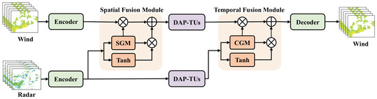
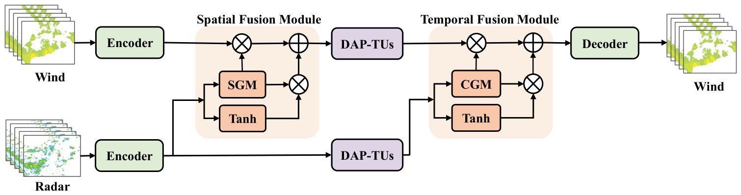
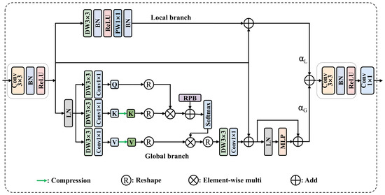
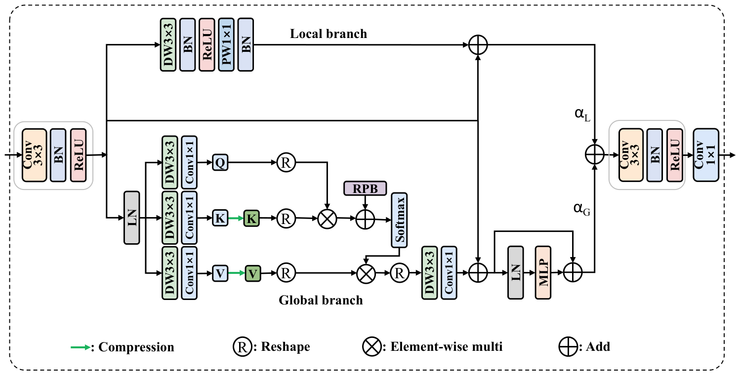
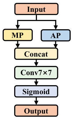
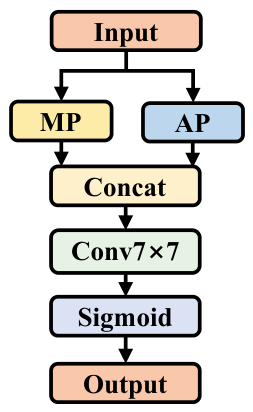
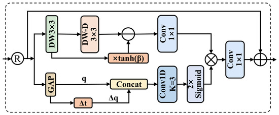
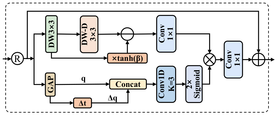
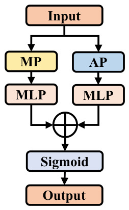
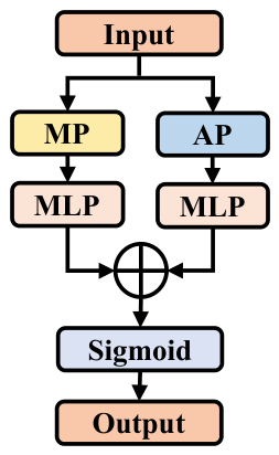
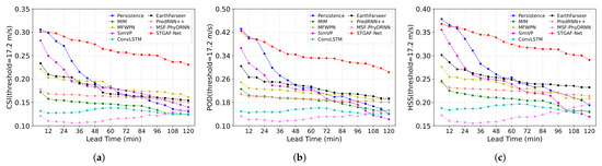
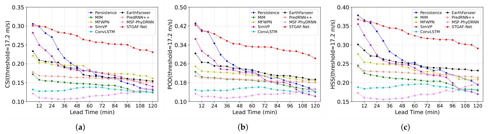
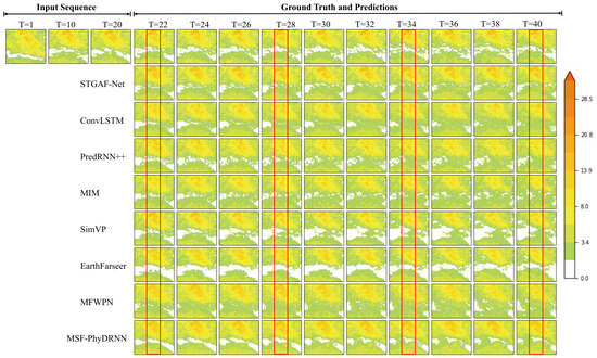
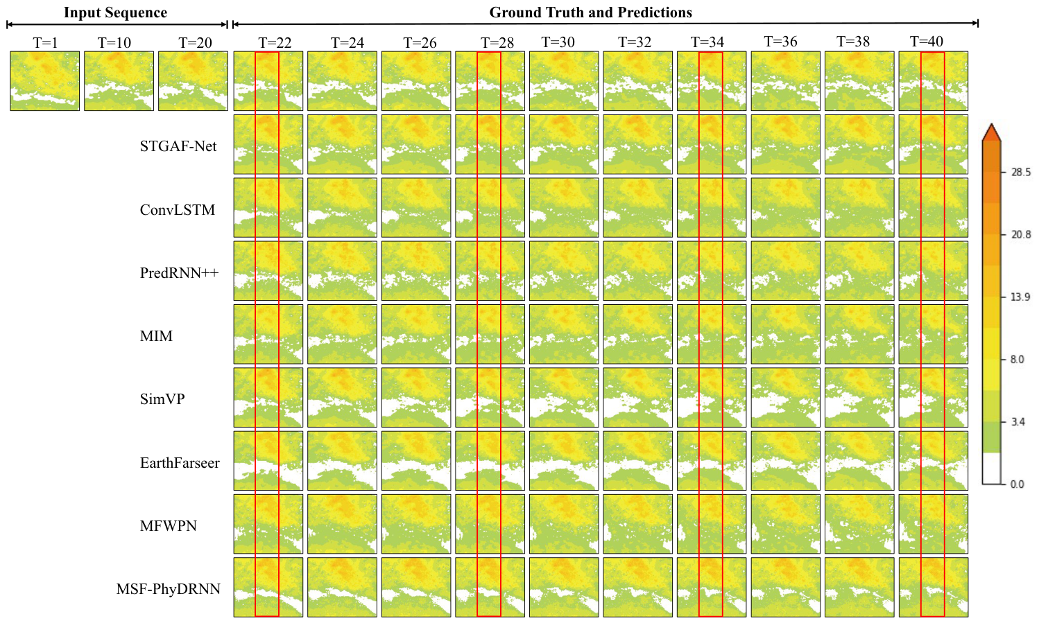
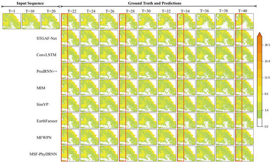
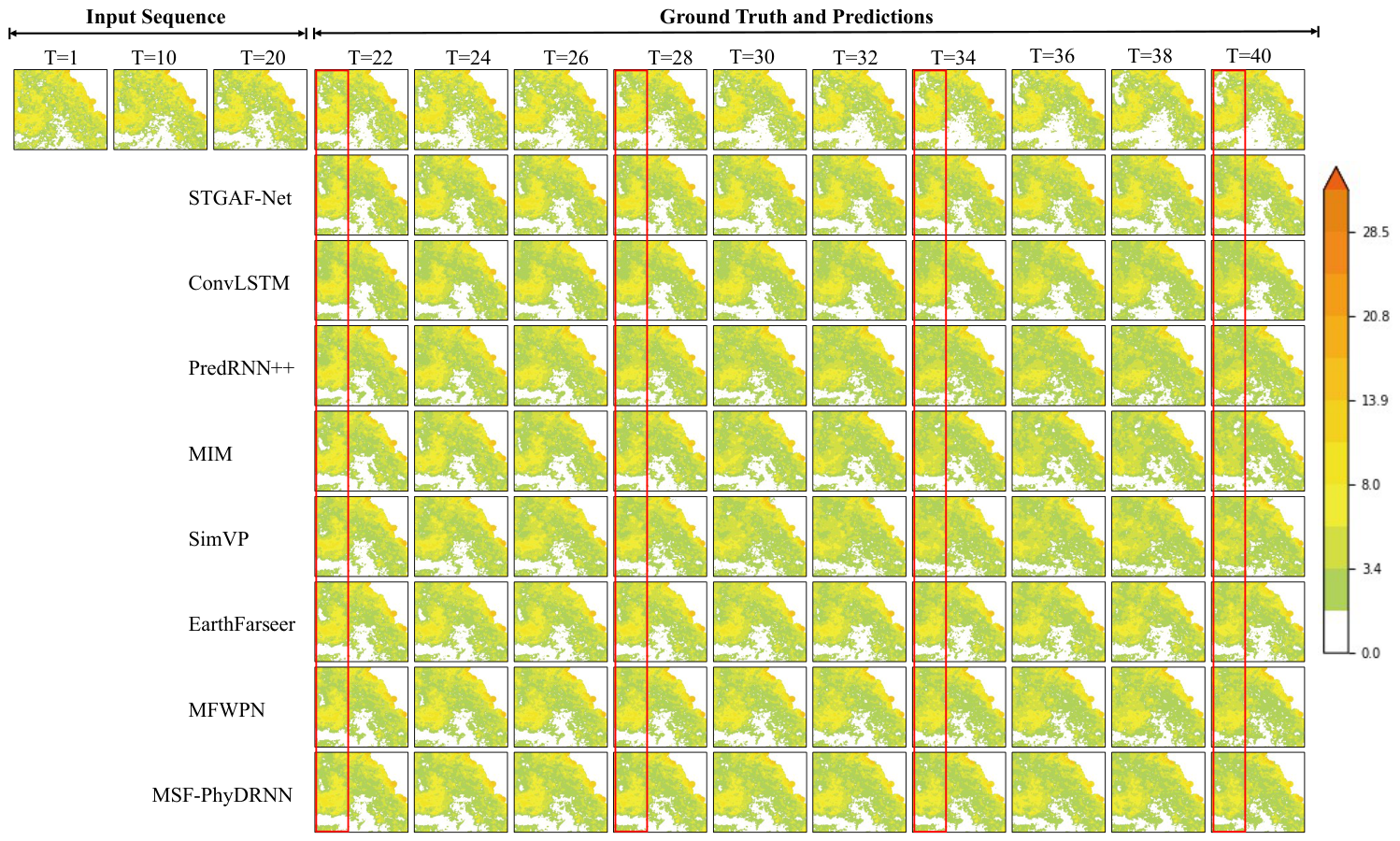
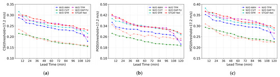
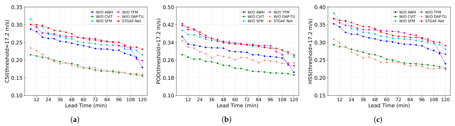
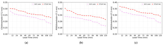
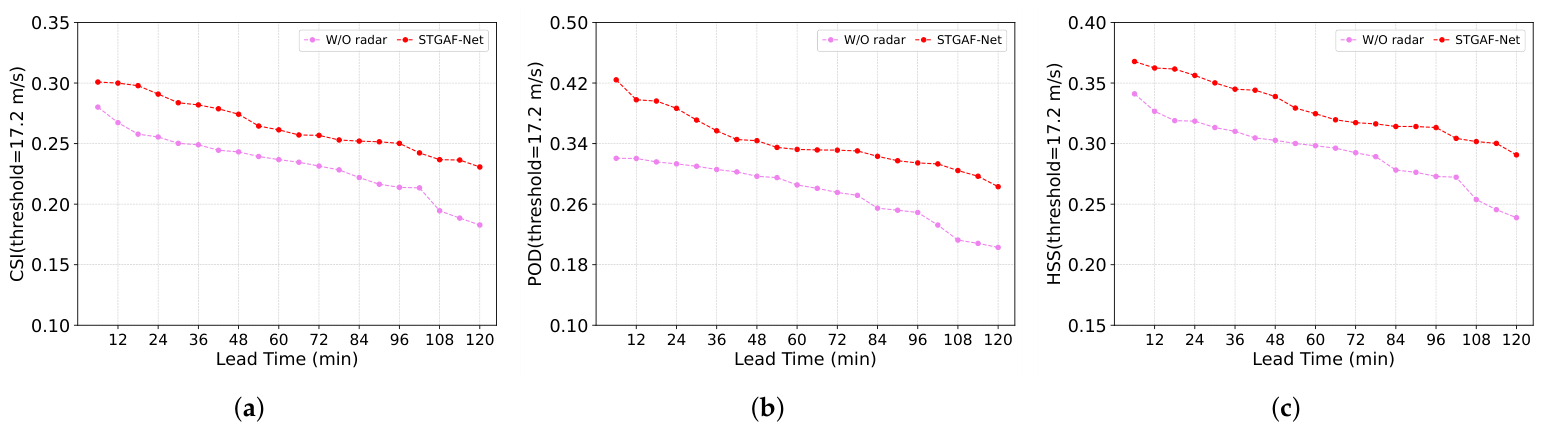

Disclaimer/Publisher’s Note: The statements, opinions and data contained in all publications are solely those of the individual author(s) and contributor(s) and not of MDPI and/or the editor(s). MDPI and/or the editor(s) disclaim responsibility for any injury to people or property resulting from any ideas, methods, instructions or products referred to in the content. |
© 2026 by the authors. Licensee MDPI, Basel, Switzerland. This article is an open access article distributed under the terms and conditions of the Creative Commons Attribution (CC BY) license.