


Highlights
What are the main findings?
- A phenological synchronization and time–frequency feature selection (FSITF) framework maps apple orchards with >93% overall accuracy and Kappa > 0.85 in Shandong and Shaanxi.
- Cross-year phenological alignment combined with harmonic time–frequency features effectively distinguishes spectrally and phenologically similar deciduous orchards.
What are the implications of the main findings?
- FSITF offers a re-applicable framework for large-scale, multi-year mapping of perennial orchards across heterogeneous regions.
- The framework supports regional orchard inventory, yield estimation, and grain–fruit land-use planning.
Abstract
Accurate spatial mapping of apple orchards is essential for regional agricultural planning and sustainable management; however, large-scale, multi-year mapping remains challenging because spectral confusion and climate-driven inter-annual phenological variation complicate interpretation. To address these challenges, we propose a Phenological Synchronization and Time–Frequency Feature Selection framework (FSITF) for high-precision apple orchard identification using Sentinel-2 time-series observations. We evaluated the framework in Shandong and Shaanxi provinces, two major apple-producing regions in China. FSITF consists of three main components: phenological synchronization, time–frequency feature construction, and discriminative feature selection. First, we develop a phenological synchronization strategy based on derivative analysis and correlation-based temporal alignment to reduce inter-annual and regional temporal discrepancies in phenological trajectories, thereby generating standardized cross-year phenological trajectories. Second, Harmonic Analysis is combined with temporal phenological metrics to construct a complementary time–frequency feature representation, enabling the characterization of complex perennial growth dynamics from both temporal evolution and periodic variation perspectives. Third, a dual-metric feature selection strategy integrating Jeffries–Matusita distance-based class separability and Random Forest-based feature importance is developed to identify informative features and reduce high-dimensional redundancy. Experimental results demonstrate that FSITF achieves overall accuracies exceeding 93% and Kappa coefficients above 0.85 in both study regions, outperforming conventional approaches without phenological synchronization and feature optimization. These results indicate that integrating phenological alignment, time–frequency feature representation, and orchard-oriented feature selection can effectively improve the accuracy and robustness of regional perennial crop mapping, providing a reliable framework for large-scale orchard monitoring.
1. Introduction
The apple (Malus domestica) is one of the most economically important temperate fruit crops worldwide. In 2023, global apple production reached approximately 89 million tonnes, with China contributing more than half of the total output. The Bohai Bay and Loess Plateau regions represent the dominant production areas, accounting for approximately 90% of China’s domestic apple production [1,2,3,4]. However, current orchard inventories mainly rely on statistical surveys and administrative records, which provide limited spatial information required for precision agricultural management. Accurate apple orchard mapping is therefore essential for agricultural planning, climate-risk assessment, and sustainable land-use management, particularly for balancing orchard development and grain-production conservation strategies [1,5].
Remote sensing has become a fundamental approach for large-scale crop and orchard mapping due to its ability to provide spatially continuous and repeated observations. Early studies mainly relied on spectral indices and single-date imagery, but these approaches were often limited by spectral similarity among vegetation types and seasonal variations. With the increasing availability of satellite time-series data, crop identification has gradually shifted toward phenology-based approaches that exploit temporal growth characteristics [6,7,8]. Sentinel-2 imagery, with 10 m spatial resolution and red-edge bands, has further improved vegetation monitoring and crop discrimination capability [9]. Meanwhile, multi-source data fusion, such as Sentinel-1 and Sentinel-2 integration, has enhanced classification robustness by combining spectral and structural information [10,11,12].
Along with advances in remote sensing data, crop mapping approaches have evolved from traditional machine learning to deep learning methods. Random Forest (RF) and Support Vector Machine (SVM) have been widely applied due to their strong nonlinear modeling capability and effectiveness under limited training samples [13,14]. However, these approaches rely heavily on manually designed spectral, vegetation-index, and phenological features, limiting their transferability across heterogeneous agricultural landscapes. Recently, deep learning methods, such as CNNs and Transformer-based architectures, have demonstrated strong capabilities in automatically extracting spatial and temporal representations from remote sensing data [15,16,17,18]. Nevertheless, their dependence on large amounts of labeled data, limited interpretability, and reduced cross-regional generalization remain important challenges [19,20].
Compared with annual crops, orchard mapping remains more challenging due to fragmented spatial distributions, complex canopy structures, and subtle phenological variations. Orchard landscapes often exhibit high intra-class variability and inter-class spectral similarity, resulting in “same object, different spectra” and “different objects, same spectra” problems in single-date observations [21,22,23,24]. Therefore, temporal information describing crop-specific growth trajectories has become increasingly important for reliable orchard identification.
Dynamic Time Warping (DTW) and Time-weighted Dynamic Time Warping (TWDTW) have been introduced into agricultural remote sensing to align satellite time series and reduce temporal inconsistencies in crop mapping [25,26,27]. However, these approaches mainly focus on correcting temporal displacement and cannot fully address nonlinear phenological variations caused by climatic fluctuations, cultivar differences, and agricultural management practices. For perennial crops such as apple, phenological trajectories may vary not only in timing but also in growth intensity across years and regions, limiting the robustness of conventional temporal alignment methods for cross-year and cross-regional mapping [28]. Unlike TWDTW, which performs pointwise nonlinear warping as a similarity measure for matching reference profiles, the proposed framework adopts a global temporal-shift strategy and further integrates time–frequency feature construction and feature selection. Therefore, beyond temporal alignment, a phenological synchronization strategy that also accounts for growth-intensity differences is required to establish consistent growth trajectories under complex environmental variations.
Although phenological synchronization can improve temporal consistency, it does not fully exploit the intrinsic growth rhythms embedded in vegetation time series. To further characterize complex perennial growth dynamics, time–frequency analysis provides an alternative perspective by simultaneously describing temporal evolution and periodic variation. Harmonic analysis extracts vegetation periodic characteristics through parameters such as amplitude and phase [29]. However, existing studies generally treat temporal and frequency-domain characteristics as independent information sources, and their complementary relationship remains insufficiently explored for perennial orchard identification. Furthermore, integrating multi-temporal and frequency-domain variables inevitably increases feature dimensionality and redundancy. Although feature selection methods based on statistical separability, machine-learning importance ranking, and optimization algorithms have been widely applied [30,31,32,33], most were developed for general crop classification and do not explicitly consider the spectral convergence and spatial heterogeneity of orchard environments. To address these challenges, this study proposes a Phenological Synchronization and Time–Frequency Feature Selection framework (FSITF) for high-resolution apple orchard mapping using Sentinel-2 time-series observations. The main contributions are summarized as follows:
(1) A phenological synchronization mechanism is developed to improve the temporal consistency of apple growth trajectories across years and regions.
(2) A time–frequency feature representation strategy is proposed to integrate phenological evolution and periodic growth characteristics for enhanced orchard identification.
(3) A dual-metric feature selection strategy combining Jeffries–Matusita distance and Random Forest importance is introduced to reduce feature redundancy and improve mapping robustness.
2. Materials
2.1. Study Area
This study evaluates the proposed method across Shaanxi and Shandong, which represent the two leading apple-producing provinces in China (Figure 1). Shaanxi (31°42′–39°35′N, 105°29′–111°15′E) serves as the top producer, with 1.168 million hectares of orchards as of 2023. Its diverse topography, ranging from northern plateaus to southern mountains, and varied climate zones spanning from subtropical to warm temperate provide ideal conditions for apple cultivation. The annual precipitation ranges from 500 to 700 mm, and the accumulated temperature above 10 °C varies between 3000 and 4500 °C. Shandong (34°23′–38°17′N, 114°48′–122°42′E), the second-largest producer, maintains 236,500 hectares of apple orchards primarily concentrated in the Jiaodong Hills. The region’s cool climate, significant diurnal temperature variations, and loose, permeable sandy loam soil meet the physiological requirements of apple trees, with an annual precipitation of approximately 600–800 mm and accumulated temperature above 10 °C of 3500–4500 °C. The distinct longitudinal and latitudinal gradients between these two provinces result in significant phenological shifts, making them ideal for validating the robustness of the FSITF framework in cross-regional orchard mapping.
Figure 1.
Location of the study areas and distribution of ground-truth samples. (a) Location of the study area within China; (b) Shaanxi Province; (c) Shandong Province.
2.2. Datasets
2.2.1. Data Sources and Preprocessing
Sentinel-2 optical imagery from the European Space Agency (ESA) Copernicus program was used in this study. The Sentinel-2A/B constellation provides a 5-day revisit frequency and includes three red-edge bands, making them particularly useful for vegetation monitoring and crop classification [34,35]. Sentinel-2 Level-2A Surface Reflectance (SR) products, atmospherically corrected using the Sen2Cor algorithm [36], were obtained from the Google Earth Engine (GEE) platform for the period from January 2022 to December 2024, with 2651, 2826, and 2782 scenes in 2022, 2023, and 2024, respectively. Clouds, cloud shadows, cirrus, and saturated/defective pixels were removed using the Scene Classification Layer (SCL), and images with a cloudy-pixel percentage below 70% were retained. After cloud masking, each pixel had on average 62, 68, and 63 valid observations in 2022, 2023, and 2024, respectively. A stricter 30% cloudy-pixel threshold was applied for harmonic fitting.
Sentinel-1 synthetic aperture radar (SAR) data were also incorporated to provide complementary observations under cloudy conditions. Three time series were derived from Sentinel-1 data: VV backscatter, VH backscatter, and the VH/VV backscatter ratio, to characterize variations in canopy structure and moisture conditions. Sentinel-1A Level-1 Ground Range Detected (GRD) products acquired in 2023 were obtained from GEE. The selected data were acquired in Interferometric Wide (IW) swath mode with dual VV and VH polarization, using ascending orbits with relative orbit numbers 40, 69, 98, 142, and 171, and comprised 439 scenes. The GRD products had undergone radiometric calibration and terrain correction as part of the product processing. GRD data were used instead of Single Look Complex (SLC) data because this study focused on backscatter intensity rather than phase information.
2.2.2. Field Investigation Data
Field surveys were conducted in major fruit-growing regions of Shandong Province (SD), covering apple orchards and other horticultural crops, including peach, cherry, and grape (Figure 1). In 2022, a total of 269 orchard parcels were surveyed, while 248 cropland and forest parcels were identified through visual interpretation of high-resolution Google Earth imagery. These samples were further validated using multi-temporal Google Earth imagery from 2022 to 2024, and 158 parcels with stable apple cultivation were retained. Based on these verified locations, sample augmentation through visual interpretation generated 969 apple samples and 1717 non-apple samples (Table 1).
Table 1.
Overview of field-surveyed crop samples in the study areas.
In Shaanxi Province (SX), field surveys targeted major apple-producing regions and commercial orchards. Between 2024 and 2025, 377 stable apple parcels and 85 parcels of other horticultural crops were identified through field surveys, while 359 cropland and forest parcels were delineated through visual interpretation of Google Earth imagery. All parcels were further checked against multi-temporal Google Earth imagery from 2022 to 2024 to ensure that only orchards with stable cultivation throughout the study period were retained. Using the same sample augmentation strategy as in Shandong Province, 2261 apple samples and 2140 non-apple samples were generated (Table 1). The surveyed apple orchards in both Shandong and Shaanxi provinces were dominated by the Fuji cultivar group, which is the predominant commercial apple group in China and accounts for a substantial proportion of apple production in both regions. Consequently, the ground-truth samples primarily represent the Fuji cultivar group, and the transferability of the resulting models to other cultivars, particularly those with distinct fruit colors, warrants further investigation.
To ensure label accuracy despite the high spectral, textural, and phenological similarities among deciduous fruit orchards, multi-source visual reference keys were established using high-resolution Google Earth imagery and ground-level photos (Figure 2). While medium-resolution satellite imagery presents homogeneous textures across these orchards, high-resolution Google Earth imagery captures spatial row arrangements (Figure 2a–c), and ground photos reveal subtle differences in branching architecture (Figure 2d–f). Integrating these fine-scale structural features guarantees high ground-truth purity for algorithm development and evaluation.
Figure 2.
Multi-source visual reference keys for distinguishing spectrally and texturally similar deciduous fruit orchards. Top row: High-resolution Google Earth imagery capturing spatial row arrangements and textures of (a) apple, (b) peach, and (c) pear orchards. Bottom row: Corresponding ground-level field photos illustrating tree canopy architectures and branching habits of (d) apple, (e) peach, and (f) pear trees.
2.2.3. Statistical Data for Validation
To evaluate the spatial reliability of the derived apple acreage products, statistical data from the National Bureau of Statistics (NBS) of China were used as reference data. The estimated apple acreage derived from the proposed FSITF framework was compared with officially reported statistics at corresponding administrative levels.
3. Methods
3.1. Overview of the FSITF Algorithm
The proposed algorithm for apple orchard mapping comprises four primary components, as illustrated in Figure 3. First, recognizing that orchards exhibit significant spatiotemporal stability, they are inherently suited for multi-year, multi-temporal image synthesis. The first component develops a pixel-level spectral feature enhancement method through the alignment and synthesis of samples from stable parcels across a three-year period [37]. This approach generates enhanced and stabilized spectra temporal sequences while simultaneously minimizing computational overhead.
Figure 3.
Overall workflow of the FSITF method.
The second component employs harmonic analysis (HA) to characterize Sentinel-2 NDVI and textural index time series [38]. Harmonic parameters derived from these time series are incorporated as phenological features to enhance the model’s discriminatory power. The third component incorporates Sentinel-1 polarization features to capture structural and moisture-related characteristics of apple orchards, which typically exhibit more regular planting patterns and distinct canopy structures and water conditions than other forest types. Harmonic regression is further applied to the VV, VH, and VH/VV ratio time series to extract complementary seasonal information from SAR observations. Unlike optical indices, which are analyzed within specific phenological windows, SAR backscatter is affected by speckle noise and does not necessarily exhibit consistent directional changes within these windows. Therefore, harmonic regression is applied to the full-year SAR time series to characterize low-frequency seasonal variations while mitigating the influence of high-frequency fluctuations, thereby providing a complementary temporal representation to the optical features. However, integrating these diverse data sources substantially increases the dimensionality of the feature space, potentially compromising model performance and computational efficiency. To address this issue, the fourth component integrates the outputs of the three preceding components into a feature selection framework that identifies the most informative variables and constructs an optimized feature set for orchard mapping.
3.2. Automated Phenological Extraction and Cross-Year Alignment Module
3.2.1. Automated Identification of Phenological Stages
To overcome the issue of temporal discontinuity in single-year sequences caused by cloud interference, this study proposes a phenological feature enhancement and automated identification scheme tailored to the spatiotemporal stability of orchards.
Because apple trees are perennial woody plants with relatively stable spatial distributions, this study used a three-year synthesis approach based on the target year and its adjacent years (2022, 2023, and 2024). The initial NDVI time series were derived from median-composited Sentinel-2 imagery using Google Earth Engine (GEE). The three-year NDVI time series were then interpolated at 10-day intervals and smoothed using a Savitzky–Golay (SG) filter with a window length of 7 and a second-order polynomial (polyorder = 2) (Figure 4). These settings were chosen to reduce noise from clouds and atmospheric effects while preserving the rapid increases and decreases in the orchard NDVI curves during green-up and senescence. This helped avoid false turning points caused by insufficient smoothing and the loss of real turning points caused by excessive smoothing. By combining pixel-level spectral information from three consecutive years, this method reduced random noise caused by cloud contamination and produced a stable three-year reference curve that better represents vegetation growth patterns.
Figure 4.
NDVI temporal trajectories of apple samples in Shandong (SD) and Shaanxi (SX) after interpolation and smoothing.
Upon obtaining the reconstructed NDVI sequences, an inflection point detection algorithm based on mathematical derivative analysis was designed and implemented to facilitate the automated segmentation of phenological stages. The algorithm first computes the derivative of NDVI with respect to time using numerical differentiation to characterize the vegetation growth rate. By searching for derivative extrema within predefined physiological time windows, the inflection points of the curves are precisely localized. Compared to traditional methods relying on human-defined thresholds, this algorithm achieves objective identification of critical transition points in growth status by capturing the intrinsic geometric variations of the temporal profiles.
Based on the inflection point detection results, the algorithm automatically extracts the following key phenological parameters and their corresponding growth stages. The modeling process is illustrated in Figure 5a. Specifically, let the smoothed NDVI sequence over one year be denoted as , where represents DOY, and its finite difference approximate derivative is
Figure 5.
A Spatiotemporal Collaborative Alignment Method Based on Correlation Analysis. (a) Derivative-based inflection-point detection, in which the smoothed NDVI curve and its derivative are used to locate the green-up, plateau-start, and decline-start turning points that divide the growing season into the dormancy, growth, plateau, and decline stages. (b) Correlation-based multi-year alignment, in which the reference-year (2023) NDVI profile is matched against each target-year profile within a sliding window by maximizing the Pearson correlation coefficient to estimate the optimal lag and align the phenological stages across years.
Record the annual peak value and peak time as:
The algorithm sequentially determines three critical turning points: green-up, plateau start, and decline start.
Green-up: Within the ‘NDVI rising segment’ , locate the point of maximum growth rate:
If the detected deviates from the actual physiological time window (DOY < 125), re-select the maximum point of within this window as the corrected ; plateau start: Set the peak growth rate [39]:
Plateau start: Define as follows:
where .
Decline start: Since decline occurs after the peak, the search interval is . If the interval since the peak period meets , and NDVI declines below of the peak value, with the proportion of negative derivatives in the length time window not less than , define:
where , , , . If the above set is empty, the fallback criterion applies:
Here, the physical meaning and setting of these thresholds are as follows. For plateau onset (Equation (5)), requires the growth rate to fall below 10% of its peak value, marking the end of the rapid green-up phase, and requires the NDVI to remain above 60% of the annual maximum, ensuring that the canopy has not yet entered senescence. For decline onset (Equation (6)), identifies the point at which NDVI falls below 95% of the peak value, days imposes a minimum interval after plateau onset to prevent short-term fluctuations from being misidentified as the true decline, and the condition that at least of the derivatives in a point window are negative confirms a sustained decline rather than a single-day drop.
Ultimately, the complete growing season is partitioned into four distinct phenological stages: dormancy, growth, plateau, and decline:
The phenological metrics derived from Equations (1)–(7) follow the widely recognized threshold- and derivative-based logic for satellite time-series analysis [40]. The dynamic thresholds and window sizes were configured as empirical parameters, optimized according to the seasonal NDVI curves of orchard samples in the study area. The identified green-up, plateau-start, and decline-start dates were consistent across the three years and the two study regions (Figure 4), indicating that the detected phenological transitions were stable under the selected smoothing parameters.
This methodology integrates the overall dynamic characteristics of the NDVI profile while incorporating rate-of-change analysis and threshold constraints. By doing so, it effectively mitigates the issues of unreliability and lack of interpretability associated with the manual determination of phenological periods in previous studies [37]. Consequently, this approach establishes a robust foundation for subsequent phenology-based feature extraction and classification.
3.2.2. Multi-Year Phenological Standardization and Alignment
However, inherent variations in climatic conditions and phenological responses across different years can lead to temporal misalignments when directly merging annual phenological segments. This misalignment adversely affects subsequent feature extraction and cross-year comparative analysis. To address this issue, building upon the methodology of Sun et al., this study developed a spatiotemporal synergistic alignment method based on correlation analysis (Figure 5b) [41]. The core strategy involves designating the target year as the reference year; the smoothed NDVI curve and its corresponding phenological stages for the reference year are first extracted. Subsequently, Pearson’s correlation coefficient (PCC) is utilized within a sliding window to calculate the similarity between the profiles of other years and the reference year [42,43]. The optimal temporal offset was determined to quantify and correct differences in phenological timing between years. The NDVI time series were reconstructed at 10-day intervals, with 2023 used as the reference year. For the cross-year validation described in Section 4.6.1, 2024 was used as the reference year instead. The lag search range was defined as ±30 days to capture possible inter-annual phenological shifts caused by climatic variability.
This coefficient was selected because, during the green-up phase, NDVI values exhibit a strong linear correlation with time, rendering PCC particularly suitable for this application. Moreover, PCC offers the advantages of computational efficiency, high interpretability, and robust stability across large datasets. While existing studies have predominantly employed PCC for extracting experimental metrics or quantifying experimental results, its integration as a mechanism for index sequence alignment within a mapping framework remains significantly under-explored [44,45,46].
Specifically, using the NDVI sequence from reference year as the baseline, the sequence for target year is denoted as . Within the critical growth season window , the optimal lag length is estimated by maximizing the PCC, defined as:
Here, corr denotes the PCC calculated at valid overlapping sampling points. After obtaining , the phenological stages of the reference year are projected onto the target year using a global shift: . This process completes the overall shift of the reference year’s phenological stages by the lag value, yielding projected phenological stages for subsequent years. This ensures temporal consistency of phenological phases across the three-year period. This approach mitigates climate-induced phenological shifts while preserving cross-year comparability for subsequent feature extraction and classification. Finally, the aligned phenological periods are synthesized to produce a more robust three-year composite image.
3.3. Integration of Multi-Source Time-Domain and Frequency-Domain Features
3.3.1. Time-Domain Feature Extraction
Time-domain features aim to capture the fundamental biophysical properties of vegetation growth by characterizing the geometric morphology and mathematical distribution of NDVI over time. Building upon the critical phenological nodes identified in Section 3.2, this study first extracted a suite of phenological parameters, including the length of the growing season, the date of peak greenness, and the green-up slope. To quantify the annual vegetation coverage fluctuations, we performed statistical modeling on the raw NDVI time series, calculating its mean, standard deviation, skewness, and kurtosis. Furthermore, to capture spatial structural characteristics, the NDVI data were normalized and rescaled to a grayscale range; subsequently, four categories of textural features-Angular Second Moment, Contrast, Correlation, and Entropy-were extracted using the Gray-Level Co-occurrence Matrix (GLCM). These time-domain metrics, derived from the original temporal dimension, provide essential background information for discriminating orchards from open-field crops.
3.3.2. Frequency-Domain Feature Extraction
Frequency-domain analysis enables the decomposition of complex time-series signals into oscillation patterns across various frequencies. Specifically, HA is employed to extract the inherent periodic growth signatures of vegetation. Given that the inter-annual variability of vegetation indices exhibits mathematical properties analogous to Fourier series decomposition, the essence of HA lies in performing a finite-order Fourier expansion on the time series. Its general form can be expressed as
In this formulation, denotes the baseline component, representing the overall vegetation level throughout the year. The terms and are the th-order Fourier coefficients corresponding to the sine and cosine components, respectively, while represents the residual error. By performing secondary transformations on , a suite of more intuitive harmonic-derived parameters can be obtained as follows:
(1) Amplitude (): This parameter characterises the intensity of the periodic fluctuation of the order and reflects the degree of fluctuation within the intra-annual vegetation dynamics. It is expressed as:
(2) Phase (): It reflects the temporal offset of the order periodic component along the timeline, thereby revealing the advancement or lag in the start of season (SOS) or peak growth timing. It is expressed as:
(3) Baseline (): It describes the overall annual mean level of the vegetation index, reflecting the background biomass intensity throughout the year.
High-order fluctuation intensity (): This metric integrates the amplitudes of the second and third harmonics to characterize more complex intra-annual oscillations or double-peak phenomena. It is particularly effective for interpreting the growth patterns of perennial fruit trees or crops with multiple growth peaks [47]. It is expressed as:
Specifically, while the first harmonic () captures the macro-annual single-peak growth trend, higher-order harmonics ( and ) are sensitive to intra-annual sub-seasonal fluctuations, such as rapid spring green-up, canopy management, and ground-cover dynamics beneath the orchard canopy. Integrating and into Afluc effectively characterizes complex perennial canopy oscillations, differentiating orchards from single-peak forests and double-peak cropland.
(5) Fitted peak (): It represents the theoretical maximum value of the harmonic-reconstructed curve throughout the year, reflecting the idealized peak productivity of the vegetation.
3.3.3. Feature Integration and Fusion Strategy
This study adopts an early fusion strategy directly concatenating temporal phenology, spatial texture, and frequency-domain harmonic features prior to model input, thereby maximizing the exploration of non-linear coupling among these ‘spatial-temporal-frequency’ dimensions and preventing the information loss inherent in the independent modeling of late fusion.
Specifically, this study integrated NDVI time series and four categories of GLCM textural sequences into the HA model for third-order Fourier expansion. This joint approach captures the periodic patterns of spatial textures as they evolve alongside phenological succession. While HA has been successfully applied to crop classification and intensity detection [47,48,49], its efficacy in discriminating fruit tree species, particularly for apple orchard mapping, remains under-explored. This study subsequently validates the distinct advantages of HA for robust orchard identification.
3.4. Construction of the Optimal Discriminative Feature Subset
3.4.1. Automated Feature Optimization and Selection Module
Following the cross-annual phenological alignment, an initial screening of optical spectral indices was conducted within the unified phenological time windows. For the Sentinel-2 imagery, a comprehensive suite of candidate features was constructed, encompassing spectral vegetation indices, red-edge indices, photochemical sensitivity indices, and soil moisture indices (Table 2). These indices capture key physiological and biochemical attributes of vegetation, including chlorophyll content, canopy structure, water stress, and senescence signals, thereby providing a holistic representation of the spectral discrepancies between fruit trees and other land cover types across distinct growth stages.
For each index within every phenological stage, the JM distance was first calculated between apple orchard and non-apple samples to quantify the class separability [50,51]. The JM distance is mathematically defined as:
where and represent the mean and variance calculated for apple and non-apple samples, respectively. A larger JM distance signifies a stronger separability between these two categories for a given index. However, as JM distance is based solely on the mathematical statistics of class means and variances, it fails to account for the non-linear contributions or complex inter-feature interactions during the actual classification process. To address this limitation, RF Feature Importance () was introduced to evaluate the empirical contribution of each index within the classification model, thereby enhancing the robustness and practicality of the feature selection process. For the set of indices within each phenological stage, an RF classifier was trained using the sample points:
thereby extracting the Feature Importance for each index. Finally, for every individual index, the distance and values are normalized, and a comprehensive score is calculated according to the following formula
where X denotes the index under evaluation; and represent the normalized JM distance and Feature Importance, respectively. is the comprehensive score for the index, and signifies the weight assigned to the JM distance within the scoring framework, which is set to 0.6 in this study. Because the JM distance directly measures class separability and serves as the primary screening criterion, it was assigned a higher weight (α = 0.6) than RF importance, which complements the JM distance by accounting for feature importance within the model. A sensitivity analysis with α values ranging from 0.3 to 0.8 showed that the feature rankings remained stable across all tested settings. Specifically, ratio_A0 remained the top-ranked Sentinel-1 harmonic feature, NDVI_A0 remained the top-ranked Sentinel-2 harmonic feature, and PSRI and NDWI remained the leading spectral indices across the growth, plateau, and decline stages. These results indicate that the feature selection results were robust to changes in the weighting parameter (Figure 6). Subsequently, the extracted harmonic phenological features are processed through the same framework for feature selection and optimization.
Figure 6.
Sensitivity of the comprehensive-score ranking to the JM–RF weighting parameter α. The comprehensive scores of the top candidate features are shown as α varies from 0.3 to 0.8 for (a) Sentinel-1 harmonic features, (b) Sentinel-2 harmonic features, and the spectral indices in the (c) dormancy, (d) growth, (e) plateau, and (f) decline stages.
Table 2.
Candidate spectral indices.
3.4.2. Multi-Criteria Feature Selection
To identify the optimal feature combination, a multi-criteria selection strategy was implemented. First, the Recursive Feature Elimination algorithm was employed to effectively capture inter-feature interactions by iteratively constructing RF models and removing variables with the smallest contribution weights. This process ensures the retention of core variables that contribute most significantly to reducing classification error. Subsequently, drawing on the principle of Forward Selection, auxiliary features were introduced one by one based on a baseline of key phenological features with high JM distance and RF importance scores. This incremental evaluation ensured that each newly selected feature provided a positive gain to the OA. Ultimately, an efficient feature subset was constructed, capable of robustly addressing the complex spatial heterogeneity of apple orchards.
3.4.3. Determination of the Optimal Feature Subset
The selection of the final feature combination aims to achieve an optimal balance between classification accuracy and computational efficiency. This study employed a cross-validation approach to assess the robustness of candidate feature subsets across various scales. By calculating the OA and Kappa coefficient for each subset, the relationship between accuracy increments and the increasing number of features was quantitatively analyzed [61]. Building on this, a dimensionality-accuracy trade-off analysis was conducted to identify the saturation point where further accuracy gains became negligible. The feature combination at this point, which is characterized by minimum dimensionality and peak performance, was selected as the final subset.
3.5. Classifier Design and Hyperparameter Optimization
3.5.1. RF Classifier
The Random Forest (RF) classifier was employed as the core classifier for apple orchard mapping due to its effectiveness in handling complex remote sensing features. RF generates classification results by integrating multiple decision trees through a voting mechanism. In this study, the RF model was trained using the extracted feature set, with the number of decision trees () set to 200 and the random seed fixed at 42. The number of features considered for splitting each node (max_features) was set to 3. The dataset was randomly divided into training and validation sets at a ratio of 70% and 30%, respectively. Feature selection was conducted on the training set, while the reported accuracies were evaluated on the independent validation set, thereby avoiding optimistic estimates caused by using the same samples for both feature selection and accuracy assessment.
3.5.2. Ensemble Learning Strategy
To reduce the influence of class imbalance between apple orchards and non-apple areas, stratified random sampling was applied to maintain the proportional representation of different classes in the training and validation datasets. Because the sample points were geographically dispersed across the two study regions and no spatial blocking was imposed, training and validation samples drawn from nearby parcels may be spatially autocorrelated, which could lead to slightly optimistic accuracy estimates. The voting mechanism of multiple decision trees improved classification stability in complex boundary areas.
3.6. Evaluation Metrics
Classification performance was evaluated using five metrics derived from the confusion matrix, including overall accuracy (OA), the Kappa coefficient, producer’s accuracy (PA), user’s accuracy (UA), and the macro-averaged F1-score. The agreement between estimated apple acreage and the statistics reported by the National Bureau of Statistics (NBS) was assessed using the coefficient of determination (R2) and the root mean square error (RMSE). These metrics are summarized in Table 3, where TP, TN, FP, and FN denote true positives, true negatives, false positives, and false negatives; is the expected agreement by chance; and are the reported and estimated acreages, respectively; is the mean reported acreage; and n is the number of administrative units.
Table 3.
Evaluation metrics used in this study.
4. Results
4.1. Establishment and Alignment of Key Phenological Stages
As shown in Figure 4, Shaanxi Province exhibits lower overall NDVI values and greater intra-annual variability than Shandong Province, where NDVI profiles are more consistent. These differences may be related to the development of orchard landscapes in the two regions. The recent expansion of apple-growing areas in Shaanxi has resulted in orchards of different ages and ongoing tree planting, leading to greater variation in canopy density. In contrast, Shandong is a traditional apple-producing region where most orchards have reached the mature, full-bearing stage and developed relatively high canopy cover. Despite these differences in NDVI magnitude, the phenological patterns are broadly consistent between the two regions, and the timing of key growth stages agrees with the results presented in Section 3.2.1.
Taking 2022 as an example, the algorithm identified three key phenological dates in Shandong Province at DOY 111, 161, and 251, corresponding to the green-up, plateau-start, and decline-start dates, respectively. In Shaanxi Province, the corresponding dates were DOY 121, 151, and 251. Based on the phenological stages identified in both regions, the final key periods for apple orchards were defined as dormancy [1, 111), growth [121, 151), plateau [161, 251), and decline [251, 366).
Interannual variations in climate and precipitation can lead to corresponding changes in apple growth patterns. Figure 7 illustrates the shifts in NDVI growth curves across different years, with the highlighted gap representing the interannual phenological offset, or the difference in the timing of apple growth transitions between years. Meanwhile, Figure 4 shows a relatively consistent linear increase in NDVI around DOY 100, providing a suitable reference interval for the phenological alignment method described in Section 3.2.2. Accordingly, the alignment window was set to [80, 140], and the temporal lag between each year and the reference year was then determined.
Figure 7.
Interannual lag discrepancies among the three-year time-series curves.
Furthermore, a comparative analysis between apple orchards and other fruit crops (Figure 8) reveals a striking similarity among various deciduous fruit trees. Apple, cherry, and peach orchards exhibit high phenological synchronicity in their NDVI time series, with nearly identical waveform morphologies, peak positions, and critical phenological milestones. This results in severe inter-class overlap within the temporal statistical feature space, making it exceedingly difficult to isolate apple orchards using raw geometric characteristics alone. This ‘isospectral-isophenological’ phenomenon suggests that traditional classification methods, which rely on macro-growth rhythms, encounter a performance bottleneck when distinguishing similar woody perennials, thereby justifying the necessity of incorporating frequency-domain features and strategic feature selection.
Figure 8.
Smoothed NDVI time-series curves of different fruit tree species in 2023.
4.2. Comparison of PCC and DTW for Cross-Year Phenological Alignment
To further evaluate the proposed phenological synchronization method, Dynamic Time Warping (DTW) was used for comparison with the PCC-based alignment method. With 2023 as the reference year, both methods were applied to multi-year NDVI time series, and their performance was assessed using the correlation coefficient between NDVI trajectories. As shown in Table 4, the estimated phenological shifts differed among years. For 2022 and 2023, PCC identified a 10-day temporal shift and increased the correlation coefficient from 0.9279 to 0.9415 after alignment. In comparison, DTW achieved a correlation coefficient of 0.9268. For 2024 and 2023, PCC detected no temporal shift, and the correlation coefficient remained unchanged at 0.9690. DTW achieved a slightly higher correlation coefficient of 0.9818 through nonlinear temporal alignment. Although DTW achieved higher similarity in some cases, PCC-based alignment was more suitable for this study because it estimates an overall temporal shift while preserving the original shape of the phenological trajectory.
Table 4.
Comparison of PCC-based and DTW-based phenological alignment using multi-year NDVI trajectories.
4.3. Selection of Spectral–Temporal Features Within Phenological Windows
In this study, a synergistic feature selection strategy based on spectral separability and RF importance was implemented across four distinct phenological stages. Specifically, the JM distance and RF importance scores of each spectral index were calculated for both study areas and integrated into a comprehensive score for feature ranking (Figure 9). The comprehensive score was used to identify the most discriminative indices, while the top three indices from each region within the same phenological phase were combined to form the candidate feature pool. Subsequently, the statistical distributions of these candidate indices were evaluated using boxplots (Figure 10), and indices with greater separability between apple orchards and non-apple areas were retained. Finally, the definitive multi-temporal spectral index sets were determined as follows: Dormancy [PSRI, EVI], Growth [PSRI, NDWI], Plateau [PSRI, NDWI], and Decline [PSRI, NDWI, EVI].
Figure 9.
RF importance, JM distance, and integrated scores of spectral indices within different phenological stages in SD and SX.
Figure 10.
Statistical boxplots of the feature importance scores across different growth stages (Dormancy, Growth, Plateau, and Decline) under SD and SX periods: (a) Dormancy stage; (b) Growth stage; (c) Plateau stage; (d) Decline stage. (Note: The cross symbol ‘×’ indicates the mean value, the horizontal line inside the box represents the median, and ‘1.5*IQR’ denotes 1.5 times the interquartile range).
4.4. Frequency-Domain Features Derived from Fitted Phenological Curves
HA has been widely used in crop classification to extract frequency domain features that describe seasonal phenological patterns. Building on the temporal spectral indices selected in Section 4.3, this study further incorporated harmonic features into the feature selection framework. NDVI was selected as the only optical index for HA for two main reasons. First, NDVI time series generally show smooth and continuous seasonal patterns, making them suitable for Fourier analysis. In contrast, moisture-related indices, such as NDWI and LSWI, may show sharp local fluctuations that affect the quality of harmonic fitting. Second, applying HA to multiple vegetation indices would increase the number of features and the risk of multicollinearity. Therefore, combining NDVI-based harmonic features with phenological metrics derived from other vegetation indices helps represent seasonal patterns while controlling feature dimensionality. Specifically, HA was applied to Sentinel-2 NDVI time series, their associated texture metrics, and three Sentinel-1 polarization time series, namely VV, VH, and the VH/VV ratio, to extract frequency domain features. Following the feature screening procedure described above, the importance scores of individual features were calculated (Figure 9). The top four features from each study area were then combined to form a candidate feature set for further statistical evaluation (Figure 11). During the final feature selection stage, the harmonic features derived from Sentinel-2 NDVI and its associated texture metrics were examined. As shown in Figure 11, NDVI_A1 showed substantial overlap in the box plots and similar median values for apple and non-apple classes in both study areas, indicating limited ability to distinguish between the two classes. It was therefore excluded from the final feature set, while NDVI_A0, NDVI_A2, NDVI_A3, and NDVI_Afluc were retained. The candidate SAR feature set consisted of harmonic parameters derived from the VV, VH, and VH/VV ratio time series. Annual median backscatter features, including VV, VH, and VH/VV, were also evaluated but showed limited discriminatory ability and were therefore excluded from the final feature set. As shown in Figure 11, most Sentinel-1 harmonic features exhibited similar statistical distributions and limited separability between apple and non-apple classes. Among these features, ratio_A0 achieved the highest overall score in both study areas and showed sufficient class separability. It was therefore selected as the only Sentinel-1 harmonic feature retained in the final model. The final feature subset was formed by combining the top candidate features from both study regions, resulting in the same feature set for both regions and all three study years. It included the spectral indices PSRI, EVI, and NDWI, selected for their respective phenological stages, as well as five harmonic features, namely NDVI_A0, NDVI_A2, NDVI_A3, NDVI_Afluc, and ratio_A0.
Figure 11.
Statistical boxplots of the frequency-domain phenological feature sets, where is the composite score of the indices: (a) NDVI feature sets under SX and SD periods; (b) Ratio feature sets under SX and SD periods. (Note: The cross symbol ‘×’ indicates the mean value, the horizontal line inside the box represents the median, and ‘1.5*IQR’ denotes 1.5 times the interquartile range).
4.5. Feature Separability and Subset Optimization Based on JM Distance
After identifying the candidate feature set, the interclass separability of the selected features was quantitatively evaluated and optimized using the JM distance (Figure 12). The results show that adding features progressively improved the ability to distinguish apple orchards from spectrally similar land cover types. In particular, adding harmonic features, such as NDVI_A2, increased the JM distance between apple orchards and other confusing land cover types. These findings demonstrate the value of harmonic features in capturing seasonal growth patterns that help distinguish apple orchards from other land cover types.
Figure 12.
JM distance, RF importance, and comprehensive scores of harmonic features in SD (a) and SX (b).
The ablation experiments (Table 5 and Table 6) further demonstrate the effectiveness of the feature selection method. Combining JM distance with RF feature importance helped remove redundant features and reduce computational costs. Despite the substantial reduction in feature dimensionality, the selected feature set maintained high classification accuracy in both study regions. However, direct transfer of the model between the two regions remained limited, as discussed in Section 5.4.
Table 5.
Statistical results of ablation experiments for apple orchard identification in Shandong.
Table 6.
Statistical results of ablation experiments for apple orchard identification in Shaanxi.
4.6. Accuracy Assessment of Apple Orchard Mapping
4.6.1. Comparison with Field Survey Data
As shown in Table 7, the proposed framework achieved overall accuracy (OA) values above 90% and Kappa coefficients above 0.85 in both study regions. For the apple orchard class, producer’s accuracy (PA) and user’s accuracy (UA) reached 92.91% and 96.25%, respectively, in Shaanxi, and 90.16% and 95.30%, respectively, in Shandong. The macro-averaged F1-scores were also above 93% in both regions, reaching 94.27% in Shaanxi and 93.94% in Shandong. These results indicate that the proposed framework achieved reliable classification performance in both study regions. Cross-year validation was also conducted in Shandong and Shaanxi using field observations collected in 2024. For this evaluation, the framework was rerun with 2024 as the reference year. The phenological stages in 2022 and 2023 were aligned to those of 2024, and the three-year NDVI synthesis was centered on 2024. The resulting classification was then evaluated using 2024 field samples that had been excluded from the training set. Although 2024 observations were included in the three-year NDVI synthesis in both experimental runs, the 2024 accuracy was obtained from a separate model run centered on 2024 rather than by directly applying the 2023 model to 2024 data. This evaluation provides further evidence of the framework’s performance across different years.
Table 7.
Accuracy assessment and cross-year validation results of apple orchard classification using the FSITF framework.
Furthermore, the proposed framework was compared with time-weighted dynamic time warping (TWDTW). When applied to the NDVI time series, TWDTW achieved an OA of 64.0% and a Kappa coefficient of 0.28, substantially lower than the corresponding values of 94.2% and 0.885 obtained by the proposed FSITF framework (Table 8). These results suggest that combining phenological synchronization, time–frequency features, and feature selection based on two complementary metrics can improve classification performance compared with methods that rely on a single time series.
Table 8.
Comparison of classification accuracy between the FSITF framework and the time-weighted dynamic time warping (TWDTW) method in Shaanxi Province.
Despite these promising results, some uncertainties remain due to temporal changes in orchard management practices and mixed pixels along field boundaries at the 10 m spatial resolution. Although Sentinel-1 features can provide complementary information under cloudy conditions or in fragmented landscapes, their contribution to classification was limited under the relatively favorable optical observation conditions in this study. This issue is discussed further in Section 5.2.
4.6.2. Compare with the NBS Results
To assess the spatial reliability of the mapping results, the estimated apple orchard areas were compared with statistical data from the National Bureau of Statistics (NBS). The mapped orchard areas were calculated by summing pixel areas at the municipal level in Shandong and the county level in Shaanxi to match the spatial scales of the official statistics. As shown in Figure 13, the estimated areas showed good agreement with the NBS statistics in both study regions. In Shandong, the coefficient of determination was 0.95342, with a regression slope of 0.91038 and an RMSE of 37.91 . In Shaanxi, the was 0.82894, with a regression slope of 0.97305 and an RMSE of 66.65 . These results indicate strong relationships between the estimated and reported orchard areas, although the estimation errors differed between the two regions. The remaining discrepancies, particularly in Shaanxi, may be partly attributable to mixed pixels in fragmented orchard landscapes dominated by smallholder farming. Overall, the agreement between the estimated areas and the NBS statistics supports the reliability of the FSITF framework for estimating apple orchard areas across regions with different geographic conditions.
Figure 13.
Consistency verification between the estimated apple orchard areas and official NBS statistical data in SD (a) and SX (b).
4.6.3. Ablation Study
Ablation experiments were conducted to quantify the contributions of individual components of the proposed FSITF framework to classification performance. Six experimental scenarios were designed for both study regions to evaluate five key components, namely Sentinel-1 polarization features, harmonic analysis (HA), phenological partitioning, interannual phenological alignment, and feature optimization based on the Jeffries–Matusita (JM) distance. All experiments used the same Random Forest configuration to ensure a fair comparison. The experimental settings and classification results are reported in Table 5 for Shandong (SD) and Table 6 for Shaanxi (SX).
The results indicate that JM distance-based feature selection had the greatest impact on classification performance. As shown in Table 5, removing JM-based feature selection (Exp. 6 vs. Exp. 1) reduced the Kappa coefficient from 87.87% to 53.52%, a decrease of 34.35 percentage points. This substantial decline highlights the importance of selecting discriminative features and removing redundant or less informative variables. Interannual phenological alignment had the second-largest impact. Its removal reduced the Kappa coefficient to 77.01%, a decrease of 10.86 percentage points, demonstrating the value of aligning phenological trajectories to reduce temporal inconsistencies between years. HA features and phenological partitioning also improved classification performance. Without these components, the Kappa coefficients decreased to 80.05% and 83.59%, respectively, corresponding to reductions of 7.82 and 4.28 percentage points. These results support the complementary roles of frequency-domain features and phenological information in apple orchard identification.
In contrast, Sentinel-1 features provided little additional improvement under the observation conditions of this study. A comparison of Experiments 1 and 3 showed that removing Sentinel-1 features had almost no effect on classification accuracy in either region. This suggests that the contribution of radar features was limited when optical observations provided sufficient information for orchard discrimination. However, their potential to complement optical data under persistent cloud cover or other challenging observation conditions was not fully evaluated and warrants further investigation. Having quantified the contributions of the main FSITF components, the following section evaluates the spatial performance of the resulting maps in representative counties in Shaanxi and Shandong. This analysis further examines the framework’s performance across different geographical settings.
4.7. Presentation of Apple Orchard Mapping Results
Using the proposed FSITF framework and a Random Forest classifier, apple orchard distribution maps were generated for Shandong and Shaanxi provinces for 2023 (Figure 14 and Figure 15). In Shandong, apple orchards were mainly concentrated in Yantai and Weihai in the Jiaodong hilly region, where they formed large and relatively contiguous patches. This distribution pattern is consistent with the established apple production areas in the region and the suitability of local sandy loam soils. In Shaanxi, apple orchards showed a broader distribution across the Weibei Loess Plateau and surrounding areas, particularly around Xianyang, Yan’an, and Weinan. Compared with Shandong, orchard distribution in Shaanxi was more strongly shaped by topography, with more fragmented patches across gullies and slopes. The mapped orchards also showed a clear elevation-related distribution pattern, reflecting the influence of terrain on orchard cultivation.
Figure 14.
Classification results of apple orchards in Shandong Province in 2023. (a) Spatial distribution of apple orchards across the province. (b) Detailed comparison for three representative counties (MP, MY, and QX) arranged as a 4-row by 3-column grid of 12 panels, with the rows labelled i to iv. From top to bottom, the rows show: (i) Sentinel-2 true-color imagery of each county, with the site sub-region selected for detailed inspection outlined; (ii) the corresponding apple orchard classification map of each county; (iii) the enlarged classification map of the outlined site; and (iv) the original imagery of the same site. Rows i and ii allow a county-level comparison between the raw imagery and the classified orchards, while rows iii and iv allow a site-level comparison between the classification result and the original imagery.
Figure 15.
Classification results of apple orchards in Shaanxi Province in 2023. (a) Spatial distribution of apple orchards across the province. (b) Detailed comparison for three representative counties (LC, LQ, and YC) arranged as a 4-row by 3-column grid of 12 panels, with the rows labelled i to iv. From top to bottom, the rows show: (i) Sentinel-2 true-color imagery of each county, with the site sub-region selected for detailed inspection outlined; (ii) the corresponding apple orchard classification map of each county; (iii) the enlarged classification map of the outlined site; and (iv) the original imagery of the same site. Rows i and ii allow a county-level comparison between the raw imagery and the classified orchards, while rows iii and iv allow a site-level comparison between the classification result and the original imagery.
To further assess the applicability of FSITF across different planting patterns and geographical conditions, three representative types of orchard landscapes were examined in six counties or districts across the two provinces. In areas with contiguous orchard cultivation, such as Luochuan (LC) and Qixia (QX), the framework produced maps with clear parcel boundaries and high spatial continuity, indicating reliable performance in major apple-producing areas. In heterogeneous landscapes where different fruit crops are interspersed, such as Liquan (LQ) and Mengyin (MY), the framework distinguished apple orchards from other fruit crops, including peach and cherry orchards. The selected spectral indices, particularly PSRI and NDWI, together with harmonic features, may have contributed to this discrimination by capturing differences in spectral and seasonal patterns. In topographically fragmented areas, such as Yanchang (YC) and Muping (MP), the framework identified dispersed orchard patches across gullies and slopes. Phenological alignment and harmonic features may have helped maintain classification consistency under varying terrain and seasonal conditions. Overall, the results across these representative landscapes demonstrate the potential of the FSITF framework to map apple orchards across diverse planting patterns and geographical settings.
5. Discussion
5.1. Analysis of the Core Strengths of the FSITF
The FSITF framework automates phenological partitioning and interannual alignment to address climate-driven phenological shifts that fixed temporal windows cannot accommodate. By identifying the alignment window within the linear growth phase of the NDVI time series, it estimates temporal offsets between years and aligns phenological trajectories, reducing inconsistencies caused by shifts in seasonal timing. The ablation experiments (Table 5 and Table 6) further confirmed the importance of this component, with its removal reducing the Kappa coefficient by 10.86 percentage points. These results highlight the value of interannual phenological alignment in improving classification consistency across years.
Unlike TWDTW, which uses pointwise nonlinear warping to match individual time series with a reference profile, FSITF estimates a single temporal shift for each year and aligns phenological stages accordingly. This approach preserves the overall shape of the phenological trajectory, making it suitable for subsequent harmonic analysis, while potentially reducing the computational burden associated with pointwise warping. Beyond temporal alignment, FSITF integrates time–frequency feature extraction with dual-metric feature selection to reduce feature redundancy and retain discriminative information from multisource data. Therefore, FSITF is particularly suitable for perennial crops whose interannual phenological variations can be largely represented by an overall temporal shift, whereas TWDTW may be more effective when temporal differences involve local nonlinear variations within individual time series.
The second key advantage of FSITF lies in the complementary use of temporal and frequency-domain features. Temporal features capture phenological variations throughout the growing season, while harmonic features characterize seasonal patterns in NDVI time series. As discussed in Section 4.3 and Section 4.4, PSRI and NDWI help distinguish apple orchards from other land-cover types at different phenological stages, while harmonic features such as NDVI_A0 and NDVI_A2 provide complementary information on seasonal patterns. Their integration improves the discrimination of apple orchards in complex landscapes. Another key component is the dual-metric feature selection strategy, which combines JM distance and RF feature importance to reduce redundancy in high-dimensional multisource features. The ablation experiments showed that removing this strategy led to the largest decline in Kappa, reaching 34.35 percentage points in Shandong. This result highlights the importance of selecting informative features for maintaining classification performance. Moreover, the retained features have clear biophysical relevance, with PSRI reflecting changes associated with leaf senescence and NDWI providing information on canopy water status. This improves the interpretability of the selected feature set.
5.2. Key Factors Affecting Identification Accuracy
Apple orchards exhibit seasonal spectral patterns that provide a biophysical basis for the FSITF framework. Seasonal changes in canopy development and leaf senescence shape their phenological profiles, helping distinguish apple orchards from other land-cover types. However, as shown in Figure 8, apple orchards overlap substantially with other deciduous fruit trees, such as cherry and peach, in the temporal feature space. Harmonic features, including amplitude and phase parameters, provide complementary information on seasonal fluctuations and growth patterns, helping distinguish these spectrally similar classes. Differences in senescence timing and seasonal growth trajectories also contribute to separating managed orchards from natural forests. The integration of temporal and frequency-domain features therefore improves discrimination between apple orchards and spectrally similar land-cover types.
Mapping accuracy also depends on how well the selected features capture phenological variability. Sufficient temporal sampling is essential for detecting rapid seasonal transitions, whereas gaps in the time series may obscure important phenological signals. Harmonic analysis provides a compact representation of seasonal dynamics and can reduce the influence of short-term fluctuations by emphasizing dominant periodic patterns. Combined with temporal features, these descriptors help characterize orchard phenology and support classification in heterogeneous landscapes.
Sentinel-1 features provided limited additional improvement under the observation conditions of this study, possibly because the high-quality Sentinel-2 data already captured sufficient information for apple orchard classification. However, the contribution of radar features may vary with observation conditions and landscape characteristics. In areas with frequent cloud cover or complex terrain, Sentinel-1 backscatter may provide complementary information, although the extent to which this improves orchard classification remains uncertain. Future work should evaluate the FSITF framework under a wider range of observation conditions to better understand when and to what extent radar data can improve mapping performance.
5.3. Application Potentials and Transferability
The apple orchard maps generated by FSITF have potential applications in agricultural management at multiple scales. At the regional level, they can support orchard area estimation and inform land-use planning, including decisions on balancing fruit production and grain cultivation. At the field level, the maps can provide spatial information for precision management practices, such as irrigation and variable-rate fertilization. In addition, integrating mapped orchard distributions with near-real-time observations and phenological reference data may help assess potential frost or hail damage. These applications highlight the potential of FSITF to support agricultural planning, orchard management, and disaster risk assessment beyond orchard mapping.
The FSITF framework has the potential to be adapted to other fruit crops. Its core components, including phenological alignment, feature fusion, and feature selection, could be extended to deciduous fruit trees such as pear and cherry by adjusting the reference phenological profiles and relevant parameters. However, the optimal feature subset is likely to vary across crop species and regions because of differences in spectral and phenological characteristics. Therefore, the JM–RF feature selection procedure should be reapplied to identify suitable features for each new target rather than directly transferring the feature subset used for apple orchards. Phenological alignment may also help address timing differences associated with climate and elevation, potentially facilitating applications across regions. Nevertheless, the applicability of FSITF to evergreen and tropical crops remains uncertain and requires further evaluation, particularly where seasonal phenological patterns are less pronounced.
5.4. Research Limitations and Future Perspectives
Despite its strong performance in apple orchard mapping, the FSITF framework has several limitations. First, it relies on optical time series, and persistent cloud cover may compromise phenological characterization despite temporal reconstruction. Second, the 10 m spatial resolution of Sentinel-2 imagery may lead to mixed pixels along orchard boundaries, particularly in fragmented landscapes. Third, the framework has been evaluated in only two provinces, and further testing across diverse climatic regions and planting systems is needed to assess its broader applicability. Finally, the random 70:30 training-validation split did not account for spatial dependence among samples. Spatial autocorrelation between training and validation samples may therefore have led to somewhat optimistic OA and Kappa estimates (Table 7). Future studies should consider spatially blocked validation to provide a more robust assessment of model generalization. The cross-year validation using held-out 2024 field samples provided additional evidence of the framework’s classification performance, while the agreement with official NBS statistics (Figure 13) supported the reliability of regional orchard area estimates. However, cross-region transfer tests revealed limited spatial transferability. When trained in Shandong and tested in Shaanxi, the model achieved an OA of 55.4% and a Kappa coefficient of 0.16. In the reverse experiment, the corresponding values were 73.8% and 0.50, respectively. Both results were substantially lower than the within-region accuracies reported in Table 7, suggesting that direct transfer between the two regions may be insufficient and that region-specific retraining or calibration may be needed.
Future research will focus on improving the operational monitoring capability of the FSITF framework. Although Sentinel-1 features provided limited accuracy improvement under the favorable optical observation conditions of this study, their potential contribution under persistent cloud cover or insufficient optical observations remains to be evaluated. Adaptive optical–SAR fusion strategies that incorporate radar observations according to optical data quality may help improve monitoring performance under varying observation conditions. In addition, integrating higher-resolution satellite imagery and expanding phenological knowledge databases may further enhance orchard mapping accuracy and cross-region transferability.
6. Conclusions
This study developed the FSITF framework for large-scale apple orchard mapping by integrating phenological alignment, time–frequency feature representation, and feature selection. The results demonstrated that interannual phenological alignment improved classification consistency across years, while harmonic features provided complementary information for distinguishing apple orchards from spectrally similar vegetation types. The framework achieved high classification accuracy in both Shandong and Shaanxi, demonstrating its effectiveness for regional-scale orchard mapping. However, the limited performance of direct cross-region transfer highlights the need for region-specific adaptation. Overall, FSITF provides a flexible framework for integrating multisource remote sensing data and phenological information, with potential for extension to other perennial crops following appropriate feature adaptation and validation.
Author Contributions
H.L.: Conceptualization, Data curation. X.Y.: Conceptualization, Methodology, Writing—original draft, Review and editing. J.P.: Review and editing, Writing. B.Z.: Resources, Data curation. Z.L.: Data curation. D.L.: Data curation. K.S.: Review and editing, Funding acquisition. All authors have read and agreed to the published version of the manuscript.
Funding
This research was funded by National Key Research and Development Program of China, grant number 2024YFD1501100, and Changbai Talent Program “Outstanding and Elite Talent” of Jilin Province, China, grant number 202431210. The APC was funded by National Key Research and Development Program of China (grant number 2024YFD1501100).
Data Availability Statement
The data that support the findings of this study are openly available at https://data.mendeley.com/preview/s274hsrr6z?a=ca758666-70de-40fc-93cf-2ad9a5c38838 (accessed on 22 October 2026).
Conflicts of Interest
The authors declare no conflicts of interest.
References
- Market Growth Reports. Apple Market Size, Share, Growth, and Industry Analysis, by Type, by Application, Regional Insights and Forecast to 2035 (Report ID: 112927). 2025. Available online: https://www.marketgrowthreports.com/market-reports/apple-market-112927 (accessed on 13 March 2026).
- Statista. Apple Production Volume in China from 2014 to 2024. 2025. Available online: https://www.statista.com/statistics/275644/apple-production-in-china/ (accessed on 13 March 2026).
- Statista. Global Leading Apple Producing Countries in 2024/25. 2025. Available online: https://www.statista.com/statistics/279555/global-top-apple-producing-countries/ (accessed on 13 March 2026).
- Wikifarmer. Deep Dive: The Global Apple Market 2024–2025. 24 September 2025. Available online: https://wikifarmer.com/library/en/article/deep-dive-the-global-apple-market-2024-2025 (accessed on 22 October 2026).
- USDA Foreign Agricultural Service. Fresh Deciduous Fruit Annual: China (Report No. CH2024-0139). Published on 6 November 2024. Available online: https://apps.fas.usda.gov/newgainapi/api/Report/DownloadReportByFileName?fileName=Fresh+Deciduous+Fruit+Annual_Beijing_China+-+People%27s+Republic+of_CH2024-0139 (accessed on 22 October 2026).
- Chen, R.; Xiong, S.; Zhang, N.; Fan, Z.; Qi, N.; Fan, Y.; Feng, H.; Ma, X.; Yang, H.; Yang, G.; et al. Fine-scale classification of horticultural crops using Sentinel-2 time-series images in Linyi country, China. Comput. Electron. Agric. 2025, 236, 110425. [Google Scholar] [CrossRef] [Scilit]
- Khanal, S.; Kc, K.; Fulton, J.P.; Shearer, S.A.; Ozkan, E. Remote sensing in agriculture—Accomplishments, limitations, and opportunities. Remote Sens. 2020, 12, 3783. [Google Scholar] [CrossRef] [Scilit]
- Liepa, A.; Thiel, M.; Taubenböck, H.; Steffan-Dewenter, I.; Abu, I.O.; Dhillon, M.S.; Otte, I.; Otim, M.H.; Lutaakome, M.; Meinhof, D.; et al. Harmonized NDVI time-series from Landsat and Sentinel-2 reveal phenological patterns of diverse, small-scale cropping systems in East Africa. Remote Sens. Appl. Soc. Environ. 2024, 35, 101230. [Google Scholar] [CrossRef] [Scilit]
- Li, W.; Liang, S.; Zhang, Y.; Liu, L.; Chen, K.; Chen, Y.; Ma, H.; Xu, J.; Ma, Y.; Guan, S.; et al. Fine-grained hierarchical crop type classification from integrated hyperspectral EnMAP data and multispectral Sentinel-2 time series: A large-scale dataset and dual-stream transformer method. Remote Sens. Environ. 2026, 344, 115525. [Google Scholar] [CrossRef] [Scilit]
- Bazzi, H.; Baghdadi, N.; Amin, G.; Fayad, I.; Zribi, M.; Demarez, V.; Belhouchette, H. An operational framework for mapping irrigated areas at plot scale using Sentinel-1 and Sentinel-2 data. Remote Sens. 2021, 13, 2584. [Google Scholar] [CrossRef] [Scilit]
- Blickensdörfer, L.; Schwieder, M.; Pflugmacher, D.; Nendel, C.; Erasmi, S.; Hostert, P. Mapping of crop types and crop sequences with combined time series of Sentinel-1, Sentinel-2 and Landsat 8 data for Germany. Remote Sens. Environ. 2022, 269, 112831. [Google Scholar] [CrossRef] [Scilit]
- Chakhar, A.; Hernández-López, D.; Ballesteros, R.; Moreno, M.A. Irrigation detection using Sentinel-1 and Sentinel-2 time series on fruit tree orchards. Remote Sens. 2024, 16, 458. [Google Scholar] [CrossRef] [Scilit]
- Belgiu, M.; Drăguţ, L. Random forest in remote sensing: A review of applications and future directions. ISPRS J. Photogramm. Remote Sens. 2016, 114, 24–31. [Google Scholar] [CrossRef] [Scilit]
- Mountrakis, G.; Im, J.; Ogole, C. Support vector machines in remote sensing: A review. ISPRS J. Photogramm. Remote Sens. 2011, 66, 247–259. [Google Scholar] [CrossRef] [Scilit]
- Garnot, V.S.F.; Landrieu, L.; Giordano, S.; Chehata, N. Satellite image time series classification with pixel-set encoders and temporal self-attention. In Proceedings of the 2020 IEEE/CVF Conference on Computer Vision and Pattern Recognition (CVPR), Seattle, WA, USA, 13–19 June 2020. [Google Scholar] [CrossRef] [Scilit]
- Kussul, N.; Lavreniuk, M.; Skakun, S.; Shelestov, A. Deep learning classification of land cover and crop types using remote sensing data. IEEE Geosci. Remote Sens. Lett. 2017, 14, 778–782. [Google Scholar] [CrossRef] [Scilit]
- Ronneberger, O.; Fischer, P.; Brox, T. U-Net: Convolutional networks for biomedical image segmentation. In Proceedings of the International Conference on Medical Image Computing and Computer-Assisted Intervention (MICCAI); Springer: Berlin/Heidelberg, Germany, 2015; pp. 234–241. [Google Scholar] [CrossRef] [Scilit]
- Zhang, C.; Sargent, I.; Pan, X.; Li, H.; Gardiner, A.; Hare, J.; Atkinson, P.M. An object-based convolutional neural network (OCNN) for urban land use classification. Remote Sens. Environ. 2018, 216, 57–70. [Google Scholar] [CrossRef] [Scilit]
- Xu, W.; Li, Z.; Lin, H.; Zhang, G.; Wang, Y. Mapping fruit-tree plantation using Sentinel-1/2 time series images with multi-index entropy weighting dynamic time warping method. Remote Sens. 2024, 16, 3390. [Google Scholar] [CrossRef] [Scilit]
- Zhong, L.; Hu, L.; Zhou, H. Deep learning based multi-temporal crop classification. Remote Sens. Environ. 2019, 221, 430–443. [Google Scholar] [CrossRef] [Scilit]
- Chabalala, Y.; Adam, E.; Kganyago, M. Mapping fruit tree dynamics using phenological metrics from optimal Sentinel-2 data and Deep Neural Network. CABI Agric. Biosci. 2023, 4, 51. [Google Scholar] [CrossRef] [Scilit]
- Jakubauskas, M.E.; Legates, D.R.; Kastens, J.H. Crop identification using harmonic analysis of time-series AVHRR NDVI data. Comput. Electron. Agric. 2002, 37, 127–139. [Google Scholar] [CrossRef] [Scilit]
- Li, G.; Cui, J.; Han, W.; Zhang, H.; Huang, S.; Chen, H.; Ao, J. Crop type mapping using time-series Sentinel-2 imagery and U-Net in early growth periods in the Hetao irrigation district in China. Comput. Electron. Agric. 2022, 203, 107478. [Google Scholar] [CrossRef] [Scilit]
- Xiao, C.; Yue, Z.; Feng, Z.; Dong, J.; Lu, J.; Pyone, K.H.H.; Boudmyxay, K. RPI-GMM: A novel structure-based and phenology-independent algorithm for mapping latest 10-m resolution national-level rubber plantations. Remote Sens. Environ. 2026, 334, 115241. [Google Scholar] [CrossRef] [Scilit]
- Maus, V.; Câmara, G.; Cartaxo, R.; Sanchez, A.; Ramos, F.M.; de Queiroz, G.R. A time-weighted dynamic time warping method for land-use and land-cover mapping. IEEE J. Sel. Top. Appl. Earth Obs. Remote Sens. 2016, 9, 3729–3739. [Google Scholar] [CrossRef] [Scilit]
- Petitjean, F.; Inglada, J.; Gancarski, P. Satellite image time series analysis under time warping. IEEE Trans. Geosci. Remote Sens. 2012, 50, 3081–3095. [Google Scholar] [CrossRef] [Scilit]
- Wu, R.; Keogh, E.J. FastDTW is approximate and generally slower than the algorithm it approximates. IEEE Trans. Knowl. Data Eng. 2022, 34, 3779–3785. [Google Scholar] [CrossRef] [Scilit]
- Potgieter, A.B.; Zhao, Y.; Zarco-Tejada, P.J.; Chenu, K.; Zhang, Y.; Porker, K.; Biddulph, B.; Dang, Y.P.; Neale, T.; Roosta, F.; et al. Evolution and application of digital technologies to predict crop type and crop phenology in agriculture. Silico Plants 2021, 3, diab017. [Google Scholar] [CrossRef] [Scilit]
- Mishra, S.; Oza, M.P.; Sharma, S.A. Crop phenology identification using NDVI time-series and its dissemination using WebGIS. In Proceedings of the 38th Asian Conference on Remote Sensing, New Delhi, India, 23–27 October 2017. [Google Scholar] [CrossRef] [Scilit]
- Guyon, I.; Elisseeff, A. An introduction to variable and feature selection. J. Mach. Learn. Res. 2003, 3, 1157–1182. [Google Scholar] [CrossRef] [Scilit]
- Hu, Q.; Sulla-Menashe, D.; Xu, B.; Yin, H.; Tang, H.; Yang, P.; Wu, W. A phenology-based spectral and temporal feature selection method for crop mapping from satellite time series. Int. J. Appl. Earth Obs. Geoinf. 2019, 80, 218–229. [Google Scholar] [CrossRef] [Scilit]
- Laabs, B.H.; Westenberger, A.; König, I.R. Identification of representative trees in random forests based on a new tree-based distance measure. Adv. Data Anal. Classif. 2024, 18, 363–380. [Google Scholar] [CrossRef] [Scilit]
- Maskell, G.; Chemura, A.; Nguyen, H.; Gornott, C.; Fritz, S. Integration of Sentinel optical and radar data for mapping smallholder coffee production systems in Vietnam. Remote Sens. Environ. 2021, 266, 112709. [Google Scholar] [CrossRef] [Scilit]
- Yang, J.; Yao, Z.; Wang, Y.; Wang, H.; Liang, C.; Li, H.; Liu, Y.; Liu, Z.; Zhang, X.; Li, S.; et al. Towards efficient global grape mapping: A two-stage spatio-temporal filtering framework for training sample collection. GIScience Remote Sens. 2026, 63, 2610549. [Google Scholar] [CrossRef] [Scilit]
- Zhang, F.; Yang, X. Improving land cover classification in an urbanized coastal area by random forests: The role of variable selection. Remote Sens. Environ. 2020, 251, 112105. [Google Scholar] [CrossRef] [Scilit]
- Main-Knorn, M.; Pflug, B.; Louis, J.; Debaecker, V.; Müller-Wilm, U.; Gascon, F. Sen2Cor for Sentinel-2. In Proceedings of the SPIE Environmental Remote Sensing, Warsaw, Poland, 12–14 September 2017; Image and Signal Processing for Remote Sensing XXIII; SPIE: Amsterdam, The Netherlands, 2017; Volume 10427, pp. 37–48. [Google Scholar] [CrossRef] [Scilit]
- Ni, R.; Tian, J.; Li, X.; Yin, D.; Li, J.; Gong, H.; Zhang, J.; Zhu, L.; Wu, D. An enhanced pixel-based phenological feature for accurate paddy rice mapping with Sentinel-2 imagery in Google Earth Engine. ISPRS J. Photogramm. Remote Sens. 2021, 178, 282–296. [Google Scholar] [CrossRef] [Scilit]
- Katznelson, Y. An Introduction to Harmonic Analysis; Cambridge University Press: New York, NY, USA, 2004. [Google Scholar] [CrossRef] [Scilit]
- Ru, X.; He, T.; Yan, G.; He, Y.; Zhu, Z.; Yu, Q.; He, J. Assessing water requirements and suitability for apple growth at county scale in China: A phenological modeling approach during key growth stages. Front. Plant Sci. 2025, 16, 1572647. [Google Scholar] [CrossRef] [Scilit]
- Jönsson, P.; Eklundh, L. TIMESAT—A program for analyzing time-series of satellite sensor data. Comput. Geosci. 2004, 30, 833–845. [Google Scholar] [CrossRef] [Scilit]
- Sun, D.; Qin, J.; Zhang, Z.; Li, S.; Wu, F. MRLCD-A: Lag-aware alignment for multivariate time series forecasting in multiple scenarios. Inf. Process. Manag. 2025, 62, 104191. [Google Scholar] [CrossRef] [Scilit]
- Benesty, J.; Chen, J.; Huang, Y.; Cohen, I. Pearson correlation coefficient. In Noise Reduction in Speech Processing; Springer: Berlin/Heidelberg, Germany, 2009; pp. 1–4. [Google Scholar] [CrossRef] [Scilit]
- Sedgwick, P. Pearson’s correlation coefficient. BMJ 2012, 345, e4483. [Google Scholar] [CrossRef] [Scilit]
- Wei, P.; Ye, H.; Nie, C.; Liu, H.; Wang, J. Remote sensing estimation of nitrogen content in scenes of different crop types based on the random forest algorithm. Comput. Electron. Agric. 2025, 231, 109987. [Google Scholar] [CrossRef] [Scilit]
- Peña-Arancibia, J.L.; McVicar, T.R.; Paydar, Z.; Li, L.; Guerschman, J.P.; Donohue, R.J.; Dutta, D.; Podger, G.M.; Van Dijk, A.I.J.M.; Chiew, F.H.S. Dynamic identification of summer cropping irrigated areas in a large basin experiencing extreme climatic variability. Remote Sens. Environ. 2014, 154, 139–152. [Google Scholar] [CrossRef] [Scilit]
- Zhao, J.; Sun, X.; Wang, M.; Liu, J.; Zhang, X. Crop mapping and quantitative evaluation of cultivated land use intensity in Shandong Province, 2018–2022. Land Degrad. Dev. 2024, 35, 4648–4665. [Google Scholar] [CrossRef] [Scilit]
- He, Z.; Li, S.; Chang, M.; Wang, Y.; Zhang, F. Novel harmonic-based scheme for mapping rice-crop intensity at a large scale using time-series Sentinel-1 and ERA5-land datasets. IEEE Trans. Geosci. Remote Sens. 2024, 62, 1–23. [Google Scholar] [CrossRef] [Scilit]
- Liu, X.; Zhai, H.; Shen, Y.; Lou, B.; Jiang, C.; Li, T.; Hussain, S.B.; Shen, J. Large-scale crop mapping from multisource remote sensing images in Google Earth Engine. IEEE J. Sel. Top. Appl. Earth Obs. Remote Sens. 2020, 13, 414–427. [Google Scholar] [CrossRef] [Scilit]
- Yoon, H.; Kim, S. Detecting abandoned farmland using harmonic analysis and machine learning. ISPRS J. Photogramm. Remote Sens. 2020, 166, 201–212. [Google Scholar] [CrossRef] [Scilit]
- Liu, M.; He, W.; Zhang, H. WPS: A whole phenology-based spectral feature selection method for mapping winter crop from time-series images. ISPRS J. Photogramm. Remote Sens. 2024, 210, 141–159. [Google Scholar] [CrossRef] [Scilit]
- Shao, Y.; Lunetta, R.S.; Wheeler, B.; Iiames, J.S.; Campbell, J.B. An evaluation of time-series smoothing algorithms for land-cover classifications using MODIS-NDVI multi-temporal data. Remote Sens. Environ. 2016, 174, 258–265. [Google Scholar] [CrossRef] [Scilit]
- Tucker, C.J. Red and photographic infrared linear combinations for monitoring vegetation. Remote Sens. Environ. 1979, 8, 127–150. [Google Scholar] [CrossRef] [Scilit]
- Huete, A.; Didan, K.; Miura, T.; Rodriguez, E.P.; Gao, X.; Ferreira, L.G. Overview of the radiometric and biophysical performance of the MODIS vegetation indices. Remote Sens. Environ. 2002, 83, 195–213. [Google Scholar] [CrossRef] [Scilit]
- Gitelson, A.A.; Gritz, Y.; Merzlyak, M.N. Relationships between leaf chlorophyll content and spectral reflectance and algorithms for non-destructive chlorophyll assessment in higher plant leaves. J. Plant Physiol. 2003, 160, 271–282. [Google Scholar] [CrossRef] [Scilit]
- Barnes, E.M.; Clarke, T.R.; Richards, S.E.; Colaizzi, P.D.; Haberland, J.; Kostrzewski, M.; Waller, P.; Choi, C.; Riley, E.; Thompson, T.; et al. Coincident detection of crop water stress, nitrogen status and canopy density using ground based multispectral data. In Proceedings of the Fifth International Conference on Precision Agriculture [CD-ROM], ASA-CSSA-SSSA, Madison, WI, USA, 16–19 July 2000. [Google Scholar]
- Merzlyak, M.N.; Gitelson, A.A.; Chivkunova, O.B.; Rakitin, V.Y. Non-destructive optical detection of pigment changes during leaf senescence and fruit ripening. Physiol. Plant. 1999, 106, 135–141. [Google Scholar] [CrossRef] [Scilit]
- Gitelson, A.A.; Zur, Y.; Chivkunova, O.B.; Merzlyak, M.N. Assessing carotenoid content in plant leaves with reflectance spectroscopy. Photochem. Photobiol. 2002, 75, 272–281. [Google Scholar] [CrossRef] [Scilit]
- Rikimaru, A.; Roy, P.S.; Miyatake, S. Tropical forest cover density mapping. Trop. Ecol. 2002, 43, 39–47. [Google Scholar]
- Xiao, X.; Boles, S.; Frolking, S.; Salas, W.; Moore, B.; Li, C.; He, L.; Zhao, R. Observation of floodingand rice transplanting of paddy rice fields at the site to landscape scales in China using VEGETATION sensor data. Int. J. Remote Sens. 2002, 23, 3009–3022. [Google Scholar] [CrossRef] [Scilit]
- Xiao, X.; Boles, S.; Frolking, S.; Li, C.; Babu, J.Y.; Salas, W.; Moore, B. Mapping paddy rice agriculture in South and Southeast Asia using multi-temporal MODIS images. Remote Sens. Environ. 2006, 100, 95–113. [Google Scholar] [CrossRef] [Scilit]
- Yang, Y.; Meng, Z.; Zu, J.; Cai, W.; Wang, J.; Su, H.; Yang, J. Fine-scale mangrove species classification based on UAV multispectral and hyperspectral remote sensing using machine learning. Remote Sens. 2024, 16, 3093. [Google Scholar] [CrossRef] [Scilit]
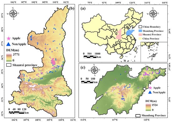
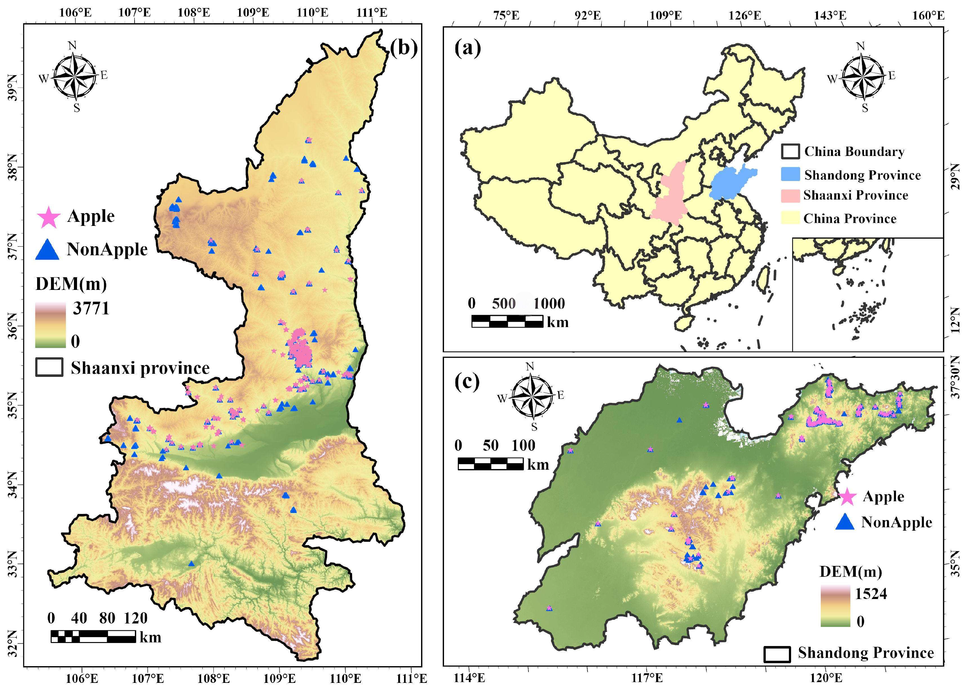
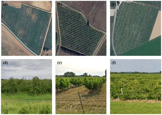
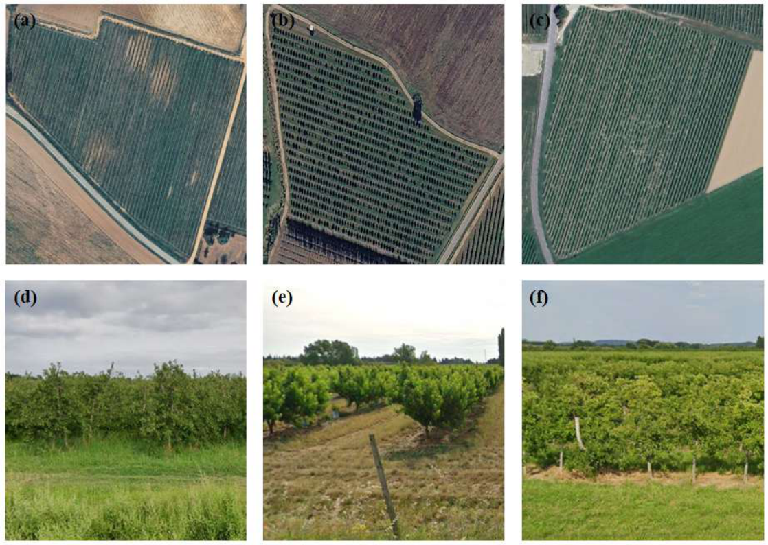
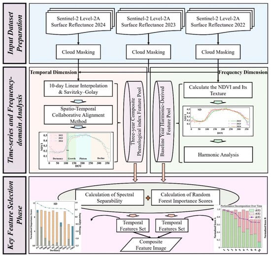
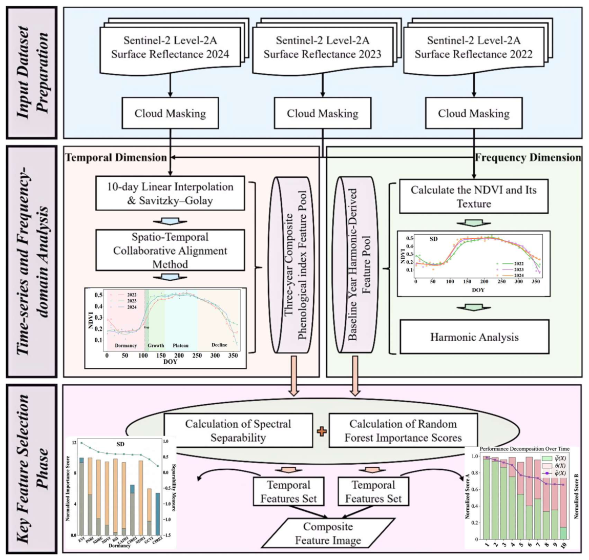
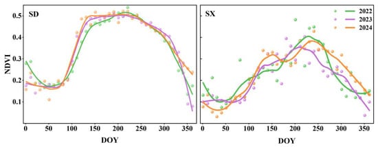
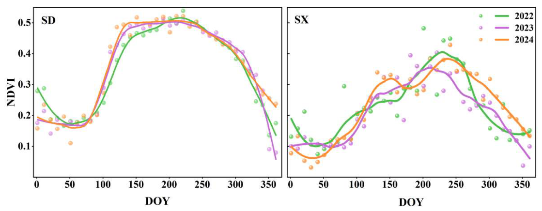
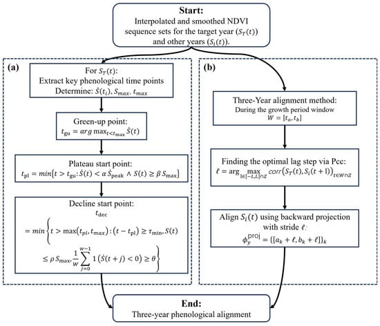
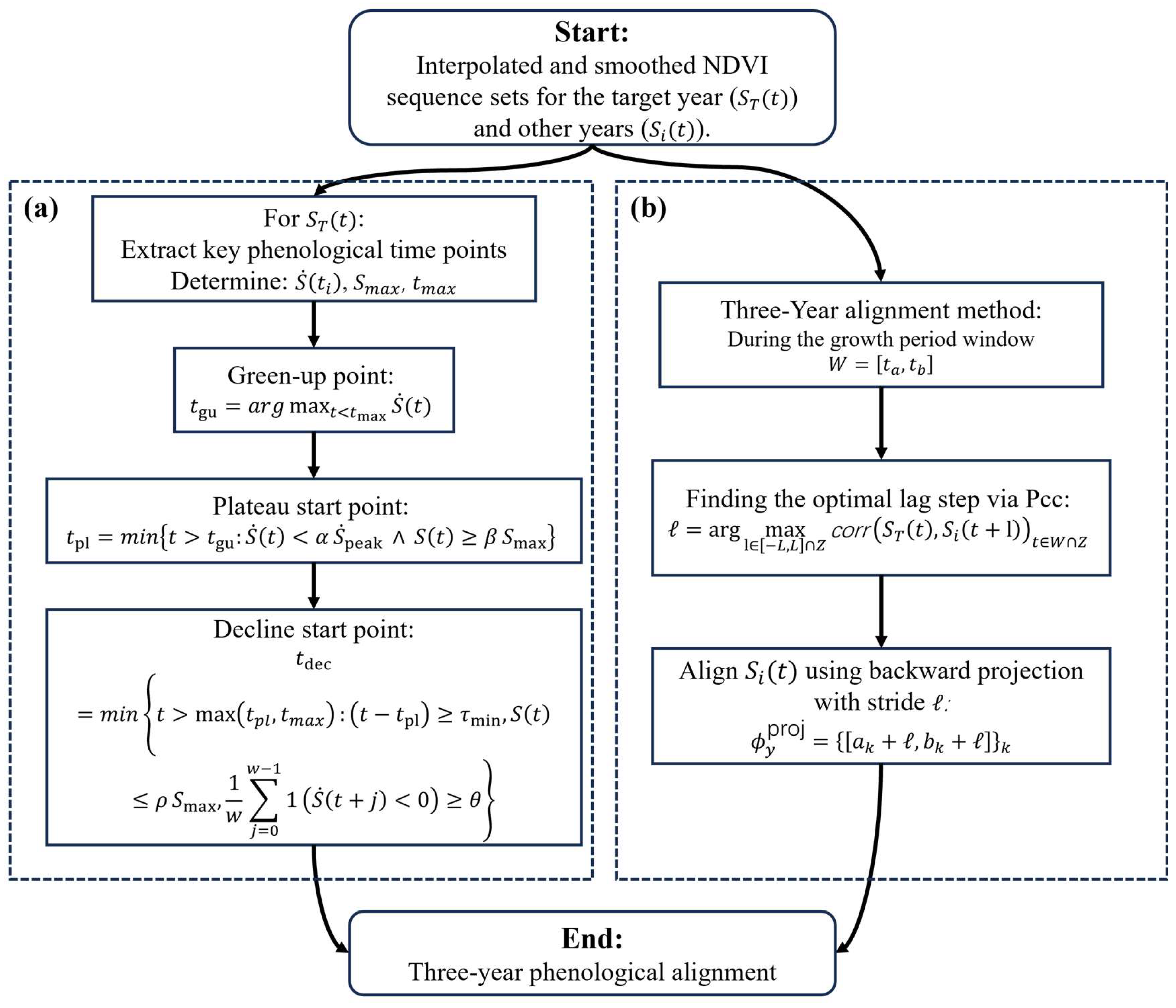
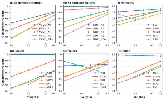
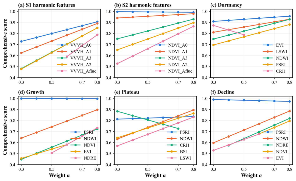
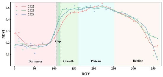
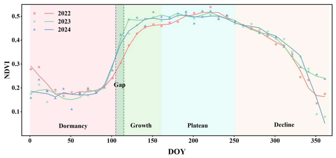
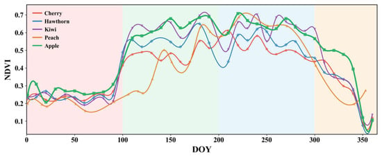
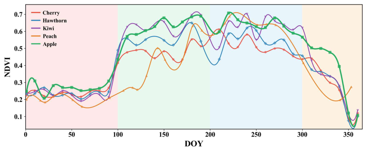
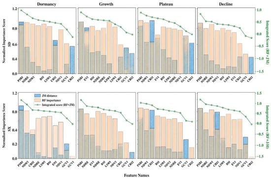
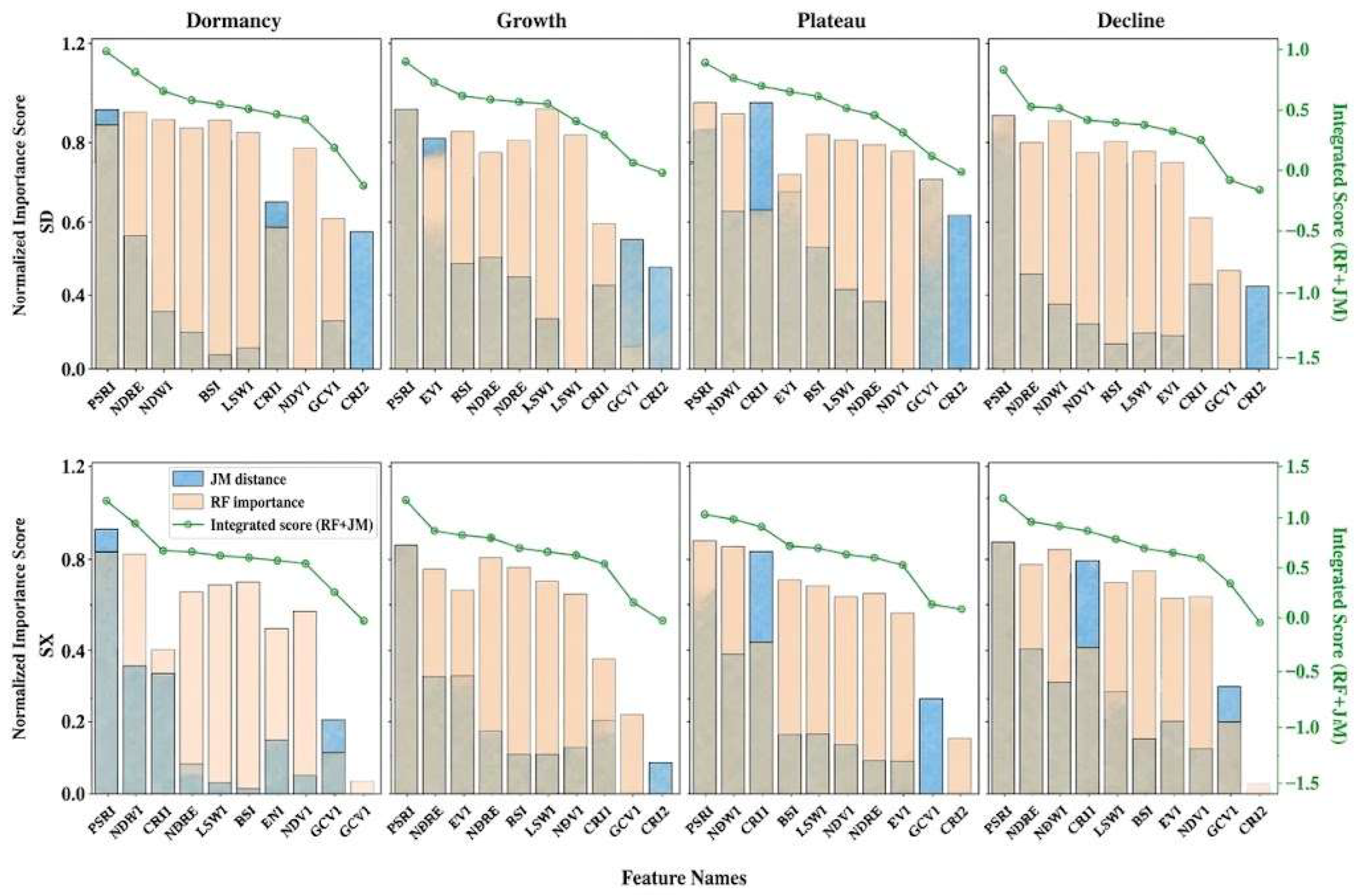
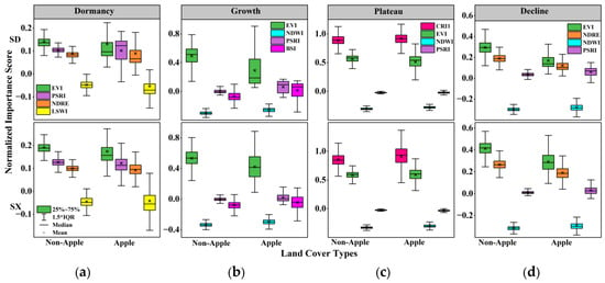
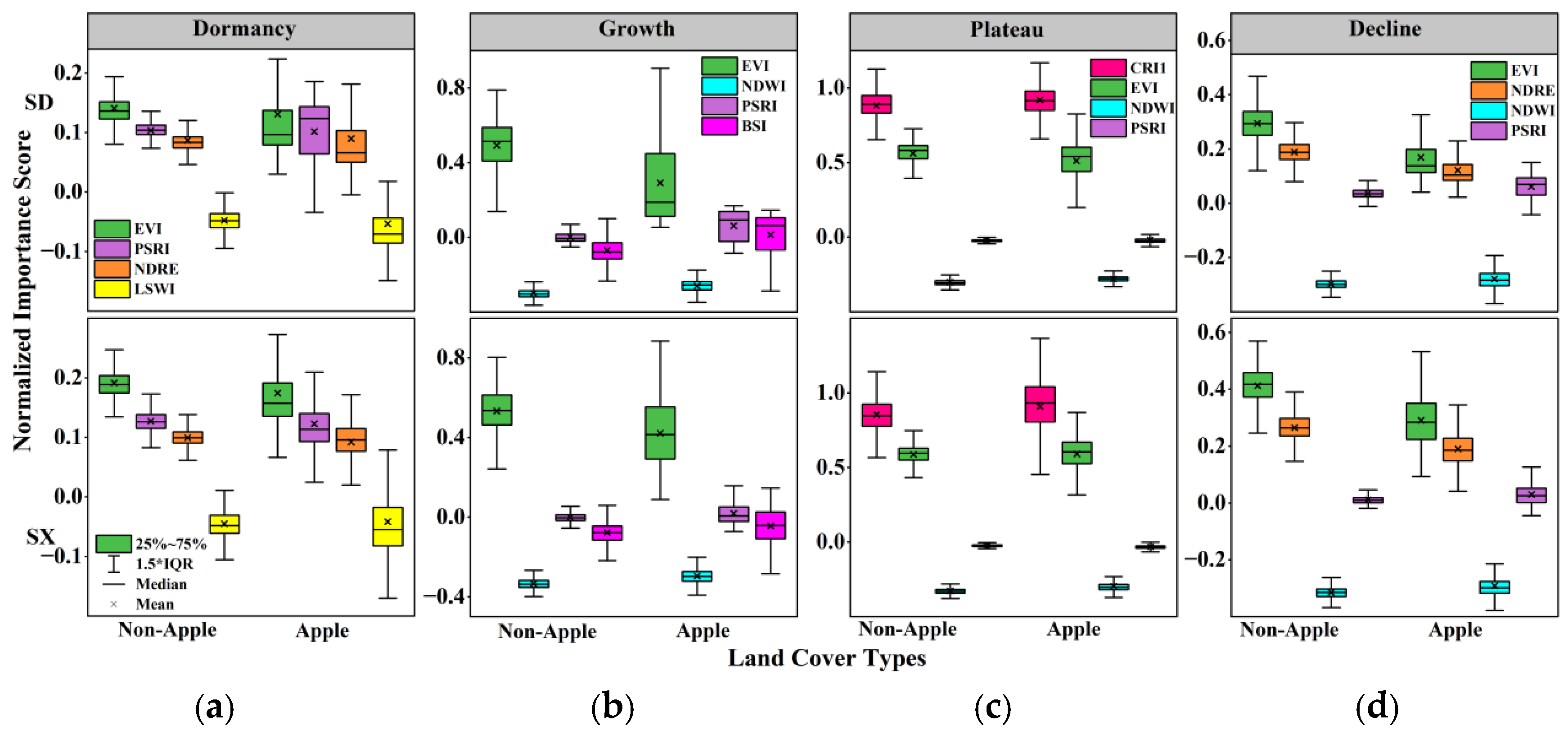
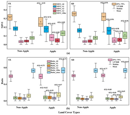
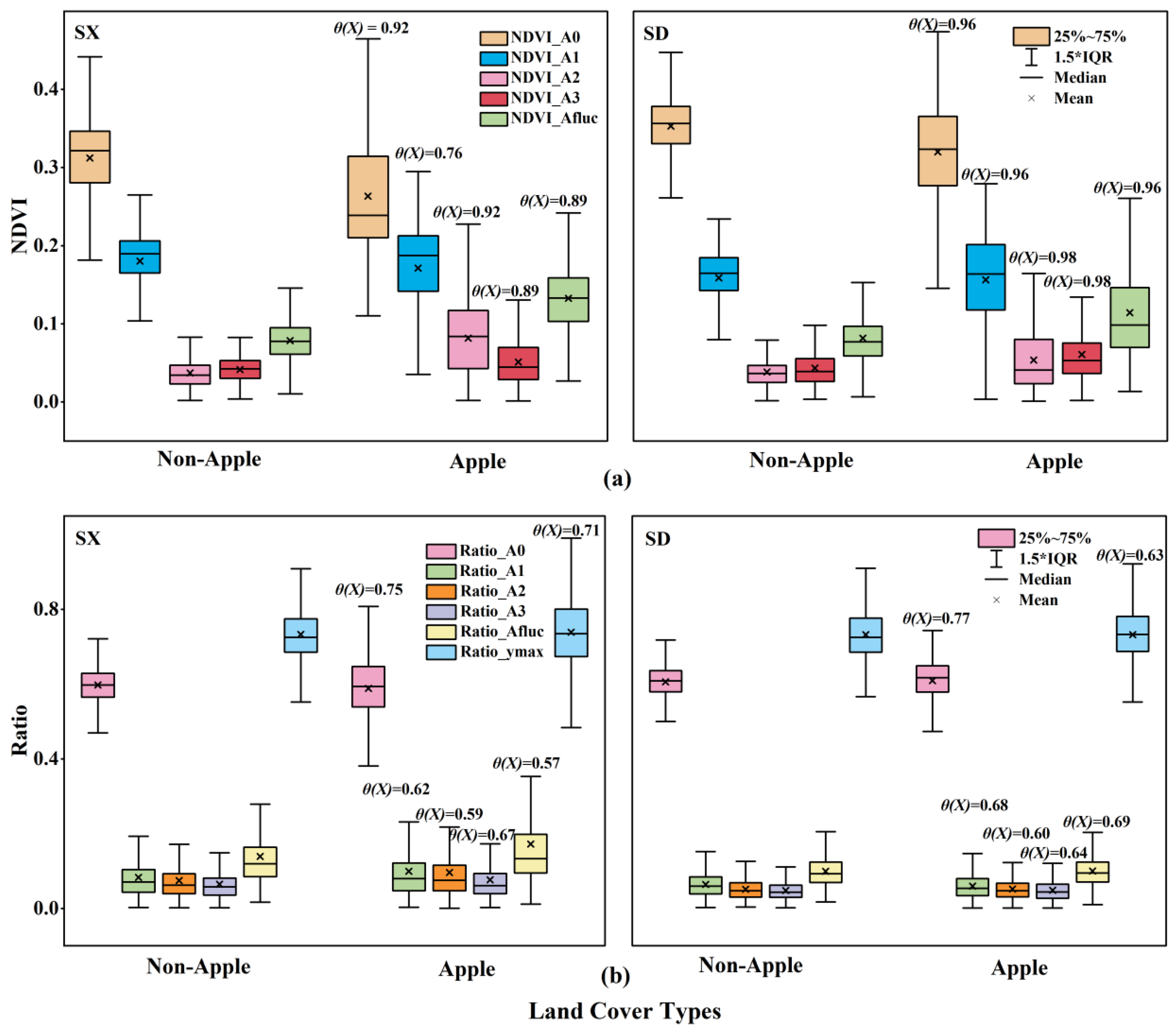
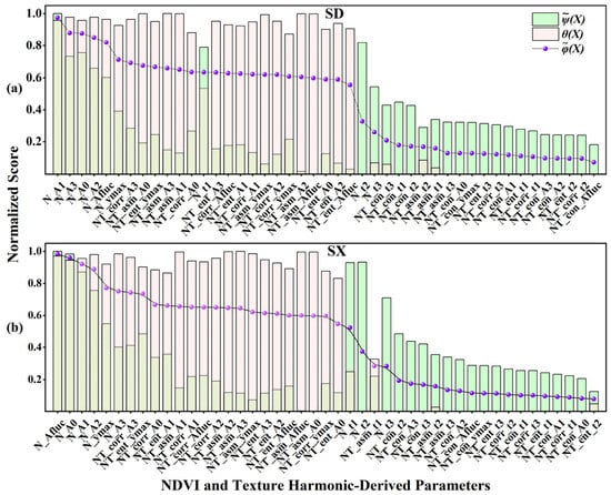
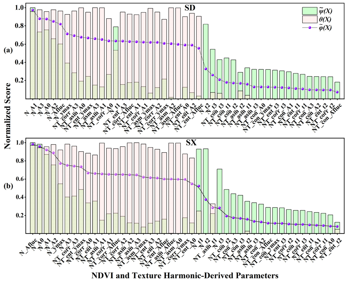
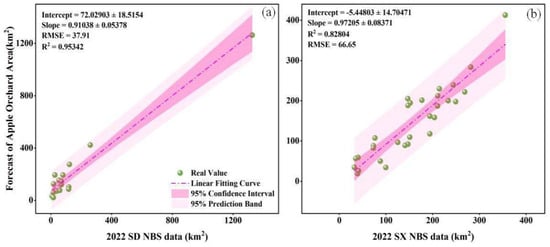
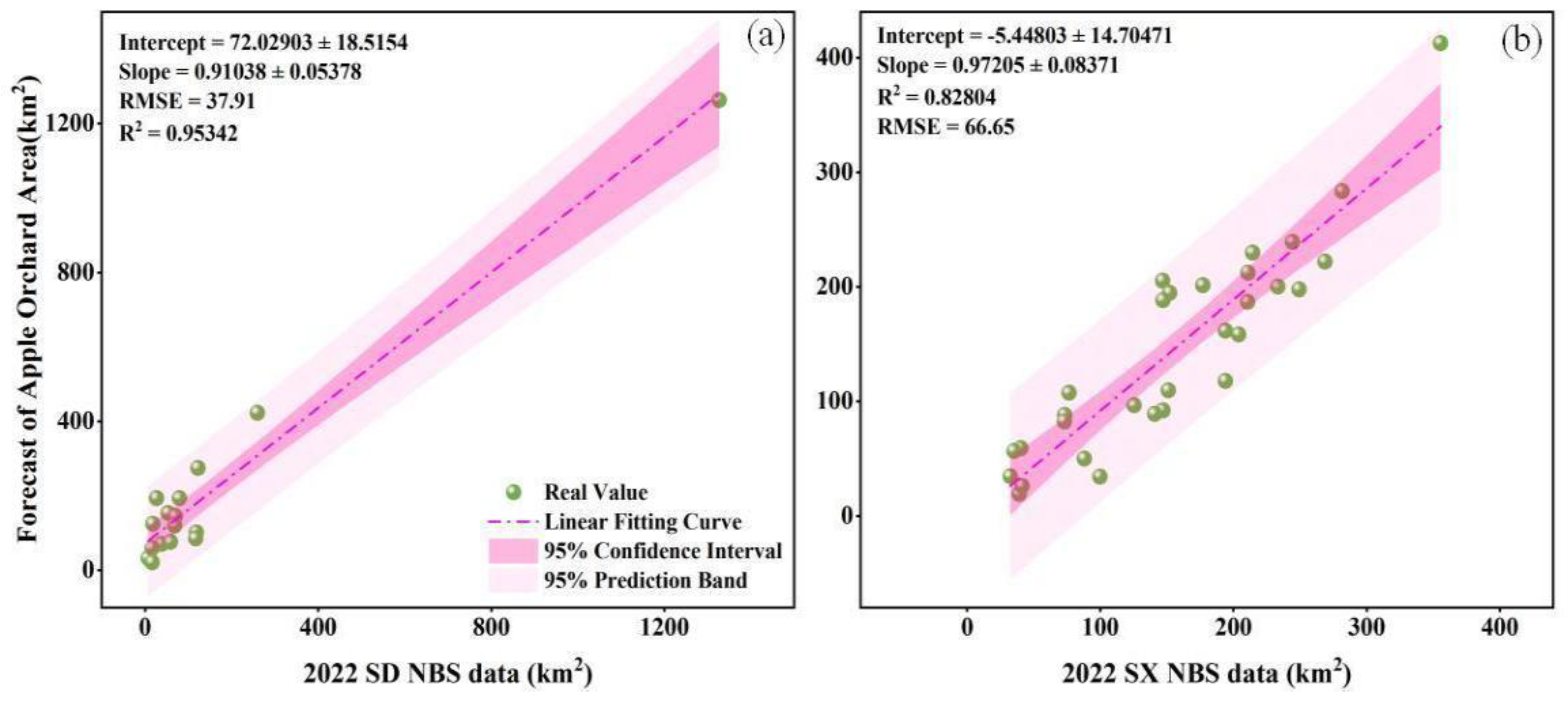
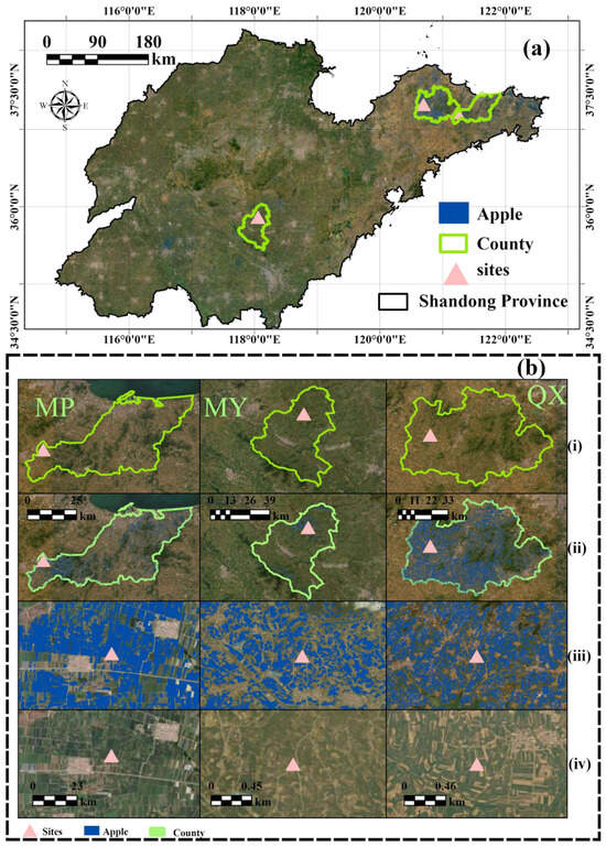
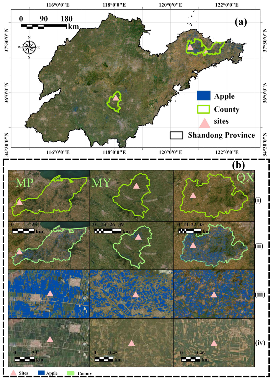
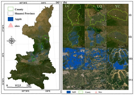
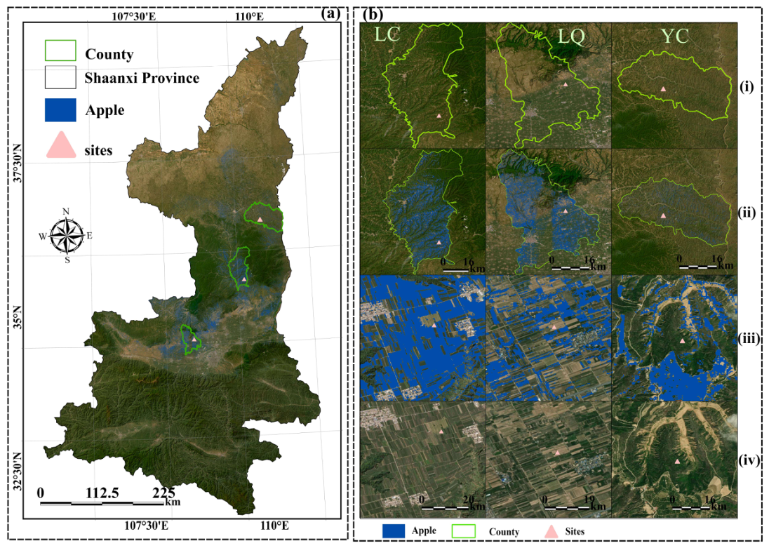

Disclaimer/Publisher’s Note: The statements, opinions and data contained in all publications are solely those of the individual author(s) and contributor(s) and not of MDPI and/or the editor(s). MDPI and/or the editor(s) disclaim responsibility for any injury to people or property resulting from any ideas, methods, instructions or products referred to in the content. |
© 2026 by the authors. Licensee MDPI, Basel, Switzerland. This article is an open access article distributed under the terms and conditions of the Creative Commons Attribution (CC BY) license.