


Highlights
What are the main findings?
- GUF-Net derives evidential pixel-level uncertainty directly supervised by a redesigned evidential loss and routes it through a dynamic gated fusion module, departing from prior auxiliary uncertainty signals that lack explicit task-aligned supervision and are validated only on clean benchmarks.
- Under the strongest Gaussian, salt-and-pepper, and speckle noise conditions, GUF-Net’s F1 decreases by only 0.86, 3.95, and 1.29 percentage points, respectively, showing the smallest degradation among the compared models.
What are the implications of the main findings?
- Uncertainty-guided gating can help suppress unreliable responses and reduce noise-induced false changes under degraded input conditions.
- When combined with multi-scale representations and supporting global contextual information, uncertainty-aware feature fusion can preserve change details while improving robustness in noisy remote sensing change detection.
Abstract
Building change detection (BCD) in high-resolution remote sensing imagery has achieved considerable accuracy with deep learning, yet most existing models still suffer from performance degradation under noise interference, partly due to inadequate uncertainty handling. To address this, we propose GUF-Net, a gated uncertainty-aware fusion network that integrates three key components: (1) a pixel-wise uncertainty modeling module that generates a pixel-level uncertainty map alongside the change probability map; (2) an adaptive gated fusion mechanism that dynamically weights multi-scale features and uncertainty information; and (3) a redesigned loss function that can directly supervise the uncertainty estimation, ensuring that it reflects prediction reliability rather than serving as an unsupervised auxiliary output. Experiments on three public benchmarks (WHU-CD, CDD, and LEVIR-CD) show that GUF-Net achieves competitive F1 scores of 93.88%, 96.55%, and 90.43%, respectively, ranking top three on CDD and WHU-CD, while its advantage is less pronounced on LEVIR-CD. Under the strongest Gaussian, salt-and-pepper, and speckle noise conditions on the WHU-CD test set, the F1 score of GUF-Net decreases by only 0.86, 3.95, and 1.29 percentage points, respectively, exhibiting the smallest degradation among the compared models. Unlike existing uncertainty-aware baselines evaluated solely on clean data, GUF-Net jointly supervises evidential pixel uncertainty and routes it through adaptive gating, enabling stable fusion under degraded imaging conditions. Ablation studies confirm that the gated fusion, uncertainty injection, and global context aggregation each contribute to the overall performance. These results suggest that explicit uncertainty modeling and adaptive fusion can improve the reliability of BCD under noisy conditions, although there remains room for further improvement in clean-set accuracy and model efficiency.
1. Introduction
Remote sensing image change detection identifies the temporal changes in ground objects by comparing multi-temporal images of the same geographic area, which is one of the core tasks in remote sensing information analysis [1]. Building change detection (BCD), as an important branch of land-cover change detection, aims to accurately identify building construction, demolition, and reconstruction activities. It provides essential data support for urban planning [2], disaster emergency response [3], and land resource management [4]. With the development of deep-learning-based BCD models, building textures, contours, and fine-grained structures can be effectively identified. Currently, uncertainties arising from complex scenarios have become a major bottleneck restricting detection accuracy.
Uncertainties in BCD can be categorized into two groups. One group arises from data acquisition and annotation. Data acquisition factors, such as differences in sensor viewing angles, variations in illumination conditions, and atmospheric interference, can cause spectral differences in the same object across multitemporal images, which easily introduce pseudo-change information [5]. In addition, uncertainty arises from data annotation. For example, the LEVIR-CD dataset contains manual annotation errors, and the changed pixels account for only 4.63%, where the severe class imbalance further intensifies data uncertainty in real-world applications [6,7]. The other group arises from data processing. Biases in feature extraction, prediction fluctuations, and the risk of overfitting in deep learning networks may lead to inaccurate predictions in ambiguous regions of complex scenes [8]. Traditional change detection methods struggle to handle these challenges [9]. While pixel-based approaches focus solely on the spectral differences in individual pixels, making them highly sensitive to noise [10], object-based approaches rely on extracted features and the quality of multi-scale segmentation, resulting in limited generalization capability [11,12].
The rise of deep learning techniques has provided new solutions for BCD. Gong et al. [13] were among the first to apply convolutional neural networks (CNNs) to change detection. Owing to their strong local feature extraction capability, CNNs subsequently became a mainstream approach. Subsequent studies have continuously improved their performance through various strategies, e.g., dense connections [14] and self-attention mechanisms [15]. However, the local receptive fields of CNNs limit their ability to capture global contextual information. In scenes containing buildings with substantial scale variations and complex spatial distributions, CNN-based models are sensitive to noise and other uncertain perturbations, which may lead to missed detections and false alarms [16]. More recently, Transformer models have been introduced to effectively capture long-range dependencies through the self-attention mechanism. The Bi-temporal Image Transformer (BIT) proposed by Chen et al. [17] has advantages in global modeling on multiple datasets. However, the initial Transformer architecture suffers from deficiencies in preserving local details and resisting noise interference, along with high computational cost.
Hybrid models have emerged to integrate the advantages of the above-mentioned CNNs and Transformers. Previous hybrid models have achieved promising results. For example, USSFC-Net [18] achieved efficient feature extraction via multi-scale decoupled convolution and the spatial–spectral Transformer-based feature fusion strategy. ChangeFormer [19] adopted a hierarchical Transformer structure to balance global and local information extracted by CNN. However, existing hybrid models still have three limitations in handling uncertainty. (1) Current models lack specific quantification of uncertainty, thereby failing to accurately characterize the certainty of pixel-level predictions [7]. (2) Current feature fusion and uncertainty processing methods are static, making it difficult to adapt to the data distribution dynamics under complex scenarios [20]. (3) Global semantic information is not fully exploited for uncertainty weighting. Transformer-based global context (e.g., GCFormer [21]) is often used only for feature enhancement rather than pixel-wise uncertainty weight generation, leading to notable F1/IoU degradation under noise.
Recently, uncertainty-aware BCD methods (e.g., UA-BCD [7], SA-CDNet [22], UBA [23], UACD [24]) have improved detection accuracy on standard benchmarks. However, none of them systematically evaluates model behavior under noise-corrupted imaging conditions, leaving their robustness boundaries largely unknown. We revisit these methods in more detail in Section 2.2.
To address the above issues, this paper proposes a gated uncertainty-aware fusion network (GUF-Net) to quantify and employ pixel-level uncertainty in feature fusion. Distinct from existing uncertainty-aware baselines, GUF-Net couples explicitly supervised evidential uncertainty with adaptive uncertainty-conditioned gating, allowing the network to downweight unreliable activations while preserving discriminative change details. The proposed framework contributes in two aspects:
- (1)
- A pixel-level uncertainty quantification module and a gated fusion mechanism were designed. Explicit uncertainty modeling was implemented via dual-channel output of change probability and uncertainty value. A dynamic gating mechanism performed single-stage fusion of deep decoder features and averaged uncertainty information. In addition, the loss function was redesigned to directly supervise the uncertainty estimation, ensuring that it genuinely reflects prediction reliability rather than serving as an unsupervised auxiliary output.
- (2)
- GUF-Net’s strong noise robustness was demonstrated in diverse simulated noisy environments. Through comparative experiments with three types of noise at three levels added to the images, GUF-Net exhibited significantly lower performance degradation than other methods in the strongest noisy conditions, effectively handling uncertainty challenges caused by noise.
2. Related Work
This section provides an overview of uncertainty in BCD, recent advances in uncertainty modeling, and techniques that combine feature fusion strategies with uncertainty awareness.
2.1. Sources and Challenges of Uncertainty in BCD
According to uncertainty theory, these challenges can be systematically categorized into aleatoric uncertainty, which arises from data acquisition and annotation, and epistemic uncertainty, which arises from data processing. These two types of uncertainty are intertwined, constituting the core challenge of current BCD research.
2.1.1. Uncertainty from Data Acquisition and Annotation
Uncertainty from data acquisition and annotation mainly arises from disturbances and ambiguities introduced during the remote sensing imaging process and subsequent data preparation steps. Sensor noise (e.g., thermal noise and photon noise), which is inherent in imaging systems, may cause observed pixel values to deviate from the underlying surface radiance or reflectance. In high-resolution images (e.g., 0.5 m/pixel in the LEVIR-CD dataset), small radiometric disturbances may be mistaken for changes along building edges or in roof textures [6]. In addition, environmental and acquisition factors, such as illumination differences, atmospheric scattering and absorption, cloud cover, and seasonal vegetation changes, can lead to significant spectral differences in the same object between images acquired at different times. These factors may introduce pseudo-changes even when no actual semantic change has occurred [6,7]. In unaligned change detection scenarios (e.g., differences in sensor viewing geometry or terrain-induced displacement), pixel-level comparison and feature correspondence become considerably more difficult. Previous studies have shown that image misalignment can introduce spurious changes and degrade change detection performance, highlighting the significant impact of data misalignment on detection results [25].
In addition, the subjectivity of manual annotation and the imbalance of class distribution affect different stages of the change detection process. Differences in semantic interpretation during annotation (e.g., whether changes involving roads or bridges should be classified as building changes) may lead to erroneous annotations. Li et al. [7] noted that background objects resembling buildings, such as roads and bridges, may be incorrectly annotated as building changes, thereby introducing data-level aleatoric uncertainty. Meanwhile, LEVIR-CD exhibits severe class imbalance, with changed pixels accounting for only approximately 4.63% of all pixels, as shown in Table 1. This imbalance may bias the model toward the unchanged class and weaken its ability to learn features from the minority changed class, thereby increasing the risk of missed detections. Furthermore, limitations in sensor resolution may cause small buildings to occupy only a few pixels, making their boundaries and semantic categories difficult to determine. The temporal intervals between paired images in the LEVIR-CD dataset range from 5 to 14 years [6]. Such long intervals may increase accumulated variations in seasons, surface materials, and object appearance, making actual building changes more difficult to distinguish from nuisance changes and further amplifying uncertainty.
Table 1.
Summary information for the LEVIR-CD dataset [6].
2.1.2. Uncertainty from Data Processing
Uncertainty from data processing mainly comes from the inherent limitations of the model structure. Specifically, model-parameter stability, overfitting, and training data insufficiency may cause inconsistent data processing results, leading to uncertainty in prediction. As two mainstream architectures for BCD, both CNNs and Transformers have limitations in data processing. Because their local receptive fields limit their ability to capture global contextual information of buildings, CNNs are prone to missing small objects (e.g., single-story buildings) or producing blurred boundaries when handling scenes with large-scale differences [26]. On the other hand, Transformer-based methods may overlook fine-grained spatial information, resulting in poor boundary integrity and the loss of small changed objects [27]. Although hybrid models have attempted to integrate the strengths of CNNs and Transformers, the effective interaction and fusion of multi-scale bi-temporal features remain challenging. For example, simple or unidirectional connections between CNN and Transformer features may lead to information loss during inter-scale communication, thereby weakening the detection of small changed objects and boundary details [28].
Training limitations further amplify uncertainty. Limited annotated samples cannot cover all building change patterns and background complexity in the real world, causing the model to overfit the training set and reducing its generalization ability to new scenes or noise disturbances. This is particularly evident under conditions of small sample sizes [8]. Robustness experiments further demonstrate that change detection models can be sensitive to input degradation. For example, experiments on the LEVIR-CD+ dataset showed that Gaussian noise caused F1 score drops ranging from 15.07% to 40.83% for several representative change detection models [29]. In addition, most existing models lack effective confidence estimation mechanisms and cannot distinguish reliable predictions from random guesses.
To summarize, noise disturbance and annotation bias, structural limitations, and training bias interact and cause uncertainty and errors in complex BCD scenarios. These uncertainties directly limit the effectiveness of models in real applications. Therefore, how to effectively model and fuse multi-source uncertainties and continuously optimize feature fusion strategies has become a key research direction for improving the robustness and reliability of BCD models.
2.2. Deep Learning in Uncertainty Modeling
To address the challenges brought by uncertainty in BCD, researchers have developed a series of methods to quantify, model, or reduce uncertainty. Among these methods, deep learning methods have become the main approach.
Specifically, Bayesian Neural Networks (BNNs) place probability distributions over network weights and use variational inference to approximate the posterior distribution, thereby enabling predictive uncertainty to be quantified [30]. In addition, ensemble learning and adversarial learning have been explored to improve prediction reliability and model robustness in remote sensing change detection. For example, Yang et al. [31] combined the outputs of multiple change detection models to improve pseudo-label quality under limited annotations. Chen et al. [32] employed generative adversarial training to synthesize diverse bi-temporal building-change samples, thereby alleviating training-data scarcity and improving model generalization.
Loss function design also plays a key role in uncertainty modeling [33]. In change detection, the dynamic adaptive focal loss dynamically adjusts the weights of changed and unchanged samples according to their distribution in each training batch and adapts the weights of hard samples based on changes in label-prediction probabilities during training, thereby enhancing the learning of hard-to-classify changed regions. On the LEVIR-CD dataset, it improved the F1 score by 3.89% in small-sample settings [20]. In addition, the enhanced focal contrastive loss introduces contrastive margins into the metric learning framework, which alleviates class imbalance and improves feature discriminability. Spatial attention mechanisms generate spatial weight maps to enhance the features of building regions and suppress background noise, yet they still exhibit insufficient robustness in high-noise scenarios [34].
Recent studies have begun to explicitly model and exploit uncertainty in BCD. Li et al. [7] proposed the UA-BCD framework, which systematically distinguishes between aleatoric uncertainty arising from data noise and epistemic uncertainty stemming from model limitations. The framework employs a conditional variational autoencoder to estimate aleatoric uncertainty and an entropy-supervised cognitive uncertainty estimator to guide the model in generating change maps with low uncertainty, achieving superior performance across five public building change detection datasets. Subsequently, Gan et al. [22] introduced SA-CDNet, which integrates frozen FastSAM visual foundation models to extract semantic priors and designs a dual-stream feature decoder to mine both semantic-aware and difference-aware features. The method achieved state-of-the-art results on multiple benchmark datasets, including LEVIR-CD, S2Looking, and WHU-CD. Furthermore, Di et al. [23] proposed the Uncertainty-Guided Bayesian Adaptation (UBA) framework, a plug-and-play module that semantically associates aleatoric and epistemic uncertainties with building edges and minority changed classes, respectively, and dynamically reweights the loss function using uncertainty maps. This approach yielded significant improvements in mIoU and F1 scores across several mainstream BCD methods. More recently, a UACD [24] framework was proposed as a plug-and-play solution, embedding Monte Carlo Dropout at multiple network positions to estimate pixel-level uncertainty and adding an uncertainty-guided regularization term for end-to-end fine-tuning. This approach demonstrates consistent gains across CNN-, Transformer-, and foundation-model-based architectures on four benchmark datasets.
Despite these advances, the robustness of these methods under noisy inputs has not been systematically evaluated. UA-BCD was tested only on standard clean test sets, with no noise injection experiments. SA-CDNet, although motivated by the challenge of noise and illumination variations, also reports results on clean benchmarks only. The UBA framework explicitly identifies image noise as a core challenge but provides no quantitative assessment under controlled noise. UACD, while attributing aleatoric uncertainty to data acquisition noise, similarly lacks noise robustness experiments. Consequently, the extent to which uncertainty-aware models can maintain reliability when inputs are corrupted by noise remains largely unknown. This gap motivates the noise-robust design and evaluation conducted in this work.
2.3. Integrating Uncertainty Awareness in Feature Fusion
Note that this work extends our previous study [35], which shares two co-authors with this work. However, the proposed architecture substantially differs from [35]: the THFA module is a lightweight global context extractor, while the GUF module, the uncertainty estimation branch, and the uncertainty-conditioned gating mechanism are newly introduced and constitute the main contributions of this paper.
Feature fusion integrated with uncertainty awareness offers significant potential in improving BCD performance. Related studies mainly focus on feature-level fusion and decision-level fusion.
Feature-level fusion aims to improve change detection accuracy by effectively integrating multi-scale features and uncertainty information. SLDDNet [36] cascaded CNN with Transformer, using self-attention to suppress noisy activations and enhance feature discriminability. CTD-Former [37] introduced an uncertainty-aware attention module on multi-scale difference maps to dynamically adjust the feature weights of unreliable spatiotemporal positions. These methods were computationally efficient, but they did not explicitly model the uncertainty distribution, which could limit their ability to capture complex changes. On the other hand, decision-level fusion aggregated the outputs of multiple models to achieve higher confidence and accuracy. Deep Ensemble and Snapshot Ensemble methods improve calibrated confidence by combining the predictions of multiple models. For deep ensembles, the calibration/uncertainty error typically follows a power-law-like decay with ensemble size and exhibits diminishing returns as the number of members increases [38]. Snapshot ensembles similarly yield further gains with more snapshots, but the marginal improvement tends to saturate once diverse loss-landscape modes are sufficiently covered. However, computational cost increases dramatically during inference, making it difficult for this method to meet real-time application requirements, especially in large-scale real-time change detection scenarios.
One of the noteworthy feature fusion frameworks in uncertainty processing is the gating mechanism, which can utilize learnable weights to dynamically adjust feature flow. In DFANet, GatedConv is combined with a spatial-channel attention module to recalibrate features, highlight change-related information, and suppress irrelevant background responses. On the LEVIR-CD dataset, incorporating the spatial-channel attention and GatedConv modules improved the F1 score by 2.21 percentage points over the baseline [39]. Similarly, MSGFNet employs a multi-scale gated fusion module to adaptively fuse multi-scale bi-temporal features. This module helps preserve boundary details and detect completely changed targets. MSGFNet achieved F1 scores of 90.86%, 92.46%, and 80.39% on the LEVIR-CD, WHU-CD, and SYSU-CD datasets, respectively [40].
Although gating-based methods have been proven effective for handling uncertainty, current approaches still suffer from two shortcomings: (1) static weight adjustment that lacks dynamic regulation over the feature space and fails to respond to uncertainty, and (2) insufficient evaluation under diverse noise-corrupted inputs, leaving it unclear whether their fusion strategies can reliably suppress noise-induced false responses in practical change-detection scenarios.
To this end, this paper proposes GUF-Net, a dynamic gated uncertainty fusion framework that adaptively fuses uncertainty information with multi-scale features. Rather than performing fixed channel-wise reweighting, the module dynamically modulates deep decoder features and spatially aligned uncertainty cues at each pixel. Beyond clean-set evaluation, GUF-Net is systematically benchmarked across multiple noise types and severity levels, offering a more rigorous robustness assessment for uncertainty-guided BCD.
3. Methods
3.1. Overall Framework of GUF-Net
The overall framework of the proposed GUF-Net model is based on the classic U-Net structure, including the encoder and the decoder. To better extract features, estimate uncertainty, and fuse features and uncertainty, we designed the Transformer-based Hierarchical Feature Aggregator (THFA) module and the Gated Uncertainty Fusion (GUF) module. The loss function was also redesigned to supervise uncertainty estimation.
As shown in Figure 1, GUF-Net employs two structurally identical encoder branches without weight sharing to process the T1 and T2 images independently. No concatenation or fusion is performed between the two temporal images before they enter their respective encoders. After feature extraction at each encoding stage, the element-wise absolute difference between the corresponding features of the two branches is computed. The difference features generated from Stage 0 to Stage 3 are used as skip connections and concatenated along the channel dimension with the upsampled features at the corresponding decoding stages. The deep difference feature generated at Stage 4 is fed into the THFA module to model global change relationships and provide global semantic support for subsequent feature fusion. By combining explicit uncertainty modeling with a modified gating mechanism, GUF-Net performs single-stage uncertainty-guided fusion between the averaged Stage 4 uncertainty map and deep decoder features, thereby enhancing the model’s adaptability to noise and complex backgrounds.
Figure 1.
The overall framework of the GUF-Net model.
The decoder adopts a symmetric U-Net architecture and restores the resolution of feature maps through transposed convolution with layer-wise upsampling. In Decoder 1, the gating mechanism dynamically fuses the uncertainty maps output from Stage 4 in the encoder with the upsampled decoder features. After enhancement by channel and spatial attention mechanisms, fine-grained feature representations are generated. The final output layer employs an uncertainty-aware module to produce a dual-channel result of change probability and uncertainty value.
3.2. Feature Extraction
Feature extraction in GUF-Net is realized based on a modified USSFC [18] encoder and a THFA module. The encoder adopts a Siamese architecture without weight sharing and consists of five stages (Stage 0–Stage 4) that progressively reduce the spatial resolution of input images while increasing the depth of feature maps. As shown in Figure 1 and Table 2, a multi-stage differentiated feature processing strategy is employed to effectively model multi-scale information and uncertainty. Specifically, Stage 0 applies standard convolution to the input raw image for initial shallow feature extraction; Stages 1–3 use the proposed Depth-wise Separable Dilated Convolution with Double Attention Mechanism (DSDConv_DA), which extracts multi-scale dilated features and enhances sensitivity to key features through the attention mechanism; Stage 4 further introduces an uncertainty output module on top of DSDConv_DA to quantify the model’s prediction uncertainty in different regions and generate dual outputs consisting of an auxiliary change probability map and a pixel-level uncertainty map, while retaining the deep feature map for subsequent difference modeling. The THFA module is positioned between the encoder and decoder, capturing long-range dependencies in deep features through self-attention mechanisms and thereby providing global semantic support for the gated fusion.
Table 2.
Configuration of a single temporal encoder branch and inter-temporal operations in the dual-branch GUF-Net encoder.
As shown in Figure 2b, the input feature map first passes through the DSDConv_DA to capture both local details and wide contextual information. Then, a 2D dropout is applied, randomly zeroing feature elements at a preset probability, allowing the model to learn diverse feature representations during training and reducing overfitting. In addition, batch normalization and ReLU activation are employed to enhance numerical stability and non-linear representation capacity. This process is repeated across Stage 1 to Stage 3 to optimize feature representation.
Figure 2.
Feature extraction process in GUF-Net: (a) Uncertainty output module; (b) Feature extraction process based on DSDConv_DA.
The DSDConv_DA was designed based on the MSDConv module proposed by the USSFC model and modified with a spatial-channel dual attention module. As shown in Figure 3, this module consists of two parallel feature extraction branches: the raw feature extraction branch (orange arrows) and the depth-wise separable dilated convolution branch combined with spatial-channel attention, i.e., the DSDConv_DA branch (blue arrows). In the raw feature extraction branch, standard convolution operations are used to extract basic features, combined with batch normalization and ReLU activation to ensure effective capture of the main features of the input tensor.
Figure 3.
The feature extraction module based on DSDConv_DA.
The DSDConv part of the DSDConv_DA module integrates multi-scale dilated convolutions, depth-wise separable convolutions, and standard convolutions, enabling the model to retain rich multi-scale information while remaining lightweight to improve computational efficiency. As shown in Figure 4, this module first implements multi-scale dilated convolutions using three different dilation rates. Smaller dilation rates are used to focus on extracting local features, while larger dilation rates capture more distant contextual information. Then, the depth-wise separable convolution module decomposes standard convolution into depth-wise convolution and pointwise convolution, enhancing both flexibility and efficiency in feature extraction. The depth-wise convolution applies convolution independently to each input channel, whereas the pointwise convolution uses 1 × 1 kernels to integrate information across channels. The output of the depth-wise convolution can be expressed as:
where Xk denotes the kth input channel, and denotes the depth-wise convolution kernel corresponding to the kth input channel. This operation is performed independently for each input channel and does not involve summation across different input channels. Subsequently, the pointwise convolution uses 1 × 1 kernels to integrate information across channels, and its output can be expressed as:
where Wj,k is the weight matrix of the pointwise convolution. Through these two steps, the output of the jth channel depth-wise separable convolution can be expressed as Equation (3):
Figure 4.
Schematic diagram of the DSDConv_DA feature extraction module.
To further enhance the representational capability of the feature maps, this study also introduces a spatial-channel dual attention mechanism, including spatial attention and channel attention, which optimize the feature maps along spatial and channel dimensions, respectively. The spatial attention mechanism learns the importance of each spatial location, assigning a weight Aspatial to each position in the feature map, allowing the model to focus more on key regions. Its output can be expressed as Equation (4):
Aspatial = σ(Convspatial(X))
In Equation (4), Convspatial is a 1 × 1 convolution layer used to generate the spatial attention map from the input feature map, and σ denotes the sigmoid activation function. The channel attention is computed by the following two equations:
Y = Conv1(AvgPool(X))
Achannel = σ(Conv2(ReLU(Y)))
As shown in Equations (5) and (6), in the channel attention mechanism, Conv1 and Conv2 correspond to the first and second convolution layers of the channel attention module. Global average pooling is used to generate a global feature representation Y for each channel, effectively aggregating information across spatial dimensions. Then, Y passes through the first convolution followed by a ReLU activation, and subsequently through the second convolution, producing the channel attention map Achannel, which reflects the importance of each channel’s features. Finally, in the final stage of feature enhancement, the input feature map is subjected to element-wise multiplication weighting by combining the channel attention map and spatial attention map, generating the enhanced feature representation denoted as XDA, whose mathematical expression is given as follows:
XDA = Xinput⨀Achannel⨀Aspatial
In Equation (7), ⨀ denotes element-wise multiplication. The output enhanced by the channel and spatial attention mechanisms, after this element-wise multiplication, effectively strengthens the model’s sensitivity to important features, making the representation of key regions in the feature map more prominent.
In addition to the encoder, we employ the THFA module as a supporting global-context extractor to integrate local change responses with broader semantic relationships across the image. By leveraging Transformer self-attention, THFA captures long-range dependencies among remote sensing image features [41] and provides contextual information for the subsequent uncertainty-guided fusion process.
The THFA module is positioned between the encoder and the decoder, taking the deep features from Stage 4 as input. The selection of these deep features considers two factors: (1) Deep features carry richer semantic information and global context, which helps capture subtle changes in images and improves accuracy. (2) The model complexity and parameter size can be effectively controlled to avoid computational burden and overfitting risk that may arise from incorporating shallow features.
As shown in Figure 5, the THFA module takes the multi-scale deep features X ∈ ℝB×C×H×W generated by the encoder’s last convolutional layer as input, where B is the batch size, C is the number of channels, and H and W denote the height and width of the feature map, respectively. After entering the THFA module, the feature map X is reshaped into a sequence format through a linear projection, denoted as Xseq ∈ ℝB×(HW)×C. Subsequently, the reshaped features are used to generate the query, key, and value triplets for the self-attention mechanism. The specific attention computation is given by the following equation:
Figure 5.
The schematic diagram of the THFA module framework.
In Equation (8), dk denotes the feature dimension of the query and key in each attention head. Since eight attention heads are employed in this study, dk is set to one-eighth of the total channel dimension. The scaling factor controls the magnitude of the query–key dot products and prevents the Softmax function from becoming overly saturated, thereby improving the numerical stability of the attention computation. Through this self-attention mechanism, the model can dynamically compute the relationships between features and adjust attention weights, thereby significantly enhancing the focus on key features. This aims to effectively suppress interference during feature fusion, ensuring that the model can more accurately identify and distinguish building changes in complex scenarios, thus improving overall adaptability and stability.
Furthermore, to achieve hierarchical feature aggregation and feature propagation, the THFA module adopts a hierarchical Transformer architecture consisting of L = 6 consecutively stacked Transformer blocks. Each Transformer block comprises an eight-head self-attention mechanism and a feedforward neural network (FNN), as shown in Figure 5, together with residual connections and layer normalization to enhance information propagation and feature extraction. The FNN strengthens feature representation through nonlinear transformations, residual connections help alleviate the vanishing-gradient problem in deep networks, and layer normalization stabilizes the output distribution of each layer. The detailed computations are presented in Equations (9) and (10).
Here, LayerNorm denotes layer normalization, and the computation of the FNN is expressed as follows:
FNN(x) = ReLU(x ⋅ W1) ⋅ W2
In Equation (11), (⋅) denotes matrix multiplication, W1 ∈ ℝC×4C and W2 ∈ ℝ4C×C. Through this progressive feature aggregation, each layer gradually fuses features from different levels, ensuring that shallow layers retain local details of buildings while deep layers effectively capture the global spatial layout.
Moreover, to enhance model robustness, an attention dropout layer with a dropout rate of 0.1 is embedded in each Transformer block, randomly zeroing elements in the attention weight matrix. This lightweight sparsification strategy reduces model complexity and improves generalization, ensuring stable outputs under complex backgrounds and noise interference. It provides the GUF module with more reliable global semantic features, ultimately enhancing the accuracy and stability of building change detection.
3.3. Uncertainty Estimation
In GUF-Net, uncertainty is quantitatively estimated based on the proposed DSDConv_DA module, which is integrated into Stage 4 of the encoder.
As shown in Figure 2a, the feature maps produced by DSDConv_DA are fed into a dedicated uncertainty output module. The two Stage 4 heads serve as auxiliary evidence-supervision heads and are both supervised using the downsampled temporal change label. The uncertainty generated by each head represents the insufficiency of its branch-specific evidence with respect to the change-detection target. Within this module, convolution operations are performed on the input features to generate dual-channel raw outputs, which are interpreted as the evidence for the changed class and the unchanged class, respectively, rather than as a probability and an arbitrary positive value. Both channels are processed by the softplus function to ensure non-negativity, yielding the positive evidence e+ and the negative evidence e−:
where raw0 and raw1 are the two raw response values directly produced by the dual-channel 3 × 3 convolution in the Stage 4 uncertainty head. Raw indicates that the values have not yet undergone activation or probability normalization. In the Stage 4 uncertainty head, raw0 denotes the raw evidence response for the positive class (i.e., the changed class), where higher values indicate stronger evidence favoring change; raw1 represents the corresponding evidence for the negative (unchanged) class.
e+=Softplus(raw0)
e−=Softplus(raw1)
Following the principle of evidential deep learning, the Beta distribution parameters are constructed as α = e+ + 1 and β = e− + 1, and the change probability P and the pixel-level uncertainty U are jointly derived based on the total evidence S = α + β:
P = α/(α + β)
U = 2/(α + β)
In this formulation, uncertainty is no longer an arbitrary positive number produced by the softplus function; instead, it is explicitly defined by the total evidence. When the model accumulates sufficient and consistent evidence, S becomes large and U approaches 0, indicating high confidence. When evidence is scarce, such as in shadowed, boundary, or noise-corrupted regions, S remains small and U approaches 1, indicating that the model lacks sufficient basis for judgment. The AVG operation in Figure 1 denotes the element-wise averaging of the auxiliary change-probability maps and spatial uncertainty maps generated by the T1 and T2 Stage 4 heads, respectively; only the averaged uncertainty map is resized and subsequently fed into the GUF module. Moreover, this evidence-based uncertainty is directly supervised during training through an evidential deep learning loss, which will be explained in Section 3.5. The resulting uncertainty map serves as the input to the GUF module, providing pixel-level uncertainty measurements and enabling the model to integrate uncertainty-aware gating into change detection decisions.
3.4. Uncertainty-Guided Fusion
The GUF module aims to perform single-stage uncertainty-guided fusion by adaptively weighting the upsampled Decoder 1 features and the averaged Stage 4 uncertainty map. Unlike existing methods that mainly rely on single-temporal features or statically model uncertainty through loss functions, the GUF module dynamically adjusts feature weights using a gating mechanism.
As shown in Figure 6, the design of the GUF module consists of four key steps: feature preprocessing, gating network, feature processing, and dynamic weighting fusion.
Figure 6.
A Gated Uncertainty Fusion (GUF) module.
The input to the GUF consists of two parts: the feature map Xfeat and the processed uncertainty map Xuncertainty. The feature map comes from the upsampled output of Decoder 1, whose input is enhanced by the THFA module, while the uncertainty map is derived from the output of Stage 4. This ensures that the model can effectively capture critical information at different scales and contexts, further enhancing the accuracy of building change detection.
In Stage 4, an uncertainty-aware module is introduced to the convolutional layers to extract uncertainty information from the bi-temporal images and generate the uncertainty map. To ensure the spatial consistency of input features, this module first employs bilinear interpolation to resize the uncertainty map, resulting in the resized uncertainty map Xuncertainty. Then, the feature map and the uncertainty map are concatenated along the channel dimension to form a new feature tensor Xfused, which is mathematically expressed as Equation (16):
Xfused = Concat(Xfeat, Xuncertainty)
This step aims to effectively fuse the information from the feature map and the uncertainty map to improve the sensitivity to true changes.
The fused feature map Xfused is input into the gating mechanism. The core of the gating mechanism is generating weights based on input features to determine the proportion of different features in the final weighted output for dynamically adjusting the feature fusion ratio [42]. This dynamic weight generation process enables the model to flexibly adjust itself according to the complexity of input features and contextual information, thereby enhancing the adaptability of the model.
As shown in Figure 6, the gating network consists of two convolutional layers and their activation functions. Specifically, the first convolutional layer uses a 3 × 3 kernel to map the concatenated 513-channel feature tensor to 512 channels, while the second convolutional layer also uses a 3 × 3 kernel and maintains 512 input and output channels. Both convolutional layers use a stride of 1 and padding of 1. After the first convolutional layer, a ReLU activation function is applied to perform feature extraction and nonlinear transformation on the concatenated feature map. After the second convolutional layer, a Sigmoid activation function is applied to generate the gated feature map gate. The gate serves as feature importance weights for subsequent weighted fusion. The computation process can be expressed by Equations (17) and (18),
where Wf represents the weights of the convolutional layer used for feature extraction, Wg represents the weights of the convolutional layer associated with the gating mechanism, and bf is the bias term. Through the gating network, the module can dynamically adjust the proportion of the feature map and the uncertainty map in the final output based on feature importance.
X1 = ReLU(Wf ∗ Xfused + bf)
gate = Sigmoid(Wg ∗ X1)
In the feature-processing branch, Xfeat is first processed by a 3 × 3 convolutional layer followed by a ReLU activation to obtain the preprocessed feature map Xp, which is subsequently fed into the Convolutional Block Attention Module (CBAM) [34].
Xp = ReLU(Conv3×3(Xfeat))
This module is composed of the Channel Attention Module (CAM) and the Spatial Attention Module (SAM), which can effectively enhance the parts of the feature map related to changes.
The CAM first extracts global information from the feature map through average pooling and max pooling layers, capturing the importance of the feature map along different channel dimensions. Then, the two descriptors obtained from pooling are input into a Multi-Layer Perceptron (MLP) to compute the channel attention weights.
As shown in the CAM in Figure 7a, first, global information of the feature map is extracted through the average pooling layer and max pooling layer. These two operations capture the importance information of the input feature map across different channel dimensions, respectively. Next, the two descriptors obtained from pooling are input into a Multi-Layer Perceptron (MLP) to compute the channel attention weights Mc. The computation process is presented in Equation (20),
where Avepool(⋅) and Maxpool(⋅) represent the average pooling and max pooling operations, respectively, and σ denotes the Sigmoid function. After computing the channel attention weights Mc, the input feature map Xp is element-wise multiplied with Mc to obtain channel-refined features Xc. The element-wise multiplication is denoted by ⨀, and its mathematical expression is given in Equation (21):
Mc = σ(MLP(Avepool(Xp)) + MLP(Maxpool(Xp)))
Xc = Xp⨀Mc
Figure 7.
Schematic of the CBAM mechanism.
SAM further processes the feature map to capture important features along the spatial dimensions and generates the spatial weights Ms. As shown in Figure 7b, the SAM aggregates the feature map along the channel dimension to generate two 2D feature maps Aavg and Amax, and applies a 7 × 7 convolution Conv to obtain the spatial weights. This can be expressed by Equation (22):
Ms = Sigmoid(Conv7×7[Aavg; Amax])
The channel-refined features Xc are then element-wise multiplied with the spatial attention weights Ms to obtain the CBAM-enhanced feature map XCBAM. The expression is given by Equation (23):
XCBAM = Xc⨀Ms
In the GUF module, dynamic weighting fusion effectively refines feature integration, improving the accuracy and adaptability of building change detection. In this part, the fusion ratio between the feature map and the uncertainty map is adaptively adjusted to handle data noise and uncertainty in complex environments.
Specifically, the resized uncertainty map serves two roles in the GUF module. It is first concatenated with the original feature map and fed into the gating network to generate adaptive gating weights. These weights are then used to compute a weighted combination of the CBAM-enhanced feature map and the resized uncertainty map, producing the final output. The dynamic weighted-fusion process is expressed in Equation (24):
Xoutput = gate⨀XCBAM + (1 − gate)⨀Xuncertainty
In Equation (23), the element-wise multiplication operation assigns different weights to the feature map and the uncertainty map in the final output according to their importance in the current context. Specifically, when the model encounters noise interference, the gating mechanism automatically reduces the influence of the feature map while increasing the proportion of the uncertainty map. This adaptive mechanism not only effectively suppresses false detected changes caused by environmental noise but also ensures that the model focuses more on the true changes.
3.5. Redesigned Loss Functions
In GUF-Net, a composite loss function based on evidential deep learning is employed to jointly supervise both the change detection result and the uncertainty estimation. The total objective is composed of an evidential negative log-likelihood (EDL-NLL) loss, a Dice loss, and an annealed KL regularization term [43], together with a deep auxiliary supervision term on the Stage 4 evidence heads.
The EDL-NLL loss replaces the conventional binary cross-entropy (BCE) loss to directly supervise the evidence outputs. In Section 3.3 uncertainty estimation, the dual-channel convolution produces two raw responses, which are converted into non-negative evidence values via the softplus function. The Beta distribution parameters are then constructed, and the change probability and the pixel-level uncertainty are derived from the total evidence. The EDL-NLL loss encourages the network to accumulate sufficient evidence for the correct class while penalizing evidence for the incorrect class, thereby explicitly linking the uncertainty to prediction confidence. Its equation is given as follows:
where ψ(⋅) denotes the digamma function, Si = αi + βi. Adding the deep auxiliary supervision term on the Stage 4 evidence heads, the final LEDL−NLL is presented as:
To address the class imbalance, Dice loss was retained to optimize the model’s performance across different class distributions, particularly for recognizing change regions. Dice loss measures the overlap between predictions and ground-truth labels, effectively enhancing the model’s sensitivity to change regions [44]. Dice loss is calculated as follows:
where pi denotes the predicted probability of the changed class derived from the mean of the Beta distribution, yi is the corresponding ground-truth label, and N is the total number of pixels in the image. During evaluation, a threshold of 0.5 is applied to pi: pixels with pi ≥ 0.5 are classified as changed, whereas those with pi < 0.5 are classified as unchanged.
In addition, an annealed KL regularization term LKL is introduced to prevent the model from assigning over-confident evidence to the wrong class, which helps avoid miscalibrated uncertainty during training. The maximum weight of this term λ(t) is set to 0.001 and is gradually increased over the first 50 epochs. LKL was calculated as follows [43]:
where
Adding the deep auxiliary supervision term on the Stage 4 evidence heads, the final LKL, total is presented as:
During model training, the EDL-NLL loss, Dice loss, and the annealed KL term are combined into the overall loss function. Moreover, deep auxiliary supervision is imposed on the T1 and T2 Stage 4 evidence heads with a weight of 0.1, using ground-truth labels downsampled to the Stage 4 resolution. This ensures that the uncertainty maps entering the GUF module are explicitly supervised. The final composite loss is expressed as follows:
where
Ltotal = LEDL−NLL + LDice + λ(t) LKL, total
λ(t) = 0.001 × min(1, (t + 1)/50)
3.6. Experimental Setup
3.6.1. Experimental Setup and Training Strategy
The proposed GUF-Net model was trained and used for inference in the PyTorch framework. All experiments were conducted on a single NVIDIA GeForce RTX 4090 D GPU with 24 GB of memory. Detailed information about the experimental environment is provided in Table 3.
Table 3.
Experimental environment configuration.
The AdamW optimizer was selected as the primary optimization algorithm. Meanwhile, the OneCycle learning rate scheduling strategy was employed to dynamically adjust the learning rate. The training lasted for 200 epochs with a batch size of 16. After each epoch, performance was evaluated on the validation set, and the model with the best F1 score on the validation set was selected as the final model. Detailed training strategy settings are listed in Table 4.
Table 4.
Details of training settings.
3.6.2. Datasets
To rigorously evaluate the performance of the proposed model in remote sensing image change detection, three different public datasets were selected in this section. These datasets are the WHU-CD dataset [45], the CDD dataset [46], and the LEVIR-CD dataset [6]. Detailed information about these datasets is listed in Table 5.
Table 5.
Three datasets in model evaluation.
3.6.3. Noise Experiment Setup
The WHU-CD test set was selected to conduct the noise robustness experiments. First, the RGB pixel values of the test images were normalized. Specifically, noise was injected after the 8-bit RGB pixel values were converted to float32 and scaled to [0,1], but before any model-specific normalization or standardization performed by the data loader. Following the noise robustness experimental setting adopted by Hassouna et al. [47], noise was applied only to the T1 images, while the T2 images and ground-truth labels remained unchanged. This setting simulates a scenario in which one image of a bi-temporal pair is affected by sensor conditions, imaging environments, or data-transmission interference, whereas the other image remains clear [48]. After noise injection, pixel values outside the valid range were clipped, and the resulting images were saved. A fixed random seed of 42 was used for noise generation. All compared models were evaluated using the same noise-corrupted WHU-CD test sets, with identical noise types, noise intensities, and sample correspondences, thereby ensuring experimental reproducibility and a fair comparison among the models.
The Gaussian noise [49] is formulated as follows:
IG = clip(I + n, 0, 1), n∼N(0,σ2)
I denotes the normalized clean T1 image, and IG denotes the image corrupted by Gaussian noise. n represents Gaussian random noise following a normal distribution with a mean of 0 and a variance of σ2. Here, σ is the noise standard deviation used to control the noise intensity, with a larger value indicating stronger noise. The function clip(⋅,0,1) clips pixel values outside the valid range to [0,1]. In this study, σ is set to {0.03,0.05,0.07}.
The salt-and-pepper noise [50] is formulated as follows:
In the formula, I(x) and ISP(x) denote the original pixel value and the noise-corrupted pixel value at spatial position x, respectively. p represents the noise density, and r is a random variable uniformly distributed over the interval [0,1]. Each spatial pixel is set to 0 or 1 with a probability of p/2, respectively, and remains unchanged with a probability of 1 − p. The three RGB channels share the same noise mask. In this study, p is set to {0.01,0.03,0.05}.
The speckle noise [51] is formulated as follows:
IS = clip(I + I⊙n, 0, 1) = clip(I(1 + n), 0, 1), n∼N(0,σ2)
In the formula, I denotes the normalized clean T1 image, and IS denotes the image corrupted by speckle noise. n is a Gaussian random variable with a mean of 0 and a variance of σ2, while σ denotes the noise standard deviation used to control the intensity of the multiplicative perturbation. The symbol ⊙ represents element-wise multiplication. Because the noise term is multiplied by the original image I, pixels with higher intensities generally undergo larger absolute perturbations. The function clip(⋅,0,1) clips the noise-corrupted result to the valid range [0,1]. In this study, σ is set to 0.05, 0.10, and 0.20.
3.6.4. Evaluation Metrics
To comprehensively evaluate the performance of the proposed model, this study employs a set of evaluation metrics that are crucial for reflecting the model’s effectiveness in distinguishing between changed and unchanged areas in remote sensing images. The metrics used in this study include Precision (Pre), Recall (Rec), F1 score (F1), Intersection over Union (IoU), and Overall Accuracy (OA). Different metrics have distinct purposes and functions, enabling a comprehensive assessment of various aspects of model performance. The specific calculation formulas are as follows.
In the binary change detection task, changed pixels are defined as the positive class, while unchanged pixels are defined as the negative class. TP (True Positive) denotes the number of changed pixels correctly predicted as changed; TN (True Negative) denotes the number of unchanged pixels correctly predicted as unchanged; FP (False Positive) denotes the number of unchanged pixels incorrectly predicted as changed; and FN (False Negative) denotes the number of changed pixels incorrectly predicted as unchanged.
4. Results
4.1. Learning Curves
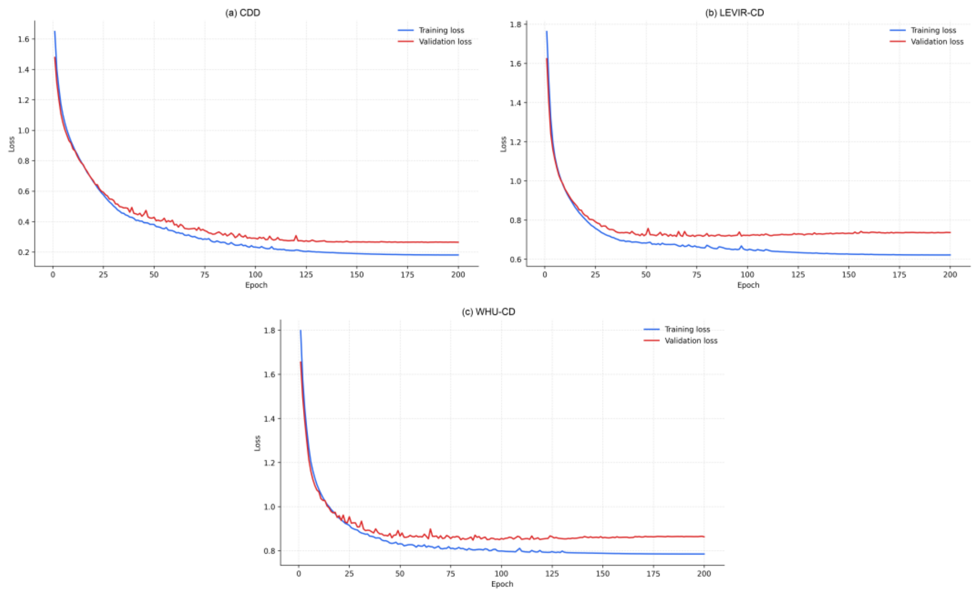
During model training, the validation F1 score was used as the criterion for model selection. Whenever a new best validation F1 score was achieved, the corresponding model checkpoint was saved. The checkpoint with the highest validation F1 score was subsequently used for testing. As shown in Figure 8, the best-performing models on the CDD (Figure 8a), LEVIR-CD (Figure 8b), and WHU-CD (Figure 8c) datasets were obtained at epochs 185, 93, and 134, respectively. As indicated by the loss curves, the training processes on all three datasets had entered relatively stable convergence stages at these epochs. For CDD, both the training and validation losses continued to decrease slowly during the later training stage; therefore, the optimal checkpoint appeared at the relatively late epoch of 185. For LEVIR-CD, the model completed its main feature-learning stage during the middle of training and achieved its highest validation F1 score at epoch 93. Although the training loss continued to decrease thereafter, the validation loss remained generally stable, and continued training did not yield better generalization performance. For WHU-CD, the highest validation F1 score was achieved at epoch 134, after which the validation loss and model performance generally stabilized. This model-selection strategy avoids the potential overfitting associated with directly using the parameters from the final epoch and ensures that the reported test results are obtained from the checkpoint exhibiting the best generalization performance on the validation set.
4.2. Comparative Results with Other Models
This section presents a comparative evaluation of the proposed GUF-Net against six remote sensing change detection models, including ChangeFormer [19], the Bi-temporal Image Transformer (BIT) [17], the Densely Connected Siamese Network (SNUNet) [52], the Ultra-Lightweight Spectral–Spatial Feature Collaboration Network (USSFC-Net) [18], the Multi-Scale Differential Feature Self-Attention Network (MDFA-Net) [35], and the Semantic-Aware Change Detection Network (SA-CDNet) [22]. In addition, for the experiments on the WHU-CD dataset, SA-CDNet integrated with the UACD uncertainty-aware framework (UACD–SA-CDNet) [24] is included as an additional comparison method to evaluate change detection performance and prediction reliability under uncertainty modeling. To ensure a fair comparison, all baseline models were retrained using the same training, validation, and test splits as GUF-Net and evaluated under the unified evaluation protocol described in Section 3.6.4.
Figure 8.
Loss curves of the model on three datasets.
- (1)
- Results on WHU-CD
As shown in Table 6, GUF-Net achieves competitive change detection performance on the WHU-CD dataset, ranking among the top three models across all evaluation metrics. In particular, its Precision reaches 96.07%, ranking second among all compared methods and indicating that the model effectively suppresses false detections in unchanged regions. Its Recall of 91.79% shows that most actual building-change regions can be successfully identified. By jointly considering Precision and Recall, GUF-Net obtains an F1 score of 93.88%, demonstrating a favorable balance between false detections and missed detections. Moreover, its IoU and OA reach 88.47% and 99.52%, respectively, indicating a high spatial overlap between the predicted change regions and ground-truth labels, as well as high overall pixel-classification accuracy.
Table 6.
Accuracy performance results of GUF-Net and comparison methods on WHU-CD dataset.
Compared with MDFA-Net, GUF-Net improves F1, Precision, Recall, IoU, and OA by 1.09, 0.57, 1.55, 1.91, and 0.08 percentage points, respectively. It also consistently outperforms ChangeFormer, BIT, SNUNet, and USSFC-Net across all five evaluation metrics. Compared with UACD-SA-CDNet, GUF-Net achieves a 0.13-percentage-point improvement in Precision, while its F1, Recall, IoU, and OA are lower by 0.36, 0.82, 0.65, and 0.03 percentage points, respectively. SA-CDNet achieves the best overall results, with F1 and IoU exceeding those of GUF-Net by 0.60 and 1.08 percentage points, whereas the differences in Precision and OA are only 0.10 and 0.05 percentage points. Overall, although GUF-Net does not obtain the highest values in the table, it maintains results close to the two leading models and outperforms the other five comparison methods, demonstrating the strong competitiveness of the proposed method on the WHU-CD dataset.
- (2)
- Results on CDD
As shown in Table 7, GUF-Net achieves strong overall detection performance on this dataset, with F1, Precision, Recall, IoU, and OA reaching 96.55%, 96.95%, 96.16%, 93.34%, and 99.15%, respectively. Among all compared models, GUF-Net obtains the highest F1, Precision, IoU, and OA, while ranking second in Recall, only 0.35 percentage points lower than USSFC-Net. The high Precision indicates that GUF-Net effectively reduces false detections in unchanged regions, while the Recall of 96.16% demonstrates that the model can identify most actual change regions. Overall, GUF-Net achieves a favorable balance between suppressing false detections and identifying change regions, while maintaining a high degree of spatial overlap between the predicted regions and the ground-truth labels.
Table 7.
Accuracy performance results of GUF-Net and comparison methods on CDD dataset.
Compared with USSFC-Net, which achieves relatively close overall performance, GUF-Net improves F1, Precision, IoU, and OA by 0.72, 1.78, 1.33, and 0.17 percentage points, respectively, although its Recall is 0.35 percentage points lower. This indicates that GUF-Net achieves better overall performance by reducing false detections while maintaining a high change-detection rate. Compared with MDFA-Net, GUF-Net improves F1, Recall, IoU, and OA by 1.98, 0.45, 3.64, and 0.48 percentage points, respectively. Compared with ChangeFormer, BIT, SNUNet, and SA-CDNet, GUF-Net likewise achieves higher F1, IoU, and OA.
- (3)
- Results on LEVIR-CD
As shown in Table 8, the evaluated models achieve relatively similar performance on this dataset. GUF-Net obtains an F1 score of 90.43%, a Precision of 91.72%, a Recall of 89.17%, an IoU of 82.53%, and an OA of 99.03%. Its relatively high Precision indicates that the model effectively suppresses false detections in unchanged regions, while the Recall of 89.17% demonstrates its ability to identify most actual change regions. GUF-Net ranks fourth in both F1 and IoU and ties with USSFC-Net for third place in OA, indicating that it achieves balanced and competitive detection performance on this dataset.
Table 8.
Accuracy performance results of GUF-Net and comparison methods on LEVIR-CD dataset.
SA-CDNet achieves the highest F1, IoU, and OA, reaching 90.77%, 83.10%, and 99.07%, respectively. USSFC-Net obtains the highest Precision of 92.15%, while ChangeFormer achieves the highest Recall of 90.18%. Compared with SA-CDNet, which delivers the best overall performance, GUF-Net is lower by only 0.34, 0.40, 0.28, 0.57, and 0.04 percentage points in F1, Precision, Recall, IoU, and OA, respectively, indicating a relatively small overall performance gap. Compared with USSFC-Net, GUF-Net improves F1, Recall, and IoU by 0.13, 0.64, and 0.20 percentage points, respectively, although its Precision is 0.43 percentage points lower; the two models achieve the same OA.
4.3. Ablation Experiments
This study proposes three core modules, namely DSDConv_DA, THFA, and GUF, and conducts progressive ablation experiments on the WHU-CD dataset to quantitatively analyze the contribution of each component. A non-weight-sharing Siamese U-Net is adopted as the baseline model. In addition, a GUF-NoU variant without Stage 4 uncertainty injection is introduced to distinguish the contribution of the gated fusion structure from that of the uncertainty information. As shown in Table 9, the baseline model achieves an F1 score of 89.51%. After introducing DSDConv_DA, the F1 score increases to 90.69%, while Precision and Recall reach 93.84% and 87.75%, respectively, demonstrating that this module improves the model’s feature extraction capability. With the further addition of THFA, the F1 score increases to 92.57%, Recall improves from 87.75% to 91.48%, and IoU reaches 86.16%, indicating that inter-temporal feature interaction contributes to more complete identification of change regions.
Table 9.
Accuracy performance results of core module ablation experiment of GUF-Net.
After introducing GUF-NoU, which excludes Stage 4 uncertainty injection, the F1 score increases to 92.99%, while Precision and Recall reach 94.23% and 91.78%, respectively. These results demonstrate that the gated feature fusion structure itself provides measurable performance gains. When the complete GUF module is employed, the F1 score further increases to 93.88%, representing an improvement of 0.89 percentage points over GUF-NoU. Precision increases from 94.23% to 96.07%, and IoU improves from 86.90% to 88.47%, while Recall remains nearly unchanged. These results indicate that injecting Stage 4 uncertainty information primarily enhances the model’s ability to suppress erroneous change responses, thereby reducing false detections and improving the spatial overlap between the predicted and ground-truth change regions.
The complete model ultimately achieves an F1 score of 93.88%, a Precision of 96.07%, a Recall of 91.79%, an IoU of 88.47%, and an OA of 99.52%, improving upon the baseline by 4.37, 4.01, 4.69, 7.45, and 0.33 percentage points, respectively. These results verify the effectiveness of combining the three proposed modules. The ablation variants were also subsequently evaluated under different noise conditions.
To investigate the contribution of each component in the redesigned loss function, additional loss-ablation experiments were conducted on the WHU-CD dataset while keeping the complete A4 network architecture, training settings, and random seed unchanged. As shown in Table 10, B0 adopts BCE + Dice; B1 replaces BCE with EDL-NLL; B2 further introduces the annealed KL regularization term with a maximum coefficient of 0.001; and B3 additionally applies Stage 4 auxiliary evidence supervision with a weight of 0.1. When BCE + Dice is used, the model achieves an F1 score of 92.89% and an IoU of 86.73%. Replacing BCE with EDL-NLL increases the F1 score and IoU to 93.03% and 86.97%, respectively. After introducing the annealed KL term, the F1 score, Precision, Recall, and IoU further increase to 93.62%, 94.74%, 92.53%, and 88.01%, respectively. With the addition of Stage 4 auxiliary evidence supervision, the F1 score, Precision, IoU, and OA further improve to 93.88%, 96.07%, 88.47%, and 99.52%, respectively, although Recall decreases from 92.53% to 91.79%. These results indicate that Stage 4 auxiliary supervision improves Precision and region-overlap performance, although coarse-scale supervision may introduce a trade-off in the detection of small changed regions, as reflected by the decrease in Recall.
Table 10.
Ablation study of the loss components and Stage 4 auxiliary supervision on WHU-CD.
4.4. Noise Experiment Results
To evaluate the robustness of the models under different noise disturbances, noise experiments were conducted on the WHU-CD test set by constructing three types of corrupted test sets: Gaussian noise, salt-and-pepper noise, and speckle noise. MDFA-Net, USSFC-Net, SA-CDNet, and UACD–SA-CDNet were selected for comparison. UACD [24] is a plug-and-play uncertainty-aware framework for change detection that estimates pixel-level predictive uncertainty through multiple stochastic predictions using MC Dropout and optimizes the model with an uncertainty-aware regularization term. UACD–SA-CDNet was included because it introduces explicit uncertainty estimation while retaining the basic SA-CDNet architecture, thereby enabling a comparison between GUF-Net and an existing uncertainty-aware method in terms of change detection performance and prediction reliability under noisy conditions. To ensure a fair comparison, all models used the same data split and noise settings. The noise-corrupted test sets were used exclusively for inference and evaluation and were not involved in model training or parameter tuning.
As shown in Figure 9 and Table 11, the change detection performance of almost all models decreases to varying degrees as the noise intensity increases, whereas GUF-Net exhibits more stable performance under all three types of noise. To quantify the actual image degradation caused by Gaussian noise, PSNR and SSIM were calculated between the corrupted and clean T1 images on the 744-pair WHU-CD test set. At σ = 0.03, 0.05, and 0.07, the average PSNR values were 30.47, 26.05, and 23.15 dB, respectively, while the corresponding SSIM values were 0.7945, 0.6251, and 0.4983. Under the strongest Gaussian, salt-and-pepper, and speckle noise conditions, GUF-Net achieves F1 scores of 93.02%, 89.93%, and 92.59%, respectively, corresponding to decreases of only 0.86, 3.95, and 1.29 percentage points relative to the clean images. Meanwhile, it maintains high Precision values, indicating its ability to suppress noise-induced false change responses. After incorporating uncertainty modeling, UACD-SA-CDNet shows improved stability over the original SA-CDNet under medium and high noise intensities. In particular, under the strongest Gaussian, salt-and-pepper, and speckle noise conditions, its F1 scores increase by 6.19, 8.61, and 4.82 percentage points, respectively, demonstrating that uncertainty information can partially alleviate noise-induced performance degradation. Nevertheless, under these three strongest noise conditions, the F1 scores of UACD-SA-CDNet remain 20.81, 19.58, and 46.94 percentage points lower than those of GUF-Net, respectively. Overall, incorporating uncertainty modeling alone improves the noise adaptability of SA-CDNet, whereas GUF-Net combines uncertainty estimation with gated feature fusion to maintain more stable change detection performance across different noise types and intensities, further demonstrating the noise robustness of the proposed model.
Figure 9.
Performance comparison of different models under three types of noise. The three columns from left to right present the results under Gaussian noise, salt-and-pepper noise, and speckle noise, respectively. The five rows from top to bottom represent the F1 score, precision, recall, IoU, and OA. Curves with different colors correspond to GUF-Net, USSFC-Net, MDFA-Net, SA-CDNet, and UACD-SA-CDNet.
Table 11.
F1 scores of different models under various noise conditions.
To further evaluate the performance stability of GUF-Net across different stochastic noise realizations, three independently corrupted test sets were generated for each noise condition using random seeds. The experiments were conducted under otherwise identical conditions, and the F1 results are reported as mean ± standard deviation. Under Gaussian noise with σ = 0.03, 0.05, and 0.07, the F1 scores are 93.77 ± 0.02%, 93.62 ± 0.06%, and 93.04 ± 0.10%, respectively. Under salt-and-pepper noise with densities of p = 0.01, 0.03, and 0.05, the corresponding F1 scores are 93.42 ± 0.07%, 92.15 ± 0.11%, and 89.79 ± 0.12%, respectively. Under speckle noise with σ = 0.05, 0.10, and 0.20, the F1 scores are 93.80 ± 0.04%, 93.67 ± 0.02%, and 92.66 ± 0.09%, respectively. The standard deviations remain below 0.12 percentage points under all conditions, indicating that GUF-Net exhibits a consistent performance trend across different stochastic noise realizations.
As shown in Figure 10, A2, A3, and A4 represent the model without the GUF module, the model employing GUF-NoU, and the model employing the complete GUF module, respectively. As the noise intensity increases, the performance of all three variants declines to varying degrees. Nevertheless, the complete model, A4, consistently achieves the highest F1 and IoU under Gaussian, salt-and-pepper, and speckle noise, while exhibiting more stable performance curves. Under the strongest levels of the three noise types, A4 achieves F1 scores of 93.02%, 89.93%, and 92.59%, corresponding to decreases of only 0.86, 3.95, and 1.29 percentage points relative to the clean test set. Compared with A3, these scores are higher by 1.85, 2.33, and 2.37 percentage points, respectively, and compared with A2, they are higher by 2.52, 17.72, and 10.69 percentage points, respectively.
Figure 10.
Performance comparison of different GUF-Net ablation variants under various noise types and intensities. The green, orange, and blue curves represent A4, A3, and A2, respectively. A2 denotes the model without the GUF module, A3 denotes the model employing GUF-NoU, and A4 denotes the model employing the complete GUF module. From left to right, the three columns correspond to Gaussian noise, salt-and-pepper noise, and speckle noise. From top to bottom, the five rows present F1, Precision, Recall, IoU, and OA as the noise intensity increases.
Under severe salt-and-pepper and speckle noise, A2 maintains relatively high Recall, but its Precision decreases to 60.34% and 75.01%, respectively, indicating that the model produces numerous noise-induced false change responses. After introducing GUF-NoU, A3 achieves substantial improvements in Precision, F1, and IoU, demonstrating that the gated fusion structure itself strengthens the model’s ability to suppress noise interference. Building on this structure, the complete GUF injects Stage 4 uncertainty information, enabling A4 to further increase its Precision to 96.57%, 91.66%, and 96.69% under the strongest Gaussian, salt-and-pepper, and speckle noise conditions, respectively, while also achieving higher F1, IoU, and OA. These results demonstrate that the gated fusion structure in GUF improves the model’s adaptability to noise, while the additional injection of uncertainty information helps identify and suppress noise-induced erroneous responses. Consequently, the complete model maintains more stable change detection performance across different noise types and intensities.
To determine whether the robustness improvement arises from the learned uncertainty information rather than from general feature scaling, we replaced the uncertainty map supplied to the GUF module with a mean-matched constant map, an independent uniform random map, and a spatially shuffled uncertainty map under the same experimental conditions. The corresponding results under clean and strongest-noise conditions are presented in Table 12.
Table 12.
F1 results of uncertainty-map substitution controls under clean and strongest-noise conditions.
As shown in Table 12, the model using the original uncertainty map exhibits the smallest F1 decrease under all three strongest-noise conditions. Under Gaussian noise with (σ = 0.07), the F1 scores of the original, constant, shuffled, and random uncertainty-map variants decrease by 0.86, 1.26, 0.94, and 1.25 percentage points, respectively, indicating relatively small differences among the variants. Under salt-and-pepper noise with (p = 0.05), the corresponding decreases are 3.95, 6.63, 11.42, and 19.67 percentage points, with spatial shuffling and random replacement causing substantially greater degradation. Under speckle noise with (σ = 0.20), the original uncertainty-map variant decreases by only 1.29 percentage points, whereas the constant, shuffled, and random variants decrease by 1.61, 6.32, and 5.72 percentage points, respectively. After spatially shuffling or randomly replacing the uncertainty map, the model exhibits greater performance degradation under strong salt-and-pepper and speckle noise, indicating that the spatial correspondence contained in the learned uncertainty map contributes to maintaining detection performance under noisy conditions. Meanwhile, the constant-map variant retains relatively strong performance under some noise conditions, suggesting that gate-based modulation and the overall uncertainty magnitude also contribute to the observed robustness. Therefore, the noise robustness of GUF-Net should not be attributed entirely to uncertainty injection, but rather to the combined effects of the modified encoder, global feature modeling, gated fusion structure, and pixel-level uncertainty information.
5. Discussion
This study proposed a GUF-Net based on a gating mechanism, which integrates CNN and Transformer feature extraction, explicit uncertainty modeling and fusion for BCD in remote sensing images. The following sections will elaborate on the model’s performance characteristics, methodological contributions, limitations, and future research directions.
GUF-Net achieves competitive performance across the three benchmark datasets, although it does not consistently rank first on every dataset. On WHU-CD, it obtains an F1 score of 93.88%, ranking third behind SA-CDNet (94.48%) and UACD-SA-CDNet (94.24%), while outperforming MDFA-Net (92.79%) and USSFC-Net (90.45%). On CDD, it achieves the highest F1 score of 96.55%, followed by USSFC-Net (95.83%) and MDFA-Net (94.57%). On LEVIR-CD, its F1 score is 90.43%, which is slightly lower than SA-CDNet (90.77%), MDFA-Net (90.71%), and ChangeFormer (90.50%). The average F1 score over the three datasets is 93.62%. These results indicate that GUF-Net has a reasonable overall accuracy, but its advantage is not uniform across different scenarios.
To further evaluate the performance stability of GUF-Net, three independent training and evaluation runs were conducted on the WHU-CD dataset using different random seeds. The results are reported as mean ± standard deviation. GUF-Net achieves an F1 score of 93.50 ± 0.34%, Precision of 94.98 ± 0.97%, Recall of 92.06 ± 0.27%, IoU of 87.78 ± 0.61%, and OA of 99.49 ± 0.03%. The relatively small standard deviations, particularly for F1 and OA, indicate that GUF-Net maintains reasonably consistent overall performance across different training random seeds on WHU-CD.
The robustness of GUF-Net was further evaluated under three simulated noise types on the WHU-CD test set. Under the strongest Gaussian noise (σ = 0.07), the F1 score of GUF-Net decreases from 93.88% to 93.02%, a drop of 0.86 percentage points; under salt-and-pepper noise (p = 0.05), the F1 score drops by 3.95 percentage points to 89.93%; under speckle noise (σ = 0.20), the F1 score drops by 1.29 percentage points to 92.59%. These F1 values are 1.60, 5.67, and 5.80 percentage points higher than the second-best compared model under the corresponding noise conditions. This suggests that GUF-Net is relatively less affected by the tested noise types. Visual inspection of Figure 11 shows that in relatively clean scenes the detection results remain largely stable, while in more complex scenes noise causes fragmented change-probability responses and increased missed detections. In addition, high-uncertainty regions in the uncertainty maps exhibit a spatial correspondence with erroneous predictions, indicating that the estimated uncertainty can to some extent reflect prediction reliability under noisy conditions.
Figure 11.
Change detection and uncertainty visualization results of GUF-Net under clean and different noisy conditions. From left to right, the columns show the T1 image, T2 image, (a) ground truth, (b) error-type map, (c) change-probability map, (d) pixel-level uncertainty map, and (e) uncertainty heatmap. Rows 1–4 and Rows 5–8 correspond to two different scenes, respectively. For each scene, the results are presented under clean, Gaussian-noise, salt-and-pepper-noise, and speckle-noise conditions in sequence.
As shown in Figure 11, the samples presented are representative examples selected for qualitative illustration. From left to right, the columns show the T1 image, T2 image, ground truth, error-type map, change-probability map, pixel-level uncertainty map, and uncertainty heatmap. T1 is the noise-corrupted temporal image, whereas T2 and the ground-truth label remain unchanged across all noise conditions. In the error-type map, white, black, red, and green represent true positives, true negatives, false positives, and false negatives, respectively. Brighter pixels in the change-probability map indicate higher probabilities of belonging to the changed class, while brighter regions in the uncertainty map indicate greater model uncertainty. The heatmap colorizes the uncertainty values using a shared global normalization scale, where blue and red represent relatively low and high uncertainty, respectively.
Rows 1–4 correspond to the first scene and sequentially present the detection results under clean, Gaussian-noise, salt-and-pepper-noise, and speckle-noise conditions. The building boundaries in this scene are relatively clear. After introducing different types of noise, the change-probability responses and detection results for the main building regions remain largely stable. The error-type maps are still dominated by white true-positive and black true-negative pixels, with only a small number of red false-positive and green false-negative pixels appearing along the building boundaries. This indicates that the model exhibits good noise robustness in this type of scene. Meanwhile, relatively high uncertainty is mainly concentrated around building boundaries and a small number of incorrectly predicted regions.
Rows 5–8 present the results for the second, more complex scene in the same order. Under the clean condition in Row 5, the model identifies the main changed buildings relatively completely. After Gaussian noise is introduced in Row 6, the main building regions remain detectable, although missed detections begin to appear in some local areas. In Row 7, salt-and-pepper noise causes the change-probability responses to become more fragmented, with a noticeable increase in green false-negative pixels within the buildings. In Row 8, speckle noise further interferes with building textures and boundaries, resulting in enlarged missed-detection regions. Corresponding to these prediction errors, the high-response regions in the uncertainty maps and heatmaps gradually increase from Rows 6 to 8 and are mainly distributed over building boundaries, noise-disturbed texture regions, and false-positive or false-negative areas.
These results demonstrate that the model can retain its ability to detect the principal change regions under noisy conditions. When noise degrades prediction performance, the model’s estimated uncertainty also increases accordingly and exhibits a clear spatial correspondence with erroneous regions, demonstrating the model’s ability to identify potentially unreliable predictions.
To quantitatively analyze the relationship between pixel-level uncertainty and prediction errors, the Area Under the Receiver Operating Characteristic Curve (AUROC) is adopted as the error-detection metric. Incorrectly predicted pixels are defined as positive samples, correctly predicted pixels as negative samples, and pixel-level uncertainty as the error-detection score. The true-positive and false-positive rates are calculated by varying the uncertainty threshold to generate the ROC curve. An AUROC closer to 1 indicates a stronger ability to distinguish incorrectly predicted pixels, whereas an AUROC of 0.5 corresponds to random detection.
As shown in Figure 12, the model achieves AUROC values of 0.7195, 0.6989, 0.7112, and 0.6942 under clean, Gaussian-noise, salt-and-pepper-noise, and speckle-noise conditions, respectively, all exceeding the random-detection level. These results indicate that incorrectly predicted pixels generally exhibit higher uncertainty and that the estimated uncertainty reflects pixel-level prediction reliability. Moreover, the AUROC remains above 0.69 under all three noise conditions, demonstrating that the uncertainty representation retains relatively stable error-awareness capability under different noise disturbances.
Figure 12.
Uncertainty-based pixel-error detection under clean and noisy conditions.
To further examine the actual influence of the Stage 4 uncertainty map entering the GUF module on the prediction results, we kept all parameters of the complete model fixed and replaced only the uncertainty map during inference with a mean-matched constant map, a spatially shuffled map, or an all-zero map. Unlike the experiments in Table 12, in which each substitution variant was trained and evaluated separately, this analysis examines the pixel-level prediction changes produced by altering the uncertainty input of the same trained model. With the learned uncertainty map, the model achieved an F1 score of 93.88% and an IoU of 88.47%. Replacing it with the constant, shuffled, and zero maps reduced the F1 score to 93.61%, 93.60%, and 92.01%, respectively, and the IoU to 88.00%, 87.96%, and 85.20%, respectively.
Pixels that were incorrectly predicted under an intervention but correctly predicted when using the learned uncertainty map were defined as corrected pixels, whereas the opposite cases were defined as introduced errors. After subtracting the introduced errors, the learned uncertainty map produced net reductions of 8503, 9142, and 61,844 erroneous pixels relative to the constant-map, shuffled-map, and zero-map interventions, respectively. The pixels were further divided into five equal-sized groups according to their Stage 4 uncertainty. Relative to the zero-map intervention, the error-correction rate increased from 1.17% in the lowest-uncertainty group to 35.42% in the highest-uncertainty group, and approximately 90% of the net error reduction occurred among the 20% of pixels with the highest uncertainty.
In addition, the Stage 4 uncertainty entering GUF achieved an AUROC of 0.8401 for pixel-wise error detection, whereas the uncertainty derived from the final output head achieved an AUROC of 0.7195. The former is used to modulate deep features within GUF, whereas the latter is derived from the evidence produced after gated fusion and multi-stage decoding. Therefore, these values do not represent a direct before-and-after comparison of the same uncertainty map. Based on the intervention results, the relatively lower AUROC of the final-output uncertainty may be associated with the correction of some high-uncertainty errors during fusion and a weakened correspondence between the remaining errors and the uncertainty scores. Overall, these results indicate that the learned Stage 4 uncertainty has a relatively strong correspondence with error-prone regions and that its contribution is concentrated primarily in highly uncertain areas. Nevertheless, the overall model performance remains attributable to the combined effects of the gating structure, feature representation, overall uncertainty magnitude, and spatial uncertainty information.
To evaluate the calibration of the final change probabilities using a common metric, the Expected Calibration Error (ECE) was calculated for GUF-Net and UACD-SA-CDNet on the same WHU-CD test set. For both models, ECE was computed from the final change probabilities using 15 equal-width confidence bins, with a lower ECE indicating a smaller overall discrepancy between prediction confidence and empirical accuracy. Under the clean condition, UACD-SA-CDNet and GUF-Net achieve ECE values of 0.0968% and 0.2336%, respectively, indicating better probability calibration for the former. However, under the strongest Gaussian, salt-and-pepper, and speckle noise conditions, the ECE values of UACD-SA-CDNet increase to 0.9927%, 1.8184%, and 6.4549%, respectively, whereas those of GUF-Net are 0.1676%, 0.1039%, and 0.1624%. These results indicate that the final change probabilities produced by GUF-Net exhibit more stable overall calibration errors under strong noise conditions.
GUF-Net contributes to BCD under noisy conditions mainly in two aspects. First, the Stage 4 uncertainty map corresponds spatially to prediction errors; injecting it into the gated fusion (GUF vs. GUF-NoU) improves F1 by 1.85, 2.33, and 2.37 percentage points under the strongest Gaussian, salt-and-pepper, and speckle noise, while recall changes little, indicating that uncertainty mainly helps suppress noise-induced false changes. Second, the gated fusion structure itself contributes to robustness: under severe salt-and-pepper and speckle noise, the gated fusion without uncertainty (GUF-NoU) markedly improves precision, F1, and IoU over the model without the GUF module. THFA serves as a supporting global-context extractor and is associated with improved recall; however, the A2 variant retains relatively high recall under noise while its Precision decreases to 60.34% and 75.01% under severe salt-and-pepper and speckle noise, respectively. These observations suggest that global context alone is insufficient for controlling noise-induced false responses, whereas gated fusion and uncertainty injection provide the main benefits for precision retention.
Despite its strong robustness under simulated noise, GUF-Net has several limitations that should be acknowledged. First, on clean benchmarks GUF-Net does not consistently achieve the best metrics across all datasets and all indicators. The results suggest that the accuracy advantage of GUF-Net is not uniform across datasets; the gating and uncertainty mechanisms mainly contribute to robustness under noise, whereas on clean, sparsely changed benchmarks such as LEVIR-CD they do not provide consistent gains over methods directly optimized for clean-set accuracy. This is mainly because GUF-Net prioritizes uncertainty quantification and noise robustness rather than maximizing clean-set accuracy. The encoder relies on DSDConv_DA to remain lightweight and multi-scale; however, DSDConv may weaken fine-grained spectral discrimination compared with heavier full convolutions, and the dilated branches can introduce boundary blurring for small or irregular buildings. In addition, the Stage 4 uncertainty head, uncertainty branch, and THFA global aggregation consume model capacity that would otherwise be used for pure change-classification refinement. On idealized, low-noise datasets, the gating and uncertainty suppression mechanisms provide limited gains, while their regularization effect may slightly reduce over-confident predictions and hence marginally lower precision/recall trade-offs relative to models specifically optimized for clean accuracy.
Second, the current evaluation is limited to RGB optical images and three types of synthetic noise. All experiments use WHU-CD, CDD, and LEVIR-CD, which provide only RGB bands; no multispectral or SAR data are tested. Our noise protocol only simulated Gaussian, salt-and-pepper, and speckle noise, but does not cover real-world degradations such as sensor thermal and photon noise, atmospheric scattering, illumination/seasonal changes, cloud shadows, misregistration, or compression artifacts. Moreover, all tests are conducted on fixed-size benchmark tiles; we do not evaluate large-scale mosaic images, cross-city generalization, or operational scenarios with limited annotations. Therefore, the reported noise robustness may not fully predict performance in real acquisition conditions.
Third, as shown in Table 13, GUF-Net has a relatively large parameter count of 86.271 M, with 116.720 GFLOPs, 57.93 pairs/s, and 17.26 ms/pair. In comparison, USSFC-Net is the most lightweight and fastest (1.519 M parameters, 9.720 GFLOPs, 75.84 pairs/s), followed by MDFA-Net (37.068 M parameters, 31.779 GFLOPs, 56.77 pairs/s). UACD-SA-CDNet has the highest FLOPs (253.351 GFLOPs) and the lowest throughput (13.57 pairs/s) among the compared models. The relatively large parameter count of GUF-Net mainly comes from the THFA Transformer blocks, the dual-channel uncertainty head at Stage 4, and the gated fusion of features and uncertainty maps in the decoder. For large-scene images, inference may require tiling with overlapping patches and subsequent stitching, which increases memory consumption and latency. Therefore, further reducing the model size and computational complexity, e.g., through compression or distillation, remains an important direction for future work.
Table 13.
Comparison of model complexity and inference efficiency on the WHU-CD dataset.
Correspondingly, future work could focus on three aspects. First, to improve clean-set accuracy while retaining noise robustness, we will explore adaptive training strategies that balance uncertainty regularization and classification gains, and develop more efficient multi-scale feature extraction modules to mitigate boundary blurring. Second, we will extend validation to multispectral and SAR data, real-world degradation conditions such as atmospheric effects, cloud shadows, and misregistration, as well as large-scale cross-city scenarios, enabling evaluation under operational acquisition settings. Third, to address the computational overhead, we will investigate knowledge distillation, pruning, quantization, and more efficient Transformer designs, together with tiling-based inference strategies for very large images with lower memory and latency.
6. Conclusions
In this paper, we presented GUF-Net, a gated uncertainty fusion architecture designed to address the challenges of insufficient feature fusion and noise interference in building change detection. The model explicitly quantifies pixel-level uncertainty through a dual-channel output of change probability and uncertainty value, and adaptively fuses multi-scale features with uncertainty maps via a dynamic gating mechanism. In addition, the loss function is redesigned to directly supervise the uncertainty estimation, ensuring that it genuinely reflects prediction reliability rather than serving as an unsupervised auxiliary output. Distinct from prior uncertainty-aware detectors that rely on unsupervised auxiliary cues and static reweighting, GUF-Net tightly couples supervised evidential uncertainty with adaptive gating. On three clean public benchmarks, GUF-Net achieves competitive F1 scores of 93.88%, 96.55%, and 90.43% on WHU-CD, CDD, and LEVIR-CD, respectively, demonstrating comparable overall accuracy. Although it does not achieve the best result on every clean dataset, it exhibited the smallest F1 decrease at the highest tested level of each noise type. Under the strongest Gaussian, salt-and-pepper, and speckle noise on the WHU-CD test set, the F1 score drops by only 0.86, 3.95, and 1.29 percentage points, respectively, considerably smaller than the degradation of the compared models, demonstrating its robustness in diverse simulated noisy environments. Ablation studies confirm that the gated fusion module, the uncertainty injection, and the global context aggregation each contribute to the overall accuracy and noise resistance. While the model does not consistently outperform all methods on every dataset, the explicit uncertainty modeling and adaptive fusion provide a reliable mechanism for handling noise and complex scenes. Future work will focus on improving clean-set accuracy on challenging benchmarks, extending the evaluation to multispectral and SAR data, and reducing the computational cost for practical deployment.
Author Contributions
Conceptualization, S.Z. and Y.L. (Yuanling Li); methodology, J.Z., S.Z. and Y.L. (Yuanling Li); investigation, Y.L. (Yun Li); resources, Y.L. (Yuanling Li) and Y.L. (Yun Li); data curation, Y.L. (Yuanling Li); writing—original draft, J.Z. and Y.L. (Yuanling Li); writing—review and editing, J.Z. and S.Z.; visualization, J.Z. and Y.L. (Yuanling Li); supervision, S.Z. and Y.L. (Yun Li); project administration, Y.L. (Yun Li); funding acquisition, S.Z. All authors have read and agreed to the published version of the manuscript.
Funding
This research was funded by National Natural Science Foundation of China grant number 42501233 and Beijing Forestry University grant number BLX202363.
Data Availability Statement
All three datasets, LEVIR-CD, WHU-CD, and CDD, are open-access. LEVIR-CD: https://justchenhao.github.io/LEVIR/ (10 August 2026); WHU-CD: http://gpcv.whu.edu.cn/data/building_dataset.html (10 August 2026); CDD: https://zenodo.org/records/13290067 (10 August 2026).
Conflicts of Interest
The authors declare no conflicts of interest.
References
- Radke, R.J.; Andra, S.; Al-Kofahi, O.; Roysam, B. Image change detection algorithms: A systematic survey. IEEE Trans. Image Process. 2005, 14, 294–307. [Google Scholar] [CrossRef] [Scilit] [PubMed]
- Chen, S.; Shi, W.; Zhou, M.; Zhang, M.; Yu, Y.; Sun, Y.; Guan, L.; Li, S. CDasXORNet: Change detection of buildings from bi-temporal remote sensing images as an XOR problem. Int. J. Appl. Earth Obs. Geoinf. 2024, 130, 103836. [Google Scholar] [CrossRef] [Scilit]
- Zheng, Z.; Zhong, Y.; Wang, J.; Ma, A.; Zhang, L. Building damage assessment for rapid disaster response with a deep object-based semantic change detection framework: From natural disasters to man-made disasters. Remote Sens. Environ. 2021, 265, 112636. [Google Scholar] [CrossRef] [Scilit]
- Khankeshizadeh, E.; Mohammadzadeh, A.; Mohsenifar, A.; Moghimi, A.; Pirasteh, S.; Feng, S.; Hu, K.; Li, J. Building detection in VHR remote sensing images using a novel dual attention residual-based U-Net (DAttResU-Net): An application to generating building change maps. Remote Sens. Appl. Soc. Environ. 2024, 36, 101336. [Google Scholar] [CrossRef] [Scilit]
- Wu, J.; Ni, W.; Bian, H.; Cheng, K.; Liu, Q.; Kong, X.; Li, B. Unsupervised Change Detection for VHR Remote Sensing Images Based on Temporal-Spatial-Structural Graphs. Remote Sens. 2023, 15, 1770. [Google Scholar] [CrossRef] [Scilit]
- Chen, H.; Shi, Z. A spatial-temporal attention-based method and a new dataset for remote sensing image change detection. Remote Sens. 2020, 12, 1662. [Google Scholar] [CrossRef] [Scilit]
- Li, J.; He, W.; Li, Z.; Guo, Y.; Zhang, H. Overcoming the uncertainty challenges in detecting building changes from remote sensing images. ISPRS J. Photogramm. Remote Sens. 2025, 220, 1–17. [Google Scholar] [CrossRef] [Scilit]
- Song, A.; Kim, Y.; Han, Y. Uncertainty analysis for object-based change detection in very high-resolution satellite images using deep learning network. Remote Sens. 2020, 12, 2345. [Google Scholar] [CrossRef] [Scilit]
- Hussain, M.; Chen, D.; Cheng, A.; Wei, H.; Stanley, D. Change detection from remotely sensed images: From pixel-based to object-based approaches. ISPRS J. Photogramm. Remote Sens. 2013, 80, 91–106. [Google Scholar] [CrossRef] [Scilit]
- Quarmby, N.; Cushnie, J. Monitoring urban land cover changes at the urban fringe from SPOT HRV imagery in south-east England. Int. J. Remote Sens. 1989, 10, 953–963. [Google Scholar] [CrossRef] [Scilit]
- Du, S.; Li, W.; Li, J.; Du, S.; Zhang, C.; Sun, Y. Open-pit mine change detection from high resolution remote sensing images using DA-UNet++ and object-based approach. Int. J. Min. Reclam. Environ. 2022, 36, 512–535. [Google Scholar] [CrossRef] [Scilit]
- Huang, L.; Zhang, G.; Li, Y. An object-based change detection approach by integrating intensity and texture differences. In Proceedings of the 2010 2nd International Asia Conference on Informatics in Control, Automation and Robotics (CAR 2010), Wuhan, China, 6–7 March 2010; pp. 258–261. [Google Scholar]
- Gong, M.; Zhao, J.; Liu, J.; Miao, Q.; Jiao, L. Change detection in synthetic aperture radar images based on deep neural networks. IEEE Trans. Neural Netw. Learn. Syst. 2015, 27, 125–138. [Google Scholar] [CrossRef] [Scilit] [PubMed]
- Chen, P.; Zhang, B.; Hong, D.; Chen, Z.; Yang, X.; Li, B. FCCDN: Feature constraint network for VHR image change detection. ISPRS J. Photogramm. Remote Sens. 2022, 187, 101–119. [Google Scholar] [CrossRef] [Scilit]
- Peng, X.; Zhong, R.; Li, Z.; Li, Q. Optical remote sensing image change detection based on attention mechanism and image difference. IEEE Trans. Geosci. Remote Sens. 2020, 59, 7296–7307. [Google Scholar] [CrossRef] [Scilit]
- Zhang, C.; Yue, P.; Tapete, D.; Jiang, L.; Shangguan, B.; Huang, L.; Liu, G. A deeply supervised image fusion network for change detection in high resolution bi-temporal remote sensing images. ISPRS J. Photogramm. Remote Sens. 2020, 166, 183–200. [Google Scholar] [CrossRef] [Scilit]
- Chen, H.; Qi, Z.; Shi, Z. Remote sensing image change detection with transformers. IEEE Trans. Geosci. Remote Sens. 2021, 60, 5607514. [Google Scholar] [CrossRef] [Scilit]
- Lei, T.; Geng, X.; Ning, H.; Lv, Z.; Gong, M.; Jin, Y.; Nandi, A.K. Ultralightweight spatial–spectral feature cooperation network for change detection in remote sensing images. IEEE Trans. Geosci. Remote Sens. 2023, 61, 4402114. [Google Scholar] [CrossRef] [Scilit]
- Bandara, W.G.C.; Patel, V.M. A transformer-based siamese network for change detection. In Proceedings of the IGARSS 2022-2022 IEEE International Geoscience and Remote Sensing Symposium, Kuala Lumpur, Malaysia, 17–22 July 2022; pp. 207–210. [Google Scholar]
- Xu, Y.; Wu, L.; Liu, X.; Chen, C.; Li, Y.; Zhang, Q.; Liu, M.; Zhang, T.; Yang, B. Remote sensing change detection method based on dynamic adaptive focal loss. IEEE Trans. Geosci. Remote Sens. 2024, 62, 5621515. [Google Scholar] [CrossRef] [Scilit]
- Yu, W.; Zhuo, L.; Li, J. GCFormer: Global context-aware transformer for remote sensing image change detection. IEEE Trans. Geosci. Remote Sens. 2024, 62, 4703212. [Google Scholar] [CrossRef] [Scilit]
- Gan, Y.; Xuan, W.; Luo, Z.; Fang, L.; Wang, Z.; Liu, J.; Du, B. Detect Changes Like Humans: Incorporating Semantic Priors for Improved Change Detection. IEEE Trans. Geosci. Remote Sens. 2025, 63, 4417414. [Google Scholar] [CrossRef] [Scilit]
- Di, Z.; Zhang, M.; Jiang, F.; Zhou, Y.; Gong, M. A General Uncertainty-Guided Bayesian Adaptation Framework for Building Change Detection. IEEE Trans. Geosci. Remote Sens. 2025, 63, 5651414. [Google Scholar] [CrossRef] [Scilit]
- Gan, Y.; Li, Y.; Xuan, W.; Fang, L.; Liu, J.; Du, B. UACD: A Plug-and-play Framework for Uncertainty-aware Change Detection. IEEE Geosci. Remote Sens. Lett. 2026, 23, 6013105. [Google Scholar] [CrossRef] [Scilit]
- Jing, W.; Chi, K.; Li, Q.; Wang, Q. ChangeRD: A registration-integrated change detection framework for unaligned remote sensing images. ISPRS J. Photogramm. Remote Sens. 2025, 220, 64–74. [Google Scholar] [CrossRef] [Scilit]
- Xia, L.; Chen, J.; Luo, J.; Zhang, J.; Yang, D.; Shen, Z. Building change detection based on an edge-guided convolutional neural network combined with a transformer. Remote Sens. 2022, 14, 4524. [Google Scholar] [CrossRef] [Scilit]
- Lei, T.; Xu, Y.; Ning, H.; Lv, Z.; Min, C.; Jin, Y.; Nandi, A.K. Lightweight structure-aware transformer network for remote sensing image change detection. IEEE Geosci. Remote Sens. Lett. 2023, 21, 6000305. [Google Scholar] [CrossRef] [Scilit]
- Chen, M.; Zhang, Q.; Ge, X.; Xu, B.; Hu, H.; Zhu, Q.; Zhang, X. A full-scale connected CNN–transformer network for remote sensing image change detection. Remote Sens. 2023, 15, 5383. [Google Scholar] [CrossRef] [Scilit]
- Chen, H.; Song, J.; Han, C.; Xia, J.; Yokoya, N. ChangeMamba: Remote sensing change detection with spatiotemporal state space model. IEEE Trans. Geosci. Remote Sens. 2024, 62, 4409720. [Google Scholar] [CrossRef] [Scilit]
- Blundell, C.; Cornebise, J.; Kavukcuoglu, K.; Wierstra, D. Weight uncertainty in neural network. In Proceedings of the International Conference on Machine Learning, Lilie, France, 6–11 July 2015; pp. 1613–1622. [Google Scholar]
- Yang, Y.; Tang, X.; Ma, J.; Zhang, X.; Pei, S.; Jiao, L. ECPS: Cross pseudo supervision based on ensemble learning for semi-supervised remote sensing change detection. IEEE Trans. Geosci. Remote Sens. 2024, 62, 5612317. [Google Scholar] [CrossRef] [Scilit]
- Chen, H.; Li, W.; Shi, Z. Adversarial instance augmentation for building change detection in remote sensing images. IEEE Trans. Geosci. Remote Sens. 2021, 60, 5603216. [Google Scholar] [CrossRef] [Scilit]
- Kendall, A.; Gal, Y. What uncertainties do we need in bayesian deep learning for computer vision? In Advances in Neural Information Processing Systems 30 (NIPS 2017); Curran Associates, Inc.: Red Hook, NY, USA, 2017; Volume 30, pp. 1–11. [Google Scholar]
- Woo, S.; Park, J.; Lee, J.-Y.; Kweon, I.S. CBAM: Convolutional Block Attention Module. In Proceedings of the Computer Vision—ECCV 2018, Cham, Switzerland, 8–14 September 2018; pp. 3–19. [Google Scholar]
- Li, Y.; Zou, S.; Zhao, T.; Su, X. MDFA-Net: Multi-scale differential feature self-attention network for building change detection in remote sensing images. Remote Sens. 2024, 16, 3466. [Google Scholar] [CrossRef] [Scilit]
- Fu, Z.; Li, J.; Ren, L.; Chen, Z. SLDDNet: Stagewise short and long distance dependency network for remote sensing change detection. IEEE Trans. Geosci. Remote Sens. 2023, 61, 3000319. [Google Scholar] [CrossRef] [Scilit]
- Zhang, K.; Zhao, X.; Zhang, F.; Ding, L.; Sun, J.; Bruzzone, L. Relation changes matter: Cross-temporal difference transformer for change detection in remote sensing images. IEEE Trans. Geosci. Remote Sens. 2023, 61, 5611615. [Google Scholar] [CrossRef] [Scilit]
- Lobacheva, E.; Chirkova, N.; Kodryan, M.; Vetrov, D.P. On power laws in deep ensembles. Adv. Neural Inf. Process. Syst. 2020, 33, 2375–2385. [Google Scholar]
- Lu, P.; Ding, H.; Tian, X. DFANet: A deep feature attention network for building change detection in remote sensing imagery. Remote Sens. 2025, 17, 2575. [Google Scholar] [CrossRef] [Scilit]
- Wang, Y.; Wang, M.; Hao, Z.; Wang, Q.; Wang, Q.; Ye, Y. Msgfnet: Multi-scale gated fusion network for remote sensing image change detection. Remote Sens. 2024, 16, 572. [Google Scholar] [CrossRef] [Scilit]
- Zhang, X.; Chen, H.; Zhao, Y.; He, M.; Han, X. Change detection of buildings in remote sensing images using a spatially and contextually aware Siamese network. Expert Syst. Appl. 2025, 276, 127110. [Google Scholar] [CrossRef] [Scilit]
- Deng, J.; Gong, G.; Zhou, G.; Yan, M.; Li, L. A gated feature fusion network with meta-encoder and self-calibrating cross module for building change detection in remote sensing images. IEEE Trans. Geosci. Remote Sens. 2024, 62, 4709416. [Google Scholar] [CrossRef] [Scilit]
- Sensoy, M.; Kaplan, L.; Kandemir, M. Evidential deep learning to quantify classification uncertainty. In Advances in Neural Information Processing Systems 31 (NIPS 2018); Curran Associates, Inc.: Red Hook, NY, USA, 2018; Volume 31, pp. 1–11. [Google Scholar]
- Sudre, C.H.; Li, W.; Vercauteren, T.; Ourselin, S.; Jorge Cardoso, M. Generalised dice overlap as a deep learning loss function for highly unbalanced segmentations. In Proceedings of the International Workshop on Deep Learning in Medical Image Analysis, Quebec, QC, Canada, 14 September 2017; pp. 240–248. [Google Scholar]
- Ji, S.; Wei, S.; Lu, M. Fully convolutional networks for multisource building extraction from an open aerial and satellite imagery data set. IEEE Trans. Geosci. Remote Sens. 2018, 57, 574–586. [Google Scholar] [CrossRef] [Scilit]
- Lebedev, M.; Vizilter, Y.V.; Vygolov, O.; Knyaz, V.A.; Rubis, A.Y. Change detection in remote sensing images using conditional adversarial networks. Int. Arch. Photogramm. Remote Sens. Spat. Inf. Sci. 2018, 42, 565–571. [Google Scholar] [CrossRef] [Scilit]
- Hassouna, A.A.A.; Ismail, M.B.; Alqahtani, A.; Alqahtani, N.; Hassan, A.S.; Ashqar, H.I.; AlSobeh, A.M.; Hassan, A.A.; Elhenawy, M. A Generic and Extendable Framework for Benchmarking and Assessing the Change Detection Models. Preprints 2024. [Google Scholar] [CrossRef] [Scilit]
- Wang, Y.; Makrogiannis, S.; Kambhamettu, C. FAF-CD: Frequency-Aware Fusion for Change Detection under Imperfect Multimodal Remote Sensing. arXiv 2026, arXiv:2606.03114. [Google Scholar]
- Zhang, K.; Zuo, W.; Chen, Y.; Meng, D.; Zhang, L. Beyond a gaussian denoiser: Residual learning of deep cnn for image denoising. IEEE Trans. Image Process. 2017, 26, 3142–3155. [Google Scholar] [CrossRef] [Scilit] [PubMed]
- Chan, R.H.; Ho, C.-W.; Nikolova, M. Salt-and-pepper noise removal by median-type noise detectors and detail-preserving regularization. IEEE Trans. Image Process. 2005, 14, 1479–1485. [Google Scholar] [CrossRef] [Scilit] [PubMed]
- Lee, J.-S. Speckle analysis and smoothing of synthetic aperture radar images. Comput. Graph. Image Process. 1981, 17, 24–32. [Google Scholar] [CrossRef] [Scilit]
- Fang, S.; Li, K.; Shao, J.; Li, Z. SNUNet-CD: A densely connected Siamese network for change detection of VHR images. IEEE Geosci. Remote Sens. Lett. 2021, 19, 8007805. [Google Scholar] [CrossRef] [Scilit]
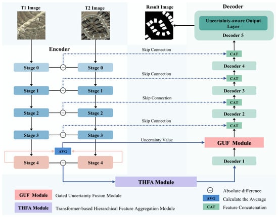
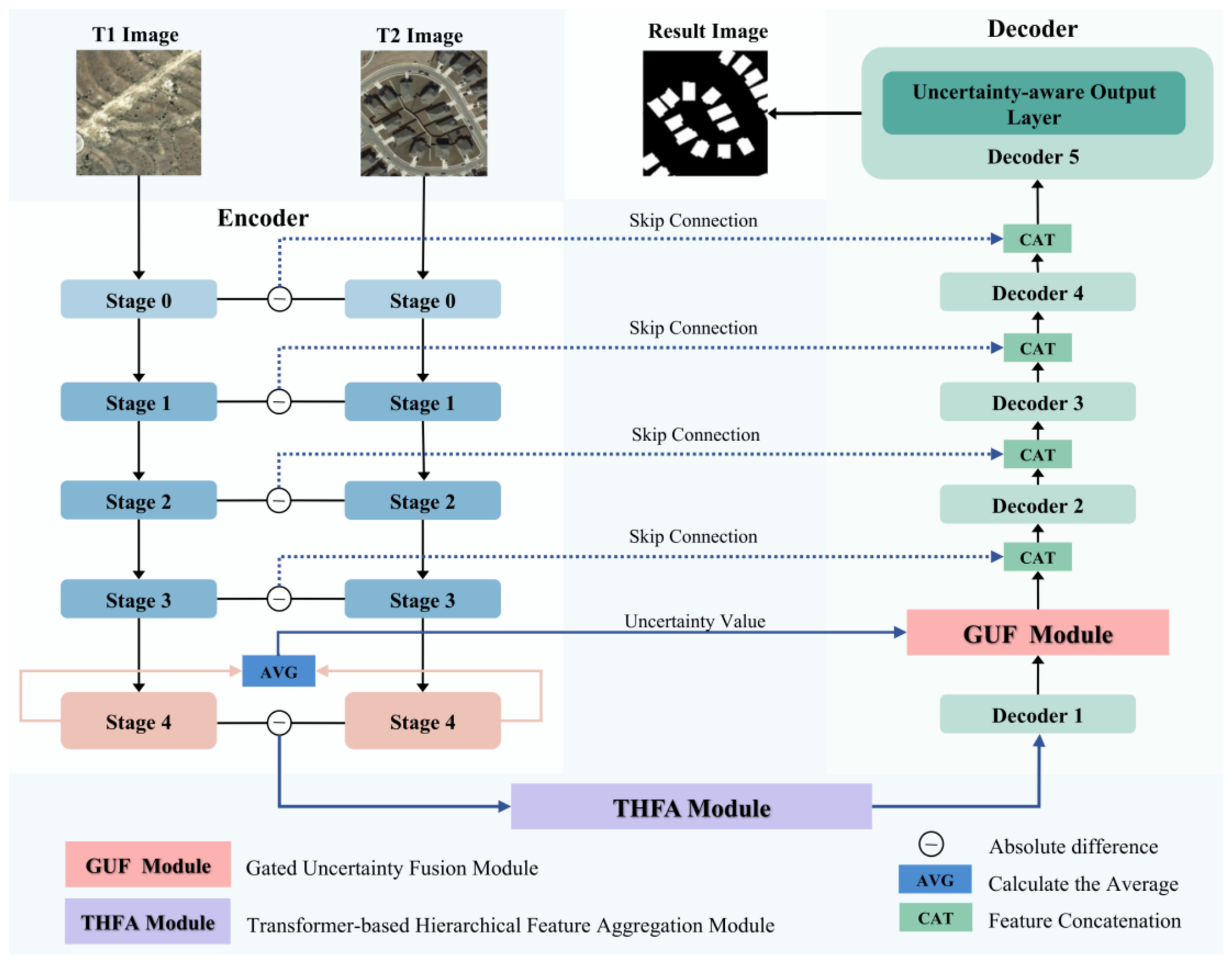
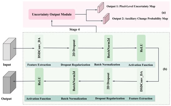
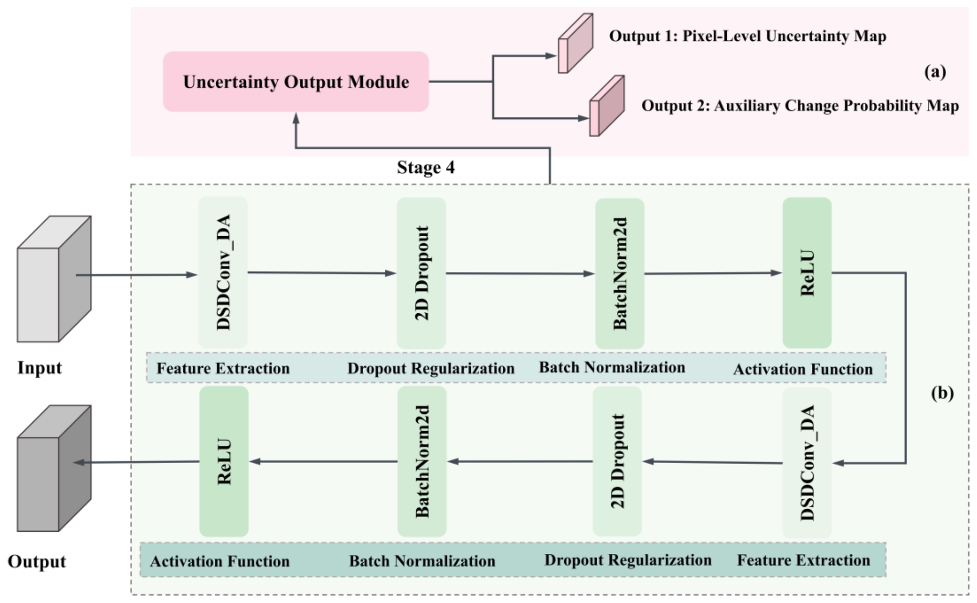
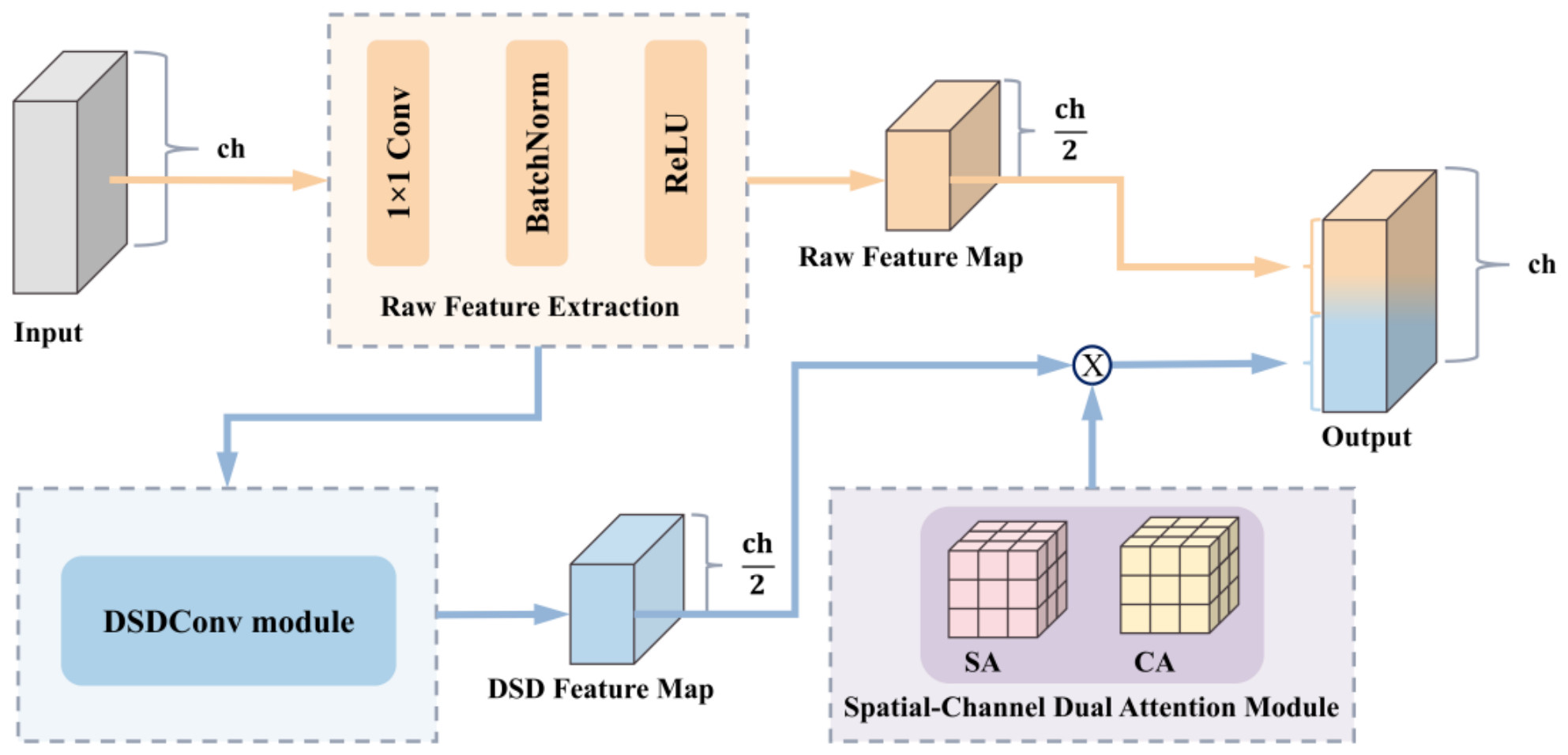
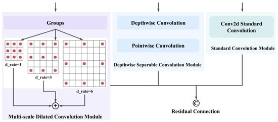
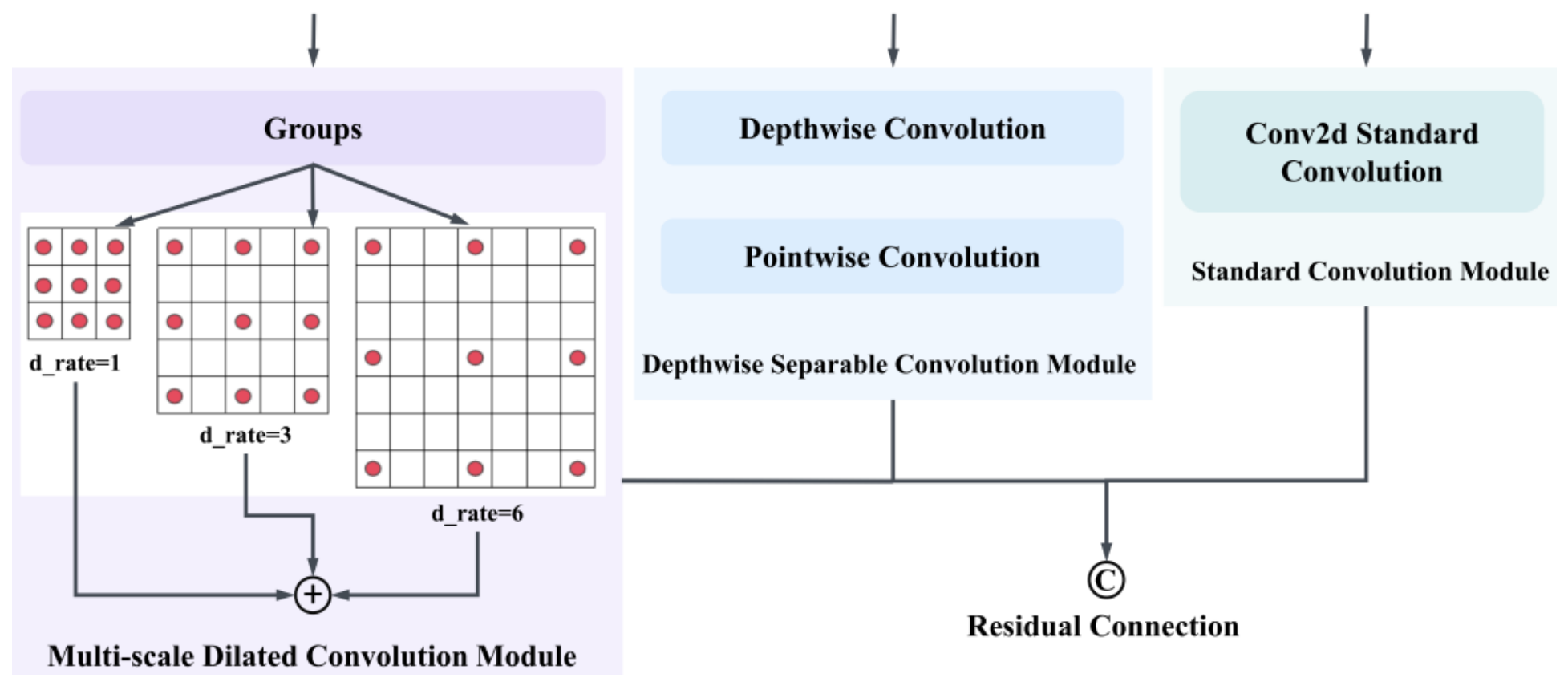
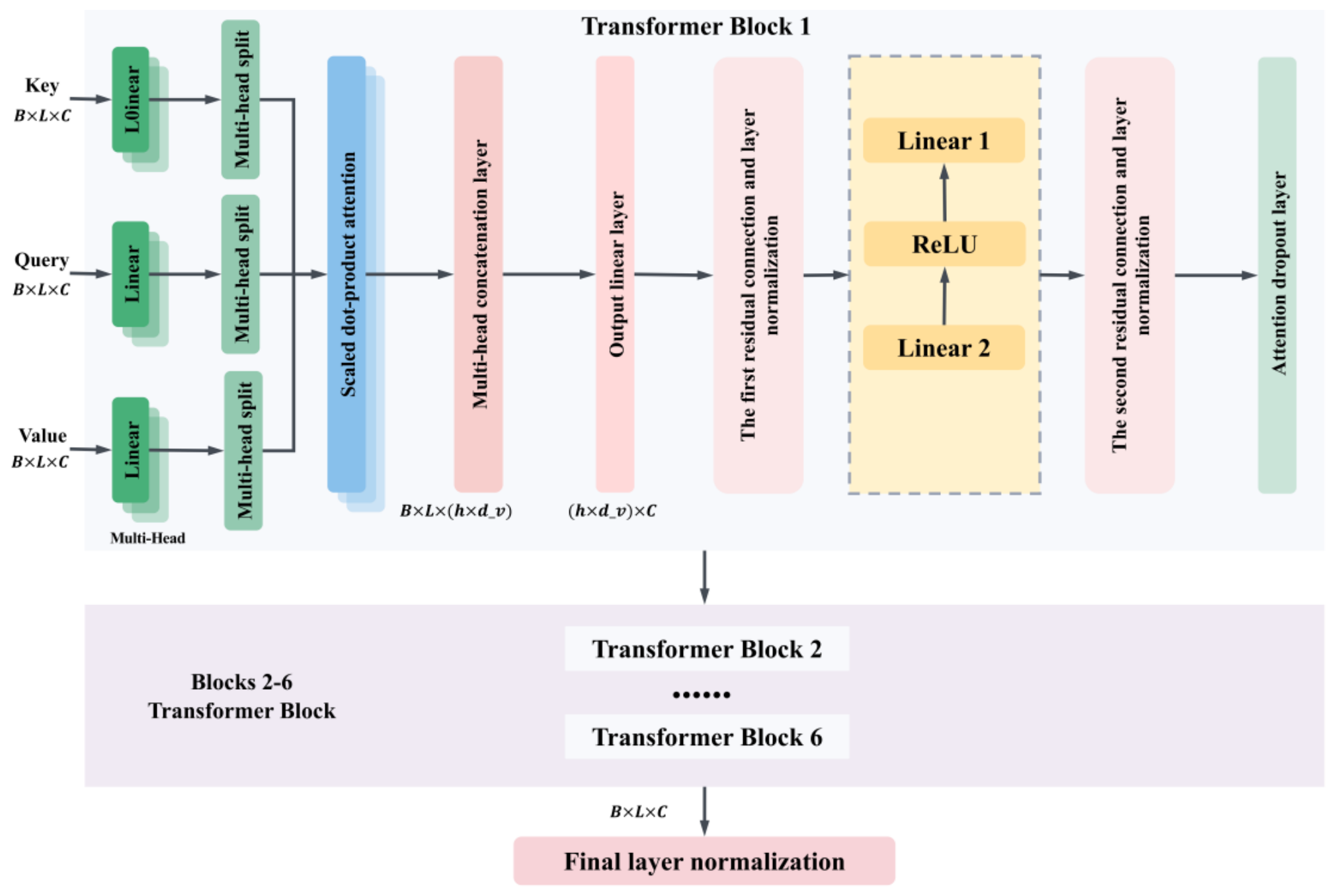
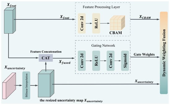
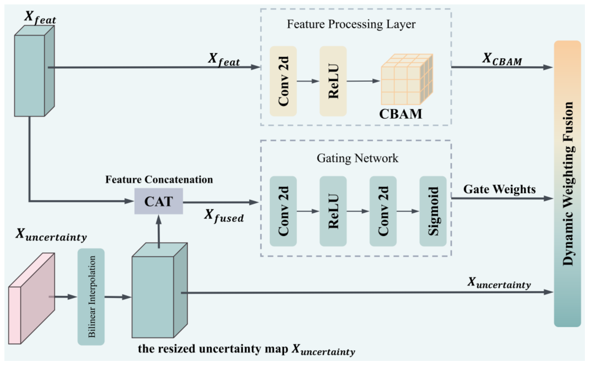
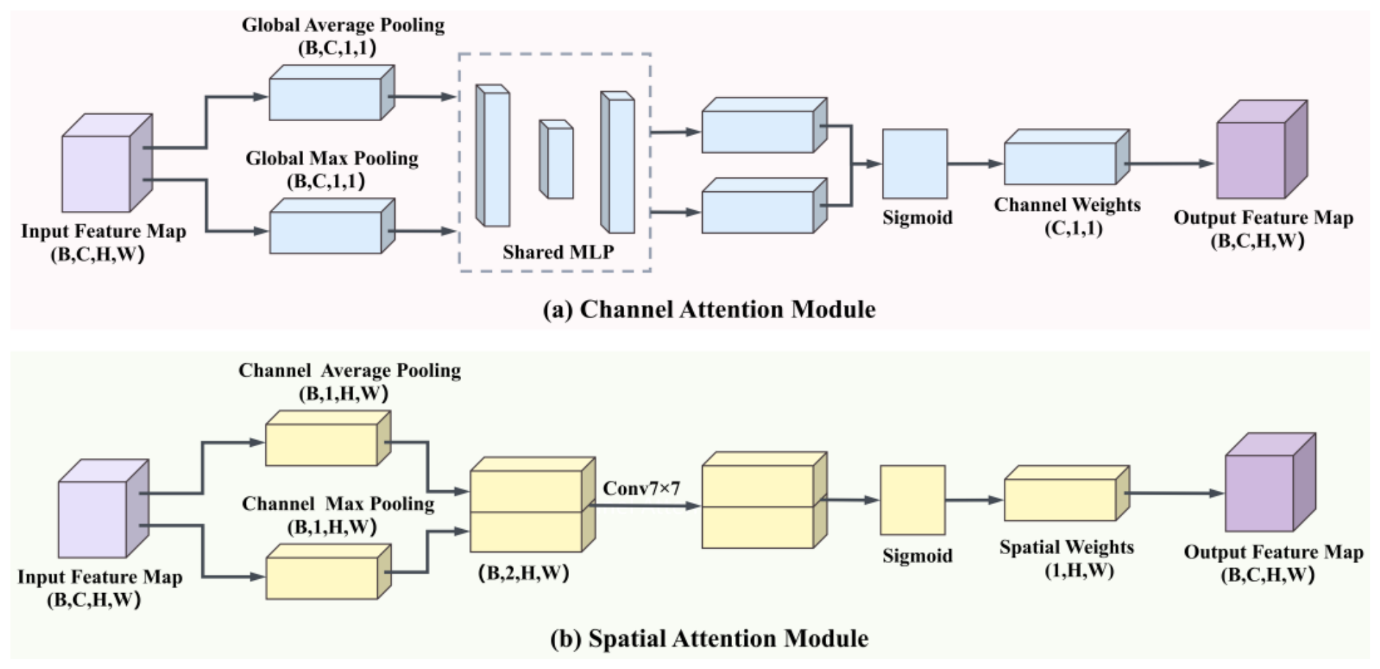
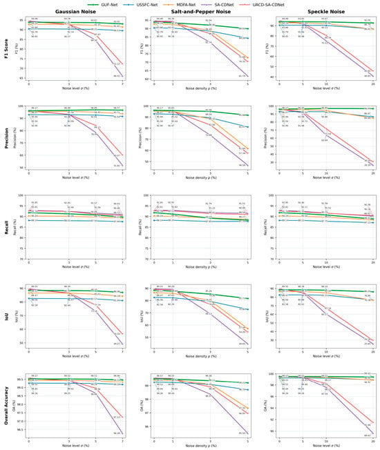
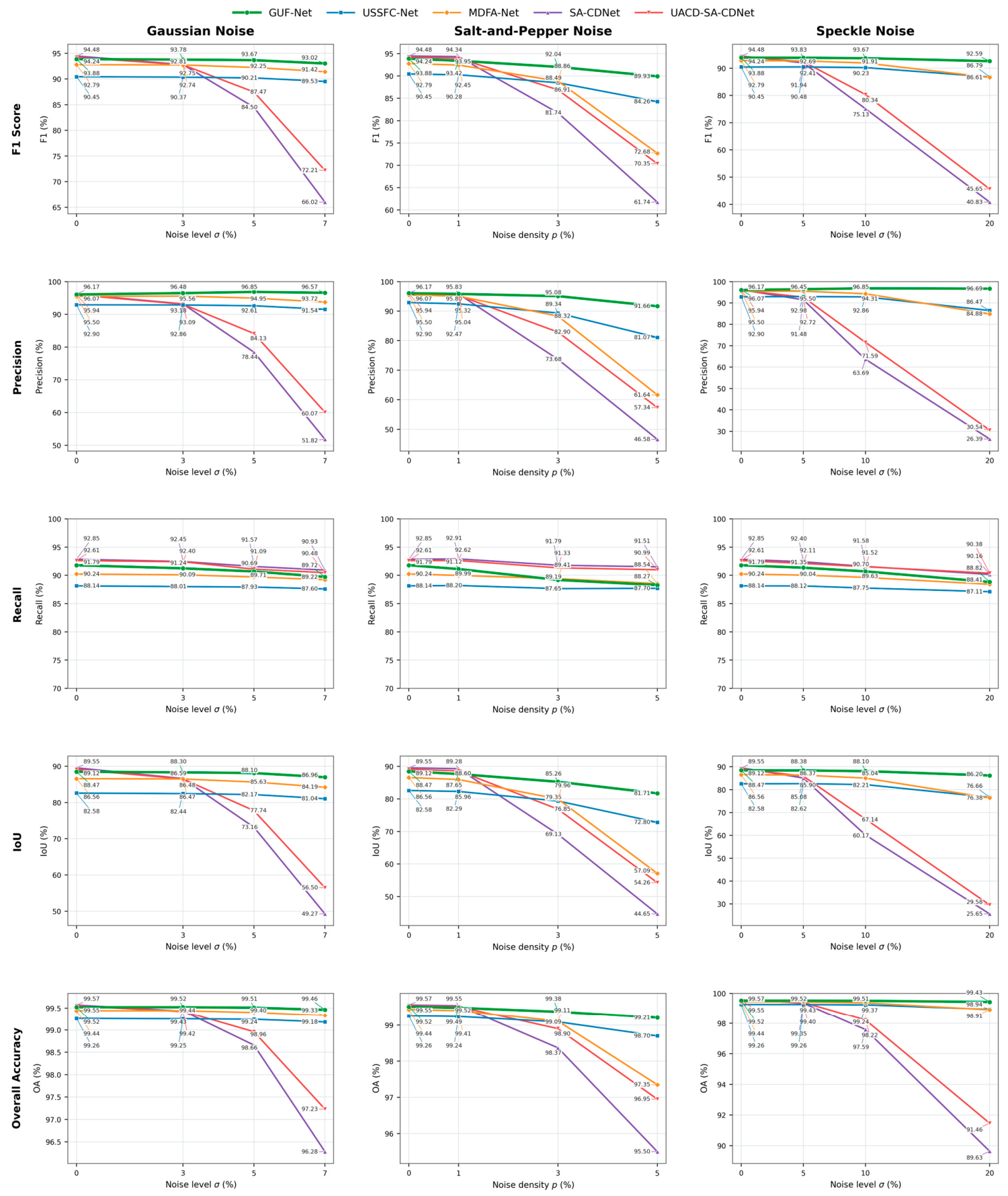
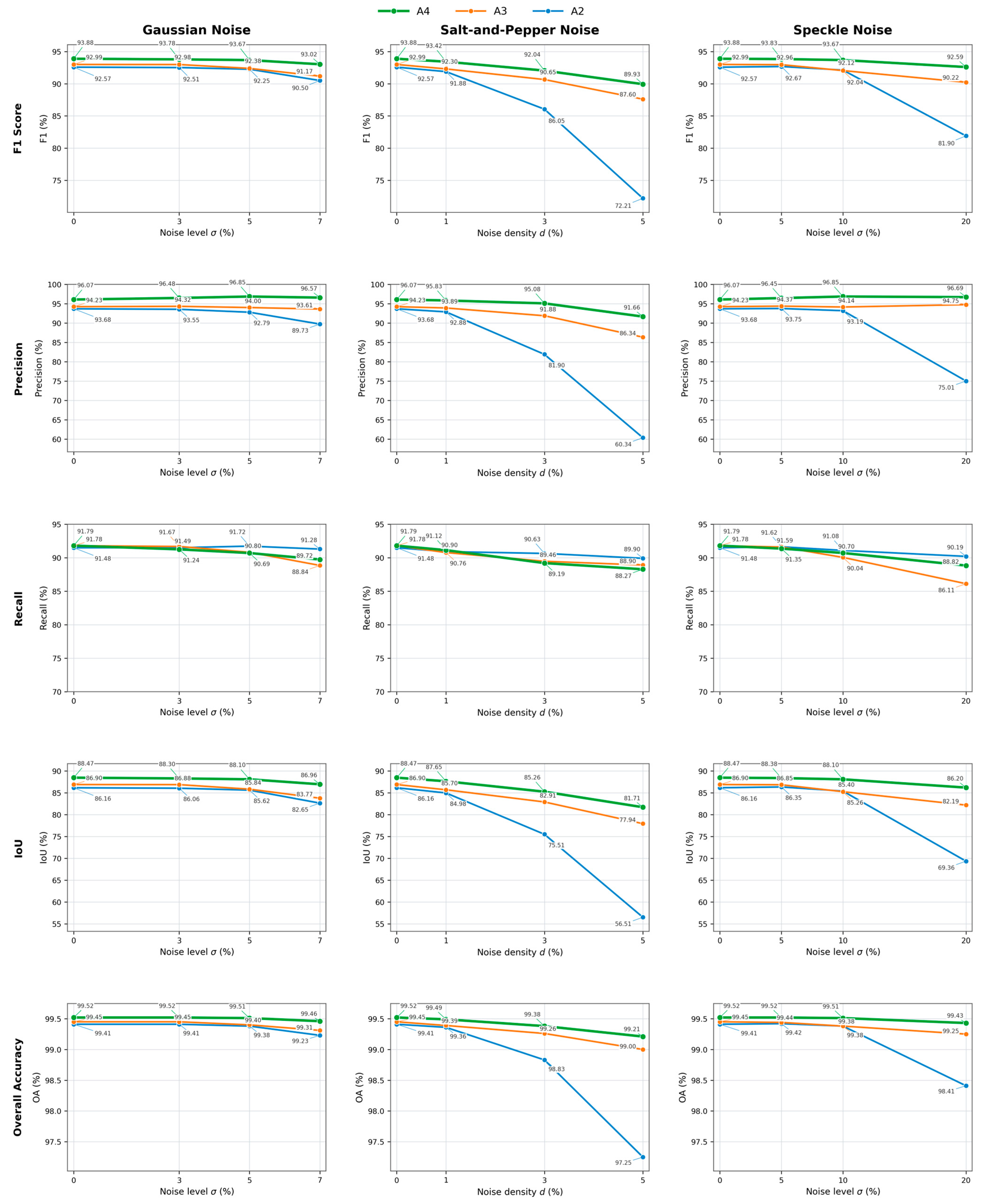
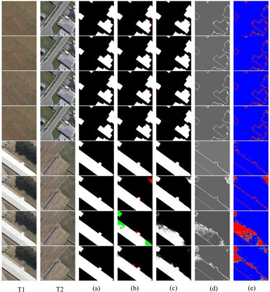
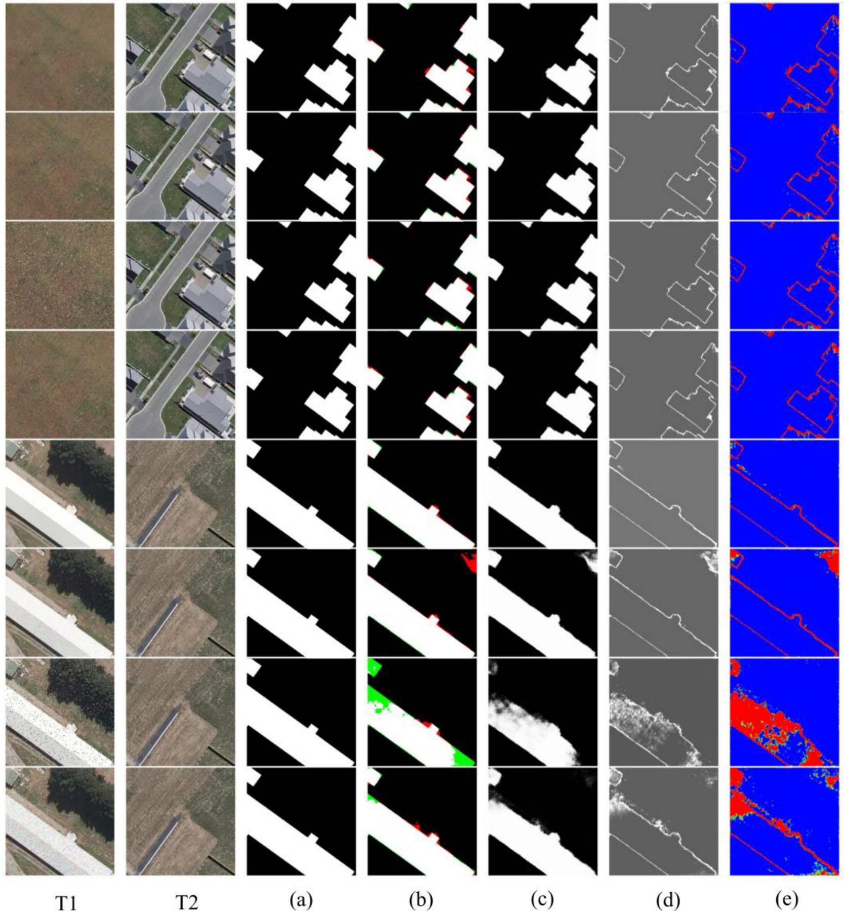
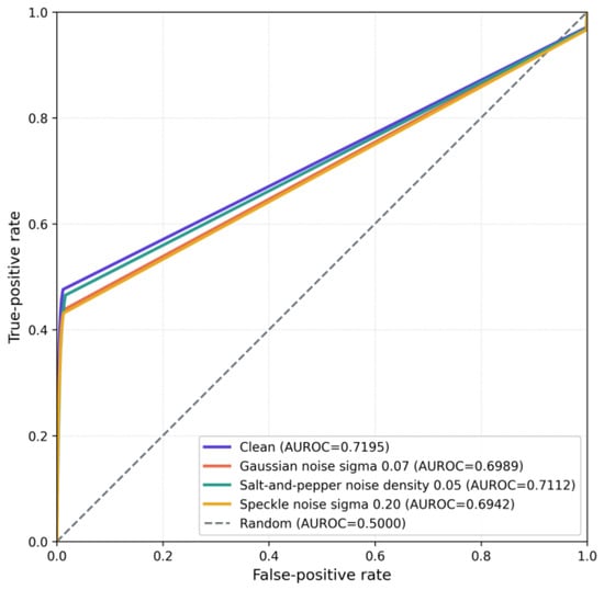
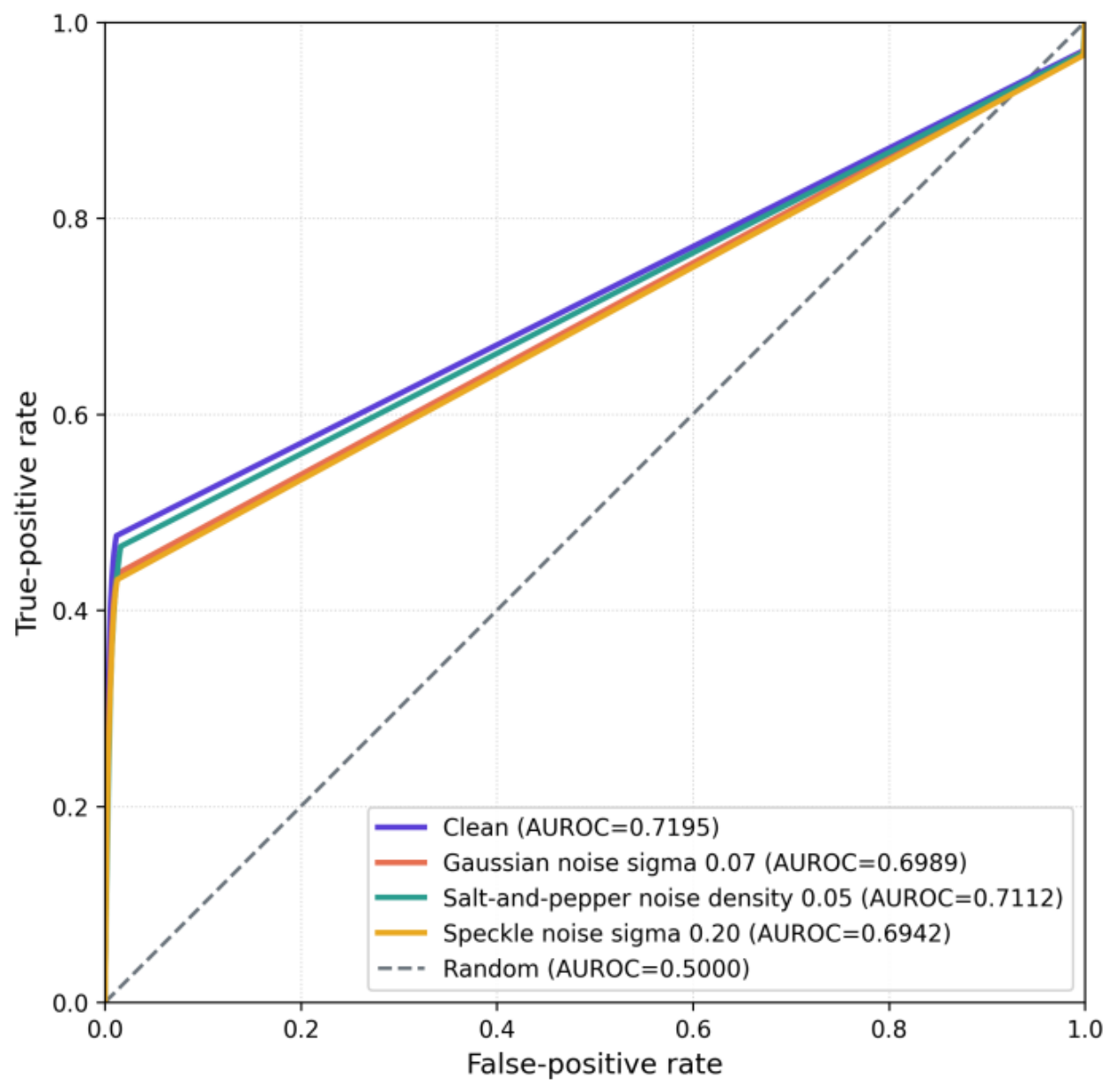

Disclaimer/Publisher’s Note: The statements, opinions and data contained in all publications are solely those of the individual author(s) and contributor(s) and not of MDPI and/or the editor(s). MDPI and/or the editor(s) disclaim responsibility for any injury to people or property resulting from any ideas, methods, instructions or products referred to in the content. |
© 2026 by the authors. Licensee MDPI, Basel, Switzerland. This article is an open access article distributed under the terms and conditions of the Creative Commons Attribution (CC BY) license.