


Highlights
What are the main findings?
- The proposed ED-iSwinLSTM-ND model achieved accurate 24-h global TEC forecasts under both high and low solar activity, outperforming the benchmark deep-learning models and the CODE C1PG product.
- The improved periodic shifted-window mechanism effectively mitigated the ±180° longitude boundary effect, reducing boundary prediction errors under both high and low solar activity.
What are the implications of the main findings?
- Incorporating the longitudinal periodic continuity and diurnal characteristics of global TEC improves the accuracy and stability of multi-step TEC forecasting.
- ED-iSwinLSTM-ND provides an effective deep-learning approach for short-term global ionospheric TEC forecasting under different solar activity levels.
Abstract
Accurate forecasting of global ionospheric total electron content (TEC) is important for space weather research and Global Navigation Satellite System (GNSS) applications. To address the complex spatiotemporal variability of TEC and the artificial discontinuity across the ±180° longitude boundary in global TEC maps, this study proposes an improved SwinLSTM model (iSwinLSTM) and further develops the ED-iSwinLSTM-ND framework for global TEC forecasting. By redesigning the shifted-window mechanism to account for longitudinal periodicity, iSwinLSTM enhances cross-boundary information interaction, while an Encoder–Decoder architecture combined with the Next-Day (ND) strategy enables prediction of the next 12 TEC maps from the preceding 36 maps. The model was evaluated retrospectively using archived GIMs from the selected test years. In 2025, a high solar activity year, the model achieved an MAE of 3.51 TECU, an RMSE of 5.10 TECU, and an R2 of 0.94; in 2020, a low solar activity year, the corresponding values were 0.96 TECU, 1.50 TECU, and 0.95. Boundary experiments further confirmed that the periodic shifted-window mechanism effectively reduces longitude-boundary errors. Overall, ED-iSwinLSTM-ND provides an effective framework for short-term global TEC forecasting by jointly exploiting spatiotemporal dependencies, longitudinal periodicity, and diurnal characteristics.
1. Introduction
The ionosphere is a partially ionized region of the upper atmosphere that affects transionospheric radio-wave propagation [1,2]. At GNSS frequencies, ionospheric propagation introduces a group delay in code observations and a phase advance in carrier-phase observations. To first order, these effects are proportional to the total electron content (TEC) along the signal path and inversely proportional to the square of the signal frequency [1,2]. Accurate ionospheric modeling is important for GNSS positioning, as demonstrated by improvements in positioning accuracy and convergence achieved using precise ionospheric corrections [3]. Consequently, characterizing and forecasting the spatiotemporal variability of TEC is important for ionospheric monitoring, space-weather assessment, and GNSS-related applications [4]. Total electron content (TEC) is a key parameter for characterizing ionospheric variability. Therefore, investigating its spatiotemporal evolution and developing high-accuracy forecasting models are of great significance for improving navigation and positioning accuracy.
However, owing to the complex spatiotemporal characteristics of the ionosphere and the combined influences of solar activity, geomagnetic disturbances, and variations in the middle and upper atmosphere, developing high-accuracy forecasting models remains a challenging task. Existing ionospheric forecasting methods can generally be classified into three categories: physics-based models, empirical models, and statistical models. Physics-based models are founded on ionospheric plasma transport and thermochemical processes and simulate physical processes such as photoionization, ion chemical reactions, diffusion and drift, neutral winds, electric fields, and particle precipitation by numerically solving the continuity, momentum, and energy equations for ions and electrons. Schunk et al. developed a time-dependent three-dimensional ionospheric model for middle and high latitudes that could simultaneously calculate the densities of multiple ion species as well as electron and ion temperatures [5]. Fuller-Rowell et al. developed a coupled thermosphere–ionosphere model that further described the dynamical and chemical coupling processes between the neutral atmosphere and the ionosphere [6]. Such models have strong physical interpretability and can provide a relatively comprehensive description of ionospheric evolution under different external forcing conditions. However, because they require the solution of multiple sets of coupled nonlinear equations and depend on numerous inputs, including solar radiation, geomagnetic activity, lower-atmospheric forcing, and boundary conditions, they are computationally expensive. Their forecasting results are also susceptible to uncertainties in external forcing parameters, which limits their application to real-time forecasting at high spatial and temporal resolutions [7]. In contrast, commonly used empirical ionospheric models include the International Reference Ionosphere (IRI) [8,9,10], NeQuick [11,12], and Bent models [13]. These models can characterize the mean variations and statistical distributions of TEC to a certain extent, but their ability to respond to anomalous disturbances, intense solar activity, and sudden space weather events is relatively limited, resulting in reduced forecasting performance under complex conditions. In addition to physics-based and empirical models, statistical models have been widely used for TEC forecasting, including the autoregressive moving average (ARMA) model, autoregressive integrated moving average (ARIMA) model, and linear time-series models. These methods establish forecasting relationships primarily based on the autocorrelation, trends, and periodicity of historical TEC sequences. Ratnam et al. proposed a TEC forecasting model combining linear time-series analysis with multivariate ARMA and incorporated factors such as solar extreme ultraviolet radiation, geomagnetic activity, periodic oscillations, and long-term trends as model inputs to characterize low-latitude ionospheric TEC variations [14]. Mandrikova et al. combined wavelet transform with the ARIMA model, using wavelet analysis to separate variations in ionospheric parameters at different temporal scales and subsequently applied ARIMA for forecasting and anomaly detection. The method was validated using TEC and ionospheric critical-frequency data [15]. Ansari et al. developed an improved linear time-series model using observations from 10 GNSS stations in southwestern Japan from 2011 to 2018 and incorporated solar and geomagnetic activity parameters to forecast and analyze the spatiotemporal variations in TEC [16]. Overall, conventional statistical models have relatively simple structures and high computational efficiency and can effectively capture linear trends, periodic characteristics, and short-term correlations in TEC sequences. However, these approaches generally rely on assumptions of stationarity or linear relationships, and most are designed for time-series modeling at individual stations or within limited regions. Consequently, they have difficulty fully characterizing the nonlinear behavior of TEC and the dynamic relationships among different spatial locations. When solar activity intensifies significantly or sudden events such as geomagnetic storms occur, historical statistical relationships may change, leading to degraded forecasting performance. Therefore, simultaneously learning the nonlinear variations and complex spatiotemporal dependencies of TEC remains an important challenge in improving ionospheric forecasting accuracy.
With the development of deep learning, neural networks, owing to their strong nonlinear mapping and feature extraction capabilities, provide a new approach to overcoming the linear assumptions of conventional statistical models and capturing the complex spatiotemporal evolution of TEC. Akhoondzadeh used a multilayer perceptron (MLP) to model TEC time series for the identification of pre-earthquake ionospheric anomalies, demonstrating that neural networks can effectively extract nonlinear variation characteristics from complex TEC sequences [17]. However, conventional recurrent neural networks are susceptible to vanishing or exploding gradients when processing long time sequences, making it difficult to effectively learn long-term dependencies. To address this problem, Hochreiter and Schmidhuber proposed the Long Short-Term Memory (LSTM) network, which introduces memory cells, input gates, forget gates, and output gates into the recurrent structure to selectively retain or update historical information, thereby enhancing the ability of the model to learn long-term temporal dependencies [18]. Sun et al. applied LSTM to vertical TEC forecasting over Beijing and demonstrated its effectiveness in TEC time-series forecasting [19]. Xiong et al. proposed an Encoder–Decoder Long Short-Term Memory (ED-LSTM) model, which encoded historical TEC sequences and progressively decoded future states, thereby improving multi-step TEC forecasting over China and outperforming conventional LSTM, ARIMA, and IRI-2016 methods [20]. In recent years, the Transformer architecture has demonstrated strong capabilities for modeling long-range dependencies through its self-attention mechanism, providing a new approach to spatiotemporal ionospheric TEC forecasting. However, the standard Transformer computes attention relationships between arbitrary pairs of positions, resulting in computational complexity that increases quadratically with the number of image-grid elements and imposing substantial computational and memory costs for high-resolution TEC map forecasting. To address this limitation, Liu et al. proposed the Swin Transformer, which restricts self-attention computation to non-overlapping local windows, allowing computational complexity to increase approximately linearly with image size. Meanwhile, shifted windows between adjacent network layers establish cross-window connections, while hierarchical feature representations enable multiscale spatial feature extraction [21]. The shifted-window mechanism allows windows in subsequent layers to cross the boundaries of those in preceding layers, thereby facilitating information interaction among different local regions while maintaining manageable computational costs. Although the Swin Transformer is effective in learning long-range dependencies, when used alone, it lacks memory states similar to those in LSTM, leaving room for improvement in the recurrent updating of historical information during continuous multi-step forecasting. To combine the advantages of self-attention and recurrent memory structures, Tang et al. proposed SwinLSTM, which integrates Swin Transformer modules with a simplified LSTM structure and replaces the convolutional state transitions in Convolutional Long Short-Term Memory (ConvLSTM) with self-attention operations. SwinLSTM learns long-term temporal dependencies through hidden and cell states while extracting spatial correlations using Swin Transformer modules, and it achieved better forecasting performance than ConvLSTM on several spatiotemporal forecasting datasets, including Moving MNIST, Human3.6M, TaxiBJ, and KTH [22]. However, the original SwinLSTM was primarily designed for general two-dimensional images and video sequences, and direct application to global TEC map forecasting requires consideration of the specific spatial characteristics of ionospheric data. On the one hand, global TEC exhibits periodic continuity in the longitudinal direction. On the other hand, conventional shifted windows with a fixed shifting direction primarily enhance local information exchange between adjacent windows but remain insufficient for modeling spatial dependencies between distant TEC regions. Moreover, the spatial scales and variation amplitudes of TEC change substantially with different solar activity levels. Therefore, the forecasting model must account for both the relatively stable variations during a low solar activity year and the stronger spatial gradients and day-to-day variability during a high solar activity year.
To address the aforementioned issues, this study proposes an improved SwinLSTM model based on an Encoder–Decoder architecture, termed ED-iSwinLSTM-ND. The model takes continuous TEC map sequences as input. Its encoder progressively extracts TEC distribution features at different spatial scales, while the decoder integrates and reconstructs multilevel spatiotemporal information. Meanwhile, a Next-Day (ND) forecasting strategy is introduced to establish correspondence between historical TEC sequences and the forecasting targets of the following day, enabling the model to more effectively learn cross-day temporal dependencies and day-to-day evolution patterns of TEC. Within the iSwinLSTM unit, multidirectional window shifts and corresponding attention masks are employed to enhance feature interactions among adjacent windows in different directions and improve information propagation across window boundaries as well as between the two longitudinal edges of the global TEC maps. Consequently, the proposed model can simultaneously characterize the multiscale spatial distributions, cross-regional dependencies, and cross-day evolution patterns of TEC, thereby improving the accuracy, stability, and boundary continuity of global TEC forecasting under different solar activity levels.
2. Dataset and Data Preprocessing
The ionospheric total electron content (TEC) data used in this study were obtained from the final global ionospheric map (GIM) products generated by the Center for Orbit Determination in Europe (CODE) and accessed through NASA’s Crustal Dynamics Data Information System (CDDIS). GIM data are typically provided in the IONosphere Map EXchange (IONEX) format and provide vertical total electron content (VTEC) values on a regular global latitude–longitude grid. In this study, the TEC data from GIM were used as a representation of the global ionospheric state to construct a spatiotemporal sequence dataset for global TEC forecasting.
The original GIM data cover the entire globe, ranging from 180°W to 180°E in longitude and from 87.5°S to 87.5°N in latitude. The data have a spatial resolution of 5° in longitude and 2.5° in latitude and a temporal resolution of 2 h, corresponding to 12 global TEC maps per day. To evaluate the forecasting capability of the model under different solar activity levels, global TEC data from the low solar activity years of 2019–2020 and the high solar activity years of 2024–2025 were selected for the experiments. The low solar activity years were used to evaluate the forecasting performance of the model under relatively stable ionospheric conditions, whereas the high solar activity years were used to assess its generalization capability under conditions characterized by enhanced TEC variability and more complex spatial structures.
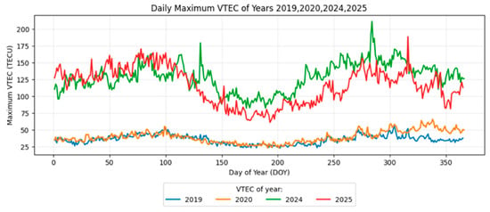
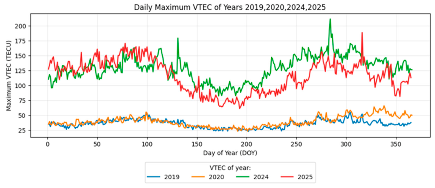
Figure 1 illustrates the differences among the datasets used in this study. Each curve represents the VTEC values for the same calendar date in a given year. As shown in Figure 1, the VTEC values in 2019 and 2020 were generally low, ranging from approximately 25 to 70 TECU. In 2024 and 2025, the VTEC values increased substantially to approximately 75–175 TECU, while the highest overall values were observed in 2024, reaching up to 211 TECU.
Figure 1.
The low solar activity years (2019 and 2020) were characterized by relatively moderate solar activity, whereas the high solar activity years (2024 and 2025) exhibited pronounced VTEC variations.
To ensure consistent input dimensions, the original TEC data were first processed to obtain a uniform spatial grid. The original TEC maps typically have a grid size of 71 × 73. To accommodate the window partitioning and shifted-window operations in the proposed model, the TEC maps were uniformly transformed into a regular 72 × 72 grid. After preprocessing, the TEC map at each time step can be represented as: where () denotes the global TEC map at time step (t), and the last dimension represents the single-channel TEC feature.
Considering the substantial differences in TEC value ranges across different years and different solar activity levels, min–max normalization was further applied to map the TEC data to a consistent numerical range, thereby improving the stability of model training. The normalized data were used for model training, and after forecasting, the predicted values were transformed back to the original TEC units through inverse normalization for error calculation and result analysis.
For sample construction, the global TEC forecasting problem is formulated as a sequence-to-sequence spatiotemporal regression task. Based on consecutive TEC map sequences, a sliding temporal window is employed to construct the input samples and prediction targets. As shown in Figure 2, four consecutive days of TEC maps are used to construct each sample, with 36 TEC maps from the first three days serving as the input and 12 TEC maps from the fourth day serving as the output. For a sample whose input sequence ends at time step t, the input sequence and the corresponding prediction target are defined as follows:
where denotes a single global TEC map at time step t, while and denote the historical input sequence and the future prediction target sequence, respectively.
Figure 2.
Generation of the TEC dataset using a sliding window.
For regression tasks, a loss function is employed during neural network training to evaluate the discrepancy between the predicted and reference values. The optimization algorithm uses the gradient of the loss function to minimize the residual errors over all samples in the training set. During each training epoch, the residual errors are first estimated, the gradients of the loss function are then computed, and the weights and biases of the neural network are subsequently updated by the optimizer. This training cycle is repeated for a predefined number of epochs or until an early-stopping criterion is satisfied.
3. Method
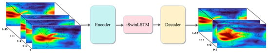
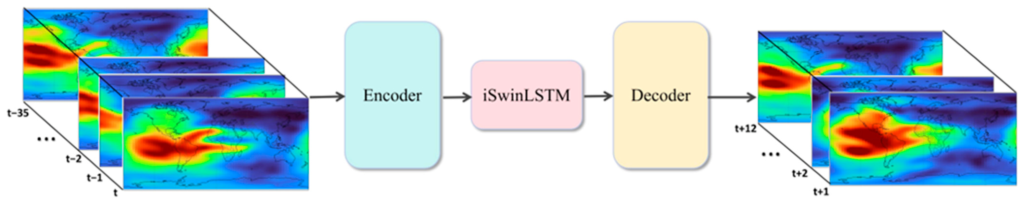
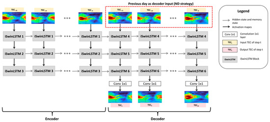
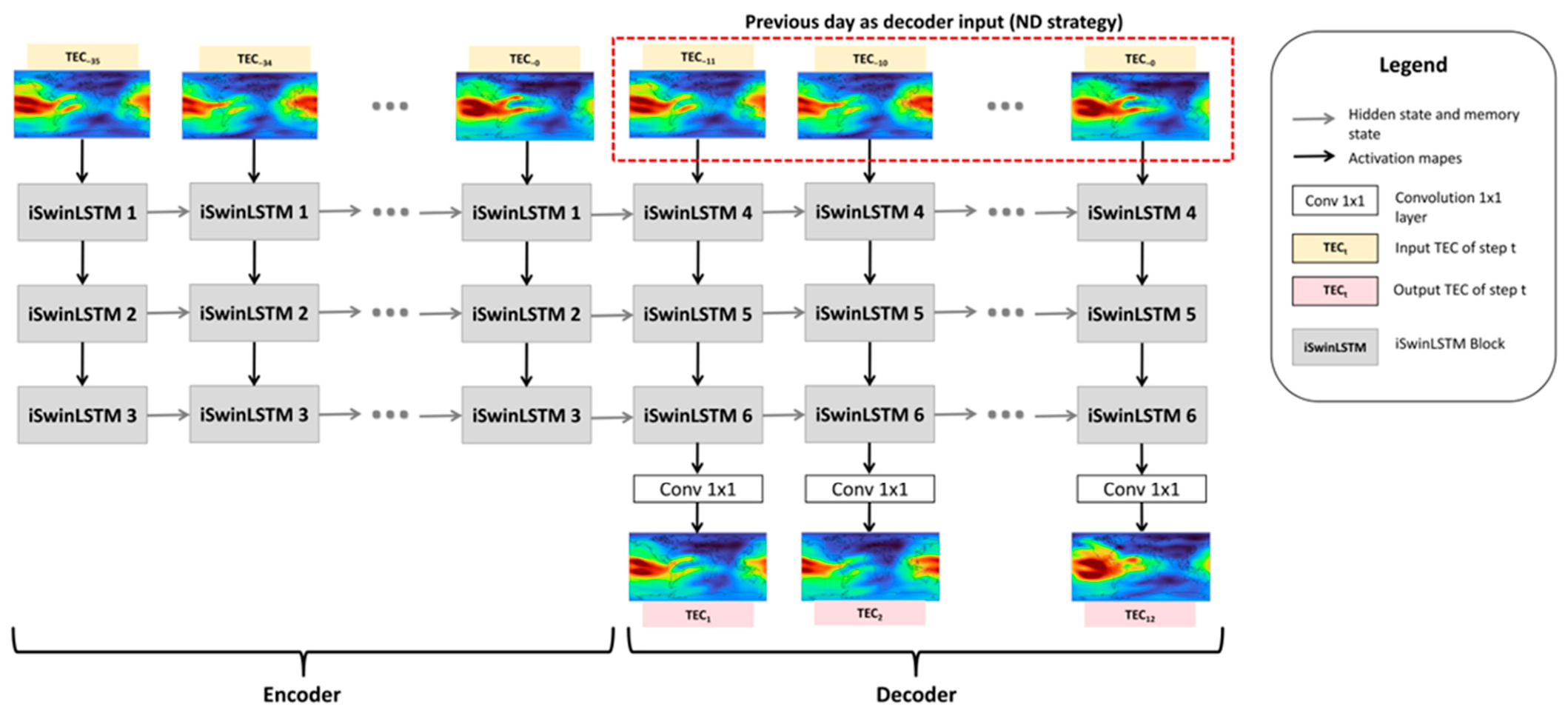
iSwinLSTM is a variant of SwinLSTM that incorporates a longitudinal extension scheme into the shifted-window attention mechanism. To address the discontinuity at the longitude boundary caused by the planar representation of global TEC maps, the shifted-window mechanism in SwinLSTM is improved to better capture the spatial continuity and periodic boundary characteristics of global TEC maps. On this basis, the ED-iSwinLSTM-ND forecasting model is further developed. The model employs an Encoder–Decoder architecture to extract spatiotemporal features from historical TEC sequences and incorporates the actual TEC maps from the previous day as inputs to the decoder, enabling multi-step forecasting of future global TEC maps. The overall framework is illustrated in Figure 3.
Figure 3.
Basic architecture of the proposed ED-iSwinLSTM-ND model.
3.1. iSwinLSTM
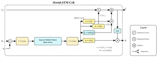
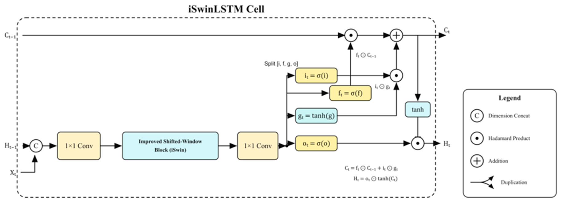
During map projection, the spherical surface of the Earth is typically represented as a two-dimensional rectangular plane at a certain scale. Owing to the projection, the +180° and −180° longitudes, which are adjacent on the actual spherical surface, are separated and located at the left and right edges of the planar map, respectively, resulting in an artificial spatial discontinuity. For global TEC maps, the spatial distribution of TEC exhibits a certain degree of continuity and periodicity in the longitudinal directions because the ionosphere is jointly influenced by multiple factors, including solar activity, geomagnetic disturbances, and variations in the middle and upper atmosphere. However, the planar representation of global TEC maps weakens the spatial correlation between regions on the two sides of the longitude boundary, making the forecasting model susceptible to boundary effects and consequently affecting the spatial continuity and fine-scale representation of global TEC forecasts. To address this issue, an iSwinLSTM unit was designed in this study, as illustrated in Figure 4.
Figure 4.
Schematic diagram of the iSwinLSTM cell.
iSwinLSTM jointly models spatiotemporal sequence data by integrating the window-based self-attention mechanism of the Swin Transformer into the LSTM architecture. Specifically, iSwinLSTM employs self-attention within local windows to dynamically capture correlations among different spatial locations, thereby enabling a more flexible representation of spatial dependencies in global TEC maps. At time step t, the basic state-update process of iSwinLSTM can be expressed as:
where denotes the input TEC feature map at the current time step; and denote the hidden state and cell state at the previous time step, respectively; and and denote the updated hidden state and cell state at the current time step, respectively.
For window-based self-attention computation, the input features are first partitioned into a set of non-overlapping windows. Let the input features within a given window be denoted by . The Query (Q), Key (K), and Value (V) are obtained through linear projections as follows:
where , and denote the projection matrices for the Query, Key, and Value, respectively. The self-attention within each window is computed as follows:
where d denotes the dimension of each attention head, B denotes the relative position bias, and M denotes the mask matrix. Through this mechanism, the model dynamically captures the correlations among different grid points within each window according to the current spatial distribution of TEC and performs weighted aggregation of spatial contextual information.
However, the shifting mechanism in the original SwinLSTM is primarily designed for general two-dimensional images. The left and right boundaries of ordinary images are typically not connected in the actual spatial domain. Therefore, after cyclic shifting, an attention mask is required to prevent information interaction between spatially unrelated regions. In contrast, global TEC maps are two-dimensional representations of the spherical ionosphere, in which the +180° and −180° longitudes are geographically adjacent and exhibit distinct longitudinal periodic continuity. If the original masking strategy is directly applied, the inherently continuous TEC structures at the left and right edges of the global map are artificially separated, which may reduce the forecasting accuracy in the boundary regions.
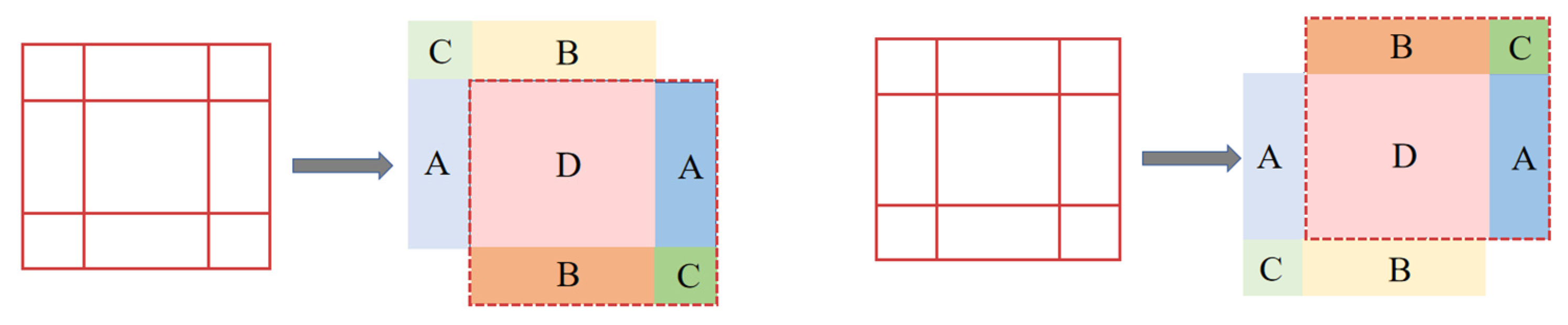
To address this issue, an iSwinLSTM unit was designed in this study. To alleviate the spatial discontinuity along the longitudinal direction in global TEC maps, a longitudinal extension strategy was incorporated into the shifted-window attention mechanism. For the standardized 72 × 72 global TEC grid, the window partitioning scheme was reorganized through periodic shifting, thereby enhancing the model’s ability to capture spatial dependencies across the longitude boundary. Two complementary periodic shifting operations were employed in this study. The first operation performs a shift toward the lower-right direction:
The second operation performs a shift toward the upper-right direction:
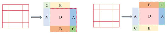
where denotes the cyclic shifting operation, and and represent the feature maps after the lower-right and upper-right shifts, respectively. The TEC maps used in this study had a spatial size of 72 × 72, and the shift size was set to one-quarter of the map dimension, corresponding to 18 grid cells, as illustrated in Figure 5. Through the complementary lower-right and upper-right shifts, the model captures cross-boundary spatial information from different window configurations, thereby enhancing its ability to represent longitudinally periodic and continuous spatial structures.
Figure 5.
Schematic diagram of the improved shifted-window block. Blue, orange/yellow, green, and pink denote regions A, B, C, and D, respectively. The red dashed box outlines the region after shifting. The extended region A is included in the attention computation, whereas regions B and C are masked.
During the shifted-window attention computation, a selective attention mask M is further introduced to prevent erroneous information interaction between spatially unrelated regions. The improved window-based self-attention is computed as follows:
where = 0 indicates that the attention weights between positions i and j can be computed normally, whereas = indicates that the attention interaction between the two positions is masked. By incorporating the mask matrix into the attention scores, the range of information interaction among different regions can be controlled. Considering the longitudinal periodic boundary characteristics of global TEC maps, cross-boundary connections are preserved in the longitudinal direction, allowing regions at the left and right edges of the map to participate in the same attention computation. Meanwhile, shifted regions that should not be directly adjacent in the latitudinal direction are selectively masked to avoid introducing physically unreasonable spatial relationships.
Within the iSwinLSTM unit, the current input and the hidden state from the previous time step are first concatenated along the channel dimension:
The concatenated features are then projected through a 1 × 1 convolution:
The mapped features are then fed into the improved Swin Window Block to model spatial dependencies:
where the Swin Window Block incorporates the improved shifted-window and selective masking mechanisms. Subsequently, the gating components of the LSTM are generated through a 1 × 1 convolution:
is split along the channel dimension into four gating components, , , , and , corresponding to the pre-activation features of the input gate, forget gate, candidate memory, and output gate, respectively. Subsequently, the corresponding activation functions are applied to obtain the gate states:
where denotes the Sigmoid activation function, denotes the hyperbolic tangent function, and denotes element-wise multiplication. In this way, iSwinLSTM preserves the temporal memory capability of LSTM while incorporating an improved window-based attention mechanism specifically designed to account for the longitudinal periodic boundary of global TEC maps, thereby enhancing the model’s ability to capture the spatial continuity of TEC and the characteristics of boundary regions.
3.2. ED-iSwinLSTM-ND
Building upon the iSwinLSTM unit, the ED-iSwinLSTM-ND model is further developed in this study for multi-step global TEC forecasting, as illustrated in Figure 6. The model adopts an Encoder–Decoder architecture, in which the encoder extracts spatiotemporal evolution features from historical TEC sequences, while the decoder generates TEC forecasts for multiple future time steps conditioned on the encoded states. Compared with direct recursive forecasting, the Encoder–Decoder architecture separates historical feature extraction from future sequence generation, making it more suitable for sequence-to-sequence multi-step forecasting of global TEC.
Figure 6.
Architecture of ED-iSwinLSTM-ND. The input sequence from TEC-35 to TEC-0 is sequentially processed to generate the hidden and cell states, which are subsequently passed to the decoder. The decoder takes the GIMs from the previous day as inputs and generates the predicted GIMs for the following day.
Let the sequence of consecutive TEC maps be defined as:
where denotes the global TEC map at time step t. A sliding-window approach is employed to construct the input sequences and prediction targets. Let and denote the lengths of the input and prediction windows, respectively. The model input is then defined as:
The corresponding prediction target is defined as:
The model aims to learn the following mapping:
where denotes the ED-iSwinLSTM-ND model, denotes the learnable parameters of the model, denotes the historical TEC input sequence, denotes the decoder input sequence under the ND strategy, and denotes the predicted future TEC sequence.
The encoder consists of multiple stacked iSwinLSTM units. For the -th encoder layer, its input at time step k is denoted by . When , the input is the TEC map at the corresponding time step; when , the input is the hidden state of the preceding layer at the current time step. Accordingly, the layer-wise inputs and state update process can be expressed as follows:
After processing the input sequence, the encoder obtains the final hidden and cell states of each layer:
where L denotes the number of encoder layers. This set of states contains the spatial distribution information and temporal evolution information extracted from the historical TEC sequence and is used to initialize the decoder.
To fully exploit the diurnal variation characteristics of TEC, the Next-Day (ND) strategy is introduced into the decoder. The ND strategy refers to a next-day forecasting mechanism. Since TEC is strongly influenced by solar radiation, Earth’s rotation, and variations in local time, the spatial distributions of TEC at the same time on two consecutive days generally exhibit a certain degree of similarity. Therefore, using the observed TEC map at the corresponding time on the previous day as the decoder input provides an effective diurnal reference for forecasting TEC on the following day.
Given a prediction window length of , the decoder input sequence is defined as follows:
For the m-th prediction step, the decoder input is defined as:
Each decoder layer is initialized with the final hidden and cell states of the corresponding encoder layer:
For the -th decoder layer, its input at the m-th prediction step is denoted by . The first decoder layer takes the ND input as its current input, whereas each higher layer receives the hidden state of the preceding layer at the current prediction step. Accordingly, the state update process of each decoder layer can be expressed as follows:
Finally, the hidden state of the last decoder layer is mapped to a single-channel TEC prediction map through a 1 × 1 convolution:
Therefore, the overall forecasting process of ED-iSwinLSTM-ND can be expressed as follows:
The proposed model offers two main advantages. First, the encoder can extract spatiotemporal evolution patterns of the ionosphere from a relatively long historical TEC sequence, including diurnal variation characteristics, short-term disturbance features, and spatial distribution patterns. Second, the ND decoding strategy uses the observed TEC maps from the previous day as decoder inputs. Consequently, the model does not rely solely on hidden states to directly generate future TEC maps; instead, it learns the evolution of TEC for the following day based on the observed spatial distribution from the previous day. This strategy helps reduce error accumulation during multi-step forecasting and improves the stability of the prediction results.
In summary, iSwinLSTM primarily addresses the modeling of spatial dependencies and longitudinal boundary continuity in global TEC maps, whereas ED-iSwinLSTM-ND provides an overall framework for multi-step mapping from historical TEC sequences to future TEC sequences. By integrating these two components, the model can simultaneously exploit the spatial continuity, longitudinal periodicity, and temporal diurnal characteristics of global TEC, thereby improving the accuracy and stability of multi-step global ionospheric TEC forecasting.
4. Results
As described in Section 2, TEC maps from 2019 (a low solar activity year) and 2024 (a high solar activity year) were used as training samples, while TEC maps from 2020 (a low solar activity year) and 2025 (a high solar activity year) were used as test samples. The forecasting performance of different models was compared under high and low solar activity conditions. In this study, one widely used time-series forecasting model (LSTM), six spatiotemporal forecasting models (ConvLSTM, SwinLSTM, iSwinLSTM, ED-ConvLSTM-ND, ED-SwinLSTM-ND, and ED-iSwinLSTM-ND), and C1PG were compared. C1PG is a one-day-ahead TEC prediction product provided by the Center for Orbit Determination in Europe (CODE). It has been reported that C1PG achieves higher prediction accuracy for global TEC maps than the products provided by two other Ionosphere Associate Analysis Centers (IAACs), namely the European Space Agency (ESA) and Universitat Politècnica de Catalunya (UPC) [23].
Since the LSTM model can only predict TEC at individual grid points and cannot directly generate TEC maps, separate LSTM models were trained and used for prediction at each grid point in the study area. The resulting predictions were then reconstructed into TEC maps for comparison with the experimental results.
The proposed ED-iSwinLSTM-ND model was implemented using TensorFlow/Keras. The input and output tensors had shapes of B × 36 × 72 × 72 × 1 and B × 12 × 72 × 72 × 1, respectively, where B denotes the batch size and the remaining dimensions represent time, latitude, longitude, and the TEC channel. At a temporal resolution of 2 h, the model used the preceding three days of TEC maps to forecast the following day. Under the ND strategy, the last 12 maps of the historical input sequence were supplied to the decoder, without using reference maps from the forecast target period as inputs. Model parameters were optimized using Adam, with learning rates of 10−4 for the experiments. The batch size was set to 2, and training was limited to a maximum of 200 epochs. The mean absolute error (MAE) between the predicted and reference TEC maps in the normalized domain was used as the loss function. Validation loss was monitored during training, and early stopping with restoration of the best monitored weights was employed to limit overfitting. Predictions were subsequently transformed back to TECU using the normalization parameters saved for the corresponding training year. Forecasting performance was evaluated using MAE, root mean square error (RMSE), and the coefficient of determination (R2).
4.1. Evaluation Metrics
To quantitatively evaluate the forecasting performance of ED-iSwinLSTM-ND, the root mean square error (RMSE), mean absolute error (MAE), and coefficient of determination (R2) were calculated as follows:
where n denotes the total number of pixels in the predicted layer, denotes the VTEC value at the i-th pixel of the predicted layer obtained from the dataset through the sliding-window sampling process, denotes the VTEC value estimated by the model, and denotes the mean value of .
4.2. Experiments
4.2.1. Boundary Forecasting Performance of iSwinLSTM
Table 1 compares the forecasting performance of SwinLSTM and iSwinLSTM in the left and right longitudinal boundary regions and over the global domain for the high solar activity year (2025) and the low solar activity year (2020). The boundary metrics assess forecasting accuracy near the longitudinal edges targeted by the improved shifted-window mechanism, while the global metrics determine whether these local improvements are accompanied by an overall accuracy gain. iSwinLSTM achieved lower MAE and RMSE than SwinLSTM in all three evaluation regions in both years, indicating that the boundary improvements are accompanied by lower global forecasting errors.
Table 1.
Boundary and global forecasting performance of SwinLSTM and iSwinLSTM under different solar activity levels.
In 2025, iSwinLSTM reduced the left-boundary MAE from 5.37 to 4.55 TECU and RMSE from 7.54 to 6.34 TECU, corresponding to reductions of 15.27% and 15.92%, respectively. At the right boundary, MAE decreased from 4.88 to 4.54 TECU and RMSE from 6.61 to 6.34 TECU, with reductions of 6.97% and 4.08%. Over the global domain, MAE decreased from 4.24 to 4.11 TECU and RMSE from 5.98 to 5.68 TECU, representing reductions of 3.07% and 5.02%. The substantially larger reductions at the left boundary than over the global domain indicate a particularly pronounced improvement in this boundary region. Meanwhile, the reduction in global errors shows that the boundary improvement is accompanied by a net gain in overall forecasting accuracy.
A further feature of the 2025 results is the reduced difference in forecasting errors between the two boundaries. For SwinLSTM, the left-boundary MAE and RMSE exceeded their right-boundary counterparts by 0.49 and 0.93 TECU, respectively. For iSwinLSTM, these differences decreased to 0.01 TECU for MAE and zero for RMSE at the reported precision. This indicates more balanced forecasting accuracy between the two longitudinal edges. As described in Section 3.1, the modified shifting and masking operations allow information exchange across the longitudinal boundary while retaining restrictions on inappropriate latitudinal connections. The reduced boundary errors and smaller left–right error differences are consistent with the intended role of this design.
In 2020, iSwinLSTM also improved forecasting accuracy in both boundary regions. At the left boundary, MAE decreased from 1.36 to 1.25 TECU and RMSE from 1.93 to 1.80 TECU, corresponding to reductions of 8.09% and 6.74%, respectively. At the right boundary, the corresponding values decreased from 1.21 to 1.14 TECU and from 1.67 to 1.59 TECU, with reductions of 5.79% and 4.79%. Globally, MAE decreased from 1.26 to 1.22 TECU and RMSE from 1.95 to 1.79 TECU, representing reductions of 3.17% and 8.21%. Thus, the relative MAE reductions at both boundaries exceeded the global reduction, whereas the global RMSE reduction exceeded that at either boundary. This difference shows that the improvement depends on both the evaluation region and the metric, and is not uniformly concentrated at the map edges. Because RMSE gives greater weight to larger errors, its larger relative reduction than MAE over the global domain is consistent with a reduction in the influence of larger prediction deviations.
Taken together, the two experiments show that iSwinLSTM improves both boundary and global forecasting accuracy relative to SwinLSTM. The global MAE reductions were similar in 2025 and 2020, at 3.07% and 3.17%, respectively, while the global RMSE reduction was greater in 2020. In contrast, the strongest boundary improvement occurred at the left boundary in 2025. The benefit of the proposed modifications therefore varies across regions, metrics, and solar activity conditions. Overall, these results support the effectiveness of incorporating longitudinal periodicity into the shifted-window mechanism, with improvements in boundary forecasting accompanied by lower global errors in both test years.
4.2.2. Comprehensive Forecasting Performance of ED-iSwinLSTM-ND
Following the evaluation of the boundary and global forecasting performance of iSwinLSTM, the complete ED-iSwinLSTM-ND framework was compared with C1PG and the baseline deep-learning models under different solar activity conditions. As shown in Table 2, ED-iSwinLSTM-ND achieved the lowest MAE and RMSE in both test years. In 2025, its MAE and RMSE were 3.51 and 5.10 TECU, respectively, with an R2 of 0.94. In 2020, the corresponding values were 0.96 TECU, 1.50 TECU, and 0.95. These results demonstrate an overall accuracy advantage across the two test years.
Table 2.
Forecasting performance under different solar activity levels.
LSTM exhibited the largest forecasting errors in both years, with MAE and RMSE values of 10.42 and 13.89 TECU in 2025 and 3.21 and 4.79 TECU in 2020. Its R2 values were also substantially lower, at 0.58 and 0.49, respectively. This performance should be interpreted in relation to the pointwise implementation used in this study: a separate LSTM model was trained for each grid point, and the resulting predictions were subsequently assembled into global TEC maps. Consequently, each model learns the temporal evolution of an individual location without directly accessing the spatial context provided by surrounding or more distant regions. Although local temporal histories contain useful predictive information, this implementation cannot explicitly exploit the spatial relationships represented in TEC maps.
The models employing the ED–ND framework consistently achieved lower MAE and RMSE than their corresponding standalone models. This pattern highlights the benefit of combining historical sequence encoding with a structured reference for future sequence generation. In particular, the ND strategy supplies the decoder with the observed TEC map at the corresponding time on the previous day for each prediction step. As described in Section 3.2, this design exploits the day-to-day similarity associated with the diurnal behavior of TEC, providing an explicit spatial reference from which the decoder can learn the changes required for the following day. The decoder therefore receives a time-aligned reference throughout the forecast horizon, rather than relying exclusively on the encoded states. In the present experiments, these reference maps were taken from the historical portion of each archived sequence and remained fixed throughout the 24-h prediction window. Consequently, the decoder does not use its previously predicted TEC maps as subsequent inputs, avoiding the direct propagation of prediction errors through map feedback. Errors may nevertheless arise when the target-day TEC evolution departs from the previous-day reference in ways that the model cannot adequately infer from the historical sequence.
For ED-iSwinLSTM-ND, the improvements relative to standalone iSwinLSTM were 14.60% in MAE and 10.21% in RMSE in 2025, increasing to 21.31% and 16.20%, respectively, in 2020. The larger relative gains in 2020 were consistent with the usefulness of a previous-day reference when day-to-day TEC evolution is more regular. Within the same ED–ND framework, ED-iSwinLSTM-ND further reduced MAE and RMSE relative to ED-SwinLSTM-ND by 2.50% and 2.49% in 2025 and by 1.03% and 0.66% in 2020. Relative to ED-ConvLSTM-ND, the corresponding reductions were 8.36% and 6.93% in 2025 and 4.95% and 0.66% in 2020. Thus, the improved recurrent unit provides additional gains within the complete framework.
The CODE one-day predicted global ionospheric map product, C1PG, provides an additional benchmark for prediction accuracy over the selected test periods [24]. In 2025, ED-iSwinLSTM-ND reduced MAE from 3.85 to 3.51 TECU and RMSE from 5.50 to 5.10 TECU, corresponding to reductions of 8.83% and 7.27%, respectively, while R2 increased from 0.93 to 0.94. In 2020, MAE decreased from 1.04 to 0.96 TECU and RMSE from 1.53 to 1.50 TECU, representing reductions of 7.69% and 1.96%, respectively, while R2 remained at 0.95. The proposed model therefore improved both error metrics in both years, but its RMSE advantage over C1PG was considerably smaller in 2020. This indicates that the low-solar-activity advantage is more evident in average absolute error than in the metric that gives greater weight to larger deviations.
Overall, the results are consistent with the rationale of combining spatial–temporal modeling with an explicit previous-day reference. The pointwise LSTM results highlight the limitations of forecasting each location independently, while the improvements obtained with the ED–ND models support the use of historical sequence encoding together with time-aligned decoder inputs. ED-iSwinLSTM-ND combines these features with the improved spatial modeling examined in Section 4.2.1 and achieved the lowest aggregate errors in both test years. The results support the effectiveness of this combined design.
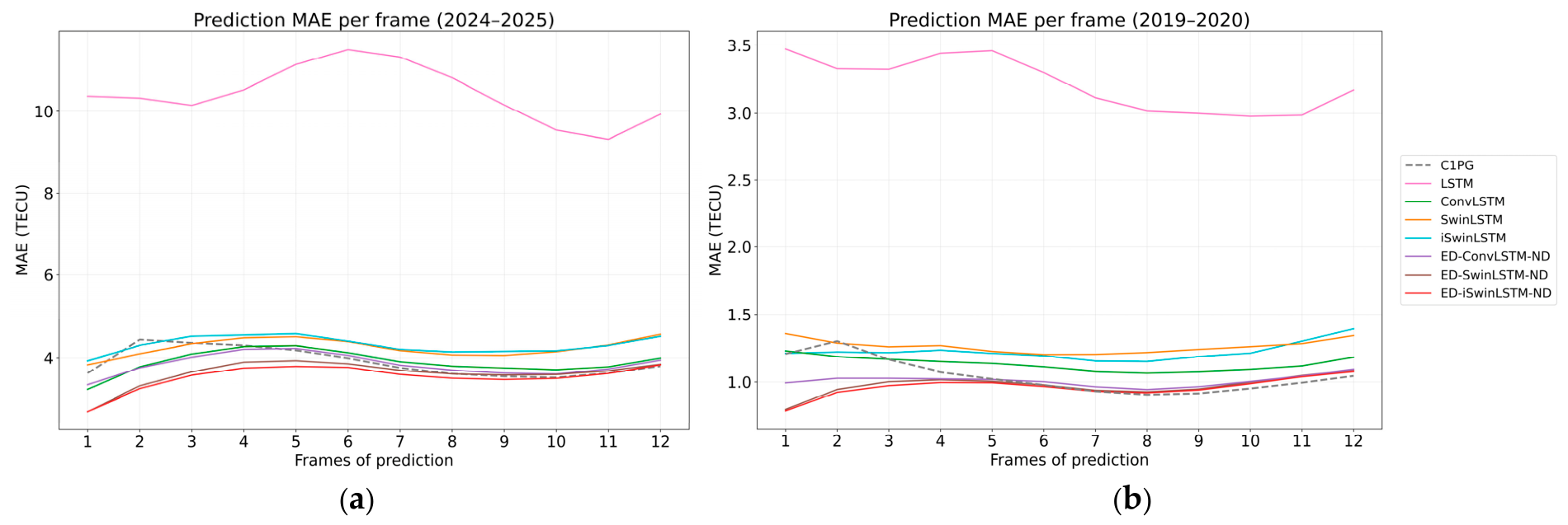
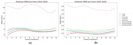
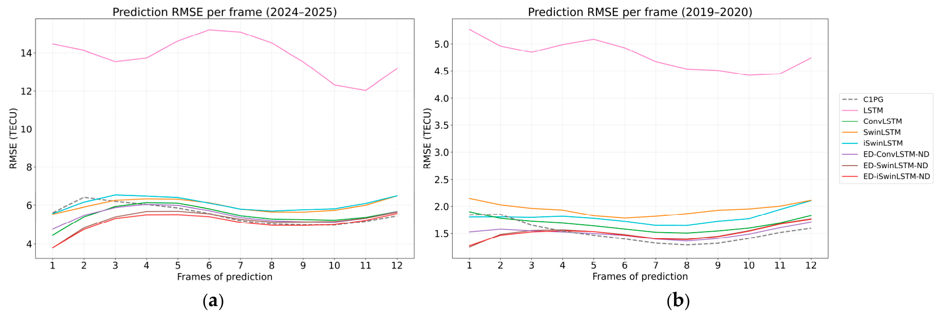
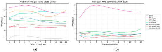
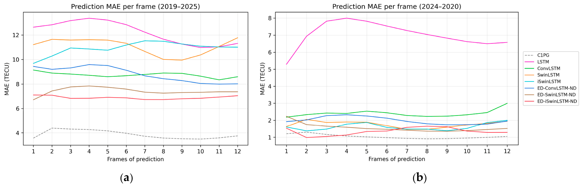
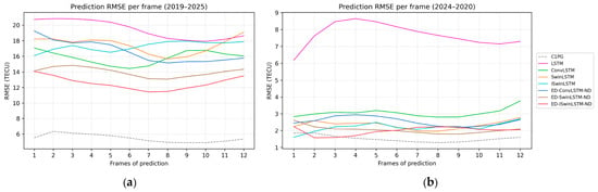
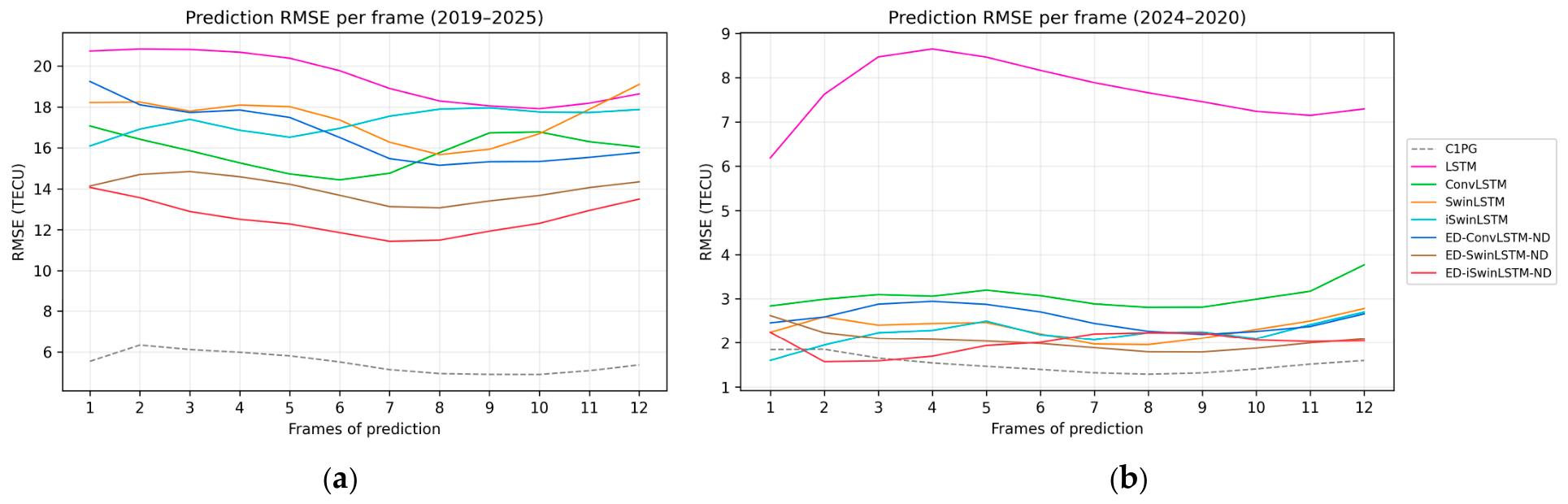
Under high solar activity conditions (2024–2025) and low solar activity conditions (2019–2020), the MAE (Figure 7) and RMSE (Figure 8) at the 12 future prediction steps were calculated for each model to compare their stepwise forecasting performance and error evolution characteristics at different forecast lead times.
Figure 7.
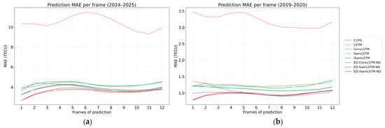
Stepwise MAE of different models under two training–testing year settings: (a) trained on 2024 and tested on 2025; (b) trained on 2019 and tested on 2020. The forecast lead times range from 2 to 24 h at 2 h intervals. The MAE at each lead time is calculated using all test samples and their corresponding 72 × 72 spatial grids.
Figure 8.
Stepwise RMSE of different models under two training–testing year settings: (a) trained on 2024 and tested on 2025; (b) trained on 2019 and tested on 2020. The forecast lead times range from 2 to 24 h at 2 h intervals. The RMSE at each lead time is calculated using all test samples and their corresponding 72 × 72 spatial grids.
As shown in Figure 7, clear differences can be observed in the frame-by-frame MAE among the different models. In the 2024–2025 experiment, the MAE of LSTM was substantially higher than that of the other models and exhibited relatively pronounced fluctuations across the prediction steps, indicating that relying solely on temporal sequence information is insufficient to adequately characterize the complex spatiotemporal variations of global TEC. Except for LSTM, the MAE values of the remaining models were generally concentrated within a relatively low range, although noticeable differences still existed among them. The errors of ConvLSTM and SwinLSTM were generally higher than those of the models employing an encoder–decoder architecture, whereas ED-ConvLSTM-ND, ED-SwinLSTM-ND, and ED-iSwinLSTM-ND exhibited relatively lower stepwise errors. Among them, ED-iSwinLSTM-ND maintained a comparatively low MAE across the 12 prediction steps and demonstrated better forecasting accuracy than the other models overall. Although ED-SwinLSTM-ND or C1PG showed comparable performance at some prediction steps, the error curve of ED-iSwinLSTM-ND generally remained at a lower level, indicating its strong multi-step forecasting capability under relatively high solar activity conditions.
In the 2019–2020 experiment, the MAE values of all models were generally substantially lower than those in 2024–2025, indicating that global TEC variations are relatively more stable during periods of weaker solar activity and that the corresponding forecasting task is less challenging. The MAE of LSTM remained clearly higher than that of the other models and stayed at a relatively high level throughout the entire prediction horizon. In contrast, the errors of ConvLSTM, SwinLSTM, and the models with encoder–decoder structures were markedly reduced, among which ED-ConvLSTM-ND, ED-SwinLSTM-ND, and ED-iSwinLSTM-ND exhibited relatively similar error curves. ED-iSwinLSTM-ND achieved the lowest or nearly the lowest MAE at most prediction steps and maintained an error level comparable to or even lower than that of C1PG. The MAE of ED-iSwinLSTM-ND varied non-monotonically with forecast lead time, with an initial increase, a subsequent decrease, and a renewed increase toward the end of the forecast horizon. Its errors nevertheless remained comparatively low across the evaluated lead times.
The frame-by-frame variation in RMSE shown in Figure 8 generally follows a pattern consistent with that of MAE. In the 2024–2025 experiment, the RMSE of LSTM was substantially higher than that of the other models and exhibited relatively large temporal fluctuations. ConvLSTM and SwinLSTM showed the next highest RMSE values, whereas the models employing encoder–decoder structures achieved further reductions in overall error. ED-iSwinLSTM-ND maintained the lowest or nearly the lowest RMSE at most prediction steps. In particular, during the middle and later prediction stages, its error curve remained relatively stable, demonstrating good forecasting stability.
In the 2019–2020 experiment, the RMSE values of all models were likewise clearly lower than those under high solar activity conditions. LSTM still exhibited the largest forecasting errors, while ConvLSTM and SwinLSTM showed relatively higher RMSE values than the encoder–decoder-based models. Among them, ED-iSwinLSTM-ND achieved a relatively low RMSE during the early prediction stages and maintained superior or nearly optimal performance at several subsequent prediction steps, indicating that it can preserve good forecasting accuracy under different solar activity levels.
Considering the frame-by-frame variations in both MAE and RMSE, model performance was influenced not only by forecast lead time but also closely related to solar activity levels. Compared with the low solar activity period, the forecasting errors of all models were generally substantially larger in 2024–2025, indicating that the spatiotemporal variations of TEC are more complex under stronger solar activity conditions and impose greater demands on the feature extraction and long-term forecasting capabilities of the models. The conventional LSTM model exhibited substantially larger errors than the other models in both experiments, suggesting that modeling temporal dependencies alone is insufficient to adequately characterize changes in the spatial structure of global TEC. After incorporating spatial feature extraction mechanisms, the forecasting performance of ConvLSTM and SwinLSTM was markedly improved, while the models employing encoder–decoder structures further reduced the stepwise forecasting errors. Overall, ED-iSwinLSTM-ND maintained relatively low MAE and RMSE values under both solar activity conditions and across different forecast lead times, while its error curves remained comparatively stable. These results indicate that the combination of the encoder–decoder architecture, the improved spatiotemporal feature extraction mechanism of iSwinLSTM, and the ND strategy contributes to improving the accuracy and stability of multi-step global TEC forecasting.
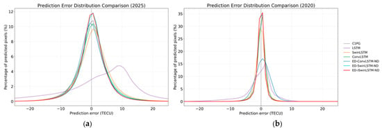
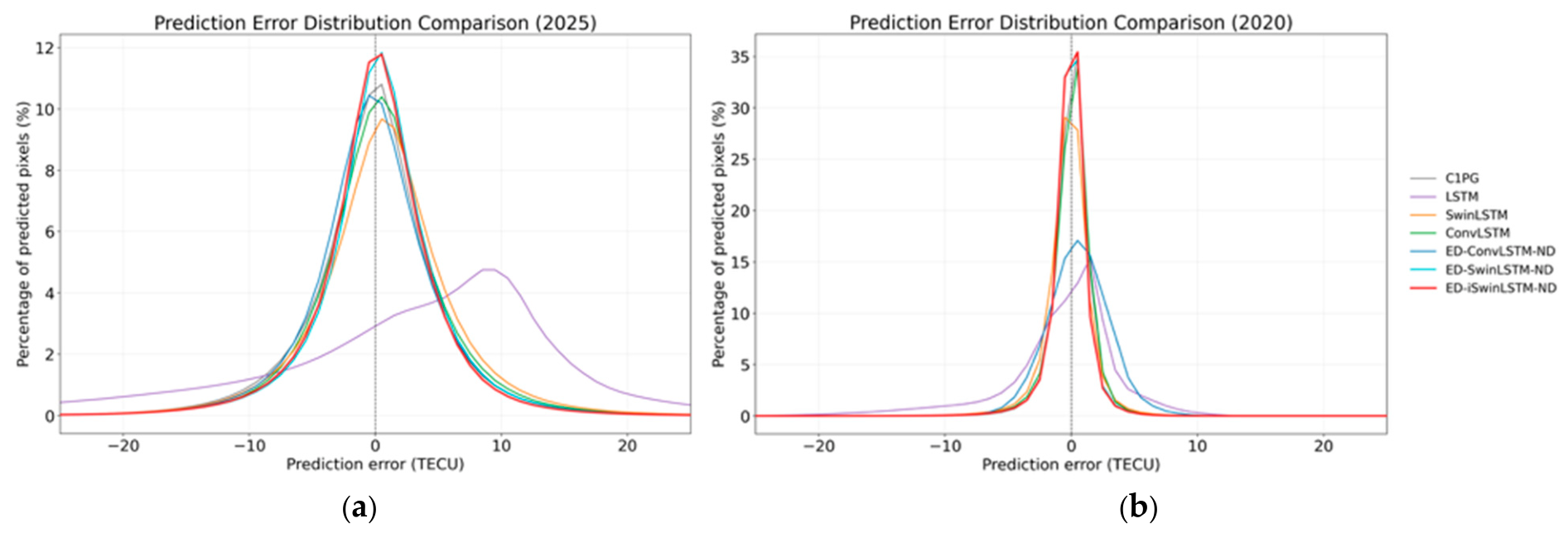
As shown in Figure 9a, the prediction errors of all models were generally concentrated around 0 TECU. Among them, LSTM exhibited a relatively broad error distribution, with its peak clearly deviating from 0 TECU, indicating comparatively large prediction errors. In contrast, the error distributions of ConvLSTM, SwinLSTM, and the ED-based models were more concentrated. The proposed ED-iSwinLSTM-ND exhibited a relatively high distribution peak near 0 TECU, with most errors confined to a narrow range, demonstrating better error concentration than ED-SwinLSTM-ND and ED-ConvLSTM-ND.
Figure 9.
TEC prediction error distributions of different models under two training–testing year settings: (a) trained on 2024 and tested on 2025; (b) trained on 2019 and tested on 2020. The prediction error is defined as the predicted value minus the observed value. The vertical axis represents the percentage of spatiotemporal grid points within each error interval relative to the total number of grid points included in the statistics, and the gray dashed line indicates zero error.
As shown in Figure 9b, the error distributions of all models became further concentrated around 0 TECU. Among them, ED-iSwinLSTM-ND exhibited the highest distribution peak and the peak closest to 0 TECU, together with a relatively narrow error distribution range. These results indicate that the proposed model can maintain small prediction biases and stable forecasting performance across different yearly datasets.
Deep-learning models learn complex spatiotemporal relationships in TEC evolution from historical data. Their forecasting capability depends not only on model architecture but may also be constrained by how well the training data represent the target forecasting conditions. Training data from a low-solar-activity year may not adequately capture the range of TEC amplitudes and spatiotemporal variations encountered under high solar activity. Consequently, forecasting performance achieved when training and testing under similar solar activity levels does not establish that the same accuracy can be maintained under different activity conditions. To examine this issue, this study evaluated transfer in both directions across solar activity levels: training on low-activity data from 2019 and testing on high-activity data from 2025, and training on high-activity data from 2024 and testing on low-activity data from 2020. These experiments assess model generalization when the solar activity conditions differ markedly between training and testing.
As shown in Table 3, all evaluated deep-learning models exhibited increases in both MAE and RMSE relative to the results in Table 2 for the same test years, where training and testing were conducted under similar solar activity levels. This indicates that forecasting across solar activity levels presents an additional challenge for these models. Nevertheless, ED-iSwinLSTM-ND achieved the lowest MAE and RMSE and the highest R2 in both settings. For 2019 → 2025, its MAE and RMSE were 6.89 and 12.59 TECU, respectively, representing reductions of 7.14% and 10.01% relative to the second-best model, ED-SwinLSTM-ND, while R2 increased from 0.57 to 0.65. For 2024 → 2020, its MAE and RMSE were 1.34 and 1.99 TECU, respectively, representing reductions of 13.55% and 2.93% relative to ED-SwinLSTM-ND, while R2 increased from 0.90 to 0.91.
Table 3.
Cross-year generalization performance of TEC forecasting models.
These results demonstrate that the proposed model maintains the best overall forecasting accuracy among the evaluated deep-learning models in both transfer directions. However, its performance still deteriorated relative to training and testing under similar solar activity levels, particularly when transferring from a low-activity year to a high-activity year. Insufficient representation of the target activity conditions in the training data may be one factor contributing to this deterioration, although this explanation requires further verification through broader temporal coverage and analysis of the training and test data distributions. Thus, although the proposed model retains a relative advantage in forecasting across solar activity levels, its adaptability to different activity conditions remains an area for improvement.
To further examine how cross-activity generalization varies with forecast lead time, Figure 10 presents the MAE for forecasts from 2 to 24 h under the two settings. For 2019 → 2025, ED-iSwinLSTM-ND maintained the lowest MAE among the evaluated deep-learning models throughout the forecast horizon, with relatively modest variation across lead times. Its aggregate advantage therefore reflects improvements across the horizon rather than gains at only a few lead times. ED-SwinLSTM-ND generally produced the next-lowest errors, whereas standalone SwinLSTM and iSwinLSTM did not outperform ConvLSTM, indicating clear differences in model performance under this transfer setting. For 2024 → 2020, all models except LSTM exhibited lower MAE overall, and the gaps between their curves narrowed. ED-iSwinLSTM-ND achieved the lowest or close to the lowest MAE at several lead times but was surpassed by other models at some intermediate lead times. Thus, its best aggregate result in Table 3 represents performance across the complete forecast horizon and does not imply superiority at every individual lead time.
Figure 10.
MAE at each forecast lead time for different models under two cross-year evaluation settings: (a) training on 2019 data and testing on 2025 data; (b) training on 2024 data and testing on 2020 data. Forecast lead times range from 2 to 24 h at 2 h intervals. MAE at each lead time is computed over all test samples and all grid cells on the 72 × 72 spatial grid.
The RMSE results in Figure 11 further characterize model performance with greater emphasis on larger prediction deviations. For 2019 → 2025, the RMSE of ED-iSwinLSTM-ND was close to that of ED-SwinLSTM-ND at the first lead time and remained lower thereafter. Its curve initially decreased, reached a relatively low level in the middle-to-late portion of the forecast horizon, and then increased again. This non-monotonic pattern indicates that the dependence of forecasting error on lead time cannot be described simply as continuous accumulation with successive prediction steps. For 2024 → 2020, the RMSE curves of ED-iSwinLSTM-ND and ED-SwinLSTM-ND were more closely grouped and crossed at some lead times, consistent with their small aggregate RMSE difference of 0.06 TECU in Table 3. It should also be noted that for 2019 → 2025, both the MAE and RMSE of the proposed model remained substantially higher than those of the C1PG reference product at every evaluated lead time. The lead-time results therefore support its overall advantage over the other evaluated deep-learning models while also revealing the remaining performance gap when transferring from low to high solar activity.
Figure 11.
RMSE at each forecast lead time for different models under two cross-year evaluation settings: (a) training on 2019 data and testing on 2025 data; (b) training on 2024 data and testing on 2020 data. Forecast lead times range from 2 to 24 h at 2 h intervals. RMSE at each lead time is computed over all test samples and all grid cells on the 72 × 72 spatial grid.
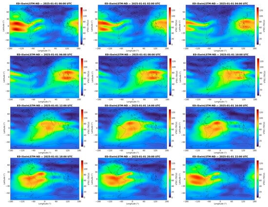
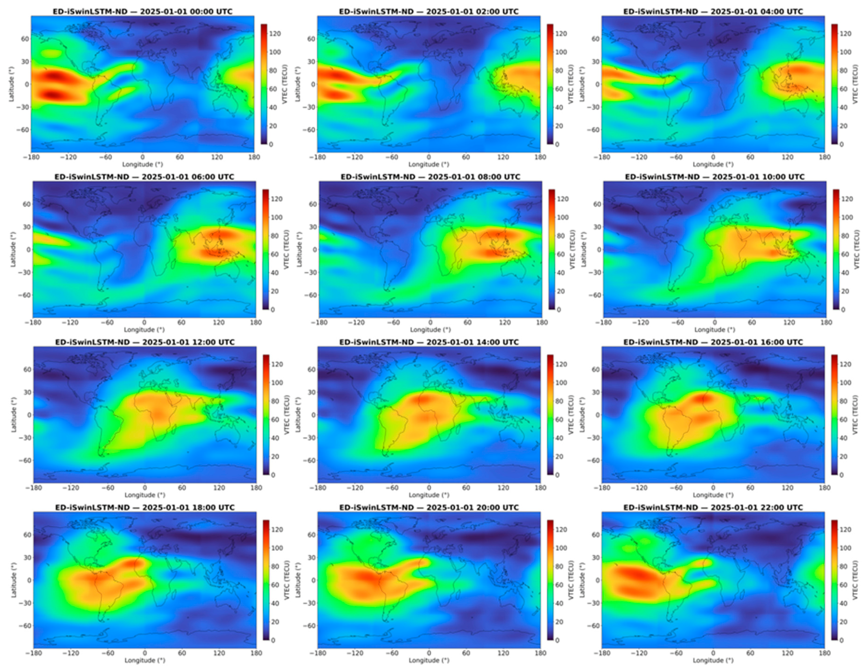
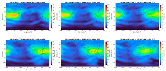
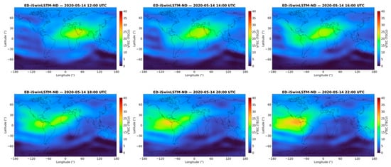
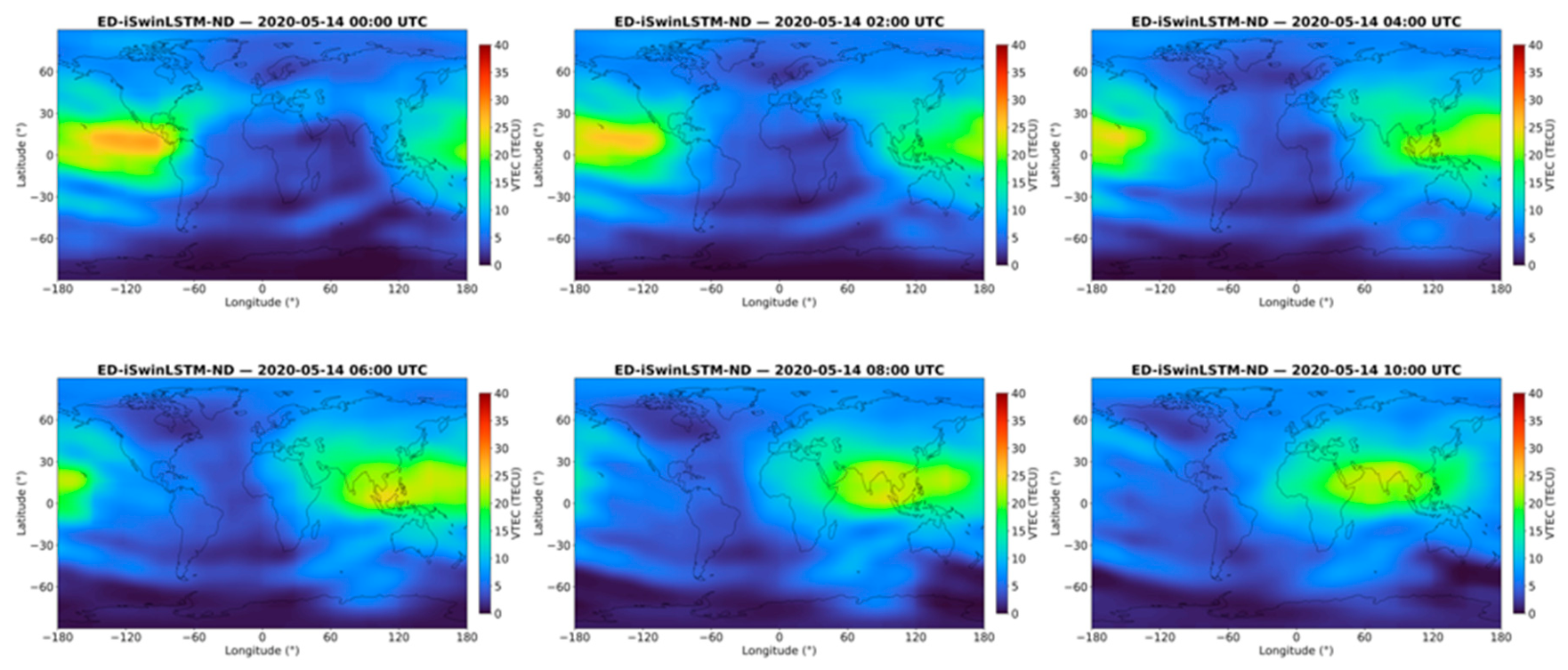
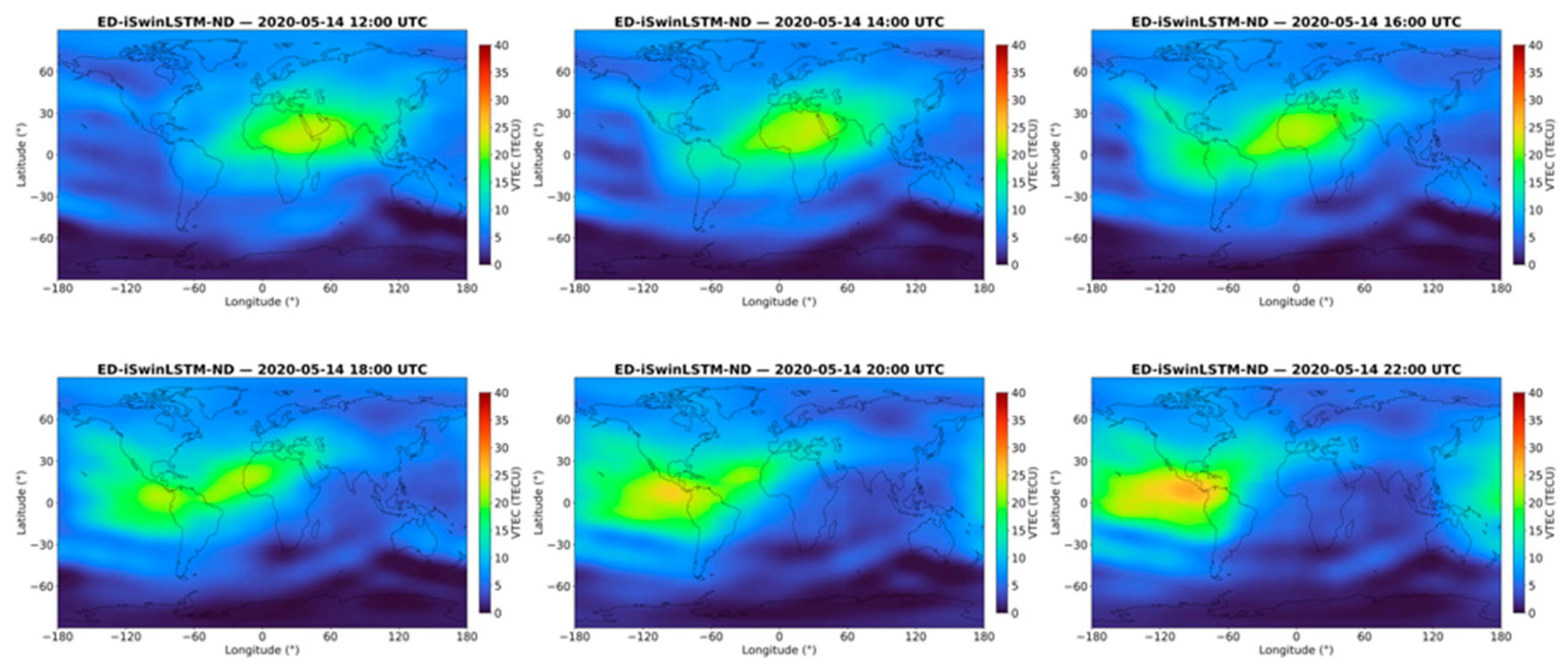
Liu et al. evaluated global TEC forecasting performance separately under geomagnetically quiet and storm-time conditions and examined its variation with forecast lead time [24]. Complementing the aggregate statistical evaluation above, this study further examined two representative cases: 1 January 2025 and 14 May 2020. A G4 (Severe) geomagnetic storm occurred on the former date [25], whereas the latter was identified as one of the five internationally quietest days of that month [26]. The global VTEC forecasts for these two cases were compared to examine how well the models reproduced the major spatial structures and to characterize their spatial error distributions, providing case-based insights that complement the aggregate statistics. By comparing the global VTEC forecasting results under storm-time and quiet geomagnetic conditions, the adaptability of the model to different ionospheric states can be further evaluated.
As shown in Figure 12 and Figure 13, the proposed model was able to reproduce the overall spatial distribution characteristics of global VTEC, including the major high- and low-value regions, under both geomagnetic activity conditions, demonstrating good forecasting capability. It can also be observed that high VTEC values are mainly concentrated in equatorial and low-latitude regions, where relatively large prediction errors are also primarily distributed. This may be attributed to complex ionospheric dynamic processes in these regions, such as the Equatorial Ionization Anomaly (EIA), where VTEC exhibits pronounced spatial gradients and strong temporal variability, thereby increasing the difficulty of accurately predicting local spatial details. Overall, even under strong geomagnetic disturbance conditions, the proposed model is still able to capture the major spatial structures of global VTEC and their variation characteristics, demonstrating stable forecasting behavior under the storm-time and quiet conditions examined.
Figure 12.
Prediction maps for 1 January 2025.
Figure 13.
Prediction maps for 14 May 2020.
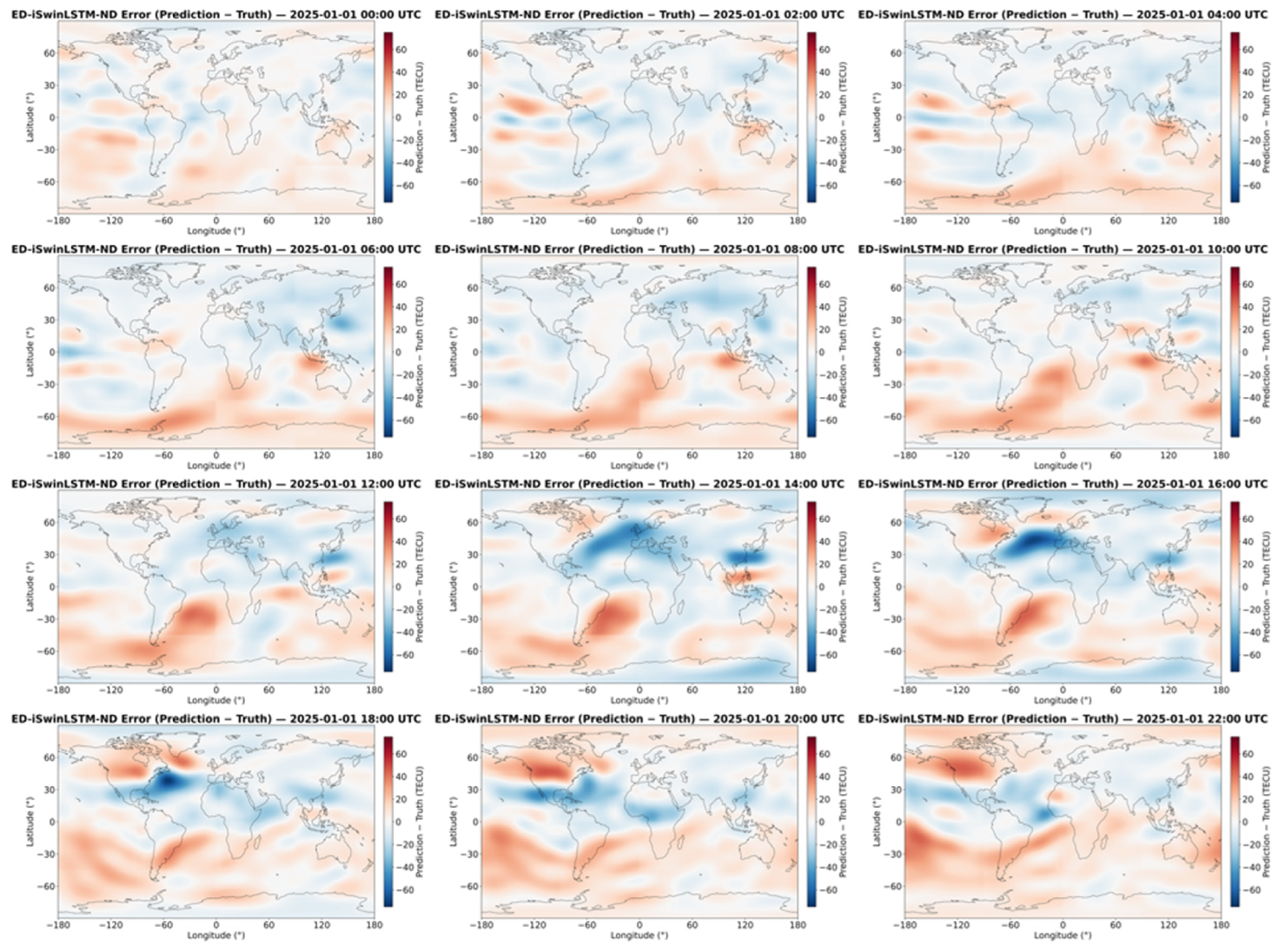
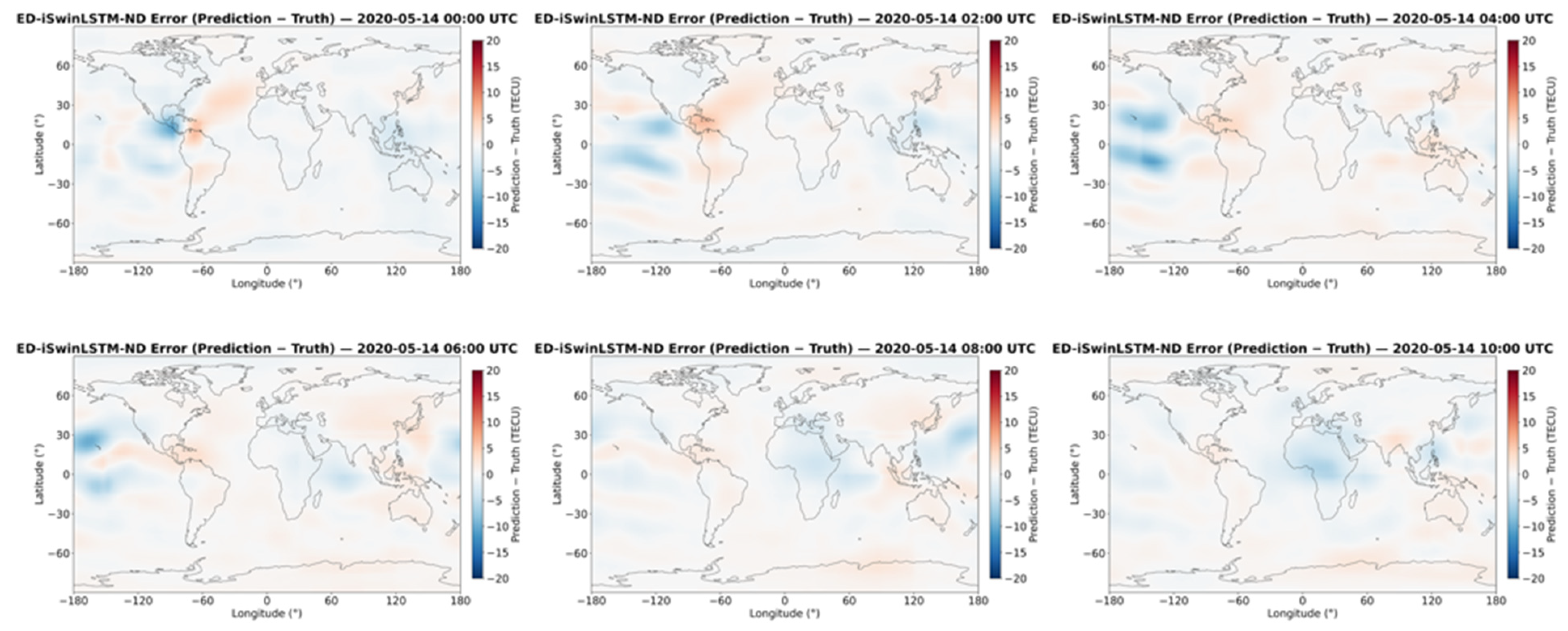
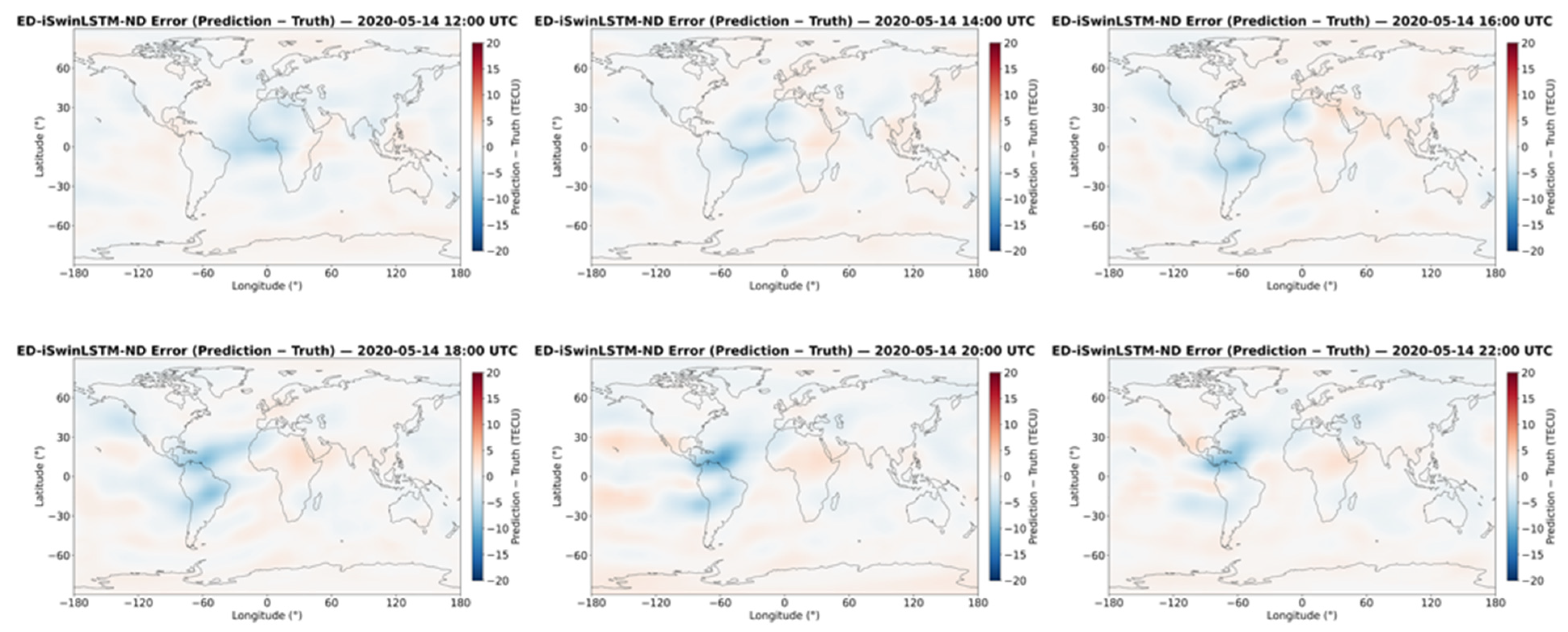
To further evaluate the forecasting performance of the model under different geomagnetic activity conditions, 1 January 2025 during a geomagnetic storm period and 14 May 2020 during a geomagnetically quiet period, were selected for a comparative analysis of the spatial distribution of global TEC prediction errors and their temporal evolution. As shown in Figure 12 and Figure 13, the model was able to preserve the major spatial variation characteristics of global TEC under both geomagnetic activity conditions, although clear differences could be observed in the magnitude and spatial distribution of the prediction errors.
During the geomagnetic storm on 1 January 2025, the overall magnitude of the prediction errors increased markedly, and the errors were distributed over a broader spatial range. Across the UTC times shown in Figure 14, pronounced positive and negative error regions were observed in some low- and mid-latitude areas, as well as in parts of the high-latitude regions. This indicates that under geomagnetic storm conditions, strong ionospheric disturbances lead to more complex spatial structures and temporal evolution of global TEC, thereby increasing the difficulty of accurately capturing rapid local variations and large-scale disturbance patterns. Nevertheless, the model generally maintains spatially continuous prediction results without obvious large-scale anomalous distortions.
Figure 14.
Prediction error maps for 1 January 2025.
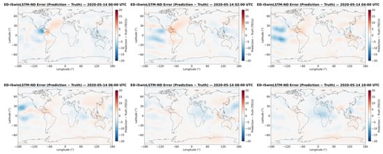
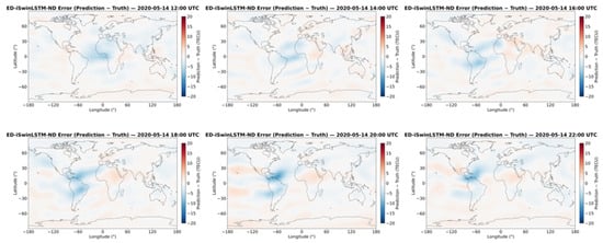
In contrast, during the geomagnetically quiet period on 14 May 2020, the overall prediction errors were substantially smaller and their spatial distributions were more concentrated. At most of the UTC times shown in Figure 15, the prediction errors remained relatively small and exhibited smoother spatial variations, with only localized positive and negative deviations in some regions. This suggests that under weak geomagnetic activity and relatively stable ionospheric conditions, the spatiotemporal variations of TEC are more regular, allowing the model to achieve higher forecasting accuracy.
Figure 15.
Prediction error maps for 14 May 2020.
Overall, the comparison between the two cases shows that geomagnetic activity has a pronounced influence on both the magnitude and spatial distribution of global TEC prediction errors. Compared with the quiet period, the prediction errors during the geomagnetic storm were not only larger overall, but also spatially more complex, indicating that intense ionospheric disturbances impose greater demands on the model’s spatiotemporal feature extraction and multi-step forecasting capabilities. In general, ED-iSwinLSTM-ND maintained relatively low prediction errors during quiet conditions and was still able to preserve the major spatial structures of global TEC under strongly disturbed conditions such as geomagnetic storms, a certain degree of stability in the representative disturbed and quiet scenarios considered.
5. Discussion
This study proposes a global TEC forecasting model, ED-iSwinLSTM-ND, based on an encoder–decoder architecture. The model extracts spatiotemporal features from 36 historical TEC maps and sequentially predicts 12 future TEC maps. Within this framework, iSwinLSTM is designed to enhance information exchange across the longitudinal boundaries of global TEC maps, while the ND strategy supplies previous-day TEC maps at corresponding times as references for next-day prediction. These components address complementary aspects of the forecasting task: spatial relationships across the map boundary and temporal correspondence between consecutive days.
Data from 2019 and 2024 were used for model training, while data from 2020 and 2025 were used for testing under low and high solar activity conditions, respectively. ED-iSwinLSTM-ND achieved the lowest aggregate MAE and RMSE among the evaluated models, including C1PG, in both test years. The stepwise results also showed comparatively low errors over lead times ranging from 2 to 24 h, although the advantage over individual competing models varied with lead time. These findings support the accuracy of the combined framework within the evaluated prediction horizon, without implying that it outperforms every competing model at every prediction step.
The boundary evaluation further shows that iSwinLSTM produced lower MAE and RMSE than SwinLSTM at both longitudinal boundaries in both test years, accompanied by lower global errors. This pattern supports the use of longitudinal periodicity in the shifted-window mechanism to improve forecasting near the map boundaries while also achieving an overall accuracy gain. Taken together, these results support the effectiveness of the proposed framework for 24-h global TEC forecasting in the two test years. Their interpretation should, however, take into account the data-availability assumptions of the experimental setup.
The evaluation uses archived GIM sequences and assumes that all historical maps required by the encoder and ND decoder are available. Although these maps precede the target interval in timestamp, their publication latency was not considered. In an operational setting, delays in obtaining the latest GIMs could leave the encoder sequence or the previous-day reference incomplete at the intended forecast issuance time. Accordingly, the reported 2–24 h lead times are measured from the epoch of the final input map. The results therefore characterize predictive accuracy under the archived-data evaluation setup and do not establish real-time operational capability. Such capability requires a separate evaluation that accounts for data availability, publication latency, and input completeness at each forecast issuance time.
6. Conclusions
To address the complex spatiotemporal variations of global TEC and the longitudinal boundary effect introduced by its two-dimensional representation, this study proposes a global TEC forecasting model, ED-iSwinLSTM-ND, based on an encoder–decoder architecture. The model employs iSwinLSTM to enhance the modeling of global TEC spatiotemporal features and longitudinal continuity, and introduces the ND strategy to incorporate TEC information from the previous day to assist future sequence forecasting. In this way, the model uses 36 historical TEC maps to sequentially predict the next 12 TEC maps. Based on experiments conducted under different solar activity conditions, the following conclusions are obtained:
- Under both high and low solar activity conditions, ED-iSwinLSTM-ND demonstrates better overall forecasting performance than LSTM, ConvLSTM, SwinLSTM, and the other encoder–decoder-based comparison models, achieving lower MAE and RMSE values and a higher R2. Compared with C1PG, the one-day TEC prediction product provided by CODE, the proposed model also exhibits higher forecasting accuracy, indicating that it can effectively learn the spatiotemporal evolution patterns of global TEC;
- iSwinLSTM improves the shifted-window mechanism by explicitly accounting for the periodic continuity of global TEC maps across the ±180° longitude boundary. The boundary experiments show that under both high and low solar activity conditions, iSwinLSTM achieved lower prediction errors than SwinLSTM at both the left and right boundaries. These results indicate that the proposed method enhances information interaction across the longitudinal boundary and effectively mitigates the boundary effect introduced by the two-dimensional representation of global TEC maps;
- The stepwise forecasting results show that ED-iSwinLSTM-ND maintains relatively stable forecasting performance over lead times ranging from 2 to 24 h. Clear differences in forecasting errors were observed among the models under different solar activity conditions, with the forecasting task generally being more challenging under high solar activity than under low solar activity. Nevertheless, the proposed model still demonstrates good forecasting accuracy and stability.
The proposed ED-iSwinLSTM-ND framework combines spatiotemporal modeling, longitudinal periodicity, and previous-day reference information for global TEC forecasting. However, the cross-solar-activity experiments reveal a marked deterioration in forecasting performance when transferring from a low-activity year to a high-activity year, while the limited year pairs currently evaluated are insufficient to establish long-term generalization capability. Future work will conduct experiments spanning at least one complete solar cycle, approximately 11 years, to systematically assess forecasting performance across different activity phases and generalization between them, and to investigate whether training on data from multiple phases can improve forecasting stability. Future work will investigate the incorporation of solar and geomagnetic activity parameters to improve the representation of disturbed ionospheric conditions. Our research group is currently receiving and processing real-time data streams in preparation for subsequent forecasting experiments. Building on this work, the next stage will evaluate the framework using inputs available at each forecast issuance time, with explicit consideration of data latency, input completeness, and processing time.
Author Contributions
Conceptualization, X.L. and F.W.; methodology, F.W.; software, F.W.; validation, F.W., L.Z. and H.T.; formal analysis, F.W.; investigation, F.W. and W.L.; resources, F.W. and K.S.; data curation, F.W. and W.M.; writing—original draft preparation, F.W.; writing—review and editing, F.W., L.Z. and H.T.; visualization, F.W. and S.L.; supervision, F.W., W.L., K.S. and W.M.; project administration, X.L.; funding acquisition, X.L. All authors have read and agreed to the published version of the manuscript.
Funding
This research was funded by the National Natural Science Foundation of China (grant number 42271461).
Data Availability Statement
The global ionospheric TEC data used in this study, including the IGS Global Ionospheric Maps (GIMs) used for model training and evaluation and the C1PG one-day-ahead predicted TEC products used for comparison, were obtained from the Crustal Dynamics Data Information System (CDDIS) archive. These data are publicly available at https://cddis.nasa.gov/archive/gnss/products/ionex/ (accessed on 21 May 2026). We thank CDDIS, the International GNSS Service (IGS), and the Center for Orbit Determination in Europe (CODE) for providing the ionospheric data products used in this study.
Acknowledgments
The authors of this paper would like to thank the reviewers for their careful review and their invaluable revisions, which have improved its presentation.
Conflicts of Interest
The authors declare no conflicts of interest.
Abbreviations
The following abbreviations are used in this manuscript:
| TEC | Total Electron Content |
| VTEC | Vertical Total Electron Content |
| GNSS | Global Navigation Satellite System |
| GIM | Global Ionospheric Map |
| IONEX | IONosphere Map EXchange |
| IRI | International Reference Ionosphere |
| ARMA | Autoregressive Moving Average |
| ARIMA | Autoregressive Integrated Moving Average |
| MLP | Multilayer Perceptron |
| LSTM | Long Short-Term Memory |
| ED-LSTM | Encoder–Decoder Long Short-Term Memory |
| ConvLSTM | Convolutional Long Short-Term Memory |
| SwinLSTM | Swin Transformer-based Long Short-Term Memory |
| ED | Encoder–Decoder |
| ND | Next-Day |
| MAE | Mean Absolute Error |
| RMSE | Root Mean Square Error |
| R2 | Coefficient of Determination |
| IGS | International GNSS Service |
| CODE | Center for Orbit Determination in Europe |
| C1PG | CODE 1-Day Predicted Global Ionospheric Map |
| IAAC | Ionosphere Associate Analysis Center |
References
- Sanz Subirana, J.; Juan Zornoza, J.M.; Hernández-Pajares, M. GNSS Data Processing, Volume I: Fundamentals and Algorithms; ESA TM-23/1; ESA Communications: Noordwijk, The Netherlands, 2013. [Google Scholar]
- Kintner, P.M.; Ledvina, B.M. The ionosphere, radio navigation, and global navigation satellite systems. Adv. Space Res. 2005, 35, 788–811. [Google Scholar] [CrossRef] [Scilit]
- Rovira-Garcia, A.; Juan, J.M.; Sanz, J.; González-Casado, G. A worldwide ionospheric model for fast precise point positioning. IEEE Trans. Geosci. Remote Sens. 2015, 53, 4596–4604. [Google Scholar] [CrossRef] [Scilit]
- Jakowski, N.; Béniguel, Y.; De Franceschi, G.; Hernández-Pajares, M.; Jacobsen, K.S.; Stanislawska, I.; Tomasik, L.; Warnant, R.; Wautelet, G. Monitoring, tracking and forecasting ionospheric perturbations using GNSS techniques. J. Space Weather Space Clim. 2012, 2, A22. [Google Scholar] [CrossRef] [Scilit]
- Schunk, R.W. A Mathematical Model of the Middle and High Latitude Ionosphere. Pure Appl. Geophys. 1988, 127, 255–303. [Google Scholar] [CrossRef] [Scilit]
- Fuller-Rowell, T.J.; Rees, D.; Quegan, S.; Bailey, G.J.; Moffett, R.J. Interactions between Neutral Thermospheric Composition and the Polar Ionosphere Using a Coupled Ionosphere–Thermosphere Model. J. Geophys. Res. 1987, 92, 7744–7748. [Google Scholar] [CrossRef] [Scilit]
- Ridley, A.J.; Deng, Y.; Tóth, G. The Global Ionosphere–Thermosphere Model. J. Atmos. Sol.-Terr. Phys. 2006, 68, 839–864. [Google Scholar] [CrossRef] [Scilit]
- Bilitza, D. International Reference Ionosphere: Recent Developments. Radio Sci. 1986, 21, 343–346. [Google Scholar] [CrossRef] [Scilit]
- Bilitza, D. International Reference Ionosphere 2000. Radio Sci. 2001, 36, 261–275. [Google Scholar] [CrossRef] [Scilit]
- Bilitza, D.; Altadill, D.; Truhlik, V.; Shubin, V.; Galkin, I.; Reinisch, B.; Huang, X. International Reference Ionosphere 2016: From Ionospheric Climate to Real-Time Weather Predictions. Space Weather 2017, 15, 418–429. [Google Scholar] [CrossRef] [Scilit]
- Hochegger, G.; Nava, B.; Radicella, S.; Leitinger, R. A Family of Ionospheric Models for Different Uses. Phys. Chem. Earth Part C Sol. Terr. Planet. Sci. 2000, 25, 307–310. [Google Scholar] [CrossRef] [Scilit]
- Nava, B.; Coïsson, P.; Radicella, S.M. A New Version of the NeQuick Ionosphere Electron Density Model. J. Atmos. Sol.-Terr. Phys. 2008, 70, 1856–1862. [Google Scholar] [CrossRef] [Scilit]
- Bent, R.B.; Llewellyn, S.K.; Nesterczuk, G.; Schmid, P.E. The Development of a Highly-Successful Worldwide Empirical Ionospheric Model and Its Use in Certain Aspects of Space Communications and Worldwide Total Electron Content Investigations. In Effect of the Ionosphere on Space Systems and Communications; Naval Research Laboratory: Washington, DC, USA, 1975; Volume 1, pp. 13–28. [Google Scholar]
- Ratnam, D.V.; Otsuka, Y.; Sivavaraprasad, G.; Dabbakuti, J.R.K.K. Development of Multivariate Ionospheric TEC Forecasting Algorithm Using Linear Time Series Model and ARMA over Low-Latitude GNSS Station. Adv. Space Res. 2019, 63, 2848–2856. [Google Scholar] [CrossRef] [Scilit]
- Mandrikova, O.V.; Fetisova, N.V.; Al-Kasasbeh, R.T.; Klionskiy, D.M.; Geppener, V.V.; Ilyash, M.Y. Ionospheric Parameter Modelling and Anomaly Discovery by Combining the Wavelet Transform with Autoregressive Models. Ann. Geophys. 2015, 58, A0550. [Google Scholar] [CrossRef] [Scilit]
- Ansari, K.; Park, K.-D.; Kubo, N. Linear Time-Series Modeling of the GNSS-Based TEC Variations over Southwest Japan during 2011–2018 and Comparison against ARMA and GIM Models. Acta Astronaut. 2019, 165, 248–258. [Google Scholar] [CrossRef] [Scilit]
- Akhoondzadeh, M. A MLP Neural Network as an Investigator of TEC Time Series to Detect Seismo-Ionospheric Anomalies. Adv. Space Res. 2013, 51, 2048–2057. [Google Scholar] [CrossRef] [Scilit]
- Hochreiter, S.; Schmidhuber, J. Long Short-Term Memory. Neural Comput. 1997, 9, 1735–1780. [Google Scholar] [CrossRef] [Scilit] [PubMed]
- Sun, W.; Xu, L.; Huang, X.; Zhang, W.; Yuan, T.; Chen, Z.; Yan, Y. Forecasting of Ionospheric Vertical Total Electron Content (TEC) Using LSTM Networks. In Proceedings of the 2017 International Conference on Machine Learning and Cybernetics (ICMLC), Ningbo, China, 9–12 July 2017; IEEE: Piscataway, NJ, USA, 2017; Volume 2, pp. 340–344. [Google Scholar] [CrossRef] [Scilit]
- Xiong, P.; Zhai, D.; Long, C.; Zhou, H.; Zhang, X.; Shen, X. Long Short-Term Memory Neural Network for Ionospheric Total Electron Content Forecasting over China. Space Weather 2021, 19, e2020SW002706. [Google Scholar] [CrossRef] [Scilit]
- Liu, Z.; Lin, Y.; Cao, Y.; Hu, H.; Wei, Y.; Zhang, Z.; Lin, S.; Guo, B. Swin Transformer: Hierarchical Vision Transformer Using Shifted Windows. In Proceedings of the IEEE/CVF International Conference on Computer Vision (ICCV), Montreal, QC, Canada, 10–17 October 2021; IEEE: Piscataway, NJ, USA, 2021; pp. 10012–10022. [Google Scholar] [CrossRef] [Scilit]
- Tang, S.; Li, C.; Zhang, P.; Tang, R. SwinLSTM: Improving Spatiotemporal Prediction Accuracy Using Swin Transformer and LSTM. In Proceedings of the IEEE/CVF International Conference on Computer Vision (ICCV), Paris, France, 1–6 October 2023; IEEE: Piscataway, NJ, USA, 2023; pp. 13470–13479. [Google Scholar] [CrossRef] [Scilit]
- Li, M.; Yuan, Y.; Wang, N.; Li, Z.; Huo, X. Performance of Various Predicted GNSS Global Ionospheric Maps Relative to GPS and JASON TEC Data. GPS Solut. 2018, 22, 55. [Google Scholar] [CrossRef] [Scilit]
- Liu, L.; Morton, Y.J.; Liu, Y. ML Prediction of Global Ionospheric TEC Maps. Space Weather 2022, 20, e2022SW003135. [Google Scholar] [CrossRef] [Scilit]
- NESDIS Secures Timely Data to Help Safeguard Earth’s Rhythms in the New Year. Available online: https://www.nesdis.noaa.gov/news/nesdis-secures-timely-data-help-safeguard-earths-rhythms-the-new-year (accessed on 4 September 2026).
- Monthly Overview: May 2020. Available online: https://www.kakioka-jma.go.jp/obsdata/overview/overview_month_en/2020/5 (accessed on 4 September 2026).



Disclaimer/Publisher’s Note: The statements, opinions and data contained in all publications are solely those of the individual author(s) and contributor(s) and not of MDPI and/or the editor(s). MDPI and/or the editor(s) disclaim responsibility for any injury to people or property resulting from any ideas, methods, instructions or products referred to in the content. |
© 2026 by the authors. Licensee MDPI, Basel, Switzerland. This article is an open access article distributed under the terms and conditions of the Creative Commons Attribution (CC BY) license.