Lake Water Color Dynamics, Environmental Drivers, and Optical Responses in Arid Northwest China: A 42-Year Landsat-Based Analysis

Highlights

What are the main findings?

• Landsat-derived hue angles for 350 lakes (1984–2025) revealed strong spatial heterogeneity and a sustained decline over the past 42 years in lake water color across arid Northwest China.
• Three water-color phenological types—Aseasonal (75.0%), Summer Greening (13.7%), and Spring Greening (11.3%)—were identified, and color resilience increased in 43% of lakes but declined in 21%, which clustered at 37–43°N and 83–89°E.

What are the implications of the main findings?

• Lake morphology was the strongest correlate of water color, topography and thermal conditions were most associated with phenology, and watershed population dynamics ranked highest for resilience, suggesting that conserving arid-zone lakes under climate warming may depend on stabilizing human pressure as much as on natural setting.
• Hue angle co-varied with optically active constituents and DOM composition, indicating its potential as an integrative water-quality indicator for targeted long-term satellite monitoring and adaptive watershed management in climate-sensitive arid regions.

Abstract

Lake water color provides an integrated indicator of aquatic environmental change, yet its long-term phenology and resilience remain poorly understood in arid regions. In this study, Landsat-derived hue angle (α) records were reconstructed for 350 lakes larger than 1 km² across arid Northwest China from 1984 to 2025. Regional mean α declined significantly over the past 42 years (R² = 0.51), accompanied by pronounced spatial heterogeneity. Three lake water color phenological types were identified: Aseasonal (75.0%), Summer Greening (13.7%), and Spring Greening (11.3%). Aseasonal lakes were the most stable, whereas seasonal lakes showed greater temporal variability and a tendency to transition toward aseasonality. Lake water color resilience increased in 43% of lakes, declined in 21%, and remained unchanged in 36%, with resilience-loss lakes showing distinct spatial clustering. Lake morphology was most strongly associated with water color change, topography and thermal conditions with its phenology, and watershed population dynamics with its resilience. In situ observations further showed significant relationships between α and optically active constituents and their derived parameters, reflecting the combined optical effects of absorption and scattering and suggesting its potential as a proxy for broader water-quality assessment with more extensive field sampling and validation. These findings highlight contrasting controls on lake-color dynamics, phenology, and resilience, and demonstrate the value of hue angle for monitoring environmental change in vulnerable arid-zone lakes. Overall, these results advance understanding of the long-term environmental responses of arid-zone lakes and provide a scientific basis for targeted monitoring and adaptive management in arid regions.

1. Introduction

Lakes are vital components of inland water systems, supporting aquatic biodiversity and contributing to global carbon cycling and climate regulation. However, climate change and human activities have substantially altered lake environments worldwide [1,2,3,4], leading to increased carbon burial [5,6], deoxygenation [7], cyanobacterial blooms [8,9], and shifts in water color associated with changes in phytoplankton, oxygen conditions, and nutrient cycling [5,10,11]. Water color therefore serves as an integrated indicator of lake environmental condition, while its seasonal phenology and resilience derived from long-term color time series provide additional information on seasonal dynamics and responses to disturbance. This is particularly important in arid Northwest China, where lakes are highly vulnerable to limited precipitation, dependence on alpine meltwater, intensive upstream water withdrawal, and rapid hydrological change, with widespread shrinkage, salinization, and drying already reported [12,13,14], in contrast to the satellite-observed surface-water gains in lake-rich high-latitude regions [15]. Because such degradation can further affect regional water security and enhance dust emissions from exposed saline lakebeds [16], and because long-term ground observations remain sparse, systematic satellite monitoring of water-color dynamics, phenology, and resilience is essential for understanding environmental change and assessing the condition of these vulnerable lakes.

With advantages in large-scale coverage, cost efficiency, and continuous observation, satellite remote sensing has become a widely used approach for water-color monitoring, commonly characterized by metrics such as the Forel–Ule index, hue angle (α), and dominant wavelength. Accordingly, satellite-based studies of lake water color have expanded from individual lakes, such as Qinghai Lake [17], to national-scale assessments across China [18,19], while regional studies have further revealed spatiotemporal and seasonal patterns in the Yangtze River Basin [20], urban lake systems [21], and the Tibetan Plateau [22]. Water-color phenology and transitions among phenological patterns have also been investigated to characterize seasonal lake dynamics [23,24]. In addition, lake resilience has been assessed using other indicators [25], including disturbance–recovery capacity [26], hierarchical drought impacts [27], and long-term shifts in biological communities [28]. Among these water-color metrics, hue angle provides a continuous representation of water color, enabling finer and more objective characterization of subtle optical variations [29,30,31]. Meanwhile, a decrease in the hue angle indicates a shift towards bluer water with lower chroma, signifying ecological implications such as lower constituent loads and a reduced contribution of terrestrial dissolved organic matter [29,30,32,33]. Despite these advances, continuous hue-angle monitoring remains scarce in arid Northwest China [34], where long-term water-color dynamics, common seasonal phenological patterns, and water-color resilience have yet to be systematically characterized.

Beyond describing water-color patterns, phenology, and resilience, interpreting the environmental processes underlying these variations is equally important. Linking water-color dynamics to climatic, terrestrial, and anthropogenic factors can help clarify the mechanisms driving long-term lake change and distinguish the relative roles of natural and human pressures [35]. At the same time, because water color integrates the optical effects of multiple water constituents, its potential as a proxy for other water-quality properties has been increasingly recognized [32], with relationships reported for chlorophyll-a, suspended matter, transparency [36,37], and colored dissolved organic matter [33], among others. However, these relationships depend strongly on the composition and relative contributions of optically active constituents and may vary among lake types [29,38]. This is particularly relevant for arid Northwest China, where high suspended sediment loads, salinity, mineral precipitation, and terrestrial inputs can generate optical conditions distinct from those of humid and eutrophic lakes [39,40]. It is therefore necessary to examine both the environmental drivers of water-color dynamics and their relationships with water-quality parameters, so as to evaluate the broader applicability of water color and clarify the underlying optical mechanisms in arid inland lakes.

In this study, Landsat Collection 2 Level-2 products were processed via Google Earth Engine (GEE) to retrieve hue angle time series from 1984 to 2025 for 350 lakes larger than 1 km² across arid Northwest China. Based on these time series, the spatiotemporal patterns of lake water color were characterized, dominant phenological types and their transitions were identified, and water-color resilience was assessed within an early warning signals framework. The key drivers of lake water-color dynamics were further investigated, and water-quality measurements from collected samples were used to examine the relationships between hue angle (α) and other water-quality parameters, thereby evaluating its potential for broader water-quality assessment. This study provides a long-term, region-wide perspective on lake environmental dynamics and establishes a basis for understanding environmental change, identifying emerging risks, and elucidating the responses of vulnerable arid-zone lakes to climatic and anthropogenic pressures.

2. Materials and Methods

2.1. Study Area

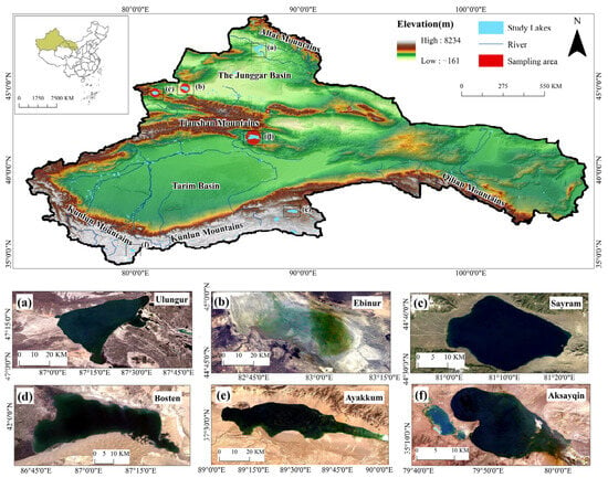
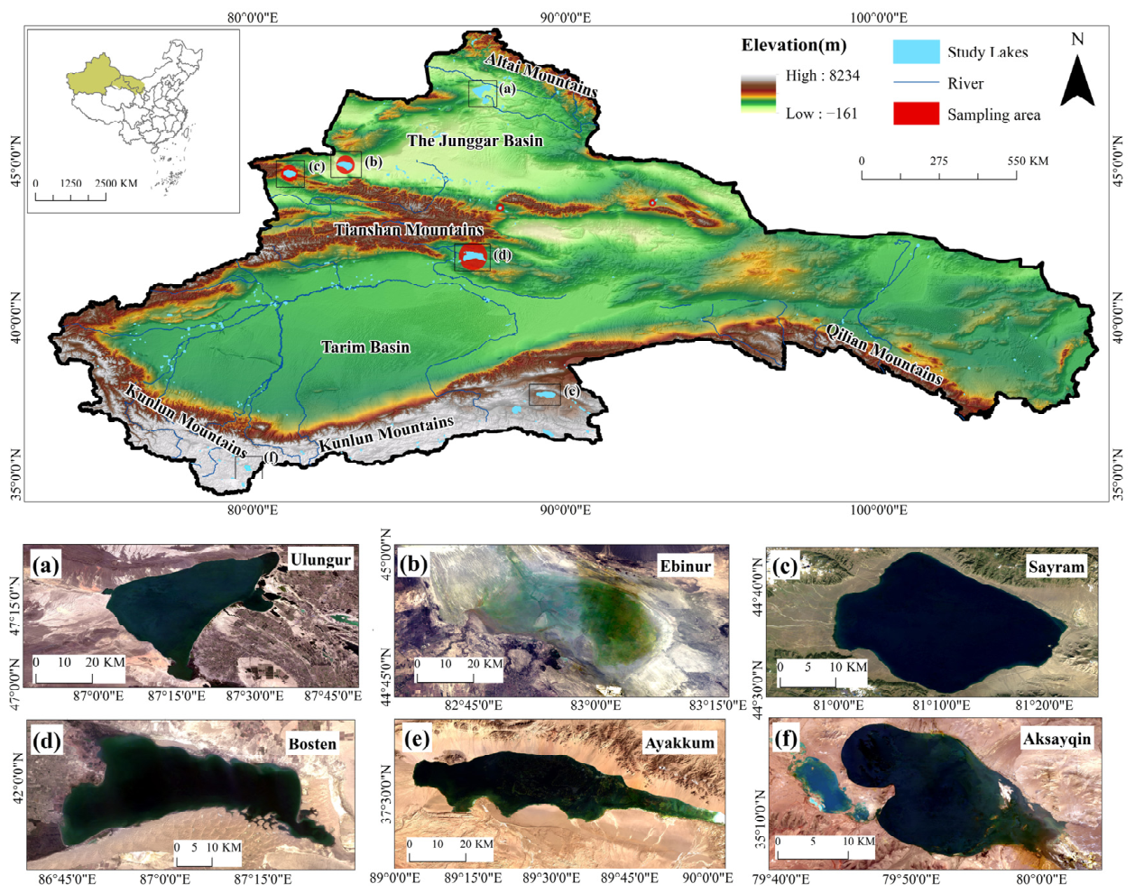
The arid region of Northwest China is located between 35–50°N and 73–106°E, spanning the administrative areas of Shaanxi Province, Ningxia Hui Autonomous Region, Gansu Province, Qinghai Province, and Xinjiang Uygur Autonomous Region (Figure 1). The topography and geomorphology of this region are extremely complex, characterized by a macro-scale pattern of towering mountain ranges alternating with vast basins [41]. Climatically, the region falls under a typical temperate continental climate [42], marked by scarce precipitation and high evaporation. The unique topographic and climatic conditions collectively result in sparse vegetation with low coverage, dominated mainly by deserts and sandy lands [43]. Lakes are generally scarce in arid Northwest China, with a total of 350 lakes larger than 1 km², most of which are located in the Xinjiang Uygur Autonomous Region. They are primarily distributed in the Junggar Basin and along the southern foothills of the Altai Mountains in northern Xinjiang, represented by Ulungur Lake and Ebinur Lake; along the central and western Tianshan Mountains and within adjacent intermountain basins, represented by Sayram Lake and Bosten Lake; and in the high-altitude basins of the Kunlun–Altun mountain region in southern Xinjiang, represented by Ayakkum Lake and Aksayqin Lake (Figure 1a–f). The fundamental characteristics of lake development in this region are a small number of lakes, diverse types, and complex structures, encompassing categories such as salt lakes, saline lakes, brackish lakes, and freshwater lakes, making it a representative area for research on arid zone lake systems.

Figure 1. Spatial distribution of 350 lakes larger than 1 km² in the arid region of Northwest China, with six typical lakes shown in panels (a–f).

2.2. Datasets

2.2.1. Satellite Data

To obtain long-term satellite observations of lake water color and exclude the influence of ice-covered periods, this study used the Landsat Collection 2 Level-2 surface reflectance dataset provided by the GEE platform. The data period covered March to October of each year from 1984 to 2025, totaling 57,464 scenes, mainly including Landsat 5 Thematic Mapper (TM), Landsat 7 Enhanced Thematic Mapper Plus (ETM+), and Landsat 8 Operational Land Imager (OLI) imagery. All images have a spatial resolution of 30 m and a revisit cycle of 16 days, and have undergone radiometric and geometric correction, constituting high-quality data products. The DN values were converted to surface reflectance according to the Collection 2 calibration coefficients, and scenes with scene-level cloud cover greater than 80% were excluded, ensuring data reliability. Clouds, cloud shadows, and snow/ice were removed using the QA_PIXEL quality band (bits 3, 4, and 5), and imagery from March to October was selected to further minimize ice and snow cover. Water pixels were extracted using the normalized difference water index (NDWI), while algae-contaminated pixels were excluded via the floating algae index (FAI). Hue angles were constrained to 0–360° to discard invalid values. For the Landsat 7 ETM+ imagery, only 2013 data were used; the SLC-off data gaps are flagged as no-data in the Collection 2 Level-2 product and were excluded by the quality mask [44].

2.2.2. In Situ Sampling Data

This study utilized water quality parameters from several representative lakes (Barkol Lake, Bosten Lake, Chaiwopu Lake, Ebinur Lake, and Sayram Lake) for the influencing factor analysis. Field sampling was carried out in two campaigns, in August 2018 and in June–August 2025, during the ice-free season; surface water samples were collected at a depth of about 0.5 m. The parameters were determined as follows. Conductivity (Cond), salinity (Sal), and total dissolved solids (TDS) were measured in situ with an SL1000 portable multi-parameter water quality analyzer (Hach, Loveland, CO, USA), and transparency (SD) was measured in situ with a Secchi disk; among the eight major ions, anions (Cl⁻, SO₄²⁻) were determined by ion chromatography (ICS-5000, Thermo Fisher Scientific, Waltham, MA, USA), cations (Ca²⁺, Mg²⁺, K⁺, Na⁺) by inductively coupled plasma optical emission spectrometry (735 ICP-OES, Agilent Technologies, Santa Clara, CA, USA), and CO₃²⁻ and HCO₃⁻ by potentiometric titration (G20, Mettler-Toledo, Greifensee, Switzerland); chlorophyll-a (Chl-a) was determined by hot-ethanol extraction, total nitrogen (TN) by digital titrimetry, and total phosphorus (TP) by the molybdenum-blue method, all measured with a UV spectrophotometer (UV-3600 Plus, Shimadzu, Kyoto, Japan); total suspended matter (TSM) was determined by the gravimetric method; dissolved organic carbon (DOC) and total carbon (TC) were determined by combustion oxidation with a total organic carbon analyzer (TOC-L, Shimadzu, Kyoto, Japan); the CDOM absorption coefficient aCDOM(350) was determined by spectrophotometry; chemical oxygen demand (COD) was measured by the potassium permanganate oxidation method; and dissolved organic matter fluorescence was characterized by three-dimensional excitation–emission matrices (EEMs) measured with a Horiba Aqualog fluorescence spectrometer (Horiba Scientific, Edison, NJ, USA), from which the ratio of humic-like to protein-like fluorescence intensity (H:P), the ratio of the fluorescence integrals of peak C to peak T (IC:IT), and the humification index (HIX) were derived. To match in situ sampling with satellite observations for three typical lakes (Bosten Lake, Ebinur Lake, and Sayram Lake), the nearest valid Landsat 8 Collection 2 Level-2 image within 1 day of each sampling date was selected on GEE, and the spectral reflectance and hue angle were extracted from valid pixels. Specifically, reflectance was taken as the median of valid pixels within a 45 m buffer around each site; after masking clouds, cloud shadows, and snow/ice, only sites containing at least one valid pixel were retained.

2.2.3. Auxiliary Data

To explore the various driving factors, this study extracted lake attribute data from the HydroLAKES database v1.0 [45], including shoreline length, shoreline development coefficient, water storage, depth, discharge, water renewal time, elevation, surrounding slope, watershed area, and lake-to-watershed area ratio. In addition, climatic, landscape, and population data were incorporated. Specifically, annual mean air temperature and monthly precipitation for 1984–2024 were obtained from the China 1-km annual mean air temperature dataset and the 1-km monthly precipitation dataset [46], respectively; 10 m wind speed for 1984–2024 was obtained from the China Meteorological Forcing Dataset (CMFD) at approximately 10 km (0.1°) resolution; and the 250 m annual NDVI for 2000–2024 was generated from monthly products using the maximum value composite method. All these data were provided by the National Tibetan Plateau Data Center (https://data.tpdc.ac.cn/home); population density at approximately 1 km resolution for 2000–2024 was obtained from the LandScan dataset provided by Oak Ridge National Laboratory (https://landscan.ornl.gov, accessed on 30 August 2025). For each lake, all raster variables were spatially aggregated by zonal averaging within its corresponding watershed to obtain a single representative value; the coefficients of variation for annual mean air temperature, monthly precipitation, wind speed, NDVI, and population density were also calculated as derived variables of the influencing factors.

2.3. Method

2.3.1. Derivation of Hue Angle

The hue angle α characterizes the direction of color in chromaticity space, reflecting its hue [47]. Its calculation first converts visible-band reflectance into the CIE-XYZ tristimulus values X, Y, and Z. Since TM and ETM+ have only three visible bands, the RGB conversion formula (Equation (1)) is adopted [48]; OLI has four visible bands and uses linear interpolation coefficients for conversion (Equation (2)) [30]. After normalizing the tristimulus values to CIE-xy chromaticity coordinates (Equation (3)), α is computed from the orientation of the chromaticity coordinates relative to the white point (1/3, 1/3) following the convention of Wang et al. [49] (Equation (4)), yielding a continuous variable ranging from 0° to 360° with values increasing from deep blue through green toward reddish-brown waters. Owing to the inherent discrete nature of multispectral remote sensing imagery, systematic biases are introduced in the calculation of water hue angle, such that the results cannot be fully equivalent to those derived from hyperspectral data [50]. To correct this bias, a fifth-order polynomial ∆-correction [30,51] is applied: Equation (5) for Landsat 5 TM; Equation (6) for Landsat 7 ETM+; and Equation (7) for Landsat 8 OLI. In addition, both the strong linear relationship between the hue angle α derived in this study and the FUI product of Wang et al. [52] (R² = 0.897; Figure S1a) and the good cross-sensor consistency of α (Figure S1b,c) indicate that our α extraction is robust and reliable, thereby supporting its further application in subsequent analyses.

$$\left\{\begin{array}{l}X=2.7689R+1.7517G+1.1302B\\ Y=1.0000R+4.5907G+0.0601B\\ Z=0.0000R+0.0565G+5.5943B\end{array}\right.$$

(1)

$$\left\{\begin{array}{l}X=11.053{\rho }_{443}+6.950{\rho }_{483}+51.135{\rho }_{561}+34.457{\rho }_{655}\\ Y=1.320{\rho }_{443}+21.053{\rho }_{483}+66.023{\rho }_{561}+18.034{\rho }_{655}\\ Z=58.038{\rho }_{443}+34.931{\rho }_{483}+2.606{\rho }_{561}+0.016{\rho }_{655}\end{array}\right.$$

(2)

$$\left\{\begin{array}{l}x={\displaystyle \frac{X}{X+Y+Z}}\\ y={\displaystyle \frac{Y}{X+Y+Z}}\end{array}\right.$$

(3)

$$\alpha =\arctan 2\left(x-{\displaystyle \frac{1}{3}},\hspace{0.33em}y-{\displaystyle \frac{1}{3}}\right)\times {\displaystyle \frac{{180}^{\circ }}{\pi }}+{180}^{\circ }$$

(4)

∆ = −29.045a⁵ + 156.91a⁴ − 279.9a³ + 128.18a² + 103.81a − 34.578

(5)

∆ = −5.435a⁵ + 11.915a⁴ + 22.991a³ − 97.332a² + 120.7a − 25.977

(6)

$$∆=-52.819a^5+334.88a^4-758.26a^3+746.32a^2-315.18a+39.761, \left(a={\displaystyle \frac{\alpha }{100}}\right)$$

(7)

2.3.2. Phenological Analysis of Seasonal Lakes Water Color

First, to exclude the influence of frozen periods, only water color results from March to October each year were used to perform phenological analysis. In addition, to investigate the evolving characteristics of lake water color phenology across different periods while balancing data volume and temporal resolution, the period from 1984 to 2025 was divided into seven intervals for analysis. Within each interval, extreme outliers exceeding four standard deviations from the interval mean were removed, and the data were smoothed using Nadaraya–Watson kernel regression [53,54] with a Gaussian kernel and a bandwidth of 10 to obtain curves representing seasonal patterns. Because each lake was processed independently within each interval, the unit of phenological classification was the lake–period observation rather than the lake itself. This yielded 2155 lake–period observations across the 350 lakes for the seven intervals after removing the aforementioned outliers.

Since the seasonal phenological patterns of lake water color are not predetermined, this study employed the clustering analysis method that does not require predefined groups to identify seasonal variation patterns in the 42-year water color time series data [55,56]. To prevent lakes without seasonal patterns (Aseasonal lakes) from interfering with the identification of seasonal patterns and to enhance the stability and interpretability of clustering, an objective threshold method based on clustering stability optimization (using a standard deviation threshold of σ ≤ 15.14, which was identified as the value maximizing bootstrap clustering stability across candidate quantiles) was employed to pre-separate Aseasonal lakes. Furthermore, for the remaining time series, which were z-score normalized, hierarchical clustering based on partition clustering with centroid averaging was performed using the seasonal Dynamic Time Warping method [57], and the optimal number of clusters was determined by comprehensively evaluating the Davies–Bouldin index, silhouette coefficient, and Calinski–Harabasz index. These indices consistently supported a two-cluster solution (Davies–Bouldin = 0.67, silhouette = 0.43, Calinski–Harabasz = 703.16). Subsequently, the Jaccard similarity index calculated via bootstrap resampling was employed to assess the stability of the clustering results, with values exceeding 0.5 generally indicating that the identified water color phenological patterns are robust and true. The non-parametric Kruskal–Wallis analysis of variance [58], followed by Dunn’s test with Bonferroni correction [59], was applied to examine whether significant differences existed among the features of different clusters.

Furthermore, the phenological stability of lakes was assessed by quantifying the frequency of cluster transitions across successive intervals [23]. Subsequently, to statistically evaluate differences in stability among lakes of distinct phenological types, pairwise comparisons were performed using Dunn’s test based on mean ranks [59], calculated from retention rates across observational periods. The Bonferroni correction was applied to adjust significance levels and control for multiple comparisons [60]. Finally, by tracking each lake’s phenological type over consecutive observation periods, transition probabilities were derived by dividing the frequency of each transition pathway by the total occurrences of its starting phenological state [61]. This approach quantitatively expressed the probabilities of a lake maintaining its current phenological type or transitioning to another in the subsequent phase.

2.3.3. Lake Water Color Resilience Estimation

Lake water color resilience refers to the ability of a lake color to maintain its key functions and structure or to return to its original state after being subjected to external disturbances. Here, detrended hue angle data—processed through linear interpolation, harmonic regression to remove seasonal fluctuations, and moving average to eliminate long-term trends—were used to quantitatively measure changes in lake resilience. To mitigate potential errors from a single metric and enhance the reliability of resilience calculations, we selected four universal indicators of resilience associated with Early Warning Signals (EWS) of ecosystem services [62]: standard deviation (SD), lag-1 autocorrelation (AR), skewness (SK), and kurtosis (KT). As a system approaches a critical transition, critical slowing down not only raises SD and AR but also, through intermittent flickering between states, produces heavier-tailed and more asymmetric fluctuations, so that rising kurtosis and increasing skewness likewise indicate declining resilience [62,63]. Following sensitivity testing and to align with common standards in resilience research [63,64,65], a five-year sliding window was adopted for the calculation of lake water color resilience indicators. The time series were linearly interpolated at a monthly resolution (filling only gaps of ≤8 consecutive months), deseasonalized by a second-order harmonic regression, and detrended with a one-year centered moving average; the four indicators were then computed at each position of a five-year window advanced along the series with a one-month step. The testing results confirm that the resilience classification is robust across the tested parameter ranges (Text S1).

$$\mathit{SD}=\sqrt{{\displaystyle \frac{1}{n-1}}\sum _{t=1}^n{(z_t-\mu )}^2}$$

(8)

$$\mathit{AR}={\displaystyle \frac{{\sum }_{t=1}^{n-1}\left(z_t-\mu \right)(z_{t+1}-\mu )}{{\sum }_{t=1}^n{\left(z_t-\mu \right)}^2}}$$

(9)

$$\mathit{SK}={\displaystyle \frac{\frac{1}{n}{\sum }_{t=1}^n{\left(z_t-\mu \right)}^3}{{\left(\sqrt{\frac{1}{n}{\sum }_{t=1}^n{\left(z_t-\mu \right)}^2}\right)}^3}}$$

(10)

$$\mathit{KT}={\displaystyle \frac{\frac{1}{n}{\sum }_{t=1}^n{\left(z_t-\mu \right)}^4}{{\left(\sqrt{\frac{1}{n}{\sum }_{t=1}^n{\left(z_t-\mu \right)}^2}\right)}^4}}$$

(11)

Here, z is the detrended hue angle time series within the sliding window; μ is the mean of this series; n is the number of observations within the window; z_t+1 is the first-order lagged value; and $\sum _{t=1}^n{(z_t-\mu )}^2$ is the sum of squared deviations of the series.

Within the EWS framework, lake water color resilience was categorized based on trends in four indicators: resilience was considered to be lost if at least two indicators showed statistically significant increasing trends, to increase if at least two showed statistically significant decreasing trends (both at p < 0.05), and to remain stable in the absence of such consistent signals [62,66,67]. Because this criterion requires at least two indicators to agree in direction with fewer than two opposing, cases with no dominant direction, including two increasing and two decreasing, were classified as “No change”. In order to identify the variation trends of each indicator, the Mann–Kendall analysis [68] was employed for the analysis of their respective time series.

2.3.4. Analysis of Driving Factors and Response Relationship

The random forest method was used to rank the importance of anthropogenic, climatic, and lake-intrinsic factors affecting image-derived lake water color. The permutation-based random forest method was applied to rank the influence of the above factors on phenological type classification, and regression analysis was used to identify variables that may affect the stability of water-color phenology. For the resilience-driven analysis, we employed the non-parametric Kruskal–Wallis H test [69] to examine whether the three classes of samples originated from the same distribution, with the ε² statistic [70] to measure effect size, where ε² values of approximately 0.01, 0.06, and 0.14 denote small, medium, and large effects, respectively [71], and ranked the factors accordingly. Relationships between α and water-quality parameters were further evaluated using linear regression, with statistical significance used to determine the strength and reliability of the observed associations.

3. Results

3.1. Spatiotemporal Distribution of Lake Water Color in Arid Region of Northwest China

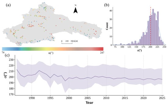
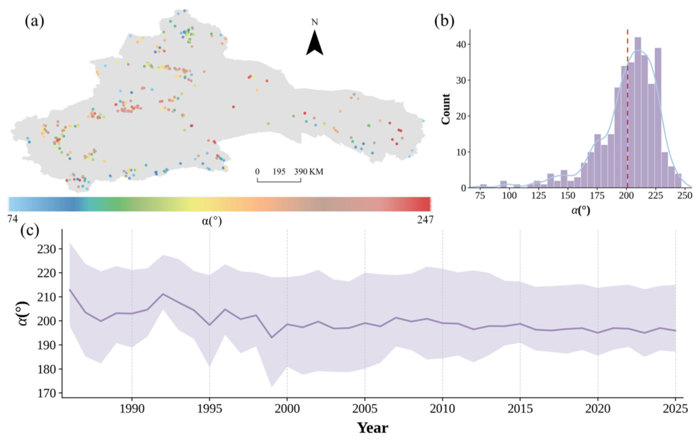
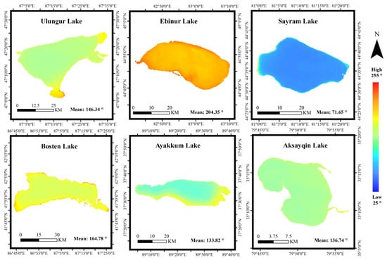
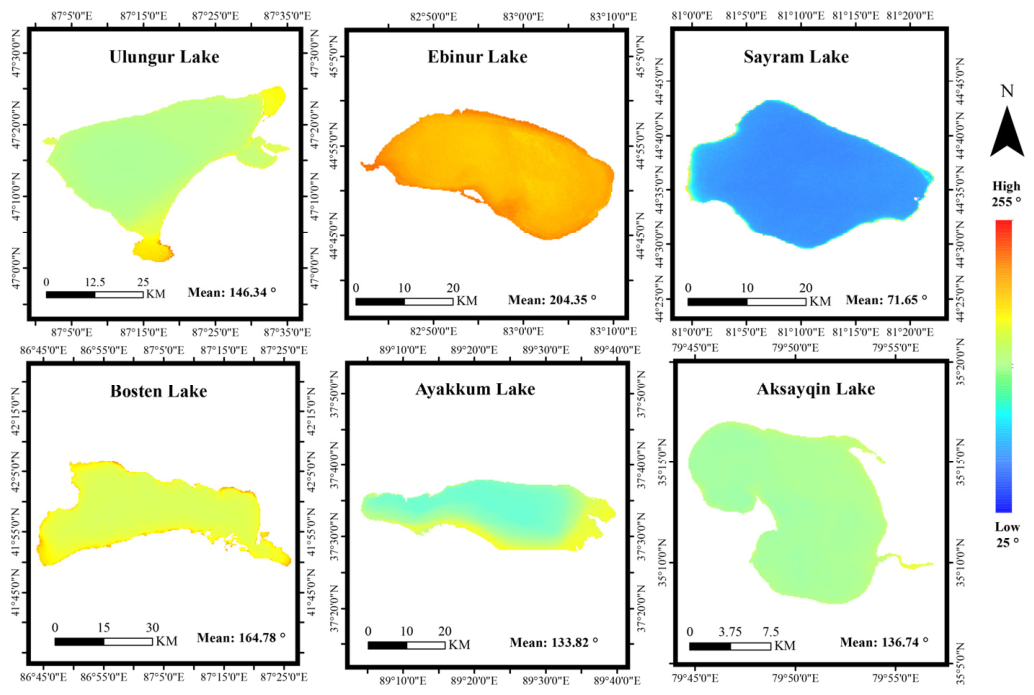
Based on the α calculation formula, lake water color across arid Northwest China was reconstructed for the period 1984–2025 (Figure 2). For each lake, the annual mean α was obtained by averaging all valid water pixels from the March–October observations of that year; the regional annual mean was then calculated as the arithmetic mean of the available lake annual means for that year, and all data used were observed values. The results show that the distribution of α values peaked in the range of approximately 200–230°, with a regional mean of 200.88° (Figure 2b). Strong spatial heterogeneity was observed, with lakes in the central Tianshan Mountains exhibiting generally higher hue angles and the widest α range, where most values exceeded 200°. Several saline lakes along the eastern and southern margins of this region displayed exceptionally high α values (up to 247°), forming distinct local maxima. In contrast, lakes in the southern Kunlun Mountains and northern Altai Mountains generally showed lower α values (Figure 2a). Temporally, the annual mean α exhibited a significant decreasing trend over the study period (slope = −0.261° yr⁻¹, p < 0.001, R² = 0.51), indicating an overall shift in regional lake optical properties during the past four decades (Figure 2c). The water color distributions of six representative lakes further revealed pronounced spatial differences at both inter- and intra-lake scales (Figure 3). Among these lakes, Sayram Lake exhibited the lowest overall α values (mean = 71.65°), whereas Bosten, Ulungur, Ayakkum, and Aksayqin lakes showed intermediate values. Ebinur Lake displayed the highest α values (mean = 204.35°), likely associated with its shallow water depth and elevated suspended sediment concentrations. Within individual lakes, a consistent spatial gradient was observed, characterized by lower α values in central deep-water regions and increasing values toward shallow nearshore zones, with additional localized patches of anomalously high or low values. Collectively, these findings demonstrate that lake water color in arid Northwest China is strongly regulated by geographic settings at the regional scale while exhibiting substantial spatial heterogeneity controlled by local lake morphology and optical conditions.

Figure 2. (a) Spatial distribution of mean hue angle from 1984 to 2025. (b) Statistics of the mean hue angle from 1984 to 2025 (the curve is the kernel density estimation line, and the dashed line is the mean α). (c) Annual average trend of α, with the purple band representing the quartile range and the curve representing the mean.

Figure 3. Spatial distribution of α in six typical lakes.

3.2. Lake Water Color Phenology Distribution and Its Stability

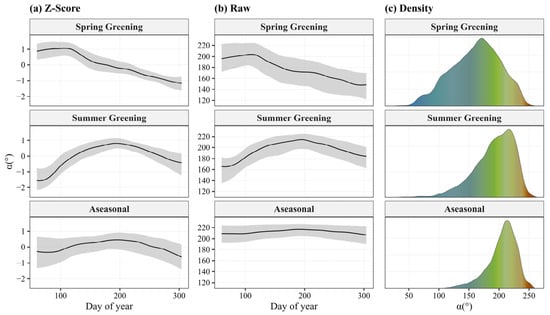
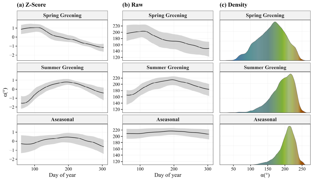
Based on seasonal variation data across seven periods, a subset of seasonal curves was first classified as Aseasonal using an optimization-based threshold, after which clustering analysis of the remaining curves effectively distinguished two distinct phenological modes: Spring Greening and Summer Greening (Figure 4). High mean Jaccard similarity indices derived from bootstrap sampling (0.934 and 0.923, respectively) confirm the robustness and consistency of these clusters, indicating stable lake assignments across repeated resampling iterations. Specifically, the Spring Greening pattern (n = 243, 11.3%) exhibits peak greenness in spring followed by a shift toward blue, displaying a unimodal, positively skewed distribution in which the hue angle declines progressively over the growing season. Compared with Aseasonal lakes, this cluster has a significantly greener median hue angle (median α = 170.74°, p < 0.0001) and the highest seasonal variability (mean SD = 24.93°). Summer Greening lakes (n = 296, 13.7%) show greening that initiates in spring and peaks in summer, with the hue angle rising and then falling through the growing season and following a positively skewed, unimodal distribution; their mean hue angle (190.75°) is significantly greener than that of Aseasonal lakes (p < 0.0001) and also differs significantly from Spring Greening lakes (p < 0.0001). In contrast, the Aseasonal cluster (n = 1616, 75.0%) displays minimal seasonal variation and the lowest variability (mean SD = 7.67°), with hue angles concentrated around 212°, corresponding to stable high α lakes. The results indicate that lake water-color phenology types in the arid Northwest reflect distinct seasonal timing and magnitude of color variation, while also showing that most lakes retain stable optical signatures, with only a minor proportion undergoing marked and temporally structured seasonal greening.

Figure 4. Lake water color phenology clustering analysis results. (a) Water color phenology displayed in standardized form. (b) Water color phenology displayed in original chromatic angle form (black lines represent medians, gray bands represent the 1st–3rd quartiles for each cluster). (c) α observation value density of various clusters.

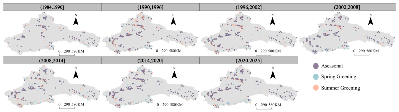
Figure 5 reveals the distribution of lake water-color phenology categories across different periods, indicating clear spatial and temporal variations in these patterns within the arid region of Northwest China. Over time, the proportions of the phenological categories fluctuated notably across decades, with peak occurrences shifting among different periods. Spatially, each category showed distinct geographic aggregation. The Aseasonal lakes were the most widespread, predominantly clustered in the central study region around the Tianshan Mountains, and reached their maximum proportional coverage during the 2015–2020 period (77.8%). Summer Greening lakes, the larger of the two greening modes, were mainly distributed across the mid-latitude belt and peaked in proportion during the 1991–1996 period (22.8%). Spring Greening lakes were comparatively fewer and skewed toward the southern part of the study area, closer to the Kunlun Mountains, peaking during the 2009–2014 period (13.4%). Together, these patterns indicate that the lake water color phenology classification manifests a regionally stable spatial configuration, which may reflect the influence of underlying physiographic and climatic gradients, alongside continuous internal dynamics likely driven by decadal-scale environmental changes evidenced by the maintenance of relatively fixed spatial aggregation zones for distinct phenological types concurrent with significant variations in their relative proportions over time.

Figure 5. Distribution of lake water color phenology categories in different periods.

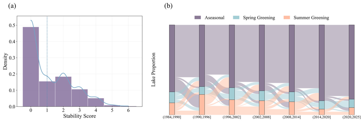
Lake color phenological stability was characterized by the frequency of transitions between categories over the study period. Lakes with no transitions were the most common (n = 170), whereas those with six transitions were the rarest (n = 1) (Figure 6a). Among all lakes, 48.4% remained within a single phenological category, 39.8% occupied two categories, and 11.7% experienced all three categories, revealing substantial heterogeneity in phenological stability across lakes in arid Northwest China. Notably, among lakes that never transitioned, the Aseasonal lakes exhibited significantly higher stability than Summer Greening lakes (p < 0.01), whereas the difference from Spring Greening lakes was not significant, and no significant difference was detected between the two seasonal types. Across the seven periods, Aseasonal lakes consistently maintained the highest stability, with self-retention rates exceeding 80% in most periods and an approximately 89% probability of remaining in the same cluster across consecutive intervals. In contrast, seasonal lakes showed markedly lower stability, with mean self-retention rates of 54.1% for Spring Greening and 43.8% for Summer Greening lakes. When transitions did occur, both seasonal types were more likely to shift toward Aseasonal states (27.7% and 45.4%, respectively), further underscoring the directional nature of phenological change and the stabilizing role of Aseasonal conditions in this arid region (Figure 6b). These findings suggest that Aseasonal lakes tend to occupy a more stable position within the phenological dynamics, whereas seasonal lakes appear more prone to transition and show a tendency to shift toward aseasonality over time.

Figure 6. (a) Lake stability score density histogram; a higher score indicates less stability (the solid line represents the kernel density estimation of stability scores, and the dashed line represents the median value). (b) Sankey diagram showing the distribution of lake water color phenology changes in different periods.

3.3. Characteristics of Lake Water Color Resilience

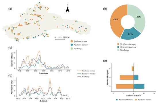
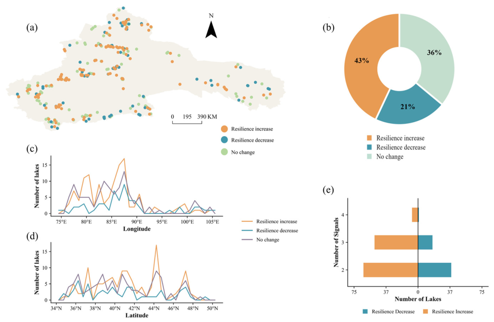
Using detrended hue angle time series, four resilience indicators were evaluated for lakes in the arid region of Northwest China from 1984 to 2025. Among them, approximately 88% of the lakes experienced significant changes in at least two indicators during this period, with 9, 76, and 188 lakes showing significant changes in 4, 3, and 2 indicators, respectively (Figure 7e). Therefore, these lakes possessed sufficient data to assess color resilience based on a comprehensive evaluation principle integrating the four general indicators in the EWS framework. The results show that 43% of the studied lakes in the arid region of Northwest China exhibited increased resilience (Figure 7b), primarily distributed within the region spanning 39–44°N and 80–88°E, with additional occurrences in the northern, central, and western parts of the arid region (Figure 7a–d). In contrast, 21% of the lakes showed declining resilience, exhibiting a relatively clustered distribution mainly within 37–43°N and 83–89°E (Figure 7a–d). Meanwhile, 36% of the lakes showed no significant change in resilience (Figure 7b), with a relatively dispersed distribution across 38–44°N and 80–88°E (Figure 7a–d). Overall, lake color resilience in the arid Northwest exhibits pronounced spatial heterogeneity, with increased resilience as the dominant trajectory, while lakes with declining resilience show distinct geographical clustering, indicating that resilience change is not randomly distributed but is associated with specific environmental contexts.

Figure 7. (a) Spatial distribution of lake water-color resilience changes. (b) Statistics of lakes by resilience change type. (c) Variation in the number of lakes for different water-color resilience types with longitude. (d) Variation in the number of lakes for different water-color resilience types with latitude. (e) The number of lakes exhibiting varying numbers of resilience change signals.

4. Discussion

4.1. Driver Analysis of Lake Water Color Dynamics

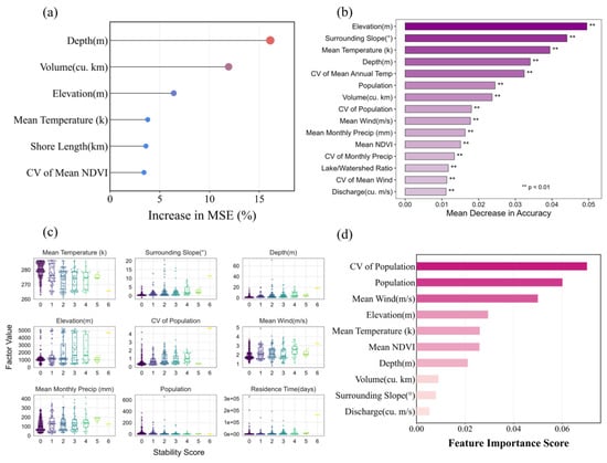
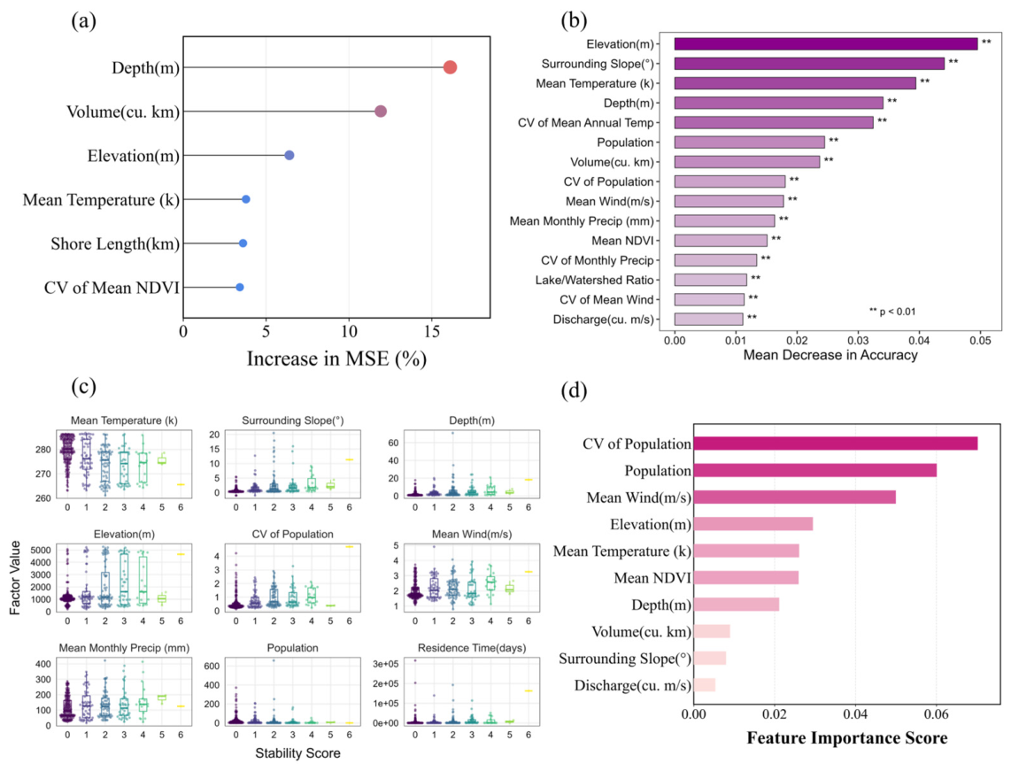
Driver analysis revealed distinct hierarchical associations with lake water color dynamics (Figure 8). Water color (α, R² = 0.54) was most strongly associated with lake morphology, with depth and lake volume showing the highest importance, followed by elevation (Figure 8a). These morphological characteristics regulate light penetration, thermal stratification, water residence time, and sediment resuspension, thereby exerting stronger influences on optical properties than climatic or anthropogenic factors [45,72]. Climatic variables, including mean temperature and its interannual variability, together with shoreline length and watershed vegetation variability, may play secondary roles by modulating algal production, dissolved organic matter dynamics, and land–lake exchanges [22,73]. In contrast, lake-color phenology was most strongly associated with watershed topography and thermal conditions (Figure 8b). Elevation and slope were the most important factors, reflecting their regulation of climate, radiation, runoff, and sediment transport processes [74], while mean temperature and its interannual variability governed seasonal biological dynamics, particularly algal growth cycles [73,75]. Lake depth, morphology, and human activities showed secondary associations with phenological patterns. Lake stability was associated with a combination of lake morphology, climate, and human activities (Figure 8c). Depth, surrounding slope, residence time, temperature, elevation, and wind speed were the factors most associated with stability; high-elevation, cold, and windy lakes tended to be less stable, consistent with disturbances in thermal structure, mixing, and nutrient dynamics reported previously [1,72]. Human-activity variables showed contrasting associations: higher mean watershed population was associated with greater stability, whereas greater interannual population variability was associated with lower stability, suggesting that the temporal consistency of human activity, rather than its magnitude alone, co-varies with lake stability [76]. Lake water color resilience exhibited a markedly different pattern, being most strongly associated with anthropogenic factors rather than natural lake characteristics (Figure 8d). The interannual variability of watershed population was the most important factor, followed by population size and mean wind speed, emphasizing the importance of sustained rather than fluctuating human pressure for maintaining resilience [67,76,77]. Climatic and topographic variables, including elevation and temperature, were secondary predictors, potentially linked to regional climate and meltwater supply [16,69,78], while wind-driven mixing [72] and watershed vegetation dynamics [41] further influenced resilience. Overall, the four response variables exhibited a clear hierarchical pattern of associations: lake morphology was most strongly associated with water color, topography with water-color phenology, stability with the combined associations of morphology, climate, and human activities, whereas lake water color resilience was chiefly associated with the temporal dynamics of anthropogenic pressure.

Figure 8. Importance of lake-attribute, climatic, landscape, and anthropogenic drivers for (a) lake water color (evaluated by MSE increase), (b) water color phenology (evaluated by mean decrease in accuracy), (c) water color phenology stability (boxplots of the significant factors grouped by stability score), and (d) water color resilience change.

4.2. Response Relationship Between Lake Water Color and Water Quality Parameters and Its Optical Mechanism Analysis

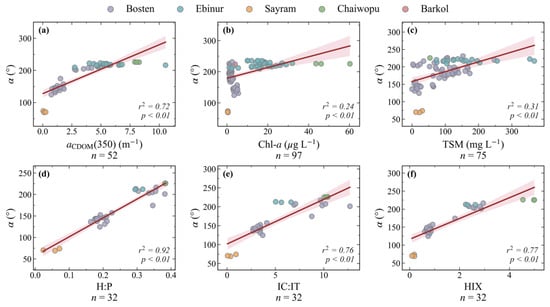
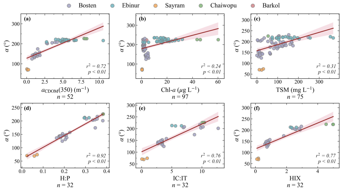
The hue angle (α) was significantly positively related to the major optically active constituents (Figure 9, p < 0.01), with the strongest relationship observed for aCDOM(350) (R² = 0.72), followed by TSM (R² = 0.31) and Chl-a (R² = 0.24). These relationships reflect the combined effects of CDOM absorption in the UV-blue region, phytoplankton pigment absorption, and suspended-particle scattering on water-leaving reflectance, which collectively drive variations in α [29,79]. More importantly, α exhibited stronger positive relationships with the DOM fluorescence indices H:P (R² = 0.92), IC:IT (R² = 0.76), and HIX (R² = 0.77) [80,81]. These indices collectively reflect the relative contribution of humic-like versus protein-like DOM and the degree of humification [80,82]. Their positive relationships with α indicate that increasing humic-like DOM is associated with larger hue angles and a shift in water color toward longer wavelengths. Because humic-like DOM is generally associated with terrestrial inputs, whereas protein-like DOM is more closely linked to autochthonous production, these relationships further suggest that increasing α may reflect a greater terrestrial contribution to DOM [33]. However, these are pooled relationships. Because α is strongly clustered by lake, the pooled fits are driven largely by contrasts among these optically distinct lakes rather than by variation within them, and within individual lakes the associations are weaker and lake-dependent. We therefore interpret α as a robust integrator of among-lake DOM and humification contrasts rather than a validated quantitative water-quality proxy for individual lakes.

Figure 9. Scatter plots showing the quantitative relationships between the hue angle (α) and various in situ water-quality parameters. (a) aCDOM(350); (b) Chl-a; (c) TSM; (d) H:P; (e) IC:IT; (f) HIX. The solid red lines represent the linear regression fits, and the pink shaded areas indicate the 95% confidence intervals.

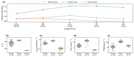
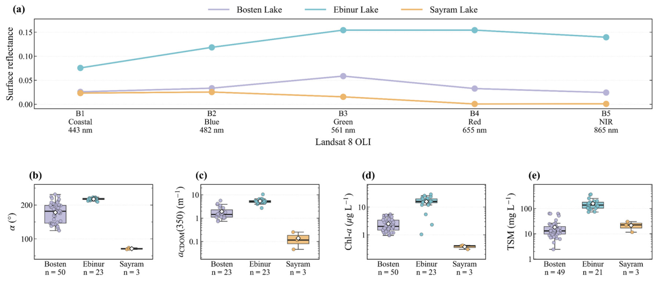
Hue-angle matchups were obtained for all five in situ lakes and used in the regressions above; the per-lake spectral comparison here is restricted to Bosten, Ebinur, and Sayram, whereas Barkol and Chaiwopu each had too few coincident cloud-free samples to characterize their mean spectra reliably. The spectral and water-quality differences among Bosten Lake, Ebinur Lake, and Sayram Lake further illustrate this optical response (Figure 10). Ebinur Lake exhibited the highest reflectance across the visible bands, with a broad maximum in the green-red region, whereas Bosten Lake showed intermediate reflectance with a more pronounced green-band peak. In contrast, Sayram Lake had the lowest overall reflectance, particularly in the red and near-infrared bands, consistent with its relatively clear-water optical characteristics [36]. Correspondingly, α differed markedly among the three lakes, with Ebinur Lake showing the highest values, Bosten Lake intermediate values, and Sayram Lake the lowest. Similar inter-lake patterns were evident for a_CDOM(350) and Chl-a, both of which were substantially higher in Ebinur Lake and lowest in Sayram Lake. TSM also differed considerably among the lakes, although its inter-lake pattern did not completely parallel that of α [38,40]. Overall, α is governed by the combined optical effects of absorption and scattering from major optically active constituents, while also responding sensitively to DOM compositional changes. This indicates that hue angle has the potential not only to characterize conventional optical water properties but also to provide insights into organic matter characteristics and source-related variations in heterogeneous arid-region lakes.

Figure 10. Comparison of spectral characteristics and water quality parameters among three representative lakes (Bosten Lake, Ebinur Lake, and Sayram Lake). (a) Landsat 8 OLI-derived remote sensing reflectance spectra for the three lakes. (b–e) Boxplots of the hue angle (α) and various in situ water-quality parameters across the lakes.

4.3. Implications and Limitations for Water Color Monitoring in Arid Regions

The continuous hue angle (α) provides a useful framework for integrating optical variations, ecological dynamics, and environmental responses in arid lake systems. By capturing subtle changes in lake optical states, long-term α trajectories combined with water-color phenology and resilience assessment can improve the detection of ecosystem changes under climatic and anthropogenic pressures [83]. Moreover, the demonstrated relationships between α and both optically active constituents and DOM fluorescence indices suggest that water color has potential not only for characterizing conventional optical properties but also for providing insights into organic matter composition and source-related variations. As an integrated optical indicator, α reflects the combined effects of multiple water constituents, and its potential as a proxy for specific water-quality parameters and for broader lake water-quality assessment can be further strengthened through more extensive field observations and biogeochemical measurements. Future integration of multi-source remote sensing, advanced optical models, and expanded in situ datasets will further enhance the application of hue angle for regional water-quality assessment and ecological monitoring of vulnerable arid-zone lakes.

Several limitations remain in this study. First, at the data level, the long-term reconstruction of water color relies on cross-sensor continuity among TM, ETM+, and OLI, and the radiometric and spectral differences among these sensors may introduce systematic uncertainty. In addition, the 16-day revisit cycle of Landsat, together with cloud cover, results in temporally uneven and missing observations, affecting the fine-scale characterization of water-color change. Moreover, in situ sampling covered only a few representative lakes, which may limit the generality of the relationships between water color and water-quality parameters. Second, at the level of resilience estimation, the early warning signal indicator series computed from sliding windows are serially autocorrelated, which may cause the standard Mann–Kendall test to overestimate the significance of trends. Given the length of our record, it is difficult to fully remove this dependence without a substantial loss of test power. The absolute proportions of the resilience-change categories should therefore be interpreted with caution, whereas their spatial clustering and association with watershed population dynamics remain robust across multiple testing methods and are not affected by this issue. Third, in the driver analysis, collinearity exists among some environmental factors (detailed in Figure S2 of the Supporting Materials), which may to some extent affect the stability of the relative importance ranking of individual factors; therefore, the relevant conclusions should be interpreted in terms of the overall contribution of the factor group. The LandScan population data used to represent human activity have limited spatial resolution and may inadequately represent watershed-scale population dynamics in the sparsely populated arid region; future work should validate this using higher-resolution population data. In addition, longer satellite records and more extensive field sampling will help further reduce these uncertainties.

5. Conclusions

Based on Landsat-derived hue angle data from 1984 to 2025, this study reveals that lake water color across arid Northwest China has undergone a widespread but spatially heterogeneous transformation, characterized by a persistent decline in regional mean hue angle and pronounced geographic contrasts. More importantly, long-term lake-color dynamics were characterized by the dominance of stable Aseasonal phenology, a tendency for seasonal lakes to transition toward aseasonality, and an overall prevalence of increasing water-color resilience, although a smaller proportion of lakes exhibited resilience loss and formed distinct spatial clusters. These changes were associated with a clear hierarchy of environmental factors, with lake morphology most strongly associated with water color, topographic setting with phenological behavior, and the temporal dynamics of watershed population showing the strongest association with resilience. In situ observations further show that hue angle reflects major optically active constituents and DOM composition and sources, highlighting its potential as an extensible proxy for specific water-quality indicators in optically complex arid-zone lakes. Collectively, these findings show that long-term changes in lake water color, phenology, and resilience represent interconnected but differently shaped by different sets of dimensions of lake environmental response, providing a basis for identifying vulnerable lake clusters and improving targeted monitoring and management under growing climatic and anthropogenic pressures.

References

- Adrian, R.; O’Reilly, C.M.; Zagarese, H.; Baines, S.B.; Hessen, D.O.; Keller, W.; Livingstone, D.M.; Sommaruga, R.; Straile, D.; Van Donk, E.; et al. Lakes as sentinels of climate change. Limnol. Oceanogr. 2009, 54, 2283–2297. [Google Scholar] [CrossRef] [Scilit] [PubMed]
- Bennett, E.M.; Carpenter, S.R.; Caraco, N.F. Human Impact on Erodable Phosphorus and Eutrophication: A Global Perspective: Increasing accumulation of phosphorus in soil threatens rivers, lakes, and coastal oceans with eutrophication. BioScience 2001, 51, 227–234. [Google Scholar] [CrossRef] [Scilit]
- Yao, F.; Livneh, B.; Rajagopalan, B.; Wang, J.; Crétaux, J.-F.; Wada, Y.; Berge-Nguyen, M. Satellites reveal widespread decline in global lake water storage. Science 2023, 380, 743–749. [Google Scholar] [CrossRef] [Scilit] [PubMed]
- Xu, N.; Lu, H.; Li, W.; Gong, P. Natural lakes dominate global water storage variability. Sci. Bull. 2024, 69, 1016–1019. [Google Scholar] [CrossRef] [Scilit] [PubMed]
- Heathcote, A.J.; Downing, J.A. Impacts of Eutrophication on Carbon Burial in Freshwater Lakes in an Intensively Agricultural Landscape. Ecosystems 2012, 15, 60–70. [Google Scholar] [CrossRef] [Scilit]
- Liu, D.; Shi, K.; Chen, P.; Yan, N.; Ran, L.; Kutser, T.; Tyler, A.N.; Spyrakos, E.; Woolway, R.I.; Zhang, Y.; et al. Substantial increase of organic carbon storage in Chinese lakes. Nat. Commun. 2024, 15, 8049. [Google Scholar] [CrossRef] [Scilit] [PubMed]
- Jane, S.F.; Hansen, G.J.A.; Kraemer, B.M.; Leavitt, P.R.; Mincer, J.L.; North, R.L.; Pilla, R.M.; Stetler, J.T.; Williamson, C.E.; Woolway, R.I.; et al. Widespread deoxygenation of temperate lakes. Nature 2021, 594, 66–70. [Google Scholar] [CrossRef] [Scilit] [PubMed]
- Huisman, J.; Codd, G.A.; Paerl, H.W.; Ibelings, B.W.; Verspagen, J.M.H.; Visser, P.M. Cyanobacterial blooms. Nat. Rev. Microbiol. 2018, 16, 471–483. [Google Scholar] [CrossRef] [Scilit] [PubMed]
- Feng, L.; Wang, Y.; Hou, X.; Qin, B.; Kutser, T.; Qu, F.; Chen, N.; Paerl, H.W.; Zheng, C. Harmful algal blooms in inland waters. Nat. Rev. Earth Environ. 2024, 5, 631–644. [Google Scholar] [CrossRef] [Scilit] [PubMed]
- Knoll, L.B.; Williamson, C.E.; Pilla, R.M.; Leach, T.H.; Brentrup, J.A.; Fisher, T.J. Browning-related oxygen depletion in an oligotrophic lake. Inland Waters 2018, 8, 255–263. [Google Scholar] [CrossRef] [Scilit]
- Müller, B.; Bryant, L.; Matzinger, A.; Wuest, A. Hypolimnetic Oxygen Depletion in Eutrophic Lakes. Environ. Sci. Technol. 2012, 46, 9964–9971. [Google Scholar] [CrossRef] [Scilit] [PubMed]
- Yang, J.-M.; Ma, L.-G.; Li, C.-Z.; Liu, Y.; Ding, J.-L.; Yang, S.-T. Temporal-spatial variations and influencing factors of Lakes in inland arid areas from 2000 to 2017: A case study in Xinjiang. Geomat. Nat. Hazards Risk 2019, 10, 519–543. [Google Scholar] [CrossRef] [Scilit]
- Li, X.; Yao, X.; Sun, M.; Gong, P.; An, L.; Qi, M.; Gao, Y. Spatial-temporal variations in lakes in northwest China from 2000 to 2014. Acta Ecol. Sin. 2018, 38, 96–104. [Google Scholar] [CrossRef] [Scilit]
- Wang, N.-A.; Zhao, Q.; Hu, G.; Chen, Y.-S. Climatic and humanistic background of desertification process in the recent 2000 years in Hexi Corridor, China. J. Desert Res. 2003, 23, 95. [Google Scholar]
- Xu, N.; Li, W.; Gong, P.; Lu, H. Satellite altimeter observed surface water increase across lake-rich regions of the Arctic. Innovation 2024, 5, 100714. [Google Scholar] [CrossRef] [Scilit] [PubMed]
- Zhu, Y.; Chen, Y.; Ren, L.; Lü, H.; Zhao, W.; Yuan, F.; Xu, M. Ecosystem restoration and conservation in the arid inland river basins of Northwest China: Problems and strategies. Ecol. Eng. 2016, 94, 629–637. [Google Scholar] [CrossRef] [Scilit]
- Zhang, W.; Wang, S.; Zhang, B.; Zhang, F.; Shen, Q.; Wu, Y.; Mei, Y.; Qiu, R.; Li, J. Analysis of the water color transitional change in Qinghai Lake during the past 35 years observed from Landsat and MODIS. J. Hydrol. Reg. Stud. 2022, 42, 101154. [Google Scholar] [CrossRef] [Scilit]
- Cao, Z.; Melack, J.M.; Liu, M.; Kutser, T.; Duan, H.; Ma, R. Shifts, Trends, and Drivers of Lake Color Across China Since the 1980s. Geophys. Res. Lett. 2023, 50, e2023GL103225. [Google Scholar] [CrossRef] [Scilit]
- Ying, H.; Wang, S.; Zhang, B.; Mao, Z.; Zhang, F.; Li, J. Earth observation reveals the shifting patterns of China’s lake colour driven by climate change and land cover. J. Environ. Manag. 2024, 370, 122809. [Google Scholar] [CrossRef] [Scilit] [PubMed]
- Chen, Q.; Li, Z.; Jin, Z.; Yao, S.; Zhou, Y.; Wu, H.; Liu, Y.; Zhang, G.; Liu, Y.; Yang, X.; et al. Evolution patterns, driving mechanisms, and ecological indicative effects of 730 lakes water color in the Yangtze River Basin (1984–2023). J. Hydrol. 2025, 653, 132695. [Google Scholar] [CrossRef] [Scilit]
- Li, L.; Ning, Y.; Cao, Z.; Xue, K.; Song, C. A national-scale assessment on the spatial and temporal variations in water color for urban lakes in China. Sci. Total Environ. 2024, 945, 173951. [Google Scholar] [CrossRef] [Scilit] [PubMed]
- Huan, S.; Xiao, C.; Feng, Z. Unravelling mystery of lake color changes on the Tibetan Plateau: From mechanisms to prediction. Ecol. Indic. 2025, 178, 113936. [Google Scholar] [CrossRef] [Scilit]
- Topp, S.N.; Pavelsky, T.M.; Dugan, H.A.; Yang, X.; Gardner, J.; Ross, M.R.V. Shifting Patterns of Summer Lake Color Phenology in Over 26,000 US Lakes. Water Resour. Res. 2021, 57, e2020WR029123. [Google Scholar] [CrossRef] [Scilit] [PubMed]
- Xue, K.; Ma, R.; Hu, M.; Li, Y. Anthropogenic and climatic factors regulate algal bloom intensity and timing in global lakes under climate change. Commun. Earth Environ. 2026, 7, 458. [Google Scholar] [CrossRef] [Scilit]
- Han, Y.; Lin, Q.; Huang, S.; Du, C.; Shen, J.; Zhang, K. Human Impacts Dominate Global Loss of Lake Ecosystem Resilience. Geophys. Res. Lett. 2024, 51, e2024GL109298. [Google Scholar] [CrossRef] [Scilit]
- Xiong, S.; Yang, F. Ecological resilience in water-land transition zones: A case study of the Dongting Lake region, China. Ecol. Indic. 2024, 166, 112284. [Google Scholar] [CrossRef] [Scilit]
- Pourmoghim, P.; Behboudian, M.; Kerachian, R. An uncertainty-based framework for evaluating and improving the long-term resilience of lakes under anthropogenic droughts. J. Environ. Manag. 2022, 301, 113900. [Google Scholar] [CrossRef] [Scilit] [PubMed]
- Zhang, K.; Dong, X.; Yang, X.; Kattel, G.; Zhao, Y.; Wang, R. Ecological shift and resilience in China’s lake systems during the last two centuries. Glob. Planet. Change 2018, 165, 147–159. [Google Scholar] [CrossRef] [Scilit]
- Pitarch, J.; van der Woerd, H.J.; Brewin, R.J.W.; Zielinski, O. Optical properties of Forel-Ule water types deduced from 15 years of global satellite ocean color observations. Remote Sens. Environ. 2019, 231, 111249. [Google Scholar] [CrossRef] [Scilit]
- Van der Woerd, H.J.; Wernand, M.R. Hue-Angle Product for Low to Medium Spatial Resolution Optical Satellite Sensors. Remote Sens. 2018, 10, 180. [Google Scholar] [CrossRef] [Scilit]
- Wernand, M.R.; Hommersom, A.; van der Woerd, H.J. MERIS-based ocean colour classification with the discrete Forel–Ule scale. Ocean Sci. 2013, 9, 477–487. [Google Scholar] [CrossRef] [Scilit]
- Ye, M.; Sun, Y. Review of the Forel–Ule Index based on in situ and remote sensing methods and application in water quality assessment. Environ. Sci. Pollut. Res. 2022, 29, 13024–13041. [Google Scholar] [CrossRef] [Scilit] [PubMed]
- Zhao, Z.; Shi, K.; Zhang, Y.; Zhou, Y.; Qin, B. Increased dominance of terrestrial component in dissolved organic matter in Chinese lakes. Water Res. 2024, 249, 121019. [Google Scholar] [CrossRef] [Scilit] [PubMed]
- Jiang, Q.; Sun, Y.; Jeppesen, E.; Smol, J.P.; Scavia, D.; Hecky, R.E.; Mehner, T.; Qin, Y.; Tong, Y.; Qin, B.; et al. Persistent inequities in global lake science. Nat. Rev. Earth Environ. 2025, 6, 629–631. [Google Scholar] [CrossRef] [Scilit]
- Shen, X.; Ke, C.-Q.; Duan, Z.; Cai, Y.; Li, H.; Xiao, Y. Satellite Observations Reveal Widespread Color Variations in Global Lakes Since the 1980s. Water Resour. Res. 2025, 61, e2023WR036926. [Google Scholar] [CrossRef] [Scilit]
- Wang, S.; Li, J.; Zhang, B.; Lee, Z.; Spyrakos, E.; Feng, L.; Liu, C.; Zhao, H.; Wu, Y.; Zhu, L.; et al. Changes of water clarity in large lakes and reservoirs across China observed from long-term MODIS. Remote Sens. Environ. 2020, 247, 111949. [Google Scholar] [CrossRef] [Scilit]
- He, Y.; Woolway, R.I.; Shi, K.; Yang, X. Widespread brightening of the underwater light environment across China’s lakes. Commun. Earth Environ. 2026, 7, 492. [Google Scholar] [CrossRef] [Scilit]
- Li, M.; Sun, Y.; Li, X.; Cui, M.; Huang, C. An Improved Eutrophication Assessment Algorithm of Estuaries and Coastal Waters in Liaodong Bay. Remote Sens. 2021, 13, 3867. [Google Scholar] [CrossRef] [Scilit]
- Deng, M.; Ma, R.; Wang, L.; Hu, M.; Xue, K.; Cao, Z.; Xiong, J.; Yu, Z. A non-optically active lake salinity dataset by satellite remote sensing. Sci. Data 2025, 12, 1324. [Google Scholar] [CrossRef] [Scilit] [PubMed]
- Yang, X.; Tong, R.; Ma, L.; Li, J.; Wang, S.; Tian, L. Monitoring water color anomaly of lakes based on an integrated method using Landsat-8 OLI images. Int. J. Digit. Earth 2022, 15, 1567–1587. [Google Scholar] [CrossRef] [Scilit]
- Zhan, Y.; Ma, C.; Yan, Y.; Zhu, J.; Ji, Y.; Ma, C.; Luo, Y. Spatial differentiation characteristics of vegetation greening rates and climate attribution in China’s arid and semi-arid regions. Glob. Ecol. Conserv. 2023, 46, e02563. [Google Scholar] [CrossRef] [Scilit]
- Wang, H.; Chen, Y.; Xun, S.; Lai, D.; Fan, Y.; Li, Z. Changes in daily climate extremes in the arid area of northwestern China. Theor. Appl. Climatol. 2013, 112, 15–28. [Google Scholar] [CrossRef] [Scilit]
- Ding, H.; Hao, X. Spatiotemporal change and drivers analysis of desertification in the arid region of northwest China based on geographic detector. Environ. Chall. 2021, 4, 100082. [Google Scholar] [CrossRef] [Scilit]
- Crawford, C.J.; Roy, D.P.; Arab, S.; Barnes, C.; Vermote, E.; Hulley, G.; Gerace, A.; Choate, M.; Engebretson, C.; Micijevic, E.; et al. The 50-year Landsat collection 2 archive. Sci. Remote Sens. 2023, 8, 100103. [Google Scholar] [CrossRef] [Scilit]
- Messager, M.L.; Lehner, B.; Grill, G.; Nedeva, I.; Schmitt, O. Estimating the volume and age of water stored in global lakes using a geo-statistical approach. Nat. Commun. 2016, 7, 13603. [Google Scholar] [CrossRef] [Scilit] [PubMed]
- Peng, S.; Ding, Y.; Liu, W.; Li, Z. 1 km monthly temperature and precipitation dataset for China from 1901 to 2017. Earth Syst. Sci. Data 2019, 11, 1931–1946. [Google Scholar] [CrossRef] [Scilit]
- Pitarch, J.; Bellacicco, M.; Marullo, S.; Van Der Woerd, H.J. Global maps of Forel–Ule index, hue angle and Secchi disk depth derived from 21 years of monthly ESA Ocean Colour Climate Change Initiative data. Earth Syst. Sci. Data 2021, 13, 481–490. [Google Scholar] [CrossRef] [Scilit]
- Bukata, R.P.; Pozdnyakov, D.V.; Jerome, J.H.; Tanis, F.J. Validation of a radiometric color model applicable to optically complex water bodies. Remote Sens. Environ. 2001, 77, 165–172. [Google Scholar] [CrossRef] [Scilit]
- Wang, S.; Li, J.; Zhang, B.; Spyrakos, E.; Tyler, A.N.; Shen, Q.; Zhang, F.; Kuster, T.; Lehmann, M.K.; Wu, Y.; et al. Trophic state assessment of global inland waters using a MODIS-derived Forel-Ule index. Remote Sens. Environ. 2018, 217, 444–460. [Google Scholar] [CrossRef] [Scilit]
- Feng, S.; Zhang, N.; Shen, J. Method of cloud detection with hyperspectral remote sensing image based on the reflective characteristics. Chin. Opt. 2015, 8, 198–204. [Google Scholar] [CrossRef] [Scilit]
- Tan, Z.; Wang, S.; Li, J.; Zhang, F.; Zhang, B. Consistency correction of multi-source satellite-derived lake water color indices: A case study of typical lakes on the Tibetan Plateau. Natl. Remote Sens. Bull. 2025, 29, 3626–3639. [Google Scholar] [CrossRef] [Scilit]
- Wang, S.; Li, J.; Zhang, W.; Cao, C.; Zhang, F.; Shen, Q.; Zhang, X.; Zhang, B. A dataset of remote-sensed Forel-Ule Index for global inland waters during 2000–2018. Sci. Data 2021, 8, 26. [Google Scholar] [CrossRef] [Scilit] [PubMed]
- Nadaraya, E.A. On estimating regression. Theory Probab. Its Appl. 1964, 9, 141–142. [Google Scholar] [CrossRef] [Scilit] [PubMed]
- Watson, G.S. Smooth Regression Analysis. Sankhyā Indian J. Stat. Ser. A 1964, 26, 359–372. [Google Scholar]
- Byrnes, D.K.; Van Meter, K.J.; Basu, N.B. Long-Term Shifts in U.S. Nitrogen Sources and Sinks Revealed by the New TREND-Nitrogen Data Set (1930–2017). Glob. Biogeochem. Cycles 2020, 34, e2020GB006626. [Google Scholar] [CrossRef] [Scilit]
- Savoy, P.; Appling, A.P.; Heffernan, J.B.; Stets, E.G.; Read, J.S.; Harvey, J.W.; Bernhardt, E.S. Metabolic rhythms in flowing waters: An approach for classifying river productivity regimes. Limnol. Oceanogr. 2019, 64, 1835–1851. [Google Scholar] [CrossRef] [Scilit]
- Sakoe, H.; Chiba, S. Dynamic programming algorithm optimization for spoken word recognition. IEEE Trans. Acoust. Speech Signal Process. 1978, 26, 43–49. [Google Scholar] [CrossRef] [Scilit]
- Hollander, M.; Wolfe, D.A.; Chicken, E. Nonparametric Statistical Methods, 3rd ed.; John Wiley & Sons: Hoboken, NJ, USA, 2015. [Google Scholar]
- Dunn, O.J. Multiple comparisons among means. J. Am. Stat. Assoc. 1961, 56, 52–64. [Google Scholar] [CrossRef]
- Bonferroni, C. Teoria statistica delle classi e calcolo delle probabilita. Pubbl. R Ist. Super. Sci. Econ. Commer. Firenze 1936, 8, 3–62. [Google Scholar]
- Krumbein, W.C.; Dacey, M.F. Markov chains and embedded Markov chains in geology. J. Int. Assoc. Math. Geol. 1969, 1, 79–96. [Google Scholar] [CrossRef] [Scilit]
- Scheffer, M.; Carpenter, S.; Dakos, V.; Nes, E. Generic Indicators of Ecological Resilience: Inferring the Chance of a Critical Transition. Annu. Rev. Ecol. Evol. Syst. 2015, 46, 145–167. [Google Scholar] [CrossRef] [Scilit]
- Dakos, V.; Carpenter, S.; Nes, E.; Scheffer, M. Resilience indicators: Prospects and limitations of early warnings of regime shifts. Philos. Trans. R. Soc. B Biol. Sci. 2015, 370, 20130263. [Google Scholar] [CrossRef] [Scilit]
- Gsell, A.S.; Scharfenberger, U.; Özkundakci, D.; Walters, A.; Hansson, L.-A.; Janssen, A.B.G.; Nõges, P.; Reid, P.C.; Schindler, D.E.; Van Donk, E.; et al. Evaluating early-warning indicators of critical transitions in natural aquatic ecosystems. Proc. Natl. Acad. Sci. USA 2016, 113, E8089–E8095. [Google Scholar] [CrossRef] [Scilit] [PubMed]
- Smith, T.; Traxl, D.; Boers, N. Empirical evidence for recent global shifts in vegetation resilience. Nat. Clim. Change 2022, 12, 477–484. [Google Scholar] [CrossRef] [Scilit]
- Feng, Y.; Su, H.; Tang, Z.; Wang, S.; Zhao, X.; Zhang, H.; Ji, C.; Zhu, J.; Xie, P.; Fang, J. Reduced resilience of terrestrial ecosystems locally is not reflected on a global scale. Commun. Earth Environ. 2021, 2, 88. [Google Scholar] [CrossRef] [Scilit]
- Rocha, J.C. Ecosystems are showing symptoms of resilience loss. Environ. Res. Lett. 2022, 17, 065013. [Google Scholar] [CrossRef] [Scilit]
- Kendall, M.G. Rank Correlation Methods; Charles Griffin: London, UK, 1948. [Google Scholar]
- Huang, R.; Xu, L.; Liu, J. Research on spatio-temporal change of temperature in the Northwest Arid Area. Shengtai Xuebao/Acta Ecol. Sin. 2013, 33, 4078–4089. [Google Scholar] [CrossRef] [Scilit]
- Tomczak, M.; Tomczak-Łukaszewska, E. The need to report effect size estimates revisited. An overview of some recommended measures of effect size. Trends Sport Sci. 2014, 21, 19–25. [Google Scholar]
- Cohen, J. Statistical Power Analysis for the Behavioral Sciences; Lawrence Erlbaum Associates: Hillsdale, NJ, USA, 1988. [Google Scholar]
- Qin, Z.; Lai, Y.; Tian, Y. Study on failure mechanism of a plain irrigation reservoir soil bank slope under wind wave erosion. Nat. Hazards 2021, 109, 567–592. [Google Scholar] [CrossRef] [Scilit]
- Priscu, J.C.; Goldman, C.R. The effect of temperature on photosynthetic and respiratory electron transport system activity in the shallow and deep-living phytoplankton of a subalpine lake. Freshw. Biol. 1984, 14, 143–155. [Google Scholar] [CrossRef] [Scilit]
- Catalan, J.; Camarero, L.; Felip, M.; Pla, S.; Ventura, M.; Buchaca, T.; Bartumeus, F.; Mendoza, G.d.; Miró, A. High mountain lakes: Extreme habitats and witnesses of environmental changes. Limnetica 2006, 25, 551–584. [Google Scholar] [CrossRef] [Scilit]
- Wang, C.; Wang, M.; Xie, M.; Qi, L.; Chen, M.; Song, X.; Zhou, Z.; Shi, X.; Yin, J.; Wei, Y.a.; et al. Climate extremes intensify global lake eutrophication by increasing the stress resistance of harmful bloom-forming algae. Nat. Commun. 2026, 17, 2859. [Google Scholar] [CrossRef] [Scilit] [PubMed]
- Grant, L.; Vanderkelen, I.; Gudmundsson, L.; Tan, Z.; Perroud, M.; Stepanenko, V.M.; Debolskiy, A.V.; Droppers, B.; Janssen, A.B.G.; Woolway, R.I.; et al. Attribution of global lake systems change to anthropogenic forcing. Nat. Geosci. 2021, 14, 849–854. [Google Scholar] [CrossRef] [Scilit]
- Han, Y.; Zhang, K.; Lin, Q.; Huang, S.; Yang, X. Assessing lake ecosystem health from disturbed anthropogenic landscapes: Spatial patterns and driving mechanisms. Ecol. Indic. 2023, 147, 110007. [Google Scholar] [CrossRef] [Scilit]
- Woolway, R.I.; Kraemer, B.M.; Lenters, J.D.; Merchant, C.J.; O’Reilly, C.M.; Sharma, S. Global lake responses to climate change. Nat. Rev. Earth Environ. 2020, 1, 388–403. [Google Scholar] [CrossRef] [Scilit]
- Zhang, Y.; Zhou, L.; Zhou, Y.; Zhang, L.; Yao, X.; Shi, K.; Jeppesen, E.; Yu, Q.; Zhu, W. Chromophoric dissolved organic matter in inland waters: Present knowledge and future challenges. Sci. Total Environ. 2021, 759, 143550. [Google Scholar] [CrossRef] [Scilit] [PubMed]
- Zhou, Y.; Shi, K.; Zhang, Y.; Jeppesen, E.; Liu, X.; Zhou, Q.; Wu, H.; Tang, X.; Zhu, G. Fluorescence peak integration ratio IC:IT as a new potential indicator tracing the compositional changes in chromophoric dissolved organic matter. Sci. Total Environ. 2017, 574, 1588–1598. [Google Scholar] [CrossRef] [Scilit] [PubMed]
- Zsolnay, A.; Baigar, E.; Jimenez, M.; Steinweg, B.; Saccomandi, F. Differentiating with fluorescence spectroscopy the sources of dissolved organic matter in soils subjected to drying. Chemosphere 1999, 38, 45–50. [Google Scholar] [CrossRef] [Scilit] [PubMed]
- Cai, X.; Lei, S.; Li, Y.; Li, J.; Xu, J.; Lyu, H.; Li, J.; Dong, X.; Wang, G.; Zeng, S. Humification levels of dissolved organic matter in the eastern plain lakes of China based on long-term satellite observations. Water Res. 2024, 250, 120991. [Google Scholar] [CrossRef] [Scilit] [PubMed]
- Woolway, R.I.; Zhang, Y.; Jennings, E.; Zohary, T.; Jane, S.F.; Jansen, J.; Weyhenmeyer, G.A.; Long, D.; Fleischmann, A.; Feng, L.; et al. Extreme and compound events in lakes. Nat. Rev. Earth Environ. 2025, 6, 593–611. [Google Scholar] [CrossRef] [Scilit]
Disclaimer/Publisher’s Note: The statements, opinions and data contained in all publications are solely those of the individual author(s) and contributor(s) and not of MDPI and/or the editor(s). MDPI and/or the editor(s) disclaim responsibility for any injury to people or property resulting from any ideas, methods, instructions or products referred to in the content. |
© 2026 by the authors. Licensee MDPI, Basel, Switzerland. This article is an open access article distributed under the terms and conditions of the Creative Commons Attribution (CC BY) license.