


Highlights
What are the main findings?
- A cross-resolution fusion network is developed that couples 10 m resolution AlphaEarth Foundations embeddings with 2 m resolution GF-1 imagery for litchi orchard extraction;
- Semantic anchors carry the coarse target semantics while GF-1 decides the spatial confidence region, and a reliability-gated head performs selective refinement, operating exclusively on uncertain regions.
What is the implication of the main finding?
- Extends the usable resolution of geospatial foundation-model embeddings from landcover mapping to parcel-level orchard delineation;
- Achieves the highest IoU and F1 among eight comparison networks and yields a wallto- wall 2 m litchi map of Shenzhen.
Abstract
Litchi is an important cash crop in China. Accurate litchi orchard extraction is crucial for agricultural management and economic development. However, litchi orchards are spectrally very similar to evergreen broad-leaved forests and are poorly resolved in medium- and low-resolution satellite imagery, so large-scale extraction remains challenging. A cross-resolution fusion network via semantic anchor-graph enhancement (SAGE-Net) is therefore proposed, using a dual-branch encoder–decoder to aggregate complementary features of AlphaEarth Foundations (AEF) embeddings and GF-1 imagery. To enable semantic interaction across resolutions, the SAGE module is designed to gather the AEF embeddings into a few semantic anchors, reason over the anchor graph, and scatter them back under GF-1 guidance, so that semantic content and spatial extent are supplied by the source better suited to each. To refine the coarse prediction to full resolution without discarding what is already reliable, the reliability-adaptive correction (RAC) head is designed to gate a detail-guided correction by the confidence and local consistency of that prediction, concentrating refinement where it is uncertain. In Shenzhen, SAGE-Net attains the highest IoU (0.5660) and F1-score (0.7229) among eight comparison methods, with a Precision of 0.7162 and a Recall of 0.7297. Under stricter protocols that separate the training and the evaluation patches by a 256 m buffer or by whole spatial blocks, the IoU falls to 0.5224 and 0.5000 and SAGE-Net remains the most accurate of the networks retested, by a smaller margin. The results demonstrate the value of role-aware enhancement and reliability-adaptive correction for fine-grained orchard mapping, and confirm AEF embeddings as an effective supplementary data source for large-scale mapping.
1. Introduction
Litchi (Litchi chinensis) is an important subtropical fruit cash crop in China, its national production accounts for about 90% of the global total production [1]. By 2024, the total area of litchi plantations in China had grown to over 5234.2 km2 [2]. Accurate litchi orchard extraction is of great significance for agricultural management, litchi industry structure adjustment, and economic development [3]. Currently, litchi extraction is mostly concentrated in the field of unmanned aerial vehicle (UAV) remote sensing, which is only applicable to a local area and not conducive to regional and national monitoring [4,5]. Satellite remote sensing provides an effective means for large-scale extraction. However, the inherent trade-off between spectral and spatial resolution in optical imaging systems presents a significant obstacle to the accurate extraction of litchi orchards, i.e., it is difficult to achieve both high spatial resolution and high spectral resolution at the same time [6]. Consequently, large-scale litchi extraction faces huge challenges: (1) litchi is mainly distributed in the lush vegetation areas, which makes it difficult to distinguish from evergreen broad-leaved forests in terms of the spectrum within a limited spectral band, (2) litchi orchards show poor textural visibility in medium- and low-resolution satellite imagery and are easily confused with other orchard types, (3) litchi is mainly distributed in cloudy and rainy areas, and the images are heavily obscured by clouds, making it difficult to obtain complete phenological information.
AlphaEarth Foundations (AEF), released by Google DeepMind in 2025, encodes annual Sentinel-1 SAR, Sentinel-2 and Landsat optical time series into 64-dimensional embeddings, learned under multi-source supervision that additionally includes LiDAR, elevation, climate and land-cover targets [7,8]. It encodes abundant spectral, spatial, temporal, and other meaningful information into compact feature vectors, which not only solves the complex preprocessing problem of traditional remote sensing, but also automatically mines differentiated information based on deep learning and compensates for the problem of insufficient information. AEF’s capabilities have been validated in many fields [9,10,11]. Ryan et al. compared the wetland mapping performance based on AEF embeddings and multi-source sensor data (Sentinel-1, Sentinel-2, terrain) within the cluster-guided random forest classification framework [12]. It was found that the AEF-based method can produce smoother and more spatially coherent vegetation maps under comparable accuracy. Yang et al. evaluated the applicability of AEF embeddings for irrigated and rainfed cropland mapping by comparing with 16-dimensional Sentinel derived data under K-means, decision tree, random forest, gradient boosting decision trees, support vector machine, and multi-layer perceptron [13]. Wang et al. integrated AEF embeddings, spectral, texture and phenology features from Sentinel-2, and SRTM DEM data to generate the 2023 Rizhao tea plantation distribution map by the random forest model with the optimized feature set [14]. It shows that AEF embeddings provide key discriminatory power to separate similar vegetation. Zheng et al. utilized the AEF dataset as the primary input features and incorporated prior information derived from high-resolution impervious surface datasets as spatial constraints to achieve impervious surface mapping [15]. The effectiveness of AEF embeddings was validated through comparison with current mainstream impermeable surface products. However, these studies mostly stay at the stage of machine learning, such as random forest. The advantages of deep learning in automatically mining features have not been fully utilized. Moreover, the spatial resolution of AEF embeddings is 10 m, which is not sufficient to support the boundary recognition of the litchi orchard because the optimal resolution for orchard extraction is 2 m, which has been verified in [16]. With an identical encoder and decoder, adding 2 m GF-1 texture to the embeddings raises the IoU from 0.5256 to 0.5477 in this study (Table 1), and the published AEF applications [12,13,14,15] all map targets that are large relative to a 10 m cell. It is essential to introduce high-resolution satellite images to provide detailed boundary and texture information, such as GF-1 images.
Table 1.
Model accuracies of the single data sources and the three fusion strategies. All rows use a ResNet-50 encoder and a UPerNet decoder and share the training and checkpoint-selection protocol of Section 3.1. Values are test-set means over three random seeds at a fixed threshold of 0.5; the best value in each column is in bold.
In recent years, the rapid development of deep learning provides powerful automatic learning capabilities for interpreting complex scenarios. Fully convolutional neural network (FCN) [17], the first end-to-end pixel-level prediction network, pioneered the semantic segmentation of images. UNet [18] constructed a U-shaped encoder–decoder structure, which directly passes the high-resolution feature map of the encoder to the decoder through skip connections, greatly improving the ability to recover details. To expand the receptive field and adapt to different scales, the DeepLab series (v1 [19], v2 [20], v3 [21], v3+ [22]) networks were proposed, where DeepLab v3+ incorporated atrous convolution and atrous spatial pyramid pooling (ASPP) into the encoder–decoder structure, greatly improving the performance of the network. To alleviate the impact of the larger intra-class variance of background and the foreground–background imbalance, Zheng et al. proposed FarSeg [23] and FarSeg++ [24]. FarSeg established the foreground-scene relation module and the foreground-aware optimization module to make the network focus on the foreground during training. After that, FarSeg++ introduced the foreground-aware decoder to improve the objectness representation, which can further improve the feature discrimination. To capture the global context information, Wu et al. [25] proposed a CNN and multiscale transformer fusion network (CMTFNet) that uses the multiscale multi-head self-attention (M2SA) module to efficiently learn multiscale global information and the multiscale attention fusion (MAF) module to achieve efficient coupling of deep and shallow features. The aforementioned networks are based on a single data source. Numerous studies have shown that fully utilizing multi-source remote sensing data is more conducive to improving segmentation accuracy [26]. Zhao et al. [27] proposed a dual-branch network called CFFormer that integrates optical images and SAR (or DSM). It introduced the feature correction module and the feature fusion module to enhance complementary features and improve segmentation accuracy. To enhance the remote modeling capabilities, Wang et al. [28] proposed a Mamba-based multimodal fusion network (MFMamba) that uses a CNN branch on the optical image to extract local features and a Mamba branch on the corresponding DSM to extract global features. Furthermore, to deeply and finely integrate multimodal features, Liu et al. [29] proposed a multimodal cross fusion Mamba (MCFMamba) network along with a complementary masked self-supervised (CMSS) strategy. The feature encoder and decoder are both dominated by the Mamba module, and the CMSS enables direct learning of cross modal associations and fine-grained general representations from unlabeled data, which further improves accuracy and generalization. However, none of these networks is designed for sources whose resolutions differ by a factor of five, as here. Early-fusion networks such as UNet, DeepLabv3+ and CMTFNet place both sources on one grid, so every high-resolution pixel inherits the embedding of the low resolution cell that covers it; the dual-branch networks CFFormer, MFMamba and MCFMamba fuse the two streams position by position, which presumes that a low resolution cell and a high-resolution pixel describe the same ground element; and all of them recover full resolution from the coarse encoder grid by plain upsampling, which blurs the parcel boundaries that separate litchi from the surrounding evergreen forest. Therefore, preserving the distinct roles of the two modalities on unequal grids and recovering full-resolution boundaries without discarding reliable coarse semantics are two important research gaps.
To address the aforementioned challenges, this study proposes a cross-resolution fusion network via semantic anchor-graph enhancement (SAGE-Net) based on AEF embeddings and GF-1 imagery, aiming to finely extract litchi orchards. SAGE-Net employs a dual-branch architecture based on the ResNet-50 encoder [30] from AEF and GF-1 imagery to extract general features. Then, a semantic anchor-graph enhancement (SAGE) module is modeled inspired by the Gather–Attend–Scatter (GATS) concept [31] to improve the efficient interaction of valuable information from multiple sources data. SAGE compresses the general features from AEF embeddings through semantic anchor points to gather condensed features, and attends to the target features by an attention mechanism. Next, the target features are scattered back to the GF-1 branch to achieve effective coordination and interaction of knowledge. Then, the reliability-adaptive correction (RAC) head is established after the UPerNet-style decoder [32] to obtain refined high-resolution litchi extraction results through guided correction of semantic confidence and local consistency. The main contributions of this study are summarized as follows:
- It develops an AEF embeddings and deep learning-based large-scale mapping method for litchi orchard extraction, which solves the limitation of traditional litchi orchard research that only focuses on local areas, and increases the spatial resolution of the mapping product to 2 m.
- It develops a cross-resolution fusion network via semantic anchor-graph enhancement (SAGE-Net) based on AEF embeddings and GF-1 imagery. The key component SAGE, modeled by semantic anchor points and GATS, solves the problem of target information purification and complementary information interaction. Another component RAC achieves high-resolution decoding through reliability-adaptive correction.
- The proposed method is validated in Shenzhen and compared with UNet, UNet with a ResNet-50 encoder, DeepLabv3+, FarSeg++, CMTFNet, CFFormer, MFMamba, and MCFMamba under a common training recipe. The proposed model achieves the best accuracy with a test IoU of 0.5660, an F1-score of 0.7229, a Precision of 0.7162, and a Recall of 0.7297.
This paper is organized as follows: Section 2 introduces the study area, the datasets, and the proposed cross-resolution fusion network via semantic anchor-graph enhancement (SAGE-Net). Section 3 reports the experimental results, including the litchi orchard map of Shenzhen produced with the trained model. Section 4 presents the ablation and mechanism analyses, and Section 5 concludes the paper.
2. Materials and Methods
2.1. Study Area
Shenzhen, one of the special economic zones in China, is located in the Central South of Guangdong province and adjacent to Hong Kong, with geographical coordinates ranging from 113°43′E to 114°38′E and 22°24′N to 22°52′N. Shenzhen has a total area of 1997.47 km2. Its terrain is mainly hilly [33], and its climate is the subtropical monsoon climate. The mean annual temperature is 23.3 °C. The average annual precipitation is 1932.9 mm, and 86% of rainfall occurs from April to September. These provide a unique natural environment for the growth and development of litchi, as shown in Figure 1.
Figure 1.
Location and administrative divisions of the study area.
2.2. Datasets
2.2.1. AlphaEarth Foundations (AEF) Satellite Embedding Dataset
AEF is a global, analysis-ready collection of learned geospatial embeddings generated by the AlphaEarth Foundations model. It automatically mines the relationships between data through deep learning, and re-encodes multi-source, multiscale optical and SAR time series into advanced semantic features, with further sources such as LiDAR, elevation, climate and land-cover data acting as additional learning targets. Each pixel is expressed using a 64-dimensional embedding vector with a spatial resolution of 10 m instead of the traditional characterization of physical quantities such as spectra. AEF integrates spectral, spatial context, terrain, and seasonal variation information in a less directly interpretable but more powerful way, and obtains a globally consistent representation of land features across space and time. It can omit a large number of preprocessing steps such as atmospheric correction and spatial registration, which provides great convenience for large-scale mapping [12,34]. In this paper, AEF from 2024 is obtained from the Google Earth Engine (GEE) platform. The example images are shown in Figure 2(a1,a2).
Figure 2.
Example visualization of datasets and labels from different regions. (a1,a2) Pseudo-color composite of three AEF embeddings dimensions, (b1,b2) GF-1 imagery, (c1,c2) label images of litchi orchard, (d1,d2) Google Earth images.
2.2.2. GF-1
High-resolution remote sensing images that can provide detailed spatial texture features and boundary information are crucial in this article. After comprehensive consideration, Gaofen-1 (GF-1) from 2024 with a spatial resolution of 2 m is selected to provide the detailed spatial information in this paper. Gaofen-1 satellite is the first satellite in the National High-Resolution Earth Observation System Major Special Project Space-based System. It includes four multispectral bands with a spatial resolution of 8 m, namely R, G, B, and NIR, and one panchromatic band with a spatial resolution of 2 m. The GF-1 input of the network is a 2 m four-band multispectral image. It was produced from the raw product by fusing the 8 m multispectral bands with the 2 m panchromatic band; the fused image was then enhanced by a 2% linear stretch, orthorectified with a global 30 m digital elevation model, and finally mosaicked and clipped to the study area. The example images are shown in Figure 2(b1,b2).
2.2.3. Dataset Construction
The litchi labels were delineated as a binary raster in two steps. Field investigations at more than 200 survey points in the accessible parts of the municipality provided the interpretation keys for litchi canopies and verified the interpreted parcels; parcels on hillsides and on land that could not be entered were delineated by expert visual interpretation of multi-year very-high-resolution Google Earth imagery with these keys. The parcels were transferred to the 2 m GF-1 grid, and every tile was checked by a second interpreter, with disagreements resolved against the field records where available, so the samples cover the whole of Shenzhen and not only the parts that can be entered. The label raster is aligned to the GF-1 image, and the 10 m AEF embeddings were resampled to an 8 m grid aligned with it. Considering the differences in spatial resolution scales, GF-1 and label tiles are cropped into non-overlapping 512 × 512 patches, and the corresponding AEF tiles are cropped from the same geographic regions and represented as 128 × 128 patches, so that a tile pair covers the same 1024 × 1024 m footprint. The prepared dataset contains 2378 paired samples, divided into 1902 training samples, 238 validation samples, and 238 test samples, corresponding to an 8:1:1 ratio under a fixed split. The training set is used to optimize model parameters, the validation set is used for checkpoint and hyperparameter selection, and the test set is used for the final accuracy reported in Section 3 and Section 4. The assignment is random at the patch level, so a training patch may share an edge with a held-out patch: 1174 of the 1902 training patches, about 62%, do so on at least one side. Two further protocols are therefore defined over the same samples and compared in Section 4.6. The buffered protocol keeps the assignment but masks out of the training loss every training pixel within 128 pixels, that is 256 m, of a validation or test patch, so the evaluation set is unchanged and the results stay comparable with the random protocol. The blocked protocol removes the interleaving itself: the study area is partitioned into non-overlapping 2048 × 2048 pixel blocks, each 4.1 km across, the blocks are stratified by litchi area fraction and assigned as whole units in an 8:1:1 ratio within each stratum, and the same 128-pixel buffer is applied on the training side of the validation and test blocks, masking the training supervision within it; the blocked protocol contains 1901 training, 234 validation and 238 test patches. Figure 3 shows the three. All experiments use the random protocol unless stated otherwise. Example sample images are shown in Figure 2(c1,c2), where black represents the background and white represents the litchi orchard. Very-high-resolution Google Earth images of the same tiles (Figure 2(d1,d2)) served only as a visual reference for labeling and were not used as model input.
Figure 3.
The three evaluation protocols over the study area, one cell being one 512 × 512 patch. (a) The random protocol used throughout, in which the subset of each patch is drawn independently. (b) The same assignment with the training supervision masked within 128 pixels of a validation or test patch. (c) The blocked protocol, in which whole 2048 × 2048 blocks are stratified by litchi area fraction and assigned as units, and the training supervision inside the 128-pixel buffer of a held-out block is masked. (d) A detail of (b) at which the masked strips, too thin to be seen over the whole area, are resolved; the same buffer width is used in (c).
Given a high-resolution GF-1 tile and an AEF embeddings tile , . The goal is to predict a full-resolution litchi probability map , and obtain the final litchi extraction result through binarization. The two types of cross-resolution data motivate complementary roles: AEF embeddings supplies category-level evidence, while GF-1 supplies high-resolution texture and geometry.
2.3. Network Overview
The overall architecture of SAGE-Net is shown in Figure 4. It consists of four components: (1) a GF-1 branch using an ImageNet-pretrained ResNet-50 encoder and producing – at strides 4–32; (2) an AEF embeddings branch using a separate ImageNet-pretrained ResNet-50 whose stem stride is set to one and whose max-pooling is removed, so that – from the embedding raster match the GF-1 feature grids (, , , ); (3) a SAGE module at each aligned stage, transferring anchor-aggregated AEF information into the GF-1 pathway; and (4) a UPerNet-style decoder [32] with a pyramid pooling module (PPM) [35], which pools the deepest stage at several grid scales to supply tile-level context, followed by the RAC head. The use of two ResNet-50 encoders preserves modality-specific feature extraction while keeping the backbone family and depth symmetric; because both branches use the same encoder family, the two pyramids also share their channel width at every stage, so a SAGE block couples and without any channel adaptation.
Figure 4.
Overall architecture of SAGE-Net.
The overall computation can be summarized compactly. Let and denote the s-th stage of the two encoders. The two branches produce spatially aligned four-stage pyramids; a SAGE block couples them at every stage, and its output is passed both to the next GF-1 stage and to the decoder. The UPerNet-style decoder produces a semantic feature D, from which a classifier yields the coarse logit z; and the RAC head refines that logit into a full-resolution prediction under decoder-semantic and raw-GF-1 guidance. The SAGE module and the RAC head are detailed in Section 2.4 and Section 2.5.
2.4. Semantic Anchor-Graph Enhancement (SAGE)
The SAGE module (Figure 5) enhances each GF-1 position with tile-level AlphaEarth evidence gathered into a small set of n semantic anchors (). Each anchor summarizes the cells sharing one ground condition in the tile. A GF-1 position then receives this summary over an area delimited by the GF-1 features rather than by the embedding grid. The block is applied independently at each aligned encoder stage , where denote the spatially aligned AlphaEarth and GF-1 features at that level, c being their common channel width and the stage grid. From these features, it computes three linear projections: two keys and , from which the anchor-assignment scores are computed, and a value that carries the AlphaEarth content to be aggregated. The block then proceeds in three steps—gather, reason, and scatter, which correspond to the gather, attend and scatter stages of GATS [31]. This pattern follows an established line of work that routes global context through a compact set of intermediate representations [36,37,38]. GATS itself is a general scheme for coupling pretrained models across modalities, in which context is gathered from the component models, processed by attention and scattered back to selected ones. SAGE adapts this pattern to dense cross-resolution prediction. The anchors are formed on the embedding grid from AlphaEarth content alone, since the assignment key and the value V come from that branch, whereas the scatter membership of Equation (5) is read from , so where an anchor’s content is deposited can follow boundaries visible only in the 2 m GF-1 image. Section 4.1 measures the contribution of this GF-1-conditioned placement.
Figure 5.
Detailed structure of a SAGE block at each stage. AE and GF denote the AlphaEarth and GF-1 encoder features, respectively.
Gather by content. Each anchor is a spatially normalized soft average of the AlphaEarth value, with its assignment computed from the AlphaEarth key alone:
where is a convolution producing the n anchor-assignment logits, V is flattened to before the product, and the softmax runs over the positions u of stage s, so a position contributes according to what its embedding contains, not where it lies. Here, share a key width , keeps the stage width c, and holds one c-dimensional descriptor per anchor. Because neither the key nor the value depends on GF-1, the content of an anchor is fixed by the AlphaEarth branch; GF-1 enters only at scatter, where it decides where that content applies.
Reason on the anchor graph. The n anchors interact globally through a single multi-head self-attention (MHA) step [39], applied with layer normalization (LN) and a residual connection,
Each head maps the layer-normalized anchors to per-head queries, keys, and values and applies scaled dot-product attention, after which the head outputs are concatenated and linearly projected:
where is the per-head dimension; four heads are used, so . The anchors are gathered independently, so this all-to-all interaction is the only step in which one anchor is adjusted in light of the others, and each ends up describing its condition relative to the rest of the tile.
Scatter by geometry. Each position draws a convex combination of the anchor descriptors, with the membership read from both keys so that the placement of a descriptor can follow boundaries visible only in GF-1:
Here, is a convolution producing the n membership logits, and the softmax at each position u runs over the n anchors k, dual to the spatial normalization used when gathering; is a linear projection applied to the anchor descriptors before they are scattered. Thus, , keeps the descriptors at the stage width, and the message has the shape of , so the residual sum of Equation (6) needs no further projection. The result is then added back to the GF-1 feature as a residual, which forms the block output that is passed both to the next GF-1 encoder stage and to the decoder:
2.5. Reliability-Adaptive Correction (RAC)
The decoder produces a semantic feature D on the AlphaEarth cell grid (), and a classification layer turns it into a coarse logit . Upsampling z alone blurs parcel boundaries, whereas letting GF-1 texture rewrite it without limit can overwrite reliable semantics. RAC (Figure 6) therefore adds to the upsampled coarse logit a correction that carries full-resolution GF-1 detail, and gates that correction by a reliability map r derived from the coarse prediction itself:
where is the full-resolution litchi prediction, is the element-wise logistic sigmoid, ⊙ is the element-wise (Hadamard) product, and is bilinear upsampling from the coarse grid to full resolution. The correction is added in logit space, before the sigmoid, so it shifts the coarse decision instead of replacing it, and the gate keeps that shift small wherever the coarse prediction is already reliable.
Figure 6.
Structure of the reliability-adaptive correction (RAC) head.
Two simpler designs explain this one. Upsampling z alone cannot resolve structure inside a cell, since the GF-1 stem has stride four and D is therefore defined on the grid, so the position of a boundary inside a cell is most directly available in the raw tile . Concatenating with D and predicting Y directly would replace the coarse decision instead of refining it, and litchi is separated from the surrounding evergreen canopies by its annual spectral–temporal signature rather than by its texture, so on most cells, the embeddings are the only reliable witness of identity.
The correction branch takes two inputs. A shallow stem of a and a convolution maps the raw GF-1 tile to full-resolution features g , which retain the sub-cell texture that the strided encoder discards. The decoder feature D is upsampled to the same resolution and concatenated with g, and a convolution maps the concatenation to the single-channel correction . Texture alone cannot separate a litchi parcel from other dense vegetation, so conditioning the branch on D is what keeps the correction a refinement of the coarse semantics rather than an independent edge response.
The reliability map is produced by a parameter-free reliability estimation operator that scores each cell by prediction confidence and local consistency:
where p is the coarse foreground probability, is its mean over a window on the cell grid, and . The first factor grows as p departs from the decision boundary 0.5; the second falls as p departs from its neighborhood mean and reaches zero once that departure exceeds 0.5. Their product is therefore large only where the coarse prediction is both confident and locally coherent, so the gate opens where it is neither, which is predominantly along parcel boundaries.
The two factors of r detect the two ways in which the coarse prediction fails: probabilities near 0.5, at parcel edges and in parcels too small for the 10 m grid, and isolated cells that disagree with their neighborhood. Because r is computed from the coarse logit alone and carries no parameters, the correction branch cannot set its own gate directly. The map is also detached from the computational graph before it enters Equation (7) and before it weights the auxiliary loss of Section 2.6, so no gradient reaches z through the gate and no term of the objective can be reduced by moving r rather than by improving the prediction. The gate nevertheless varies during training, because r is recomputed at every step and tightens as the coarse branch becomes confident and locally coherent; the behavior of the map is reported in Section 4.5.
The gate constrains the correction pointwise but does not bound how much a reliable cell can change in total, because the branch can offset a small factor by increasing the magnitude of . An auxiliary loss, given in Section 2.6, therefore constrains the refined mask to remain close to the coarse probability wherever that probability is reliable.
2.6. Training Objective and Optimization
The network is trained end-to-end. A binary cross-entropy loss and a Dice loss supervise the full-resolution prediction Y against the label. A third, auxiliary loss keeps Y consistent with the coarse prediction where the latter is reliable: for each coarse cell, it measures the deviation of the cell-averaged refined prediction from the coarse probability, weighted by that cell’s reliability,
where j indexes the coarse cells, averages Y over cell j, and is that cell’s reliability. Because the weights concentrate the penalty on confident and locally coherent cells, the boundary regions in which the correction is intended to act remain essentially unconstrained. The three terms are combined as
with .
3. Results
3.1. Implementation Details
To validate the effectiveness of the proposed SAGE-Net, two groups of comparison methods were evaluated: (1) Single-branch networks—UNet, UNet with a ResNet-50 encoder, DeepLabv3+, FarSeg++ and CMTFNet—which accept one input image and therefore receive the two sources as an early-concatenated input, with the AEF tile upsampled to the GF-1 grid and concatenated channel-wise with the four GF-1 bands. (2) Dual-branch networks—CFFormer, MFMamba and MCFMamba—which retain their native multimodal fusion architecture, with both encoders instantiated as ResNet-50 and the input stems adapted to the four-band GF-1 image and the 64-dimensional AEF embeddings. Except for UNet, which keeps its original encoder–decoder design, all comparison methods use ImageNet-pretrained ResNet-50 feature extractors. Each method thus receives the two sources in the form its published architecture admits: a single-branch network has one input tensor and can only take them early-concatenated, whereas a dual-branch network is built around two encoders, and imposing the other form on either group would replace the published design; the “Branch” column of Table 2 records the configuration of each method. Then, four evaluation metrics, including intersection over union (IoU), F1-score, Precision, and Recall, are used for quantitative analysis.
where , , , and denote true positives, false positives, true negatives, and false negatives, respectively.
Table 2.
Model accuracies of the state-of-the-art networks and the proposed SAGE-Net. Values are test-set means over three random seeds at a fixed threshold of 0.5, with the standard deviation over the three seeds given for IoU and F1. “Branch” indicates whether the network takes the two sources through one early-fused input or through two encoders, as detailed in Section 3.1. Params, FLOPs and peak memory are measured with a single GF-1 image of and an AlphaEarth feature tensor of , where one multiply–accumulate operation is counted as two floating-point operations and peak memory is the peak allocated GPU memory of one batch-one FP32 inference pass, including the model parameters. The best value in each column is in bold and the second best is underlined.
All experiments were conducted with three NVIDIA GeForce RTX 4090 GPUs using the PyTorch 2.2.1 framework. The models were trained using the AdamW optimizer, with an initial learning rate of , a weight decay of 0.01, and a batch size of 18. All models were trained for 80 epochs. During the training period, the data augmentation technique was applied through random rotation, flipping, and scaling, consistently across the GF-1 tile, the AEF tile and the label. All methods share this recipe, the same data split and the same augmentations, so that no configuration receives a larger optimization budget than another. For every run, the checkpoint with the highest foreground IoU on the 238-sample validation set is selected, and that checkpoint is evaluated once on the 238-sample test set at a fixed binarization threshold of 0.5. For the comparison methods, the architecture-specific hyperparameters of each original implementation were retained, whereas the backbone and all training hyperparameters listed above—optimizer, learning rate, weight decay, batch size, epoch budget and augmentation—were unified across every method, so that accuracy differences reflect the architectures rather than their optimization settings.
3.2. Performance Analysis of the Single Data Source and Fusion Strategy
To demonstrate the effectiveness of the fusion framework in the proposed method, experiments with the single data and different fusion strategies were conducted based on the ResNet-50 encoder and UPerNet decoder. Three fusion strategies are compared. (1) Early fusion upsamples the AEF tile to the GF-1 grid and concatenates it channel-wise with the four GF-1 bands as the input of a single ResNet-50. (2) Late fusion keeps the two encoders independent and concatenates their stage-wise features only at the input of the UPerNet decoder, deferring all cross-source interaction to decoding. (3) The dual-branch baseline couples the branches during encoding: at each aligned stage the AEF feature is concatenated with the GF-1 feature and fused by a depthwise convolution (concat–DWConv injection), and the fused feature is passed on in the position occupied by in Equation (1).
The model accuracies are listed in Table 1. GF-1 alone gives the lowest accuracy of the five configurations (IoU 0.3948, F1 0.5661). Replacing it with the AEF embeddings raises IoU to 0.5256 and F1 to 0.6891—gains of 13.08 and 12.30 percentage points—which confirms that the annual embeddings, rather than the four high-resolution bands, carry most of the category-level evidence for litchi. Neither source alone matches any fusion configuration, so the two are complementary rather than redundant. Among the three fusion strategies, late fusion is the weakest (F1 0.6911) and exceeds the AEF single-source result by only 0.20 F1 points, so deferring all cross-source interaction to the decoder recovers almost none of the complementary GF-1 evidence. Early fusion reaches 0.7042 and the dual-branch baseline 0.7078. Their difference is only 0.36 F1 points and lies entirely in Recall (0.7041 versus 0.6971) at an essentially identical Precision (0.7115 versus 0.7114): stage-wise injection mainly recovers litchi pixels that input-level concatenation misses, rather than removing false positives. It is adopted here because it preserves the separate modality pathways on which SAGE and RAC operate, and it serves as the baseline for the component ablation in Section 4.1. The single-branch comparison methods in Section 3.3 accept only one input tensor, for which early fusion is the only applicable strategy.
3.3. Quantitative Comparison with State-of-the-Art Networks
Table 2 shows the extraction accuracies of the state-of-the-art networks and the proposed SAGE-Net. It can be seen that the proposed SAGE-Net obtains the highest IoU (0.5660), F1 (0.7229) and Recall (0.7297), together with a Precision of 0.7162, the third highest in the table. CMTFNet attains the highest Precision in the table (0.7279), but its Recall is only 0.6850. It means the network suppresses false positives on the spectrally similar evergreen background at the cost of missing a substantial share of the target. UNet, DeepLabv3+, and FarSeg++, the architectures with a single branch and early fusion, are commonly inferior to dual-branch architectures. The margin between the proposed SAGE-Net and CFFormer is 0.0154 in IoU and 0.0128 in F1, while the seed-level standard deviations of the two networks are 0.0034 and 0.0060 in IoU and 0.0028 and 0.0052 in F1; the improvement is therefore about 2.5 times the larger of the two seed standard deviations in both metrics, and is not attributable to run-to-run fluctuation. The proposed network also has the fewest parameters and the lowest peak memory of the four dual-branch models, requiring 58.54 M parameters, 173.89 G FLOPs and 557 MiB of peak memory against 146.55 M, 220.82 G and 1088 MiB for CFFormer, 175.32 M, 294.83 G and 972 MiB for MFMamba, and 70.57 M, 171.84 G and 902 MiB for MCFMamba; its computation is close to that of MCFMamba, and its peak memory is between one half and three fifths of that of the other dual-branch networks and close to that of the single-branch CMTFNet (544 MiB). The anchor graph contributes little to this cost, because the reasoning step is an self-attention over only eight anchors, whose cost is negligible beside the two encoders. The above results effectively verify the effectiveness of the proposed SAGE-Net.
3.4. Qualitative Comparison
To visualize the differences between the proposed SAGE-Net and other methods, the prediction results of the strongest single-branch network, CMTFNet, the three dual-branch networks and SAGE-Net are shown in Figure 7. From left to right by column are GF-1 images, label images, extraction results of CMTFNet, CFFormer, MFMamba, MCFMamba, and our SAGE-Net. White represents litchi correctly extracted. Red represents the missed litchi. Green represents the excess extracted litchi. The four tiles in Figure 7 cover the main scenes of the study area, i.e., large-scale distribution around evergreen broad-leaved forests, large-scale distribution around buildings, small-scale distribution around evergreen broad-leaved forests, and small-scale distribution around buildings.
Figure 7.
Visualization of the extraction results on the test set. In the prediction panels, white indicates correctly extracted litchi, red indicates missed litchi, and green indicates false positives.
As can be seen in Figure 7, there are large areas of red pixels in CMTFNet, CFFormer, MFMamba, and MCFMamba in the large-scale distribution scenes. It illustrates that the networks are heavily affected by spectral confusion with evergreen broad-leaved forests, and a large number of litchi are identified as background. The proposed method deeply aggregates the representative features of AEF embeddings and the complementary features of GF-1 through the SAGE module, effectively improving the omission problem. In addition, the errors of all the methods are concentrated along the parcel boundaries, which reflects the resolution gap between the 10 m embedding grid and the 2 m GF-1 image. Instead of upsampling the coarse prediction directly, the proposed method refines it on the full-resolution GF-1 texture through the RAC head, and therefore recovers the parcel outlines more completely in the large-scale scenes. A residual disagreement nevertheless remains along the outlines of all methods. Litchi canopies at the edge of a parcel merge gradually into adjacent vegetation, so the position of the manually drawn boundary depends on the interpreter; and at a 2 m ground sampling distance a boundary pixel spans a substantial fraction of an individual litchi crown and is frequently a mixed pixel.
3.5. Litchi Extraction Result over Shenzhen
Figure 8 shows the litchi distribution over the whole administrative area of Shenzhen for 2024, obtained by applying the trained model to wall-to-wall coverage of the municipality. Generating this map took 205 s on a single NVIDIA GeForce RTX 4090 GPU, using -pixel tiles with a 128-pixel overlap and an inference batch size of 10. The extracted orchards are strongly clustered. The largest and most continuous concentration lies in the Nanshan district (western), a second in the Baoan district (north), and detections in the eastern half of the city are small and spatially isolated. The total extracted area is 43.4 km2, 2.17% of the municipal territory.
Figure 8.
Litchi distribution over Shenzhen in 2024, extracted by SAGE-Net from GF-1 imagery and AlphaEarth embeddings. Red denotes litchi; grey lines are district boundaries.
4. Discussion
4.1. Ablation Study
To evaluate the performance of each module in SAGE-Net, the ablation study is carried out. Table 3 is organized in three groups. The first isolates the fusion module with the correction head disabled, so that the decoder output is simply upsampled; the second adds the correction head; the third alters a single step inside SAGE while the rest of the full model is held fixed.
Table 3.
Ablation study of SAGE-Net components: segmentation accuracy and computational cost.
In the first group, replacing the concat–DWConv injection with an explicit global cross-attention block raises IoU from 0.5477 to 0.5554, and replacing it with SAGE raises it to 0.5575. The cross-attention block is the natural dense counterpart of SAGE and moves information in the same direction: multi-head attention between all positions of the stage, followed by a feed-forward layer, with the GF-1 feature as queries and the AlphaEarth feature as keys and values. The two therefore transfer the same content, and the gap of 0.0021 in IoU is too small to separate them on overlap. They are separated by cost. A dense assignment is quadratic in the number of positions, and the first stage carries 128 ×128 = 16,384 of them, so the block raises the computation of the baseline from 167.13 to 228.67 G FLOPs and the peak memory of one tile from 481 to 8535 MiB, against 160.36 G FLOPs and 489 MiB for SAGE, which routes the same exchange through the n anchors and is linear in the number of positions. Capacity is not what separates them, since the cross-attention block carries fewer parameters, 53.28 M against 58.52 M: what a dense assignment spends is computation and activation memory, and the memory is the binding constraint because it grows with the training batch.
The second group shows that the correction head contributes on its own, since adding RAC to the concat–DWConv baseline reaches 0.5578, and that the two components are complementary, since combining them gives 0.5660, an improvement of 0.0183 over the baseline that is close to the sum of the two individual gains of 0.0098 and 0.0101. Removing the auxiliary loss while keeping the head lowers IoU to 0.5412, below the baseline: without , the correction branch is free to overwrite reliable coarse predictions, and the gate alone does not prevent this.
Two further rows separate the residual correction from the gate that modulates it, under the same correction branch, auxiliary loss and training recipe. With the gate held at one, IoU falls to 0.5510, 0.0065 below the network carrying no correction head at all: left free, the branch moves towards Precision and loses almost twice as much Recall, trimming the parcels rather than completing them. The full head moves the opposite way, giving up 0.0116 of Precision for 0.0254 of Recall. The gate therefore accounts for 0.0150 in IoU, and it does not scale the correction up or down but reverses the direction in which it moves the operating point. The two factors of Equation (8) do different work. Keeping the confidence factor alone gives 0.5580, which is 0.0070 above the ungated variant but only 0.0005 above the network with no correction head: confidence gating is enough to stop the branch from doing harm, and little more. The local-consistency factor supplies the remaining 0.0080 and is what turns the head into a net gain. Each factor therefore contributes a distinct part of the gain, although the three steps are 1.8, 1.6 and 1.9 times the seed standard deviations of Table 3 and are ordered consistently without being separated individually; the gate as a whole is worth 4.4 times and the gap to the latent connector 4.6 times.
Replacing SAGE in the full model by a latent cross-attention block of the kind used in Perceiver-style architectures—eight learnable latents that do not depend on the input, gathered from the AlphaEarth branch by cross-attention, passed through the same four-head self-attention, and scattered back by dot-product attention with the GF-1 features as queries—lowers IoU from 0.5660 to 0.5406 while doubling the parameter count and raising both the computation and the peak memory (Table 3). The gap is not one of capacity: with twice the parameters of SAGE the connector stays below the concat–DWConv fusion carrying the same correction head. Both blocks use eight intermediate representations, four attention heads and one reasoning step, so what differs between them is not how many representations there are but the two points of Section 2.4: the latents are shared across the dataset rather than recomputed from the content of each tile, and the scatter is a dot product between a GF-1 query and a latent key rather than a membership read from a linear map of the two keys.
The third group removes one step inside SAGE while leaving the rest of the full model unchanged: the anchor self-attention of Equation (3), and the GF-1 half of the scatter membership of Equation (5). Removing the anchor self-attention costs more than restricting the scatter to , 0.0126 against 0.0081 in IoU, so the two steps contribute on the same order with reasoning the larger of the two. Neither accounts for the advantage on its own, since with either step disabled, the module reaches 0.5534 and 0.5579 against 0.5578 for the concat–DWConv fusion of the second group. Both weakened variants raise Precision, to 0.7629 and 0.7539, while lowering Recall to 0.6684 and 0.6820.
4.2. Coupling Depth and Interaction Direction
Section 2.4 applies a SAGE block at all four aligned stages and moves information in one direction only, from AlphaEarth to GF-1. Table 4 varies both choices while the rest of the full model is held fixed. The first group couples the deepest stage alone and then restores the remaining stages one at a time, from the deepest downwards, so that the series measures the marginal value of adding a finer coupling to the coarser ones already present. The second group replaces the one-way coupling by its mirror image, in which GF-1 supplies the anchor content and the AlphaEarth pyramid is the one that is decoded, and by a bidirectional variant in which both exchanges run at every stage. The three topologies share one decoder configuration. Because the two encoders have the same stage widths and the same grid sizes (Section 2.3), the UPerNet decoder and the RAC head are instantiated identically in all of them and receive a feature pyramid of the same shape; the mirrored variant differs from the one-way model only in which pyramid supplies the anchor content and which one is passed to the decoder, and the bidirectional variant only in that a second SAGE block, with its own parameters, runs in the opposite direction at every stage. The mirrored variant accordingly matches the one-way model in parameters and FLOPs and differs only in peak memory (Table 4).
Table 4.
Effect of SAGE coupling depth and interaction direction on segmentation accuracy and computational cost.
Coupling depth acts cumulatively. With a single block at the deepest stage, the model reaches an IoU of 0.5405; restoring the third, second and first stages raises it to 0.5532, 0.5594 and 0.5660, ending 0.0255 in IoU and 0.0212 in F1 above the single-stage configuration, while Precision decreases from 0.7532 to 0.7162 and Recall increases from 0.6568 to 0.7297. The series shifts the operating point from Precision towards Recall as stages are added. Coupling all four stages costs 1.77 M parameters and 8.5 G FLOPs above the single-stage configuration, and is the best performing of those tested. The increase is monotone and the one-stage to four-stage difference is 7.5 times the larger of the two seed standard deviations of Table 4, although among the individual increments only the first is separated by them.
Neither alternative topology improves on the one-way design. The mirrored variant reaches an IoU of 0.5504 and an F1 of 0.7100, 0.0156 and 0.0129 below the full model, with Precision rising to 0.7282 and Recall falling to 0.6928. The gap of 0.0156 in IoU is 3.2 times the larger of the two seed standard deviations, so the two topologies are separated by it. The direction of the exchange and the decoded branch covary, because a message injected into a branch that is not decoded has no path to the output. What each direction adds to the branch it decodes can still be read against the single-source rows of Table 1: the one-way coupling lifts it by 0.1712 in IoU and the mirrored coupling by 0.0248, although the mirrored variant decodes the stronger of the two single-source branches.
The bidirectional variant reaches 0.5649 and 0.7220 against 0.5660 and 0.7229 while adding a second exchange at every stage. The difference of 0.0011 in IoU is well inside the seed standard deviation of either row, so the two cannot be separated on accuracy, and the one-way coupling is retained as the simpler and cheaper of the two rather than as the more accurate: the second exchange adds 7.78 M parameters and 12.55 G FLOPs (Table 4) for no resolvable gain. The scatter of Equation (5) already consults GF-1 when it places an anchor descriptor, so the one-way block already carries part of what a reverse exchange would supply.
4.3. Parameter Sensitivity Analysis
The anchor count n is the main hyperparameter of SAGE. Table 5 lists the validation accuracy for various n. It can be seen that excessive anchor points can lead to the dispersion of semantic information, which is not conducive to the aggregation of target features and results in lower accuracy, as shown by , whose validation IoU falls to 0.5687. However, a smaller value of n can result in different semantic information being stacked on one anchor point, which is not conducive to target feature mining and affects extraction accuracy. The inappropriate n will lead to an imbalance between Precision and Recall, i.e., higher Precision comes at the cost of sacrificing Recall as shown by , whose Precision is 0.8196 and Recall is only 0.6314. exhibits the best performance on the validation set in IoU (0.5962), F1 (0.7470) and Recall (0.7243), and it is adopted as the default.
Table 5.
Effect of the anchor count n on the validation set.
4.4. Anchor-Graph Mechanism Analysis
To analyze the mechanism of the anchor graph in the SAGE module in depth, the richness, correlation, and separability of information are discussed under , as shown in Figure 9. The stage and the anchor examined here are fixed by a rule: among the four coupled stages and the eight anchors of each, the pair with the largest harmonic mean of gather and scatter litchi enrichment on the training split is taken, which gives the second stage and the anchor . That choice is frozen before the test split is used, and the quantitative analysis below is carried out on the litchi-containing tiles of the test split. Table 6 gives the enrichment of every anchor at every coupled stage on that split. Figure 9a draws the litchi enrichment at different anchor points, where litchi enrichment is measured by the ratio of the fraction of assignment mass placed on litchi pixels (by that anchor) to the base rate of litchi pixels in the same tile. Because the scatter membership S of Equation (5) is normalized over anchors rather than over positions, its enrichment is defined separately as the mean membership that litchi pixels assign to the anchor divided by the mean membership that all pixels assign to it; both ratios equal one under a spatially indifferent assignment, which places the gather and scatter values on a common scale. A value above one means that the anchor gathers information onto litchi, a value of one means no preference, and a value below one means that the anchor focuses on the background. From Figure 9a, is the only anchor enriched on both sides, reaching 2.84 on the gather side while no other anchor exceeds 1.14, which shows that gathers a large amount of litchi information, while the other anchor points contain background information. Across the four coupled stages the largest scatter enrichment of a stage ranges from 1.95 to 3.51 (Table 6), and at the stage shown the seven remaining anchors lie between 0.34 and 1.64. After scattering, the litchi enrichment of the anchor rises to 5.08 in the run shown, 3.51 averaged over the three runs (Table 6), while no other anchor exceeds 0.90, which illustrates that jointly with the GF-1 does not dilute the AlphaEarth-derived semantics but concentrates them further on litchi regions.
Figure 9.
Anchor-level statistics of the SAGE block of the second encoder stage on litchi-containing test tiles, for a single run; the stage and the anchor were selected on the training split and frozen before the test split was used. (a) Litchi enrichment of all eight anchors on the AlphaEarth gather assignment Q and on the final scatter membership S, normalized by the litchi base rate; the dashed line at one marks no enrichment, and is the only anchor that rises above it on both sides. (b) Cosine similarity between the scatter maps of the eight anchors, averaged over tiles. (c) t-SNE of AlphaEarth value features colored by litchi ground truth, with the anchor descriptors overlaid as stars.
Table 6.
Litchi enrichment of every anchor at every coupled stage, on the litchi-containing tiles of the test split and averaged over the three seeds of Table 2. A value of one corresponds to a spatially indifferent assignment. Within each stage the anchors are ordered by their scatter enrichment, since the anchor index is arbitrary; the gather enrichment of the same anchor appears in the corresponding column of the lower block. The second stage is the one examined in Figure 9.
Figure 9b draws the cosine similarity between the scatter maps of the eight anchors. Most pairs lie around 0.27 for the run shown and no pair approaches one, so the anchors occupy distinct spatial patterns rather than collapsing onto a single mode. Figure 9c places the mean anchor descriptors within the sampled distribution of AEF embedding features after a t-SNE transformation, in which lies inside the litchi cloud while most of the remaining anchors cluster in the non-litchi region. The anchor-graph learning is also intuitively expressed in Figure 10, which inspects this at tile level on six litchi-containing held-out tiles whose litchi area ranges from 0.4% to 26.4%. It shows that the gathered features of the anchor point highly overlap with the litchi labels from the sparsest tile to the densest, so the behavior is not confined to tiles in which litchi dominates.
Figure 10.
Target features learned from anchor maps. Each case shows the GF-1 image, the litchi ground truth in white, and the assignment probability of the selected anchor, warm for high values on a common 0–1 scale. Cyan contours are the ground truth pooled to AEF grid. Below each case are its litchi area fraction and its inside/outside ratio.
The same rule was applied independently to the three seeds of Table 2, and the runs are compared through quantities that a permutation of the anchors leaves unchanged. In each run, the selected anchor is enriched on litchi on both the gather and the scatter side, with a scatter enrichment between 3.6 and 5.1, while the anchor set stays diverse: the mean similarity between the eight scatter maps is 0.28 and the least used anchor still receives 0.050 of the assignment mass against for a uniform assignment. The runs are also compared anchor by anchor. The mean cosine similarity between the scatter maps of two runs on the same tile forms an matrix, and the assignment maximizing its trace gives a mean matched similarity of 0.49 against 0.33 for the unmatched pairs. Because the assignment maximizes the matched sum, that contrast is positive for any pair of runs, so the matched value is compared instead with a randomized reference: the same matching applied to maps drawn from different tiles, which preserves everything but the tile correspondence. The reference is 0.350 over eight draws, varying by less than 0.002, so the matched value exceeds it by 0.142; across the three run pairs, the matched similarity lies between 0.48 and 0.50 and its excess over the reference between 0.12 and 0.17. In only one of the three run pairs are the two litchi anchors matched to each other, so what reproduces is the role that the enrichment measures rather than the anchor that carries it. On the test tiles without litchi the selected anchor receives 0.053 of the scatter assignment mass, against 0.078 on the litchi-containing tiles and under a uniform assignment.
4.5. Reliability of the Correction Gate
The correction of Equation (7) is gated by the reliability map r of Equation (8), which is computed from the coarse prediction alone and carries no parameters. Its relation to the errors of that prediction is measured as follows. With the three seeds of Table 2, the cells of the coarse grid of the test set were sorted into ten equal-width bins of r, and the error rate of the coarse prediction against the majority cell-level ground truth was computed in each bin and averaged over the seeds. The error rate decreases across all ten bins in every seed, from 48.3% in the lowest to 0.1% in the highest, and r separates correct from erroneous coarse cells with an area under the ROC curve of 0.988. The errors are concentrated accordingly: the 1.0% of cells with , where the gate is at least half open, carry 46.3% of all coarse errors and have an error rate of 40.2% against 0.47% in the remaining cells. Figure 11 shows both, the error rate falling monotonically with r in each seed and the concentration curve rising almost vertically over the first percent of cells. The map therefore opens the correction on the cells that are in fact wrong, which is the property the head requires of it. That measurement is made on the coarse cell grid, where a cell counts as correct when its majority label is predicted correctly. Table 7 evaluates the correction on the 2 m boundaries and on the parcels that are small relative to that grid, comparing the upsampled coarse prediction with the corrected output and separating the gate from the branch it modulates.
Figure 11.
Validation of the reliability map r against the errors of the coarse prediction, on the test set and over the three seeds of Table 2. (a) Error rate of the coarse cell prediction in ten equal-width bins of r; the line is the mean over the three seeds and the band their range. (b) Share of all coarse errors contained in the cells with the lowest r, against the share of cells they occupy; the dashed diagonal is the curve that an uninformative r would give.
Table 7.
Boundary F1 and pixel Recall by parcel size for coarse predictions and SAGE-Net correction variants.
The ladder of Table 3 reappears on the boundary, and far more sharply there. Measured against the coarse prediction, the ungated correction lowers the boundary F1 at every tolerance, from 0.1805 to 0.1609 at 4 m; the confidence-only gate reproduces it almost exactly; and the full gate is the only configuration that improves on it, reaching 0.1869. The gain over the coarse prediction is between 2% and 6% of the boundary F1 across the three tolerances, and the gain over the ungated variant between 13% and 19%, against 2.7% of the IoU of Table 3 for the same pair; the head therefore acts on the boundary five to seven times as strongly as an area-based measure records. The absolute values are low because the coarse logit is defined on an 8 m grid, so its upsampled boundary is quantized to steps of four pixels; the rise from 0.12 to 0.25 as the tolerance grows to 6 m reflects that quantization, and the head recovers only a small part of it.
The parcel columns show what the gate changes. Left ungated, the correction raises Recall in all three strata and pays for it on the boundary; under the full gate, Recall rises with parcel size instead, to 0.3445 and 0.7459 in the two larger strata, the highest of the four in the largest, while in the smallest stratum, it drops to 0.1629, below the 0.1804 of the coarse prediction itself. The gate does not make the correction larger, it makes it selective, and the selection favors the parcels whose boundaries the 2 m texture can resolve. Parcels below 0.1 ha remain the limitation in every configuration, at a Recall between 0.16 and 0.21, and Section 4.8 returns to this.
4.6. Effect of Spatial Autocorrelation on the Evaluation
The three protocols of Section 2.2.3 differ in how much a held-out patch can share with a training patch. Under the random assignment, the litchi area fractions of the training, validation and test subsets are 2.70%, 2.50% and 2.87%; under the blocked assignment, they are 2.51%, 2.77% and 2.58%, so the subsets stay compositionally comparable in both. The buffered protocol leaves 1894 training patches after 8 become empty, and its evaluation set is that of the random protocol, so the two are directly comparable; the blocked protocol evaluates on a different set of 238 test patches, so its absolute values are not.
Table 8 reports all three. Masking the 256 m strip costs between 0.0328 and 0.0453 IoU, and the blocked protocol between 0.0501 and 0.0732, which shows how much the accuracy of Table 2 depends on the evaluation protocol. SAGE-Net is nevertheless first in IoU and in F1 under all three protocols. Under the blocked protocol, SAGE-Net is also the most stable across seeds, with standard deviations of 0.0036 in IoU and 0.0027 in F1 against 0.0043 to 0.0072 and 0.0038 to 0.0058 for the four baselines. The advantage of the proposed fusion therefore persists when the subsets no longer interleave, although it is smaller than the random protocol suggests: the IoU margin over the strongest baseline falls from 0.0154 under the random protocol to 0.0071 under the buffered and 0.0068 under the blocked protocol, from 2.6 times the larger of the two seed standard deviations to 1.5 and 1.6 times it. Of the 0.0660 that separates the random and the blocked values of SAGE-Net, 0.0436 is measured on the unchanged evaluation set of the buffered protocol and the remaining 0.0224 accompanies the move to the 238 blocked test patches.
Table 8.
Accuracy under the three evaluation protocols. Values are test-set means over three random seeds, with the standard deviation given for IoU and F1. The third protocol evaluates on a different set of 238 test patches, so its values are not directly comparable with the first two in absolute terms. The best value in each column within a protocol is in bold.
4.7. Comparison with Related Studies
These results can be placed beside the studies that motivated the work. The AEF applications reviewed in Section 1 pair the embeddings with random forest, support vector machine or k-means classifiers on the 10 m embedding grid, so wetland vegetation [12], irrigated cropland [13], tea plantations [14] and impervious surface [15] are all mapped at that scale, which suits those targets but not fragmented orchard parcels; the present work differs in output resolution and not only in classifier family, predicting at 2 m while the semantic evidence still comes from the 10 m embeddings. On the fusion side, CFFormer, MFMamba and MCFMamba fuse two sources that share one grid with operators that pair positions one to one, whereas SAGE routes the coarse modality through a small set of anchors whose placement is decided by the fine one, which is what makes the fusion tolerant to the resolution gap. Compared with the phenology-based fruit-tree mapping of Han et al. [3], which separates litchi, longan and citrus from Sentinel-1/2 time series at 10 m by decision rules, the proposed network trades the interpretability of explicit phenological rules for parcel-level delineation and end-to-end learning. These comparisons are qualitative, since the studies differ in target, region and resolution and no common parcel-level orchard benchmark exists.
4.8. Limitations and Prospects
This study extends litchi extraction from small-scale research based on drones to large-scale research based on satellites, which provides technical support for understanding the global spatial distribution of litchi planting. All samples are drawn from a single municipality, so the accuracy reported here characterizes the study area. A second limitation is one of scale. Parcels below 0.1 ha cover at most about fifteen cells of the 8 m coarse grid and are recovered at a Recall between 0.16 and 0.21 in every configuration of Table 7, lower under the full gate than in the coarse prediction: the embeddings are too coarse to identify them and the 2 m texture does not separate litchi from other dense canopy. Closing this gap would need higher spatial resolution or a second date within the fruiting season. The phenological cycle of litchi varies significantly at different latitudes. In addition, there are significant differences in the types of land features that are easily confused with litchi in different countries. The proposed network only learned the phenological and target features of the Shenzhen area, and its applicability needs further exploration when transferred to other latitude regions or countries. Zero-shot transfer to a new region and the amount of fine-tuning it would require were not evaluated here, since both require labeled samples from a second region. In the future, on the basis of increasing cross-regional litchi samples, domain adaptation methods will be further developed to improve the global generalization performance.
5. Conclusions
In this study, we propose SAGE-Net, a cross-resolution fusion network of AlphaEarth Foundation embeddings and GF-1 imagery for litchi orchard extraction. To better integrate complementary data of different scales, the SAGE module is designed to fuse pyramid encoding features at each stage, which enhances the litchi enrichment by aggregating valuable target information from AlphaEarth at anchor points and scattering it back to the GF-1 branch. Moreover, a UPerNet-style decoder with an RAC module is constructed through GF-1 with semantic reliability correction to obtain full-resolution extraction results. The litchi extraction experiment in the Shenzhen area demonstrates the effectiveness of the proposed network. On the Shenzhen test set, SAGE-Net reaches an IoU of 0.5660 under a random assignment of patches and 0.5000 when whole spatial blocks are held out, the highest of the compared networks under either protocol. In the future, we will focus on the cross-regional transferability and further expand litchi extraction to a wider area.
Author Contributions
This research was mainly performed by P.C. and X.L. P.C. conducted the modeling; X.L. analyzed the experimental results; P.C. and X.L. wrote the first draft and revised the draft; Y.H. provided sample data; Y.B., H.L. and L.Z. contributed to data gathering; J.C. and Z.C. supervised the study, and their comments were considered throughout the paper. All authors have read and agreed to the published version of the manuscript.
Funding
This research was funded by the National Natural Science Foundation of China, grant number 42401403 and 42001286, the Open Fund of State Key Laboratory of Remote Sensing and Digital Earth (Grant No.OFSLRSS202533), the Shenzhen Science and Technology Program, grant number KCXFZ20240903093800002, the Fundamental Research Foundation of Shenzhen Technology and Innovation Council under Grant JCYJ20220818101617038, and the Scientific Research Project of the Ecology Environment Bureau of Shenzhen Municipality, grant number SZDL2023001387.
Institutional Review Board Statement
Not applicable.
Informed Consent Statement
Not applicable.
Data Availability Statement
The raw data supporting the conclusions of this article will be made available by the authors on request. The data are not publicly available because the 2 m GF-1 imagery on which the labeled dataset is based is subject to redistribution restrictions. The AlphaEarth Foundations (AEF) Satellite Embedding dataset used in this study is publicly available through Google Earth Engine, with an official introduction at https://deepmind.google/blog/alphaearth-foundations-helps-map-our-planet-in-unprecedented-detail/, accessed on 28 July 2026.
Conflicts of Interest
The authors declare no conflicts of interest.
References
- Castillo-Olvera, G.; Sandoval-Cortes, J.; Ascacio-Valdes, J.A.; Wong-Paz, J.E.; Álvarez-Pérez, O.B.; Flores-López, M.L.; Aguilar, C.N. Litchi chinensis: Nutritional, functional, and nutraceutical properties. Food Prod. Process. Nutr. 2025, 7, 3. [Google Scholar] [CrossRef] [Scilit]
- Chen, H.; Yang, S.; Su, Z.; Ou, S.; Pan, W.; Peng, X. Analysis of the national litchi production in 2024 and management suggestions. China Trop. Agric. 2024, 8–20. (In Chinese) [Google Scholar]
- Han, L.; Wang, X.; Li, D.; Yu, W.; Feng, Z.; Lu, X.; Wang, S.; Zhang, Z.; Gao, X.; Fan, J. A novel approach to mapping the spatial distribution of fruit trees using phenological characteristics. Agronomy 2024, 14, 150. [Google Scholar] [CrossRef] [Scilit]
- Mo, J.; Lan, Y.; Yang, D.; Wen, F.; Qiu, H.; Chen, X.; Deng, X. Deep learning-based instance segmentation method of litchi canopy from UAV-acquired images. Remote Sens. 2021, 13, 3919. [Google Scholar] [CrossRef] [Scilit]
- Liang, C.; Liang, J.; Yang, W.; Ge, W.; Zhao, J.; Li, Z.; Bai, S.; Fan, J.; Lan, Y.; Long, Y. Enhanced visual detection of litchi fruit in complex natural environments based on unmanned aerial vehicle (UAV) remote sensing. Precis. Agric. 2025, 26, 23. [Google Scholar] [CrossRef] [Scilit]
- Jia, J.; Chen, J.; Zheng, X.; Wang, Y.; Guo, S.; Sun, H.; Jiang, C.; Karjalainen, M.; Karila, K.; Duan, Z.; et al. Tradeoffs in the spatial and spectral resolution of airborne hyperspectral imaging systems: A crop identification case study. IEEE Trans. Geosci. Remote Sens. 2022, 60, 5510918. [Google Scholar] [CrossRef] [Scilit]
- Brown, C.F.; Kazmierski, M.R.; Pasquarella, V.J.; Rucklidge, W.J.; Samsikova, M.; Zhang, C.; Shelhamer, E.; Lahera, E.; Wiles, O.; Ilyushchenko, S.; et al. AlphaEarth Foundations: An embedding field model for accurate and efficient global mapping from sparse label data. arXiv 2025, arXiv:2507.22291. [Google Scholar] [CrossRef] [Scilit]
- Ramalason, F.N.; Rakotondrasoa, O.L.; Vander Linden, A.; Renard, G.; Randriamalala, J.R.; Vereecken, N.J.; Razakamiaramanana, A.; Ranaivoharivelo, M.F.; Raholinarivo, S.; Rakoto Ratsimba, H.; et al. The importance of the sampling design in mapping woody cover in arid ecosystems. GISci. Remote Sens. 2026, 63, 2658305. [Google Scholar] [CrossRef] [Scilit]
- Ma, Y.; Shen, Y.; Swatantran, A.; Lobell, D.B. Harvesting AlphaEarth: Benchmarking the geospatial foundation model for agricultural downstream tasks. Int. J. Appl. Earth Obs. Geoinf. 2026, 149, 105258. [Google Scholar] [CrossRef] [Scilit]
- Bilal, M.; Yaseen, Z.M.; Rahman, S.M. Satellite-informed transformer model for enhanced coastal water quality modelling. Water Resour. Manag. 2026, 40, 265. [Google Scholar] [CrossRef] [Scilit]
- Jin, C.; Jiang, X.; Wen, L.; Wu, C.; Xu, X.; Jiao, J. Assessing the utility of satellite embedding features for biomass prediction in subtropical forests with machine learning. Remote Sens. 2026, 18, 436. [Google Scholar] [CrossRef] [Scilit]
- Ryan, S.; Powell, M.; Ling, J.; Wen, L. Streamlining wetland vegetation mapping with AlphaEarth embeddings: Comparable accuracy to traditional methods with cleaner maps and minimal preprocessing. Remote Sens. 2026, 18, 293. [Google Scholar] [CrossRef] [Scilit]
- Yang, L.; Gao, Y.; Zhao, X.; Liang, N.; Ma, R.; Xi, S.; Zhang, X.; Wang, R. Evaluating the performance of AlphaEarth Foundation embeddings for irrigated cropland mapping across regions and years. Remote Sens. 2026, 18, 1065. [Google Scholar] [CrossRef] [Scilit]
- Wang, W.; Guo, H.; He, S.; Qi, F.; Samat, A.; Wang, D.; Li, J. AI-driven precision mapping of tea plantations using AlphaEarth Foundations: A scalable solution for smart agricultural monitoring. Agriculture 2026, 16, 412. [Google Scholar] [CrossRef] [Scilit]
- Zheng, K.; He, G.; Yin, R.; Wang, G. Seed-driven grid adaptation method: A prior-guided active learning framework for impervious surface mapping on the Qinghai–Xizang Plateau using Google satellite embeddings. Remote Sens. 2026, 18, 1596. [Google Scholar] [CrossRef] [Scilit]
- Yin, S.; Ren, C.; Zhang, Y.; Zhuang, Y.; Wu, S. Suitability of satellite images with different resolutions for information extraction—An example of mango groves. Sens. Mater. 2026, 38, 3747–3758. [Google Scholar] [CrossRef] [Scilit]
- Long, J.; Shelhamer, E.; Darrell, T. Fully convolutional networks for semantic segmentation. In Proceedings of the IEEE Conference on Computer Vision and Pattern Recognition (CVPR), Boston, MA, USA, 7–12 June 2015; pp. 3431–3440. [Google Scholar] [CrossRef] [Scilit]
- Ronneberger, O.; Fischer, P.; Brox, T. U-Net: Convolutional networks for biomedical image segmentation. In Proceedings of the International Conference on Medical Image Computing and Computer-Assisted Intervention, Munich, Germany, 5–9 October 2015; pp. 234–241. [Google Scholar] [CrossRef] [Scilit]
- Chen, L.-C.; Papandreou, G.; Kokkinos, I.; Murphy, K.; Yuille, A.L. Semantic image segmentation with deep convolutional nets and fully connected CRFs. arXiv 2014, arXiv:1412.7062. [Google Scholar] [CrossRef] [Scilit]
- Chen, L.-C.; Papandreou, G.; Kokkinos, I.; Murphy, K.; Yuille, A.L. DeepLab: Semantic image segmentation with deep convolutional nets, atrous convolution, and fully connected CRFs. IEEE Trans. Pattern Anal. Mach. Intell. 2018, 40, 834–848. [Google Scholar] [CrossRef] [Scilit] [PubMed]
- Chen, L.-C.; Papandreou, G.; Schroff, F.; Adam, H. Rethinking atrous convolution for semantic image segmentation. arXiv 2017, arXiv:1706.05587. [Google Scholar] [CrossRef] [Scilit]
- Chen, L.-C.; Zhu, Y.; Papandreou, G.; Schroff, F.; Adam, H. Encoder–decoder with atrous separable convolution for semantic image segmentation. arXiv 2018, arXiv:1802.02611. [Google Scholar] [CrossRef] [Scilit]
- Zheng, Z.; Zhong, Y.; Wang, J.; Ma, A. Foreground-aware relation network for geospatial object segmentation in high spatial resolution remote sensing imagery. In Proceedings of the IEEE/CVF Conference on Computer Vision and Pattern Recognition, Seattle, WA, USA, 13–19 June 2020; pp. 4095–4104. [Google Scholar] [CrossRef] [Scilit]
- Zheng, Z.; Zhong, Y.; Wang, J.; Ma, A.; Zhang, L. FarSeg++: Foreground-aware relation network for geospatial object segmentation in high spatial resolution remote sensing imagery. IEEE Trans. Pattern Anal. Mach. Intell. 2023, 45, 13715–13729. [Google Scholar] [CrossRef] [Scilit] [PubMed]
- Wu, H.; Huang, P.; Zhang, M.; Tang, W.; Yu, X. CMTFNet: CNN and multiscale transformer fusion network for remote-sensing image semantic segmentation. IEEE Trans. Geosci. Remote Sens. 2023, 61, 2004612. [Google Scholar] [CrossRef] [Scilit]
- Ghamisi, P.; Rasti, B.; Yokoya, N.; Wang, Q.; Höfle, B.; Bruzzone, L.; Bovolo, F.; Chi, M.; Anders, K.; Gloaguen, R.; et al. Multisource and multitemporal data fusion in remote sensing: A comprehensive review of the state of the art. IEEE Geosci. Remote Sens. Mag. 2019, 7, 6–39. [Google Scholar] [CrossRef] [Scilit]
- Zhao, J.; Zhang, M.; Zhou, Z.; Wang, Z.; Lang, F.; Shi, H.; Zheng, N. CFFormer: A cross-fusion transformer framework for the semantic segmentation of multisource remote sensing images. IEEE Trans. Geosci. Remote Sens. 2025, 63, 4401117. [Google Scholar] [CrossRef] [Scilit]
- Wang, Y.; Cao, L.; Deng, H. MFMamba: A Mamba-based multi-modal fusion network for semantic segmentation of remote sensing images. Sensors 2024, 24, 7266. [Google Scholar] [CrossRef] [Scilit] [PubMed]
- Liu, X.; Wang, T.; Jin, F.; Rui, J.; Wang, S.; Huang, Z.; Zou, Y.; Yu, X. Multimodal cross fusion Mamba network for remote sensing image semantic segmentation with complementary masked self-supervision. Int. J. Appl. Earth Obs. Geoinf. 2025, 145, 104960. [Google Scholar] [CrossRef] [Scilit]
- He, K.; Zhang, X.; Ren, S.; Sun, J. Deep residual learning for image recognition. In Proceedings of the IEEE Conference on Computer Vision and Pattern Recognition, Las Vegas, NV, USA, 27–30 June 2016; pp. 770–778. [Google Scholar] [CrossRef] [Scilit]
- Żołna, K.; Cabi, S.; Chen, Y.; Lau, E.; Fantacci, C.; Pasukonis, J.; Springenberg, J.T.; Colmenarejo, S.G. GATS: Gather-Attend-Scatter. arXiv 2024, arXiv:2401.08525. [Google Scholar] [CrossRef] [Scilit]
- Xiao, T.; Liu, Y.; Zhou, B.; Jiang, Y.; Sun, J. Unified perceptual parsing for scene understanding. In Proceedings of the 15th European Conference on Computer Vision, Munich, Germany, 8–14 September 2018; pp. 432–448. [Google Scholar] [CrossRef] [Scilit]
- European Space Agency. Copernicus Global Digital Elevation Model; Distributed by OpenTopography. 2024. Available online: https://portal.opentopography.org/datasetMetadata?otCollectionID=OT.032021.4326.1 (accessed on 28 July 2026).
- Sun, Y.; Xue, Z.; Wu, H.; Nie, X. The first map of planted mangrove forests in China derived from time-series Landsat and Google Satellite Embeddings. Remote Sens. Environ. 2026, 344, 115541. [Google Scholar] [CrossRef] [Scilit]
- Zhao, H.; Shi, J.; Qi, X.; Wang, X.; Jia, J. Pyramid scene parsing network. In Proceedings of the IEEE Conference on Computer Vision and Pattern Recognition, Honolulu, HI, USA, 21–26 July 2017; pp. 6230–6239. [Google Scholar] [CrossRef] [Scilit]
- Chen, Y.; Kalantidis, Y.; Li, J.; Yan, S.; Feng, J. A2-Nets: Double attention networks. In Proceedings of the Advances in Neural Information Processing Systems 31 (NeurIPS), Montreal, QC, Canada, 2–8 December 2018; pp. 350–359. [Google Scholar]
- Li, X.; Zhong, Z.; Wu, J.; Yang, Y.; Lin, Z.; Liu, H. Expectation-maximization attention networks for semantic segmentation. In Proceedings of the IEEE/CVF International Conference on Computer Vision, Seoul, Republic of Korea, 27 October–2 November 2019; pp. 9166–9175. [Google Scholar] [CrossRef] [Scilit]
- Chen, H.; Qi, Z.; Shi, Z. Remote sensing image change detection with transformers. IEEE Trans. Geosci. Remote Sens. 2022, 60, 5607514. [Google Scholar] [CrossRef] [Scilit]
- Vaswani, A.; Shazeer, N.; Parmar, N.; Uszkoreit, J.; Jones, L.; Gomez, A.N.; Kaiser, Ł.; Polosukhin, I. Attention is all you need. Adv. Neural Inf. Process. Syst. 2017, 30, 5998–6008. [Google Scholar]
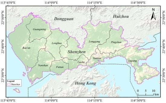
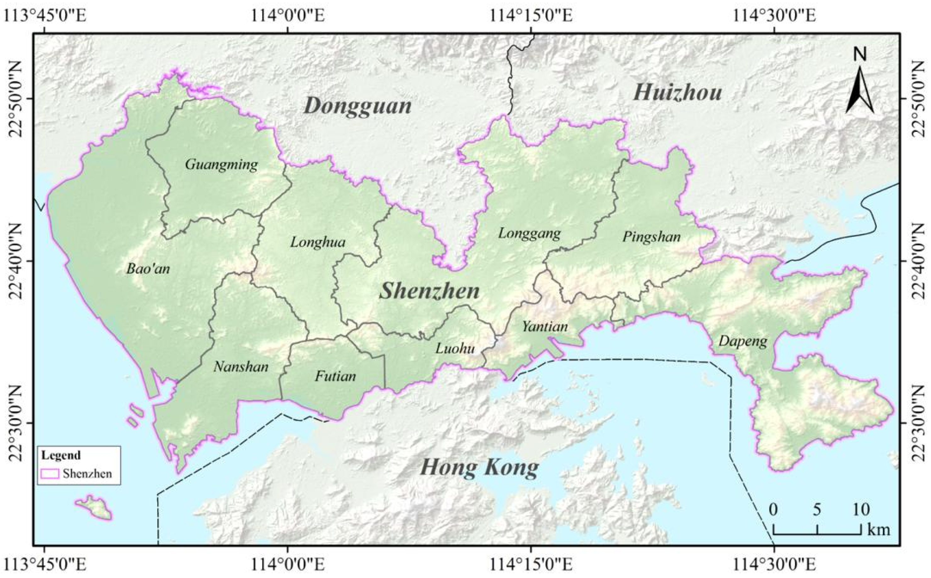
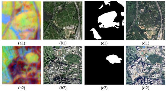
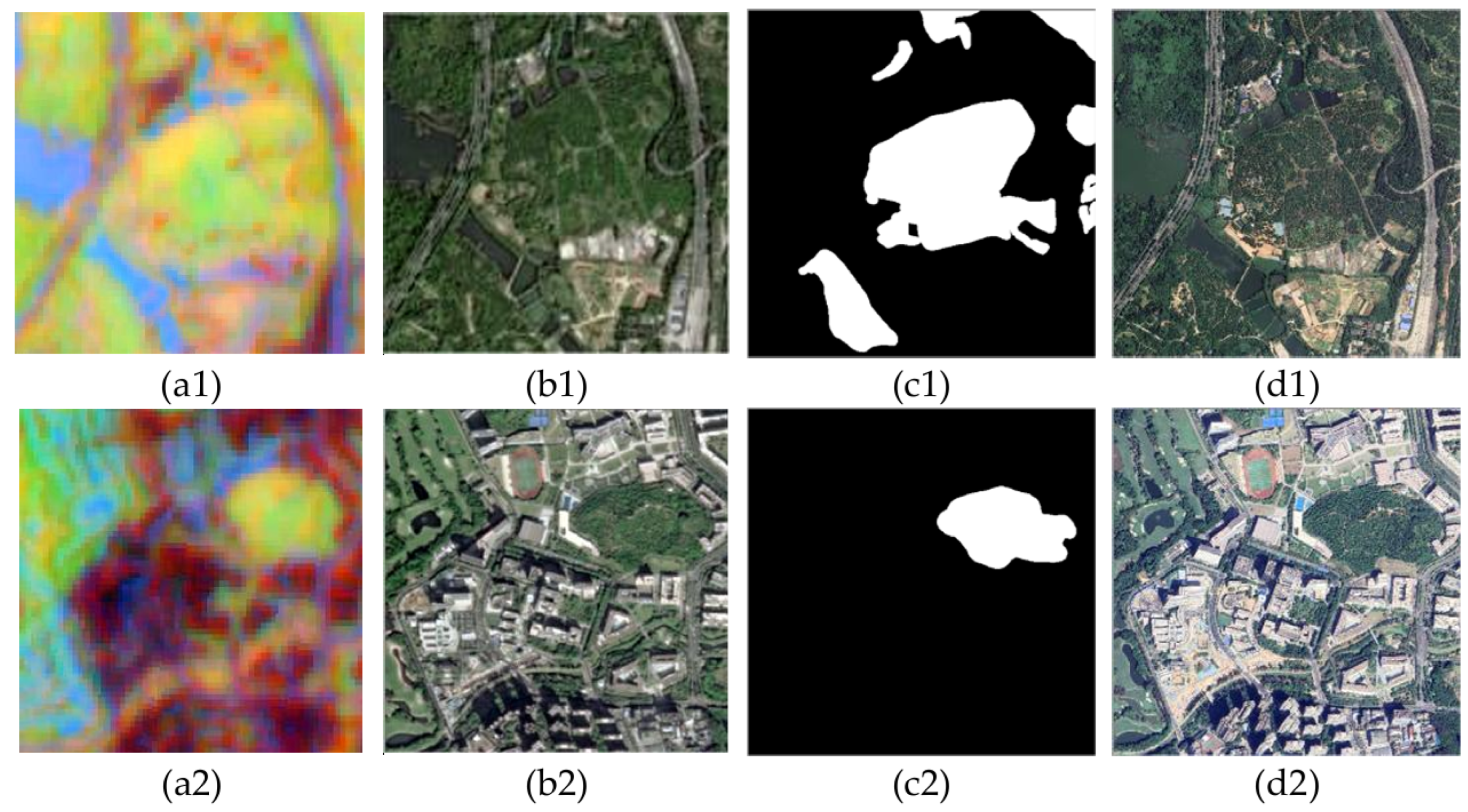
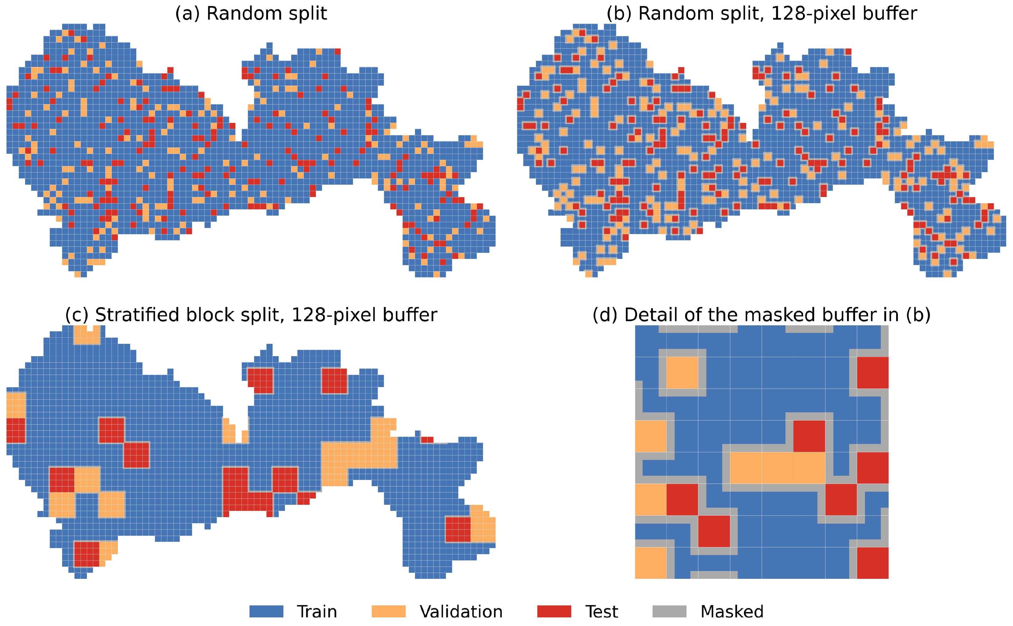
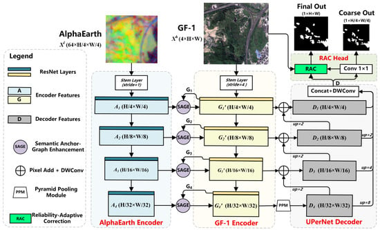
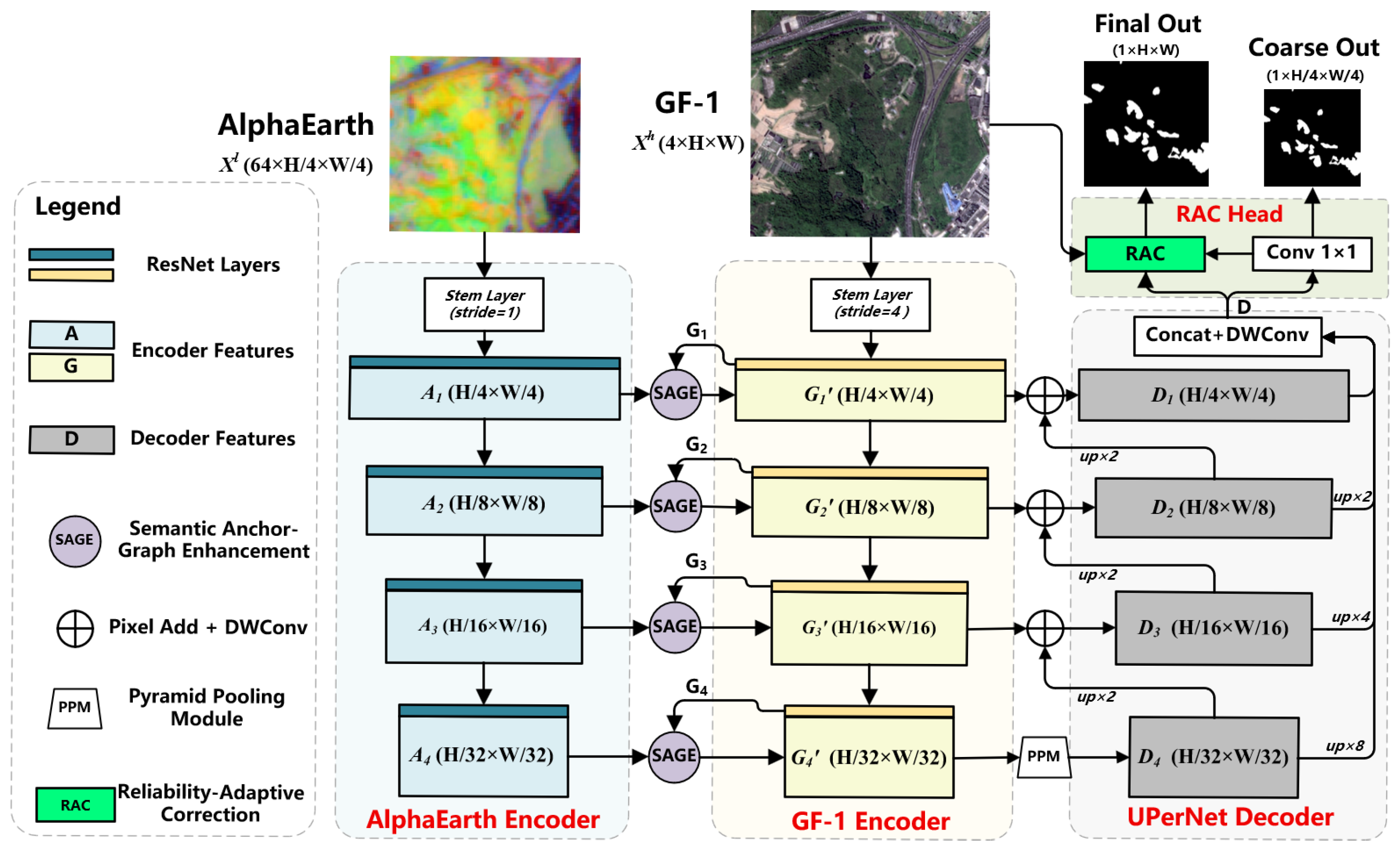
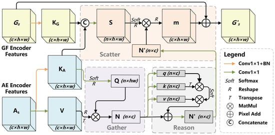
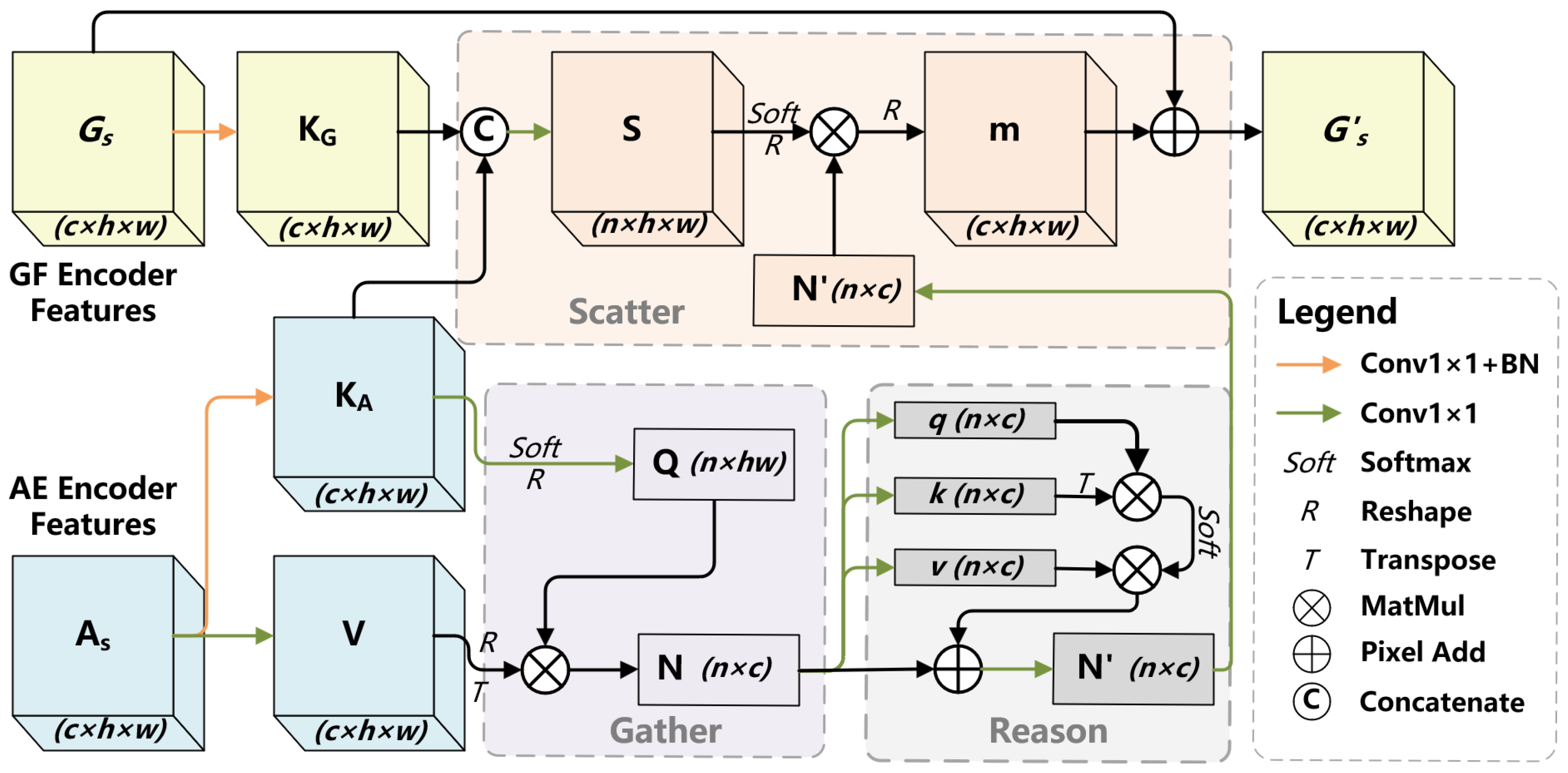
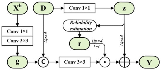
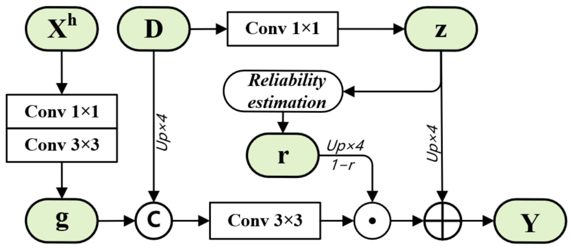
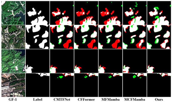
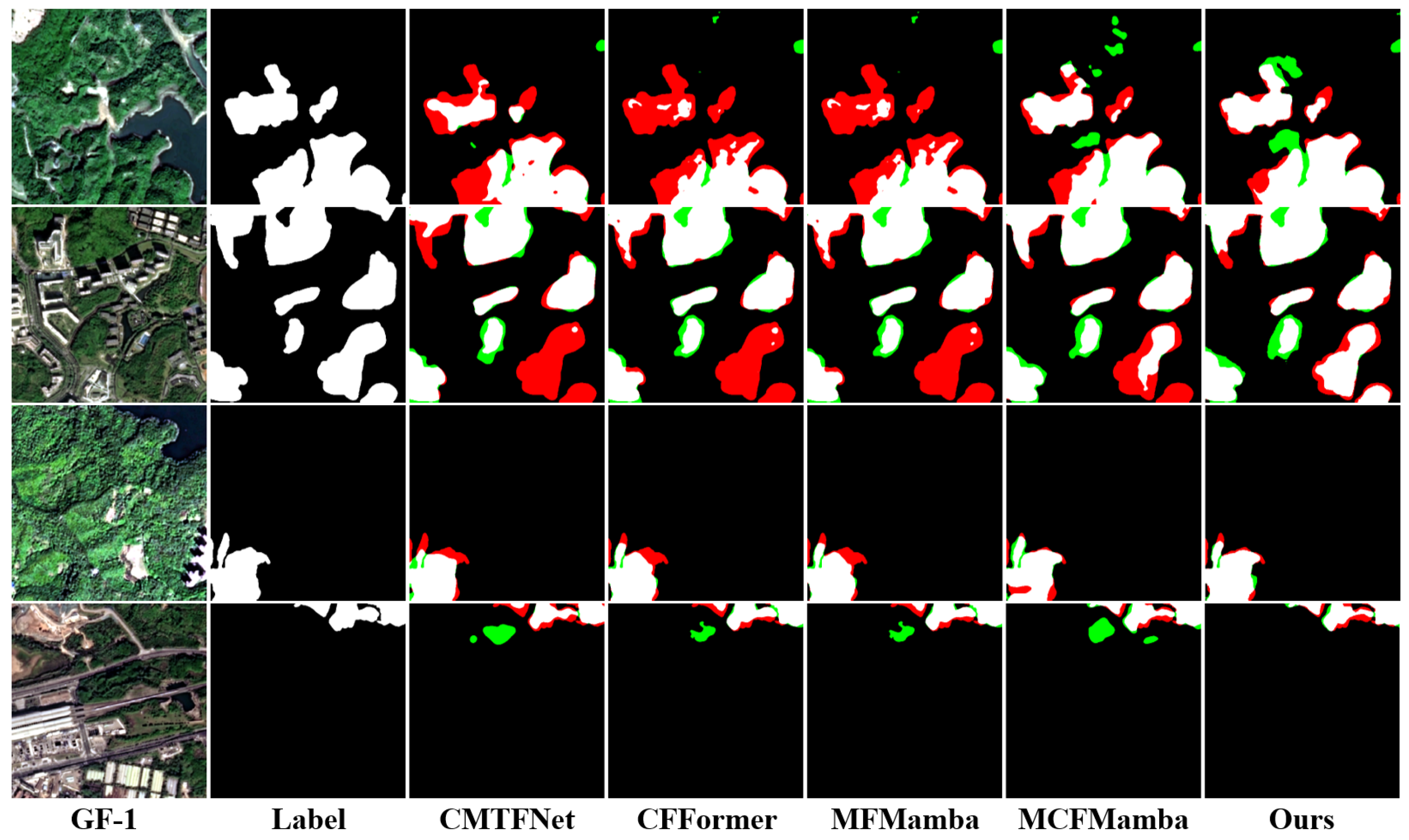
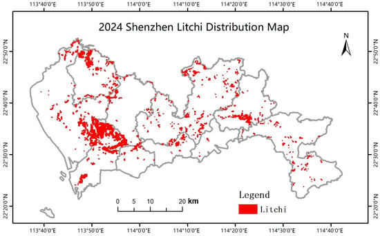
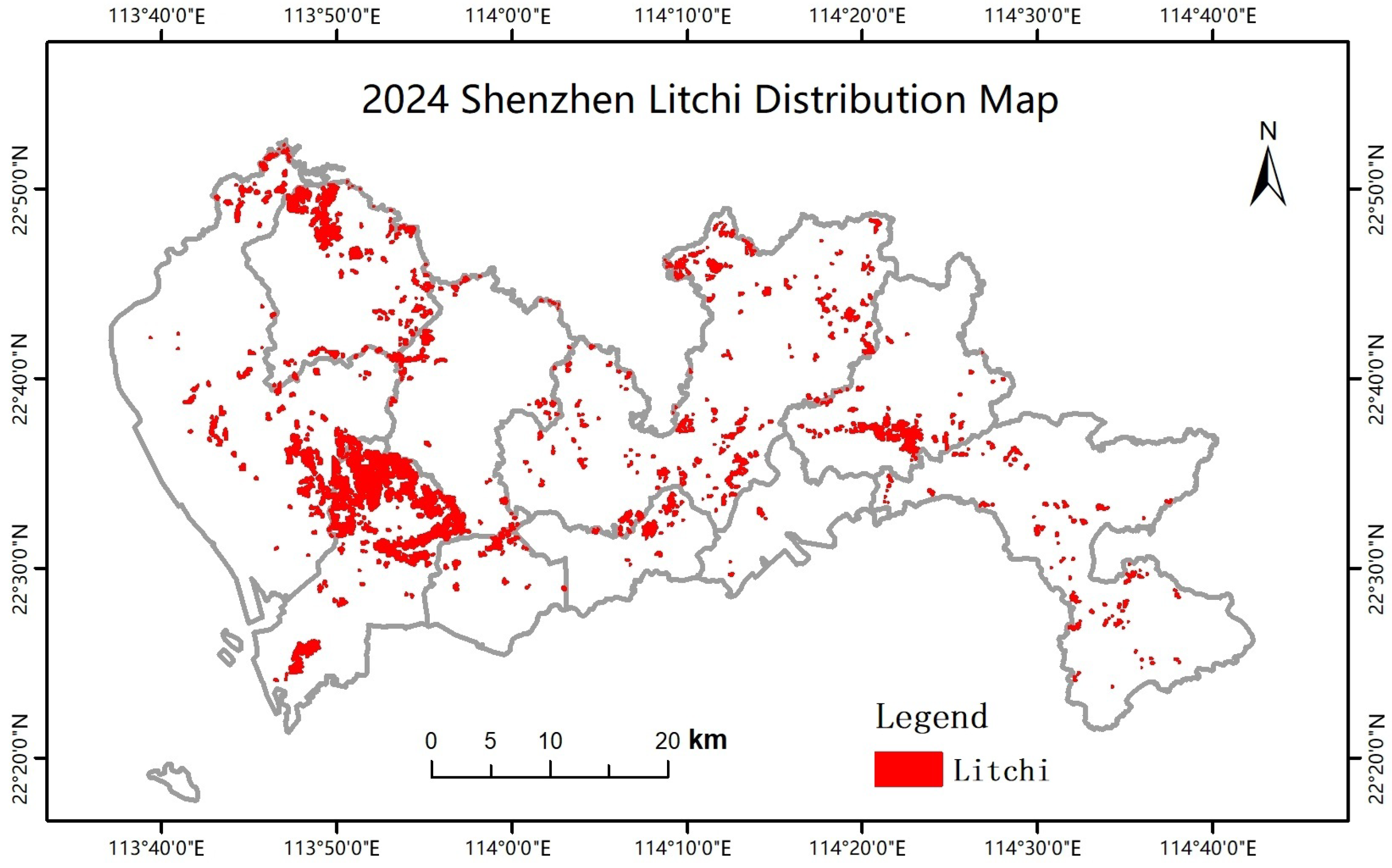
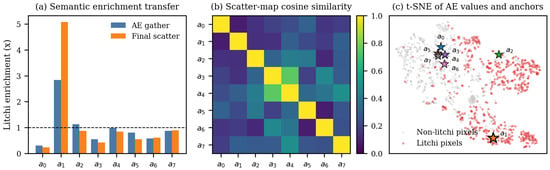
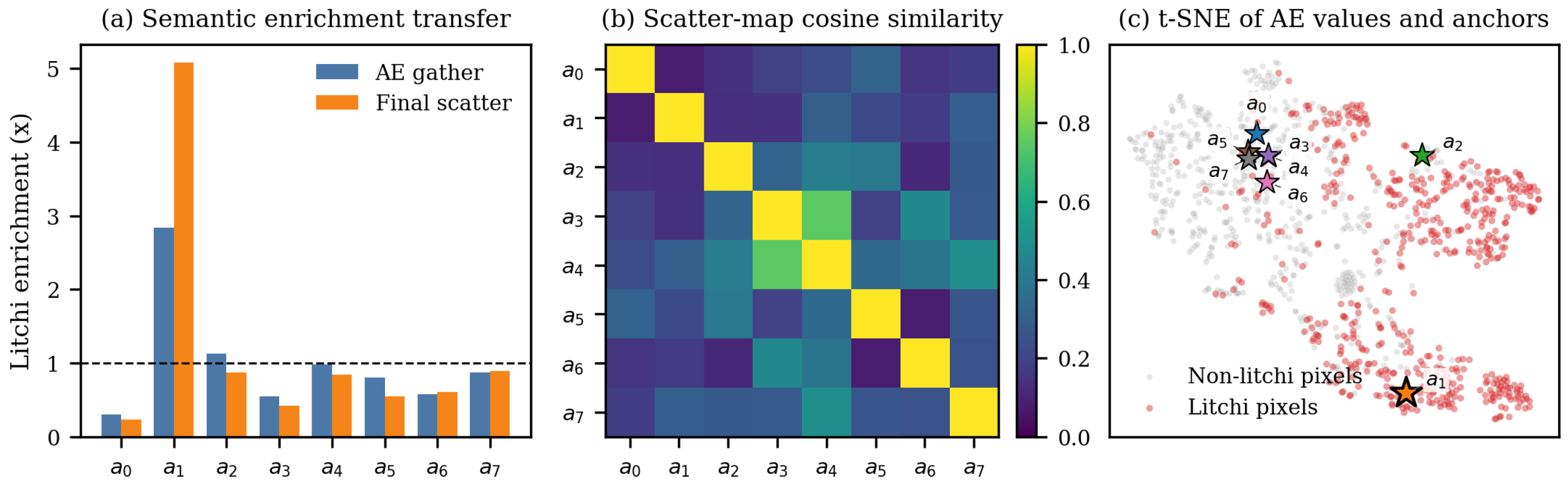
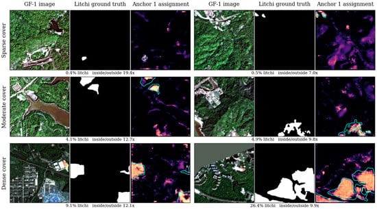
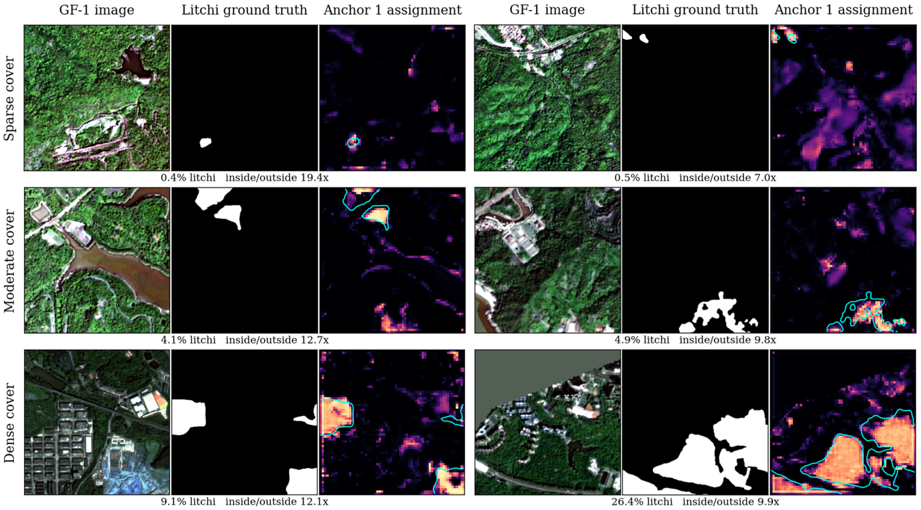
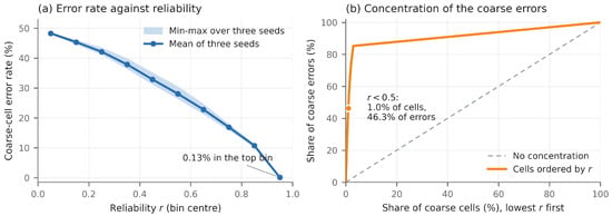
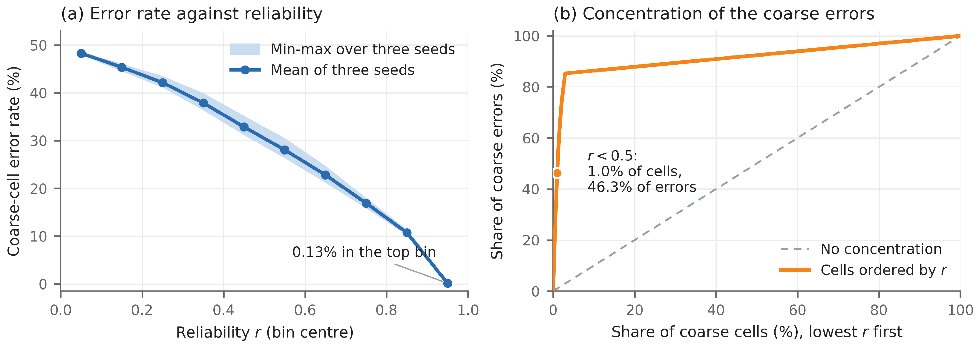

Disclaimer/Publisher’s Note: The statements, opinions and data contained in all publications are solely those of the individual author(s) and contributor(s) and not of MDPI and/or the editor(s). MDPI and/or the editor(s) disclaim responsibility for any injury to people or property resulting from any ideas, methods, instructions or products referred to in the content. |
© 2026 by the authors. Licensee MDPI, Basel, Switzerland. This article is an open access article distributed under the terms and conditions of the Creative Commons Attribution (CC BY) license.