SDFNet: Snow Depth Retrieval Based on a Multi-Scale Feature Fusion Network for the Qinghai-Tibet Plateau

Highlights

What are the main findings?

• Multi-source inputs reduced station-sample retrieval errors relative to single-source inputs.
• SDFNet achieved an RMSE of 5.246 cm and an R² of 0.702 in the station-based model comparison.

What are the implications of the main finding?

• FSC and terrain inputs improved SD estimates in the ablation comparisons.
• Independent spatial validation is required before applying the maps in poorly monitored mountains.

Abstract

High-resolution snow depth (SD) information supports hydrological and cryospheric studies in complex mountain regions. Coarse SD products limit representation of terrain-related snow variability in these environments. This study proposes SDFNet, a Snow Depth Fusion Network combining Sentinel-1 SAR, Landsat optical data, digital elevation model (DEM) variables, and fractional snow cover (FSC). Multi-scale feature extraction, channel enhancement, and feature aggregation modules represent relationships among these inputs. Observations from 95 meteorological stations across the Qinghai-Tibet Plateau supplied supervision and reference measurements for evaluation. Station SD was the regression target rather than a prediction input. In the station-based comparison, SDFNet achieved an RMSE of 5.246 cm and an R² of 0.702. It had the lowest RMSE and highest R² among the compared models. However, SD above 40 cm produced an RMSE of 21.927 cm and a bias of −16.061 cm, indicating substantial deep-snow underestimation. Sparse station coverage limits inference beyond the sampled environments, and independent spatial validation remains necessary.

1. Introduction

Snow cover is a major component of the surface hydrological system. It regulates winter surface temperature and supplies meltwater during the following warm season, making snow depth an important input for climate, hydrological, agricultural, and ecological models [1]. The Qinghai-Tibet Plateau, often referred to as the Roof of the World, is one of China’s main stable snow-covered regions and one of the regions most sensitive to climate change [2]. Snowmelt from the plateau and surrounding mountains strongly affects irrigation, infrastructure, ecosystems, and regional water security [3]. Accurate snow cover and snow depth mapping is therefore important for hydrology, remote sensing, and alpine ecosystem studies [4].

Field measurements of snow depth are difficult to obtain across snow-covered mountain regions because of harsh terrain and meteorological conditions. In situ observations are therefore sparse over both space and time [5]. Remote sensing provides an effective way to complement ground observations [6]. Optical and near-infrared imagery is useful for snow-cover monitoring, whereas microwave remote sensing is particularly valuable for snow-depth retrieval because microwave signals can penetrate the snowpack and are less affected by clouds and atmospheric conditions [7]. Passive microwave products are useful at broad scales [8] but usually have coarse spatial resolutions of approximately 1–25 km [9], which is insufficient for complex mountain terrain [10]. Synthetic aperture radar (SAR) offers higher spatial resolution and all-weather imaging capacity, making it suitable for alpine SD retrieval [11].

Deep learning has recently become widely used for high-resolution remote-sensing retrieval and image analysis [12]. Convolutional neural networks (CNNs) can learn spatial features directly from image data and reduce reliance on hand-crafted feature extraction [13]. For snow-depth mapping over the Qinghai-Tibet Plateau, Zhou et al. [14] combined FY-3B passive microwave observations with terrain, vegetation, and fractional snow-cover features, and used XGBoost to produce 500 m snow-depth estimates. Dunmire et al. [10] used Sentinel-1 C-band SAR data and XGBoost to estimate snow depth at 100 m resolution in the European Alps. These studies demonstrate the value of machine learning for alpine snow-depth retrieval, but shallow models have limited capacity for adaptive multi-source feature fusion in heterogeneous terrain.

Sentinel-based snow-depth retrieval has developed along both physical-model and data-driven paths. Lievens et al. used Sentinel-1 C-band SAR imagery to estimate snow depth and showed that time-series C-band SAR observations are informative for mountainous snow retrieval [15]. Feng et al. [16] further used dual-polarization Sentinel-1 data to improve snow-depth estimates in the Scandinavian Mountains. These studies indicate that SAR signals contain useful snow-depth information, but retrieval accuracy remains sensitive to terrain, snow conditions, and sensor-specific limitations.

A single sensor usually cannot balance spatial resolution, temporal coverage, and snow-depth sensitivity. SAR and optical imagery provide complementary information about surface scattering, snow albedo, and terrain-related snow distribution [17]. Multi-source fusion is therefore a promising strategy for improving snow-depth retrieval in complex alpine environments. Daudt et al. [18] fused optical, radar, and topographic data with deep learning to produce high-resolution snow-depth maps for Switzerland. Singh et al. [19] combined DInSAR and Landsat-9 data to estimate snow wetness and dielectric parameters for snow-depth modelling. These studies support multi-source fusion, but further work is needed for the Qinghai-Tibet Plateau, where terrain complexity, sparse station data, and heterogeneous snow conditions remain major challenges.

To address these limitations, this study develops SDFNet, a deep-learning model that fuses Sentinel-1 SAR data, Landsat optical data, DEM-derived terrain variables, and FSC information for snow-depth retrieval over the Qinghai-Tibet Plateau. The model is designed to enhance multi-scale spatial representation, adaptive channel weighting, and cross-scale feature aggregation under complex alpine conditions.

2. Materials and Methods

2.1. Study Area

The study area covers the Qinghai-Tibet Plateau, the world’s highest and one of its most topographically complex plateaus. The plateau includes high mountains, lakes, grasslands, and glaciers. It covers approximately 3.0834 million km², including about 2.5813 million km² within China, and has an average elevation of approximately 4400 m [20].

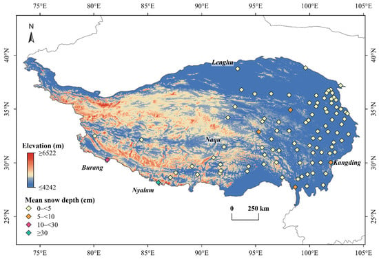
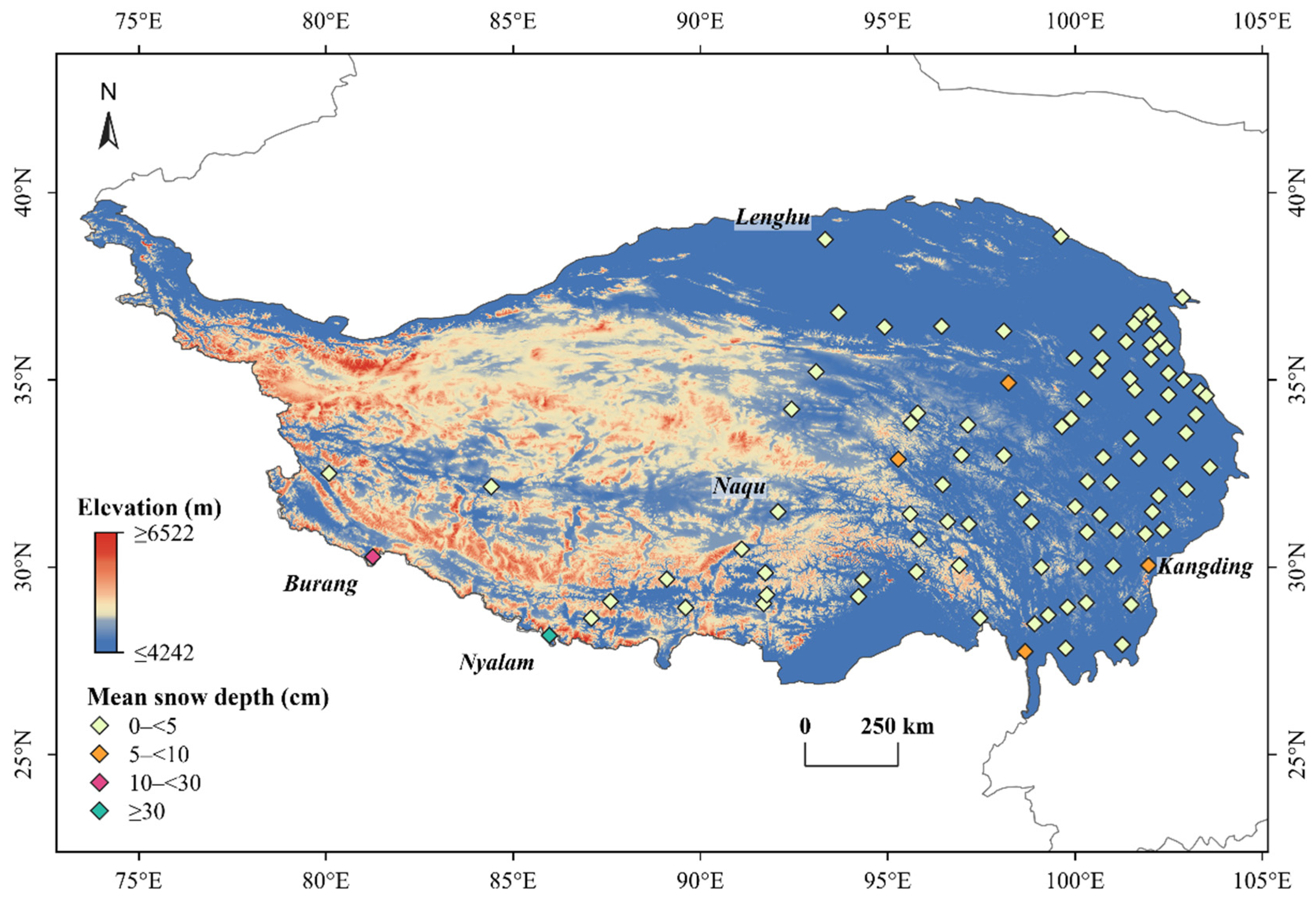
The meteorological stations are concentrated mainly along the eastern and northeastern parts of the plateau (Figure 1). Station coverage is limited in the western and central plateau and in high-elevation mountain environments. The available observations therefore support station-based evaluation but do not provide uniform validation of the entire study area.

Figure 1. Study area and distribution of the 95 meteorological stations on the Qinghai-Tibet Plateau. Diamond colours indicate mean observed snow depth, grouped as 0–<5, 5–<10, 10–<30, and ≥30 cm. Terrain colours represent DEM elevation and saturate below 4242 m and above 6522 m. Context boundary source: Esri World Countries (Generalized; Esri/Garmin/CIA/National Geographic).

2.2. Datasets and Preprocessing

2.2.1. Sentinel-1 GRD Data

Sentinel-1 provides freely available C-band SAR observations for land-surface monitoring [21]. This study used VV-polarized Sentinel-1A GRD data obtained from https://search.earthdata.nasa.gov/search (accessed on 10 October 2026). The data were pre-processed in SNAP 10.0 using orbit correction, noise removal, radiometric calibration, filtering, and terrain correction. The snow-season sampling window used for dataset construction is described in Section 3.1.

VV backscatter was used as the radar feature in this implementation and combined with optical, terrain, and FSC inputs. This choice defines the evaluated input configuration; it does not establish that VV is sufficient or preferable to dual-polarization observations. The implications of excluding VH, temperature, and temporal radar features are discussed in Section 5.4.

2.2.2. Landsat Data

Landsat-8 optical imagery supplied four visible and near-infrared input bands. The images were selected for the 2018, 2019, and 2020 snow seasons defined in Section 3.1 and combined with concurrent radar and station observations. The optical bands were reprojected to the common spatial reference and resampled from their 30 m resolution to the 10 m input grid for multi-source feature fusion. This resampling aligns the input grids but does not create independent optical observations at 10 m resolution.

2.2.3. In Situ Station Measurements

Daily in situ snow-depth observations were obtained from the National Meteorological Science Data Center (http://data.cma.cn/; accessed on 23 May 2025). The records include station identifiers, elevation, latitude and longitude, observation date, snow depth, snow pressure, and quality-control flags. After screening station IDs and geographic locations, 95 meteorological stations were retained for the study dataset. Only station records with concurrent satellite observations were used to construct labelled samples. Code 32766 denotes a missing observation, whereas code 32700 denotes trace snow and was treated as 0 cm. Samples with missing observations were excluded, as described in Section 3.1.

2.2.4. SRTM Elevation Data

SRTM elevation data were used for terrain correction during Sentinel-1 preprocessing and as auxiliary terrain information in the retrieval model. The data use the WGS84 spatial reference system [22] and were obtained from http://earthexplorer.usgs.gov/ (accessed on 10 October 2026). Slope and aspect were derived in ArcMap 10.8.

2.2.5. Fractional Snow Cover Data

Fractional snow cover (FSC) data were generated using the RepFNet-based FSC inversion approach developed in our previous study [23]. In that study, FY-4A/AGRI remote-sensing observations and Landsat-8 OLI imagery were used to retrieve FSC, and the resulting FSC information was used here as an auxiliary snow-cover prior for SDFNet snow-depth retrieval.

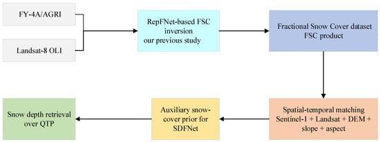
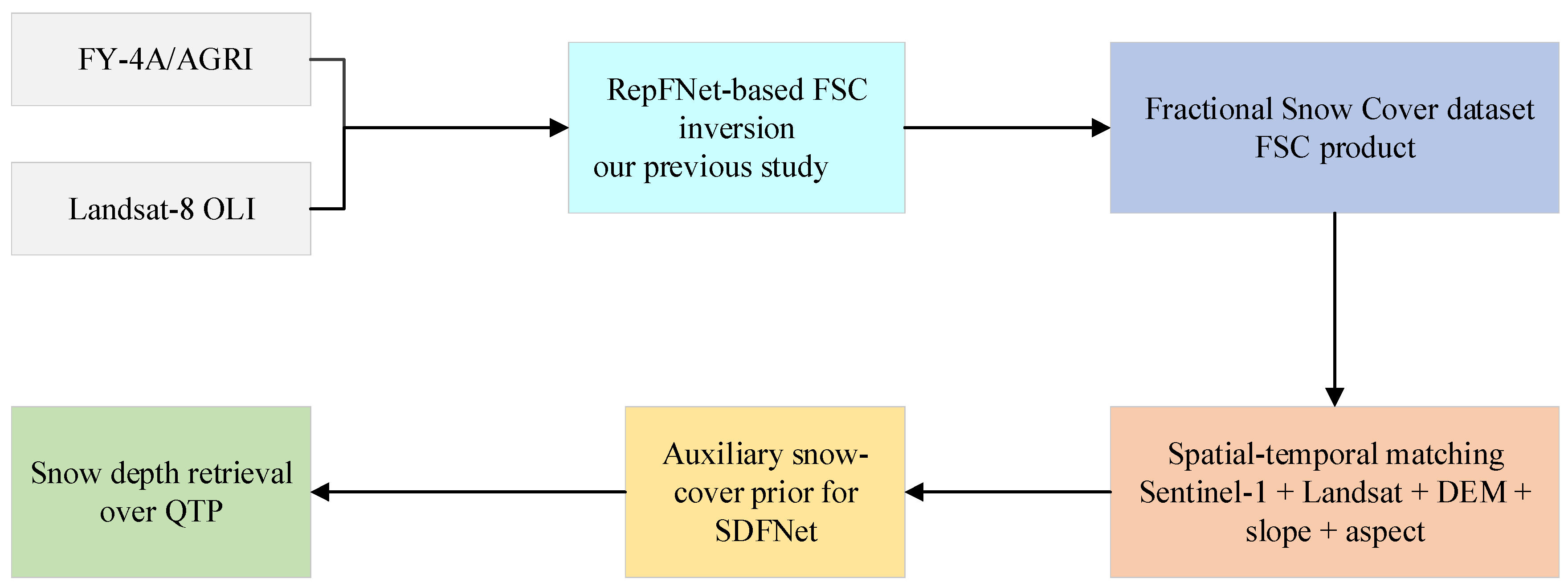
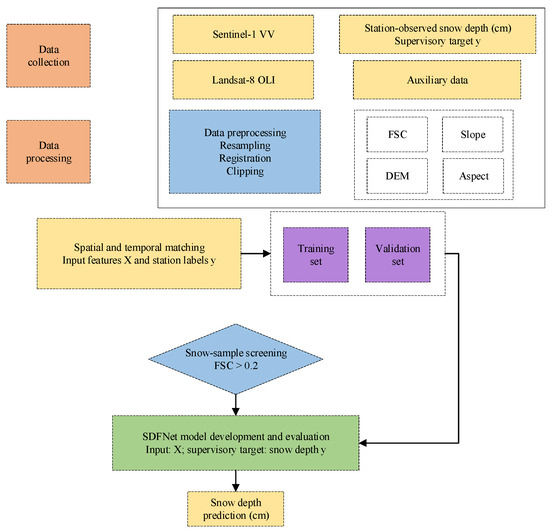
The generation and application framework of the FSC dataset used in this study is shown in Figure 2. The FSC dataset was generated from FY-4A/AGRI observations and Landsat-8 OLI imagery using the RepFNet-based inversion method developed in our previous study [23]. The generated FSC data were then spatially and temporally matched with Sentinel-1 SAR observations, Landsat optical data, DEM-derived terrain variables, and station-based snow-depth samples. In SDFNet, FSC was used as an auxiliary snow-cover prior to improve the representation of snow-cover heterogeneity and support high-resolution snow-depth retrieval over the Qinghai-Tibet Plateau.

Figure 2. Generation and application framework of the FSC dataset used in this study. The RepFNet-based FSC retrieval method was developed in our previous study [23].

2.3. Dataset Construction

Sentinel-1 SAR observations were combined with Landsat optical data and auxiliary variables within the sampling window described in Section 3.1. The VV-polarized SAR band was selected after orbit correction, noise removal, radiometric calibration, filtering, and terrain correction. DEM, slope, aspect, and FSC were used as auxiliary inputs. Station-centred boundary files were generated to clip the overlapping raster layers. The fused input was reported to contain 11 channels, with station-observed SD used as the target variable rather than an input channel.

3. Methodology

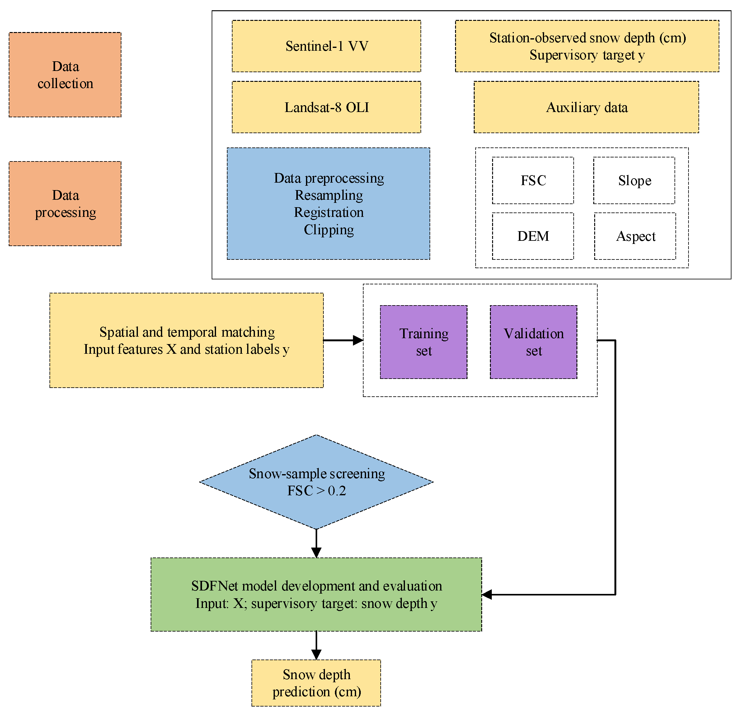
The workflow in Figure 3 links satellite preprocessing, station-observation matching, and supervised SD estimation. Sentinel-1, Landsat, terrain, and FSC observations supplied the model input features. Daily SD measured at the corresponding station supplied the regression target for each matched sample. The resulting image patches were used to train SDFNet, and model estimates were compared with station observations using the metrics in Section 3.3. Station SD observations were not supplied as prediction-time input features.

Figure 3. Workflow of SDFNet, with station-observed snow depth as the supervised regression target. Colors distinguish workflow components and do not represent quantitative values.

3.1. Data Preprocessing

The dataset covered the 2018, 2019, and 2020 snow seasons. Each season is named by its starting year and extends from 1 October to 31 March of the following year. The 2018, 2019, and 2020 seasons therefore correspond to 1 October 2018 to 31 March 2019, 1 October 2019 to 31 March 2020, and 1 October 2020 to 31 March 2021, respectively. Sentinel-1 and Landsat observations were integrated with DEM-derived variables and FSC information. Sentinel-1 VV-polarized observations and four Landsat visible and near-infrared bands were pre-processed to a common projection and resampled to a 10 m grid. Station-centred 32 × 32 pixel patches were matched with concurrent station SD records. Each patch therefore covered a 320 m × 320 m neighbourhood, while its supervisory target was a point-scale station observation. Samples affected by cloud contamination, invalid pixels, or missing observations were excluded. Approximately 10,000 samples with the reported 11-channel input and corresponding station SD labels were constructed. Dataset partitioning is described in Section 3.3.

3.2. SDFNet Model Construction

Multi-scale feature extraction and contextual representation are critical for snow-depth retrieval from remote-sensing images. Terrain, illumination, land cover, and local redistribution processes cause snow features to vary across spatial scales. Conventional convolutional networks may not adequately balance local texture and broader spatial context. SDFNet was therefore designed around multi-kernel dynamic fusion and context enhancement. The network includes a feature extraction module, a channel enhancement module, and a multi-scale feature aggregation module to improve the representation of heterogeneous snow-depth patterns. The overall network architecture is shown in Figure 4.

Figure 4. Overall architecture of the SDFNet model. Colors distinguish computational blocks and schematic feature maps; they do not indicate numerical feature values.

3.2.1. Feature Extraction Module (FEM)

The Feature Extraction Module (FEM) was designed to capture multi-scale snow-depth signals in alpine terrain. Snow-depth patterns vary with macro-topographic relief, local wind redistribution, slope aspect, and microtopographic shading. Windward and leeward slopes can show metre-scale differences in snow accumulation, whereas valleys and ridges affect snow retention at broader spatial scales. A retrieval model must therefore represent both local snow texture and larger terrain-controlled patterns.

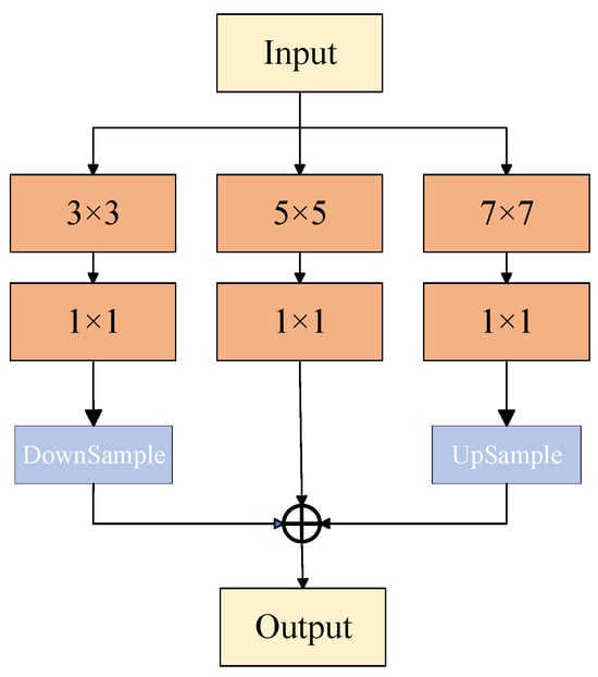
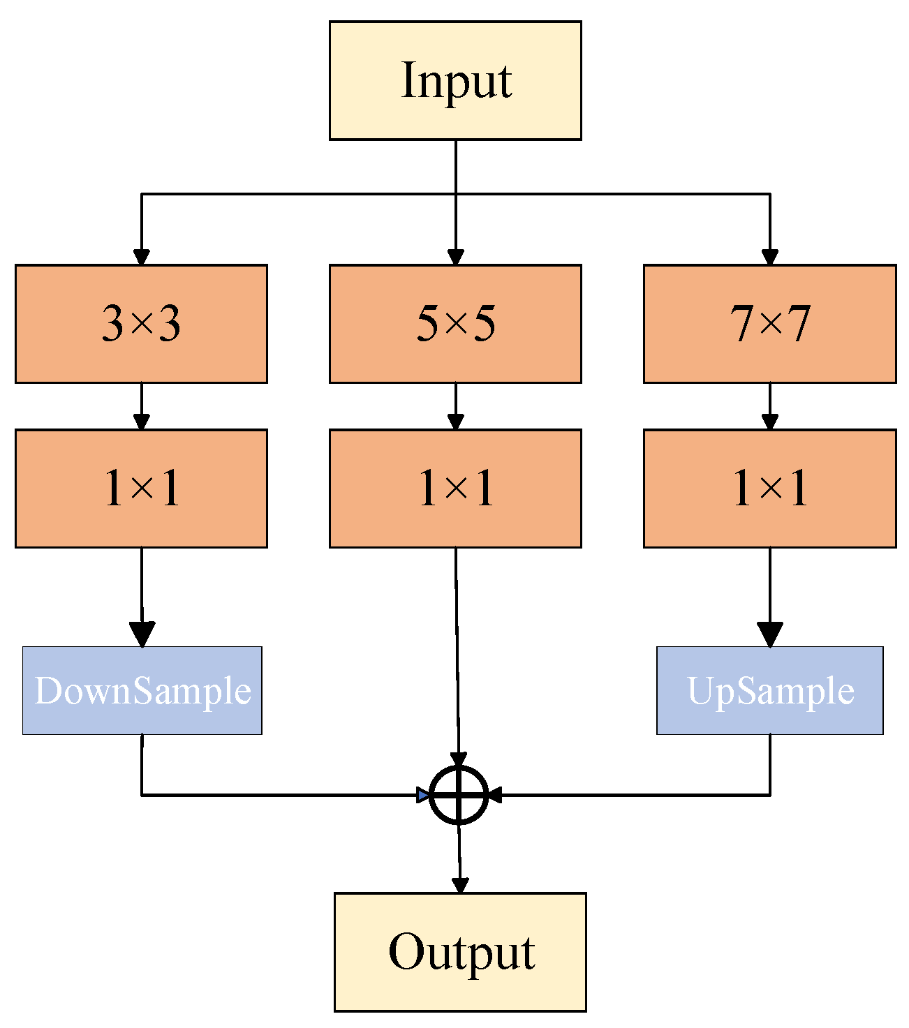
FEM uses parallel 3 × 3, 5 × 5, and 7 × 7 convolution branches to capture local texture, mesoscale structure, and broader spatial variation (Figure 5). A 1 × 1 convolution follows each branch to compress and align channel dimensions, reducing computational cost while preserving scale-specific information. Bilinear interpolation is used when needed to align feature-map sizes before concatenation. The fused multi-scale representation improves sensitivity to terrain relief and snow texture under complex mountain conditions.

Figure 5. Structure of the Feature Extraction Module (FEM).

3.2.2. Channel Enhancement Module (CEM)

Snow distribution in high-resolution remote-sensing imagery is spatially heterogeneous because of wind, terrain relief, slope aspect, vegetation, and land-cover differences. Snow thickness can differ between windward and leeward slopes, snowdrifts may form in local depressions, and exposed rock or vegetation can interrupt continuous snow cover. Snow-depth retrieval therefore requires both spatial-scale representation and feature-channel discrimination.

Different land-cover types also have distinct spectral reflectance and microwave scattering responses. Optical bands are sensitive to snow albedo, whereas microwave bands respond to snow structure, liquid water content, and snow thickness. Terrain shadow, sensor noise, and local occlusion can weaken single-channel information. Modelling correlations and complementarities among channels is therefore necessary to enhance physically meaningful snow-depth features.

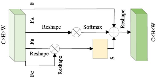
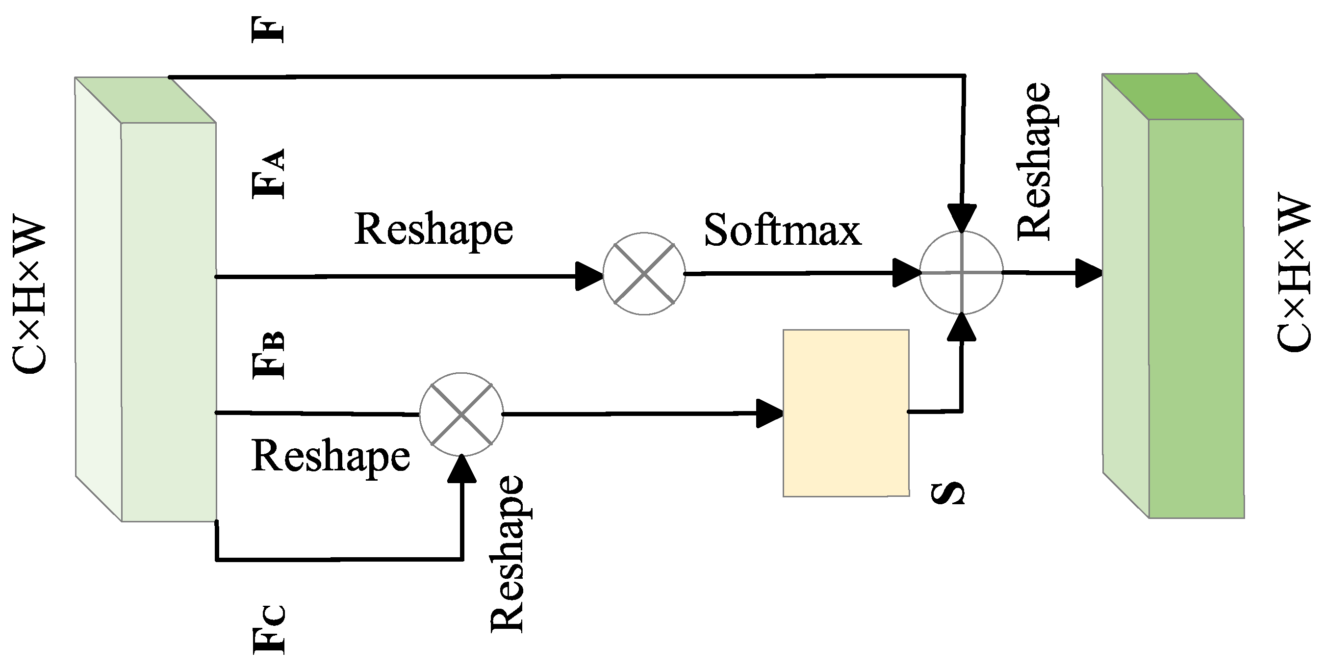
The Channel Enhancement Module (CEM) adaptively models dependencies among feature channels (Figure 6). It summarizes global channel responses, learns the contribution of each channel to snow-depth variation, and assigns dynamic channel weights. This process emphasizes spectral or scattering channels that are more informative for snow-depth retrieval and suppresses noisy or redundant responses.

Figure 6. Structure of the Channel Enhancement Module (CEM).

The input feature tensor F ∈ ℝ^C×H×W is flattened along its spatial dimensions to obtain channel-level representations, as shown in Equation (1).

{F_A, F_B, F_C} ∈ R^C×N, N = H × W

(1)

To represent the dependencies between different feature channels, the channel correlation matrix S is computed, as shown in Equation (2).

$$S=F_B\cdot F_C^{\mathrm{T}}$$

(2)

Softmax normalization is applied to the correlation matrix along the channel dimension to obtain the channel dependency weight matrix A, where each element is calculated as shown in Equation (3).

$$A_{\mathit{ij}}={\displaystyle \frac{\exp (S_{\mathit{ij}})}{{\displaystyle {\sum }_{j=1}^{\mathrm{C}}\exp (S_{\mathit{ij}})}}}$$

(3)

Here, A_ij represents the response intensity of the i-th channel to the j-th channel and characterizes dependencies among feature channels. The original channel features are reweighted and reconstructed using the channel-dependency weights. A learnable scale parameter is then introduced, and the reconstructed features are mapped back to the original spatial dimensions for residual fusion with the input features, as shown in Equation (4).

$$E=\gamma \cdot {\displaystyle {\sum }_{i=1}^{\mathrm{C}}(A_{\mathit{ij}}{S}_i)+S_j}$$

(4)

The scale parameter is initialized to 0 at the beginning of training, allowing the model to learn the importance of channel dependencies gradually. This design stabilizes training while adaptively enhancing discriminative feature channels for snow-depth retrieval.

3.2.3. Multi-Scale Feature Aggregation Module (MFAM)

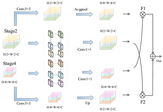
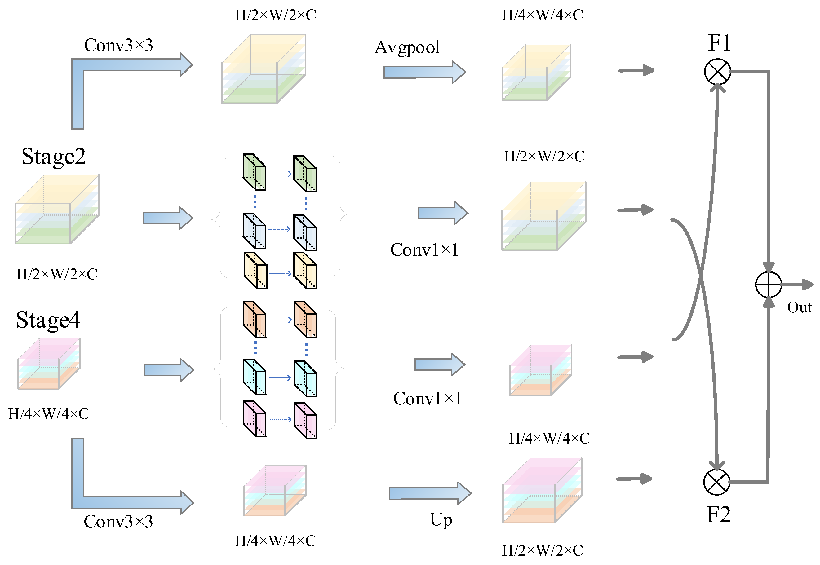
Multi-source remote-sensing inputs differ in spatial resolution and spectral response, and features at different scales provide complementary information for characterizing snow-depth patterns. The Multi-scale Feature Aggregation Module (MFAM) integrates mid- and high-level encoder features through multi-path convolution and pooling operations, enabling cross-scale fusion and deeper representation of multi-modal snow-depth information.

MFAM uses a multi-branch structure to model features at different scales. Channel dimensions from different downsampling stages are first aligned using 1 × 1 convolutions. Local structure is then modelled using 3 × 3 convolution and depthwise separable convolution. An element-wise multiplicative attention mechanism strengthens correlations between cross-scale features and aggregates shallow detail features with deeper semantic features.

In Figure 7, C, W, and H denote the channel count, width, and height of feature maps, respectively. C_1×1 and C_3×3 denote convolutions with kernel sizes of 1 and 3. B denotes batch normalization, C_d denotes depthwise convolution, Up denotes upsampling, and Ap denotes average pooling. The corresponding calculations are given in Equations (5)–(7).

F₁ = C_1×1{B[C_d(X₁)]} · Sigmoid{Up[B(C_3×3(X₂))]}

(5)

F₂ = Ap{B[C_3×3(X₁)]} · Sigmoid{C_1×1[B(C_d(X₂))]}

(6)

$${\mathit{Out}=B\{C}_{3\times 3}\left[{F_1+\mathit{Up}(F}_2\right)]$$

(7)

Figure 7. Structure of the Multi-scale Feature Aggregation Module (MFAM). Colored cuboids schematically represent feature maps at the indicated stages; the colors do not encode feature magnitudes.

3.3. Accuracy Evaluation Metrics

Samples from the 2018 and 2019 snow seasons were used for training and validation, whereas the 2020 snow season was reserved for an independent temporal test. This season-based separation assesses performance in a different period; it does not by itself establish generalization to unseen stations or regions. Model performance was assessed using the coefficient of determination (R²), root mean square error (RMSE), mean absolute error (MAE), bias (BIAS), positive mean error (PME), and negative mean error (NME).

$$R^2=1-{\displaystyle \frac{{\displaystyle {\sum }_{i=1}^n{(y_i-{\widehat{y}}_i)}^2}}{{\displaystyle {\sum }_{i=1}^n{(y_i-\overline{y})}^2}}}$$

(8)

$$\mathit{RMSE}=\sqrt{{\displaystyle \frac{1}{n}}{\displaystyle \sum _{i=1}^n{(y_i-{\widehat{y}}_i)}^2}}$$

(9)

$$\mathit{BIAS}={\displaystyle \frac{1}{N}}{\displaystyle \sum _{i=1}^N({\widehat{y}}_i-y_i)}$$

(10)

$$\mathit{MAE}={\displaystyle \frac{1}{n}}{\displaystyle \sum _{i=1}^n\left|y_i-{\widehat{y}}_i\right|}$$

(11)

$$\mathit{PME}={\displaystyle \frac{1}{p}}{\displaystyle \sum _{i=1}^p({\widehat{y}}_i-y_i)},{\widehat{y}}_i>y_i$$

(12)

$$\mathit{NME}={\displaystyle \frac{1}{q}}{\displaystyle \sum _{i=1}^q({\widehat{y}}_i-y_i)},{\widehat{y}}_i<y_i$$

(13)

Here, y_i is observed station SD, ${\widehat{y}}_i$ is estimated SD, $\overline{y}$ is mean observed SD, and n (N in Equation (10)) is the number of samples. In Equations (12) and (13), p and q count samples with positive and negative errors, respectively. RMSE and MAE quantify error magnitude, while BIAS measures the mean signed error. Lower RMSE and MAE, and an absolute BIAS closer to zero, indicate lower errors. Positive BIAS denotes overestimation, whereas negative BIAS denotes underestimation of observed SD. PME and NME summarize mean errors conditional on their positive and negative signs, respectively. RMSE, MAE, BIAS, PME, and NME are expressed in centimetres; R² is dimensionless.

4. Results

All experiments were conducted on a workstation with an Intel Core i9-14900KF CPU (Intel Corporation, Santa Clara, CA, USA), 32 GB of RAM, and an NVIDIA GeForce RTX 4090 GPU (NVIDIA Corporation, Santa Clara, CA, USA) with 24 GB of VRAM. Python 3.8.19 and PyTorch 2.4.1+cu121 were used for model implementation. The Adam optimizer was used with an initial learning rate of 1 × 10⁻³ and a batch size of 64. Models were trained for up to 300 epochs, with early stopping when validation loss did not improve for 20 consecutive epochs. The learning rate was reduced by a factor of 0.1 when validation loss increased.

4.1. FSC Threshold Selection

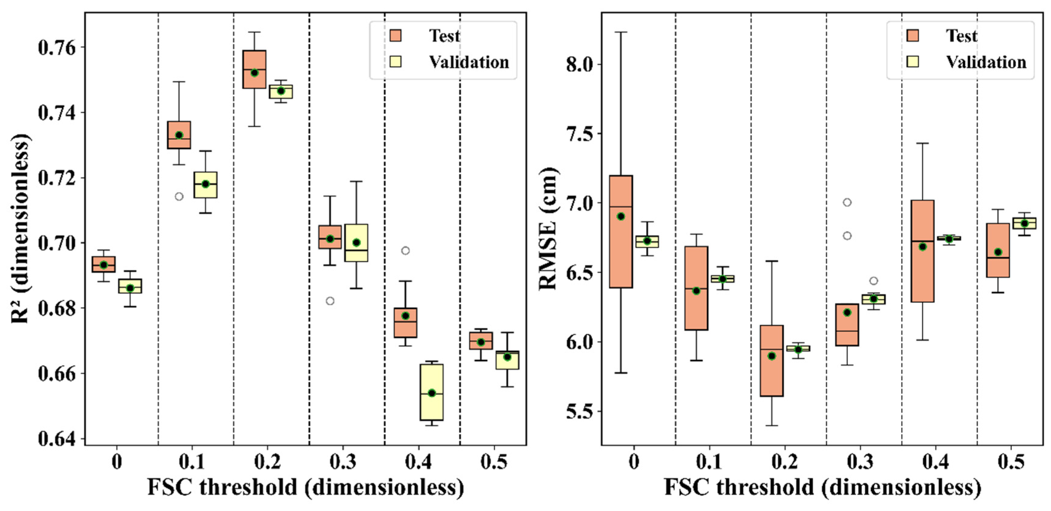
FSC was used as a prior constraint to identify snow-covered pixels and reduce interference from snow-free or trace-snow samples. An initial threshold of FSC > 0 retained many trace or mixed pixels, which increased uncertainty between station labels and remote-sensing features. We therefore evaluated several FSC thresholds to identify a threshold that improved sample quality while retaining enough training samples.

FSC ∈ {0, 0.1, 0.2, 0.3, 0.4, 0.5}

(14)

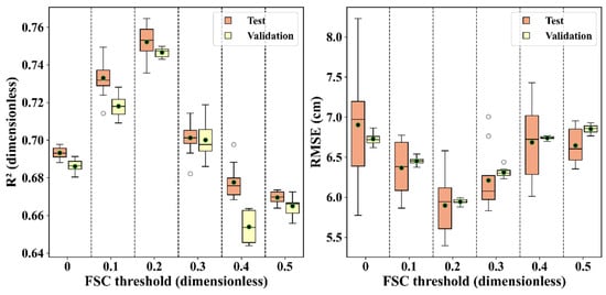
For each threshold, pixels with FSC above the threshold were retained as valid snow samples. SDFNet was trained and evaluated under identical model and training settings for each dataset. Validation accuracy metrics were then compared across thresholds (Figure 8).

Figure 8. FSC threshold selection experiment results. Green-outlined circles mark mean values.

The threshold experiment compared FSC values of 0, 0.1, 0.2, 0.3, 0.4, and 0.5. FSC thresholds and R² are dimensionless, whereas RMSE is expressed in centimetres. The configuration with FSC > 0.2 gave the most favourable combination of R² and RMSE among the tested thresholds. Increasing the threshold further did not improve the reported accuracy, and FSC > 0.2 was selected for snow-sample screening. This screening defines the evaluated sample population and should not be interpreted as validation of performance at every snow-cover fraction. Mixed pixels and threshold selection are known considerations in optical snow-cover estimation [24,25,26].

4.2. Ablation Experiments

4.2.1. Data-Source Ablation

Data-source ablation experiments compared the contribution of the input groups under the reported model settings. The full input comprised Sentinel-1 SAR, Landsat optical data, and auxiliary DEM, slope, aspect, and FSC variables. Five configurations were compared: SAR only; SAR with auxiliary variables; SAR with Landsat; Landsat with auxiliary variables; and all three input groups. RMSE, MAE, BIAS, and R² were reported for 500 samples drawn from the 2020 independent test season. These ablation results describe this sampled evaluation and are distinguished from the overall model comparison in the following model-comparison section.

Auxiliary inputs comprise DEM, slope, aspect, and FSC. RMSE, MAE, and BIAS are expressed in centimetres; R² is dimensionless. BIAS is the mean estimated minus observed snow depth, so negative values indicate underestimation.

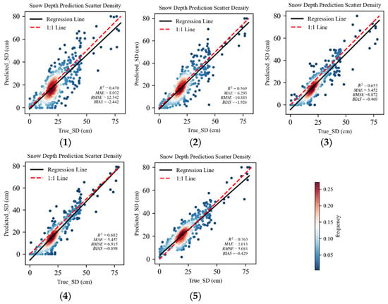
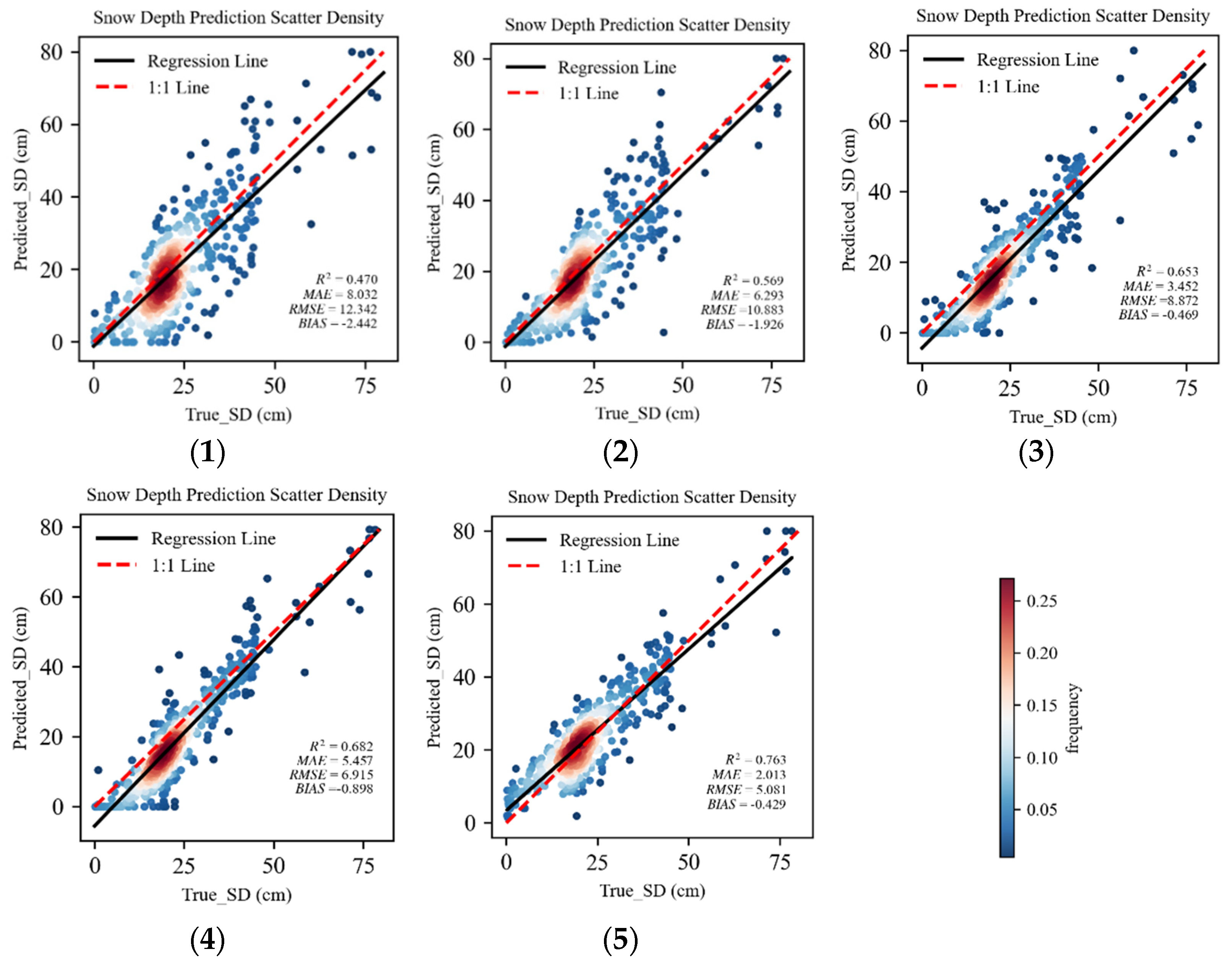
In Table 1, the SAR-only configuration had the largest reported RMSE, at 12.342 cm, with an R² of 0.470. Adding auxiliary variables reduced RMSE to 10.883 cm, while combining SAR with Landsat reduced it to 8.872 cm, with an R² of 0.653. Landsat with auxiliary variables gave an RMSE of 6.915 cm and an R² of 0.682. The full input gave an RMSE of 5.081 cm, an MAE of 2.013 cm, and an R² of 0.763. This sample-based comparison supports the benefit of combining the input groups. The corresponding observed-versus-estimated scatter-density plots are presented in Figure 9.

Table 1. Station-sample evaluation of the data-source ablation configurations.

Method	RMSE (cm)	MAE (cm)	BIAS (cm)	R2
SAR	12.342	8.032	−2.442	0.470
SAR + Auxiliary Data	10.883	6.293	−1.926	0.569
SAR + Landsat	8.872	3.452	−0.469	0.653
Landsat + Auxiliary Data	6.915	5.457	−0.898	0.682
SAR + Landsat + Auxiliary Data	5.081	2.013	−0.429	0.763

Figure 9. Observed versus estimated snow depth for the Table 1 configurations: (1) SAR; (2) SAR + auxiliary; (3) SAR + Landsat; (4) Landsat + auxiliary; (5) SAR + Landsat + auxiliary. Auxiliary inputs are DEM, slope, aspect, and FSC.

4.2.2. FSC Feature Ablation

The FSC ablation compared two input configurations on the reported evaluation sample set. Both configurations used Sentinel-1 SAR, Landsat optical data, DEM, slope, and aspect under the same model architecture. The experimental configuration additionally included FSC, whereas the control configuration excluded this feature. The comparison isolates the reported difference between these two input configurations.

Including FSC improved all evaluation metrics (Table 2). The result indicates that FSC provides useful spatial information about snow distribution and helps the model characterize snow-depth variability more accurately.

Table 2. Station-sample evaluation with and without the FSC input.

Method	R2	RMSE (cm)	BIAS (cm)	MAE (cm)
SAR + Landsat + terrain auxiliary data	0.734	6.432	−0.827	4.219
SAR + Landsat + terrain auxiliary data + FSC	0.763	5.081	−0.429	2.013

4.2.3. Network-Module Ablation

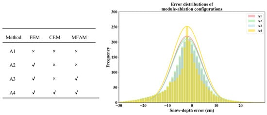
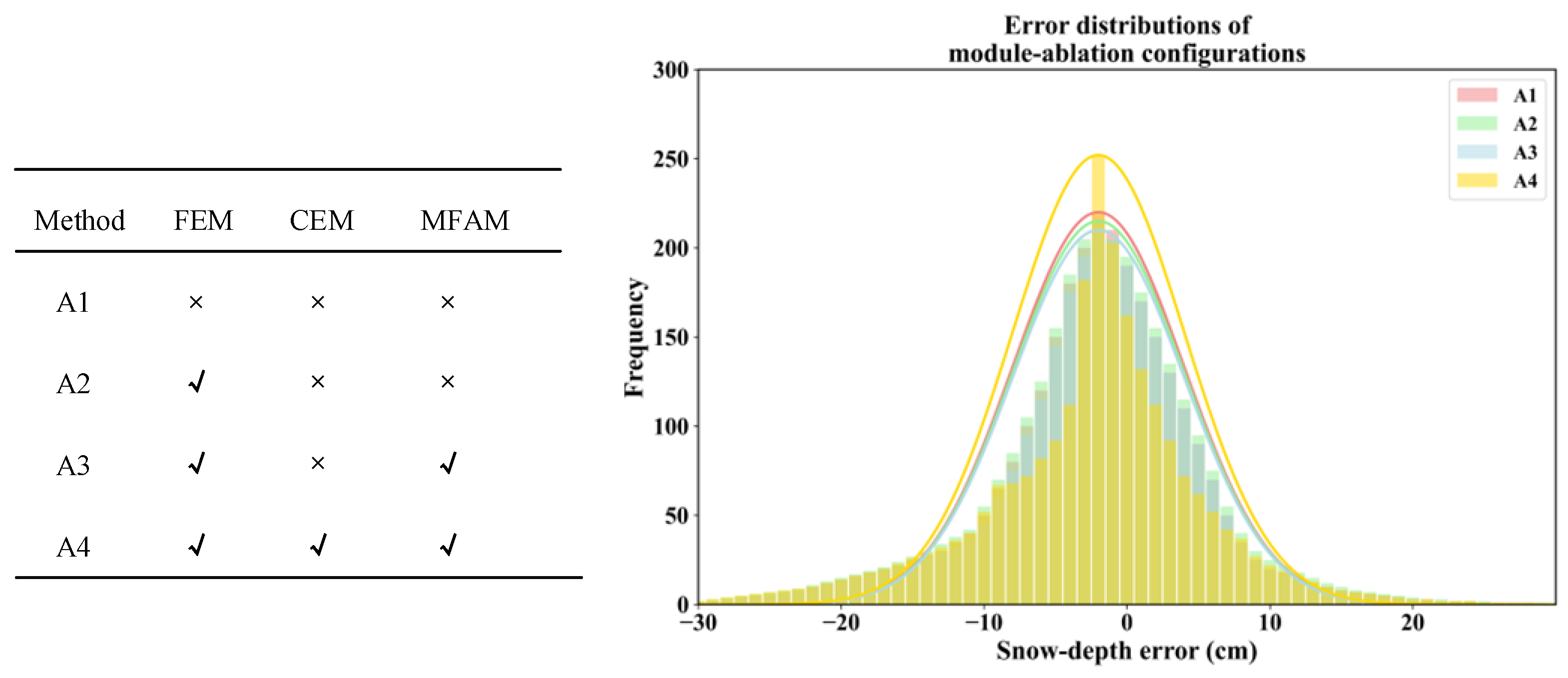
A stepwise model ablation experiment was conducted to quantify the contribution of FEM, CEM, and MFAM. ResNet was used as the baseline, and the proposed modules were added sequentially under the same data and training settings. Changes in BIAS distributions were compared to assess the effect of each module on snow-depth retrieval error (Figure 10).

Figure 10. BIAS distribution results of module ablation experiment. In the configuration table, check marks denote included modules and crosses denote omitted modules. A1 is the baseline; A2 includes FEM; A3 includes FEM and MFAM; and A4 includes FEM, CEM, and MFAM.

Figure 10 compares the error distributions of configurations A1–A4 under the reported module-ablation settings. The full configuration A4 includes FEM, CEM, and MFAM, and its distribution is more concentrated near zero than the baseline distribution. This comparison describes the observed error distributions but does not establish robustness across unobserved terrain or snow conditions.

4.3. Comparison with Baseline Models

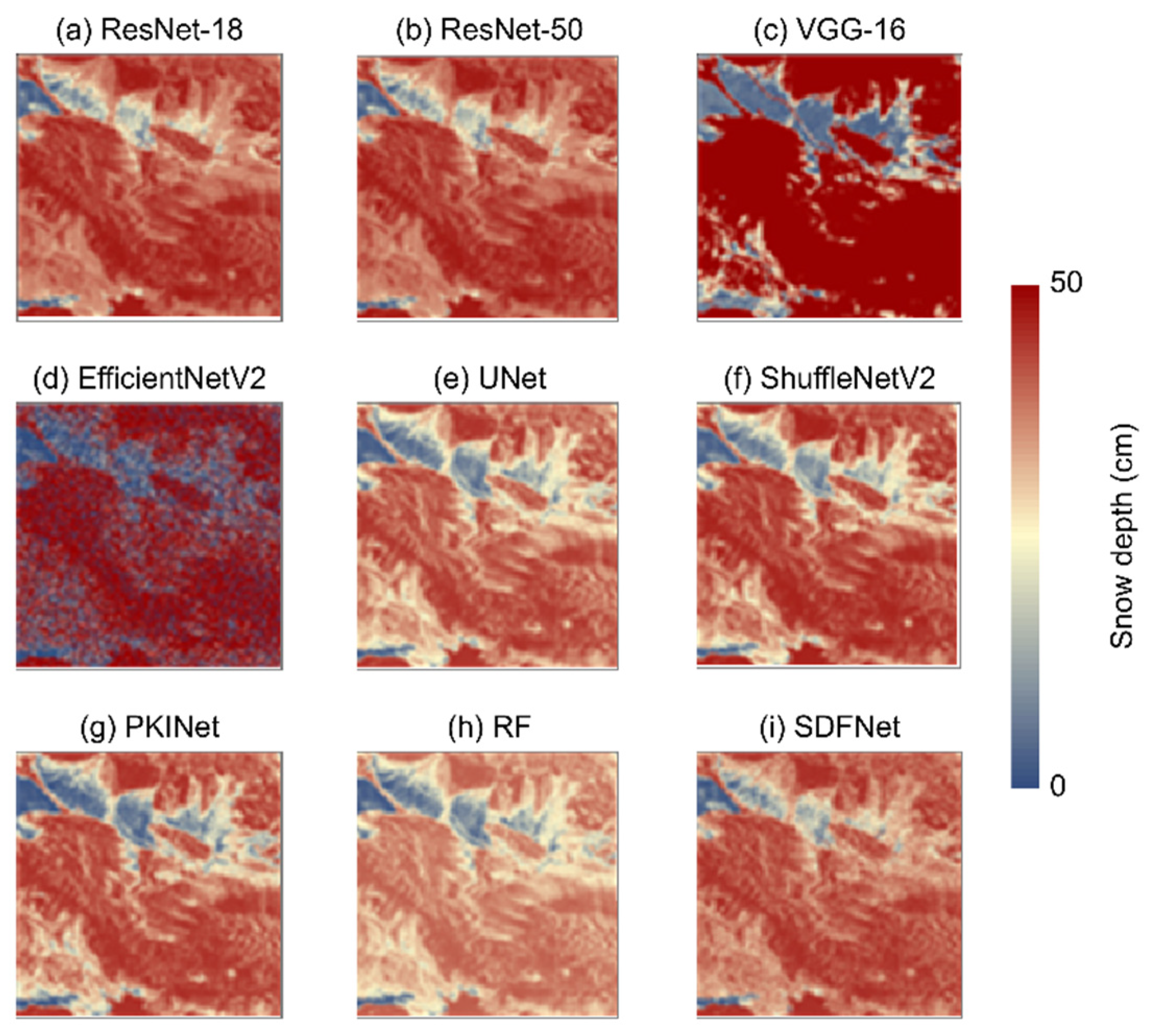
SDFNet was compared with ResNet [27], VGG16 [28], EfficientNetV2 [29], UNet [30], ShuffleNetV2 [31], PKINet [32], and random forest (RF) [33]. The compared methods used the same dataset and preprocessing pipeline, with the reported training and evaluation partitions kept consistent. The neural-network models used Adam and the same loss function; this optimization description does not apply to RF. Quantitative station-sample results are reported in Table 3, while Figure 11 illustrates the estimated spatial patterns.

Table 3. Station-sample snow-depth retrieval errors for the compared methods.

Method	RMSE (cm)	MAE (cm)	BIAS (cm)	R2	PME (cm)	NME (cm)
ResNet-18	8.352	4.351	−0.527	0.682	1.324	−1.923
ResNet-50	7.573	5.047	−0.713	0.619	1.372	−1.724
VGG-16	10.352	4.603	1.307	0.634	1.393	−2.041
EfficientNetV2	9.784	4.690	−0.821	0.606	2.961	−2.731
UNet	7.363	5.332	1.473	0.592	2.081	−2.363
ShuffleNetV2	8.367	4.442	−2.091	0.651	2.022	−2.937
PKINet	7.235	3.064	0.826	0.652	1.621	−2.641
RF	7.874	4.236	0.324	0.625	1.848	−2.784
SDFNet	5.246	2.452	−0.642	0.702	0.924	−1.823

Figure 11. Qualitative comparison of local snow-depth retrieval patterns from the nine models.

SDFNet had the lowest RMSE and MAE and the highest R² among the methods in Table 3. Its RMSE was 5.246 cm, compared with 7.235 cm for PKINet, the next-lowest RMSE. This difference represents a 27.5% reduction in RMSE relative to PKINet on the reported evaluation samples. SDFNet also had a mean bias of −0.642 cm, indicating residual underestimation rather than complete removal of systematic error. It did not minimize every signed-error metric, and its overall advantage should not be interpreted as uniform superiority across snow-depth ranges.

The local image patches in Figure 11 illustrate differences in spatial smoothness and local variability among model estimates. Without an independent spatial snow-depth reference, these differences cannot identify which map is most accurate. The quantitative comparison in Table 3 therefore supports performance at the sampled stations rather than accuracy at every mapped location. Fine spatial texture alone does not demonstrate improved retrieval accuracy in unobserved mountain areas.

5. Discussion

5.1. Retrieval Accuracy Across Snow-Depth Ranges

SDFNet performance was further evaluated across snow-depth intervals. Evaluation samples were grouped by observed snow depth, and accuracy metrics were calculated for each interval (Table 4).

Table 4. Snow-depth retrieval errors grouped by observed station snow depth.

Snow Depth Range (cm)	RMSE (cm)	MAE (cm)	BIAS (cm)
0–10	3.123	2.147	1.035
10–20	4.361	4.298	−2.150
20–30	6.325	5.541	−3.219
30–40	7.651	7.254	−7.168
>40	21.927	19.201	−16.061

Depth groups are defined by station observations. All reported error metrics are in centimetres, and negative BIAS indicates underestimation.

Errors increased as observed SD increased, with a transition from shallow-snow overestimation to pronounced deep-snow underestimation (Table 4). For 0–10 cm snow, RMSE was 3.123 cm and BIAS was +1.035 cm, indicating a positive mean error. For 10–20 cm snow, RMSE increased to 4.361 cm and BIAS became −2.150 cm. BIAS decreased further to −3.219 cm and −7.168 cm in the 20–30 cm and 30–40 cm groups, respectively. For SD above 40 cm, RMSE reached 21.927 cm, MAE reached 19.201 cm, and BIAS was −16.061 cm. These errors indicate a substantial limitation in deep-snow estimation that is obscured by the aggregate RMSE of 5.246 cm.

Several processes could contribute to the deep-snow errors, but the present experiments do not separate their effects. C-band VV backscatter can be weakly sensitive to dry-snow accumulation and strongly affected by wet-snow absorption [15]. Optical reflectance and FSC describe surface and snow-cover conditions rather than independently measuring snowpack thickness. Limited depth sensitivity, an uneven distribution of training samples, and station-to-patch representativeness are therefore possible contributors to underestimation. Their contributions require sample counts by depth, snow-state information, and controlled feature comparisons. The 40 cm grouping boundary in Table 4 is an evaluation interval, not a demonstrated physical saturation threshold for C-band SAR.

5.2. Time-Series Comparison

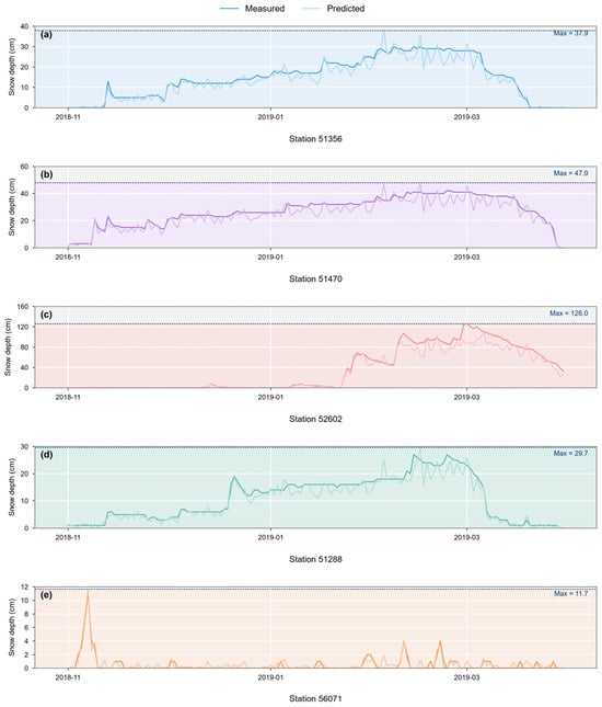
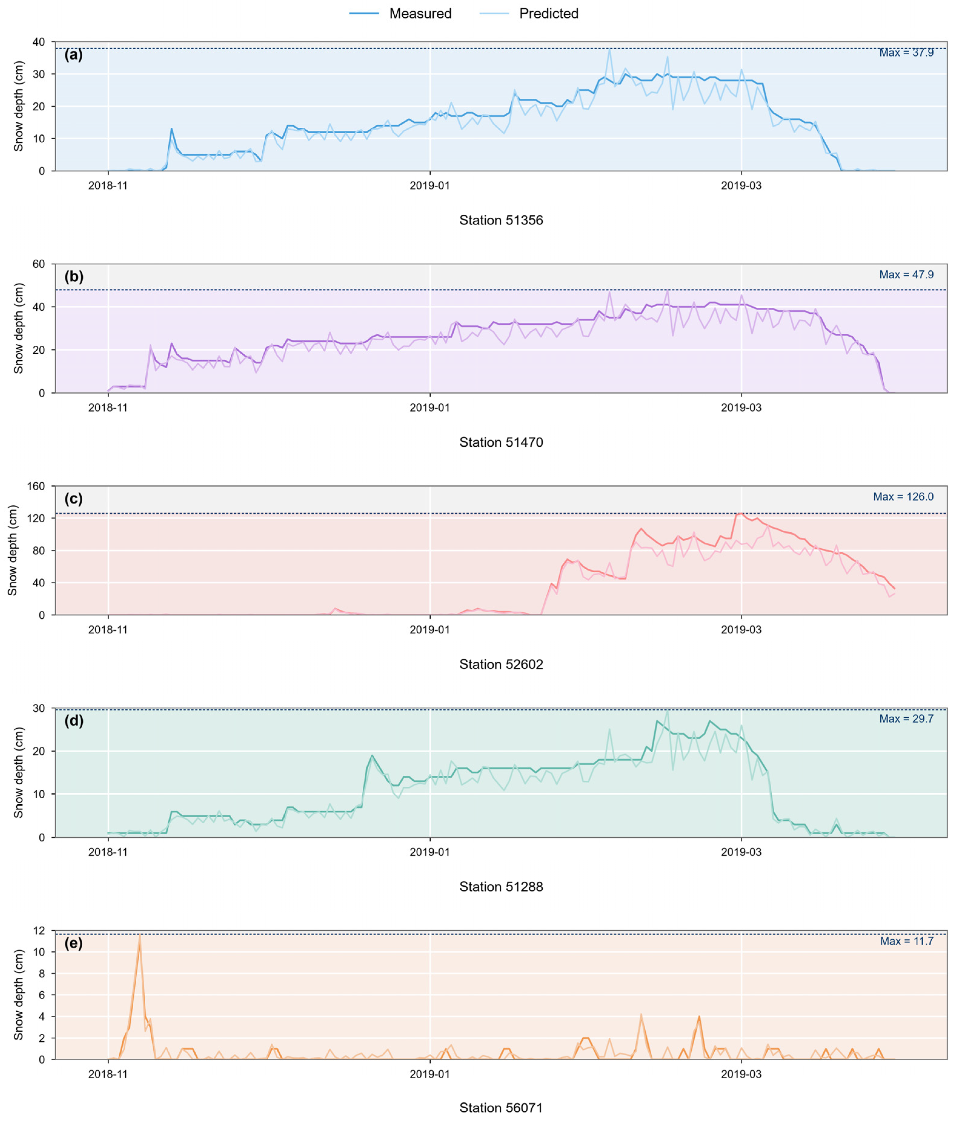
Figure 12 compares estimated and observed SD at five selected meteorological stations during the illustrated 2018–2019 period. The curves show seasonal accumulation and melt, together with deviations in individual peaks and underestimation in the deeper-snow example. These examples illustrate temporal behaviour at the selected stations and complement the depth-stratified errors in Table 4. They do not by themselves establish performance in independent seasons, at unseen stations, or across the full mapped area.

Figure 12. Comparison of observed and estimated snow-depth time series at five selected meteorological stations. Panels show stations (a) 51356, (b) 51470, (c) 52602, (d) 51288, and (e) 56071. In each panel, the horizontal dashed line indicates the maximum value across the observed and predicted snow-depth series during the plotted period.

5.3. Spatial Distribution of Retrieval Error

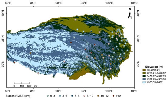
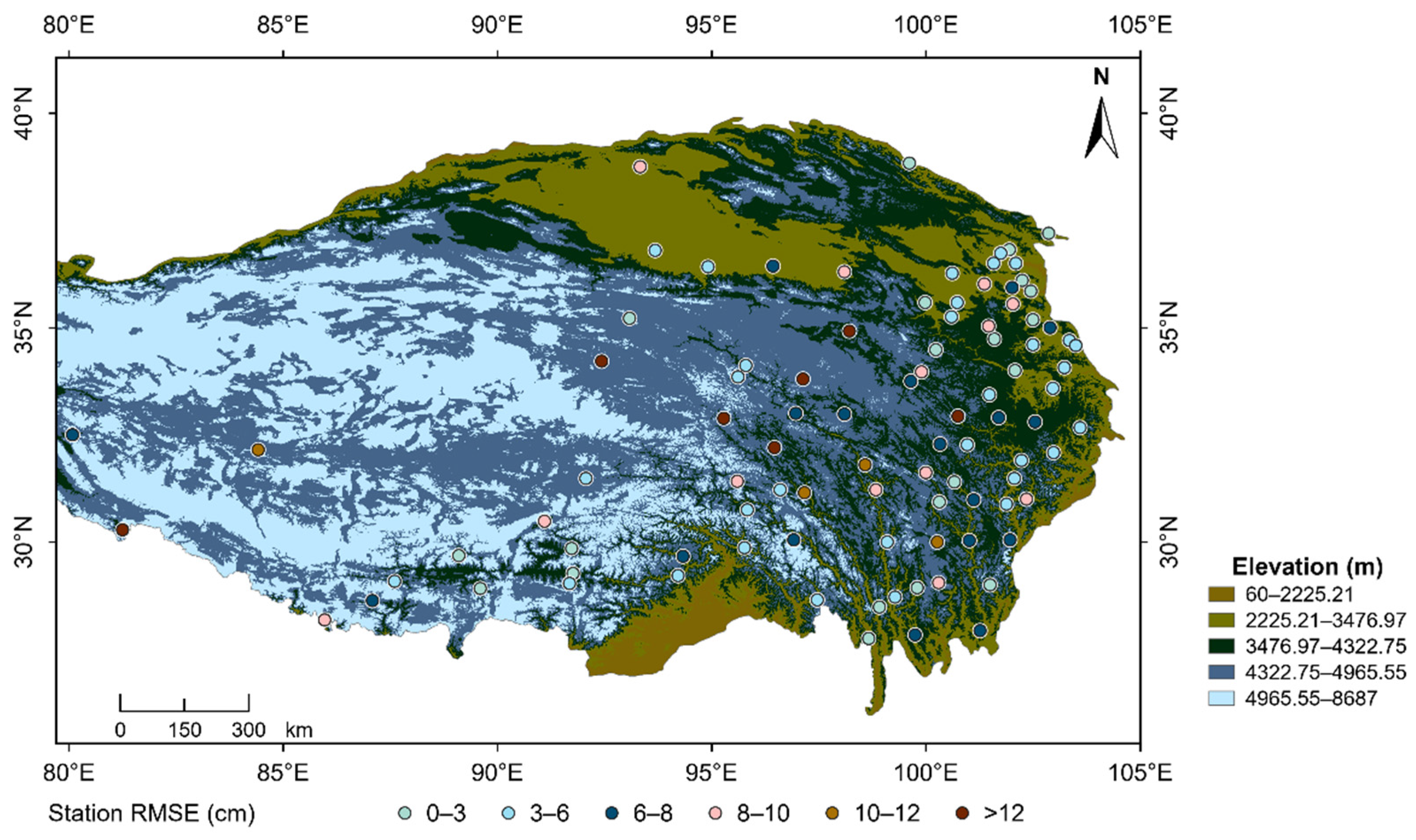
Figure 13 summarizes station-level RMSE in six plotted classes: 0–3, 3–6, 6–8, 8–10, 10–12, and >12 cm. The station symbols are overlaid on elevation to show the locations of the reported errors. These values represent errors at observation sites rather than a continuously validated error surface for the plateau.

Figure 13. Spatial distribution of station-level snow-depth RMSE overlaid on elevation. Circle colours indicate station-level RMSE classes (cm); the background represents elevation (m).

The mapped stations show spatial variation in RMSE, but the network is concentrated along the eastern and northeastern parts of the study area. Western, central, and high-elevation mountain environments have limited observational representation in the available station network (Figure 1 and Figure 13). Consequently, low errors at observed stations cannot establish accuracy in poorly monitored terrain. Differences in snow conditions, terrain, and point-to-patch representativeness may affect the spatial error pattern, but their effects were not independently quantified. Additional observations are needed to evaluate these explanations and the reliability of estimates beyond the sampled environments.

5.4. Observation and Validation Limitations

The use of point-scale station labels is a central limitation of spatial snow-depth estimation. A 32 × 32 input patch provides neighbourhood context, but one station observation does not describe snow depth at every pixel. Resampling Landsat and terrain inputs to a 10 m grid also does not create independent observations at that scale. The station-based metrics and maps should therefore be interpreted at their respective observational supports.

Only VV-polarized radar observations were included, while VH polarization, snowpack temperature, and temporal backscatter differences were not evaluated as additional input features. Polarimetric and time-series information has supported snow-depth retrieval in previous studies [15,16], but its benefit for SDFNet remains to be tested. The present inputs do not explicitly separate wet- and dry-snow effects, so improved feature fusion cannot be assumed to resolve this ambiguity.

The current evaluation does not include an independent, spatially distributed snow-depth reference for the estimated maps. A temporal holdout does not by itself demonstrate generalization to unseen stations or regions. Spatially separated validation and independent snow-depth surveys would provide stronger tests of this capability. Such observations are also needed to assess deep snow in sparsely monitored terrain and to quantify uncertainty beyond the sampled sites.

6. Conclusions

This study developed SDFNet to estimate snow depth from Sentinel-1 VV observations, Landsat optical data, terrain variables, and FSC information. Station SD observations supplied the supervision and reference measurements, while the satellite and auxiliary variables supplied the prediction inputs. The ablation comparisons indicated lower station-sample errors when complementary input groups were combined.

In the reported model comparison, SDFNet achieved an RMSE of 5.246 cm and an R² of 0.702, outperforming the baselines on these metrics. This result describes the evaluated station samples and should not be extended to every mountain environment represented in the maps.

Deep-snow performance remained a substantial limitation, with an RMSE of 21.927 cm and BIAS of −16.061 cm for an SD above 40 cm. The aggregate model advantage therefore does not imply reliable estimation across the full snow-depth range.

Sparse and uneven station coverage limits evaluation of the western, central, and high-elevation plateau. Point-scale supervision and resampled imagery do not establish independent spatial accuracy at the nominal input grid spacing. The model should therefore be interpreted as a station-supported retrieval framework whose map accuracy requires further assessment.

Future evaluation should prioritize independent spatial reference observations and validation that separates stations or spatial regions between training and evaluation. Depth-balanced training and additional radar-polarization, temperature, and temporal features are also candidates for assessing the observed deep-snow errors. These extensions require explicit comparison rather than an assumption that multi-source fusion alone resolves the current limitations.

References

- Maier, K.; Nascetti, A.; van Pelt, W.; Rosqvist, G. Direct photogrammetry with multispectral imagery for UAV-based snow depth estimation. ISPRS J. Photogramm. Remote Sens. 2022, 186, 1–18. [Google Scholar] [CrossRef] [Scilit]
- Huang, X.; Ma, Y.; Li, Y.; Yang, X. Spatiotemporal variation characteristics of snow cover on the Qinghai-Tibet Plateau from 1980 to 2020. J. Glaciol. Geocryol. 2023, 45, 423–434. (In Chinese) [Google Scholar]
- Tuladhar, S.; Hussain, A.; Baig, S.; Ali, A.; Soheb, M.; Angchuk, T.; Dimri, A.P.; Shrestha, A.B. Climate change, water and agriculture linkages in the upper Indus basin: A field study from Gilgit-Baltistan and Leh-Ladakh. Front. Sustain. Food Syst. 2023, 6, 1012363. [Google Scholar] [CrossRef] [Scilit]
- Wipf, S.; Stoeckli, V.; Bebi, P. Winter climate change in alpine tundra: Plant responses to changes in snow depth and snowmelt timing. Clim. Change 2009, 94, 105–121. [Google Scholar] [CrossRef] [Scilit]
- Xiong, C.; Yang, J.; Pan, J.; Lei, Y.; Shi, J. Mountain snow depth retrieval from optical and passive microwave remote sensing using machine learning. IEEE Geosci. Remote Sens. Lett. 2022, 19, 1–5. [Google Scholar] [CrossRef] [Scilit]
- Betato, A.; Rodríguez, H.D.; French, N.; James, T.; Remeseiro, B. MAPunet: High-resolution snow depth mapping through U-Net pixel-wise regression. Remote Sens. Appl. Soc. Environ. 2025, 37, 101477. [Google Scholar] [CrossRef] [Scilit]
- Shi, J.; Xiong, C.; Jiang, L. Review of snow water equivalent microwave remote sensing. Sci. China Earth Sci. 2016, 59, 731–745. [Google Scholar] [CrossRef] [Scilit]
- Hu, Y.; Che, T.; Dai, L.; Xiao, L. Snow depth fusion based on machine learning methods for the northern hemisphere. Remote Sens. 2021, 13, 1250. [Google Scholar] [CrossRef] [Scilit]
- Zhao, L.; Chen, J.; Shahzad, M.; Xia, M.; Lin, H. MFPANet: Multi-scale feature perception and aggregation network for high-resolution snow depth estimation. Remote Sens. 2024, 16, 2087. [Google Scholar] [CrossRef] [Scilit]
- Dunmire, D.; Lievens, H.; Boeykens, L.; De Lannoy, G.J. A machine learning approach for estimating snow depth across the European Alps from Sentinel-1 imagery. Remote Sens. Environ. 2024, 314, 114369. [Google Scholar] [CrossRef] [Scilit]
- Zhang, S.; Ji, Z. Application of interferometric synthetic aperture radar (InSAR) in ground deformation monitoring. Chin. J. Geol. Hazard Control 2004, 15, 112–117. (In Chinese) [Google Scholar]
- Karra, K.; Kontgis, C.; Statman-Weil, Z.; Mazzariello, J.C.; Mathis, M.; Brumby, S.P. Global land use/land cover with Sentinel 2 and deep learning. In Proceedings of the 2021 IEEE International Geoscience and Remote Sensing Symposium IGARSS; IEEE: Piscataway, NJ, USA, 2021; pp. 4704–4707. [Google Scholar]
- Cai, B.; Shao, Z.; Huang, X.; Zhou, X.; Fang, S. Deep learning-based building height mapping using Sentinel-1 and Sentinel-2 data. Int. J. Appl. Earth Obs. Geoinf. 2023, 122, 103399. [Google Scholar] [CrossRef] [Scilit]
- Zhou, Z.; Zhu, L.; Zhang, Y.; Kan, X.; Liu, X.; Cao, H.; Wang, J. Downscaled machine-learning snow-depth retrieval over the Qinghai-Tibet Plateau based on FY-3B passive microwave data. J. Glaciol. Geocryol. 2024, 46, 539–554. (In Chinese) [Google Scholar]
- Lievens, H.; Demuzere, M.; Marshall, H.-P.; Reichle, R.H.; Brucker, L.; Brangers, I.; de Rosnay, P.; Dumont, M.; Girotto, M.; Immerzeel, W.W.; et al. Snow depth variability in the Northern Hemisphere mountains observed from space. Nat. Commun. 2019, 10, 4629. [Google Scholar] [CrossRef] [Scilit] [PubMed]
- Feng, T.; Huang, C.; Huang, G.; Shao, D.; Hao, X. Estimating snow depth based on dual polarimetric radar index from Sentinel-1 GRD data: A case study in the Scandinavian Mountains. Int. J. Appl. Earth Obs. Geoinf. 2024, 130, 103873. [Google Scholar] [CrossRef] [Scilit]
- Hughes, L.H.; Marcos, D.; Lobry, S.; Tuia, D.; Schmitt, M. A deep learning framework for matching of SAR and optical imagery. ISPRS J. Photogramm. Remote Sens. 2020, 169, 166–179. [Google Scholar] [CrossRef] [Scilit]
- Daudt, R.C.; Wulf, H.; Hafner, E.D.; Bühler, Y.; Schindler, K.; Wegner, J.D. Snow depth estimation at country-scale with high spatial and temporal resolution. ISPRS J. Photogramm. Remote Sens. 2023, 197, 105–121. [Google Scholar] [CrossRef] [Scilit]
- Singh, M.K.; Anilkumar, R.; Bharti, R. A Novel Snow Depth Estimation Model for the Eastern Himalayas Using DInSAR. Adv. Space Res. 2025, 75, 8027–8040. [Google Scholar] [CrossRef] [Scilit]
- Zhang, Y.L.; Li, B.Y.; Liu, L.S.; Zheng, D. Re-discussion on the extent of the Qinghai-Tibet Plateau. Geogr. Res. 2021, 40, 1543–1553. (In Chinese) [Google Scholar]
- Ding, Y.; Ding, Q.; Yang, J.; Shao, Z.; Huang, X. PRISI: A novel piecewise radar impervious surface index for urban monitoring using Sentinel-1 data. Int. J. Appl. Earth Obs. Geoinf. 2022, 114, 103033. [Google Scholar] [CrossRef] [Scilit]
- Jain, A.O.; Thaker, T.; Chaurasia, A.; Patel, P.; Singh, A.K. Vertical accuracy evaluation of SRTM-GL1, GDEM-V2, AW3D30 and CartoDEM-V3.1 of 30-m resolution with dual frequency GNSS for lower Tapi Basin India. Geocarto Int. 2017, 33, 1237–1256. [Google Scholar] [CrossRef] [Scilit]
- Wang, J.; Kan, X.; Liu, X.; Zhang, Y.; Zhou, Z.; Zhu, L.; Gong, L. RepFNet-based inversion of fractional snow cover on the UIB. Remote Sens. Nat. Resour. 2026, 38, 31–40. (In Chinese) [Google Scholar]
- Hall, D.K.; Riggs, G.A.; Salomonson, V.V.; DiGirolamo, N.E.; Bayr, K.J. MODIS snow-cover products. Remote Sens. Environ. 2002, 83, 181–194. [Google Scholar] [CrossRef] [Scilit]
- Painter, T.H.; Rittger, K.; McKenzie, C.; Slaughter, P.; Davis, R.E.; Dozier, J. Retrieval of subpixel snow covered area, grain size, and albedo from MODIS. Remote Sens. Environ. 2009, 113, 868–879. [Google Scholar] [CrossRef] [Scilit]
- Gascoin, S.; Grizonnet, M.; Bouchet, M.; Salgues, G.; Hagolle, O. Theia Snow collection: High-resolution operational snow cover maps from Sentinel-2 and Landsat-8 data. Earth Syst. Sci. Data 2019, 11, 493–514. [Google Scholar] [CrossRef] [Scilit]
- He, K.; Zhang, X.; Ren, S.; Sun, J. Deep residual learning for image recognition. In Proceedings of the 2016 IEEE Conference on Computer Vision and Pattern Recognition (CVPR), Las Vegas, NV, USA, 27–30 June 2016; pp. 770–778. [Google Scholar] [CrossRef] [Scilit]
- Simonyan, K.; Zisserman, A. Very deep convolutional networks for large-scale image recognition. arXiv 2014, arXiv:1409.1556. [Google Scholar]
- Tan, M.; Le, Q.V. EfficientNetV2: Smaller models and faster training. In Proceedings of the 38th International Conference on Machine Learning; PMLR: Cambridge, MA, USA, 2021; Volume 139, pp. 10096–10106. [Google Scholar]
- Ronneberger, O.; Fischer, P.; Brox, T. U-Net: Convolutional networks for biomedical image segmentation. In Proceedings of the Medical Image Computing and Computer-Assisted Intervention (MICCAI 2015); Lecture Notes in Computer Science; Springer: Cham, Switzerland, 2015; Volume 9351, pp. 234–241. [Google Scholar] [CrossRef] [Scilit]
- Ma, N.; Zhang, X.; Zheng, H.-T.; Sun, J. ShuffleNet V2: Practical guidelines for efficient CNN architecture design. In Proceedings of the Computer Vision—ECCV 2018; Lecture Notes in Computer Science; Springer: Cham, Switzerland, 2018; pp. 122–138. [Google Scholar] [CrossRef] [Scilit]
- Cai, X.; Lai, Q.; Wang, Y.; Wang, W.; Sun, Z.; Yao, Y. Poly Kernel Inception Network for Remote Sensing Detection. In Proceedings of the 2024 IEEE/CVF Conference on Computer Vision and Pattern Recognition (CVPR), Seattle, WA, USA, 16–22 June 2024; pp. 27706–27716. [Google Scholar] [CrossRef] [Scilit]
- Breiman, L. Random forests. Mach. Learn. 2001, 45, 5–32. [Google Scholar] [CrossRef] [Scilit]
Disclaimer/Publisher’s Note: The statements, opinions and data contained in all publications are solely those of the individual author(s) and contributor(s) and not of MDPI and/or the editor(s). MDPI and/or the editor(s) disclaim responsibility for any injury to people or property resulting from any ideas, methods, instructions or products referred to in the content. |
© 2026 by the authors. Licensee MDPI, Basel, Switzerland. This article is an open access article distributed under the terms and conditions of the Creative Commons Attribution (CC BY) license.