


Highlights
What are the main findings?
- A spatial-domain crest-line method was developed to retrieve bathymetry directly from Sentinel-1A VV-polarized SAR wave stripes.
- Five Sentinel-1 acquisitions showed consistent multi-temporal retrieval behavior, with the most stable performance occurring within the 5–20 m depth range.
What are the implications of the main findings?
- Direct measurement of the normal spacing between adjacent crest lines reduces the spatial averaging associated with fixed-window spectral analysis.
- Retrieval uncertainty increases in deeper water and is influenced by dominant-period selection, crest-line positioning, stripe quality, and seabed topography, while background currents remain a potential additional source of uncertainty.
Abstract
Shallow-water bathymetry is essential for coastal dynamics, navigation, engineering, and marine-resource management, especially where in situ observations are sparse. This study proposes a wave-stripe-based method for shallow-water bathymetric retrieval from Sentinel-1A VV-polarized SAR imagery. After texture-preserving denoising, multidirectional Gabor enhancement, K-means segmentation, and skeleton tracking, wave-crest centerlines are extracted and local wavelengths are measured as the normal spacing between adjacent crest lines. The dominant wave period is estimated from deep-water wavelengths, and water depth is retrieved using the linear wave dispersion relation. The method was evaluated using five Sentinel-1 acquisitions, with SAR-derived representative wave periods ranging from 12.45 to 14.96 s. Based on the mean retrieval performance across the five acquisitions, the 0–20 m depth range yielded an RMSE of 3.87 m, an MAE of 3.56 m, and r = 0.95, while the corresponding values for 0–50 m were 6.06 m, 5.02 m, and 0.97, respectively. The most stable performance occurred within the 5–20 m depth range. The method reduces fixed-window spectral averaging and improves the representation of local wavelength variability, supporting rapid bathymetric mapping along open-coast environments with clear swell-induced wave stripes, relatively gentle bathymetric slopes, and limited field observations.
1. Introduction
Nearshore shallow-water bathymetry provides essential baseline information for marine engineering, coastal zone management, disaster risk reduction, and studies of coastal hydrodynamic processes. Traditional shipborne bathymetric surveys provide highly accurate water-depth measurements; however, their high operational costs, long survey cycles, and limited spatial coverage constrain their use for large-area mapping, rapid updating, and repeated monitoring. In contrast, satellite remote sensing offers wide spatial coverage and frequent repeat observations and has therefore become an important complement to conventional bathymetric surveys for regional-scale monitoring of nearshore underwater topography [1,2].
Satellite-based bathymetry generally estimates water depth indirectly from water-column optical signals or surface-wave characteristics. Optical satellite-derived bathymetry using multispectral imagery has become a relatively mature approach. Lyzenga established a depth-estimation method based on multispectral water-column attenuation [3], while the band-ratio model proposed by Stumpf et al. further reduced the influence of bottom-albedo variability on empirical bathymetric retrieval [4]. High-spatial-resolution multispectral data, including Sentinel-2 imagery, have also been applied to shallow-water bathymetric mapping under conditions of varying turbidity [5]. However, optical bathymetric retrieval remains sensitive to water transparency, suspended matter, bottom type, and variations in water-column optical properties, resulting in notable limitations in turbid coastal and estuarine environments [2,5]. In contrast, synthetic aperture radar (SAR) can acquire observations independent of solar illumination and is less constrained by cloud cover and water transparency, providing an alternative means of bathymetric retrieval in turbid and cloudy coastal waters [6].
SAR does not directly sense the seabed; instead, bathymetric information is inferred from sea-surface signatures generated by interactions between underwater topography and surface dynamic processes. SAR-based bathymetric studies generally rely on two distinct physical mechanisms. The first mechanism involves the interaction between tidal currents and underwater topography, which induces variations in surface current velocity and short-scale surface roughness, thereby producing bright and dark patterns in SAR imagery that are associated with seabed morphology. This mechanism forms the basis of the classical tidal-current-bathymetry SAR imaging theory established by Alpers and Hennings [7]. Based on this theory, Calkoen et al. developed the Bathymetry Assessment System (BAS) [8], which uses sea-surface roughness modulation induced by tidal flow over underwater topography, together with hydrodynamic modeling and a limited number of reference depth measurements, to map shallow-water bathymetry. The second mechanism exploits SAR imaging of surface gravity waves. Under suitable conditions, long-period waves can appear in SAR imagery as directional, quasi-periodic stripes through tilt modulation, hydrodynamic modulation, and the SAR-specific velocity-bunching effect [9,10]. Based on the Marine Remote Sensing (MARSEN) experiment, Hasselmann et al. developed a comprehensive theoretical framework for SAR ocean-wave imaging, providing the physical basis for extracting wave parameters such as wavelength and propagation direction from SAR imagery [10]. This study adopts the second mechanism and focuses on retrieving water depth from identifiable swell-induced wave stripes, rather than using sea-surface roughness patterns associated with tidal-current-induced bathymetric imaging.
Remote-sensing bathymetry based on wave dynamics has progressed from theoretical validation to multi-platform SAR applications. Holland was among the first to apply the linear wave dispersion relation to bathymetric retrieval from remotely sensed imagery [11]. Fan et al. retrieved coastal bathymetry using SAR wavenumber spectra and demonstrated the potential of dispersion-based methods in SAR images [12]. Brusch et al. estimated underwater topography from swell refraction and shoaling features in TerraSAR-X imagery [13]. Bian et al. used multitemporal Sentinel-1 data for shallow-water bathymetry retrieval and showed that multi-scene SAR information can improve retrieval accuracy and reliability; they also assessed the feasibility of swell-based bathymetry retrieval using multiple spaceborne SAR systems [14,15]. Cloarec et al. further extracted bathymetric information from multiple Sentinel-1 images [16]. Pleskachevsky et al. developed a bathymetric inversion approach based on optical–SAR data fusion [17]. Boccia et al. analyzed the sensitivity of dispersion-based depth retrieval to swell parameters from theoretical and experimental perspectives and tracked coastal swell fields [18,19]. Huang et al. used fully polarimetric Gaofen-3 data and multi-source SAR data to detect shallow-sea topography, further confirming the feasibility of SAR for nearshore bathymetric retrieval [20,21]. Mudiyanselage et al. [6], Wiehle et al. [22], Pereira et al. [23], and Santos et al. [24] advanced automated Sentinel-1 wave-based bathymetry retrieval and regional applications in the English Channel, eastern Florida, and the west coast of Portugal. Hao et al. [25] compared bathymetry retrieved from wind-sea and swell spectra derived from Gaofen-3 imagery and found that swell spectra generally produced better results, highlighting the importance of long-period swell for nearshore bathymetry. Collectively, these studies indicate that wave-dynamics-based SAR methods have considerable potential for bathymetric retrieval under conditions where swell-induced wave stripes are clearly visible and sea states are favorable.
Although previous studies have demonstrated the utility of SAR wave stripes for nearshore bathymetry, accurate wavelength estimation remains a key factor affecting retrieval performance and the spatial representation of bathymetric variations. Current SAR swell-based bathymetry methods commonly rely on windowed two-dimensional fast Fourier transform (FFT) or other spectral analyses [6,12,13,22,23]. These methods estimate the dominant wavelength and wave direction within a local window but are inherently constrained by the trade-off between spatial and frequency resolution. When the analysis window is too large, the dominant wavelength represents an average wave feature within the window and may fail to capture local nonstationary variations caused by refraction, diffraction, and bathymetric variability. Conversely, when the window is too small, spectral resolution decreases and peak identification becomes less stable. To address this problem, Zhang et al. used variable sliding windows to adapt to wavelength changes across different depth zones [26], and Diao et al. adjusted the analysis window according to local wave direction to improve wavelength estimation when spectral peaks were weak [27]. These approaches alleviate the limitations of fixed-window analysis; however, they still rely on the dominant frequency within a finite window and therefore cannot eliminate spatial averaging entirely. Consequently, methods capable of more directly characterizing local wavelength variability are needed to improve the local spatial representation of wave-based SAR bathymetric retrieval.
To alleviate the limitations of FFT-based methods, researchers have explored wavelet transform, Radon transform, and related techniques for wave-parameter extraction. Santos et al. [24,28] applied wavelet analysis to nearshore bathymetry and showed that wavelet methods preserve local wave information better than FFT. Zhao et al. [29] proposed a Radon-transform-based method for retrieving wavelength and wave direction from SAR images, providing an alternative approach for the detection of directional wave stripes. However, inherent speckle noise, thermal noise, and textural noise in SAR images can reduce the local contrast of wave stripes and thereby degrade the stability of stripe segmentation and wavelength calculation [30,31]. Recent studies have therefore begun to incorporate denoising and texture enhancement as important steps in bathymetric inversion from SAR images [32]. Consequently, SAR wave-based bathymetry requires not only effective wavelength estimation but also image-processing algorithms that adapt to local stripe direction, enhance target wave stripes, and suppress noise interference.
To overcome the limited spatial localization of windowed FFT methods, this study proposes a spatial-domain crest-line tracking method for shallow-water bathymetry retrieval from SAR wave stripes. The method is evaluated in the swell-dominated nearshore waters of Dakar, Senegal. First, Sentinel-1 imagery was preprocessed to reduce the influence of speckle and textural noise on stripe identification. Second, multiscale and multidirectional Gabor filters were used to enhance local bright stripes, and K-means clustering was applied to segment the binary stripe mask. Finally, the Zhang–Suen thinning algorithm was used to extract single-pixel-wide crest lines; wavelengths were measured from the normal spacing between adjacent crest lines and combined with the linear wave dispersion relation to retrieve nearshore water depth. The method was applied to five Sentinel-1 images acquired on different dates, and the retrieval results at common spatial locations were compared to evaluate its multi-temporal applicability and robustness. By directly measuring crest-to-crest spacing in the spatial domain, the method reduces the spatial averaging associated with fixed-window spectral analysis and enhances the spatial representation of local wavelength variations, thereby facilitating shallow-water bathymetric retrieval along open-coast environments where in situ bathymetric data are limited.
2. Materials and Methods
2.1. Study Area
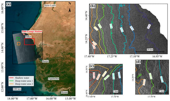
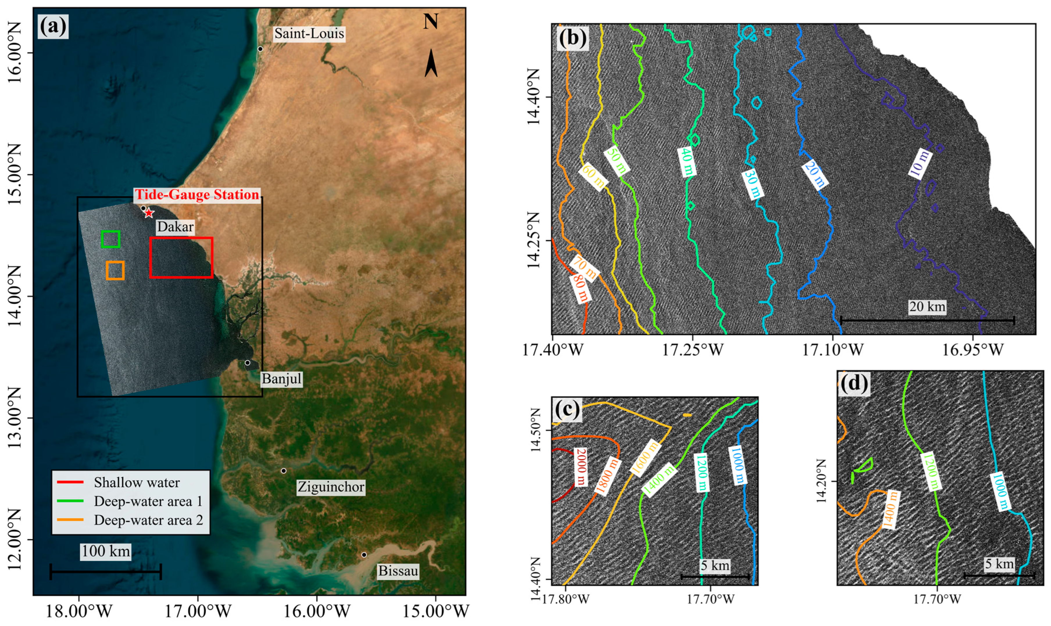
The nearshore waters of Dakar, Senegal, on the west coast of Africa were selected as the study area. The location of the study area and the coverage of the SAR imagery are shown in Figure 1a. Dakar is a major port city in Senegal; the Port of Dakar handles most of the country’s foreign trade and serves as a regional transshipment hub for inland West African countries, giving it a key role in the maritime transport system of Senegal and West Africa [33]. In addition, fisheries along the Senegalese coast are important for employment, coastal livelihoods, and food security [34]. The concentration of socioeconomic activities along the coast also increases the vulnerability of the region to coastal erosion and morphological change [35]. Accurate information on nearshore water depth and its spatial variability is therefore important for navigation safety, fisheries, and coastal-zone management in Dakar.
Figure 1.
Study area and Sentinel-1 SAR imagery. (a) Study-area location, the Dakar tide-gauge station, selected subregions, and the Sentinel-1 image acquired on 20251109 overlaid on the Esri World Imagery basemap; (b) shallow-water area, 20251109; (c) deep-water area 1, 20251109; and (d) deep-water area 2, 20230301. Deep-water area 1 was used for 20230313, 20251109, 20260201, and 20260213, whereas deep-water area 2 was used for 20230301.
The coastal waters off Dakar are exposed to the open Atlantic Ocean and are strongly influenced by swell. Wave hindcast data for 1980–2021 indicate that the Dakar Peninsula is among the more wave-exposed sectors of the Senegalese coast, with a multiyear mean significant wave height of approximately 1.2–1.4 m [36]. The shoreline is generally oriented north–south, and the continental shelf is relatively gentle. The analysis domain spans water depths of approximately 0–80 m (Figure 1b), with isobaths broadly parallel to the coastline and a continuous transition from shallow to intermediate water. This bathymetric setting provides suitable conditions for evaluating retrieval performance across different water-depth ranges. The study area is strongly influenced by offshore swell, and the SAR imagery shows distinct, continuous wave stripes with good local directional consistency. These conditions favor wavelength extraction and bathymetric retrieval based on the linear dispersion relation. In addition, the Dakar tide-gauge station provides tidal information for correcting the water depth to the SAR acquisition time.
2.2. Data Sources
2.2.1. Sentinel-1 Data
Five C-band Sentinel-1 SAR images obtained from the Alaska Satellite Facility Distributed Active Archive Center (ASF DAAC) were used for nearshore wave-stripe identification and bathymetry retrieval. Images acquired on different dates were selected to evaluate the multi-temporal stability of the proposed method. The main image parameters are summarized in Table 1. The VV polarization channel was selected because it provides relatively strong ocean-surface backscatter and clearly captures the bright–dark stripe patterns associated with wave modulation, facilitating wave-stripe identification and local wavelength extraction [7].
Table 1.
Basic information for the Sentinel-1A SAR images.
Because wave stripes in raw SAR imagery may coexist with wind streaks, ship wakes, internal waves, breaking waves, and rain-cell signatures, reliable screening using a single set of quantitative thresholds is difficult. Manual visual inspection was therefore used to assess wave-stripe visibility, continuity, and directional consistency. Only images with sufficiently clear and coherent stripe patterns were retained for subsequent skeleton extraction, directional screening, and wavelength analysis. Clearly identifiable wave stripes are a prerequisite for SAR wave-stripe-based bathymetric retrieval [6].
2.2.2. GEBCO Data
The GEBCO (2026) global terrain dataset was used as the reference bathymetry in this study. The dataset integrates multiple bathymetric sources, including multibeam and single-beam soundings, nautical charts, satellite-gravity-derived estimates, and regional bathymetric products. It is provided on a regular geographic grid at a spatial resolution of 15 arcsec, with depth values expressed in meters. In this study, the GEBCO dataset was used for reference-depth matching, deep-water region selection, and evaluation of bathymetric retrieval accuracy.
2.2.3. Tide Data
Tidal data were used to correct the retrieved water depths for variations in sea level. The tide data were obtained from the tidal information and related services provided by the Service hydrographique et oceanographique de la Marine (SHOM; https://www.shom.fr). The tide-gauge station used in this study is located at Dakar (17.42° W, 14.67° N), as shown in Figure 1. The tidal level at the Sentinel-1 SAR acquisition time was used to ensure vertical-datum consistency between the SAR-derived and reference depths.
2.2.4. Wave Period Data
Wave-period data were obtained from the Copernicus Marine Global Ocean Waves Analysis and Forecast product to independently evaluate the representativeness of the dominant wave period used for bathymetric inversion. Because the SAR-derived wavelength parameters analyzed in this study are associated with long-period swell, the primary-swell mean period (VTM01_SW1) was selected as the main reference period. For SAR images acquired on different dates, the two adjacent 3-hourly wave fields bracketing the image acquisition time were linearly interpolated to the corresponding acquisition time.
2.3. Methodology
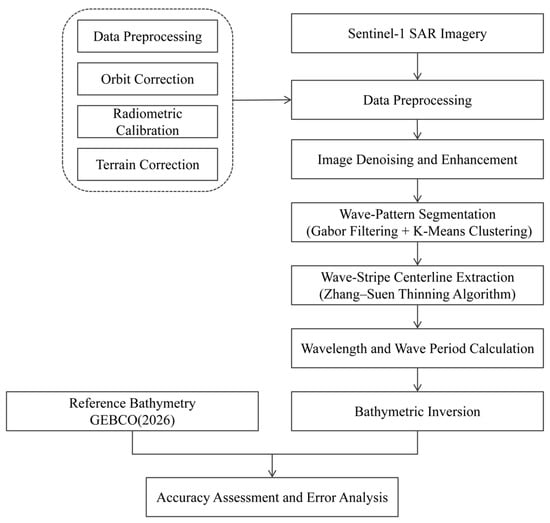
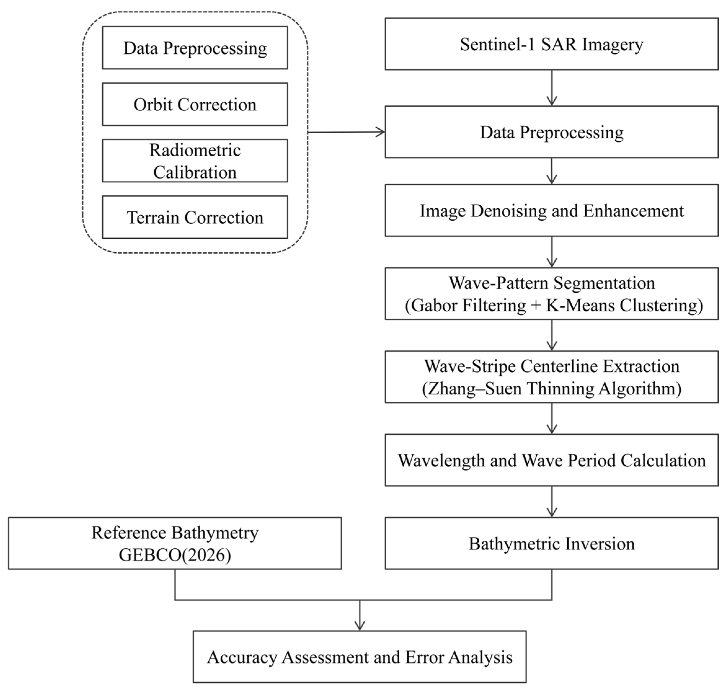
As illustrated in Figure 2, the proposed workflow consists of SAR preprocessing and denoising, wave-stripe extraction and skeleton optimization, wave-period estimation, and bathymetric retrieval using the linear wave dispersion relation.
Figure 2.
Workflow of the proposed method.
2.3.1. Data Preprocessing
The SAR images were first preprocessed using thermal-noise removal, precise orbit correction, radiometric calibration, terrain correction, and study-area clipping. The clipped image was subsequently divided into overlapping subimages, which were used as basic processing units for stripe enhancement, skeleton extraction, and wavelength estimation. Local windowing is widely used for SAR wave-parameter extraction [22,23,24], because it limits the influence of large-scale spatial heterogeneity while preserving locally consistent wave-stripe orientation and wavelength. In this study, sliding windows of 256 × 256 pixels (2.56 km × 2.56 km) were used, with an overlap of 128 pixels (1.28 km) between adjacent windows to reduce the influence of boundary-truncation effects on stripe continuity. The processing window defines only the local image-processing extent and does not represent the spatial resolution of the retrieved bathymetry. Within each window, local wavelength is defined as the normal spacing between adjacent crest lines at a specific location, rather than as a single wavelength representative of the entire 256 × 256-pixel window.
2.3.2. Texture-Preserving TV–Hessian Denoising and Wave-Stripe Enhancement
Clear and continuous wave stripes are essential for reliable extraction of local wavelength and wave-propagation direction from SAR imagery. However, speckle noise can obscure crest–trough patterns, disrupt stripe continuity, and introduce local intensity anomalies, thereby degrading subsequent stripe segmentation and bathymetric retrieval [30,31]. Therefore, denoising should suppress speckle while preserving the structural characteristics of wave stripes.
Following the adaptive total variation bounded Hessian (ATVBH) framework of Cui et al. [32] and the structure-preserving concepts of first- and second-order variational regularization [37], a texture-preserving TV–Hessian denoising model was adopted. Its energy functional is expressed as:
where f is the original noisy SAR image, u is the denoised image, Ω is the image domain, ∇u denotes the first-order gradient term, ∇2u denotes the Hessian-based second-order regularization term, λ is the weight of the data-fidelity term, and κ is the weight of the second-order regularization term. In this study, κ = 0.1. The first-order gradient term helps preserve image edges, whereas Hessian regularization reduces the staircasing artifacts that may occur in conventional total-variation denoising. Together, these terms balance noise suppression and texture preservation [37].
To account for variations in texture intensity among local SAR subimages, the mean gradient energy of the normalized image was calculated as :
where N is the number of pixels and f denotes the normalized SAR image. The data-fidelity weight was then adaptively determined from the image-gradient characteristics:
where λfactor is the fidelity scaling factor, η is the texture-preservation factor, C1 is the reference scale coefficient, and C2 controls the response of the fidelity weight to gradient energy. In this study, λfactor = 8.0, η = 0.9, C1 = 9, and C2 = 50. λmin and λmax define the lower and upper bounds of the fidelity weight, respectively, preventing the adaptive weight from becoming excessively small or large; they were set to λmin = 10−5 and λmax = 2.0. This adaptive strategy enhances structural preservation in strongly textured regions and strengthens denoising in smoother background regions.
After denoising, the local stripe orientation was estimated using the structure tensor, which describes the dominant direction of image texture through the covariance of local gradients [38]:
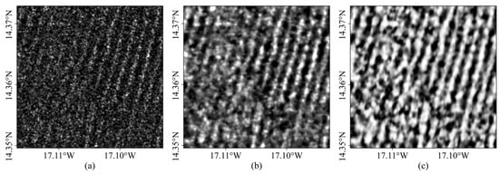
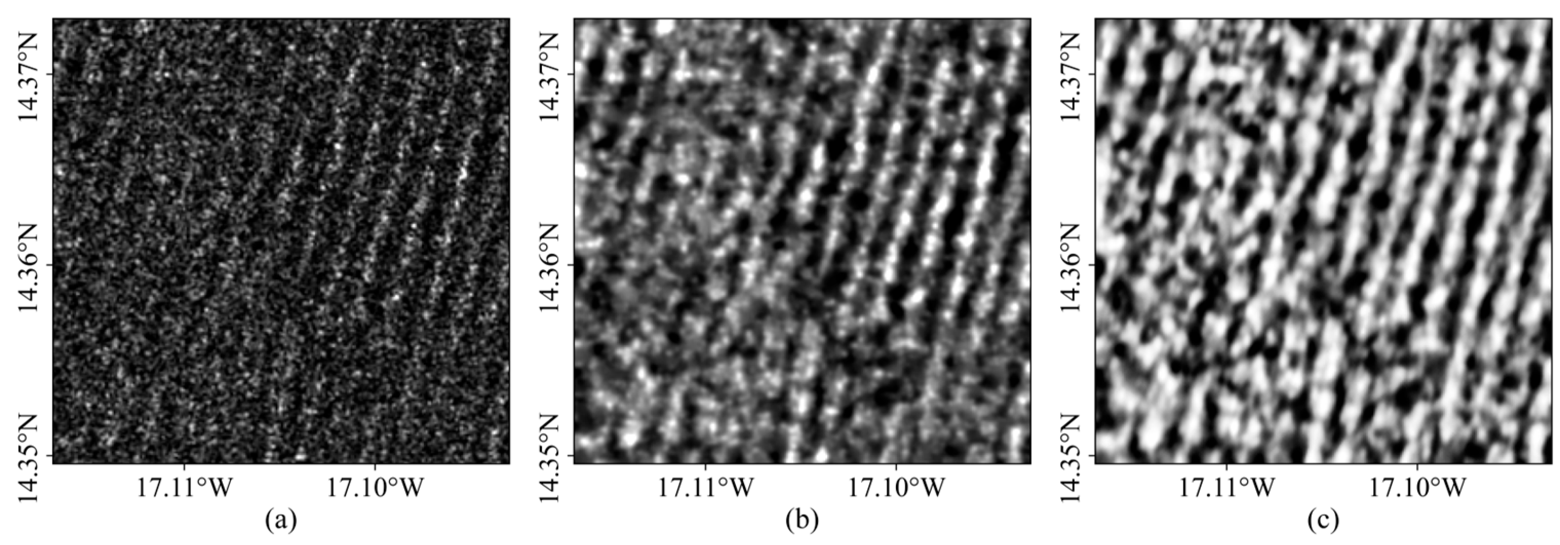
where ux and uy are the horizontal and vertical image gradients, respectively, and Kρ denotes a Gaussian smoothing kernel. The dominant orientation derived from the structure tensor was subsequently used to guide directional smoothing and enhancement along the wave stripes. This operation reconnects locally fragmented stripe features while limiting smoothing across crest–trough boundaries. As shown in Figure 3, the combined denoising and directional enhancement improve stripe continuity and local contrast, providing a more reliable basis for subsequent stripe segmentation and wavelength extraction.
Figure 3.
Comparison before and after denoising. (a) Original image; (b) denoised image; (c) denoised and enhanced image.
2.3.3. Wave-Stripe Segmentation Using Gabor Filtering and K-Means Clustering
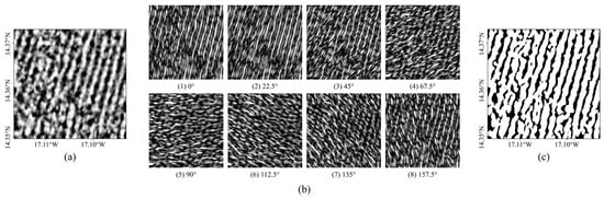
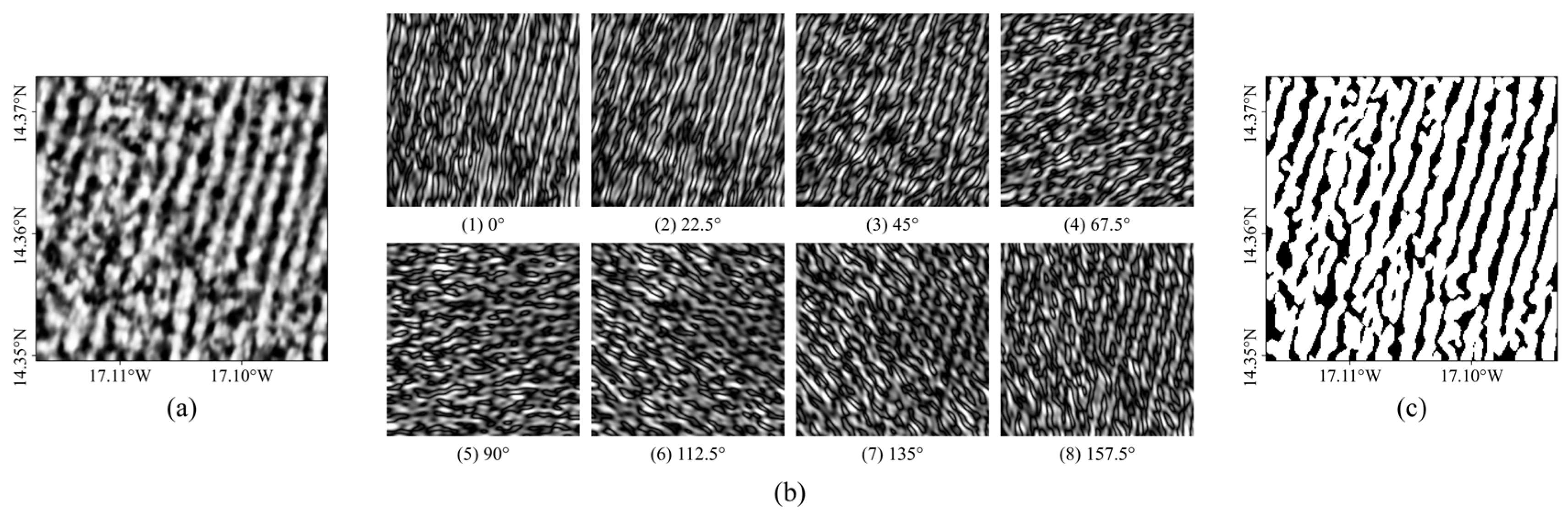
Wave stripes in SAR images usually appear as periodic textures with distinct directional and spatial-frequency characteristics. Gabor filters characterize local orientation and spatial-frequency information while providing localization in both the spatial and frequency domains [39,40]. Previous studies have successfully combined Gabor filtering with K-means clustering for internal-wave stripe segmentation in SAR imagery [41]. A multidirectional Gabor filter bank was applied to the denoised and enhanced image to extract wave-texture responses across different orientations. Figure 4a and Figure 4b show the denoised and enhanced image and its eight-direction Gabor-filter responses, respectively.
Figure 4.
Gabor filtering and K-means clustering segmentation. (a) Denoised and enhanced image; (b) eight-direction Gabor-filter responses; (c) segmentation result of the bright-stripe class.
The two-dimensional Gabor filter is defined as:
where xθ and yθ are the coordinates after rotation by the filtering direction θ, with xθ = xcosθ + ysinθ and yθ = −xsinθ + ycosθ, λg is the filter wavelength, σ is the standard deviation of the Gaussian envelope, γ is the spatial aspect ratio, and ψ is the phase offset. To accommodate different local wave directions, an eight-direction Gabor filter bank was used:
The enhanced SAR image was convolved with each directional Gabor kernel to obtain multidirectional response features. For each pixel, the feature vector can be expressed as:
where Rm(x,y) is the Gabor response in the m-th direction. These multidirectional features enhance wave stripes with specific orientations and periodicities while suppressing isotropic speckle noise and nonperiodic background textures.
Because stripe contrast varies among subimages, a fixed threshold may not provide robust segmentation across the entire scene. K-means clustering was therefore applied to the multidirectional Gabor-response features to partition the pixels into bright-stripe and background regions (Figure 4c). K-means is a common unsupervised clustering method that partitions samples by minimizing within-cluster distance [42]. The clustering objective is:
where Si denotes the set of pixels assigned to cluster i, F(x) is the multidirectional Gabor-response feature vector of pixel x, and μi is the corresponding cluster center. Here, k = 2, corresponding to the bright-stripe and background classes. The class with the higher mean gray level was identified as the bright-stripe class:
where Ie(i) is the gray value of the i-th pixel after denoising, enhancement, and normalization, and c* is the final bright-stripe class. A binary image of bright stripes was then obtained.
To improve stripe continuity, morphological closing was applied to connect fragmented stripe regions, followed by connected-component filtering to remove small spurious features [43].
2.3.4. Wave-Crest Skeleton Extraction and Optimization
- (1)
- Wave-Crest Skeleton Extraction
The Zhang–Suen thinning algorithm is a classical skeletonization method that iteratively removes boundary pixels from binary objects while preserving their connectivity and topology, thereby reducing stripe-like regions to single-pixel-wide skeletons [44]. In this study, the Zhang–Suen thinning algorithm was applied to the segmented bright wave stripes to extract single-pixel-wide wave-crest skeletons. This step reduces the influence of stripe width while preserving the orientation and continuity of the wave crests. The resulting skeletons provide a stable geometric basis for crest matching and local wavelength measurement.
- (2)
- Skeleton Optimization
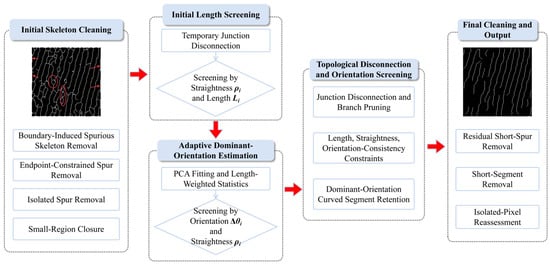
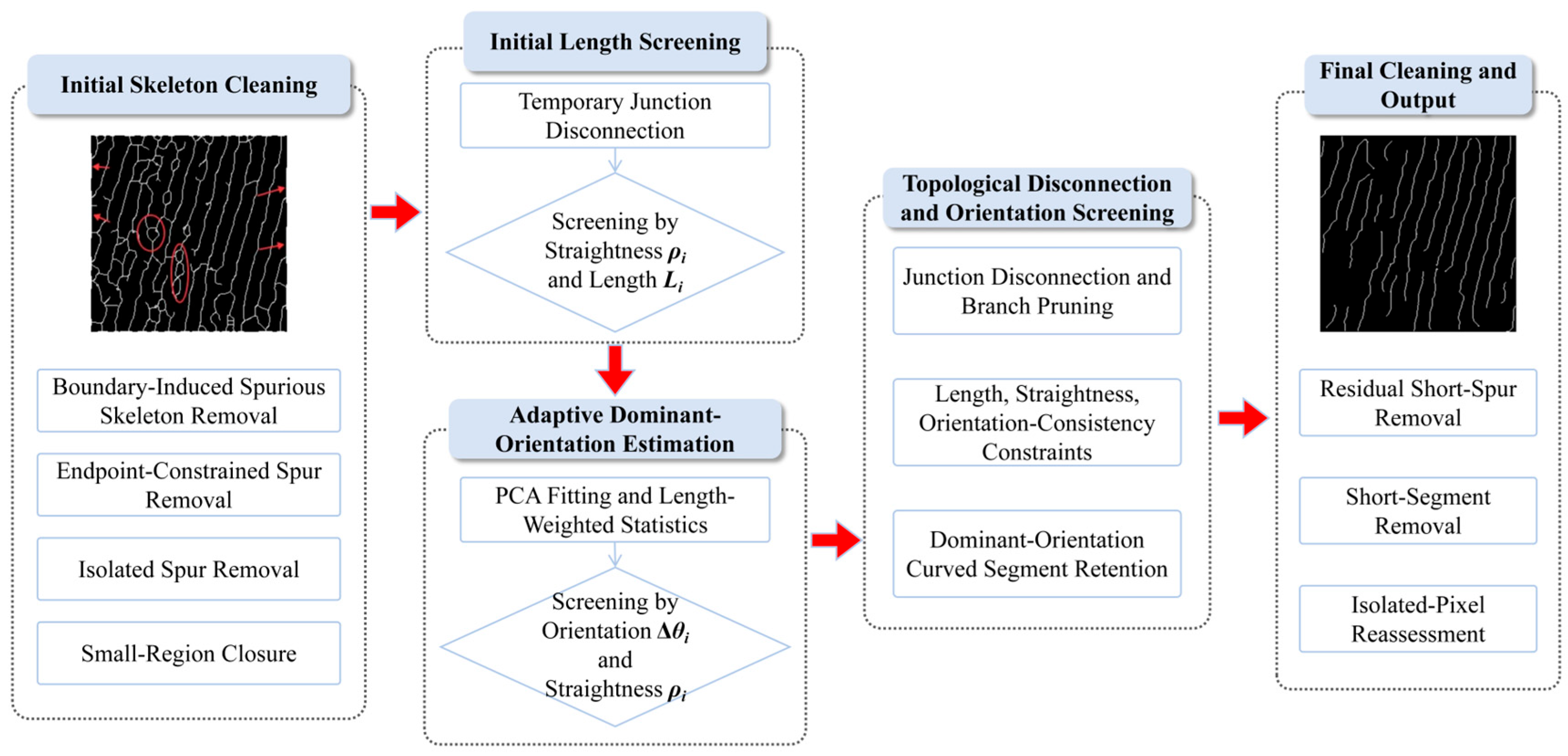
Residual noise and local deformation of wave stripes may introduce short spurs, false branches, intersections, and irregularly curved segments into the skeletons obtained by Zhang–Suen thinning. Because these artifacts can interfere with subsequent wavelength measurement, further skeleton pruning and topological optimization are required [45,46]. Therefore, the initial skeletons were further optimized based on morphological characteristics and directional consistency, as illustrated in Figure 5.
Figure 5.
Workflow of wave-crest skeleton optimization. Red arrows indicate the processing sequence.
Junction pixels were first temporarily removed to decompose the connected skeleton into individual branches. For each branch, the length Li was calculated from the number of skeleton pixels, and straightness ρi was defined as the ratio of the Euclidean distance between two representative extreme points to the branch length:
Values of ρi approaching 1 indicate a nearly straight branch. The orientation of each branch was estimated from the first principal component of its pixel coordinates using PCA. The dominant wave-stripe orientation was then estimated from sufficiently long and straight branches using length-weighted axial averaging. The angular deviation Δθi between each branch and the dominant wave-stripe orientation was then calculated by accounting for the 180° axial symmetry of stripe orientation. A branch was retained when it simultaneously satisfied:
where Li is the branch length in pixels, ρi is the branch straightness, and Δθi is the axial angular deviation from the dominant wave-stripe orientation. These empirical thresholds were selected to preserve skeleton continuity and directional consistency while maintaining a sufficient number of wavelength samples, rather than being retrospectively tuned to maximize bathymetric accuracy. To avoid removing genuine wave-crest segments with moderate curvature, local PCA was additionally applied to retain segments whose orientations remained locally consistent with the dominant wave-stripe orientation. Finally, residual short spurs, short connected components, and isolated pixels were removed to obtain the optimized wave-crest skeleton.
Li ≥ 15, ρi ≥ 0.80, Δθi ≤ 15°
2.3.5. Physical Model for Bathymetry Retrieval
- (1)
- Wavelength Calculation and Outlier Rejection
To reduce the effects of residual noise, fragmented skeletons, and irregular wave stripes on wavelength estimation, a two-level quality-control procedure was applied to the candidate wavelength measurements. Previous studies have incorporated quality-control procedures into wave-parameter extraction and bathymetric inversion [47].
At the first level of quality control, each subimage was first evaluated based on the number of skeleton pixels, number of connected branches, branch length, and directional consistency. For each retained subimage, 200 parallel sampling lines were then placed normal to the dominant skeleton orientation. Candidate local wavelengths were measured from the spacing between adjacent crest lines along each sampling line. A sliding-window search was used to identify the dominant wavelength band containing the largest number of samples. The window width was set to 15% of the median candidate spacing, and the preliminary valid interval was defined as ±12% of the central value of the dominant band. The effective-wavelength ratio Rv and coefficient of variation CV were then calculated:
where Nvalid is the number of effective samples within the dominant wavelength band, Ntotal is the total number of candidate wavelengths, and the mean and standard deviation of the wavelength samples are denoted by μλ and σλ, respectively. When Rv < 0.30 and CV > 0.25, the wavelength distribution was considered insufficiently regular, and the corresponding subimage was excluded from further analysis.
At the second level, 200 equally spaced sampling lines were placed normal to the dominant wave-crest orientation in each retained subimage, with a 2-pixel interval between adjacent sampling lines. The intersection points between each sampling line and the crest lines were identified as crest points, and the distance between adjacent crest points was taken as the local wavelength:
To suppress unrealistic wavelength estimates caused by skeleton breaks, incorrect crest matching, and residual noise, the candidate wavelengths were filtered using the median absolute deviation (MAD). Samples outside the range of median (λ) ± 3MAD were removed. The dominant wavelength band was then identified using a sliding-window search, and only wavelengths within a prescribed relative deviation from the center of the dominant band were retained as effective wavelengths. This two-step filtering procedure reduces the influence of incorrect crest matching and non-target textures on local wavelength estimation, thereby providing reliable wavelength samples for subsequent dominant-period estimation and bathymetric inversion.
- (2)
- Wave-Period Estimation and Bathymetry Retrieval Based on the Linear Dispersion Relation
According to linear wave theory, the wave period T remains approximately constant as swell propagates from deep to shallow water, whereas the wavelength L decreases as the water depth h decreases. Water depth can therefore be retrieved from the local wavelength and a representative wave period using the linear wave dispersion relation:
where ω is the angular frequency, k is the wave number, g is gravitational acceleration, ω = 2π/T, and k = 2π/L.
ω2 = gktanh(kh)
Because local wavelength can be extracted directly from SAR imagery whereas wave period cannot, a representative period was estimated from the deep-water wavelength. Under the deep-water condition h > L/2, bottom effects are negligible and the dispersion relation can be approximated as ω2 = gk, giving the following:
where L0 is the representative deep-water wavelength. The deep-water regions shown in Figure 1c,d were selected based on the GEBCO reference bathymetry, where water depths exceed approximately 600 m and satisfy the deep-water condition. For the image acquired on 20230301, the region shown in Figure 1d was used instead of the region in Figure 1c because an anomalously dark area was present at the same location, making the wave stripes difficult to identify reliably. Effective wavelengths extracted from this region using the preceding skeleton-based method were mainly distributed between 280 and 440 m. The wavelength corresponding to the peak of the kernel density estimate was taken as L0 and used to determine the representative wave period T. The water depth h can then be expressed as:
Water depth was subsequently retrieved for each effective wavelength sample. Because the SAR-derived bathymetric samples are spatially discrete and densely distributed, the retrievals were spatially matched to the minimum GEBCO grid cells for comparison with the GEBCO reference depths. Therefore, the final bathymetric accuracy assessment was performed at the GEBCO grid resolution rather than at the scale of the original wavelength samples or processing windows.
3. Results
3.1. Wave-Crest Skeleton Extraction Results
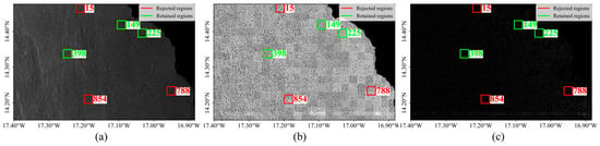
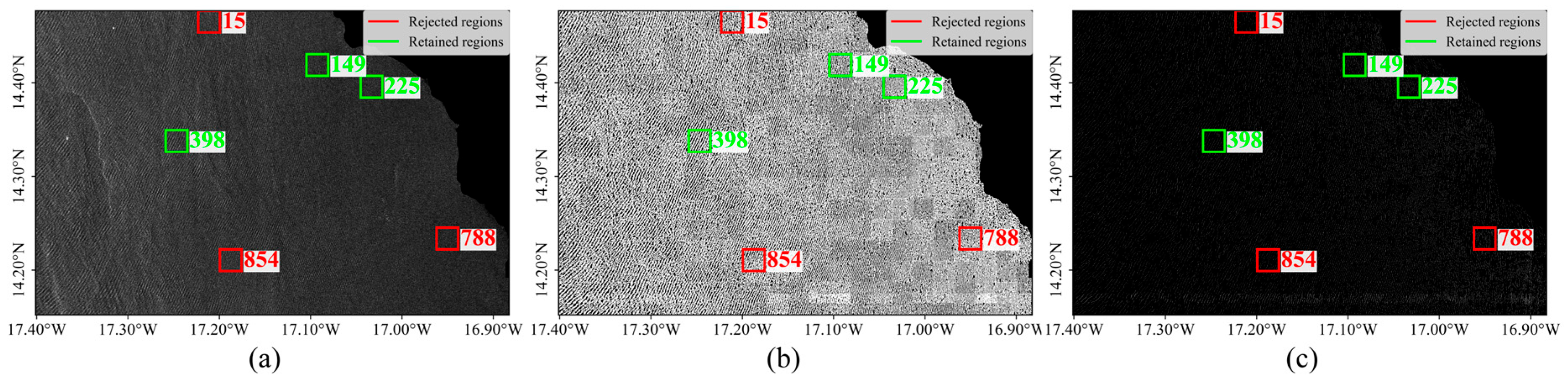
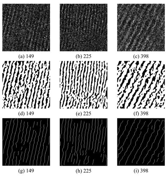
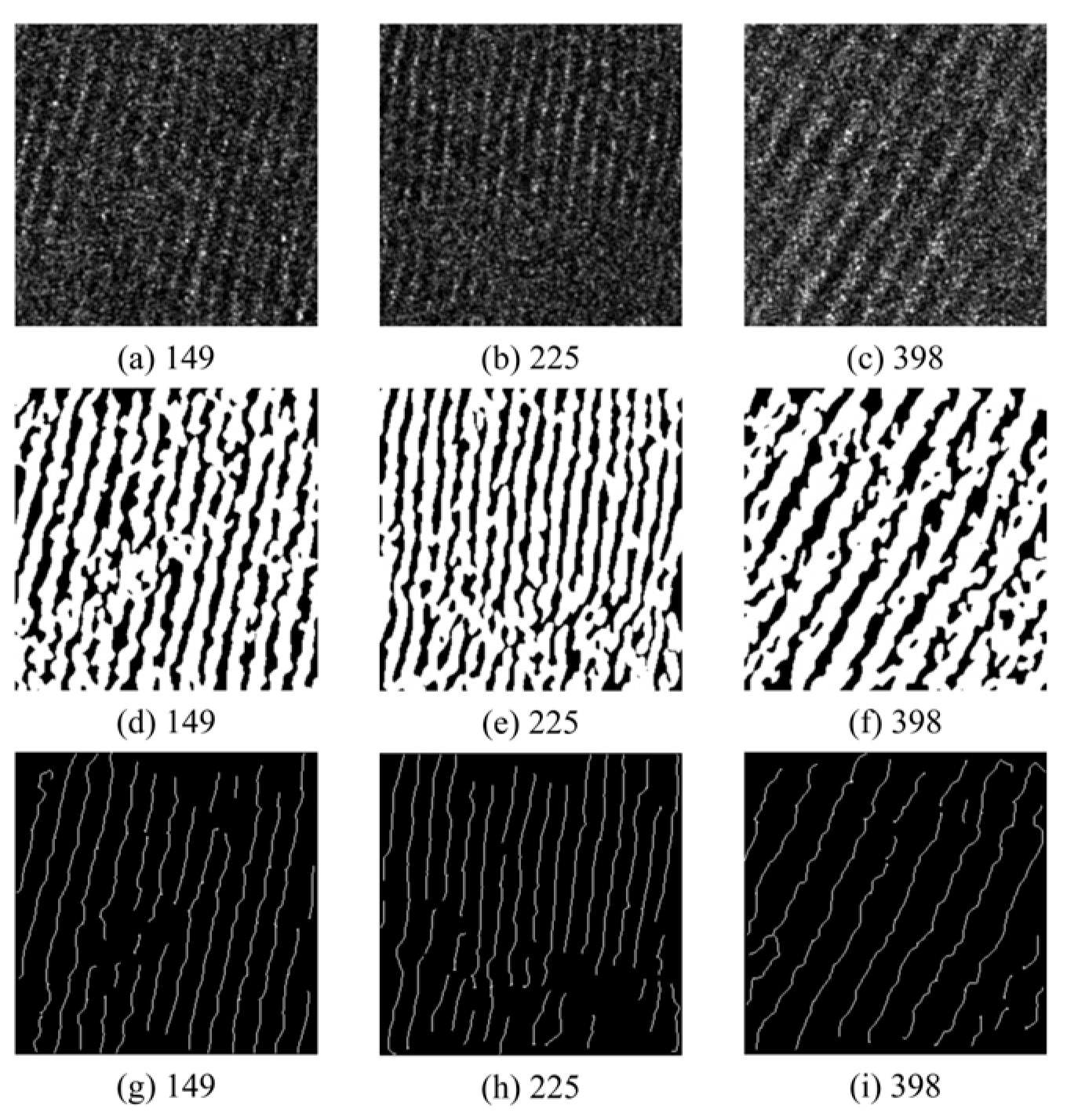
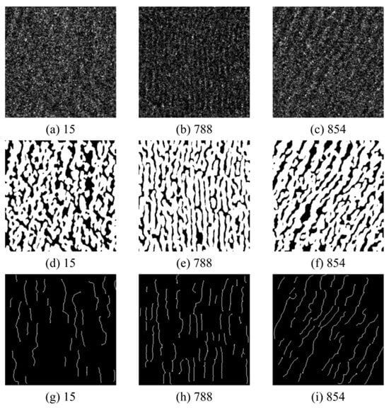
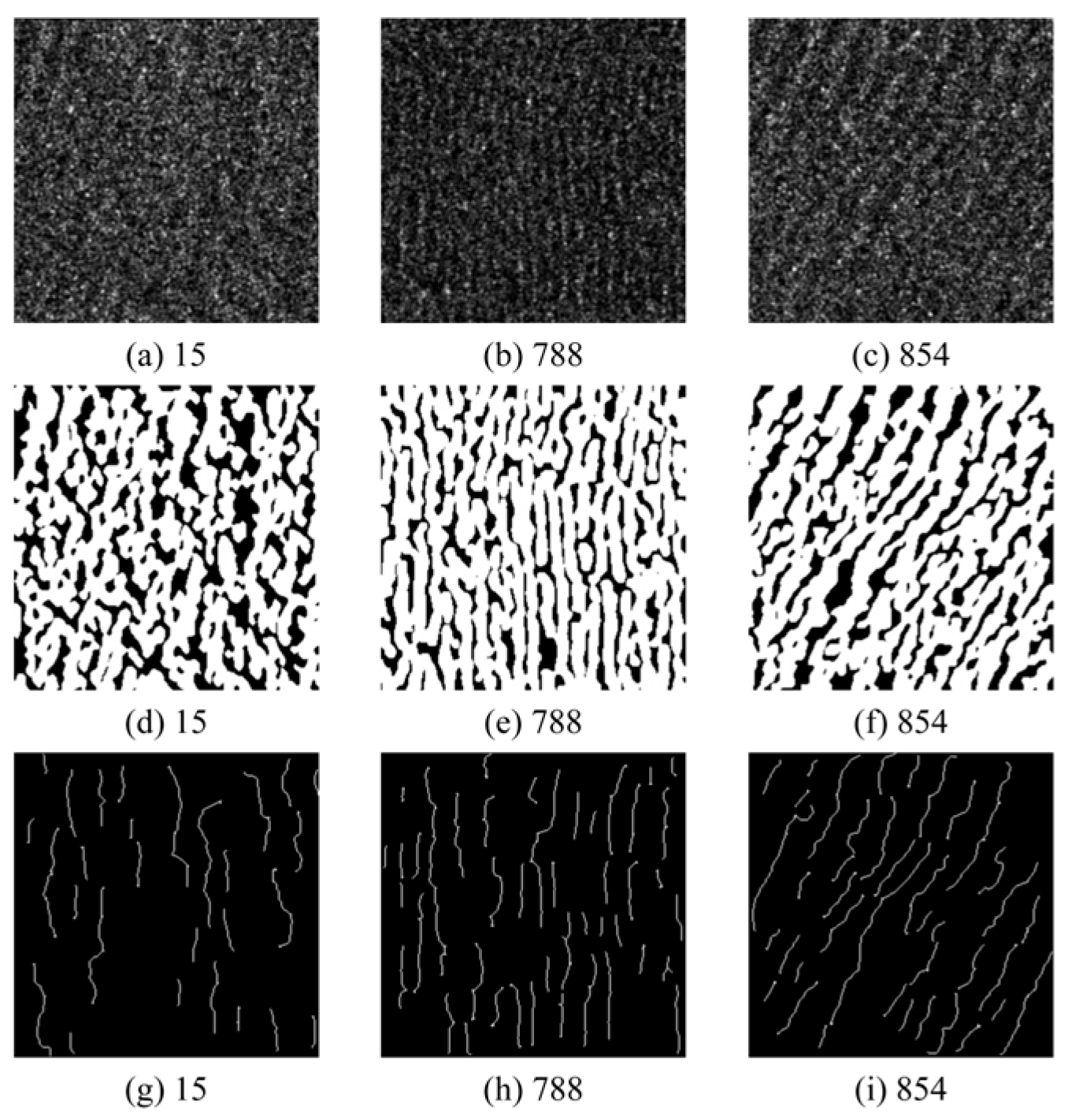
Figure 6 presents the wave-stripe extraction and quality-screening results for the 20251109 SAR image as a representative example. Compared with the original SAR image (Figure 6a), Figure 6b,c demonstrate that the principal wave stripes were successfully extracted and that subimages could be screened according to stripe integrity and skeleton quality. To evaluate extraction performance under different stripe-quality conditions, three retained subimages (Figure 7) and three rejected subimages (Figure 8) were selected for detailed comparison. Green boxes indicate subimages that passed the quality screening and were retained for wavelength extraction, whereas red boxes indicate rejected subimages. The numbers beside the boxes indicate the IDs of the corresponding subimages used for the detailed comparisons in Figure 7 and Figure 8.
Figure 6.
Crest-line extraction results (20251109). (a) Original image; (b) segmented bright stripes; (c) extracted wave-crest skeletons.
Figure 7.
Local extraction results for green-boxed retained stripe regions (20251109). (a–c) Original images; (d–f) segmented bright stripes; (g–i) extracted wave-crest skeletons.
Figure 8.
Local extraction results for red-boxed rejected stripe regions (20251109). (a–c) Original images; (d–f) segmented bright stripes; (g–i) extracted wave-crest skeletons.
As shown in Figure 7, the retained regions exhibit well-defined alternating bright and dark wave stripes, with generally consistent orientations and good continuity. After segmentation, the principal bright wave stripes remain continuous and well defined. Subsequent skeletonization produces single-pixel-wide crest lines distributed near the centers of the bright stripes, with relatively stable spacing between adjacent crest lines. In contrast, the rejected regions in Figure 8 exhibit more pronounced local discontinuities and directional variations, with some areas containing fragmented linear or patch-like structures. Their skeletons are correspondingly fragmented and directionally inconsistent, making reliable crest matching and local wavelength measurement difficult. The quality-screening procedure therefore retains only subimages that provide reliable wave-crest lines for subsequent wavelength estimation.
3.2. Wave-Parameter Extraction Results
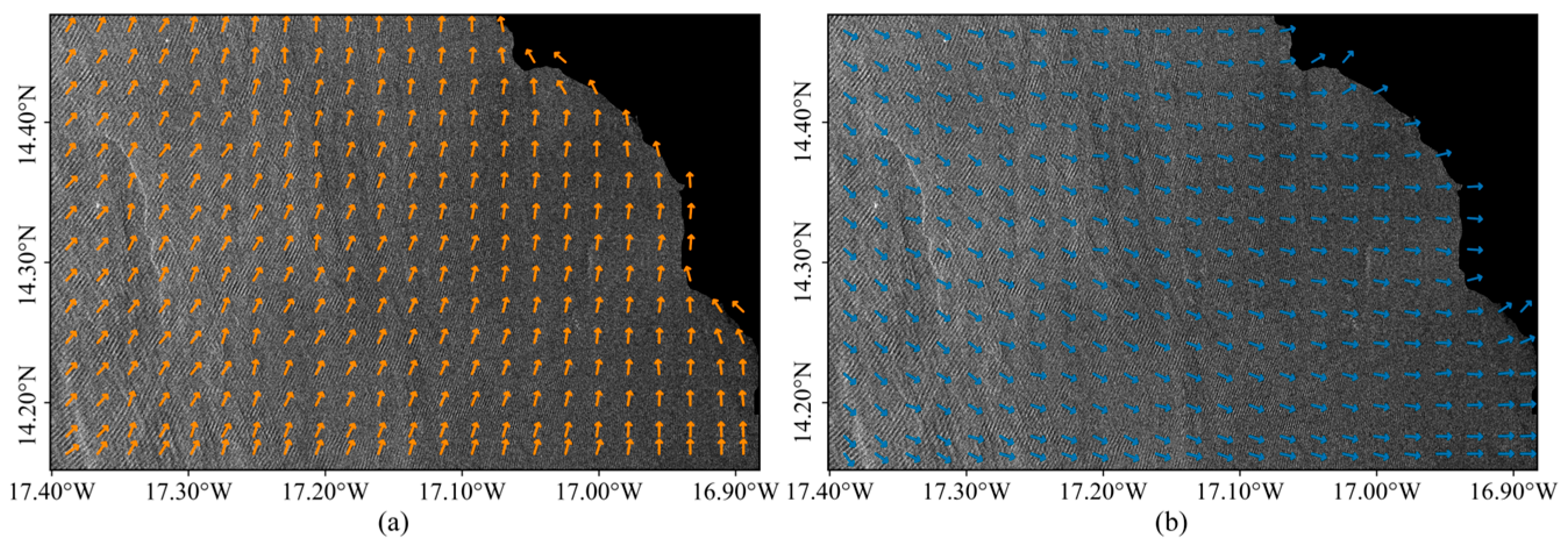
Wave-stripe orientation was first derived from the extracted wave-crest skeletons. The corresponding crest-normal direction was then combined with the coastline position to determine the shoreward wave-propagation direction. Figure 9 shows the spatial distributions of wave-stripe orientation and wave-propagation direction for the 20251109 SAR image. The two fields are approximately perpendicular and exhibit smooth spatial variations. Near the coast, the wave-propagation direction shows some local turning, which may be associated with wave refraction induced by water-depth variations and shoreline geometry.
Figure 9.
Wave-stripe orientation and wave-propagation direction (20251109). (a) Wave-stripe orientation (indicated by orange arrows); (b) wave-propagation direction (indicated by blue arrows).
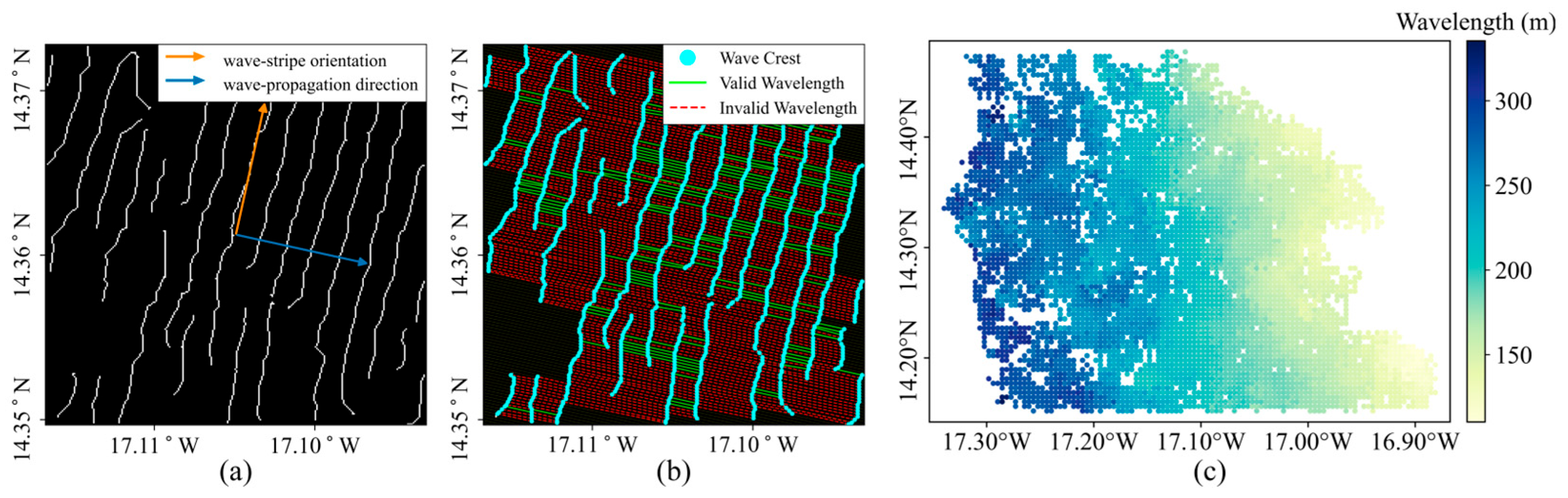
Sampling lines were oriented along the wave-propagation direction, and the local wavelength was calculated as the normal spacing between adjacent wave-crest lines. Figure 10 shows the relationship between wave-stripe orientation and propagation direction, crest-point identification, and effective-wavelength screening for the 20251109 SAR image. After range screening and outlier removal, the extracted wavelengths exhibited a clear spatial gradient. Longer wavelengths occurred mainly in the northwestern offshore area, whereas shorter wavelengths were concentrated in the southeastern nearshore area, indicating progressive wavelength shortening toward the coast. This pattern is consistent with the expected wavelength decrease as waves propagate into shallower water. Local wavelength variability and data gaps were also observed, particularly near approximately 17.2° W, 14.45° N in the northern part of the study area, 17.27° W, 14.24° N in the southwest, and 16.95° W, 14.27° N in the southeast. These spatial discontinuities indicate regional differences in wave-stripe detectability and in the number of effective wavelength samples available for retrieval.
Figure 10.
Local wavelength extraction and spatial distribution (20251109). (a) Local wave-stripe orientation and wave-propagation direction in a subimage; (b) wavelength extraction along crest-line normals and outlier filtering; (c) spatial distribution of wavelengths.
Table 2 further compares the wavelength-extraction support scales reported in related SAR wave-based bathymetric studies. Previous approaches have mainly relied on window-based spectral methods, such as FFT or wavelet analysis. In the proposed method, by contrast, subimages serve only as local processing units, while local wavelengths are measured directly from the normal spacing between adjacent wave-crest lines. This direct spatial-domain measurement reduces the window-scale averaging of local wavelength variability.
Table 2.
Comparison of wavelength extraction support scales in previous SAR wave-based bathymetric studies.
3.3. Bathymetric Retrieval and Spatial Error Distribution
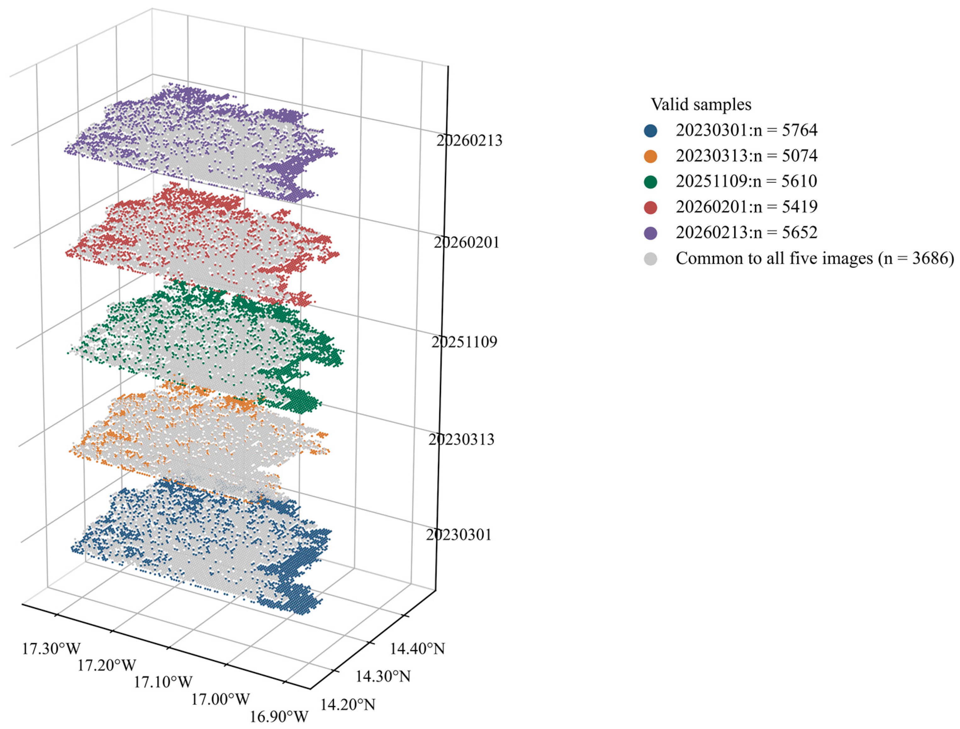
To ensure spatial comparability among the multi-temporal retrievals, only locations with valid bathymetric estimates in all five SAR acquisitions were retained. As shown in Figure 11, a three-dimensional layered display was used to illustrate the spatial distributions of valid bathymetric samples from different acquisition dates. The spatial coverage of valid samples varied among the five acquisition dates, while 3686 locations were common to all five scenes. The retrieved depths at these common locations were then averaged across the five acquisition dates to evaluate the multi-temporal robustness of the method.
Figure 11.
Spatial distribution of valid bathymetric samples for the five Sentinel-1 acquisitions.
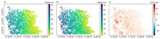
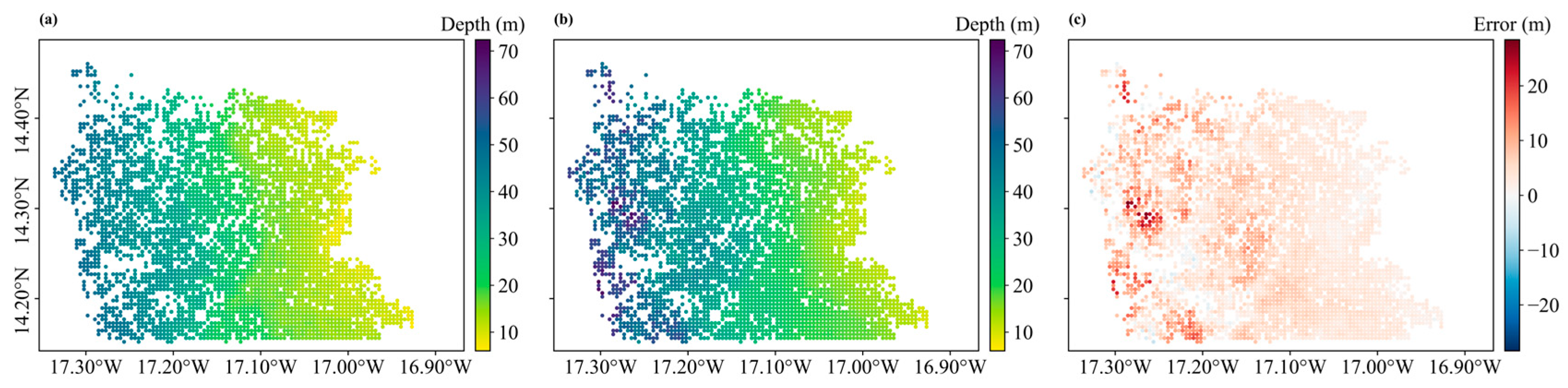
Figure 12 compares the resulting multi-temporal mean retrieved depths with the corresponding GEBCO reference depths at the same locations. Both the GEBCO bathymetry (Figure 12a) and the multi-temporal mean SAR-derived bathymetry (Figure 12b) exhibit a consistent offshore-deepening pattern, with water depth increasing from the southeastern nearshore zone (approximately 16.9° W–17.1° W) toward the northwestern offshore zone (approximately 17.2° W–17.3° W). The multi-temporal mean retrieved bathymetry reproduces the overall spatial depth pattern of the GEBCO reference, with relatively smooth spatial variations across most of the common retrieval area. As shown in Figure 12c, where the error is defined as retrieved depth minus GEBCO depth, the error distribution is predominantly positive, indicating an overall tendency toward depth overestimation. Larger positive deviations are mainly concentrated in the deeper northwestern sector near 17.2° W and in several localized areas with pronounced depth variations, whereas negative deviations are relatively sparse. Overall, the multi-temporal mean SAR-derived bathymetry reproduces the principal nearshore-to-offshore bathymetric gradient of the GEBCO reference, although larger discrepancies remain primarily in deeper water.
Figure 12.
Spatial distribution of water depth. (a) GEBCO bathymetry; (b) multi-temporal mean SAR-derived bathymetry; (c) retrieval error.
3.4. Bathymetric Retrieval Accuracy
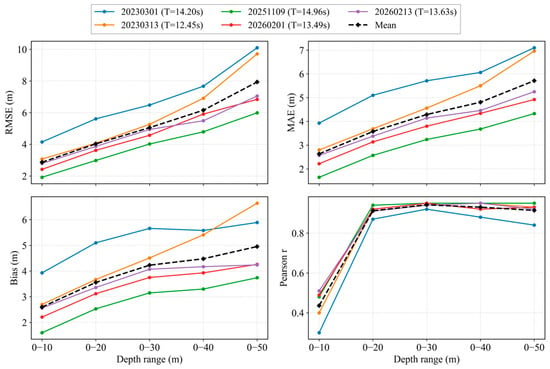
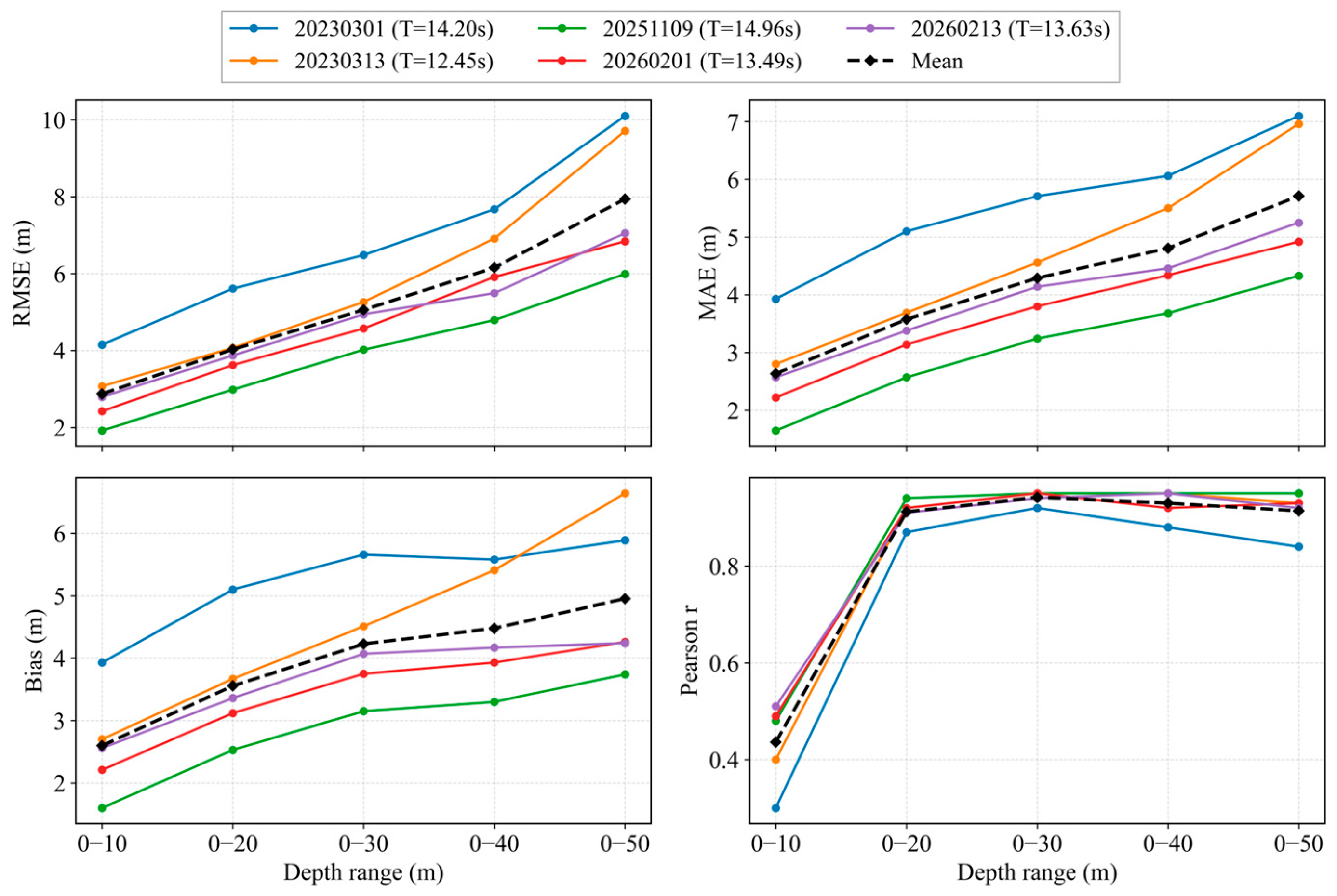
To evaluate the applicability of the proposed method under different SAR imaging conditions, only the common spatial locations with valid bathymetric retrievals in all five acquisitions were used for comparison. As shown in Figure 13, RMSE, MAE, and Bias generally increase as the cumulative depth range expands, whereas the correlation coefficient remains high over most depth ranges. Based on the mean statistics across the five acquisitions, the cumulative 0–20 m range yields an RMSE of approximately 3.87 m, an MAE of 3.56 m, and a correlation coefficient of 0.95. When the depth range is extended to 0–50 m, the RMSE increases to approximately 6.06 m, while the correlation coefficient remains high at 0.97. Although some differences in retrieval accuracy occur among individual acquisition dates, the overall depth-dependent trends are highly consistent, indicating that the proposed method can be reliably applied to multi-temporal Sentinel-1 imagery and can reproduce the general nearshore-to-offshore deepening pattern of the study area.
Figure 13.
Multi-temporal bathymetric retrieval accuracy of the five SAR images over cumulative depth ranges.
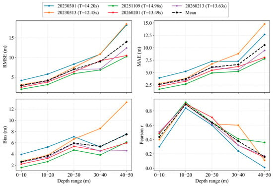
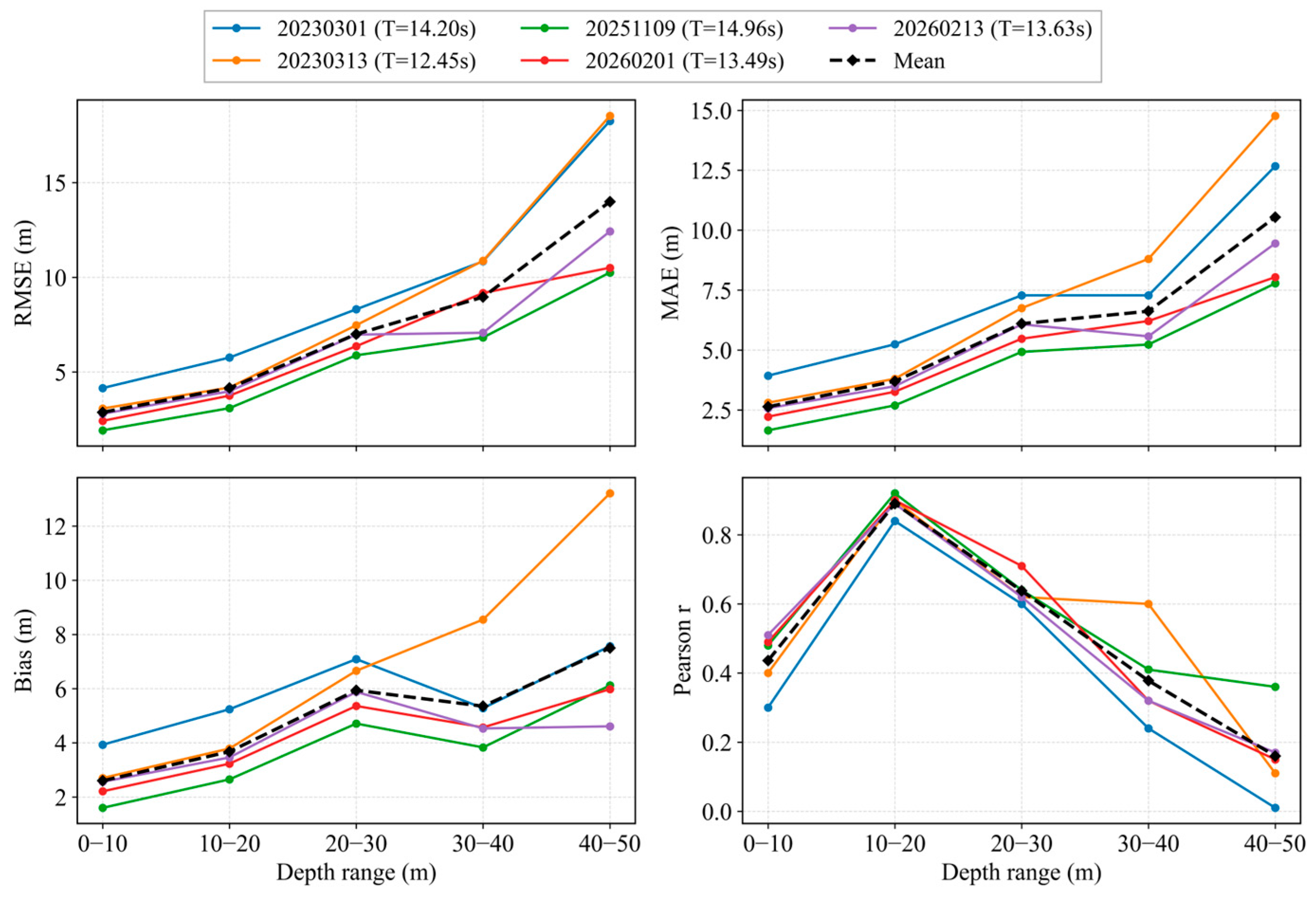
Figure 14 further illustrates the multi-temporal retrieval accuracy within independent depth intervals. All five acquisitions exhibit a common pattern of relatively low errors in shallow water and progressively increasing errors with depth. It should be noted that no common valid samples shallower than 5 m were available across the five acquisitions; therefore, the nominal 0–10 m interval effectively represents water depths of approximately 5–10 m. Considering all five acquisitions, the 10–20 m interval shows the strongest correlations together with relatively low errors, with r ranging from approximately 0.84 to 0.92. Bias values are positive across all depth intervals and generally increase with depth, indicating an overall tendency toward depth overestimation. However, the variation in Bias does not fully coincide with that of RMSE, which may be partly attributed to the cancellation of positive and negative errors within the same depth interval. For example, in the 30–40 m interval, Bias decreases slightly relative to the 20–30 m interval for all acquisition dates except 20230313, whereas RMSE generally increases with increasing water depth. Overall, both RMSE and MAE become markedly larger in the 30–50 m range, with RMSE reaching approximately 10–19 m in the 40–50 m interval. Considering both absolute errors and correlation, the method therefore exhibits its most stable performance within the 5–20 m depth range.
Figure 14.
Multi-temporal bathymetric retrieval accuracy of the five SAR images within independent depth intervals.
In addition, averaging the retrieved depths at the common spatial locations across the five acquisition dates reduces the influence of scene-specific wave conditions, image-texture variability, and anomalous retrievals, thereby providing a more stable bathymetric estimate. The multi-temporal mean bathymetry shows good spatial agreement with the GEBCO reference bathymetry and provides a more representative estimate of the overall mean bathymetric pattern of the study area.
4. Discussion
4.1. Influence of Dominant-Wave-Period Selection
Uncertainty in the wave period propagates into bathymetric retrieval through the linear dispersion relation, and its influence generally increases with water depth [15,18,19].
To assess their representativeness independently, the SAR-derived wave periods were compared with the CMEMS primary-swell mean period (VTM01_SW1) over the retrieval area. As summarized in Table 3, the SAR-derived periods range from 12.45 to 14.96 s, while the corresponding CMEMS periods range from 11.40 to 13.53 s. The SAR-derived periods are consistently 0.90–2.08 s higher than the CMEMS values, with a mean difference of 1.43 s. This systematic difference is reasonable because the SAR-derived value represents a dominant period inferred from wave-crest spacing, whereas VTM01_SW1 represents the spectral-moment mean period of the primary-swell partition. Overall, the two datasets are comparable in magnitude and exhibit similar temporal variations, supporting the use of the SAR-derived period as a representative wave period for bathymetric inversion.
Table 3.
Comparison between the SAR-derived dominant wave periods and the CMEMS primary-swell mean periods (VTM01_SW1).
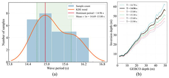
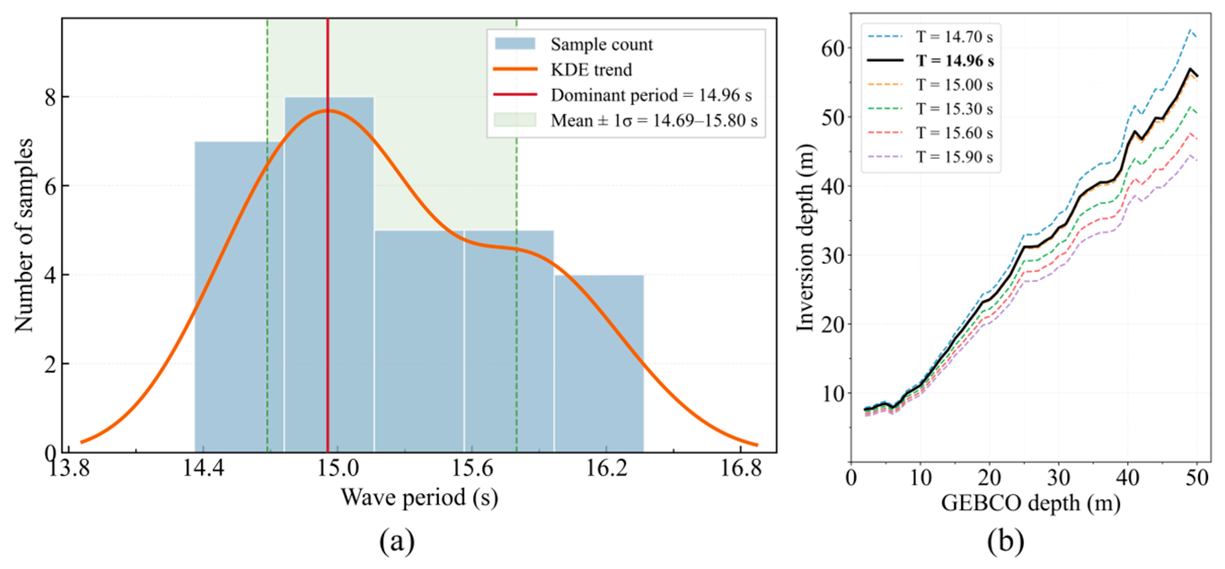
Based on the kernel density estimate of the effective deep-water wavelengths for 20251109, the dominant wave period was determined as 14.96 s. A sensitivity analysis was then conducted over the range defined by the mean wave period plus or minus one standard deviation (1σ). The lower and upper bounds were rounded to one decimal place, and wave-period scenarios were selected at 0.3 s intervals within this range (Figure 15). The results show that shorter periods produce systematically greater retrieved depths, whereas longer periods yield shallower estimates. This effect is relatively limited in shallow water but becomes more pronounced in deeper areas. As water depth increases, tanh(kh) approaches unity, reducing the sensitivity of the dispersion relation to depth and amplifying the effect of period uncertainty on the retrieved bathymetry.
Figure 15.
Determination of the dominant wave period based on kernel density estimation (20251109). (a) Dominant wave-period determination; (b) depths calculated using different periods.
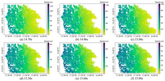
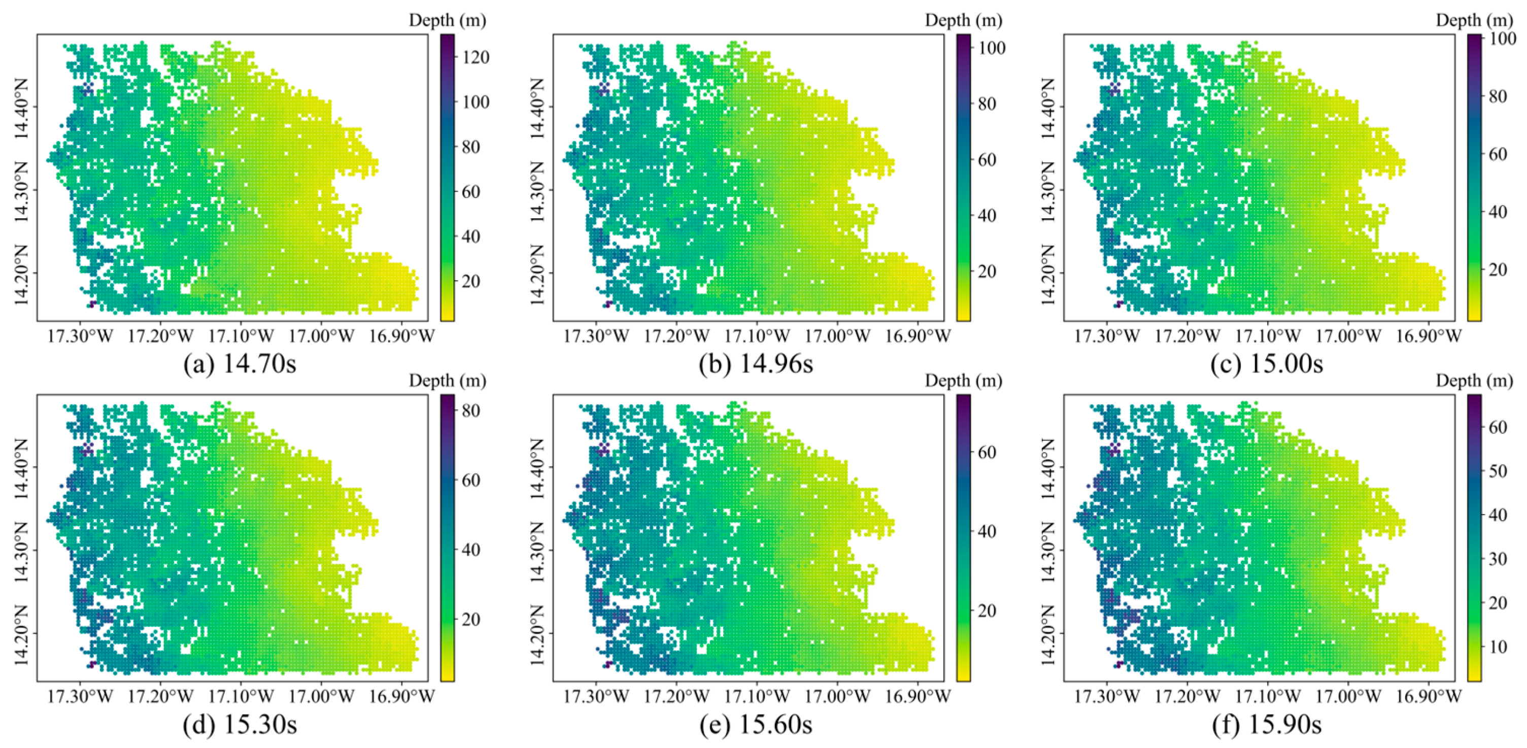
The overall spatial pattern of the retrieved bathymetry remains similar among the different period scenarios, whereas the absolute depth and systematic bias vary substantially (Figure 16 and Table 4). As the period increases from 14.70 to 15.90 s, the Bias decreases from 5.42 m to −1.13 m, while the RMSE decreases from 7.99 m to a minimum of 3.59 m at 15.60 s before increasing slightly to 3.84 m at 15.90 s. In contrast, the correlation coefficient remains within 0.95–0.96 across all scenarios. These results indicate that dominant-period selection has limited influence on the overall spatial pattern of the retrieved bathymetry but substantially affects absolute depth and systematic bias, particularly in deeper water.
Figure 16.
Spatial bathymetric variation under different periods (20251109).
Table 4.
Error metrics for bathymetric retrieval under different dominant periods for 20251109 (0–50 m).
4.2. Influence of Wave-Crest Skeleton Positioning Error
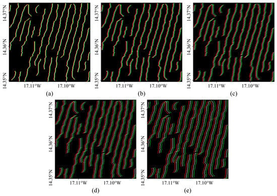
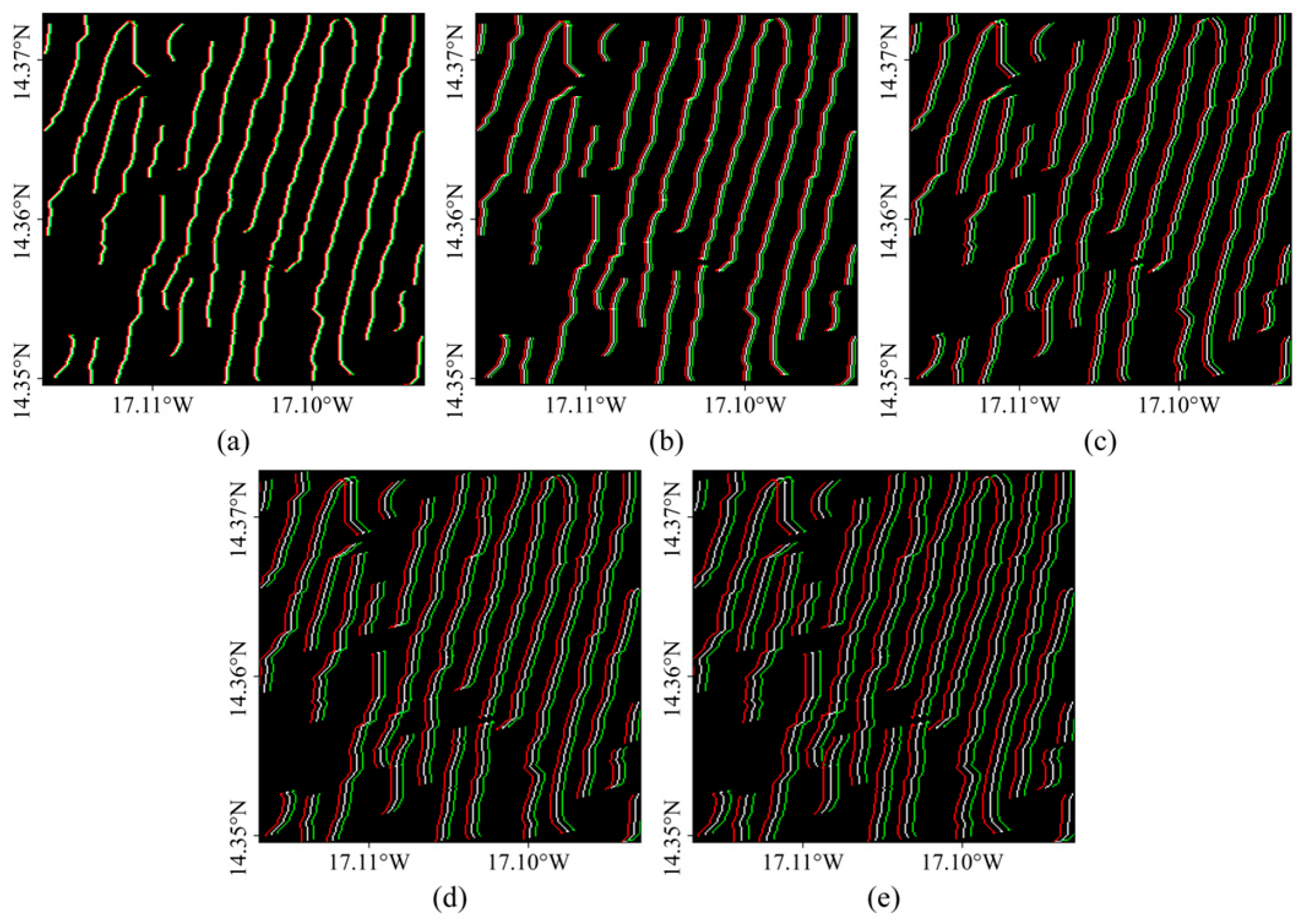
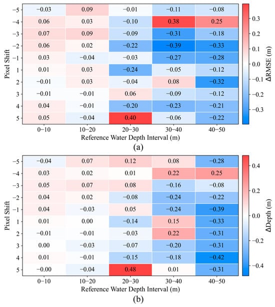
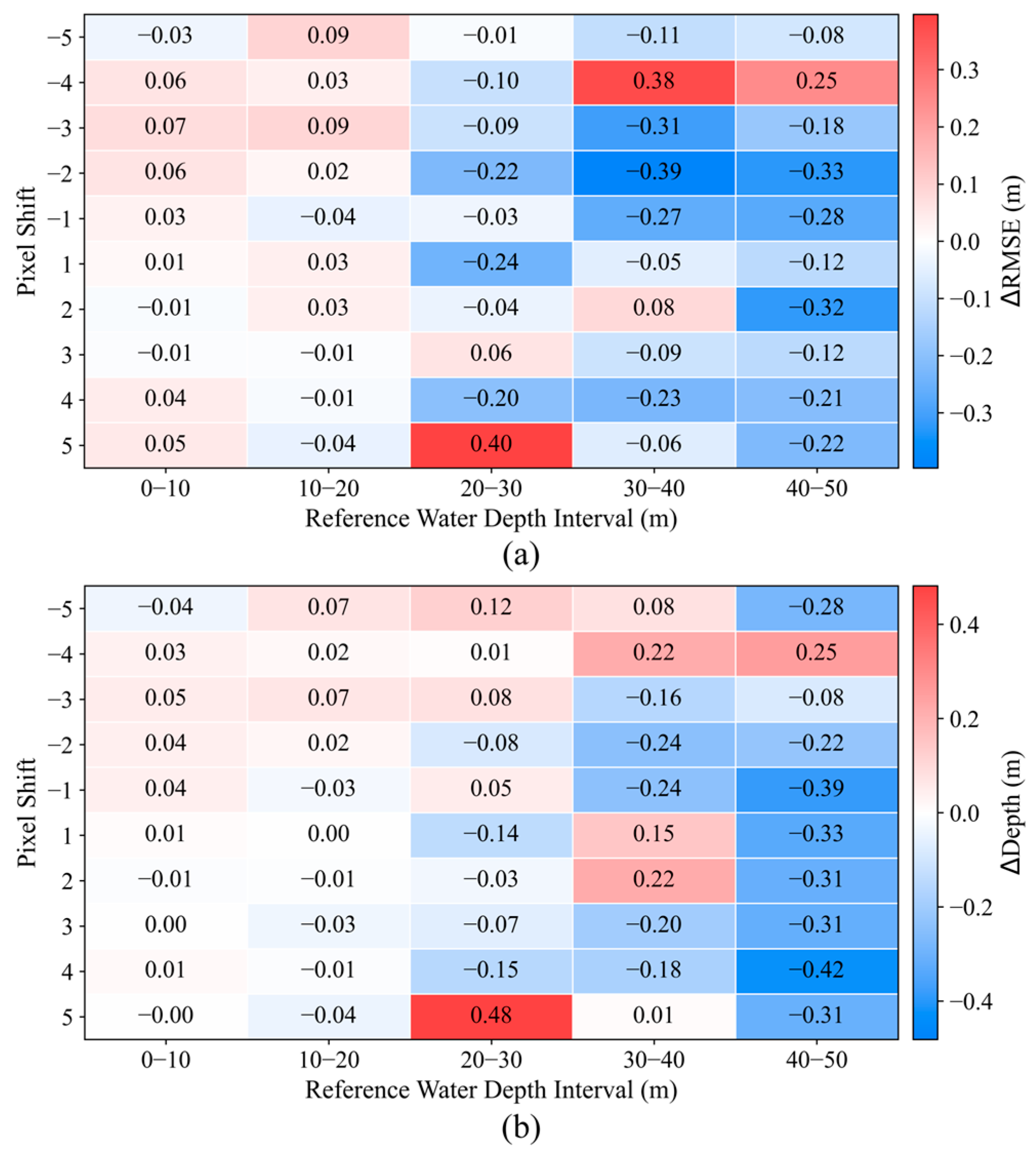
Positional errors in the wave-crest skeleton can directly affect local wavelength measurement and subsequent bathymetric retrieval. To evaluate the influence of pixel-level positioning errors, the original skeleton was shifted by ±1–5 pixels along the wave-propagation direction, with shoreward shifts defined as positive and offshore shifts as negative (Figure 17). These perturbations altered only the skeleton position while largely preserving its overall orientation and morphology, thereby simulating possible positioning errors introduced during stripe extraction. Across the different shift scenarios, both ΔRMSE and ΔDepth remain close to zero within the 0–20 m depth range, indicating limited sensitivity to small positioning errors in shallow water. Beyond 20 m, the response to skeleton displacement becomes more variable. The maximum absolute changes in RMSE and mean retrieved depth are 0.40 m and 0.48 m, respectively, both occurring for the +5-pixel shift in the 20–30 m interval. In the 40–50 m interval, most shifts produce negative changes in the mean retrieved depth, with the largest decrease reaching 0.42 m (Figure 18).
Figure 17.
Skeleton-offset map (20251109). (a–e) Superimposed wave-crest skeletons with offsets of ±1–5 pixels. Red indicates negative offsets, green indicates positive offsets, and white indicates the original skeleton.
Figure 18.
Error sensitivity analysis for different pixel offsets (20251109). (a) RMSE change in different depth segments; (b) mean retrieved-depth change in different depth segments.
The responses to positive and negative shifts are asymmetric, indicating that retrieval error does not vary linearly with skeleton displacement. This asymmetry may be related to local stripe morphology, adjacent-crest matching, and bathymetric gradients. Overall, the effects of crest-line positioning errors are small in the shallow-water intervals, whereas larger and more variable responses occur beyond approximately 20 m. Improving the reliability of skeleton positioning and crest matching therefore remains important for reducing retrieval errors in deeper water.
4.3. Influence of Tides and Currents
The retrieved water depth represents the instantaneous water depth at the Sentinel-1 acquisition time, whereas the GEBCO reference depth is referenced to mean sea level (MSL). Therefore, a tidal correction was applied to the retrieved depths to ensure consistency in the vertical datum. Tidal data were obtained from the SHOM Dakar tide-gauge station, for which water levels are available at a temporal resolution of 1 min. The tidal level corresponding to the Sentinel-1 acquisition time (19:18 UTC) was used for each scene. The SHOM tidal levels are referenced to the local hydrographic zero (ZH; zéro hydrographique). According to the vertical-datum information provided by SHOM for the Dakar station, mean sea level is 1.13 m above ZH. Therefore, the tidal level relative to mean sea level was calculated as ηMSL = ηZH − 1.13. The SAR-derived instantaneous water depth was then converted to the mean-sea-level reference using hMSL = hinst − ηMSL, where hinst is the instantaneous SAR-derived water depth and hMSL is the tide-corrected depth referenced to mean sea level. The ηMSL values corresponding to the acquisition times of the five Sentinel-1 images were 0.01, −0.53, −0.24, 0.43, and 0.24 m for image IDs 20230301, 20230313, 20251109, 20260201, and 20260213, respectively. Although tidal variations account for only a small fraction of the total depth in deeper water, they may introduce a relatively larger depth offset in shallow nearshore areas. Therefore, vertical-datum consistency and tidal-level correction are important for evaluating shallow-water retrieval accuracy.
In addition to tidal-level variations, background currents may influence bathymetric retrieval through wave–current interactions that modify wavelength and propagation direction. Background current velocity was not explicitly included in the present dispersion-relation-based retrieval, and its effect may therefore contribute to the remaining uncertainty, particularly in nearshore areas with relatively strong currents. Future work could incorporate in situ current measurements or hydrodynamic model outputs and apply a current-corrected dispersion relation to further assess retrieval errors under more complex hydrodynamic conditions.
4.4. Influence of Seabed Slope
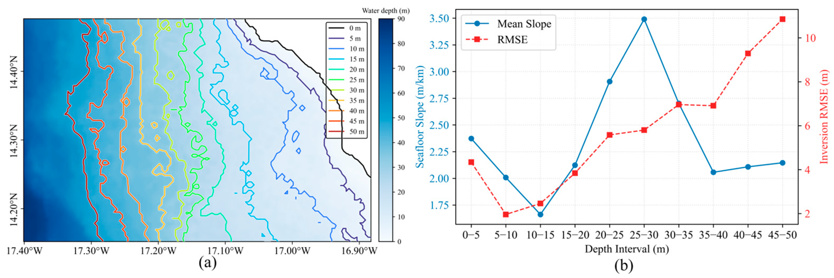
Seabed slope can affect wave refraction and local wavelength variability during wave propagation, thereby influencing dispersion-based bathymetric retrieval. To characterize seabed topographic variability in the study area, the two-dimensional seabed slope was calculated from the GEBCO reference depth as follows:
where h is the GEBCO reference depth, x and y are the east–west and north–south horizontal coordinates, respectively, and S (m/km) represents the magnitude of the horizontal depth gradient.
As shown in Figure 19a, the 0–50 m isobaths in the study area are generally parallel to the coastline, and water depth gradually increases from the nearshore zone to offshore waters. However, the spacing between isobaths varies among depth intervals. Figure 19b shows that the mean slope is lowest in the 10–15 m depth interval, then gradually increases and reaches a peak in the 25–30 m interval. Meanwhile, RMSE generally increases with depth, with a more pronounced increase beyond approximately 30 m. However, changes in seabed slope do not correspond directly to changes in RMSE. For example, the 25–30 m interval has the steepest mean slope but not the highest RMSE. Beyond 30 m, the mean slope decreases, whereas RMSE remains high. These results indicate that seabed slope affects retrieval error but is not the only controlling factor.
Figure 19.
Effect of seabed slope on bathymetric retrieval error. (a) GEBCO reference bathymetry; (b) mean seabed slope and RMSE across different depth intervals.
Steeper seabed slopes may enhance wave refraction and local wavelength variability, thereby increasing retrieval uncertainty. The larger errors observed in deeper water are also associated with the reduced depth sensitivity of the dispersion relation and the amplified effect of wavelength-estimation errors on depth inversion. Retrievals in areas of steep or rapidly varying topography should therefore be interpreted with greater caution and evaluated in the context of local seabed variability.
4.5. Applicability and Limitations
4.5.1. Applicability
The proposed method is primarily applicable to coastal waters where SAR imagery contains clear, continuous, and relatively periodic wave stripes, particularly in open-coast environments dominated by long-period swell and a relatively simple wave system. The results show that the method performs best within the 5–20 m depth range, while the absolute retrieval error increases with water depth. Therefore, the method is more suitable for shallow-water bathymetric retrieval under conditions of clearly visible wave stripes, whereas its application in complex wave fields or deeper waters should be treated with greater caution.
4.5.2. Main Limitations and Future Improvements
The proposed method is influenced by stripe quality, dominant wave period, and topographic conditions. Strong wind waves, breaking waves, crossing wave systems, reduced stripe contrast, and unstable stripe direction can interfere with skeleton extraction and crest matching, thereby reducing the reliability of wavelength estimation. A single dominant wave period cannot represent complex wave fields and may introduce systematic bias in deeper water. In addition, although tidal correction was applied, background current velocity, wave–current interaction, and nonlinear shallow-water wave effects were not considered. The spatial resolution and local accuracy of the GEBCO reference bathymetry also affect the accuracy assessment.
Future studies should use high-accuracy data, such as shipborne sounding, multibeam bathymetry, or high-resolution nautical charts, for independent validation. Wave reanalysis data and hydrodynamic models could also be incorporated to account for background-current effects and more complex wave systems. Cross-regional transfer experiments could be conducted in other open-coast environments to further evaluate the spatial transferability and generalizability of the proposed method. Further analysis of local stripe-extraction errors may also help explain the residual retrieval biases observed in some areas.
5. Conclusions
This study proposed a shallow-water bathymetry retrieval method based on Sentinel-1 SAR wave stripes. By integrating texture-preserving denoising, Gabor-filter enhancement, K-means stripe segmentation, Zhang–Suen skeleton extraction, and wavelength quality control, the method directly extracts local wave-crest lines from SAR images and retrieves water depth. The method was evaluated using five Sentinel-1 acquisitions to assess its multi-temporal applicability and robustness. The representative wave periods derived from the five SAR acquisitions ranged from 12.45 to 14.96 s.
Based on the mean performance across the five acquisitions, the cumulative 0–20 m depth range yielded an RMSE of 3.87 m, an MAE of 3.56 m, and a correlation coefficient of 0.95. When the cumulative depth range was extended to 0–50 m, the RMSE increased to approximately 6.06 m, while the correlation coefficient remained high at 0.97. Because no common valid samples were available at depths shallower than 5 m, the most stable retrieval performance was observed within the 5–20 m depth range, whereas retrieval errors generally increased with depth, particularly beyond 30 m. Error analysis indicated that uncertainty in the dominant wave period, crest-line positioning errors, stripe quality, background currents, and seabed-slope variability all influence retrieval accuracy, with stronger effects in deeper water. Overall, the method is suitable for open-coast environments with clear long-period swell and relatively simple wave systems and can support rapid shallow-water bathymetric mapping where in situ bathymetric data are limited.
Author Contributions
Conceptualization, Y.W. and S.L.; methodology, Y.W. and Y.Y.; software, Z.Y.; validation, Y.W. and Z.Y.; formal analysis, Y.W. and Y.Y.; investigation, Y.W. and Z.Y.; resources, S.L. and Y.Y.; data curation, Y.W. and Z.Y.; writing—original draft, Y.W. and Z.Y.; writing—review and editing, S.L. and Y.Y.; visualization, Z.Y. and Y.Y.; supervision, S.L.; project administration, S.L.; funding acquisition, S.L. All authors have read and agreed to the published version of the manuscript.
Funding
This research was funded by the National Natural Science Foundation of China (Grant No. 41976174) and the State Key Laboratory of Spatial Datum (Project No. SKLSD2025-KF-14).
Data Availability Statement
The Sentinel-1 SAR data used in this study are available from the Alaska Satellite Facility Data Search portal at https://search.asf.alaska.edu (accessed on 4 December 2025). The GEBCO reference bathymetry data are available from the GEBCO data service at https://betadownload.gebco.net (accessed on 17 June 2026). Tidal data were obtained from the French Naval Hydrographic and Oceanographic Service (SHOM) at https://data.shom.fr (accessed on 17 June 2026). Wave-period data were obtained from the Copernicus Marine Service (CMEMS) Global Ocean Waves Analysis and Forecast product, available at https://marine.copernicus.eu (accessed on 1 October 2026).
Acknowledgments
The authors would like to thank the Alaska Satellite Facility (ASF) for providing the Sentinel-1 SAR data, the GEBCO team for providing the reference bathymetry data, the French Naval Hydrographic and Oceanographic Service (SHOM) for providing the tidal data, and the Copernicus Marine Service (CMEMS) for providing the wave-period data used in this study. During the preparation of this manuscript, the authors used ChatGPT (GPT-5.6 Sol, OpenAI) to refine language expression and polish grammar. The AI tool was used under the authors’ supervision. All research ideas, experimental design, core data analysis, and scientific conclusions were independently completed by the authors. The authors have reviewed and edited the output and take full responsibility for the content of this publication.
Conflicts of Interest
The authors declare no conflicts of interest.
Abbreviations
The following abbreviations are used in this manuscript:
| GEBCO | General Bathymetric Chart of the Oceans |
| MAE | Mean absolute error |
| RMSE | Root mean square error |
| SHOM | Service hydrographique et océanographique de la Marine |
| VV | Vertical transmit–vertical receive polarization |
| PCA | Principal component analysis |
| SAR | Synthetic aperture radar |
References
- Salameh, E.; Frappart, F.; Almar, R.; Baptista, P.; Heygster, G.; Lubac, B.; Raucoules, D.; Almeida, L.P.; Bergsma, E.W.J.; Capo, S.; et al. Monitoring Beach Topography and Nearshore Bathymetry Using Spaceborne Remote Sensing: A Review. Remote Sens. 2019, 11, 2212. [Google Scholar] [CrossRef] [Scilit]
- Kutser, T.; Hedley, J.; Giardino, C.; Roelfsema, C.; Brando, V.E. Remote sensing of shallow waters—A 50 year retrospective and future directions. Remote Sens. Environ. 2020, 240, 111619. [Google Scholar] [CrossRef] [Scilit]
- Lyzenga, D.R. Passive remote sensing techniques for mapping water depth and bottom features. Appl. Opt. 1978, 17, 379–383. [Google Scholar] [CrossRef] [Scilit] [PubMed]
- Stumpf, R.P.; Holderied, K.; Sinclair, M. Determination of water depth with high-resolution satellite imagery over variable bottom types. Limnol. Oceanogr. 2003, 48, 547–556. [Google Scholar] [CrossRef] [Scilit]
- Caballero, I.; Stumpf, R.P. Towards Routine Mapping of Shallow Bathymetry in Environments with Variable Turbidity: Contribution of Sentinel-2A/B Satellites Mission. Remote Sens. 2020, 12, 451. [Google Scholar] [CrossRef] [Scilit]
- Mudiyanselage, S.D.; Wilkinson, B.; Abd-Elrahman, A. Automated High-Resolution Bathymetry from Sentinel-1 SAR Images in Deeper Nearshore Coastal Waters in Eastern Florida. Remote Sens. 2024, 16, 1. [Google Scholar] [CrossRef] [Scilit]
- Alpers, W.; Hennings, I. A theory of the imaging mechanism of underwater bottom topography by real and synthetic aperture radar. J. Geophys. Res. Oceans 1984, 89, 10529–10546. [Google Scholar] [CrossRef] [Scilit]
- Calkoen, C.J.; Hesselmans, G.H.F.M.; Wensink, G.J.; Vogelzang, J. The Bathymetry Assessment System: Efficient depth mapping in shallow seas using radar images. Int. J. Remote Sens. 2001, 22, 2973–2998. [Google Scholar] [CrossRef]
- Alpers, W.R.; Ross, D.B.; Rufenach, C.L. On the detectability of ocean surface waves by real and synthetic aperture radar. J. Geophys. Res. Oceans 1981, 86, 6481–6498. [Google Scholar] [CrossRef] [Scilit]
- Hasselmann, K.; Raney, R.K.; Plant, W.J.; Alpers, W.; Shuchman, R.A.; Lyzenga, D.R.; Rufenach, C.L.; Tucker, M.J. Theory of synthetic aperture radar ocean imaging: A MARSEN view. J. Geophys. Res. Oceans 1985, 90, 4659–4686. [Google Scholar] [CrossRef] [Scilit]
- Holland, K.T. Application of the linear dispersion relation with respect to depth inversion and remotely sensed imagery. IEEE Trans. Geosci. Remote Sens. 2001, 39, 2060–2072. [Google Scholar] [CrossRef] [Scilit]
- Fan, K.; Huang, W.; He, M.; Fu, B.; Zhang, B.; Chen, X. Depth inversion in coastal water based on SAR image of waves. Chin. J. Oceanol. Limnol. 2008, 26, 434–439. [Google Scholar] [CrossRef] [Scilit]
- Brusch, S.; Held, P.; Lehner, S.; Rosenthal, W.; Pleskachevsky, A. Underwater bottom topography in coastal areas from TerraSAR-X data. Int. J. Remote Sens. 2011, 32, 4527–4543. [Google Scholar] [CrossRef] [Scilit]
- Bian, X.; Shao, Y.; Wang, S.; Tian, W.; Wang, X.; Zhang, C. Shallow Water Depth Retrieval from Multitemporal Sentinel-1 SAR Data. IEEE J. Sel. Top. Appl. Earth Obs. Remote Sens. 2018, 11, 2991–3000. [Google Scholar] [CrossRef] [Scilit]
- Bian, X.; Shao, Y.; Zhang, C.; Xie, C.; Tian, W. The feasibility of assessing swell-based bathymetry using SAR imagery from orbiting satellites. ISPRS J. Photogramm. Remote Sens. 2020, 168, 124–130. [Google Scholar] [CrossRef] [Scilit]
- Cloarec, M.; Roeber, V.; Ranchin, T.; Dubranna, J. Extraction of bathymetric features using multiple SAR images produced by Sentinel-1. In Proceedings of the Sixth International Conference on Remote Sensing and Geoinformation of the Environment (RSCy2018), Paphos, Cyprus, 26–29 March 2018; SPIE: Bellingham, WA, USA, 2018; Volume 10773, pp. 274–282. [Google Scholar] [CrossRef] [Scilit]
- Pleskachevsky, A.; Lehner, S.; Heege, T.; Mott, C. Synergy and fusion of optical and synthetic aperture radar satellite data for underwater topography estimation in coastal areas. Ocean Dyn. 2011, 61, 2099–2120. [Google Scholar] [CrossRef] [Scilit]
- Boccia, V.; Renga, A.; Rufino, G.; D’Errico, M.; Moccia, A.; Aragno, C.; Zoffoli, S. Linear Dispersion Relation and Depth Sensitivity to Swell Parameters: Application to Synthetic Aperture Radar Imaging and Bathymetry. Sci. World J. 2015, 2015, 374579. [Google Scholar] [CrossRef] [Scilit] [PubMed]
- Boccia, V.; Renga, A.; Moccia, A.; Zoffoli, S. Tracking of Coastal Swell Fields in SAR Images for Sea Depth Retrieval: Application to ALOS L-Band Data. IEEE J. Sel. Top. Appl. Earth Obs. Remote Sens. 2015, 8, 3532–3540. [Google Scholar] [CrossRef] [Scilit]
- Huang, L.; Meng, J.; Fan, C.; Zhang, J.; Yang, J. Shallow Sea Topography Detection from Multi-Source SAR Satellites: A Case Study of Dazhou Island in China. Remote Sens. 2022, 14, 5184. [Google Scholar] [CrossRef] [Scilit]
- Huang, L.; Fan, C.; Meng, J.; Yang, J.; Zhang, J. Shallow sea topography detection using fully polarimetric Gaofen-3 SAR data based on swell patterns. Acta Oceanol. Sin. 2023, 42, 150–162. [Google Scholar] [CrossRef] [Scilit]
- Wiehle, S.; Pleskachevsky, A.; Gebhardt, C. Automatic bathymetry retrieval from SAR images. CEAS Space J. 2019, 11, 105–114. [Google Scholar] [CrossRef] [Scilit]
- Pereira, P.; Baptista, P.; Cunha, T.; Silva, P.A.; Romão, S.; Lafon, V. Estimation of the nearshore bathymetry from high temporal resolution Sentinel-1A C-band SAR data—A case study. Remote Sens. Environ. 2019, 223, 166–178. [Google Scholar] [CrossRef] [Scilit]
- Santos, D.; Fernández-Fernández, S.; Abreu, T.; Silva, P.A.; Baptista, P. Retrieval of nearshore bathymetry from Sentinel-1 SAR data in high energetic wave coasts: The Portuguese case study. Remote Sens. Appl. Soc. Environ. 2022, 25, 100674. [Google Scholar] [CrossRef] [Scilit]
- Hao, M.; Shao, W.; Hu, Y.; Migliaccio, M.; Jiang, X. Nearshore topography retrieval based on wave spectrum inverted from Gaofen-3 image. Geo-Spat. Inf. Sci. 2026, 29, 1046–1058. [Google Scholar] [CrossRef] [Scilit]
- Zhang, M.; Qi, C.; Yang, F.; Wang, R.; Pirasteh, S. Enhancing water depth inversion accuracy via SAR and variable window sliding segmentation. Front. Mar. Sci. 2025, 12, 1509503. [Google Scholar] [CrossRef] [Scilit]
- Diao, L.; Xu, Y.; Zhao, Y.; Mo, H.; Du, Y.; Qiu, X.; Chong, J. Nearshore bathymetry estimation from SAR imagery based on the adaptive window guided by local wave direction. Int. J. Remote Sens. 2026, 47, 3967–3999. [Google Scholar] [CrossRef] [Scilit]
- Santos, D.; Abreu, T.; Silva, P.A.; Baptista, P. Estimation of Coastal Bathymetry Using Wavelets. J. Mar. Sci. Eng. 2020, 8, 772. [Google Scholar] [CrossRef] [Scilit]
- Zhao, W.; Zhou, G.; Yue, T.; Yang, B.; Tao, X.; Huang, J.; Yang, C. Retrieval of ocean wavelength and wave direction from SAR image based on Radon transform. In Proceedings of the 2013 IEEE International Geoscience and Remote Sensing Symposium (IGARSS), Melbourne, Australia, 21–26 July 2013; IEEE: Piscataway, NJ, USA, 2013; pp. 1513–1516. [Google Scholar] [CrossRef] [Scilit]
- Lee, J.S.; Jurkevich, L.; Dewaele, P.; Wambacq, P.; Oosterlinck, A. Speckle filtering of synthetic aperture radar images: A review. Remote Sens. Rev. 1994, 8, 313–340. [Google Scholar] [CrossRef] [Scilit]
- Park, J.-W.; Won, J.-S.; Korosov, A.A.; Babiker, M.; Miranda, N. Textural Noise Correction for Sentinel-1 TOPSAR Cross-Polarization Channel Images. IEEE Trans. Geosci. Remote Sens. 2019, 57, 4040–4049. [Google Scholar] [CrossRef] [Scilit]
- Cui, A.; Ma, Y.; Zhang, J.; Wang, R. A SAR wave-enhanced method combining denoising and texture enhancement for bathymetric inversion. Int. J. Appl. Earth Obs. Geoinf. 2025, 139, 104520. [Google Scholar] [CrossRef] [Scilit]
- Sahoo, A.; Nechifor, V.; Ferrari, E.; Ferreira, V.; Amany, D.S.D. On the positive economic impacts of port infrastructure development and seaborne trade efficiencies in Sub-Saharan Africa: The case of Senegal. Marit. Econ. Logist. 2025, 27, 525–548. [Google Scholar] [CrossRef] [Scilit]
- Deme, E.H.B.; Deme, M.; Failler, P. Small pelagic fish in Senegal: A multi-usage resource. Mar. Policy 2022, 141, 105083. [Google Scholar] [CrossRef] [Scilit]
- Cissé, C.O.T.; Marić, I.; Domazetović, F.; Glavačević, K.; Almar, R. Derivation of Coastal Erosion Susceptibility and Socio-Economic Vulnerability Models for Sustainable Coastal Management in Senegal. Sustainability 2024, 16, 7422. [Google Scholar] [CrossRef] [Scilit]
- Samou, M.S.; Bertin, X.; Sakho, I.; Lazar, A.; Sadio, M.; Diouf, M.B. Wave Climate Variability along the Coastlines of Senegal over the Last Four Decades. Atmosphere 2023, 14, 1142. [Google Scholar] [CrossRef] [Scilit]
- Papafitsoros, K.; Schönlieb, C.-B. A combined first and second order variational approach for image reconstruction. J. Math. Imaging Vis. 2014, 48, 308–338. [Google Scholar] [CrossRef] [Scilit]
- Jung, H.; Kim, Y.; Jang, H.; Ha, N.; Sohn, K. Unsupervised deep image fusion with structure tensor representations. IEEE Trans. Image Process. 2020, 29, 3845–3858. [Google Scholar] [CrossRef] [Scilit] [PubMed]
- Manjunath, B.S.; Ma, W.Y. Texture features for browsing and retrieval of image data. IEEE Trans. Pattern Anal. Mach. Intell. 1996, 18, 837–842. [Google Scholar] [CrossRef] [Scilit]
- Daugman, J.G. Uncertainty relation for resolution in space, spatial frequency, and orientation optimized by two-dimensional visual cortical filters. J. Opt. Soc. Am. A 1985, 2, 1160–1169. [Google Scholar] [CrossRef] [Scilit] [PubMed]
- Qi, K.-T.; Zhang, H.-S.; Zheng, Y.-G.; Zhang, Y.; Ding, L.-Y. Stripe segmentation of oceanic internal waves in SAR images based on Gabor transform and K-means clustering. Oceanologia 2023, 65, 548–555. [Google Scholar] [CrossRef] [Scilit]
- MacQueen, J.B. Some methods for classification and analysis of multivariate observations. In Proceedings of the Fifth Berkeley Symposium on Mathematical Statistics and Probability; Le Cam, L.M., Neyman, J., Eds.; University of California Press: Berkeley, CA, USA, 1967; Volume 1, pp. 281–297. [Google Scholar]
- Haralick, R.M.; Sternberg, S.R.; Zhuang, X. Image Analysis Using Mathematical Morphology. IEEE Trans. Pattern Anal. Mach. Intell. 1987, PAMI-9, 532–550. [Google Scholar] [CrossRef] [Scilit] [PubMed]
- Zhang, T.Y.; Suen, C.Y. A fast parallel algorithm for thinning digital patterns. Commun. ACM 1984, 27, 236–239. [Google Scholar] [CrossRef] [Scilit]
- Saeed, K.; Tabędzki, M.; Rybnik, M.; Adamski, M. K3M: A universal algorithm for image skeletonization and a review of thinning techniques. Int. J. Appl. Math. Comput. Sci. 2010, 20, 317–335. [Google Scholar] [CrossRef] [Scilit]
- Solís Montero, A.; Lang, J. Skeleton pruning by contour approximation and the integer medial axis transform. Comput. Graph. 2012, 36, 477–487. [Google Scholar] [CrossRef] [Scilit]
- Xu, Z.; Zhu, S.; Zhang, W.; Kang, Y.; Wu, X. Outlier Correction in Remote Sensing Retrieval of Ocean Wave Wavelength and Application to Bathymetry. Remote Sens. 2025, 17, 3284. [Google Scholar] [CrossRef] [Scilit]

Disclaimer/Publisher’s Note: The statements, opinions and data contained in all publications are solely those of the individual author(s) and contributor(s) and not of MDPI and/or the editor(s). MDPI and/or the editor(s) disclaim responsibility for any injury to people or property resulting from any ideas, methods, instructions or products referred to in the content. |
© 2026 by the authors. Licensee MDPI, Basel, Switzerland. This article is an open access article distributed under the terms and conditions of the Creative Commons Attribution (CC BY) license.