


Abstract
Remote sensing is essential for mapping mangrove forest ecosystems, yet accuracy and spatial resolution remain limited, particularly in Africa, where mangroves are fragmented, reference data and cloud-free images are scarce. The state-of-the-art of mangrove forest mapping relies on native-resolution imagery using machine learning. This study evaluates deep learning methods using aggregated multi-date satellite imagery to improve mangrove mapping and national-scale area estimation. Super-resolution and semantic segmentation techniques were applied to Sentinel-2 (S2) and Sentinel-1 (S1) images, with training data derived from field observations and high-resolution drone and satellite imagery. Coastal regions of Tanzania and Ghana were used as representative study areas for eastern and western Africa, respectively. Results show strong classification performance, with S2 imagery alone achieving an Intersection over Union (IoU) of 85.8%. Adding S1 provided modest gains (IoU 86.3%), while super-resolution significantly improved the accuracy (IoU 88.5%). The combined super-resolved S2 and S1 dataset yielded the highest performance (IoU 89.2%). Wall-to-wall mapping and statistically rigorous validation and area estimation produced accurate results with quantified uncertainty. Tanzania showed high consistency (F1 = 96%; 1207 km2, 95% CI [1151.7, 1263]), while Ghana exhibited slightly higher uncertainty (F1 = 92%; 92.6 km2, 95% CI [87.5, 97.7]). Integrating deep learning with multi-date, multi-sensor fusion and super-resolution enables accurate mangrove mapping and area estimation for improved coastal management and restoration.
Keywords:
deep learning; U-Net; Xception; Resnet; Tanzania mangroves; Ghana mangroves; forest area estimation 1. Introduction
Mangroves are woody trees and shrubs that inhabit intertidal zones of tropical and temperate regions, typically occurring at the interface between land and sea [1]. They occupy sheltered coastlines such as estuaries, river deltas, and shallow lagoons [2]. Mangrove ecosystems provide a wide range of critical ecological services [3]. They stabilize coastlines, reduce erosion, buffer storm surges, and mitigate flooding [4,5]. They serve as nursery habitats for fish, crustacean, and bird species, thereby supporting marine biodiversity and sustaining local fisheries [6,7]. Mangroves also play a significant role in climate regulation through long-term carbon sequestration and in maintaining water quality, which supports both ecological health and coastal livelihoods [8,9].
Despite their immense value, mangrove forests are increasingly threatened by anthropogenic activities and climate-related pressures. The State of the World’s Mangroves 2024 report [10] highlights accelerating losses due to coastal development activities such as aquaculture, rice cultivation, oil palm expansion, urban settlements, and wood extraction. Pollution from agricultural runoff, industrial discharges, and plastics further degrades mangrove habitats [9]. Climate change compounds these threats through sea-level rise, increased storm intensity, and altered salinity regimes, all of which impair mangrove health and survival [11,12]. Without effective conservation and sustainable management interventions, continued degradation could result in substantial loss of mangrove extent, and the critical ecosystem functions they provide.
Given these values and risks, accurate and detailed mapping of mangrove forests is essential for monitoring change, guiding conservation planning, and supporting sustainable ecosystem management. Remote sensing is widely recognized as an indispensable tool for mapping and monitoring forest resources in general, and mangrove ecosystems in particular. Ying and Wang [13] provide a comprehensive synthesis of remote-sensing approaches for large-scale mangrove studies, noting that despite technological improvements, challenges remain due to limited field samples and the coarse resolution of some globally available imagery. The Global Mangrove Watch (GMW) initiative addressed part of this gap by producing a global baseline map of mangrove extent starting in 2010 [14,15,16,17] using a combination of ALOS PALSAR radar data, Landsat imagery, and machine-learning classification. While highly valuable, GMW’s accuracy varies regionally, with African mangrove areas being particularly affected by lack of adequate reference data. African mangrove forests are also known to be highly fragmented with great regional variations. Alternative continental and national map datasets are scanty in Africa.
To improve mangrove forest mapping in West Africa, Liu et al. [18] combined Sentinel-2 (S2) and Sentinel-1 (S1) imagery with three machine-learning models, producing 20 m resolution mangrove maps with high accuracy. Similarly, Lombard et al. [19] mapped mangrove zonation across West Africa using S2 imagery and a Random Forest (RF) classifier, achieving high accuracy at 10 m resolution. Other studies, in other regions, have made efforts to advance methodological innovations. Chen et al. [20] developed the Red-Edge Mangrove Index (REMI) that outperformed six common indices in detecting mangroves on Hainan Island using S2 spectral bands. Chan-Bagot et al. [21] demonstrated that combining optical (Landsat-8, S2) and S1 data with a RF model yields the highest annual mapping accuracy in Guyana, enabling the identification of previously undetected mangrove loss. Mandal et al. [22] examined reproducibility challenges in automated mapping, finding notable variation across models and algorithm runs. They introduced the “Places of Agreement” framework to highlight areas mapped consistently, emphasizing the need for caution in decision-making.
At even finer scales, Zhang et al. [23] produced a 0.2 m resolution mangrove map for Hong Kong by applying the deep learning framework DeepLabV3+, on aerial imagery, then simulated coarser resolutions to analyze scale effects. They found sharp drops in accuracy at 10 m and 30 m resolutions, identifying 6 m resolution as optimal. Wei et al. [24] used very high-resolution satellite images for mapping mangrove forest extent, and their results support the conclusions of Zhang et al. [22]. Chen et al. [25] used a novel super-resolution model combined with the RF classifier to map mangroves at 10 m spatial resolution from Landsat 5 images and reported an improved accuracy when using super-resolution. Hong et al. [26] tested different super-resolution models to enhance Landsat 8 images to 10 m for mapping mangrove forests, showing that super-resolved imagery can substantially improve classification accuracy. However, application of super-resolution to S1 and S2 images and use of deep learning in classification and segmentation of mangroves from satellite images remain unexplored.
These studies collectively demonstrate substantial progress in mangrove mapping. However, they also reveal persistent challenges related to geographic transferability, spatial resolution, dependence on limited field reference data, and the limited adoption of advanced deep learning approaches. Remaining research gaps include the following challenges: (1) Many regional studies rely on single-date and mono-sensor imagery rather than multi-temporal and multi-sensor approaches. Cloud cover in tropical regions is known to restrict the practicality of single-date imagery and the possibility of time-series analysis. (2) Coarse spatial resolution images fail to detect fragmented mangrove forest stands that are widespread in Africa; and methods of improving spatial resolution have not gone beyond 10 m which is already generically provided by S2 satellites. (3) Insufficient field data for reference and validation remains a major constraint globally and is especially acute in Africa. (4) The advantages offered by more complex deep learning architectures, particularly convolution-based models, are not utilized in mangrove mapping, attributed to limited reference data, as most of the applications hitherto widely implement spectral indices and machine-learning methods such as RF.
Addressing these data and methodological gaps identified above will enable more detailed and accurate mapping of mangrove forests, with direct benefits for mangrove ecosystem restoration and conservation in Ghana and Tanzania. For instance, reducing misclassification errors improves the accuracy of mangrove extent maps, supporting more reliable estimates of biomass and carbon stocks, and better-targeted restoration investments. More reliable maps, further, allow managers to prioritize restoration sites, allocate limited resources more efficiently, and strengthen monitoring of mangrove ecosystem change.
This study seeks to advance the accuracy and spatial detail of mangrove forest mapping by integrating optical and radar satellite data, leveraging multi-temporal image stacks, applying advanced deep learning techniques for enhancing spatial resolution and classification. It demonstrates the use of convolutional neural network (CNN)-based semantic segmentation on median-aggregated multi-date satellite imagery. Using native-resolution S2 data as a baseline, the study investigates how the added value of:
- applying segmentation-based deep learning models,
- enhancing spatial resolution through super-resolution techniques, and
- integrating radar (S1) and optical (S2) datasets can improve fine-scale mangrove mapping and produce statistically reliable national-scale area estimations for better mangrove management including conservation and restoration.
2. Study Areas
Mangrove forests in Africa occur predominantly along the western and eastern coasts of the continent, where suitable climatic and hydrological conditions support their growth. To capture the ecological variability between these two major mangrove regions, this study focuses on two sites: the coastal region of Tanzania in Eastern Africa and the coastal region of Ghana in Western Africa. Figure 1 illustrates the national boundaries of Ghana and Tanzania highlighting the location of the study areas.
Figure 1.
Location of the study areas in the African continent, Ghana in west and Tanzania in east, and their respective coastal zones zoomed in.
Although the two countries were not selected through a statistically stratified sampling framework, they were chosen because they represent distinct biogeographical regions of African mangroves and encompass differing environmental conditions, including rainfall patterns, tidal regimes, riverine influences, and degrees of anthropogenic pressure [27,28,29]. Mangrove ecosystems in Ghana are generally sparse, highly fragmented, and degraded in many areas, with increasing encroachment by competitive fern species and other shrubs. In contrast, Tanzanian mangroves are comparatively lush, well preserved and structurally robust, particularly within protected areas such as the Rufiji delta, where dense and extensive stands remain intact. However, climate-related disturbances and anthropogenic activities, including mining, agricultural expansion, and other forms of land-use change, are increasingly encroaching on mangrove habitats in many areas. These ecological and environmental contrasts provide a valuable opportunity to evaluate and demonstrate the challenges and applicability of mangrove mapping and monitoring approaches across diverse landscape and management contexts.
For both countries, the coastal zone was delineated using a 10 km inland buffer from their respective coastlines. This approach ensures comprehensive coverage of all mangrove ecosystems while minimizing the inclusion of inland areas that do not support mangrove vegetation. In areas where river estuaries allow inland encroachment of mangroves, the buffer zone is extended inland along the river system.
3. Materials and Methods
3.1. Datasets
3.1.1. Ancillary Data
A comprehensive review of existing secondary data sources on mangrove forests was undertaken to gain initial understanding of the spatial distribution and general locations of mangrove ecosystems along the African coast. To support this assessment, two global datasets were employed: the GMW Version 4 which is based on satellite images from the year 2020 [14] and the ESA world cover 2021 product [30]. Together, these datasets supported the broader methodological workflow by offering generalized mangrove extent maps that guided fieldwork planning and facilitated the initial manual delineation of mangrove forests in Tanzania and Ghana.
3.1.2. Satellite Images
Stacked multi-date S1 and S2 satellite imagery from the European Union’s Copernicus Program were used as primary image datasets. Image datasets covering the coastal regions of Tanzania and Ghana during their respective dry seasons were obtained from the Digital Earth Africa (DEA) Analysis-Ready Data cube (ARD). DEA is a web-based platform that provides ARD and decision-ready products that transform satellite data into actionable insights for sustainable development across Africa [31].
Multi-date image stacks from the DEA ARD products were chosen as the study areas experience frequent cloud cover, making it extremely challenging to acquire cloud-free single-date scenes. Dry season images were chosen to enhance the contrast between areas covered by mangrove forests and other vegetation types. The choice of dry season has additional advantage of reducing the effects of tides and seasonal flooding and providing greater proportion of cloud-free image coverage. For Tanzania, all S1 and S2 images acquired from July to October 2024 were used, while for Ghana images acquired from November 2024 to March 2025 were selected.
The S2 images in DEA are stored from the Copernicus Level-2A products, and clouds and shadows are masked automatically using the Scene Classification Layer (SCL). The S2 bands are rescaled using the Min–Max normalization method to values between 0 and 1, considering a generally chosen maximum value of 10,000 and minimum value of 0. The S1 is acquired from a C-band Synthetic Aperture Radar (SAR) satellite operating in an interferometric Wide Swath acquisition mode with dual polarization. In DEA S1 dataset is radiometrically corrected from both ascending and descending orbits and provided as dimensionless linear gamma-naught (γ°) backscatter, not as decibels. However, no speckle filtering is applied. The two bands of S1, VV and VH, are left as they are in floating numbers with most values falling between 0 and 1, and a few extremes going beyond 1. Values above 1 in some outlying pixels are cut to 1.
Temporal median composites were generated for each pixel across all VNIR, Red-Edge, and SWIR bands of S2, as well as the VV and VH backscatter channels of S1, at 10 m spatial resolution. DEA ARD stores both products at 10 m by interpolating the lower resolution bands. The number of dry season time stamps for both countries ranges from 27 to 32. However, the number of pixel-wise valid timestamps vary depending on cloud coverage. Temporal median compositing was then performed using the DEA Sandbox which helps reduce the effects of residual cloud, haze, shadow artifacts, and occasional tides and floods, providing a stable spectral representation of each pixel during the dry season.
3.1.3. Field Data
Field campaigns were planned for both Ghana and Tanzania. However, an actual field visit was conducted only in Ghana, as logistic obstacles delayed field visit in Tanzania indefinitely. After reviewing the ancillary data, areas of interest (AoIs) were selected for field observation. Although the general strategy used for reference data collection was random sampling, AoIs for the field campaign were selected based on mangrove forest abundance, physical accessibility, mangrove forest fragmentation, boundaries of mangrove and non-mangrove forests, and difficulty of identifying mangroves from other sources. Two estuarine systems in Ghana were selected for the field campaign based on the abundance of mangrove forests: namely, the Ankobra River estuarine system in the west and the Volta River estuarine system in the east. During the field visits, mangrove forest boundaries were visually identified and manually delineated with the aid of high-resolution Google Satellite and Google Earth Pro imagery on the background to define the extent. The QField software (version 4.3.5) integrated with QGIS (version 4.2.2) was used for the visualization and delineation of the training data. Boats were used to access mangroves from the marine and river sides, while vehicles and walking surveys were used on the landward side.
Sites that could not be reached during field campaigns were observed using drone imagery. Drone flights were carried out in thus selected locations, capturing high-resolution image strips. The DJI Mavic 3 drone with RTK on board was used for the flight. The details of the drone flights instrumentation and image acquisition are summarized in Table 1. The drone images were later orthorectified using the Pix4D software (version 4.10.1) to support precise delineation of mangrove boundaries. The orthorectified drone images were then used to manually delineate mangrove polygons, particularly in areas where field observation was not feasible and satellite imagery alone did not provide sufficient detail.
Table 1.
Description of the specifications of the drone imagery and instrumentation.
Based on the experiences and insights gained from field observations and drone imagery, additional training data were delineated manually using multiple data sources to further expand and refine the mangrove training dataset. To guide this process and ensure representation of diverse mangrove environments, the GMW maps were used to identify mangrove-rich regions and focus delineation efforts accordingly. While local boundary precision varied across sources, the primary objective was to build a large, diverse, and robust training dataset suitable for deep learning, where minor boundary inconsistencies are typically handled by complex model architectures. Therefore, no formal statistical sampling design was imposed in all reference data collection; instead, reference samples were collected randomly from locations where mangroves and non-mangroves could be reliably interpreted. Combinations of Google Earth Pro, Google Satellite, and S2 false-color composites were used to identify the boundaries of mangrove forests.
For Tanzania, training data were derived exclusively from manual interpretation of Google Earth Pro imagery and S2 composites. Only a few post-classification validation points were checked in the field. Dense and high-canopy mangrove forests are readily identifiable in high-resolution Google Earth Pro imagery as well as in S2 red-edge and SWIR false-color composites. All the manual delineations were ultimately merged with those derived from drone images and field observation to create series of polygons in both Tanzania and Ghana.
3.2. Super-Resolution of Satellite Images
To enhance the images to a higher spatial resolution, a single image super-resolution (SISR) method was used. SISR aims to reconstruct a high-resolution image from a single low-resolution input, making it a valuable technique when corresponding high-resolution reference images are unavailable. It uses down-sampled version of the images as the input low-resolution dataset and learns to reconstruct the original native-resolution image. Although SISR is inherently an ill-posed problem with recognized limitations in preserving fine spatial details [32], it has demonstrated considerable utility in remote-sensing applications in the absence of target high-resolution images. In this study, SISR was implemented using a Generative Adversarial Network (GAN) modified from the Enhanced Super-Resolution GAN (ESRGAN) model [33]. The ESRGAN architecture employs a generator to produce higher-resolution images and a discriminator to distinguish between generated and real images, enabling the reconstruction of sharper textures and finer structural details than conventional interpolation methods. The details of the modifications applied to the model and the implementation procedure of SISR are described in [34]. Here, the model was reconstructed to fit to 11-bands images to enhance the resolution by five times to spatial resolution of 2 m. The upscaling layer in the network is thus modified to enhance the image resolution by five times. Additional modifications are made to the training pipeline as explained below.
The model was trained on the median-aggregated multi-date images described above covering coastal regions of East and West Africa, extending beyond the specific study areas to improve generalization. Although the extraction of the median-aggregated dataset was conducted in the DEA platform, training of the modified ESRGAN model was conducted at our local High-Performance Computing (HPC) facility with Graphic Processing Units (GPUs).
The ESRGAN model was pipelined to train using a combination of pixel reconstruction loss, perceptual loss, and relativistic adversarial loss. Pixel loss was computed as the mean squared error (MSE) between generated and ground-truth high-resolution images. Perceptual loss was calculated from the MSE between VGG feature representations of generated and target images, enabling the network to preserve perceptually important image structures and textures. A Relativistic Average Generative Adversarial Network (RaGAN) objective was employed to improve image realism. The total generator loss was defined as the weighted sum of pixel-wise, perceptual and adversarial losses [35],. Model performance was evaluated using Peak Signal-to-Noise Ratio (PSNR), while discriminator loss, generator loss, perceptual loss, and pixel loss were monitored throughout training. Both generator and discriminator were optimized using the Adam optimizer with an exponentially decaying learning-rate schedule initialized at , with a decay rate of 0.9 every 1000 training steps. The model was trained with 100 steps per epoch. Once trained, the model was later used during training of the segmentation model and prediction.
The performance of the ESRGAN model was quantitatively evaluated on a set of test data using widely adopted image reconstruction metrics, including Peak Signal-to-Noise Ratio (PSNR), Structural Similarity Index Measure (SSIM), Learned Perceptual Image Patch Similarity (LPIPS) and Spectral Angle Mapping (SAM). Because LPIPS is designed for three-channel imagery to evaluate visual similarity, it was computed only for the three visible bands of the S2 in this study as well. These metrics assess both the fidelity and perceptual quality of the super-resolved images. Model performance was evaluated on a set of test tiles independent of the training, and summary statistics were derived to assess the overall reconstruction accuracy and generalization capability of the model.
Two image datasets, based on their spatial resolution, were then created, namely the original S2 images and their super-resolved version. Two other datasets were also defined based on whether S1 bands are included or not, together making four datasets.
3.3. Implementation of Binary Semantic Segmentation
3.3.1. Preparation of Training Data
Semantic segmentation requires extensive training datasets consisting of paired tiles of images and corresponding masks (e.g., Figure 2). The training datasets were first converted to binary raster masks, where mangrove areas were encoded as foreground and all other land-cover types as background. After mask creation, both the multispectral imagery and their masks were divided into non-overlapping fixed-size tiles of 160 × 160 pixels. Each mask tile was paired with its corresponding multispectral image tile, ensuring spatial alignment between inputs and labels. In total, 1625 image–mask tile pairs were generated for the 10 m datasets.
Figure 2.
An example of satellite image (left) and mask (right) tile pairs: Mangroves in yellow and non-mangroves in dark purple.
Each of the training tiles contained both mangrove and non-mangrove pixels, although the proportions vary considerably from tile to tile. As the training data from which the tiles were constructed were collected randomly and depending on interpretability and accessibility, spatial independence was not strictly enforced. However, the tiles were non-overlapping, although proximity and adjacency were not avoidable.
3.3.2. The Semantic Segmentation Model
A U-Net model for binary segmentation was constructed using the Xception model [36] as the encoder and part of the ResNet model [37] as decoder, as described in [34]. This hybrid architecture forms a deep U-Net model with many parameters, enabling it to capture both fine-scale spatial features and broader contextual patterns. The U-Net model has 263 layers and over 38 million trainable parameters. The Xception encoder provides efficient feature extraction through depth-wise separable convolutions, reducing computational cost while maintaining strong representational capacity. The ResNet-based decoder enhances gradient flow during training through residual connections, improving stability and supporting accurate reconstruction of spatial details in the segmentation output. By combining the strengths of both architectures, the architecture has shown to achieve high segmentation accuracy on satellite images [34]. The model is also closely related to the DeepLabV3+ model [38], known for high accuracy in image segmentation, in that it involves both ResNet and Xception as backbones and utilizes the depth-wise separable convolution.
The U-Net model was compiled using a composite loss function that combines Binary Cross Entropy (BCE) with Dice loss. This loss formulation promotes stable model training while addressing class imbalance, a common challenge in semantic segmentation tasks [39]. Additionally, several accuracy metrics are included in the model compilation to monitor during the training and provide a comprehensive assessment of model performance, including Binary Accuracy, Dice coefficient, and Intersection over Union (IoU).
3.3.3. Training and Evaluation of the Segmentation Model
To assess the effects of super-resolution and inclusion of S1 data, the model was trained independently on four datasets: (1) the original 10 m ARD image patches with only S2 images, as baseline, (2) its super-resolved version, (3) the original 10 m ARD image patches with both S2 and S1 bands, and (4) a super-resolved version of (3). The setup of the training is similar except that the patch size increased to 480 pixels for the super-resolved image datasets to increase the ground size of the patches. Although the patch size in the super-resolved images is larger than the native-resolution, the ground size represented is smaller. The desire to use the same ground size, which would have required 800 by 800 pixels, is limited by the GPU memory used for the training.
Using the image patches and their corresponding binary masks, the U-Net model was trained to perform binary classification of mangrove versus non-mangrove areas. The training dataset was divided randomly into training (70%), validation (15%), and test (15%) sets. Spatial independence among the training, validation, and test datasets was not explicitly ensured, as samples were assigned through random selection. Consequently, spatial autocorrelation may exist across the datasets, potentially leading to an overly optimistic assessment of model performance and limiting the robustness of the evaluation. The underlying assumption is that the training dataset adequately captures the full range of spatial variability in the study area, ensuring that all relevant geographic and thematic conditions are represented and minimizing potential sampling bias.
The training was set up with batch-size of 16 and set to train for 150 epochs. To improve model generalization and prevent overfitting, an early stopping strategy was employed based on the validation loss. Training was terminated when the validation loss failed to improve by at least 0.001 for 15 consecutive epochs. The model weights corresponding to the best validation performance were automatically restored at the end of training. In addition, a learning-rate scheduling approach was implemented using the Reduce-on-Plateau strategy. When the validation loss did not improve for five consecutive epochs, the learning rate was reduced by a factor of 0.5, allowing the optimizer to perform finer weight updates and facilitating convergence toward a local optimum. The learning rate was constrained to a minimum value of . The dynamic learning rate enabled the model to reduce the learning rate when approaching convergence.
After training, final performance of the binary semantic segmentation models was evaluated on the held-out test set, which was not involved at any stage of model training. The performance was evaluated using conventional classification metrics such as overall accuracy, precision, recall, Cohen’s Kappa and F1-score. However, as often recommended for semantic segmentation more robust metrics such as Intersection over Union (IoU), Mathew’s correlation coefficient (MCC) and Dice coefficient (F1) were used, specifically to evaluate the foreground accuracy. These were computed using the independent test datasets at their respective spatial resolutions. These metrics collectively assess the models’ ability to correctly identify mangrove and non-mangrove areas, balance omission and commission errors, and capture the spatial extent of the predicted class. After evaluation of the four datasets, the best performing was used for prediction of mangrove forest at national level.
3.4. Validation and Estimation of National Mangrove Forest Cover
To estimate the national mangrove forest area for both countries, the best-performing model and dataset were used to generate wall-to-wall classification maps. However, summing the area of pixels predicted as mangrove leads to biased area estimates due to classification errors, class imbalance, and spatial autocorrelation. To address this, a statistically rigorous, design-based approach was applied to derive a bias-corrected national estimate following the recommendations of Olofsson et al. [40] and subsequent best practices for area estimation and uncertainty quantification in land-cover mapping [40,41,42]. The estimation procedure consisted of the following steps:
Sampling design: A stratified random sampling scheme was implemented using the predicted map classes (mangrove and non-mangrove) as strata. For each country, 200 random sample points were allocated to the mangrove (foreground) stratum and 300 to the non-mangrove (background) stratum. Spatial randomization within each stratum was performed in QGIS. The minimum sample sizes were estimated following Olofsson’s method Equation (13) in [40], considering expected map accuracy of 95% with standard error of 1% and the predicted class areas computed from the predicted map. This was estimated a few times by changing the variables, and finally a higher sample number than estimated was used here.
Reference data interpretation: The true class of each sample point was determined through manual interpretation using multiple independent data sources. These included high-resolution imagery from Google Earth Pro, S2 multispectral imagery, and, where available, very high-resolution drone imagery. A few of the most difficult points in Tanzania were checked manually in field. Reference labels were assigned with the highest possible confidence, independently of the predicted map.
Map label extraction: For each sample point, the corresponding predicted class was extracted from the wall-to-wall classification map.
Confusion matrix: A confusion matrix was constructed by comparing predicted and reference labels for the stratified random samples. This matrix forms the basis for estimating class-specific accuracies and error rates. Following Olofsson et al. [31], the sample-based confusion matrix was converted into area proportions by incorporating class area weights () and observed sample proportions ().
The observed sample proportion of class i (e.g., mangrove) within stratum j (Pij) is given as (1):
where:
- = number of samples classified as i (mangrove) in reference class j,
- = total number of sample points of map class i.
The area weight for each class i (Wi) is given as the ratio between the predicted area of class i, Ai, and the total mapped area, At, as in (2). Both areas are computed as their respective number of pixels multiplied by the area of a pixel
Each cell of the adjusted matrix (Ṕij) is thus computed as (3):
Accuracy metrics including user accuracy (precision), producer accuracy (recall), F1 and overall accuracy are computed from this confusion matrix.
Biased-corrected area estimate: The naïve estimate of class area (biased estimate), Ai, must be corrected for classification bias using reference data. The bias-corrected area estimates for class is thus obtained by combining the stratum-specific proportions of reference observations with the mapped area. According to good practices [31], area proportions derived from reference samples provide more reliable estimates. The unbiased area estimate of class i (mangrove), Aiu, is then given as (4):
This formulation accounts for both true positives and false negatives while correcting for false positives, thus reducing estimation bias.
Standard error and confidence interval estimation: The variance of the unbiased area estimate is calculated using a design-based estimator appropriate for stratified random sampling (5):
where:
- is the total number of pixels in predicted as class i. The ratio of ni to Ni is negligible in most cases as it is very small.
The standard error (SE) is:
The 95% confidence interval (CI) for the unbiased mangrove area estimate is:
4. Results
4.1. Quality Measures of the Super-Resolved Median-Aggregated Imagery
The quantitative quality measures of the super-resolution model computed based on test image tiles is presented in Table 2. The table shows that the super-resolution model demonstrated good overall performance across the test tiles. High mean and median values of SSIM and PSNR, and low mean and median values of LPIPS and SAM are obtained showing high similarities between the super-resolved and reference test image tiles. The corresponding distribution of the values of the quality metrics is also presented in Figure 3. The distribution of the values reflects the low standard deviations together with few outlying tiles with low similarities that pulled the mean above or below the median values accordingly.
Table 2.
Quality metrics of the super-resolution model as evaluated based on test image dataset.
Figure 3.
Scatterplot of PSNR (upper left), SSIM (upper right), LPIPS (lower left), and SAM (lower right) values as computed on the test image tiles using the trained ESRGAN model.
Figure 4 presents the original and super-resolved images in both true-color and false-color composites. The upper pair shows the native-resolution image (left) and its super-resolved counterpart (right) displayed at full-tile scale in true color. The lower pair presents a zoomed-in section of the same images in a false-color composite using two red-edge and one SWIR bands. The native-resolution image exhibits a more pixelated appearance, whereas the super-resolved image reveals finer spatial detail. Fragmented mangrove patches in the right portion of the scene are more clearly observable in the super-resolved image. Although the visual differences are subtle, the boundaries between mangrove and non-mangrove areas appear sharper and more distinct in the super-resolved imagery.
Figure 4.
An example of original image tiles (upper left) and its super-resolved version (upper right) in true color, and their corresponding zoomed-in segments in false color (lower left and right). Notice the mangrove areas in green.
4.2. Segmentation Accuracy of the Different Datasets
Table 3 summarizes the performance of the binary segmentation model across the four datasets. The table shows excellent overall (0.96+) and balanced (0.94+) accuracies. These metrics evaluate both background and foreground classes together and can therefore be misleading. A more informative assessment is obtained by evaluating class-specific metrics, particularly for the foreground (mangrove forest), which is the primary target of interest. For the foreground class (in bold), sensitivity (recall), indicating the proportion of correctly identified true positives increases from approximately 0.91 in the baseline to about 0.94 in the best-performing configuration. Precision, which measures the correctness of predicted positives, ranges between 0.93 and 0.95 across datasets. Cohen’s kappa (0.89+), Dice coefficient (0.92+), IoU (0.85+) and MCC (0.89+) follow similar trends as shown in the table. The two metrics used for the background class, namely specificity and NPV (negative predictive value), are consistently higher, both ranging between 0.97 and 0.98, demonstrating the model’s strong ability to identify non-mangrove areas.
Table 3.
Accuracy metrics of the four datasets (Foreground metrics are in bold).
Figure 5 illustrates an example of mangrove forest cover mapped from native 10 m S2 imagery and its corresponding super-resolved product. For visual reference, the figure includes Google satellite imagery and a false-color composite derived from the median-aggregated S2 observations. A comparison of the predicted mangrove extents reveals that disagreements between the two products are primarily confined to mangrove boundaries and areas characterized by sparse or fragmented mangrove vegetation. These areas are explicitly visible in the figure to facilitate visual assessment of the spatial differences between the predictions. These results suggest that the super-resolved imagery can capture finer spatial details and detect fragmented or less dense mangrove stands that are often overlooked in predictions based on native-resolution imagery.
Figure 5.
Visual example of Google satellite image (upper left), corresponding median-aggregated mosaic image with false-color composite of two red-edge and one SWIR bands highlighting mangrove areas in green (upper right), predicted mangrove forest mask using the native 10 m resolution dataset (lower left) and its overlay with predicted mangrove forest mask using super-resolved images (lower right), indicating the classic differences at boundaries and sparsely forested areas in light green.
Overall, the results demonstrate strong classification performance and a consistent improvement as additional data enhancements are introduced. The inclusion of the two S1 bands (VV and VH) improves most accuracy metrics only marginally, with precision even reduced, relative to the baseline dataset. However, super-resolution of the S2 imagery leads to even greater gains. The best overall performance is achieved when median-aggregated S1 and S2 imagery is super-resolved. This combined approach yields the highest values across all evaluation metrics, particularly for the foreground class. Compared to the baseline, it improves the IoU by approximately 4% over that of the baseline, and the Dice coefficient by about 2%.
4.3. Validation and National Area Estimates of Mangrove Forest Map for Tanzania
Figure 6 presents the predicted national-scale map of mangrove forest extent in Tanzania derived from the best-performing dataset, i.e., super-resolved combination of S2 and S1. Most of the mangrove forests are concentrated in the estuaries and major deltas, like the Rufiji delta. The accuracy of the predicted national map as validated by independent dataset collected using stratified random sampling strategy are presented in Table 4. The table shows the reference and the predicted classes as proportion of the total mapped area, the diagonal showing agreement between the reference and prediction. The class-specific accuracy for the mangrove forest shows high accuracy levels: user accuracy of 94%, producer accuracy of 98%, and F1 96%.
Figure 6.
Mangrove map of Tanzania as produced using semantic segmentation on super-resolved S2 and S1 images (right panel). The upper left panel is a close-up view from northern part of the coast while the bottom left panel is from the Rufiji delta showing boundaries of mangrove forest overlaying a S2 false-color composite image (not at scale).
Table 4.
Confusion matrix of the Tanzanian mangrove forest map expressed as proportion of total mapped area. Accuracies are given in bold.
The wall-to-wall prediction map of the mangrove forest shows that the biased area estimate of mangrove forest in Tanzania is 1252.4 km2. The bias-reduced area was estimated by multiplying the total mangrove reference proportion (0.154 in Table 2) by the total mapped area. This is the sum of the proportion of the true positive and the false negatives corrected for the class weight providing an area of 1207.5 ± 55.6 km2 (95% CI).
4.4. Validation and National Area Estimates of Mangrove Forest Map for Ghana
Figure 7 presents the national map of mangrove forest of Ghana produced by the best-performing dataset, i.e., super-resolved combined dataset of S2 and S1. Most of the mangrove forests are concentrated in the estuaries and major deltas of the Volta River in the east and the Ankobra River in the west. Some sporadic occurrences can also be observed in other smaller river deltas. The accuracies of the predicted map as validated using independent dataset are presented Table 5. The predicted mangrove map had producer accuracy of 91%, user accuracy 92% and F1 score of 92% for mangrove forest.
Figure 7.
Mangrove map of Ghana (lower panel) as produced using semantic segmentation on super-resolved S2 and S1 images. The Upper left panel is a close-up view from the Western Region while the upper right panel is from the Volta Region (not at scale).
Table 5.
Confusion matrix of the Ghanaian mangrove forest map expressed as proportion of total mapped area. Accuracies are given in bold.
The wall-to-wall map of the coastal area produced naïve estimate of mangrove forest area of 90.1 km2 for Ghana. Based on the independent validation data and Olofsson’s method, the unbiased estimate of the total mangrove forest area in Ghana is 92.6 ± 5.1 km2 (95% CI).
5. Discussion
5.1. On the Quality of the Image Super-Resolution
The super-resolution results indicate that the ESRGAN model was effective in reconstructing higher-resolution imagery while preserving both spectral and spatial information. The high mean and median values of SSIM and PSNR, and low mean and median values of LPIPS and SAM, indicate strong preservation of structural and perceptual image content, and low reconstruction error. The differences between the mean and median of the metrics suggests a skewed error distribution, indicating that most images were reconstructed with substantially lower error than the mean, with a small number of challenging samples contributing disproportionately to the overall error statistics. The challenging tiles mainly come from urban and water areas as close investigation in previous works shows [34,43].
The values of the quality metrics obtained here are similar to previous results reported in previous works [34], although the number of bands included and source of images are different, indicating the robustness of the model. However, the use of SISR due to lack of native high-resolution image for reference does is expected to result in some artifacts and hallucination. As a result, the spectral values obtained at finer resolution may not necessarily represent the actual landscape structure. Similar findings were also reported by Salgueiro et al. [43] in their SEG-ESRGAN framework, where ESRGAN-based super-resolution of S2 imagery produced higher-resolution multispectral images suitable for downstream land-cover mapping tasks. Overall, these results suggest that the super-resolution approach provides a reliable means of enhancing spatial resolution and potentially capturing fine-scale landscape features relevant for subsequent mangrove mapping and analysis.
5.2. Performance of the Image Segmentation
The binary segmentation accuracies obtained across the four datasets are high and fall within the range typically considered excellent for land-cover mapping applications. Notably, even the baseline dataset, comprising S2 imagery alone, achieved very high accuracy. Although the integration of S1 radar data (VV and VH polarizations) resulted in only marginal improvement in classification accuracy, super-resolving S2 imagery results in a marked improvement in precision, along with substantial gains in IoU and Dice coefficient, and notable increases in MCC and Kappa. Although the inclusion of S1 bands marginally improved most of the accuracy metrics, a trade-off can be observed in the precision value. These findings indicate that super-resolution contributes more strongly to foreground segmentation performance than the addition of S1 data alone. Adding S1 bands and super-resolving the median-aggregated image stacks produces the strongest results overall, yielding the highest IoU, Dice coefficient, MCC, Kappa, and balanced accuracy, while maintaining robust precision and recall. This confirms that the integration of complementary data enhancement techniques provides the most effective strategy for improving binary segmentation of mangrove forests.
The strong performances, even for the baseline, can be attributed to several principal factors that are elaborated further: the high discriminative power of S2 spectral features, use of a semantic segmentation framework, intensive use of local reference data, and the use of multi-date rather than single-date images. Progressive improvements are achieved through the addition of S1 bands and super-resolving the images.
The spectral characteristics of S2 are particularly well suited for mangrove mapping as reported by numerous previous studies. In particular, the near-infrared (NIR), red-edge, and shortwave infrared (SWIR) bands provide critical information for distinguishing mangrove forests from other vegetation types, also confirmed by relevant studies [44]. Intermittent flooding and tidal inundation also increase spectral contrast between mangroves and the backgrounds. Mangrove ecosystems are characterized by dense, moisture-rich canopies and saline, waterlogged substrates. These conditions generally produce high reflectance in the NIR and red-edge regions due to vegetation structure and chlorophyll content [44], while SWIR reflectance is typically lower due to strong absorption by water content [45]. This enhances separability from other forest types and wetland vegetation. For example, in false-color composites constructed from these bands (e.g., RGB combinations involving NIR, red-edge, and SWIR), mangroves are visually distinct from surrounding land cover. Consequently, widely used mangrove-specific indices, such as the Mangrove Vegetation Index (MVI, [46]) and Mangrove Forest Index (MFI, [46]), exploit these spectral regions, reinforcing their importance for classification. Thus, a substantial portion of the baseline model performance can be attributed to the inherent spectral quality of S2 imagery as deep learning also implicitly exploits differences in spectral indices.
In addition to spectral characteristics, the application of semantic segmentation plays a significant role in achieving high baseline accuracy. Unlike traditional pixel-based classification approaches, semantic segmentation, implemented using CNNs, explicitly incorporates spatial context, neighborhood information and hidden features. This enables the model to account for spatial dependencies and patterns among pixels, resulting in more coherent and realistic mapping of vegetation classes. Consequently, semantic segmentation improves the delineation of homogeneous regions and reduces the salt-and-pepper noise commonly observed in pixel-wise classification outputs.
In this study, the use of a U-Net architecture, based on the Xception and the ResNet as backbone models, further enhances these advantages. This leverages the complementary strengths of both architectures. The Xception model, with its depth-wise separable convolutions, efficiently captures complex spatial and spectral patterns while reducing computational cost [36]. In contrast, ResNet introduces residual connections that facilitate the training of deeper networks by mitigating vanishing gradient problems and improving feature propagation [37].
The use of locally referenced data likely contributed substantially to the observed classification accuracy. Previous map products, such the GMW, often rely on limited or no local training data, which can reduce their ability to capture region-specific spectral and structural characteristics. In contrast, the extensive field and lab collected training data used in this study enabled more effective model training and calibration. However, some uncertainty remains because manually delineated boundaries may not perfectly represent true field conditions, although deep learning is known to learn the dominant patterns.
Although the main reason behind the use of aggregated multi-date imagery was to circumvent the challenges of cloud cover, additional advantage of extracting a feature representing a whole season through the median extraction may have contributed to the high accuracy of segmentation. The use of multi-date image stacks, although not comparatively investigated, is expected to capture the seasonal features of each pixel better than a single-date snapshot as documented in other studies as well [47].
The relatively modest contribution of S1 suggests that much of the discriminatory information required for mangrove identification was already captured by the spectral richness of S2 imagery. This outcome is somewhat expected, as previous studies have highlighted the utility of radar images for mangrove mapping gives marginal improvement in accuracy [21]. Theoretically, mangrove forests exhibit strong backscatter signals due to their complex canopy structure, which induces volumetric scattering. This property can help differentiate mangroves from adjacent wetland vegetation, such as ferns or grasses, which typically exhibit lower backscatter due to simpler structure. However, in this study, the added value of S1 appears limited, possibly because the spectral separability already achieved by S2 data was sufficiently high, leaving limited room for further improvement through radar backscatter information.
In contrast, super-resolution of S2 imagery led to a substantial increase in classification accuracy. The enhancement of spatial resolution (by a factor of five) considerably improved the detection of fine-scale spatial patterns and class boundaries. This effect is particularly relevant for African mangrove ecosystems, where mangroves frequently occur as fragmented patches or narrow linear features along estuaries, lagoons, and tidal channels. At the native-resolution, these features are often represented by only a few pixels, increasing mixed-pixel effects and uncertainty in boundary delineation. The improvements observed in IoU and Dice coefficient therefore suggest that super-resolution improved the representation of these fine-scale structures and enhanced the model’s ability to distinguish mangroves from adjacent land-cover types.
Collectively, these findings demonstrate the potential of combining multi-temporal imagery, semantic segmentation, super-resolution, and optical–radar data fusion to improve mangrove mapping beyond conventional pixel-based classification approaches. The resulting improvements in segmentation accuracy, spatial detail, and area estimation suggest that such workflows can support more reliable monitoring of mangrove ecosystems at national and potentially continental scales.
5.3. Validation and Area Estimates of the National Mangrove Forest Cover
The high accuracies obtained from the validation data (Table 4 and Table 5) are consistent with model accuracies reported in Table 3. This is testimony of the model’s generalizing capacity and robustness over data not seen during the training. Although a single model was trained on data from both countries, accuracies of the predicted maps vary slightly owing to differences in the structure and spatial patterns of the mangrove forests. The validation results show slightly lower accuracy for Ghana, likely reflecting the ecosystem differences, despite the much higher field registered reference data from Ghana.
Area estimation derived from remote-sensing products is inherently subject to multiple sources of uncertainty, including classification errors, spatial resolution limitations, and sampling design biases [41]. These limitations are well documented in the literature, and several studies have emphasized the importance of reporting uncertainty measures and applying bias-correction techniques when deriving area estimates from classified maps [31,32]. This study adopted a statistically rigorous approach to area estimation, incorporating error-adjusted estimates and associated uncertainties for both countries under investigation.
For Tanzania, which is widely recognized as having one of the most extensive mangroves in East Africa as documented in global maps such as GMW [14], the results indicate a high level of accuracy and consistency. The estimated bias-corrected mangrove area of 1207 km2 is accompanied by a narrow confidence interval of ±55.6 km2, which suggests strong agreement between the classification and reference data, and consistency with high level of model accuracy. This level of accuracy is indicative of both a robust classification framework and a well-designed validation strategy. The low relative standard error and narrow confidence interval indicate strong agreement between the mapped and reference data, providing confidence in the resulting area estimate. Methodological differences with existing maps, particularly in sampling design and error propagation, make direct comparisons challenging. Nevertheless, the current estimate contributes to narrowing the uncertainty and provides a stronger empirical basis for monitoring and management.
Ghana exhibits a relatively small and more fragmented mangrove areas (biased-reduced estimate of 92 ± 5.1 km2), largely confined to the Ankobra and Volta River deltas and similar estuarine systems. The area estimate presented here is much lower than could be estimated from other previous maps (e.g., [14,30]), suggesting that earlier studies may have overestimated mangrove extent, although comparison is not the aim as stated above. For example, naïve estimate from the GMW V.4 gives total mangrove area of about 178 km2, while ESA world cover 2021 estimates to about 175 km2. The considerable commission error in both maps is visually observable in most areas during field visit although systematic evaluation of the two maps has not been made. Their differences with the current map might partly also be attributed to the sever deforestation of mangrove forest in Ghana [48,49]. Figure 8 presents a visual comparison of mangrove cover mapping differences between our product and the GMW dataset. The example is shown for a site in Ghana, where the discrepancies between the two products are particularly pronounced. The impacts of large pixel-size, pixel-based classification of machine learning and lack of local reference data, possibly combined with mangrove deforestation, may have led to the clearly visible differences.
Figure 8.
An example of differences between the new prediction (light green) and the Global Mangrove Watch 2020 prediction (yellowish green) with the Google satellite image on the left.
The low standard error in the current estimate arises from the combined use of local reference data, robust statistical correction methods and detailed validation data. However, the nature of classification errors observed in this study still indicates a systematic tendency toward overestimation rather than omission. Specifically, confusion matrix analysis and visual inspection using high-resolution reference data (e.g., drone imagery) reveal that certain types of wetland vegetation, particularly ferns, shrubs and other herbaceous vegetation, are occasionally misclassified as mangroves. This is likely due to spectral and structural similarities, especially in dense, moist environments where the different vegetation types exhibit comparable reflectance in key spectral bands and, in some cases, similar textural characteristics. As a result, inclusion errors (false positives) are more prevalent than exclusion errors (false negatives), which can inflate the total mapped area. Despite this, the applied bias-correction procedures help to mitigate these effects, ensuring that the final area estimates remain as accurate and unbiased as possible. However, it is important to note that newly planted seedlings and young mangrove plantations may have not been detected and included in the area estimation.
Our findings highlight the importance of context-specific evaluation of classification performance and area estimation in mangrove ecosystems. While high overall accuracy may be achieved in both Tanzania and Ghana, the dominant error structures, and their implications for area estimates, can differ substantially depending on ecosystem characteristics, fragmentation patterns, and class separability. The slightly lower accuracy observed in Ghana is likely attributable to the fragmented and degraded nature of many Ghanaian mangrove forest stands. Smaller and more heterogeneous patches increase boundary complexity and mixed-pixel effects, making discrimination more challenging than in the larger and more continuous mangrove forests observed in Tanzania.
All in all, this result shows a clear path of advancing the state-of-the-art method for mangrove forest mapping from the currently widely used method of pixel-based machine-learning models and single-date imagery to deep learning methods applied to aggregated multi-date imagery complemented with image fusion and super-resolution. The high accuracies and spatial fidelities obtained through the combined use of multisensory and super-resolution together with the semantic segmentation model leads to accurate estimate of national mangrove forest cover. While super-resolution improved classification performance, it should be acknowledged that such methods do not create entirely new information. Instead, they reconstruct finer spatial patterns from existing image information, and some uncertainty therefore remains regarding the representation of sub-pixel features.
5.4. Limitations of the Study
Several limitations of this study should be acknowledged. First, the reference dataset was assembled through a pragmatic combination of field observations, UAV imagery, and manual image interpretation rather than through a statistically representative sampling design. Consequently, certain ecological conditions and landscape configurations may be underrepresented in the training data. Furthermore, field observations, including UAV data collection, were available only for Ghana due to logistical constraints that prevented field campaigns in Tanzania. As a result, the training and validation data for Tanzania relied primarily on visual interpretation of remotely sensed imagery. Although the nature of the Tanzanian mangrove forest enables this and the achieved classification accuracies were high, additional field-based reference data from Tanzania would further strengthen confidence in the quality and representativeness of the reference dataset.
Second, greater emphasis was placed on obtaining sufficient reference data to support deep learning model development than on implementing a rigorous statistical sampling framework. Spatial independence among image tiles and between the training, validation, and test datasets was therefore not explicitly enforced. Because image tiles were generated from the same set of delineated polygons and subsequently assigned at random to the different datasets, some degree of spatial autocorrelation is likely to remain. This may have resulted in slightly optimistic estimates of model performance, as neighboring samples can share similar spectral and spatial characteristics.
A further limitation relates to the use of super-resolution. Although the approach improved classification performance and enhanced the delineation of mangrove boundaries, by reconstructing finer spatial patterns from information already present in the input imagery, uncertainty remains regarding the representation of sub-pixel spectral features and fine-scale landscape structures. Artifacts and hallucination, as in many other deep learning models, are not avoidable. This limitation is particularly relevant in single image super-resolution (SISR), where no independent high-resolution reference imagery is available to more accurately guide the model training.
The selection of both the super-resolution and semantic segmentation models was guided by their demonstrated performance in previous studies and their suitability for the objectives of this work. However, no systematic comparison with alternative architectures was undertaken. As comparative model evaluation was beyond the scope of the study, future research should assess the relative performance of different super-resolution and segmentation approaches. Repeated model training for robust model performance assessment is also recommended for future work. Similarly, a comprehensive comparison between the generated mangrove map and existing local, regional, and global mangrove products was not conducted and warrants further investigation.
Finally, the study was conducted in the coastal mangrove ecosystems of Tanzania and Ghana, representing eastern and western African mangrove environments and encompassing a range of ecological conditions. Nevertheless, caution should be exercised when generalizing the findings to all mangrove ecosystems across Africa. African coastlines exhibit substantial heterogeneity in environmental conditions, geomorphological settings, species composition, hydrological regimes, and anthropogenic pressures, all of which may influence mapping performance and model transferability. Consequently, further validation across a broader range of African mangrove systems would be required to establish the general applicability of the proposed approach.
6. Conclusions
This study demonstrates that deep learning-based semantic segmentation applied to multi-date and multi-sensor satellite imagery can provide accurate maps of mangrove forests across contrasting coastal environments. The baseline configuration, relying solely on S2 imagery, achieved excellent classification performance, highlighting the strong discriminatory power of its spectral bands when combined with temporal aggregation and locally derived reference data.
The inclusion of S1 data alone contributed only marginal improvements, likely due to the already high separability achieved by optical data. However, it offered complementary structural information when combined with other enhancements. In contrast, super-resolution of S2 imager significantly improved classification outcomes by enhancing spatial detail, reducing mixed-pixel effects, and better capturing fragmented mangrove patterns. The best results were obtained through the combined use of super-resolved optical data and SAR imagery, confirming the synergistic value of integrating spatial and structural information.
For national-scale assessments, the study underscores the importance of rigorous uncertainty handling and error-adjusted area estimation. The bias-corrected mangrove area estimates were 1,207.5 ± 55.6 km2 for Tanzania and 92.6 ± 5.1 km2 for Ghana, expressed as 95% confidence intervals. The results for Tanzania show high consistency and low uncertainty, reflecting both the robustness of the classification approach and the relatively intact and homogeneous nature of mangrove ecosystems in the country. In Ghana, however, mangrove forests are smaller, more fragmented, and subject to higher classification complexity, resulting in greater susceptibility to overestimation due to confusion with other wetland vegetation. Nonetheless, the use of bias-correction methods and detailed validation data ensures that final area estimates remain reliable.
The findings demonstrate the potential of moving beyond conventional pixel-based classification of single-date imagery towards integrated deep learning frameworks that exploit multi-date observations, multi-sensor data fusion, and spatial enhancement techniques. This combination improves not only classification accuracy but also the spatial fidelity and aesthetics of mapped mangrove extent, enabling more robust estimates of national mangrove cover. The results further emphasize the importance of representative local reference data, which remain fundamental to both model performance and the reliability of area estimates.
Overall, the study demonstrates how multi-date optical and radar imagery, super-resolution, and deep learning-based semantic segmentation can be combined to improve mangrove mapping in data-scarce and cloud-affected coastal regions of Africa, where limited reference data and coarse spatial resolution often constrain mapping accuracy. The map products generated in this study have practical implications for mangrove management in coastal Tanzania and Ghana. The resulting maps can provide an improved baseline for monitoring mangrove extent and change, including deforestation, degradation, and restoration outcomes, and can support national reporting for carbon accounting and coastal conservation initiatives. The improved spatial detail and area estimate also facilitates the identification of fragmented and degraded mangrove stands that are often overlooked in coarser-resolution products.
Author Contributions
Conceptualization, M.D.-G. and B.G.; methodology, M.D.-G.; validation, D.T., D.D.S. and R.A.; formal analysis, M.D.-G.; investigation, B.G. D.T., D.D.S. and R.A.; resources, M.D.-G., B.G., R.A. and D.T.; data curation, M.D.-G.; writing—original draft preparation, M.D.-G.; writing—review and editing, M.D.-G., B.G., D.T., D.D.S. and R.A.; visualization, M.D.-G.; project administration, M.D.-G. and B.G. All authors have read and agreed to the published version of the manuscript.
Funding
This research was funded by the Norwegian Research Council (NRC) through the project “NFRF-Co-developing Decision Support System for Coastal Mangrove-based Socio-ecological Systems in Eastern and Western Africa (CoastMan)” (Project No. 353355; INTFELLES).
Data Availability Statement
Resulting map products and validation data points are uploaded. Other data will be made available upon appropriate request through the corresponding author.
Acknowledgments
The authors are very grateful to their respective institutions for administrative and technical supports obtained throughout this work. Particularly, we would like to acknowledge the University of Cape Coast in Ghana for the effective facilitation of the field work. We are also grateful to the local communities and the chiefs for their cooperation during the field work in Ghana. During preparation of this manuscript, the authors used M365 Copilot to improve the language of the draft text and Keenious to search the relevant scientific literature in addition to the traditional journal portals.
Conflicts of Interest
The authors declare no conflicts of interest. The funders had no role in the design of the study; in the collection, analyses, or interpretation of data; in the writing of the manuscript; or in the decision to publish the results.
References
- Quadros, A.F.; Helfer, V.; Nordhaus, I.; Reuter, H.; Zimmer, M. Functional Traits of Terrestrial Plants in the Intertidal: A Review on Mangrove Trees. Biol. Bull. 2021, 241, 123–139. [Google Scholar] [CrossRef] [Scilit]
- Naidoo, G. The Mangroves of Africa: A Review. Mar. Pollut. Bull. 2023, 190, 114859. [Google Scholar] [CrossRef] [Scilit]
- Tasneem, S.; Ahsan, M.N. A Bibliometric Analysis on Mangrove Ecosystem Services: Past Trends and Emerging Interests. Ocean Coast. Manag. 2024, 256, 107276. [Google Scholar] [CrossRef] [Scilit]
- Zhang, X.; Lin, P.; Chen, X. Coastal Protection by Planted Mangrove Forest during Typhoon Mangkhut. J. Mar. Sci. Eng. 2022, 10, 1288. [Google Scholar] [CrossRef] [Scilit]
- Dasgupta, S.; Islam, M.S.; Huq, M.; Huque Khan, Z.; Hasib, M.R. Quantifying the Protective Capacity of Mangroves from Storm Surges in Coastal Bangladesh. PLoS ONE 2019, 14, e0214079. [Google Scholar] [CrossRef] [Scilit]
- Mhatre, M.A. Role of Mangroves as Fishery Resource: A Systematic Review. Uttar Pradesh J. Zool. 2024, 45, 35–41. [Google Scholar] [CrossRef] [Scilit]
- Bijoy Nandan, S.; Sreelekshmi, S.; Harikrishnan, M. Fishery Production Potential of the Mangroves in India—A Review. J. Indian Soc. Coast. Agric. Res. 2021, 39, 151. [Google Scholar] [CrossRef] [Scilit]
- Nyangoko, B.P.; Berg, H.; Mangora, M.M.; Shalli, M.S.; Gullström, M. Community Perceptions of Climate Change and Ecosystem-Based Adaptationin the Mangrove Ecosystem of the Rufiji Delta, Tanzania. Clim. Dev. 2022, 14, 896–908. [Google Scholar] [CrossRef] [Scilit]
- Nurghea, S.Y.; Darmawan, A.; Arifin, W.A. Analysis of Carbon Stock Estimation in Mangroves with Climate Variability in West Java 2019–2023. Int. J. Mar. Eng. Innov. Res. 2025, 10, 256–265. [Google Scholar] [CrossRef] [Scilit]
- Leal, M.; Spalding, M.D. The State of the World’s Mangroves 2024; Global Mangrove Alliance: Washington, DC, USA, 2024. [Google Scholar]
- Carruthers, L.; Ersek, V.; Maher, D.; Sanders, C.; Tait, D.; Soares, J.; Floyd, M.; Hashim, A.S.; Helber, S.; Garnett, M.; et al. Sea-Level Rise and Extreme Indian Ocean Dipole Explain Mangrove Dieback in the Maldives. Sci. Rep. 2024, 14, 27012. [Google Scholar] [CrossRef] [Scilit]
- Hülsen, S.; Dee, L.E.; Kropf, C.M.; Meiler, S.; Bresch, D.N. Mangroves and Their Services Are at Risk from Tropical Cyclones and Sea Level Rise under Climate Change. Commun. Earth Environ. 2025, 6, 262. [Google Scholar] [CrossRef] [Scilit]
- Lu, Y.; Wang, L. The Current Status, Potential and Challenges of Remote Sensing for Large-Scale Mangrove Studies. Int. J. Remote Sens. 2022, 43, 6824–6855. [Google Scholar] [CrossRef] [Scilit]
- Bunting, P.; Hilarides, L.; Rosenqvist, A.; Lucas, R.M.; Kuto, E.; Gueye, Y.; Ndiaye, L. Global Mangrove Watch: Monthly Alerts of Mangrove Loss for Africa. Remote Sens. 2023, 15, 2050. [Google Scholar] [CrossRef] [Scilit]
- Bunting, P.; Rosenqvist, A.; Hilarides, L.; Lucas, R.M.; Thomas, N.; Tadono, T.; Worthington, T.A.; Spalding, M.; Murray, N.J.; Rebelo, L.-M. Global Mangrove Extent Change 1996–2020: Global Mangrove Watch Version 3.0. Remote Sens. 2022, 14, 3657. [Google Scholar] [CrossRef] [Scilit]
- Bunting, P.; Rosenqvist, A.; Hilarides, L.; Lucas, R.M.; Thomas, N. Global Mangrove Watch: Updated 2010 Mangrove Forest Extent (V2. 5). Remote Sens. 2022, 14, 1034. [Google Scholar] [CrossRef] [Scilit]
- Bunting, P.; Rosenqvist, A.; Lucas, R.M.; Rebelo, L.-M.; Hilarides, L.; Thomas, N.; Hardy, A.; Itoh, T.; Shimada, M.; Finlayson, C.M. The Global Mangrove Watch—A New 2010 Global Baseline of Mangrove Extent. Remote Sens. 2018, 10, 1669. [Google Scholar] [CrossRef] [Scilit]
- Liu, X.; Fatoyinbo, T.E.; Thomas, N.M.; Guan, W.; Zhan, Y.; Mondal, P.; Lagomasino, D.; Simard, M.; Trettin, C.C.; Deo, R.; et al. Large-Scale High-Resolution Coastal Mangrove Forests Mapping across West Africa with Machine Learning Ensemble and Satellite Big Data. Front. Earth Sci. 2021, 8, 560933. [Google Scholar] [CrossRef] [Scilit]
- Lombard, F.; Soumaré, S.; Andrieu, J.; Josselin, D. Mangrove Zonation Mapping in West Africa, at 10-M Resolution, Optimized for Inter-Annual Monitoring. Ecol. Inform. 2023, 75, 102027. [Google Scholar] [CrossRef] [Scilit]
- Chen, Z.; Zhang, M.; Zhang, H.; Liu, Y. Mapping Mangrove Using a Red-Edge Mangrove Index (Remi) Based on Sentinel-2 Multispectral Images. IEEE Trans. Geosci. Remote Sens. 2023, 61, 4409511. [Google Scholar] [CrossRef] [Scilit]
- Chan-Bagot, K.; Herndon, K.E.; Nicolau, A.P.; Martín-Arias, V.; Evans, C.V.; Parache, H.B.; Mosely, K.; Narine, Z.; Zutta, B.R. Integrating Sar, Optical, and Machine Learning for Enhanced Coastal Mangrove Monitoring in Guyana. Remote Sens. 2024, 16, 542. [Google Scholar] [CrossRef] [Scilit]
- Mondal, P.; Liu, X.; Fatoyinbo, T.E.; Lagomasino, D. Evaluating Combinations of Sentinel-2 Data and Machine-Learning Algorithms for Mangrove Mapping in West Africa. Remote Sens. 2019, 11, 2928. [Google Scholar] [CrossRef] [Scilit]
- Zhang, H.; Wei, S.; Liang, X.; Chen, Y.-P.; Zhang, H. Scale Effects in Mangrove Mapping from Ultra-High-Resolution Remote Sensing Imagery. Int. J. Appl. Earth Obs. Geoinf. 2024, 136, 104310. [Google Scholar] [CrossRef] [Scilit]
- Wei, Y.; Cheng, Y.; Yin, X.; Xu, Q.; Ke, J.; Li, X. Deep Learning-Based Classification of High-Resolution Satellite Images for Mangrove Mapping. Appl. Sci. 2023, 13, 8526. [Google Scholar] [CrossRef] [Scilit]
- Chen, W.; Tian, J.; Song, J.; Li, X.; Ke, Y.; Zhu, L.; Yu, Y.; Ou, Y.; Gong, H. A Novel Super-Resolution Model for 10-M Mangrove Mapping with Landsat-5. IEEE Trans. Geosci. Remote Sens. 2024, 62, 4409412. [Google Scholar] [CrossRef] [Scilit]
- Hong, Y.; Que, X.; Wang, Z.; Ma, X.; Wang, H.; Salati, S.; Liu, J. Mangrove Extraction from Super-Resolution Images Generated by Deep Learning Models. Ecol. Indic. 2024, 159, 111714. [Google Scholar] [CrossRef] [Scilit]
- Bosire, J.O.; Mangora, M.M.; Bandeira, S.O.; Rajkaran, A.; Ratsimbazafy, R.; Appadoo, C.; Kairo, J.G. Mangroves of the Western Indian Ocean: Status and Management; WIOMSA: Zanzibar, Tanzania, 2015. [Google Scholar]
- Nunoo, F.K.; Agyekumhene, A. Mangrove Degradation and Management Practices Along the Coast of Ghana. Agric. Sci. 2022, 13, 1057–1079. [Google Scholar]
- Mangora, M.M.; Lugendo, B.R.; Shalli, M.S.; Semesi, S. Mangroves of Tanzania. In Mangroves of Western Indian Ocean: Status and Management; Bosire, J.O., Mangora, M.M., Bandeira, S., Rajkaran, A., Ratsimbazafy, R., Appadoo, C., Kairo, J.G., Eds.; WIMOSA: Zanzibar Town, Tanzania, 2015; pp. 33–49. [Google Scholar]
- Zanaga, D.; Van De Kerchove, R.; Daems, D.; De Keersmaecker, W.; Brockmann, C.; Kirches, G.; Wevers, J.; Cartus, O.; Santoro, M.; Fritz, S. Esa Worldcover 10 M 2021 V200; Zenodo: Geneva, Switzerland, 2022. [Google Scholar]
- Digital Earth Africa. Available online: https://www.digitalearthafrica.org/ (accessed on 13 September 2026).
- Yang, W.; Zhang, X.; Tian, Y.; Wang, W.; Xue, J.-H.; Liao, Q. Deep Learning for Single Image Super-Resolution: A Brief Review. IEEE Trans. Multimed. 2019, 21, 3106–3121. [Google Scholar] [CrossRef] [Scilit]
- Wang, X.; Yu, K.; Wu, S.; Gu, J.; Liu, Y.; Dong, C.; Qiao, Y.; Loy, C.C. Esrgan: Enhanced Super-Resolution Generative Adversarial Networks. In Proceedings of the European Conference on Computer Vision (ECCV) Workshops, Munich, Germany, 8–14 September 2018. [Google Scholar]
- Debella-Gilo, M. Relative Performance of Super-Resolved Sentinel-2 and Copernicus Vhr Images in Mapping Built-up Areas and Building Footprints Using Deep Learning. Eur. J. Remote Sens. 2025, 58, 2517381. [Google Scholar] [CrossRef] [Scilit]
- Ledig, C.; Theis, L.; Huszár, F.; Caballero, J.; Cunningham, A.; Acosta, A.; Aitken, A.; Tejani, A.; Totz, J.; Wang, Z. Photo-Realistic Single Image Super-Resolution Using a Generative Adversarial Network. In Proceedings of the IEEE Conference on Computer Vision and Pattern Recognition, Honolulu, HI, USA, 21–26 July 2017. [Google Scholar]
- Chollet, F. Xception: Deep Learning with Depthwise Separable Convolutions. In Proceedings of the IEEE Conference on Computer Vision and Pattern Recognition, Honolulu, HI, USA, 21–26 July 2017. [Google Scholar]
- He, K.; Zhang, X.; Ren, S.; Sun, J. Deep Residual Learning for Image Recognition. In Proceedings of the IEEE Conference on Computer Vision and Pattern Recognition, Las Vegas, NV, USA, 26 June–1 July 2016. [Google Scholar]
- Chen, L.C.; Zhu, Y.; Papandreou, G.; Schroff, F.; Adam, H. Encoder-Decoder with Atrous Separable Convolution for Semantic Image Segmentation. In Proceedings of the European Conference on Computer Vision, Munich, Germany, 8–14 September 2018. [Google Scholar]
- Sudre, C.H.; Li, W.; Vercauteren, T.; Ourselin, S.; Jorge Cardoso, M. Generalised Dice Overlap as a Deep Learning Loss Function for Highly Unbalanced Segmentations. In Proceedings of the Deep Learning in Medical Image Analysis and Multimodal Learning for Clinical Decision Support; Springer Nature: Cham, Switzerland, 2017. [Google Scholar]
- Olofsson, P.; Foody, G.M.; Herold, M.; Stehman, S.V.; Woodcock, C.E.; Wulder, M.A. Good Practices for Estimating Area and Assessing Accuracy of Land Change. Remote Sens. Environ. 2014, 148, 42–57. [Google Scholar] [CrossRef] [Scilit]
- Tyukavina, A.; Stehman, S.V.; Foody, G.M.; Bontemps, S.; See, L.; Olofsson, P.; Tsendbazar, N.E.; Radoux, J.; Komarova, A.; Serre, B.M. Land Cover and Change Map Accuracy Assessment and Area Estimation Good Practices Protocol; CEOS Working Group on Calibration and Validation: Greenbelt, MD, USA, 2025. [Google Scholar]
- Olofsson, P.; Foody, G.M.; Stehman, S.V.; Woodcock, C.E. Making Better Use of Accuracy Data in Land Change Studies: Estimating Accuracy and Area and Quantifying Uncertainty Using Stratified Estimation. Remote Sens. Environ. 2013, 129, 122–131. [Google Scholar] [CrossRef] [Scilit]
- Salgueiro, L.; Marcello, J.; Vilaplana, V. Seg-Esrgan: A Multi-Task Network for Super-Resolution and Semantic Segmentation of Remote Sensing Images. Remote Sens. 2022, 14, 5862. [Google Scholar] [CrossRef] [Scilit]
- Purwanto, A.D.; Asriningrum, W. Identification of Mangrove Forests Using Multispectral Satellite Imageries. Int. J. Remote Sens. Earth Sci. (IJReSES) 2019, 16, 63. [Google Scholar] [CrossRef] [Scilit]
- Zuhra, M.G.; Susaki, J.; Tamura, M. Mangrove Forest Mapping Using Shortwave Infrared Reflectance and Imagesubset Techniques Using Proximity Measure. IEEE Int. Geosci. Remote Sens. Symp. 2017, 32, 5709–5712. [Google Scholar] [CrossRef] [Scilit]
- Baloloy, A.B.; Blanco, A.C.; Ana, R.R.C.S.; Nadaoka, K. Development and Application of a New Mangrove Vegetation Index (Mvi) for Rapid and Accurate Mangrove Mapping. ISPRS J. Photogramm. Remote Sens. 2020, 166, 95–117. [Google Scholar] [CrossRef] [Scilit]
- Chen, H.; Chao, A.; Dong, J.; Li, Z.; Yang, P.; Sun, J.; Wu, W. An Effective Corn and Soybean Mapping Model Integrating Phenological and Biophysical Information Based on Seasonal Median Composite Satellite Imagery. GIScience Remote Sens. 2026, 63, 2609467. [Google Scholar] [CrossRef] [Scilit]
- Hall, R.; Sciberras, M.; Bell, J.; Assiam, B.; Koomson, A.; Abubakar, F.; Owusu, B.; Narayanaswamy, B.E.; Acheampong, E.; Aggrey-Fynn, J.; et al. Mangrove Forest Degradation Can Dramatically Alter Macroinfaunal Community Composition and Functioning. Mar. Ecol. Prog. Ser. 2026, 785, meps15115. [Google Scholar] [CrossRef] [Scilit]
- Rubin, J.A.; Gordon, C.; Amatekpor, J.K. Causes and Consequences of Mangrove Deforestation in the Volta Estuary, Ghana: Some Recommendations for Ecosystem Rehabilitation. Mar. Pollut. Bull. 1999, 37, 441–449. [Google Scholar] [CrossRef] [Scilit]
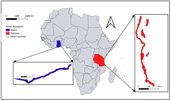
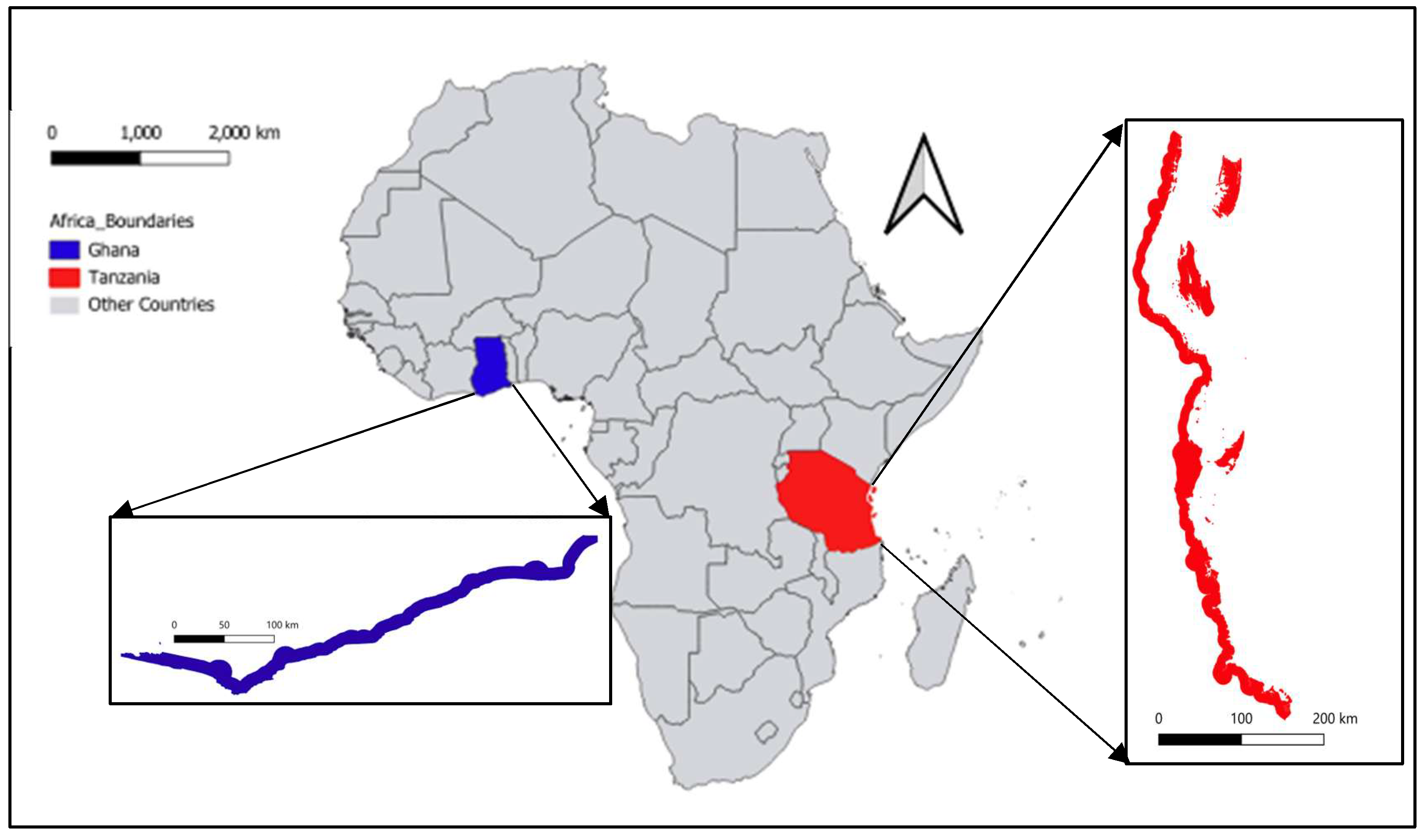
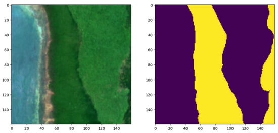
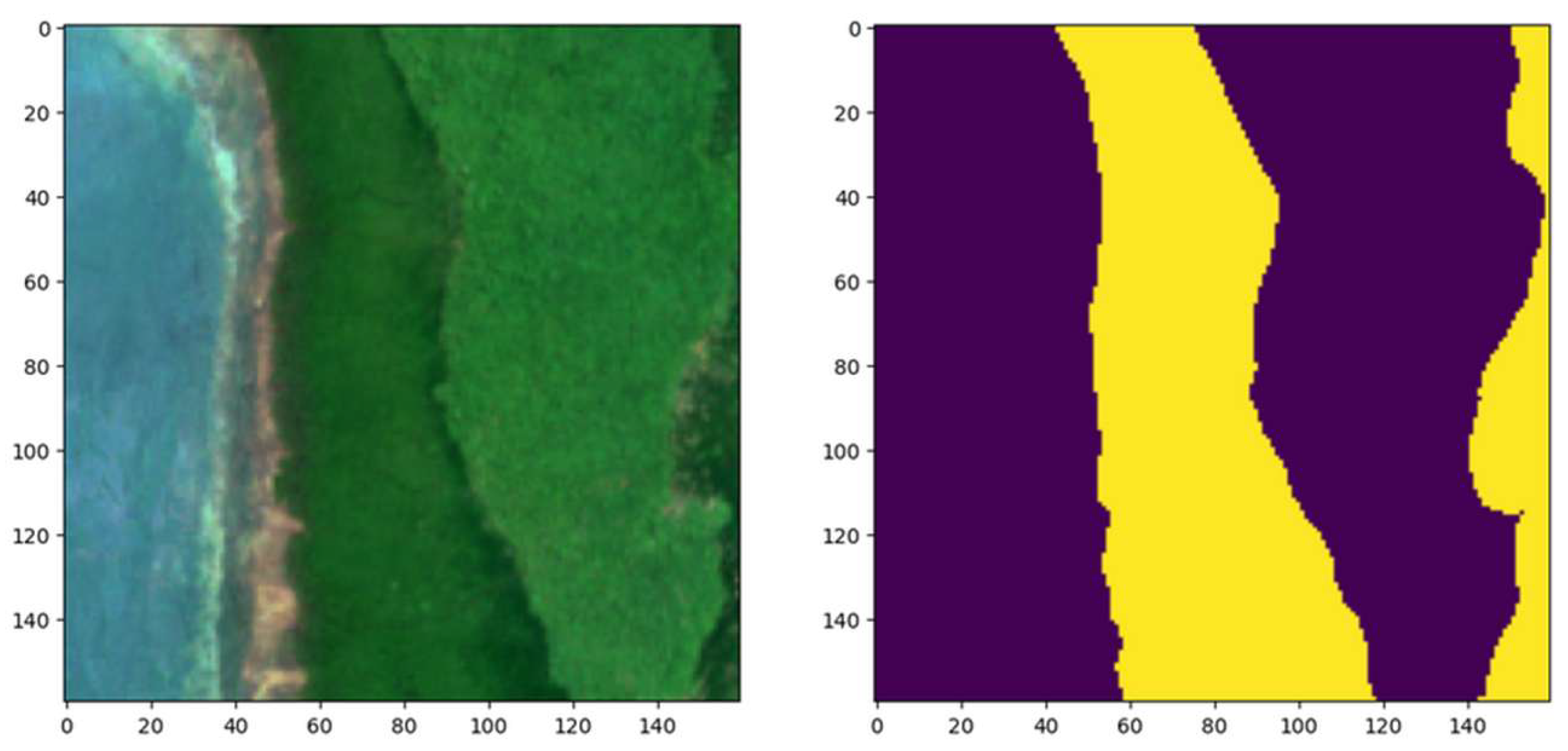
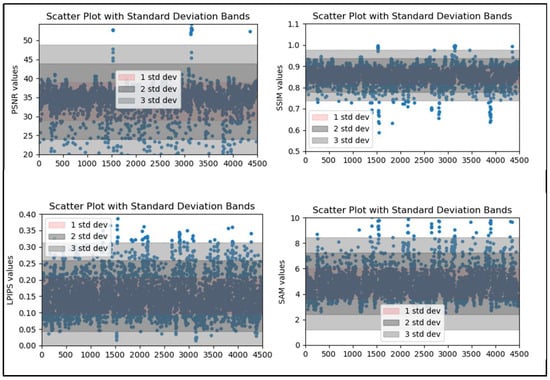
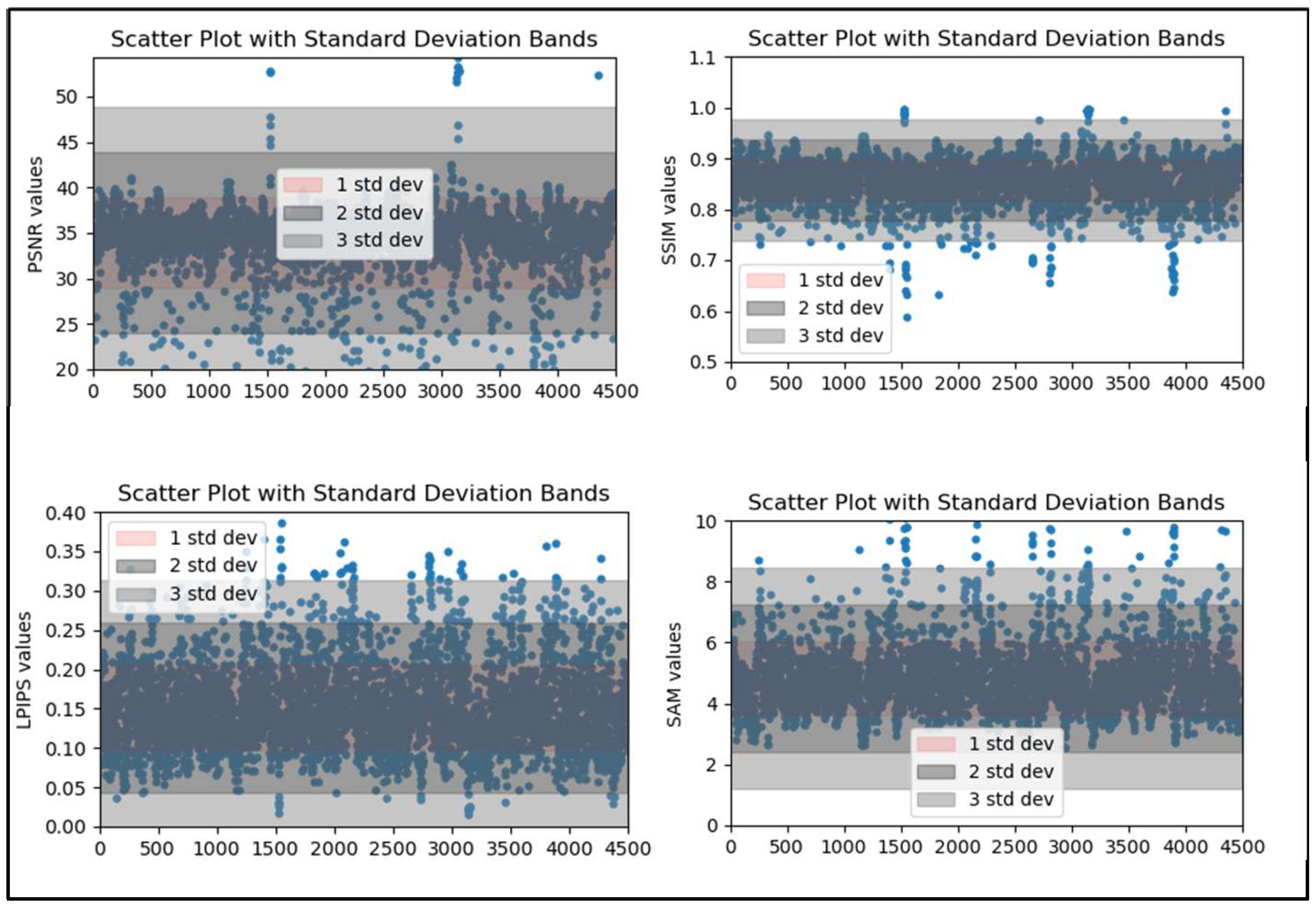
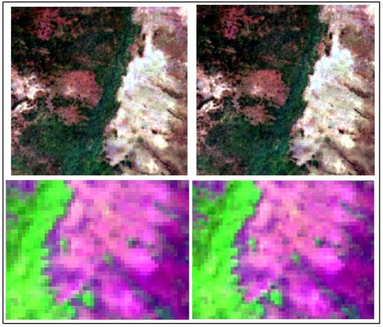
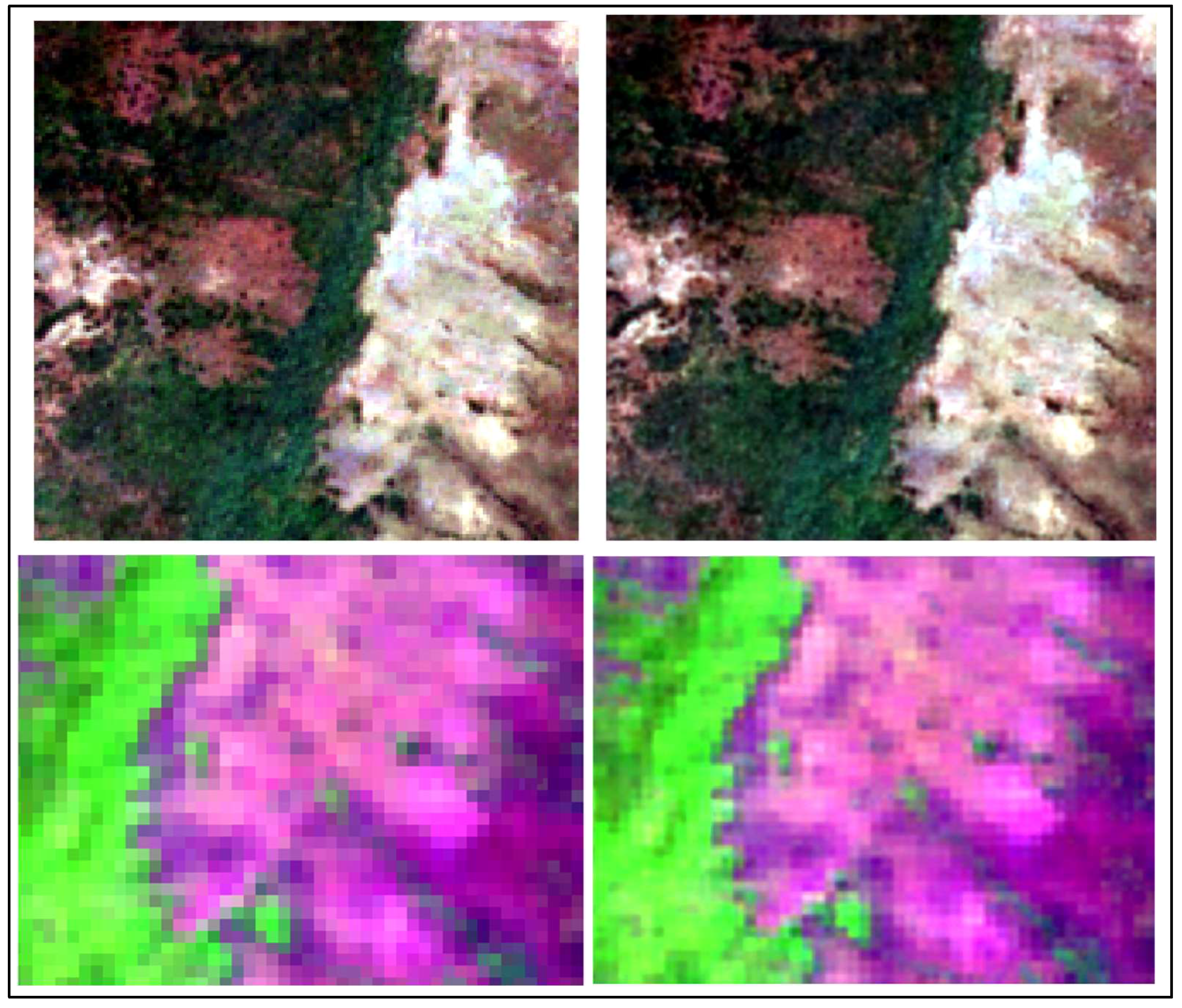
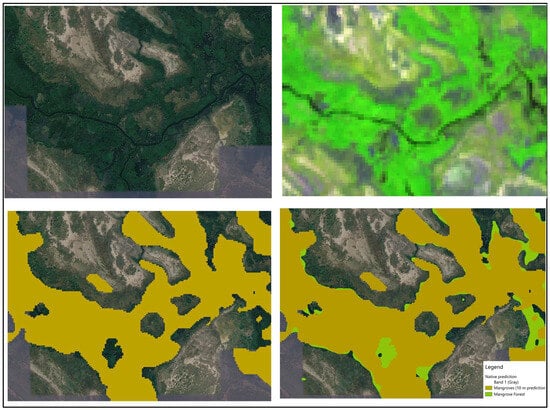
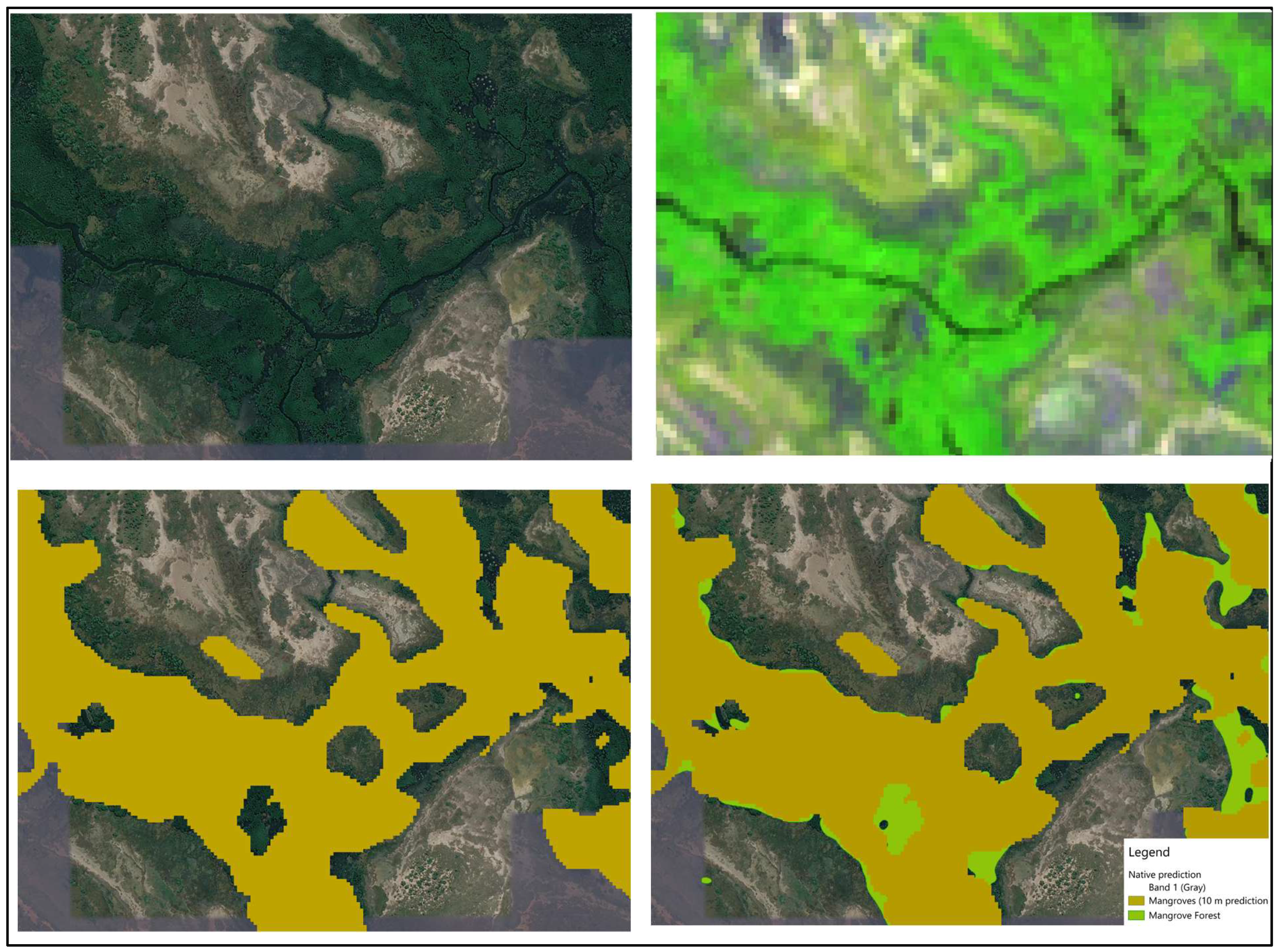
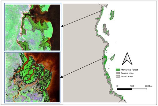
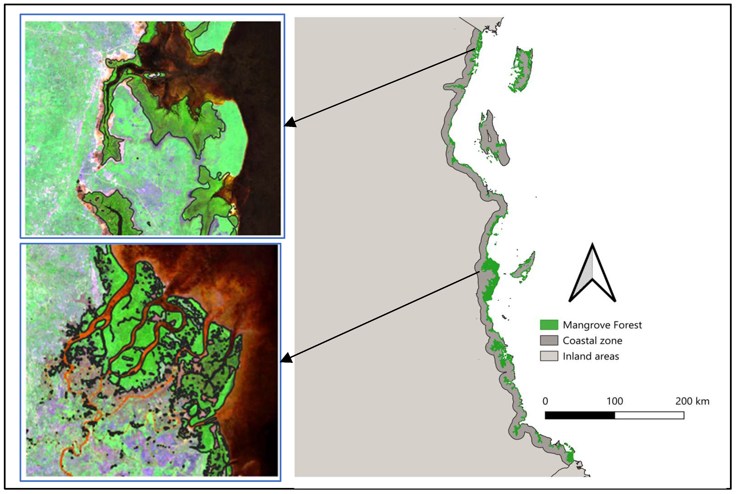
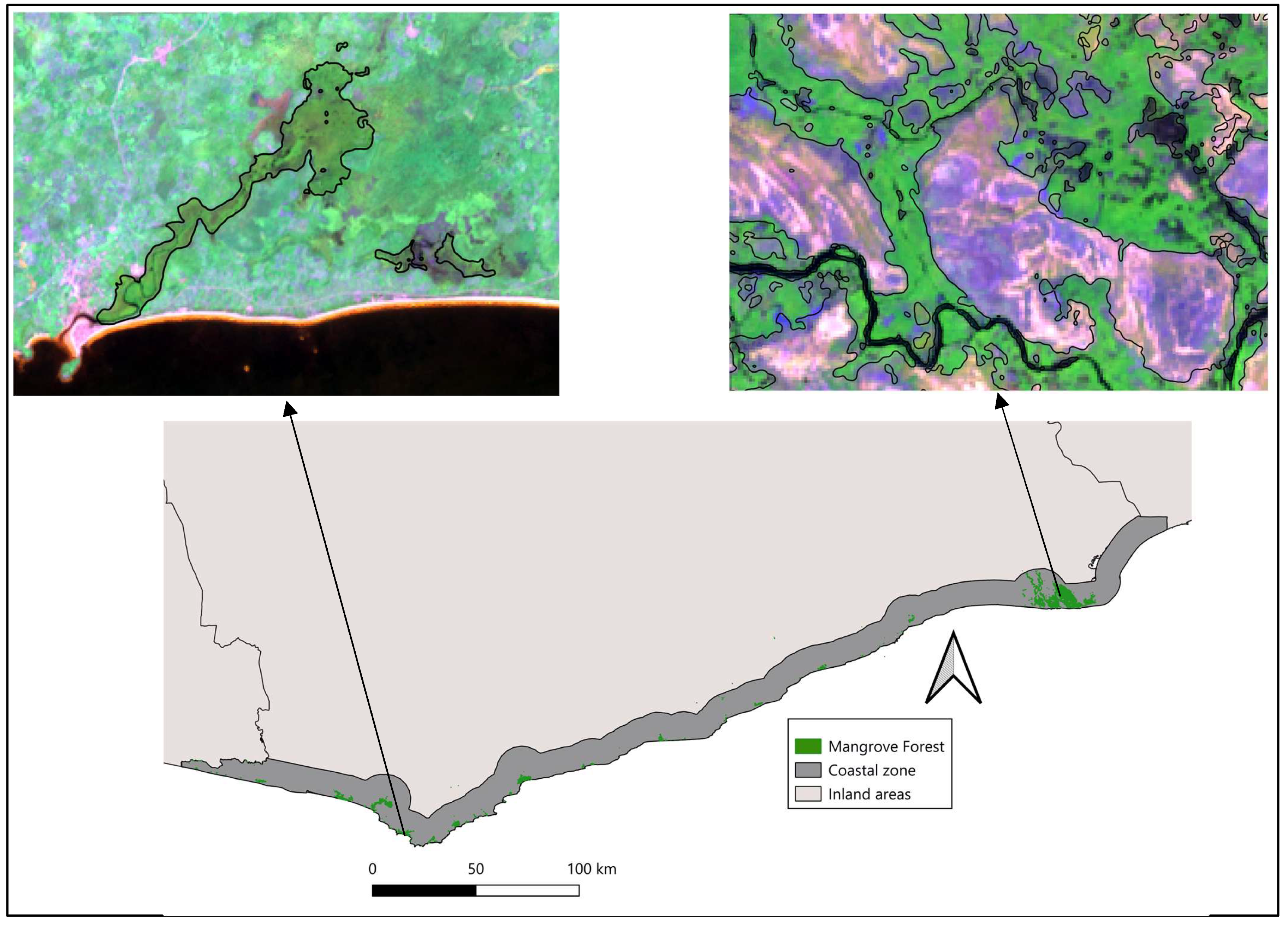
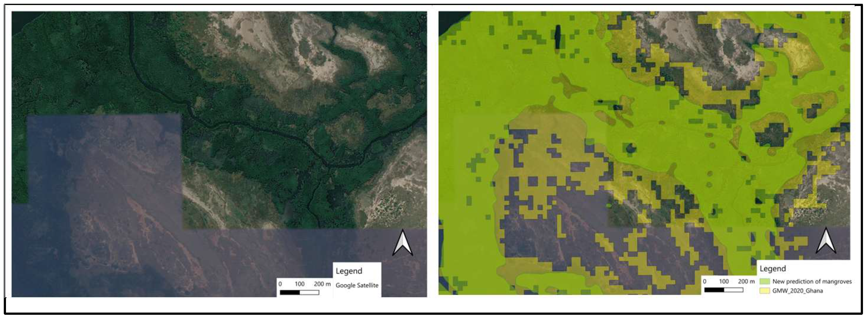

Disclaimer/Publisher’s Note: The statements, opinions and data contained in all publications are solely those of the individual author(s) and contributor(s) and not of MDPI and/or the editor(s). MDPI and/or the editor(s) disclaim responsibility for any injury to people or property resulting from any ideas, methods, instructions or products referred to in the content. |
© 2026 by the authors. Licensee MDPI, Basel, Switzerland. This article is an open access article distributed under the terms and conditions of the Creative Commons Attribution (CC BY) license.