A Deep Learning-Based Pipeline for Detecting Rip Currents from Satellite Imagery

Highlights

What are the main findings?

• A deep learning-based pipeline was developed for detecting rip currents from satellite imagery and demonstrated efficacy in locating rip occurrences within complex coastal scenes.
• A new image dataset featuring rip currents as small objects in far-view satellite images was established, expanding available resources for rip current research.

What are the implications of the main findings?

• Reliable detection of rip currents using satellite imagery can provide valuable geospatial information for characterization and assessment of this coastal hazard.

Abstract

Detecting rip currents from satellite imagery offers valuable information for the characterization and assessment of this coastal hazard. While recent advances in deep learning have enabled automatic detection from close-view beach images, the broader geospatial context available in far-view satellite imagery has not yet been fully exploited. The main challenge lies in identifying rips as small objects within large and visually complex scenes that include both beach and non-beach areas. To address this, we proposed a detection pipeline which partitions high-resolution satellite images into small regions on which rip currents are detected using a deep learning object detection model that merges the results. The merged results are processed by applying a deep learning classification model to filter out non-beach scenes, followed by applying the detection model on augmented images to remove spurious detection. The proposed pipeline achieved an overall accuracy of 98.4%, a recall of 0.890, a precision of 0.633, and an F2 score of 0.823 on the testing dataset, demonstrating its effectiveness in locating rip currents within complex coastal scenes and its potential applicability to other regions. In addition, a new rip image dataset containing far-view satellite imagery was constructed. With the new dataset, we demonstrated a potential application of the proposed method in characterizing rip occurrences and found that rip currents tended to occur at open beaches under moderate-energy, onshore-directed waves conditions. Overall, the proposed pipeline, unlike existing near-real-time rip current monitoring systems, provides a high-accuracy offline analysis tool for rip current assessment using satellite imagery. Along with the new dataset introduced in this work, it can represent a valuable step towards expanding available resources for improving automated detection methods and rip current research.

1. Introduction

A rip current is widely known as a coastal hazard posing a severe safety threat to recreational beach users. Every year, rip current-related drowning incidents are reported globally [1]. Unsuspecting bathers, once caught in a rip current, can be quickly swept into deep water [2]. A rip current is depicted as a strong, narrow, seaward water jet with offshore-directed flow at a speed of up to 0.5–2 m/s [3]. The classic rip current flow pattern consists of feeding currents, a rip neck, and a rip head [4]. Feeding currents are converging longshore currents generated due to alongshore variations in wave breaking close to the shoreline. The rip neck originates from feeding currents and appears as a narrow flow extending through and beyond the surf zone. The rip head is the decelerated flow dissipating outside of the surf zone [3]. Typical locations of rip currents include gaps between sandbars, alongshore bar-trough system with incised rip channels, transverse bar systems (e.g., [5,6,7]), near coastal structures and headlands (e.g., [8,9,10,11]), and planar sections or alongshore uniform beaches (e.g., [12,13,14]). In view of the hazardous nature of rip currents and their variable occurrence locations, detecting rip currents at beaches is an important task for fostering waterfront safety for coastal communities.

To identify occurrences of rip currents, two approaches commonly used are direct measurements of nearshore velocities and indirect visualization of rip-induced water surface features. Direct measurements are conducted using in situ velocimeters (e.g., [6,9,15]) and Lagrangian drifters (e.g., [16,17]), from which rip currents are identified as the offshore-directed flows in measured velocity time series or flow fields. Field measurements allow for direct observation of rip current velocities, but this approach is labor- and instrument-intensive, and the spatial coverage of a field campaign is typically limited to a specific beach or a small nearshore region. On the other hand, indirect visual identification is based on discerning rip-induced features that are distinguishable from the surrounding water. Such features include dark, calm regions between breaking waves [18] and offshore-directed sediment-laden or bubble plumes [19]. Manual visual inspection by trained lifeguards at patrolled beaches has long been used to detect rip occurrences [20]. Recently, image processing techniques have also been increasingly employed to assist visual detection. For example, time-averaged images showing bright breaking wave regions, which are a proxy for the presence of shallow bars, have been used to monitor morphological evolutions of rip channels (e.g., [21]). Color thresholding has been applied on images converted to the hue–saturation–value (HSV) color space to detect rip-induced sediment plumes [22,23,24]. In addition, optical flow algorithms and PIV methods have also been developed to identify offshore-directed fast water jets from videos [25,26,27,28,29]. Despite limitations such as their applicability to rip currents only with visible sediment plumes (e.g., [24]) or the long processing times required for video data (e.g., [28]), image processing techniques have demonstrated the potential for automated rip current detection from optical imagery.

Recent advances in machine learning have provided new alternatives to manual identification and traditional image processing techniques for rip current detection from optical images. The feasibility of machine learning-based rip detection was first demonstrated using time-averaged images by Maryan et al. [30], and subsequently extended to still images and videos by De Silva et al. [31] by framing rip detection as an object detection task. Specifically, Maryan et al. [30] focused on rip channel detection by comparing machine learning-based object detection algorithms, including two convolutional neural networks (MobileNet and Inception). De Silva et al. [31], in contrast, targeted rip currents associated with breaking waves using a region-based CNN (Faster R-CNN) with a custom designed temporal aggregation stage. In addition, De Silva et al. [31] established a rip image dataset containing high-resolution aerial images of rip currents along with rip-absent beach scenes, which has since been widely used in subsequent studies (e.g., [32,33,34]). Building on these early feasibility studies, later work focused on improving model architectures specifically tailored for rip current detection. For example, Rashid et al. [35,36] developed RipDet and its improved version RipDet+ based on the YOLOv3-tiny architecture, incorporating residual mapping to achieve accurate rip detection with a small number of training samples. Zhu et al. [34] developed YOLO-Rip, a YOLOv5s-based model with a joint dilated convolutional module and a parameter-free attention mechanism, to better capture rip current features, along with an expanded rip image dataset. In most of the aforementioned approaches, rip currents are represented using rectangular bounding boxes, which can limit the precise localization of their inherently amorphous structures. To address this, Rampal et al. [32] integrated a MobileNet classifier with an interpretable AI tool Grad-CAM (gradient-weighted class activation maps), framing rip current detection as a semi-supervised task based on image classification and saliency mapping. Alternatively, Dumitriu et al. [33] adopted a segmentation-based approach, developing a YOLOv8-based benchmark model and a polygonally annotated rip current dataset to enable more detailed representation. More recent studies have increasingly emphasized model explainability and efficiency for real-time applications. For instance, Choi et al. [37] applied the XAI tool Eigen-CAM to interpret detection results from Faster R-CNN, YOLOv5, and YOLOv8 models with a novel rip current dataset containing more than 100,000 coastline images. Khan et al. [38] developed RipScout, a drone-based real-time rip detection and data acquisition system, demonstrating efficient detection under a resource-constrained environment. Overall, deep learning-based rip detection has undergone rapid development, progressing from initial feasibility demonstrations to increasingly specialized model designs, and more recently toward enhanced interpretability and efficiency.

Despite these advances, one notable limitation remaining in deep learning-based rip detection is the lack of geospatial quantification for detected rip currents. Most existing deep learning-based models are trained on non-rectified images captured from various perspectives without explicit georeferenced information. Although this flexibility enhances convenience, it also constrains the applicability of detection results in tasks where georeferenced locations or spatial dimensions (e.g., width, length) are needed. Satellite imagery, which inherently contains georeferenced information and has been employed in rip current characterization and assessment studies [39,40,41], could address the limitation in geospatial quantification. However, the small size of rip currents (~10–100 m) relative to the spatial scale of natural beaches (~1–10 km) would impose a challenge of automatically detecting small objects within a large field of view. Images used in existing rip detection studies are mostly close-view beach scenes. For examples, the dataset created by de Silva et al. [31] included a large number of images sourced from Google Earth, but these images were cropped into sectioned beach scenes where rip currents appear as large, noticeable targets [34]. In recent years, various small object detection techniques have been developed, such as multi-scale feature extraction and fusion, attention mechanisms, super-resolution techniques, data augmentation, and transfer learning [42,43]. While these techniques aim to improve model architecture and training strategies, one important challenge remains: the high computational overhead associated with training on large datasets of high-resolution images. In the context of far-view satellite imagery that typically spans kilometer-scale spatial extents at sub-meter resolution, this would either require an excessively large and computationally expensive model or substantial image downscaling, which could obscure small yet critical features of rip currents. Therefore, it is difficult to directly apply the existing small object detection methods to far-view satellite images at native resolution. To our knowledge, identification of rip currents from satellite imagery has so far relied on manual visualization or non-AI approaches [44]. To address this challenge, an alternative approach based on a partition–merge perspective is proposed in this study.

The purpose of this paper is to develop a deep learning-based framework for detecting small rip current objects from satellite imagery. The contributions of this study are twofold. First, we present a rip current detection pipeline designed to address the challenge of detecting rip currents as small objects within far-view satellite images, which often contain visually complex scenes spanning both beach and non-beach areas. Second, we extend available rip current image resources by establishing a new dataset featuring rip currents in far-view satellite imagery. Together, the proposed method and dataset may offer a useful basis for extracting geospatial information on rip currents from satellite images, supporting future efforts in characterizing and assessing rip current hazards along coastal regions.

2. Materials and Methods

2.1. Detection Pipeline

In this study, a detection pipeline was proposed to address the challenge of detecting small rip current objects from satellite imagery. The basic workflow of the proposed pipeline, as illustrated in Figure 1, consists of (i) partitioning a large satellite image into small regions, (ii) performing rip current detection on the partitioned images, (iii) merging the results to form candidate regions, (iv) applying beach classification to filter out non- beach scenes, (v) augmenting beach scene images and performing rip current detection on the augmented images, and (vi) determining the final positions of rip currents in the original images.

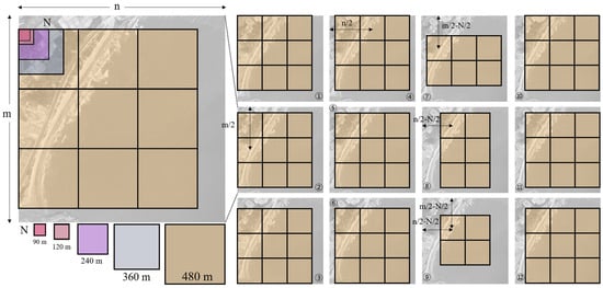
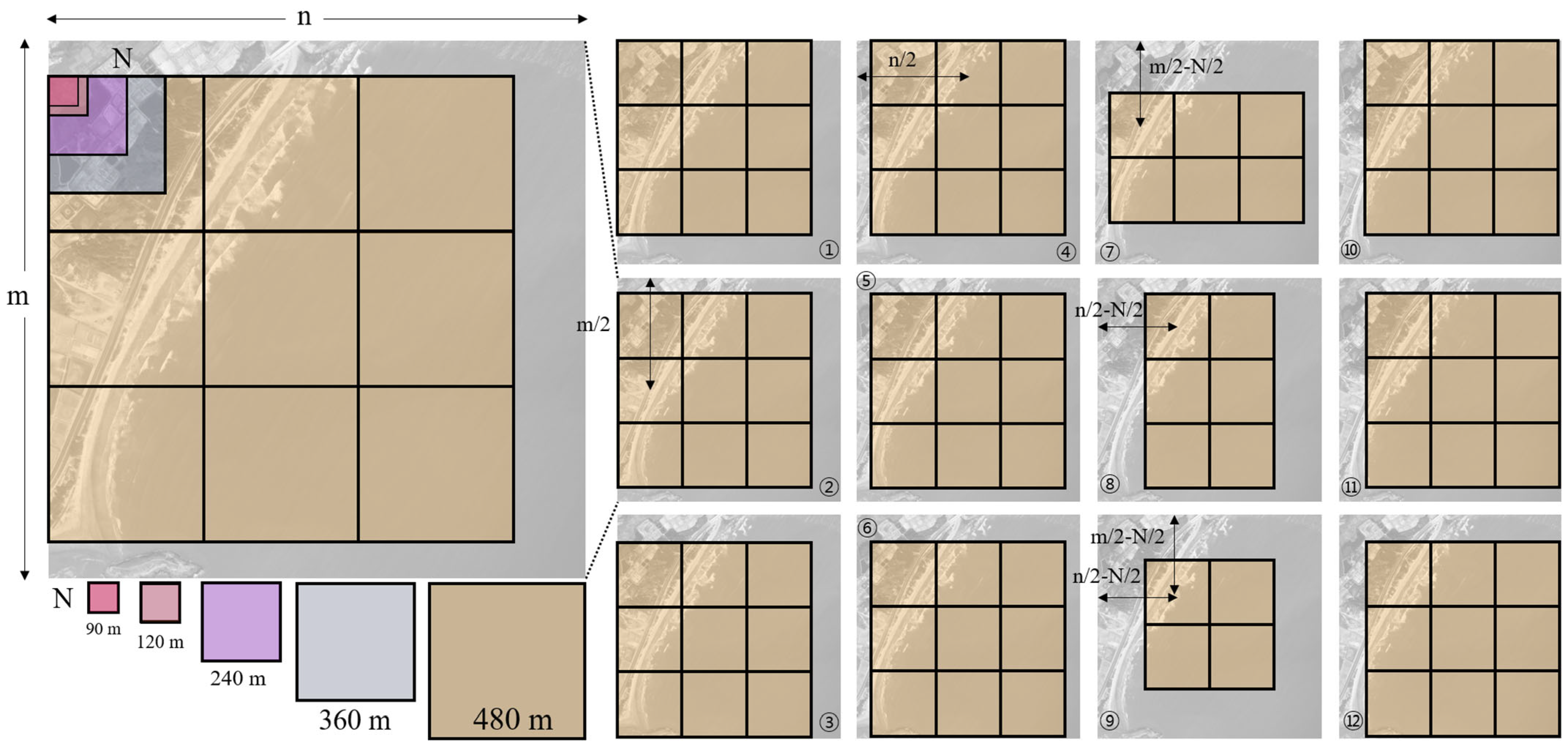
The first step is to partition a large satellite image into small square regions. Since object detection models typically operate on a fixed input size, directly resizing a large image could cause small rip current objects to lose important visual features. The partition step was therefore designed to preserve those features. The partition window size and partition scheme are two major considerations. As too-small or poorly partitioned regions may fail to capture the complete rip current structure along with enough surrounding water to provide visual contrast needed for reliable detection, a range of window sizes and partition schemes are used. Specifically, the pixel size (N) of the partition window is calculated as N = W/r, where r (in meters per pixel) is the pixel resolution of satellite imagery and W (in meters) is the actual spatial coverage of a partitioned region. Based on observed rip currents that typically have spatial dimensions on the order of 10–100 m [20,23], W values of 90 m, 120 m, 240 m, 360 m, and 480 m were used in this study, and the corresponding pixel size N was calculated. Five window sizes were selected to provide progressive scaling to represent the range of field-observed rip current sizes, while also incorporating sufficient surrounding context for rip detection. These values were additionally chosen to be compatible with the typical spatial resolutions of the georeferenced imagery used (0.3 m, 0.6 m, and 1.2 m), ensuring that the corresponding window dimensions in pixels are integers. The partition scheme divides the image into a set of contiguous, non-overlapping windows by selecting a starting position (P_m, P_n) at a corner or along an edge of the image and then tiling the remaining areas. Because the window size (N) does not evenly divide the height (m) and width (n) of the original image (in pixels), certain columns and rows along the opposite boarders may remain uncovered in a single partition. A set of different starting positions was applied to ensure that all regions are included across partitions. Figure 2 shows the 12 partition schemes with the different starting positions used in this study. Note that (P_m, P_n ) = (1, 1) means the left top corner of the image, and (m − N/2, 1) means the bottom left corner with the row shifted upwards by half of the window size. In short, the first step generates multiple small close-view images from one original far-view satellite image, and those partitioned images are to be used as the input for the rip detection model in the next step.

The second step is to perform rip current detection on the partitioned small images. The rip current detection model predicts the presence of rip currents and their bounding box locations in an image. This step is fundamentally similar to many previous works (e.g., [31,34]) and the rip detection model used in the pipeline can be any object detection model trained on rip current datasets. In this study, the YOLO11 model [45], one of the recent iterations of the YOLO (You Only Look Once) series, was employed in consideration of its good balance between efficiency and accuracy. As a single-stage object detection model, YOLO is composed of (i) a backbone, for extracting features from the original images at multiple scales, (ii) a neck, for refining and aggregating the extracted multi-scale features into a more efficient feature representation, and (iii) a detection head, for processing the feature maps from the backbone and neck and performing regression and classification to generate the final predictions of object bounding boxes and class labels. In particular, the YOLO11 architecture is highlighted by the introduction of a C3k2 (Cross Stage Partial with kernel size 2) block and SPPF (Spatial Pyramid Pooling—Fast) with a C2PSA (Convolutional block with Parallel Spatial Attention) component, which contribute to enhanced feature extraction capabilities and optimized efficiency and performance [46]. YOLO11 provides a range of model sizes to accommodate diverse deployment needs, along with pretrained models trained on the COCO dataset. In this study, the YOLO11s pretrained model was employed and further trained using a new rip current dataset established in this study. In short, the second step generates a set of predicted rip current bounding boxes using a deep learning object detection model.

In the third step, bounding boxes predicted in the partitioned images were merged to form a list of candidate rip regions. Specifically, the relative coordinates of bounding boxes in each partitioned image were mapped to their corresponding relative coordinates in the original image. Overlapping detections, determined as two bounding boxes with an intersection-over-union (IoU) greater than 0.5, were merged. Here, the IoU threshold of 0.5 was adopted as a balanced choice, as lower thresholds tend to merge spatially adjacent but distinct structures while higher thresholds may increase subsequent processing time by retaining duplicate detections of the same structure. A sensitivity test further indicates that the merging outcome is not strongly dependent on the exact threshold value, as the number of merged boxes in the testing dataset images varied by less than 10% relative to the IoU = 0.5 case when the threshold was set between 0.3 and 0.7. The merged box is defined as the minimum outer bounding box that fully encloses the two overlapping boxes. It is important to note that all predictions in the partitioned images are considered valid to be merged to form a rip current candidate region in this step. Nevertheless, the partitioned images are not ideal beach scenes where a rip current is either clearly visible at the center of the image or entirely absent. In many cases, a rip current becomes only partially visible because the partitioning process may cut the visual cues in half. In other cases, intense breaking waves adjacent to a rip current may produce color contrasting patterns that resemble the appearance of a rip current. Moreover, images partitioned from far-view satellite images contain a large number of non-beach scenes of land or offshore water, including buildings, roads, farmland, inland water bodies, rocky islands, and boat wakes. The presence of such visually complex and diverse features increases the likelihood of spurious detections, and additional procedures are needed. In short, the third step merges the prediction result and forms a list of candidate regions of rip currents which are to be further checked in the next steps.

In the fourth step, the merged candidate regions were checked using a beach classifier and those classified as “non-beach” scenes were removed from the candidate list. The input to the beach classifier is an image of a cropped candidate region. To avoid nonrealistic small regions, the cropped image is required to be at least 90 m in its actual dimension, consistent with the smallest partitioned image size. An image is classified as either a beach scene or a non-beach scene. The beach images primarily contain scenes of shoreline and surf zones where rip currents can possibly occur, while the non-beach images are mostly scenes of land and offshore water where no visual signature of wave breaking is observed. The YOLO11 classification model, a variant of the EfficientNet architecture with C3k2 and C2PSA components, was adopted here. YOLO11s-cls pretrained on the ImageNet dataset was employed and further trained using images from the new dataset in this study. In short, the fourth step filters out spurious non-beach scenes from the merged candidate regions using a deep learning-based image classification model.

The fifth step is to perform rip current detection on a set of augmented images for those candidate regions classified as beach scenes. The augmented images were generated by cropping squares from the original satellite image at various scales so that the candidate region appears at different proportions of the square patches. The largest crop was chosen so that the candidate region occupies about 30 percent of the crop, and the smallest crop was chosen so that it occupies about 90 percent. This corresponds to square crop sizes of max(w, h)/0.3 for the largest scale and max(w, h)/0.9 for the smallest scale, where max(w, h) is the pixel dimension of the longer side for the rectangular candidate region in the original image. Additional crop sizes were generated between these two limits, and a fixed increment of p = 64 pixels was used in this study. The same YOLO11 detection model trained in the second step was then applied to all augmented images. If the predicted bounding box has an IoU greater than 0.5 with the candidate region, it is counted as a valid detection. If the number of valid detections exceeds half of the number of augmented images, the candidate region is determined as a final rip current detection. In short, the fifth step double-checks rip detections by applying the detection model on augmented images, and the final detection results are determined based on these outcomes.

2.2. Dataset

The three data sources of high-resolution satellite imagery used for training the detection and classification models and for evaluating the proposed detection pipeline are summarized in

Table 1. Three sources of high-resolution satellite imagery for rip current detection.

Source	1	2	3
	de Silva et al. [31]	Google Earth Historical Imagery	ESRI World Imagery
Images	2440	307	387
Rip	1740	257	40
Non-rip	700	50	347
Acquisition Time	-	2005–2024	2008–2021
Beach Locations	-	21 beaches along the coastal region of Guangdong Province	71 beaches in the Guangdong–Hong Kong–Macao Greater Bay Area
Usage	Training the rip detector	Training the rip detector and beach classifier	Testing the rip detection pipeline

. The first data source is the open-access rip current dataset developed by de Silva et al. [31], which contains 1740 images of rip currents and 700 images with no rip. Images in this dataset were sourced from Google Earth high-resolution aerial images and cropped into smaller beach scenes, where close-view rip currents appear as large objects near the image center. Since this dataset mainly contains unambiguous examples that clearly depict the fundamental morphological features of rip currents, it was used for training the rip detector. The second data source is Google Earth Historical Imagery. A total of 307 satellite images captured during the period of 2005–2024 were obtained for 19 beaches along the coastal region of Guangdong Province, China (see

Table A1. List of satellite imagery sites along coastal region of Guangdong Province.

	Site Name	Latitude Range		Longitude Range		Image Acquisition Time
1	DaJiaoWan	21.550	21.567	111.833	111.850	2014-10, 2019-09, 2021-05, 2021-09, 2024-10
2	GaoLan Beach	21.900	21.917	113.267	113.283	2010-10, 2013-11, 2014-12, 2015-01, 2018-01, 2021-02, 2022-05, 2024-01
		21.850	21.900	113.233	113.300	2022-05
3	GuangAoWan	23.167	23.267	116.717	116.817	2012-10, 2012-11, 2013-01, 2014-10, 2014-11, 2014-12, 2016-08, 2018-05, 2018-12
		23.217	23.250	116.700	116.750	2012-08, 2012-11, 2013-09, 2014-01, 2014-03, 2014-09, 2014-11, 2016-02, 2016-08, 2019-01, 2019-09, 2019-10, 2020-09
		23.183	23.233	116.667	116.717	2010-08, 2011-12, 2012-08, 2012-11, 2012-12, 2013-01, 2013-09, 2014-03, 2014-11, 2015-03, 2016-02, 2016-09, 2017-01, 2017-10, 2017-12, 2018-05, 2018-12, 2019-09, 2019-10, 2020-09, 2022-09
		23.167	23.200	116.650	116.683	2011-12, 2012-11, 2013-01, 2013-09, 2014-10, 2014-11, 2014-12, 2015-03, 2016-02, 2016-09, 2017-01, 2017-10, 2017-11, 2017-12, 2018-01, 2018-10, 2019-10, 2022-09, 2024-01
4	HaiMenWan	23.083	23.200	116.533	116.650	2009-01, 2012-08, 2012-11, 2014-09, 2014-10, 2014-11, 2014-12, 2016-02, 2016-09, 2017-10, 2017-12, 2018-01, 2018-02, 2018-10, 2018-12, 2020-04
		23.017	23.133	116.500	116.617	2010-12, 2012-09, 2013-01, 2013-09, 2014-06, 2015-03, 2016-03, 2016-09, 2017-06, 2017-10, 2017-11, 2017-12, 2018-03, 2019-10, 2020-04, 2020-09
5	HeBeiWan	21.483	21.533	111.550	111.617	2014-01, 2014-10, 2017-01, 2017-10, 2019-09, 2021-03, 2021-09
6	HouMenWan	22.767	22.817	115.100	115.133	2012-10, 2017-01, 2017-02, 2018-11, 2022-08, 2022-10
7	HuDongWan	22.767	22.800	115.900	115.933	2014-11, 2016-12, 2017-11, 2018-01, 2020-01, 2020-02, 2021-08, 2022-04, 2022-12, 2023-02
8	JiaZiWan	22.767	22.850	116.000	116.083	2006-04, 2010-12, 2011-02, 2013-01, 2014-01, 2016-12, 2017-11, 2018-01, 2020-04, 2022-01, 2022-03, 2022-04, 2024-08
9	JieShiWan	22.800	22.867	115.583	115.650	2013-01, 2020-07, 2020-11, 2022-10
		22.833	22.867	115.667	115.700	2012-09, 2013-01, 2018-09, 2018-10, 2020-11
		22.783	22.800	115.550	115.567	2015-01, 2016-03, 2019-03, 2020-11, 2021-04
		22.783	22.783	115.533	115.550	2015-01
		22.767	22.783	115.533	115.550	2013-01, 2015-01, 2016-12, 2019-03, 2020-11, 2021-04, 2022-10
		22.683	22.750	115.567	115.617	2013-01, 2015-01, 2016-02, 2016-03, 2017-08, 2018-09, 2018-10, 2021-04, 2022-01, 2024-10
		22.633	22.700	115.533	115.600	2013-01, 2014-01, 2016-02, 2016-03, 2019-08, 2021-04, 2022-01, 2024-10
		22.650	22.667	115.517	115.550	2018-03, 2018-10, 2020-04, 2023-10
		22.667	22.683	115.467	115.500	2014-01, 2016-03, 2016-12, 2018-10, 202-210
		22.650	22.700	115.417	115.467	2005-11, 2013-01, 2014-09, 2015-08, 2016-03, 2016-12, 2018-10, 2022-06, 2022-10
		22.633	22.700	115.317	115.400	2018-03, 2021-11, 2022-10
10	JingHaiWan	22.950	23.000	116.500	116.550	2010-12, 2012-08, 2012-09, 2014-06, 2016-03, 2017-04, 2017-10, 2017-12, 2018-03, 2018-12, 2019-10, 2020-01, 2021-01
11	LiBianWan	21.633	21.633	112.000	112.017	2014-10, 2021-11
12	NanWan	21.833	21.850	113.133	113.167	2010-10, 2012-10, 2013-12, 2014-12, 2015-01, 2017-12, 2019-08, 2024-01
13	PingHaiWan	22.567	22.600	114.850	114.883	2011-01, 2014-10, 2017-10, 2019-07, 2019-11
		22.567	22.600	114.817	114.850	2008-09, 2013-10, 2014-07, 2014-10, 2017-01, 2017-02, 2017-10, 2019-07, 2019-10, 2020-12
14	RuDongHe	21.483	21.517	111.383	111.417	2014-10, 2017-03, 2017-10
		21.467	21.500	111.333	111.383	2013-03, 2014-01, 2014-11, 2017-03, 2017-04, 2017-07, 2018-03, 2020-01, 2021-08, 2021-10
		21.433	21.467	111.317	111.350	2011-12, 2013-03, 2014-01, 2014-10, 2016-10, 2017-03, 2017-04, 2017-07, 2017-10, 2018-03, 2020-01, 2021-08, 2021-12
15	ShanWeiWan	22.750	22.800	115.267	115.317	2013-01, 2015-01, 2015-08, 2017-02, 2017-10, 2017-12, 2022-06, 2024-10
16	ShenQuanWan	22.900	22.967	116.233	116.317	2008-12, 2011-12, 2013-01, 2015-09, 2017-09, 2017-10, 2017-12, 2018-07, 2018-10, 2021-01
17	ShuangGuanWan	21.567	21.633	111.717	111.783	2014-01, 2021-03
		21.550	21.600	111.667	111.717	2016-11, 2017-01
18	WangCunWan	21.383	21.417	110.917	110.950	2010-09, 2017-10, 2021-07
		21.367	21.400	110.883	110.917	2014-11, 2015-01, 2019-10, 2020-11, 2021-07
19	XiaoMoWan	22.750	22.783	115.050	115.083	2014-10, 2015-10, 2017-01, 2017-02, 2018-11, 2020-11, 2021-02, 2021-11

). These far-view images were cropped into smaller regions of various sizes to represent different scales. The cropped images contain a wide range of scenes, including both beach regions where rip currents can be present and non-beach regions such as offshore water and lands, and thus were used for training both the rip detector and beach classifier. The third data source is the ESRI World Imagery dataset, which provides georeferenced satellite images with spatial resolutions ranging from 0.3 m to 1.2 m per pixel. A total of 387 satellite images captured during 2008 and 2021 were obtained for 71 beaches in the Guangdong–Hong Kong–Macao Greater Bay Area (see

Table A2. List of high-resolution satellite imagery sites in Guangdong–Hong Kong–Macao Greater Bay Area.

	Site Name	Latitude Range		Longitude Range		Image Acquisition Date
1	BengTanWan	21.727	21.736	112.381	112.391	2012-08-24, 2013-01-14, 2020-10-21
2	BiJiaWan	22.592	22.598	114.757	114.763	2008-05-15, 2013-10-24, 2017-06-23, 2019-11-11, 2021-01-19
3	CaoTangWan	21.719	21.725	112.348	112.354	2012-08-24, 2013-01-14, 2017-03-27, 2018-09-29, 2020-10-21, 2022-04-06
4	ChangShaTou	22.589	22.604	114.773	114.790	2008-05-15, 2013-10-24, 2019-11-11, 2021-01-19
5	ChangShaTou_West	22.592	22.599	114.763	114.771	2008-05-15, 2013-10-24, 2017-06-23, 2019-11-11, 2021-01-19, 2021-05-18
6	ChongKouWan	21.997	22.007	113.337	113.347	2010-11-14, 2014-12-13, 2018-01-15, 2021-02-15, 2021-12-05, 2022-10-14, 2023-10-13
7	DaHaiWan	21.860	21.891	112.687	112.721	2010-10-23, 2012-11-13
8	DaJinDao	21.849	21.862	113.018	113.032	2010-07-13, 2015-08-09, 2021-02-02, 2021-10-06
9	DaLangWan	21.886	21.891	112.874	112.887	2010-10-23, 2015-08-25, 2019-10-29, 2023-02-28
10	DaShaWan	21.934	21.940	113.272	113.279	2008-01-15, 2014-12-13, 2017-11-01, 2019-09-29, 2019-12-02, 2021-10-06, 2023-07-15
11	DaWuWan	22.366	22.370	113.619	113.624	2015-10-21, 2017-11-01, 2019-01-26, 2019-12-06, 2022-03-02, 2023-04-30
12	DaXiaoMeiSha	22.587	22.606	114.298	114.330	2010-11-03, 2015-01-01, 2021-11-08
13	DaYaWan	22.766	22.780	114.642	114.679	2008-05-15, 2013-10-24, 2018-05-14, 2019-11-11, 2020-12-27
14	DongHeCun	22.630	22.644	114.919	114.934	2008-05-15, 2013-10-24, 2021-01-26, 2023-02-23
15	DongShanHai	22.574	22.626	114.897	114.922	2008-05-15, 2013-10-24, 2021-01-26, 2023-02-23
16	DongYongBeach	22.488	22.495	114.577	114.584	2008-05-15, 2011-08-15, 2018-05-14, 2018-10-30, 2020-01-15, 2021-03-25, 2021-11-08
17	FeiShaWan	21.912	21.919	113.279	113.287	2014-12-13, 2017-11-01, 2019-09-29, 2019-11-24, 2021-10-06, 2023-07-15
18	GangKouZhen	22.546	22.555	114.886	114.896	2008-05-15, 2013-10-24, 2017-10-25, 2021-01-26, 2023-02-23
19	GaoYangWei	22.644	22.659	114.927	114.944	2013-10-24, 2021-01-26
20	GuanHuBeach	22.594	22.609	114.412	114.428	2008-05-15, 2015-04-15, 2021-11-08
21	HK-DaLangWan	22.244	22.248	114.245	114.249	2010-12-06, 2014-10-12, 2017-01-21, 2019-12-14, 2021-10-11, 2022-09-08
22	HK-ShangChangShaBeach	22.225	22.236	113.934	113.958	2010-12-06, 2016-07-29, 2019-09-22, 2020-03-16, 2022-03-02, 2025-01-10
23	HaiBinBeach	22.254	22.261	113.584	113.591	2010-11-11, 2015-10-21, 2017-11-01, 2019-01-26, 2019-12-06, 2022-09-13, 2024-06-27
24	HeBaoDao_East	21.856	21.858	113.179	113.182	2008-01-15, 2010-10-23, 2017-11-01, 2018-10-05, 2020-06-12
25	HeBaoDao_South	21.846	21.860	113.145	113.173	2008-01-15, 2015-08-09, 2018-10-05, 2020-06-12
26	HeiShaWanBeach	21.861	21.875	112.927	112.942	2010-10-23, 2015-08-25, 2019-10-29, 2021-07-23, 2023-02-28
27	HengShanDao	22.247	22.250	113.596	113.599	2015-10-21, 2017-11-01, 2019-01-26, 2019-12-06, 2022-09-13, 2024-06-27
28	HuangBuZhen	22.665	22.674	114.953	114.962	2010-11-25, 2013-10-24, 2017-02-16, 2021-01-26, 2022-12-09
29	HuangHuaWan	21.704	21.710	112.300	112.308	2012-08-24, 2013-01-14, 2017-09-22, 2020-10-21, 2022-04-06
30	HuiDongXian	22.696	22.707	114.995	115.006	2010-11-25, 2013-10-29, 2017-02-16, 2021-02-14, 2021-11-21, 2022-12-09
31	HuiDongXian_East	22.702	22.709	115.013	115.021	2010-11-25, 2013-10-29, 2017-02-16, 2021-02-14, 2021-11-21, 2022-12-09
32	JiaoChangWei	22.581	22.596	114.498	114.514	2008-05-15, 2008-10-30, 2013-11-15, 2021-02-02, 2021-12-05
33	JiaoChangWei_South	22.567	22.581	114.499	114.502	2008-05-15, 2013-11-15, 2018-03-12, 2018-10-30, 2021-02-02, 2021-12-05, 2022-05-03
34	JiaoWan	21.854	21.857	112.899	112.903	2010-10-23, 2015-08-25, 2019-10-29, 2023-02-28
35	JinHaiWan	22.629	22.653	114.730	114.747	2008-05-15, 2013-10-24, 2017-06-23, 2019-11-11, 2021-01-19
36	JinShaWanBeach	22.567	22.572	114.437	114.460	2008-05-15, 2014-04-05, 2016-07-16, 2018-10-30, 2021-02-02, 2021-12-05, 2022-09-16, 2024-01-07, 2025-01-10
37	JinShaWan	21.996	22.011	113.373	113.401	2010-11-14, 2018-01-15, 2019-09-23, 2021-02-15, 2021-12-05, 2022-10-14, 2023-10-13
38	JingShanParkBeach	22.263	22.274	113.575	113.587	2015-10-21, 2017-11-01, 2019-01-26, 2019-12-06, 2022-09-13, 2023-07-15, 2024-06-27
39	JuDiaoShaBeach	22.558	22.563	114.548	114.553	2008-05-15, 2013-11-15, 2018-03-12, 2018-10-30, 2021-02-02, 2021-03-25, 2021-12-05, 2022-05-03
40	Macau-HeiBeach	22.116	22.126	113.568	113.579	2010-11-11, 2015-10-21, 2017-11-01, 2019-01-26, 2021-11-24, 2022-09-13, 2023-02-23, 2023-10-13
41	Macau-ZhuWanBeach	22.111	22.115	113.558	113.562	2011-02-04, 2015-10-21, 2017-11-01, 2019-01-26, 2021-11-24, 2022-09-13, 2023-02-23, 2023-10-13
42	MeiGuiYuanBeach	22.599	22.614	114.366	114.382	2008-05-15, 2014-10-17, 2021-11-08
43	NaYaoWan	21.723	21.731	112.354	112.378	2012-08-24, 2013-01-14, 2017-03-27, 2018-09-29, 2020-10-21, 2022-04-06
44	NanAoBeach	22.545	22.554	114.469	114.478	2008-05-15, 2014-04-05, 2016-07-16, 2018-10-30, 2021-02-02, 2021-03-25, 2021-12-05, 2022-05-03, 2024-01-07, 2025-01-10
45	PingHai	22.575	22.606	114.822	114.893	2008-05-15, 2013-10-24, 2023-02-23
46	QiAoDao_East	22.419	22.427	113.655	113.664	2010-11-11, 2015-10-21, 2016-07-29, 2019-01-26, 2021-11-24, 2022-03-02, 2023-07-15, 2023-08-21
47	QiAoDao_South	22.388	22.399	113.627	113.638	2010-11-11, 2015-10-21, 2017-11-01, 2019-01-26, 2019-12-06, 2022-03-02, 2023-04-30
48	QiAoDao_Southeast	22.403	22.412	113.642	113.652	2010-11-11, 2015-10-21, 2017-11-01, 2019-01-26, 2021-11-24, 2022-03-02, 2023-07-15, 2023-08-21
49	QinTouWan	21.876	21.893	112.958	112.983	2010-10-23, 2015-08-25, 2015-09-29, 2019-10-29, 2021-02-02, 2021-10-06, 2023-02-28
50	SanLangWan	21.907	21.911	113.274	113.279	2014-12-13, 2017-11-01, 2019-09-29, 2019-11-24, 2021-10-06, 2023-07-15
51	SanShaWan	21.707	21.714	112.314	112.322	2012-08-24, 2013-01-14, 2017-09-22, 2018-09-29, 2020-10-21, 2022-04-06
52	ShaBianCun	21.788	21.793	112.636	112.646	2010-10-23, 2011-12-29, 2021-02-17
53	ShuiShaWan	21.795	21.800	112.644	112.650	2010-10-23, 2011-12-29, 2021-02-17
54	TangJiaWanBeach	22.337	22.348	113.587	113.599	2010-11-11, 2015-10-21, 2017-11-01, 2019-01-26, 2019-12-06, 2022-09-13, 2023-04-30
55	WaYaoWan	21.800	21.825	112.645	112.652	2010-10-23, 2011-12-29, 2021-02-17
56	WanShaWan	21.847	21.856	112.671	112.682	2010-10-23, 2011-12-29, 2019-09-23, 2021-02-17
57	WangTouCun	21.758	21.769	112.569	112.610	2010-10-23, 2011-12-29, 2021-02-17
58	WangTouCun_East	21.775	21.779	112.624	112.628	2010-10-23, 2011-12-29, 2021-02-17
59	WeiJiaoWan	21.714	21.721	112.336	112.344	2012-08-24, 2013-01-14, 2017-09-22, 2018-09-29, 2020-10-21, 2022-04-06
60	XiShaWan	21.925	21.934	113.278	113.289	2008-01-15, 2014-12-13, 2017-11-01, 2019-09-29, 2019-12-02, 2021-10-06, 2023-07-15
61	XiYongBeach	22.465	22.488	114.525	114.550	2008-05-15, 2013-07-13, 2017-01-21, 2018-10-30, 2020-01-15, 2021-03-25, 2021-12-05
62	XiZhenWan	21.892	21.896	113.268	113.273	2014-12-13, 2017-11-01, 2019-09-29, 2019-12-02, 2021-10-06, 2023-07-15
63	XiaTangWan	21.712	21.721	112.324	112.333	2012-08-24, 2013-01-14, 2018-09-29, 2020-10-21, 2022-04-06
64	XiangZhouWan	22.294	22.315	113.573	113.583	2010-11-11, 2015-10-21, 2017-11-01, 2019-01-26, 2019-12-06, 2022-09-13, 2023-04-30
65	XiaoJingWan	22.776	22.800	114.684	114.710	2008-05-15, 2013-10-24, 2021-01-19
66	XiaoJingWan_East	22.779	22.788	114.724	114.733	2008-05-15, 2013-10-24, 2021-01-19
67	XinAnCun	22.594	22.600	114.793	114.800	2008-05-15, 2013-10-24, 2019-11-11, 2021-01-26
68	XunLiaoWan	22.674	22.708	114.733	114.755	2008-05-15, 2013-10-24, 2019-11-11, 2021-01-19
69	XunLiaoWan_South	22.657	22.674	114.726	114.745	2008-05-15, 2013-10-24, 2019-11-11, 2021-01-19
70	YanCongWan	22.588	22.603	114.739	114.755	2008-05-15, 2013-10-24, 2017-06-23, 2019-11-11, 2021-01-19
71	YijingWan	22.674	22.687	114.961	114.975	2010-11-25, 2013-10-29, 2017-02-16, 2021-01-26, 2022-12-09

). This dataset was not used for model training but served as an independent dataset for evaluating the performance of the proposed detection pipeline.

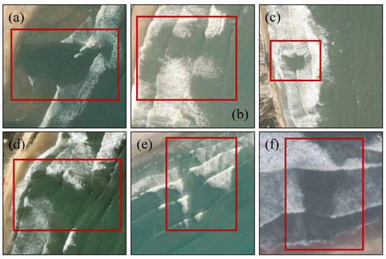
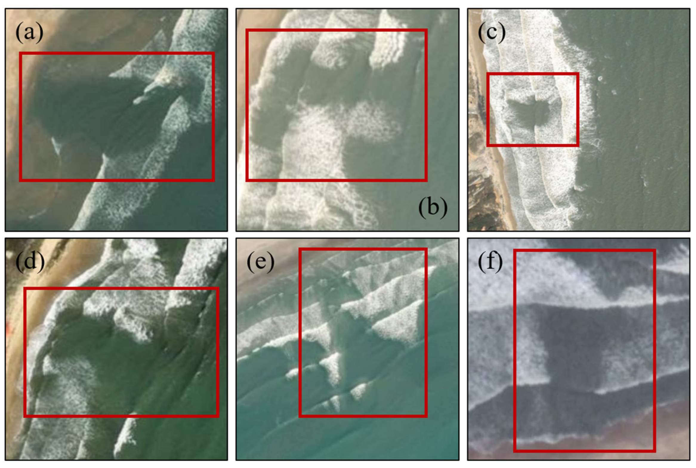
The collected satellite images (source 2, 3) were annotated to provide ground-truth labels for the detection task. Rip currents were manually annotated in the far-view satellite images using the LabelImg tool. An annotated rip current is recorded as a rectangular bounding box B = (x_c, y_c, w, h), where x_c and y_c denote the relative coordinates of the bounding box center and w and h denote its width and height, all normalized with respect to the image size. Since rip currents mostly appear as dark regions between bright, white-capping breaking waves, the surrounding water provides essential visual contrast and thus was included within the annotated bounding box, as shown in examples of Figure 3. Six morphological patterns are noted in the annotated rip currents. The “bar” type (Figure 3a) features a distinct rip channel boarded by sand bars on both sides, where visible wave breaking is often observed. The “curved” type (Figure 3b) exhibits a dark region shaped like a “C” or “L”, sometimes orientated at an oblique angle to the shoreline. The “hole” type (Figure 3c) appears as a short dark region surrounded by bright breaking waves, mostly confined within the surf zone. The “jet” type (Figure 3d) is characterized by a narrow, elongated dark region extending several wavelengths through and beyond the surf zone. The “V-shaped” type (Figure 3e) forms a calm, triangular region between breaking waves, with the width gradually increasing toward the offshore direction. Lastly, the “mix” type (Figure 3f) exhibits a dark discontinuity within the breaking wave region and contains more than one of the features of the previously described patterns (e.g., “V-shaped” and “hole” in Figure 3f). In summary, a total of 1440 rip currents were annotated in 257 far-view satellite images from the Google Earth dataset (source 2), and 91 rip currents were annotated in 40 satellite images from the ESRI dataset (source 3).

The datasets used for training the rip detector and beach classifier were constructed using images cropped from the original satellite image (source 2). For the rip detector, rip current labels which were annotated with respect to the original image size were transformed into the corresponding relative position in the cropped image. All labels were also manually checked to remove mislabeling on images where the essential visual contrast of the rip current and its surrounding water were cropped out. For the beach classifier, each cropped image was manually classified into a beach or a non-beach scene. In addition, data augmentation was applied on the training data to enhance the representation of different visual features. The three categories of image transformation employed in this study are as follows: (i) hue–saturation–value adjustment to account for different lighting conditions; (ii) image rotation, translation, and vertical/horizontal flipping to mimic a diverse range of shoreline orientations; and (iii) image resizing to simulate variations in spatial resolution and object size. Each augmentation was applied as a combination of these transformations, with their corresponding parameters listed in

Table 2. Image transformations applied in training detection (D) and classification (C) models.

Transformation	Parameter	Value	Model
Hue adjustment	Color shift	−0.015 to 0.015	C
Saturation adjustment	Intensity	−0.7 to 0.7	C
Brightness adjustment	Intensity	−0.4 to 0.4	C
Rotation	Rotation angle in degrees	−45 to 45	C
Horizontal translation	Fraction of width shifted	−0.1 to 0.1	C, D
Vertical translation	Fraction of height shifted	−0.1 to 0.1	C, D
Flip up–down	Probability	0.5	C, D
Flip left–right	Probability	0.5	C, D
Scale	Scale factor	0.5–1.5	C, D

.

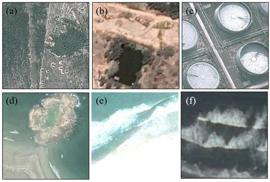
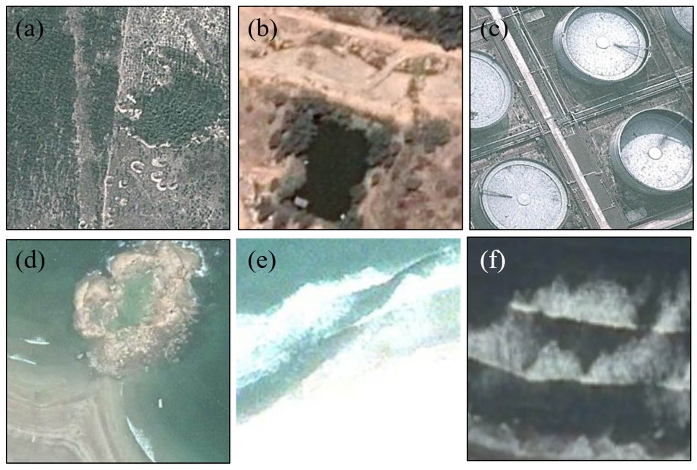
It is important to note that images partitioned from far-view satellite imagery represent a wide range of non-beach scenes, including but not limited to forests, man-made structures, harbors, rocky shorelines, offshore islands, water bodies, and clouds. The inclusion of such features introduced additional complexity to the rip detection model, as the model needs not only to identify rip currents but also to distinguish beach areas from other types of scenes. Furthermore, the partitioned images can contain breaking wave scenes that exhibit visual contrast features similar to those of rip currents. Examples of visually misleading images that are prone to false detections are shown in Figure 4. To ensure sufficient representation of such “hard sample” features in the training dataset, we applied a hard sample mining procedure. A preliminary model was first trained and then used to process a new set of images. Images that produced false detections in this step were identified as hard samples and subsequently incorporated into the training dataset for training the final detector. In summary, the dataset prepared in this study extends beyond the datasets previously used in related research, offering a new set of images and annotations tailored for rip current detection using satellite imagery.

2.3. Model Training and Evaluation

The YOLO11s architecture and pretrained models were employed in the detection pipeline to build the rip detector and the beach classifier. The models were trained on a workstation with NVIDIA GeForce Ada2000 GPU and 64 GB of RAM. The deep learning framework employed was PyTorch version 2.5, Python version 3.12, and CUDA version 11.2. Both the detection and classification model were trained twice. The first round aimed to capture general, fundamental features common across the dataset (source 1 and 2), while the second fine-tuning round focused on learning more specific and challenging features associated with partitioned images of different sizes. The rip detector was first trained using a set of 3638 images of mostly unambiguous scenes, including 897 positive samples. Approximately 5% of the training images were used for validation. These images were selected as examples in which the presence or absence of a rip current could be distinguished clearly. The rip detector was subsequently fine-tuned by adding 480 hard images (including 291 positive samples) to the training dataset. These hard samples were identified through the hard sample mining procedure and included visually misleading positive and negative cases. For the beach classifier, first-round training used a set of 21,765 images, including 7088 beach scenes. Approximately 10% of these images were set aside for validation. The training set covered a wide range of scenes, including forests, man-made structures, harbors, rocky shorelines, offshore islands, water bodies, and clouds. The beach classifier was subsequently fine-tuned with a set of 12,625 images, of which 3923 depicted beach scenes. The second training set was constructed with an emphasis on distinguishing beach scenes with intense breaking waves from land features with pronounced edges. The key training hyperparameters of the YOLO11s models and the corresponding validation performance for the detector and classifier are summarized in

Table 3. Key hyperparameters and performance of YOLO11 detection (D) and classification (C) models.

	Parameter	Value
Hyperparameters	batch (batch size)	16
	imgsz (image size)	224
	optimizer	Adam
	lr0 (learning rate)	0.001
	box (weight of the box loss)	0.5 (D)
	cls (weight of the classification loss)	10 (D)
	dfl (weight of the distribution focal loss)	2.5 (D)
Performance	parameter (M)	9.4 (D), 6.7 (C)
	size (MB)	18.3 (D), 10.5 (C)
	mAPval50	0.824 (D)
	acctop1	0.988 (C)

. Note that the loss function of the detection model consists of three components (i.e., box loss, classification loss, and focal loss), and their weights were adjusted to optimize mAP^val50. The same batch size, image size, optimizer choice, and learning rate were used in training the two models.

To evaluate the performance of the proposed rip detection pipeline, precision and recall were calculated as follows:

$$\mathrm{Precision}={\displaystyle \frac{TP}{TP+FP}},$$

(1)

$$\mathrm{Recall}={\displaystyle \frac{TP}{TP+FN}},$$

(2)

True positives (TPs) correspond to correctly detected rip currents, false positives (FPs) correspond to falsely detected rips, and false negatives (FNs) represent missed rip current detections. An IoU threshold of 0.5 was used to determine a correct detection. Note that IoU here quantifies the overlap between a predicted bounding box and a ground-truth bounding box. For rip current detection, inclusive detection of all possible occurrences without missing objects is perceived to be more critical than having false detections. Thus, to balance precision and recall, with a focus on recall, the F2 score was calculated as follows:

$$\mathrm{F}2={\displaystyle \frac{5}{4/Precision+1/Recall}},$$

(3)

In addition, to evaluate the overall performance of the method in correctly identifying the presence or absence of rip occurrence in an image, the accuracy is calculated as follows:

$$\mathrm{Accuracy}={\displaystyle \frac{N_{correct}}{N_{total}}},$$

(4)

where N_correct is the number of images for which the presence or absence of a rip current is correctly determined, and N_total is the total number of images in the testing dataset.

2.4. Rip Current Characterization

To characterize rip current occurrences in georeferenced satellite imagery, the size of rip currents, their occurrence time, and the corresponding nearby wave conditions are obtained to represent the spatial–temporal characteristics and environmental factors associated with rip occurrences. In this study, rip current size was approximated as the meter length of its annotated bounding box’s longer side, which was calculated as P × r, where the product of the bounding box pixel length is represented by P and pixel resolution by r. Rip occurrence time was equivalent to the recorded dates when the satellite image was captured. Nearby wave conditions were approximated using the ERA5 reanalysis data, since no nearby wave buoy observation data were available. The ERA5 is the fifth-generation reanalysis product by the European Centre for Medium-Range Weather Forecasts (ECMWF) for the global atmosphere, land surface, and ocean waves [47]. Specifically, two ocean wave variables, mean wave direction (MWD) and significant wave height (SWH), provided at regular grids of 0.5 degrees, were obtained from the “ERA5 hourly data on single levels from 1940 to present” dataset to represent the offshore wave conditions for those beaches identified with rip occurrences.

3. Results

3.1. Performance of Rip Detection Pipeline

The rip detection pipeline achieved satisfactory performance with an overall accuracy of 98.4%, a recall of 0.890, a precision of 0.633, and an F2 score of 0.823 on the 387 testing dataset images from the ESRI World Imagery dataset (source 3). The high accuracy indicates that this method is capable of reliably determining the presence of rip currents in far-view satellite imagery. The high recall, with comparatively lower precision, implies that the method tends to prioritize detecting all possible rip currents within an image, which comes with the trade-off of false detections. This tendency is desired for locating small objects in a large field of view, as minimizing missing objects is more critical than having false detections.

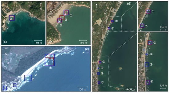
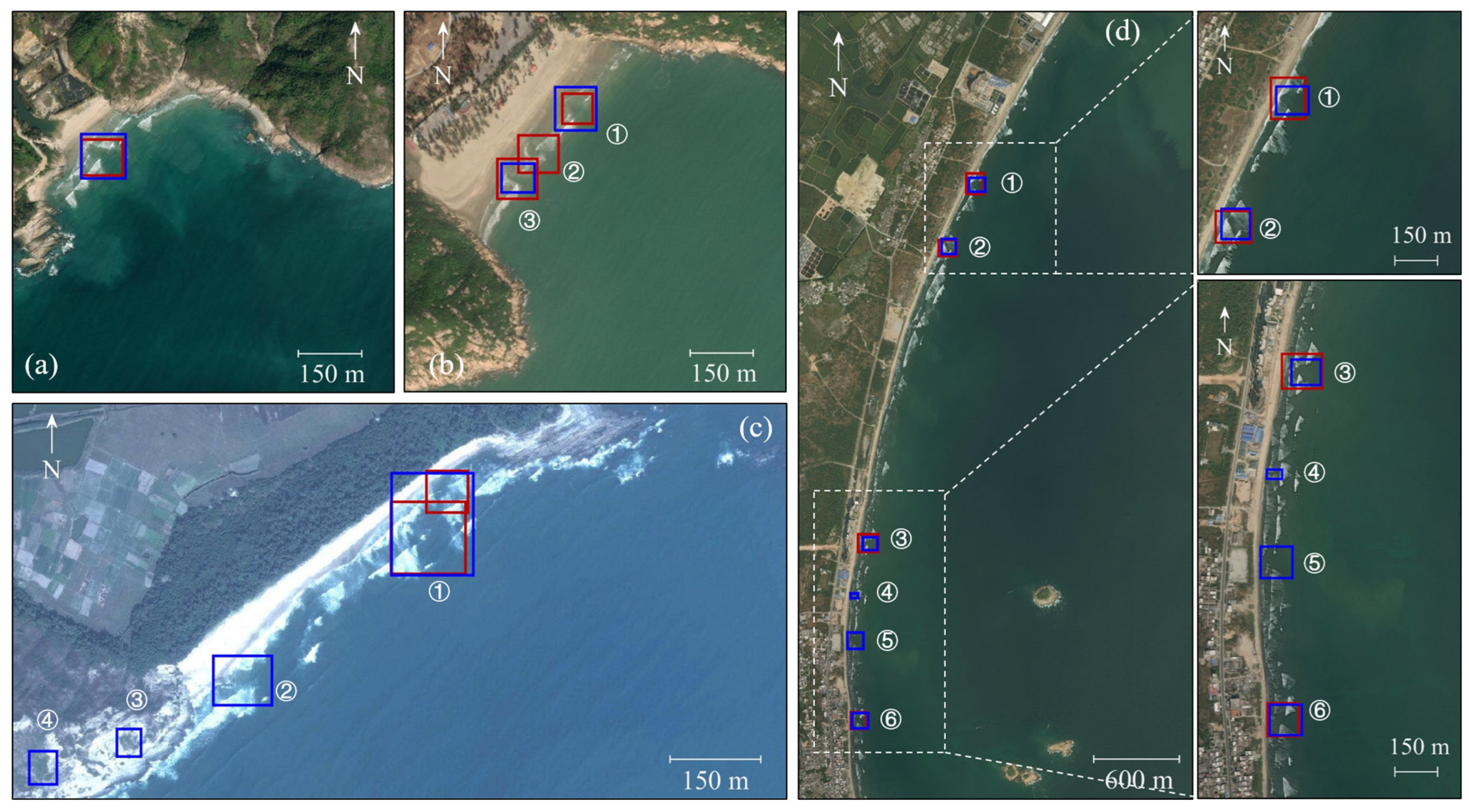
To further illustrate the method’s performance in detecting rip currents as small objects within far-view satellite imagery, examples for different shoreline stretches ranging from hundreds to thousands of meters are presented in Figure 5, in which the red rectangle boxes represent the annotated rip currents and the blue boxes represent the predicted bounding boxes. Figure 5a shows a relatively easy example in which a pronounced “V-shaped” rip current appearing in a dark, elongated region between bright breaking waves was correctly detected (i.e., TP). Figure 5b shows an example with a missed detection (i.e., FN) for a “curved” rip current ($②$ in Figure 5b), while two “jet” rips ($①$ and $③$ in Figure 5b) were correctly detected. This missed rip was initially identified as a candidate region but was later discarded because its corresponding augmented images did not provide sufficient detections for confirmation. The same situation applied to all other missed rip currents in the testing dataset. Despite this, the use of augmented images remains important for reducing spurious detections, which will be discussed in detail in Section 3.2. Figure 5c shows an example containing one correctly detected “jet” rip ($①$ in Figure 5c), along with three incorrect detections (i.e., FP), with dark vegetation zones in a light-colored background land ($③$ and $④$ in Figure 5c) and non-breaking calm water between bright breaking zones (② in Figure 5c) misidentified as rip currents. Among all false detections in the testing dataset, 18% (8 out of 45) were attributed to a land feature with pronounced color contrasts and rip-like edges, while 82% (37 out of 45) were associated with ambiguous patterns of wave breaking that can be more challenging to distinguish from wave breaking-induced rip currents. This challenging situation is also shown in Figure 5d, presenting an example of detections within a large field of view. Three “V-shaped” rips ($①$, $③$, and $⑥$ in Figure 5d) and one “mixed” type ($②$ in Figure 5d) were correctly detected along with two false detections ($④$ and $⑤$ in Figure 5d). As shown in the zoomed windows, the two false detections are attributed to the breaking wave patterns which exhibit a similar color contrasting feature as rip currents. In general, the detection pipeline can effectively capture small rip current objects within far-view satellite imagery, and the remaining false detections were mainly associated with an intense wave breaking-induced visual signature similar to that of a rip current.

In addition, to examine performance across different imagery sources, an additional evaluation was conducted using 125 far-view images from the Google Earth Historical Imagery dataset (source 2). Note that source 2 is not a fully independent test set because it supplied close-view images for training the rip detector, though the far-view images used here were not directly used for training. Testing on the far-view images from source 2 yielded an accuracy of 94.4%, a recall of 0.864, a precision of 0.740, and an F2 score of 0.836. The slightly higher precision and F2 score, relative to source 3, are possibly attributable to source 2’s involvement in training. Meanwhile, the lower recall and accuracy may relate to the higher rip occurrence frequency in these 125 images, ~3.2 rips/image compared to ~0.13 rip/image in the 387 testing images of source 3. In general, the additional evaluation demonstrated the consistent performance of the detection pipeline across different data sources.

Overall, the proposed detection pipeline is capable of accurately identifying the presence or absence of rip currents in a far-view satellite image and detecting the locations of rip currents within the image most of time. Furthermore, considering that the testing image dataset was constructed from a source independent from those used in training, the pipeline’s performance also indicates the great potential of its applications to new locations.

3.2. Key Procedures to Remove Spurious Detections

Spurious detections were observed when applying rip detection to images partitioned from far-view satellite imagery, as rip current features may appear indistinct within visually complex scenes. To address this challenge, the proposed pipeline incorporates three specific procedures: (i) filtering out non-beach scenes using a beach classification model, (ii) performing rip detection on augmented images, and (iii) introducing a hard sample mining procedure when constructing the training dataset. The contributions of these procedures were examined by comparing precision, recall, F2 score, and accuracy under different combinations, as summarized in

Table 4. Performance comparison of combinations of three key procedures in detection pipeline.

Case	Key Procedures			Performance
	Non-Beach Scene Filtering	Rip Detection on Augmented Images	Hard Sample Mining	Precision	Recall	F2 Score	Accuracy
1	yes	yes	yes	0.632	0.890	0.823	0.984
2		yes	yes	0.302	0.934	0.659	0.849
3	yes		yes	0.337	0.945	0.695	0.963
4	yes	yes		0.405	0.747	0.639	0.966
5			yes	0.120	1.000	0.404	0.675
6		yes		0.102	0.791	0.336	0.619
7	yes			0.221	0.868	0.547	0.892
8				0.039	0.934	0.169	0.362

. Case 1, with all three procedures included, corresponds to the complete detection pipeline described in Section 3.1. The effects of each procedure are examined separately as follows.

First, the effect of non-beach scene filtering, examined by comparing Case 1 and 2, suggests that this procedure is effective in reducing spurious detections in non-beach scenes. A notable increase in precision is observed when this procedure is applied, accompanied by improvements in the F2 score and overall accuracy, although a slight decrease in recall is also present. A similar pattern is seen in cases where the other two procedures were not used (i.e., Case 3 and 5, 4 and 6, 7 and 8). In addition, when non-beach scene filtering was included, the detection accuracy consistently remained above roughly 90% (i.e., Case 1, 3, 4, and 7), regardless of whether the other procedures were applied. This implies that filtering out non-beach scenes can help improve the reliability of determining whether rip currents are present, primarily by reducing false detections in rip-absent images.

Second, the effect of rip detection on augmented images, examined by comparing Case 1 and 3 (and similarly 2 and 5, 4 and 7, 6 and 8), indicates noticeable improvements in precision, F2 score, and accuracy, accompanied by a slight reduction in recall. The overall trend is similar to that observed when filtering out non-beach regions, though the magnitude of improvement is smaller. To further understand this difference, we compared the false detections in Case 2 and 3. In Case 2, 71% (138 out of 194) of the falsely detected rips corresponded to land features. In contrast, in Case 3, 88% (144 out of 164) of the false detections were related to visually ambiguous wave breaking patterns. This comparison suggests that performing rip detection on augmented images is particularly effective in reducing wave breaking-related false detections, while it has relatively limited ability to remove misleading non-beach features. Building on this observation, the higher precision achieved with non-beach scene filtering (Case 3) relative to rip detection on augmented images (Case 2) can be partially explained by the distribution of detected candidate regions, which were mostly non-beach scenes (i.e., 62% in Case 1–3 and 5 with hard sample mining, and 82% in Case 4 and 6–8 without hard sample mining). In short, rip detection on augmented images is not a substitute to non-beach scene filtering and vice versa, each addressing different sources of spurious detections in the overall pipeline.

Third, the effect of hard sample mining, examined by comparing Case 1 and 4 (and similarly 2 and 6, 3 and 7, 5 and 8), indicates noticeable improvements in both precision and recall, accompanied by high F2 scores and accuracy. This outcome, achieved without sacrificing recall, highlights the importance of including appropriately challenging samples in the training dataset for enhancing overall detection performance. Nevertheless, when hard sample mining was applied alone (Case 5), the low precision and F2 score suggest that the trained detection model struggled to distinguish rip currents from spurious regions. This limitation is likely due to the model’s restricted generalization when applied to testing images that differ substantially from the training set. When combined with non-beach scene filtering and rip detection on augmented images (Case 1), the substantial improvement in precision demonstrates the effectiveness of these complementary procedures in removing spurious non-rip regions, thereby enhancing the method’s generalization to new datasets.

Overall, all cases consistently exhibit higher recall than precision, indicating that the detection pipeline prioritizes capturing true rip currents, even at the cost of some false detections. Across the different cases, variations in F2 score and accuracy follow the same trend as precision, further emphasizing that addressing spurious detections is crucial for improving overall detection performance. Each of the three key procedures contributed notably to improving precision and accuracy, and the combination of all three produced the best results on the testing dataset, demonstrating potential for general application at new locations.

3.3. Rip Current Occurrence and Characterization

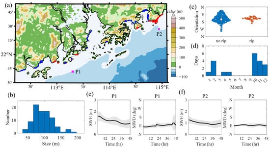
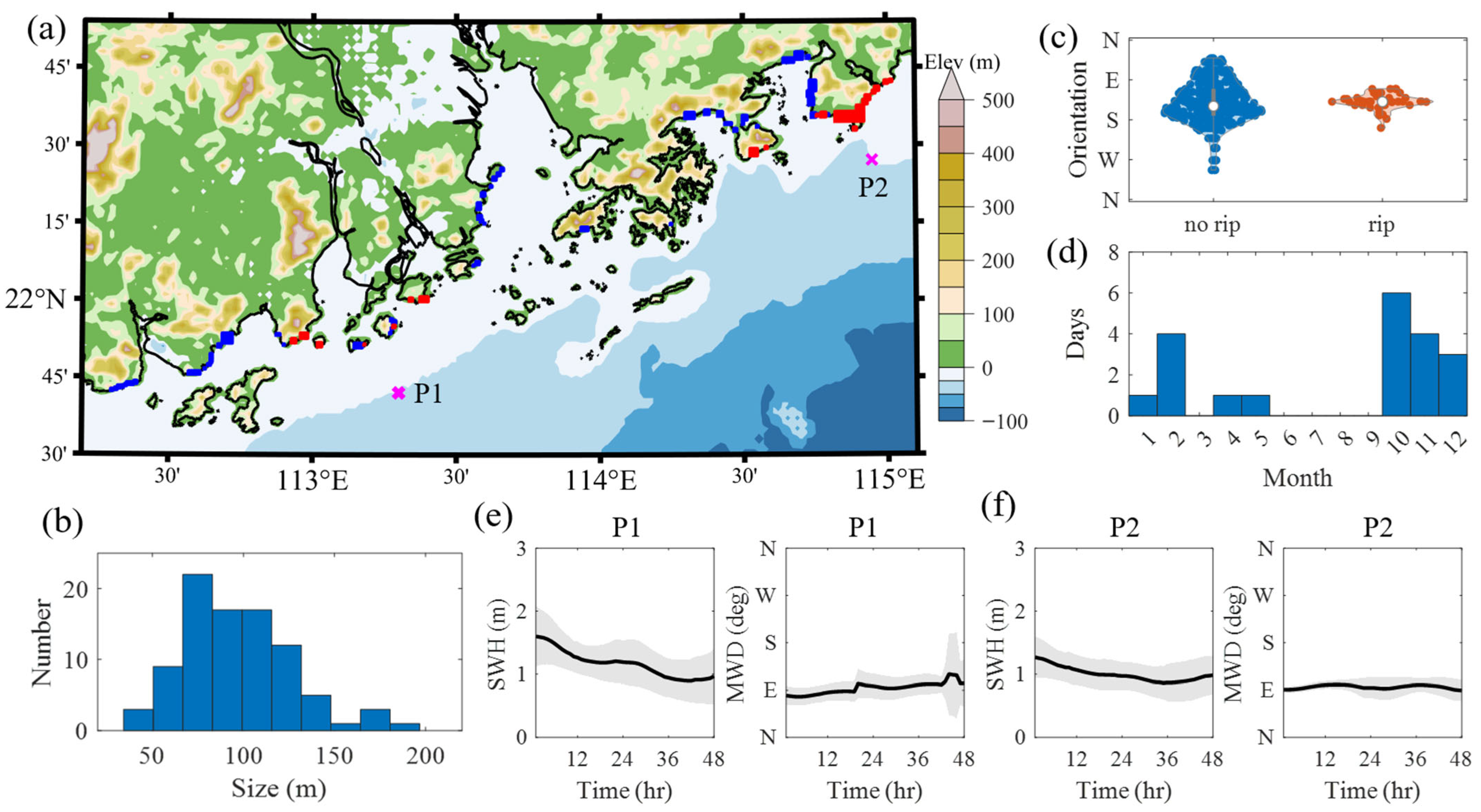
Rip currents detected from georeferenced satellite imagery can provide valuable spatial information for characterizing their occurrences. To demonstrate this, rip current occurrences in the Guangdong–Hong Kong–Macao Greater Bay Area (GBA) were characterized based on the georeferenced images in the ESRI World Imagery dataset captured during 2008 and 2021. Rip currents were identified in 18 out of a total of 71 beaches. As shown in Figure 6b, the majority of identified rips were between 50 and 150 m, which is consistent with the spatial scale of previously observed rip currents [3,20]. The beaches with observed rip current occurrences (red marks in Figure 6a) appear to be concentrated in two regions (approximately 113–113.5°E and 114.5–115°E) that are more directly exposed to the open ocean. In contrast, beaches without rip occurrence (blue marks in Figure 6a) are mainly located inside bays or in areas sheltered by archipelagos. It is possible that sheltering and obstruction effects reduce the wave energy reaching the nearshore zone, thereby limiting the wave forcing required for rip current generation.

To further elucidate the conditions for the observed rip occurrences at these beaches, shore-normal directions (Figure 6c), the monthly distribution of rip occurrences (Figure 6d), and wave conditions during rip occurrences (Figure 6e,f) were examined. Note that shore-normal direction refers to the direction perpendicular to the shoreline, pointing seaward. Comparing the distributions of shore-normal directions for beaches without and with rips (Figure 6c), we observed that rip occurrences tended to cluster at beaches facing approximately from E to S. On one hand, due to the general NE-SW shoreline orientation of the GBA, beaches facing E to S are more likely to align with the areas that are directly exposed to the ocean. On the other hand, the wave climate for this region is primarily dominated by strong northeasterly winter monsoons [48] which can generate stronger waves that are favorable for rip generation at E-facing beaches. This behavior is also reflected through the monthly distribution of rip occurrences (Figure 6d), which shows that rip currents mainly occurred from Oct to Feb, aligning with the winter monsoon season. Furthermore, the wave conditions associated with rip occurrences are examined in Figure 6e–f. Across the 92 dates for which satellite images were available, rip currents were identified on 20 dates. For these dates, the 48 h time series of offshore significant wave height (SWH) and mean wave direction (MWD) on the day of and the day preceding each rip occurrence were extracted from the ERA5 reanalysis and interpolated at the two grid points (P1 and P2) shown in Figure 6a. The detailed offshore wave conditions corresponding to each rip occurrence are summarized in

Table A3. A list of rip occurrence dates and the corresponding 48 h averaged significant wave height (SWH) and mean wave direction (MWD) at nearby ERA5 grid points (P1 or P2 in Figure 6) for the rip beaches detected from the satellite imagery in the Guangdong–Hong Kong–Macao Greater Bay Area.

	Rip Date	SWH (m)	MWD (°)	Location	Rip Beaches
1	2008-05-15	1.32	101	P2	DongHeCun, DongShanHai,
2	2010-10-23	1.01	122	P1	HeiShaWanBeach
3	2010-11-25	0.97	86	P2	HuangBuZhen, HuiDongXian, HuiDongXian_East, YijingWan
4	2013-10-24	0.67	76	P2	DongHeCun, DongShanHai, GangKouZhen, GaoYangWei, HuangBuZhen, PingHai
5	2013-10-29	0.96	96	P2	HuiDongXian_East
6	2017-02-16	1.16	108	P2	HuiDongXian, HuiDongXian_East, YijingWan
7	2017-11-01	1.29	85	P1	FeiShaWan
8	2018-10-30	1.28	92	P2	XiYongBeach
9	2019-11-11	1.09	124	P2	ChangShaTou
10	2019-11-24	0.71	84	P1	FeiShaWan
11	2019-12-14	1.02	94	P2	HK-DaLangWan
12	2021-01-26	0.90	101	P2	DongHeCun, DongShanHai, GaoYangWei, HuangBuZhen, YijingWan
13	2021-02-14	0.66	97	P2	HuiDongXian, HuiDongXian_East
14	2021-10-06	1.60	89	P1	FeiShaWan
15	2021-12-05	1.40	78	P1	JinShaWan
16	2022-04-06	0.95	99	P1	CaoTangWan
17	2022-10-14	1.37	81	P1	ChongKouWan, JinShaWan
18	2022-12-09	0.85	74	P2	HuiDongXian, HuiDongXian_East
19	2023-02-23	1.21	93	P2	DongHeCun, DongShanHai, GangKouZhen
20	2023-02-28	1.33	93	P1	HeiShaWanBeach

. The mean values of the 48 h time series and their variations, expressed as one standard deviation, are shown in Figure 6e,f. Moderate wave energy, with wave heights of approximately 1–2 m, was observed for both regions. More notable is the consistently easterly wave direction, which aligns with the previously described northeasterly monsoon-generated wave conditions. To summarize, the observed rip occurrences suggest that in the GBA, rip currents tended to develop at east- to southeast-facing open beaches during the winter monsoon period, when onshore-directed waves may create conditions favorable for rip formation. It should be noted that, given the limited number of positive rip current samples in this georeferenced image dataset, the above analysis reflects only one possible set of conditions associated with rip occurrences in this region. Nevertheless, this analysis illustrates the potential usage of rip detection from georeferenced satellite imagery for rip current characterization and hazard assessment studies. Future work can be effectively supported by applying the proposed detection framework to an extended set of satellite imagery.

4. Discussion

4.1. Comparative Experiments

This study presents a pipeline for detecting small rip current objects within high-resolution satellite imagery. It is important to note that the proposed pipeline is not intended to replace existing rip current detection models. Instead, existing models that focus on detecting rip currents in close-view optical images serve as the detector component within the proposed pipeline. Under this context, comparative experiments were conducted by replacing the YOLO11 detector in the pipeline with YOLOv5 and YOLOv8, two models that have been frequently used in rip current detection studies [34,37]. The two alternative detectors were trained from YOLOv5s and YOLOv8s pretrained models using the same training images and annotations as YOLO11. For consistency, hard sample mining was not applied because the mined samples depend on the detector used, and excluding them ensures that all three detectors were trained on an identical dataset. For baseline comparison, detector-level performance was first evaluated using a set of close-view testing imagery containing 511 beach images (including 117 positive samples) that were randomly selected from source 2 and source 3 with no overlap with the training data. For overall performance comparison, the pipeline’s performance (without hard sample mining, i.e., Case 4 in Table 4) was then compared across different detectors using the 387 far-view testing images from source 3.

The results of the comparative experiments are shown in

Table 5. Performance comparison among different rip detectors within detection pipeline.

Testing Scenario	Detector Model	Precision	Recall	F2 Score	Accuracy
Close-view images	YOLO11	0.895	0.803	0.820	0.933
	YOLOv8	0.883	0.838	0.846	0.937
	YOLOv5	0.854	0.752	0.771	0.914
Far-view images (Case 4)	YOLO11	0.405	0.747	0.639	0.966
	YOLOv8	0.371	0.538	0.494	0.931
	YOLOv5	0.414	0.582	0.584	0.941
Far-view images (Case 7)	YOLO11	0.221	0.868	0.547	0.892
	YOLOv8	0.202	0.835	0.513	0.865
	YOLOv5	0.200	0.813	0.505	0.889

. At the detector-level, YOLO11 and YOLOv8 performed similarly and both slightly outperformed YOLOv5 across all four metrics on close-view images. This indicates that the YOLO11 model selected for this study is comparable to established detectors for the rip detection task. At the pipeline level, the version incorporating YOLO11 achieved higher overall performance on far-view images compared to those incorporating YOLOv8 or YOLOv5. The most notable differences were the lower recalls and consequently lower F2 scores associated with YOLOv8 and YOLOv5. To further examine this result, we reviewed the testing scenario without augmented image detection (i.e., Case 7 in Table 4), and similar performance was observed across the three detectors. Since image augmentation was intended to represent rips at different relative sizes in input images, the better performance of YOLO11 may be attributed to the spatial attention module (C2PSA), which may lead to more accurate detection at varying scales by enhancing its ability to detect small or partially occluded objects [46]. In short, these findings indicate that the selected YOLO11 model possesses a capacity similar to established detectors on close-view imagery, while its use within the proposed pipeline appears to yield comparatively higher overall performance.

The comparative experiment results also indicate that the performance of the proposed pipeline may vary depending on the rip detector employed. In this study, the three detectors compared were based on different versions of the YOLO architecture, while various other two-stage and one-stage detection models (e.g., Faster R-CNN, MobileNet, EfficientNet) could in principle be employed within this pipeline. These alternatives were not further examined here, considering that the primary focus of the present work is on pipeline design rather than on comprehensive benchmarking of detector architectures. Future work that incorporates a broader range of detection models into this pipeline and conducts systematic comparisons may provide additional insight for further improving overall rip detection in far-view satellite imagery.

4.2. Small Object Detection Challenges, Limitations, and Future Directions

The challenge of detecting small rip current objects within satellite imagery is discussed. In a practical setting, where no prior knowledge of rip locations is available, detecting rip occurrence requires searching for small rip features within a large field of view. Directly inputting a high-resolution far-view image into a detector is impractical because the image size exceeds the limits of typical detection models. This would either require an excessively large and computationally expensive model or significant image downscaling, which could obscure small yet critical features of rip currents. To address this, the proposed detection pipeline first partitions a large far-view image into multiple small close-view images. Rip detection is then conducted on these partitioned close-view images, an approach that has been shown to be feasible in previous rip detection studies. A critical step of the pipeline is combining the detection results from the small images to determine the final positions of rip currents within the original far-view image, as partitioned images often contain a wide range of scenes with misleading visual features similar to those of rip currents. To reduce spurious detections, the pipeline incorporates three key procedures: non-beach scene filtering with a beach classifier, rip detection on augmented images, and hard sample mining. The effectiveness of this design was validated on an independent testing dataset, demonstrating that the method can accurately identify the presence or absence of rip currents in a far-view satellite image and locate the rip currents within the image in most cases.

Nevertheless, it was also observed that the detection performance was mainly affected by false detections related to breaking wave patterns with similar color and morphological features as rip currents. This suggests that additional spatial and contextual cues, such as shoreline orientation, surf zone extent, and cross-shore distance, may be incorporated to improve discrimination. Future work could explore integrating such environmental and geometric information, either through feature engineering or by designing model components that explicitly account for spatial relationships in the nearshore environment.

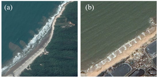
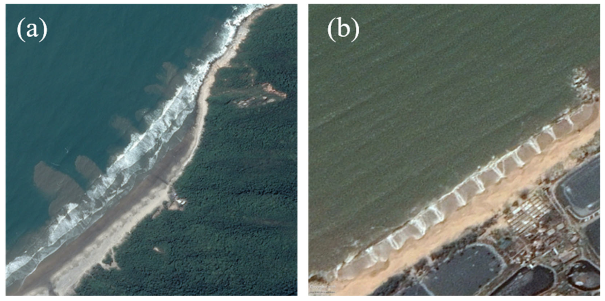
Only rip currents that appear as dark regions between breaking waves were detected, while those appearing as sediment plumes (Figure 7a) or swash rips (Figure 7b) were not considered in this study. Although these two rip types were observed in satellite images (source 2 and 3), they were excluded because their limited numbers were insufficient for training. These rips are possibly hydrodynamically controlled and may form under different conditions from those appearing in the darker gap between breaking waves. This also points to a future direction of applying the proposed method to other rip current types, which may support a more comprehensive assessment of rip occurrences at a beach.

Detecting rip currents is different from many other object detection tasks, as the identification of rips relies heavily on visual interpretation of rip-induced water surface features. Given the limited availability of concurrent in situ velocity measurements, interpretation based on established descriptions and observational experiences remains the most practical approach. Within this context, developing a large and standardized image dataset of rip currents would be valuable for advancing scientific understanding of this coastal process. Using satellite imagery with a large field of view, the proposed method can facilitate the compilation of such a dataset and support future analyses of rip currents.

4.3. Computational Efficiency and Scalability

Different from existing studies that target real-time detection of rip currents [34,38], which is critical for immediate maritime safety applications, the proposed framework is not intended for real-time monitoring. This reflects not only the inference time associated with the partition–merge detection strategy, but also the intrinsic sampling nature of satellite imagery which is acquired at discrete revisit intervals rather than continuously. Considering the large spatial coverage and the availability of georeferenced information, the proposed pipeline is more suitable for offline or periodic applications where near-instantaneous detection is not required, such as mapping rip-prone beaches, seasonal rip hazard assessment, and post-storm surveys. These analyses are usually integrated into broader research or planning cycles where rapid decision-making is not the goal. Under such context, processing time on the order of hours to one day per application scenario is operationally acceptable. Accordingly, the fundamental design principle of the proposed pipeline prioritizes accuracy and robustness over real-time speed, trading a single global detection for multiple localized detections on partitioned images while enabling the processing of high-resolution far-view satellite imagery without excessive downscaling and remaining computationally feasible.

Although second- to minute-timescale delivery is not required for the targeted applications, timeliness remains a key operational consideration. The processing time for experiments of this study, conducted on a workstation equipped with NVIDIA GeForce Ada2000 GPU and Intel Core i7-13700HX 16-core (8P + 8E) CPU, is reported. For a typical far-view satellite image (approximately 2500 × 2500 pixels), the processing time was on the order of 1 min. Inference time ranged from a few seconds (e.g., approximately 10 s for a 1088 × 1088 pixel image) to up to 22 min for the largest image (15,783 × 7564 pixels) used in this study. For a realistic large-scale analysis scenario, such as the Guangdong–Hong Kong–Macao Greater Bay Area (GBA) case study, the total processing time for the 378 far-view georeferenced images was 10 h and 25 min. A breakdown indicates that approximately 2 h and 13 min was spent on image partitioning, 8 h and 7 min on rip detection over partitioned images, approximately 1 min on result merging, approximately 1 min on non-beach scene filtering, approximately 2 min on rip detection over augmented images, and approximately 1 min on final detection. The result indicates that the first two steps in the detection workflow are the most time-consuming components of the pipeline.

Notably, both steps are inherently parallelizable. Preliminary optimization experiments using 66 far-view GBA images showed that parallel processing with eight cores reduced partitioning time to approximately 20% of the sequential (eight-core) time. For rip detection over partitioned images, batch inference with batch sizes of 8, 16, and 32 reduced inference time to approximately 75%, 47%, and 37% of the sequential (batch size 1) configuration, respectively. Assuming similar efficiency across the full dataset, the total processing time for the 378 images could potentially be reduced from 10.5 h to approximately 3.5 h under parallel settings. Additional optimization strategies, such as incorporating spatial and contextual cues for early filtering to reduce the number of partitioned images requiring inference, may further improve performance.

In terms of scalability, the dominant factor in processing time is the number of partitioned images from the input georeferenced image. Because the partition window size is defined in physical units (meters), the number of partitioned images is fundamentally determined by the actual spatial extent of the scene. Considering that shorelines are commonly obliquely oriented relative to the image axes, the mapped area scales approximately with the square of the shoreline stretch. Consequently, both the number of partitioned images and processing time increase in proportion to the square of shoreline stretch for a given resolution. The 4 GB size limit of the georeferenced image format (i.e., GeoTIFF) provides a practical upper bound for a single-scene input, which corresponds to an approximately 37,000 × 37,000 pixel RGB image (approximately 30 km shoreline stretch at 0.6 m/pixel). It is estimated that processing such a scene would require approximately 5.6 h (1.8 h with aforementioned optimization) under the same hardware condition. Therefore, within this image size bound, the proposed pipeline remains operational for its intended offline applications.

While the current framework is designed for offline usage, it may be extended toward near-real-time applications under conditions of higher temporal sampling, relatively small spatial extent, and optimized inference efficiency. For example, airborne imagery collected by UAVs or crewed aircraft provides georeferenced optical data with more flexible acquisition timing. In such cases, imagery could be collected during high-risk conditions and processed shortly after acquisition to support timely assessment of hazardous rip current conditions.

5. Conclusions

This study presents a pipeline for detecting small rip current objects within high-resolution satellite imagery. Different from previous work that focused on identifying rips in close-view beach images, this method has addressed the challenge of locating a rip current as a small object within a large-field-of-view satellite image covering various beach and non-beach scenes. The basic workflow of the developed pipeline consists of partitioning a large satellite image into small regions, performing rip current detection on each partitioned small image, and combining the detection results to determine the final rip position within the original large image. In this process, directly merging detection results from partitioned images can lead to a notable number of false detections, because the partitioned images contain a wide range of scenes including many that exhibit misleading visual features similar to those of rip currents. To reduce spurious detections, we specially designed additional procedures to be executed after merging. A beach classification model was applied to filter out non-beach scenes, followed by application of the rip detection model on a set of images augmented from detected candidate regions to double-check the results. By including these procedures, we have shown that the rip detection pipeline is capable of reliably determining rip presence in far-view satellite imagery and locating most rip currents, with an overall accuracy of 98.4%, a recall of 0.890, a precision of 0.633, and an F2 score of 0.823 achieved on the testing set. As the testing images are from a different data source compared to those used in training, this result also indicates the pipeline’s great potential for future applications to new locations.

A new rip current image dataset containing far-view satellite imagery was developed in this study. While existing rip current image datasets have primarily focused on close-view beach scenes, where rips appear as large and distinct targets, the new dataset features far-view images sourced from Google Earth Historical Imagery and the ESRI World Imagery dataset, representing broader shoreline stretches. These images were further partitioned into small regions to construct a training dataset that captures a wide range of coastal scenarios, including easy samples of beach scenes with and without rip, unambiguous non-beach regions such as forests, man-made structures, harbors, rocky shorelines, offshore islands, water bodies, clouds, and challenging cases where breaking waves or land features exhibit color contrasts resembling rip current signatures. With the new dataset, we demonstrated the potential usage of rip current detection with satellite imagery in rip current characterization for the Guangdong–Hong Kong–Macao Greater Bay Area (GBA). The results show that rip currents tended to occur at east- to southeast-facing open beaches during the winter monsoon period, when moderate-energy, onshore-directed waves may create conditions favorable for rip formation. The case study also demonstrates that the proposed pipeline, unlike existing near-real-time rip current monitoring systems, provides an effective high-accuracy analysis tool for offline or periodic applications using satellite imagery. Overall, the development of this dataset represents a meaningful step toward expanding available resources for rip current research and improving automated detection in complex coastal environments.

References

- Brander, R.W.; Bradstreet, A.; Sherker, S.; MacMahan, J. Responses of Swimmers Caught in Rip Currents: Perspectives on Mitigating the Global Rip Current Hazard. Int. J. Aquat. Res. Educ. 2011, 5, 11. [Google Scholar] [CrossRef] [Scilit]
- Drozdzewski, D.; Shaw, W.; Dominey-Howes, D.; Brander, R.; Walton, T.; Gero, A.; Sherker, S.; Goff, J.; Edwick, B. Surveying Rip Current Survivors: Preliminary Insights into the Experiences of Being Caught in Rip Currents. Nat. Hazards Earth Syst. Sci. 2012, 12, 1201–1211. [Google Scholar] [CrossRef] [Scilit]
- Castelle, B.; Scott, T.; Brander, R.W.; McCarroll, R.J. Rip Current Types, Circulation and Hazard. Earth-Sci. Rev. 2016, 163, 1–21. [Google Scholar] [CrossRef] [Scilit]
- MacMahan, J.H.; Thornton, E.B.; Reniers, A.J.H.M. Rip Current Review. Coast. Eng. 2006, 53, 191–208. [Google Scholar] [CrossRef] [Scilit]
- McCarroll, R.J.; Castelle, B.; Brander, R.W.; Scott, T. Modelling Rip Current Flow and Bather Escape Strategies across a Transverse Bar and Rip Channel Morphology. Geomorphology 2015, 246, 502–518. [Google Scholar] [CrossRef] [Scilit]
- Moulton, M.; Elgar, S.; Raubenheimer, B.; Warner, J.C.; Kumar, N. Rip Currents and Alongshore Flows in Single Channels Dredged in the Surf Zone. J. Geophys. Res. Ocean. 2017, 122, 3799–3816. [Google Scholar] [CrossRef] [Scilit]
- Schönhofer, J.; Dudkowska, A. Rip Currents in the Southern Baltic Sea Multi-Bar Nearshore Zone. Cont. Shelf Res. 2021, 212, 104324. [Google Scholar] [CrossRef] [Scilit]
- Pattiaratchi, C.; Olsson, D.; Hetzel, Y.; Lowe, R. Wave-Driven Circulation Patterns in the Lee of Groynes. Cont. Shelf Res. 2009, 29, 1961–1974. [Google Scholar] [CrossRef] [Scilit]
- Scott, T.; Austin, M.; Masselink, G.; Russell, P. Dynamics of Rip Currents Associated with Groynes—Field Measurements, Modelling and Implications for Beach Safety. Coast. Eng. 2016, 107, 53–69. [Google Scholar] [CrossRef] [Scilit]
- Castelle, B.; Coco, G. Surf Zone Flushing on Embayed Beaches. Geophys. Res. Lett. 2013, 40, 2206–2210. [Google Scholar] [CrossRef] [Scilit]
- Mouragues, A.; Martins, K.; Bonneton, P.; Castelle, B. Headland Rip Very Low Frequency Fluctuations and Surfzone Eddies During High-Energy Wave Events. J. Phys. Oceanogr. 2022, 52, 2935–2956. [Google Scholar] [CrossRef] [Scilit]
- Spydell, M.; Feddersen, F. Lagrangian Drifter Dispersion in the Surf Zone: Directionally Spread, Normally Incident Waves. J. Phys. Oceanogr. 2009, 39, 809–830. [Google Scholar] [CrossRef] [Scilit]
- Clark, D.B.; Elgar, S.; Raubenheimer, B. Vorticity Generation by Short-Crested Wave Breaking. Geophys. Res. Lett. 2012, 39, 24604. [Google Scholar] [CrossRef] [Scilit]
- Elgar, S.; Raubenheimer, B. Field Evidence of Inverse Energy Cascades in the Surfzone. J. Phys. Oceanogr. 2020, 50, 2315–2321. [Google Scholar] [CrossRef] [Scilit]
- Macmahan, J.; Thornton, E.; Stanton, T.; Reniers, A. RIPEX: Observations of a Rip Current System. Mar. Geol. 2005, 218, 113–134. [Google Scholar] [CrossRef] [Scilit]
- Spydell, M.; Feddersen, F.; Guza, R.T.; Schmidt, W.E. Observing Surf-Zone Dispersion with Drifters. J. Phys. Oceanogr. 2007, 37, 2920–2939. [Google Scholar] [CrossRef] [Scilit]
- McCarroll, R.J.; Brander, R.W.; Turner, I.L.; Power, H.E.; Mortlock, T.R. Lagrangian Observations of Circulation on an Embayed Beach with Headland Rip Currents. Mar. Geol. 2014, 355, 173–188. [Google Scholar] [CrossRef] [Scilit]
- Leatherman, S.B.; Leatherman, S.P. Techniques for Detecting and Measuring Rip Currents. Int. J. Earth Sci. Geophys. 2017, 3, 1–2. [Google Scholar] [CrossRef] [Scilit] [PubMed]
- Shepard, F.P.; Emery, K.O.; La Fond, E.C. Rip Currents: A Process of Geological Importance. J. Geol. 1941, 49, 337–369. [Google Scholar] [CrossRef] [Scilit]
- Dalrymple, R.A.; MacMahan, J.H.; Reniers, A.J.; Nelko, V. Rip Currents. Annu. Rev. Fluid Mech. 2011, 43, 551–581. [Google Scholar] [CrossRef] [Scilit]
- Holman, R.A.; Symonds, G.; Thornton, E.B.; Ranasinghe, R. Rip Spacing and Persistence on an Embayed Beach. J. Geophys. Res. 2006, 111, 2005JC002965. [Google Scholar] [CrossRef] [Scilit]
- Murray, T.; Cartwright, N.; Tomlinson, R. Video-Imaging of Transient Rip Currents on the Gold Coast Open Beaches. J. Coast. Res. 2013, 165, 1809–1814. [Google Scholar] [CrossRef] [Scilit]
- Floc’h, F.; Mabiala, G.R.; Almar, R.; Castelle, B.; Hall, N.; Du Penhoat, Y.; Scott, T.; Delacourt, C. Flash Rip Statistics from Video Images. J. Coast. Res. 2018, 81, 100–106. [Google Scholar] [CrossRef] [Scilit]
- Liu, Y.; Wu, C.H. Lifeguarding Operational Camera Kiosk System (LOCKS) for Flash Rip Warning: Development and Application. Coast. Eng. 2019, 152, 103537. [Google Scholar] [CrossRef] [Scilit]
- Chickadel, C.C.; Holman, R.A.; Freilich, M.H. An Optical Technique for the Measurement of Longshore Currents. J. Geophys. Res. 2003, 108, 2003JC001774. [Google Scholar] [CrossRef] [Scilit]
- Philip, S.; Pang, A. Detecting and Visualizing Rip Current Using Optical Flow. In Proceedings of the EuroVis 2016—Short Papers, Groningen, The Netherlands, 6–10 June 2016. [Google Scholar]
- Anderson, D.; Bak, A.S.; Brodie, K.L.; Cohn, N.; Holman, R.A.; Stanley, J. Quantifying Optically Derived Two-Dimensional Wave-Averaged Currents in the Surf Zone. Remote Sens. 2021, 13, 690. [Google Scholar] [CrossRef] [Scilit]
- McGill, S. Rip Current and Channel Detection Using Surfcams and Optical Flow. Shore Beach 2022, 90, 50–58. [Google Scholar] [CrossRef] [Scilit]
- De Silva, A.; Zhao, M.; Stewart, D.; Khan, F.H.; Dusek, G.; Davis, J.; Pang, A. RipViz: Finding Rip Currents by Learning Pathline Behavior. IEEE Trans. Vis. Comput. Graph. 2024, 30, 3930–3944. [Google Scholar] [CrossRef] [Scilit]
- Maryan, C.; Hoque, M.T.; Michael, C.; Ioup, E.; Abdelguerfi, M. Machine Learning Applications in Detecting Rip Channels from Images. Appl. Soft Comput. 2019, 78, 84–93. [Google Scholar] [CrossRef] [Scilit]
- De Silva, A.; Mori, I.; Dusek, G.; Davis, J.; Pang, A. Automated Rip Current Detection with Region Based Convolutional Neural Networks. Coast. Eng. 2021, 166, 103859. [Google Scholar] [CrossRef] [Scilit]
- Rampal, N.; Shand, T.; Wooler, A.; Rautenbach, C. Interpretable Deep Learning Applied to Rip Current Detection and Localization. Remote Sens. 2022, 14, 6048. [Google Scholar] [CrossRef] [Scilit]
- Dumitriu, A.; Tatui, F.; Miron, F.; Ionescu, R.T.; Timofte, R. Rip Current Segmentation: A Novel Benchmark and YOLOv8 Baseline Results. In Proceedings of the 2023 IEEE/CVF Conference on Computer Vision and Pattern Recognition Workshops (CVPRW), Vancouver, BC, Canada, 18–22 June 2023; pp. 1261–1271. [Google Scholar]
- Zhu, D.; Qi, R.; Hu, P.; Su, Q.; Qin, X.; Li, Z. YOLO-Rip: A Modified Lightweight Network for Rip Currents Detection. Front. Mar. Sci. 2022, 9, 930478. [Google Scholar] [CrossRef] [Scilit]
- Rashid, A.H.; Razzak, I.; Tanveer, M.; Hobbs, M. Reducing Rip Current Drowning: An Improved Residual Based Lightweight Deep Architecture for Rip Detection. ISA Trans. 2023, 132, 199–207. [Google Scholar] [CrossRef] [Scilit]
- Rashid, A.H.; Razzak, I.; Tanveer, M.; Robles-Kelly, A. RipDet: A Fast and Lightweight Deep Neural Network for Rip Currents Detection. In Proceedings of the 2021 International Joint Conference on Neural Networks (IJCNN), Shenzhen, China, 18 July 2021; pp. 1–6. [Google Scholar]
- Choi, J.; Rajendran, M.; Cheol Suh, Y. Explainable Rip Current Detection and Visualization with XAI EigenCAM. In Proceedings of the 2024 26th International Conference on Advanced Communications Technology (ICACT), Pyeong Chang, Republic of Korea, 4 February 2024; pp. 1–6. [Google Scholar]
- Khan, F.H.; Stewart, D.; De Silva, A.; Palinkas, A.; Dusek, G.; Davis, J.; Pang, A. RipScout: Realtime ML-Assisted Rip Current Detection and Automated Data Collection Using UAVs. IEEE J. Sel. Top. Appl. Earth Obs. Remote Sens. 2025, 18, 7742–7755. [Google Scholar] [CrossRef] [Scilit]
- Zhang, Y.; Huang, W.; Liu, X.; Zhang, C.; Xu, G.; Wang, B. Rip Current Hazard at Coastal Recreational Beaches in China. Ocean Coast. Manag. 2021, 210, 105734. [Google Scholar] [CrossRef] [Scilit]
- Hu, P.; Li, Z.; Zhu, D.; Su, Q.; Li, G. Types and Statistical Analysis of Rip Currents at 14 Beaches in the Guangdong Province. Haiyang Xuebao 2022, 44, 140–149. [Google Scholar]
- Mahat, N.F.; Saleh, E.; Azmi, N.F.; Sidik, M.J.; Al-Azad, S. The Potential of Rip Current Formation Using Google Earth Pro Platform—A Case Study at West Coast of Sabah, Malaysia. Environ. Ecol. Res. 2023, 11, 1039–1046. [Google Scholar] [CrossRef] [Scilit]
- Wei, W.; Cheng, Y.; He, J.; Zhu, X. A Review of Small Object Detection Based on Deep Learning. Neural Comput. Appl. 2024, 36, 6283–6303. [Google Scholar] [CrossRef] [Scilit]
- Nikouei, M.; Baroutian, B.; Nabavi, S.; Taraghi, F.; Aghaei, A.; Sajedi, A.; Moghaddam, M.E. Small Object Detection: A Comprehensive Survey on Challenges, Techniques and Real-World Applications. Intell. Syst. Appl. 2025, 27, 200561. [Google Scholar] [CrossRef] [Scilit]
- Wang, H.-M.; Doong, D.-J.; Lai, J.-W. Rip Current Identification in Optical Images Using Wavelet Transform. J. Mar. Sci. Eng. 2025, 13, 707. [Google Scholar] [CrossRef] [Scilit]
- Jocher, G.; Qiu, J. Ultralytics YOLO11. 2024. Available online: https://github.com/ultralytics/ultralytics (accessed on 18 January 2026).
- Khanam, R.; Hussain, M. YOLOv11: An Overview of the Key Architectural Enhancements. arXiv 2024, arXiv:2410.17725. [Google Scholar] [CrossRef] [Scilit]
- Hersbach, H.; Bell, B.; Berrisford, P.; Hirahara, S.; Horányi, A.; Muñoz-Sabater, J.; Nicolas, J.; Peubey, C.; Radu, R.; Schepers, D.; et al. The ERA5 Global Reanalysis. Q. J. R. Meteorol. Soc. 2020, 146, 1999–2049. [Google Scholar] [CrossRef] [Scilit]
- Ding, Y.; Yu, J.; Cheng, H. Long-Term Wave Climate Characteristics and Potential Impacts on Embayed Beaches along the West Guangdong Coastline. Reg. Stud. Mar. Sci. 2019, 30, 100741. [Google Scholar] [CrossRef] [Scilit]
Disclaimer/Publisher’s Note: The statements, opinions and data contained in all publications are solely those of the individual author(s) and contributor(s) and not of MDPI and/or the editor(s). MDPI and/or the editor(s) disclaim responsibility for any injury to people or property resulting from any ideas, methods, instructions or products referred to in the content. |
© 2026 by the authors. Licensee MDPI, Basel, Switzerland. This article is an open access article distributed under the terms and conditions of the Creative Commons Attribution (CC BY) license.