Wrapped Unsupervised Hyperspectral Band Selection via Reconstruction Error from Wasserstein Generative Adversarial Network

Highlights

What are the main findings?

• A new distance density and Wasserstein generative adversarial network-driven wrapped unsupervised band selection (DW-WUBS) is developed for hyperspectral image dimensionality reduction.
• The proposed distance density-based sequential search (DSS) can minimize the number of evaluations of band combinations, decreasing computational complexity.

What are the implications of the main findings?

• DW-WUBS recognizes powerful bands by the reconstruction error to classify a hyperspectral image.
• We address underlying and higher-level structure information via a critical network.

Abstract

Wrapped unsupervised band selection (WUBS) is a powerful means of reducing the dimensions of hyperspectral images (HSIs) and has drawn much focus recently. Nevertheless, numerous WUBS approaches struggle to strike a balance between computational complexity and performance and typically disregard high-level information between bands. This paper presents a new reconstruction error-based algorithm called distance density (DD) and Wasserstein generative adversarial network (WGAN)-driven WUBS (DW-WUBS), which is intended to overcome these problems. Minutely, DW-WUBS employs DD to weigh the spectral fluctuation in different band groups and thus determine the detailed expression of the importance of each group. At the same time, it uses a sequential search method on the important band group instead of the original HSIs, thereby reducing the computational complexity of band retrieval. Afterwards, DW-WUBS trains a WGAN and applies its critical network to test the representativeness of the searched bands by considering their contribution to HSI reconstruction. This automatically derives underlying and higher-level structure information of the spectrum. The superiority of DW-WUBS is certified by comprehensive experiments on three benchmark data sets. For instance, on the Pavia Center scene, the peaked mean accuracy (MA) using the twelve bands chosen via DW-WUBS with the CART classifier exceeds the baseline (i.e., all bands) by 0.91% in the classification task.

1. Introduction

As a pivotal technique in modern geospatial observation systems, the hyperspectral sensing platform demonstrates operational superiority via its capacity to acquire comprehensive spectral information. Compared to conventional multispectral modes, this capability significantly improves the performance of hyperspectral sensors in extracting the reflected characteristics of various surface materials [1]. During the past decade, hyperspectral technologies have been pervasively deployed in a variety of applications, ranging from parameter retrieval to land cover classification [2,3].

The successful utilization of hyperspectral systems depends on advanced interpretation methods [4,5]. These approaches can accurately recognize abundant target features in high-dimensional hyperspectral images (HSIs). Nevertheless, adjacent images exhibit pronounced correlation, resulting in non-negligible data redundancy across contiguous wavelength channels. This phenomenon imposes a substantial burden on data analysis and interpretation, complicating conventional analytical approaches in remote sensing. Consequently, spectral dimensionality reduction emerges as an indispensable preprocessing procedure in the exploitation of hyperspectral information.

There are three prevalent methods for dimensionality reduction: decision fusion [6], feature extraction (FE) [4,7], and band or feature selection (BS or FS) [8,9,10,11,12,13,14,15,16,17,18,19,20,21,22,23,24,25,26,27,28,29,30,31,32,33,34,35,36,37,38,39,40]. Unlike the first two strategies, which achieve dimensionality reduction via information transformation, BS identifies critical spectral components from entire bands while preserving the spectral-spatial integrity of raw HSIs. BS techniques are classified as either unsupervised [8,9,10,11,12,13,14,15,16,17,18,19,20,21,22,23,24,25,26,27,28,29,30] or supervised [31,32,33,34,35,36,37,38,39,41,42,43] based on the utilization efficiency of samples. Due to the high cost of manual annotation, our investigation prioritizes unsupervised BS (UBS) frameworks, which fall into three classes determined by the inclusion of learning models in the selection: filtered [8,9], embedded [10,11,12,13,14,15,16,17], and wrapped methods [19,20,21,22,23,24,25,26,27,28,29,30]. Wrapped UBS (WUBS) methods utilize a predictor to iteratively test the distinctiveness of feature groups. A variety of studies show that WUBS methods often perform better than filtered and embedded approaches [19,20,21,22,23,24,25,26,27,28,29,30], making it a hot spot in HSI research. Subset production and subset scoring are two elementary processes for wrapped methods. These processes are iterated until convergence.

1.1. Related Works on Subset Production

Subset production utilizes a search algorithm to produce alternative band groups. Current search algorithms can be broadly classified as evolutionary, stochastic, and sequential.

(1) Evolutionary search. The first method is developed by different evolutionary calculation algorithms that emulate collective biological processes observed in natural systems. The latest work contains alpha evolution [31], PID search [32], reptile optimization [33], gravitational optimization [34], and genetic algorithm [35]. Evolutionary search algorithms show impressive performance due to their exceptionally comprehensive search power, but convergent instability and unmanageable random initialization impose restrictions on their promotion.

(2) Stochastic search. The second search framework is a traditional strategy to form a band group. Zhan et al. [36] designed a wrapped BS algorithm using a convolutional neural network (CNN) and a stochastic search process. In their algorithm, bands are selected at random to generate a subset. Afterwards, the CNN is considered as a predictor to score performance by extracting nonlinear and hierarchical spectrum features. To reduce the solution space of stochastic search, a novel metric called distance density (DD) was presented by Zhan et al. [37]. It is calculated by taking the mean of the absolute distances between neighboring bands. This measure enhances the efficiency of [36] in BS algorithms. Subsequently, many BS algorithms are presented using DD. Inspired by the autoencoder-based feature selector (AEFS) [44], Tschannerl et al. [11] proposed a segmented autoencoder algorithm for BS (S-AEBS), applying DD to account for the complicated correlations between important bands in HSIs. By replacing the absolute distance with the Kullback–Leibler (KL) distance, Yang et al. [45] extended DD into wrapped polarimetric synthetic aperture radar (PolSAR) dimensionality reduction and classification. In their study, the KL-based DD shows superior expressiveness because it pays close attention to the discontinuous properties of decomposed PolSAR features. Although DD improves the performance of stochastic search, a large number of iterations are still required to generate the optimal band group. Otherwise, the output will be erratic. This is indisputably time-consuming.

(3) Sequential search. This type of algorithm is a stabilized search peculiarity, which utilizes a sequential mechanism to derive alternative subsets based on a loss function. Geng et al. [19] developed a volume-gradient guided band selection (VGBS) algorithm by estimating the gradient of volume to eliminate redundant bands. By utilizing a recursive equation for inverse covariance matrix estimation, an accelerated VGBS was developed in [20]. Rather than feature elimination, forward feature selection (FFS) performs FS by putting valuable bands into a vacuous band group with iterative optimization until the required number of bands is selected [38]. FFS has $\mathrm{O}\left[\sum _{j=0}^{q-1}\left(Q-j\right)\right]$ complexity for feature searching, where $q$ indicates the number of required bands and $Q$ is the total number of bands. Other sequential implementations include recursive feature elimination (RFE) [39], floating variants [41], and adaptive variants [42]. Although these techniques are capable of identifying the top band subset, the sequential manner leads to a substantial computational load because its complexity scales with the number of bands.

1.2. Related Works on Subset Scoring

Based on the mechanism used, subset scoring approaches can be categorized into two classes. These methods can be used to quantify the representativeness of band combinations.

(1) Inter-relationship-based strategy. This strategy uses clustering methods to calculate the inter-relationships between bands, which isolates the bands into groups with clustering techniques in the first place. Then, some BS methods spontaneously employ the bands nearest to the cluster centers to build a band subset [21,22]. Apart from the distance measure, alternative strategies apply the maximum intra-cluster similarity [23] or the biggest information entropy (IE) [24]. The primary methods are the fast neighborhood grouping method for hyperspectral band selection (FNGBS) [25] and the adaptive subspace partition strategy (ASPS) [27], whose time complexities are $\mathrm{O}(Q^2\times U+2Q+Q\times U$ and $\mathrm{O}(Q^2\times U+Q\times r\times c^2)$, respectively, where $U$, $r$, and $c$ are the number of samples, the number of groups, and group size, respectively. Clustering methods place emphasis on lowering the relevance between spectral elements but overlook the information content of bands. This drawback can be eased by introducing a ranking strategy. As demonstrated by Jia et al. [28], the enhanced fast density-peak-based clustering (E-FDPC) algorithm they presented identified clusters by ranking a density-based measure instead of stochastically selecting initial centers, and improved algorithmic performance was reported with a time complexity of $\mathrm{O}(2Q^2\times U+Q^2)$. Wang et al. [29] put forward an optimal clustering framework (OCF) integrating two objective functions and three ranking approaches, which explored a new relation between HSIs analysis and clustering. Changes in spectral bands are crucial for analyzing HSIs. The complexity of this method is $\mathrm{O}(Q^2\times U+Q^3+Q\times q)$. Nevertheless, clustering methods disregard the contextual relationships embedded in spectral continuity.

(2) Reconstruction error-based strategy. This criterion is utilized in image reconstruction, which converts BS to a joint optimization issue. BS-Net is an iconic reconstruction-based algorithm [46]. Its time complexity is $\mathrm{O}(Q\times U\times h)$, where $h$ represents the number of hidden nodes. The key to its success lies in converting BS into a sparse band reconstruction task, that is, restoring complete spectral information using just a few information-rich bands. The importance of band groups is assessed via scoring their capacity in the reconstruction of the primordial image. BSFormer was designed by Liu et al. [47]. It is a new transformer-based reconstruction network that can automatically retrieve spatial features and inter-band correlations from the HSI. classification task. Optimal neighborhood reconstruction (ONR) was proposed by Wang et al. [12] to reduce the dimensionality of HSIs via integrating redundant band recognition and noise elimination into a linear reconstruction process. To retain the local structure of the feature space, Zhao et al. [13] and Wen et al. [14] implemented the BS by reconstructing data via graph regularization and linear combination. Li et al. [15] explored a reconstruction error-based feature selector (REFS) to adaptively adjust the reconstruction function. In [16], the ℓ2,1-norm was introduced to the reconstruction function and the FS matrix to choose representative features. The above linear reconstruction-guided approaches demonstrate satisfactory capability. However, once the reconstruction becomes a nonlinear and hierarchical problem, these methods may not accurately excavate the relevance between the chosen features and the data set, particularly for high-dimensional HSIs. To address this limitation, a sparse variational autoencoder (VAE) model was recently developed by Yang et al. [30] in PolSAR FS, capturing the structural hierarchies of PolSAR images using nonlinear reconstruction. The selected features are then taken as inputs for terrain classification, contributing to enhanced spatial continuity and improved categorical coherence in classification maps. Both VAE and GAN are representative architectures for deep generative models. VAE assumes that the data follow a certain common distribution, such as Gaussian or uniform, but this assumption is likely to be unrealistic for intricate HSIs [7]. On the contrary, GAN is not constrained by any assumed conditions on the feature distribution, providing a more reasonable description and explanation of HSIs. In this paper, a powerful scoring strategy based on WGAN is proposed. Its RE is naturally utilized to measure the significance of the searched bands in HSI reconstruction, thereby guaranteeing the performance of the selected subset.

Lately, unsupervised deep learning (DL) algorithms, such as generative adversarial networks (GANs) [48], contrastive learning [49], and reinforcement learning [50], have demonstrated significant progress across hyperspectral interpretation tasks, including target identification [51,52] and semantic segmentation [53]. They enable learning of linear and nonlinear representations simultaneously. In regard to unsupervised feature analysis, GANs show tremendous potential in computer vision [54,55,56]. In particular, an improved version of the original GAN, i.e., the Wasserstein GAN (WGAN) architecture [57], overcomes the issue of mode collapse and supports a stable training process. It has the power to express the structure of HSIs in unsupervised patterns. Naturally, this framework can be extended to BS. As a result, our work is focused on WUBS based on WGAN. Although similar research that improves image classification accuracy using BS has been extensively conducted, studies that apply GANs to band selection are relatively rare.

1.3. Related Works on GAN-Based Band Selection

Since GANs can generate diverse samples, they were first introduced in supervised BS studies for data augmentation purposes. To control the false discovery rate, Jordon et al. [43] proposed a KnockoffGAN model that produces knockoffs without hypotheses for data distribution. Once sufficient samples have been generated, FS is executed using random forests. Similarly, in [40], a WGAN with gradient penalty (WGAN-GP) model was introduced to an intrusion detection framework to generate extra attack data, and the representing features were chosen via variance analysis. Wang et al. [18] designed an outlier removal auxiliary classifier GAN (OR-AC-GAN) to enhance the performance of maximum variance principle component analysis (MVPCA) [8] in FS. As for the above-mentioned explorations, GANs are merely applied for sample generation instead of performing FS. Zhang et al. [17] were the first to utilize GANs for hyperspectral dimensionality reduction and proposed a rank-aware GAN (R-GAN) framework. As an embedded BS algorithm, spectral saliency is addressed well by the combination of centralized FE, feature refinement, and saliency mapping. R-GAN uses $\mathrm{O}(Q\times U\times h+D\times U^{3/2}+Q\times T\times U)$ complexity via an advanced model design, where $D$ and $T$ are the latent feature length and the iteration number.

Despite numerous inspiring studies, there are still two aspects to be improved. First, WUBS methods exhibit high complexity that scales with the number of samples or features, resulting in prohibitive computational burdens for high-dimensional HSIs. Additionally, many wrapped BS algorithms rely on the performance of each band in a particular task to constitute a target subset, but the underlying and higher-level characteristics of band combination are not considered. These limitations emphasize the critical need to develop efficient and effective WUBS algorithms using DL frameworks.

The two issues are resolved in this paper by presenting a novel algorithm, named DD and WGAN-driven wrapped unsupervised band selector (DW-WUBS). The highlights of this article are outlined below:

(1)

A DD-based sequential search method is developed to optimize the search route for the optimal solution and lower computational complexity. Unlike previous sequential search mechanisms, our method integrates the global search power of forward feature selection (FFS) and the spectral interdependency description of DD, resulting in more efficient retrieval.

(2)

The informative difference between the searched subset and the HSIs is explored via hierarchical and nonlinear reconstruction using WGAN frameworks. Reconstruction error (RE) is extended as a criterion to predict the representativeness of the suggested bands.

(3)

Two forms of DW-WUBS are designed to accommodate a variety of demands using fully connected (FC) and convolutional (Conv) frameworks, which are called DW-WUBS-FC and DW-WUBS-Conv, separately. The proposed DW-WUBS differs from the above methods in three ways. First of all, our method selects bands in a wrapped pattern, while others are based on a filtered or embedded workflow. Afterwards, unlike the methods in [18,43], where GANs are merely applied to increase the training samples, DW-WUBS considers GAN as the core of BS instead of an auxiliary tool. Ultimately, our method employs the critical module of WGAN to select bands rather than the whole GAN framework [17].

2. DW-WUBS

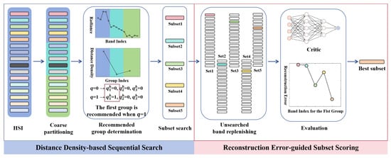
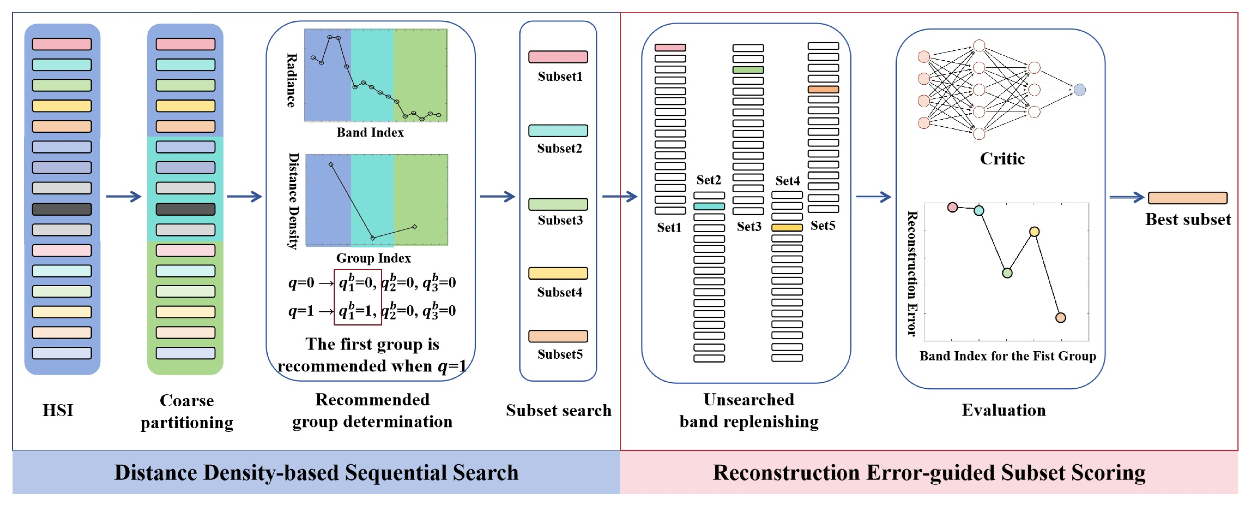
The particulars of DW-WUBS are illustrated in this section. Its flow diagrams are given in Figure 1. In the flowchart, the total number of bands $Q$, the number of groups $r$, and the number of required bands $q$ are set to 16, 3, and 1, respectively. In HSI, each polygon corresponds to a band. During coarse partitioning, bands with the same background color are grouped together. In the subset search stage, the bands in the first group are searched because this group has been identified as the recommended one. Next, unselected bands are replenished using zeros, which are represented by white polygons. Finally, the band set with the minimum RE is considered the target band. The time complexity of FFS is first analyzed, and then a strategy to enhance its efficiency is presented. Afterwards, an approach is proposed to measure the significance of selected band subsets via band reconstruction using two versions of 1-D WGAN.

Figure 1. Flowchart of the developed DW-WUBS.

2.1. Distance Density-Based Sequential Search

Several symbols utilized within the paper are explained below. Commonly, an HSI is denoted as $X={\left\{X_j\right\}}_{j=1}^Q\in R^{Q\times S}$, where $X_j$ represents the jth feature tensor, which is derived via reshaping the jth two-dimensional (2-D) spectral image into a one-dimensional (1-D) vector, and $Q$ and $S$ represent band and sample quantities, respectively. The index of bands in $X$ is sequenced.

Generally, wrapped methods demonstrate powerful capability in retrieving a band subset. To ensure the competence of the selected bands, a popular sequential search algorithm, i.e., FFS, is applied here. This approach progressively builds the recommended subsets by first identifying the 1-D feature with the minimal RE. Then, the designed predictor is used to score combinations of the current best features with the remaining bands at each iteration. The process terminates automatically when the predefined dimensionality of bands is achieved. Therefore, its time complexity is accumulated with iterated processing, which is given as

$$C_{FFS}={\sum }_{j=0}^{q-1}\left(Q-j\right),$$

(1)

Apparently, the computational burden of FFS increases with the number of bands. This makes it unsuitable for HSI applications. To boost the efficiency of band subset production, DD [37] is applied in our study because it can measure variations in bands and reduce the solution space. DD utilizes a coarse partitioning strategy, which segments $X$ into $r$ groups, with the division position $P_i$ calculated as follows:

$$P_i=\left\{\begin{array}{cc}F\left(\left[{\displaystyle \frac{Q\times \left(i-1\right)}{r}}\right]\right)+1,& 1\le i\le r\\ Q,& i=r+1\end{array}\right.,$$

(2)

where $F\left\{·\right\}$ indicates the floor operator. The gap between two contiguous bands $g_j$ can be measured by the absolute distance, calculated via

$$g_j=\left|X_{j+1}-X_j\right|,$$

(3)

The DD of the ith group $D_i$ is estimated by

$$D_i={\displaystyle \frac{\left(\sum _{j=P_{i-1}}^{P_i}{g}_j\right)}{P_i-P_{i-1}}},$$

(4)

The magnitude of DD correlates with fluctuations in band groups. A larger value indicates more complicated changes in the group and suggests that more bands should be chosen from it. Subsequently, the band quantity chosen from the ith group can be formulated as

$$q_i^b={\displaystyle \frac{q\times D_i}{\sum _{k=1}^r{D}_i}} ,$$

(5)

where $q$ indicates the band quantity chosen from the set $X$ and $q_1^b+q_2^b+\cdots +q_r^b=q$.

DD is dominantly utilized in stochastic search methods, which are incorporated into FFS to reduce the number of scores and speed up the search procedure in this paper. The proposed DD-based sequential search (DSS) maintains a similar search process to FFS but improves the step of determining the searched band group. It works in three steps.

Step 0: Initialization. Segment the HSI into $r$ groups utilizing Equation (2). Assign the recommended band quantity chosen from ith group $q_i^b$ and the dimensionality of the provisional band subset $q^{\prime }$ to zero.

Step 1: Numeration of the recommended band quantity. Aggrandize $q^{\prime }$ by 1 and calculate $q_i^b$ via Equation (5). When the dimensionality of the temporary band subset increases, the number of recommended bands in only one group changes.

Step 2: Determination of the recommended band group. Consider the band group with the incrementally recommended quantity as the suggested group. Different from former FFS-based studies, which select an element from the rest of $(Q-q^{\prime }+1)$ bands, FFS is only performed on the bands of the suggested group to build the provisional subset.

Step 3: Algorithm termination decision. If $q^{\prime }=q$, terminate the algorithm. If not, switch to Step 1.

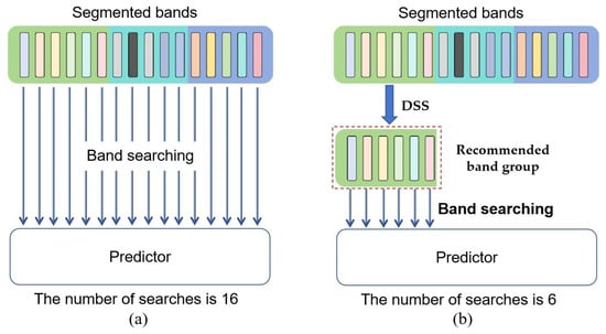
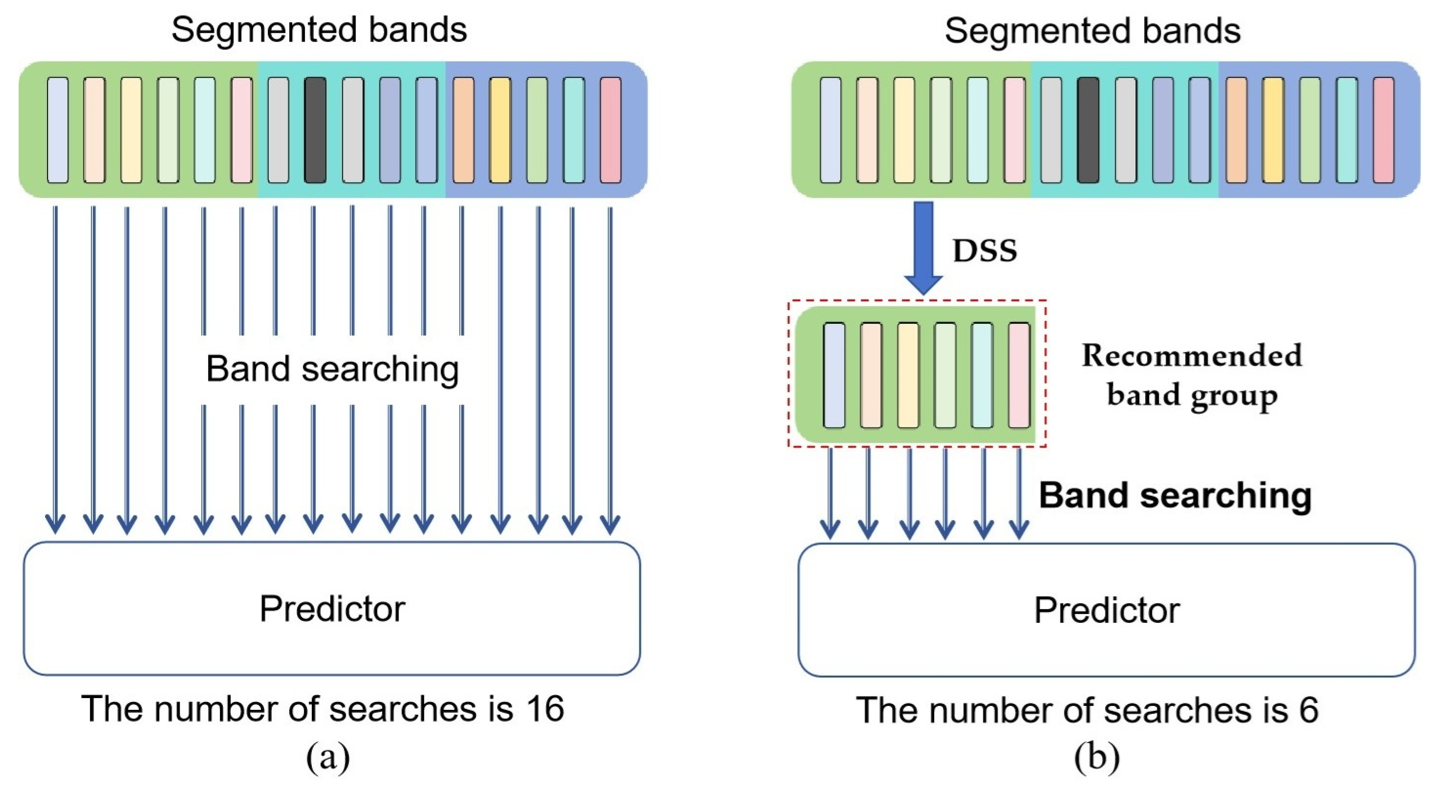
Figure 2 illustrates the superiority of our DSS. As can be seen in the above steps and Figure 2, the number of scores will decline substantially when DSS is employed. Moreover, the developed method is converted to a filtered method if $r=Q$. DSS plays a key role in equilibrating computational efficiency and band performance. The quality of chosen bands and reduced processing time can be obtained in parallel via a rational setting of group number. The time complexity of DSS is consequently described as

$$C_{DSS}={\displaystyle \frac{\sum _{j=0}^{q-1}\left(Q-j\right)}{r}},$$

(6)

Figure 2. Comparison of number of searches between (a) FFS and (b) proposed DSS.

An example to explain how DD determines the recommended band group and how DSS reduces the number of searches is given here. Let the number of required bands be $q=3$, the number of segmented groups be $r=$ 3, and the dimension of the band set be $Q=90$. Then, three band groups are obtained, with each group containing 30 bands. Assume that the relationship between $q_i^b$ and $q$ is listed in Table 1. All $q_i^b$ values are calculated via Equation (5). As can be seen in Table 1, when q increases from 0 to 1, only the number of recommended bands chosen from the first group $q_1^b$ changes. Hence, the band of the first group should be searched if $q=1$. Once q increases from 1 to 2, we observe that only $q_3^b$ increases when we compare the results of $q=1$ and $q=2$. Then, the band of the third group should be searched if $q=2$. Similarly, the band of the first group should be searched if $q=3$. Although DSS has a superposition time complexity as well, only the bands in the recommended band group should be searched when $q$ changes. Consequently, the number of searches in DSS has been greatly reduced. If we use FFS to retrieve a three-dimensional candidate subset from a 90-dimensional band set, the number of searches should be $\sum _{j=0}^{q-1}\left(Q-j\right)=90+89+88=267$. Nevertheless, this can be reduced to ${\displaystyle \frac{\sum _{j=0}^{q-1}\left(Q-j\right)}{r}}=30+30+29=89$ with the proposed DSS employed.

Table 1. An example showing the superiority of DSS.

$\mathit{q}$	${\mathit{q}}_1^{\mathit{b}}$	${\mathit{q}}_2^{\mathit{b}}$	${\mathit{q}}_3^{\mathit{b}}$
0	0	0	0
1	1	0	0
2	1	0	1
3	2	0	1

2.2. Reconstruction Error-Guided Subset Scoring

RE-guided subset scoring (RESS) involves treating the measurement of bands as a re-establishment task using a small number of bands. If the searched bands are representative, they become the core components for reliable HSI reconstruction. It needs to be noted that the structure of the predictor should be relatively simple in the wrapped algorithm, because the operating time is proportional to complexity. On that account, GAN is applied here to learn the textural information of spectral bands without a predetermined hypothesis. Traditional GANs are confronted with volatile training and mode collapse. These issues are addressed by WGAN [57] via optimizing the Earth Mover’s (EM) distance using weight clipping. This improved version is therefore adopted as the foundational framework in our study due to its reliable convergence. WGAN is composed of a generative network (G-net) and a critical network (C-net). Using competitive training, G-net and C-net can be utilized individually once fully trained. This enables the powerful yet simple C-net to be used as a predictor. In the model description below, $P_r$ and $P_g$ represent distributions of authentic samples $x$ and noise samples $z$, separately, and $C\left(·\right)$ and $G\left(·\right)$ represent the outputs of C-net and G-net, separately.

The developed DW-WUBS serves as a generic wrapped architecture. This indicates that various forms of predictors can be employed in a consistent BS workflow, provided they conform to predefined structural requirements. Fully connected networks (FCNs) and convolutional neural networks (CNNs) are two elementary forms of DL architecture. In consequence, two kinds of WGAN are designed based on FCNs and CNNs in our work, which are called WGAN-FC and WGAN-Conv, respectively.

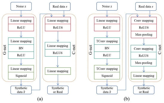
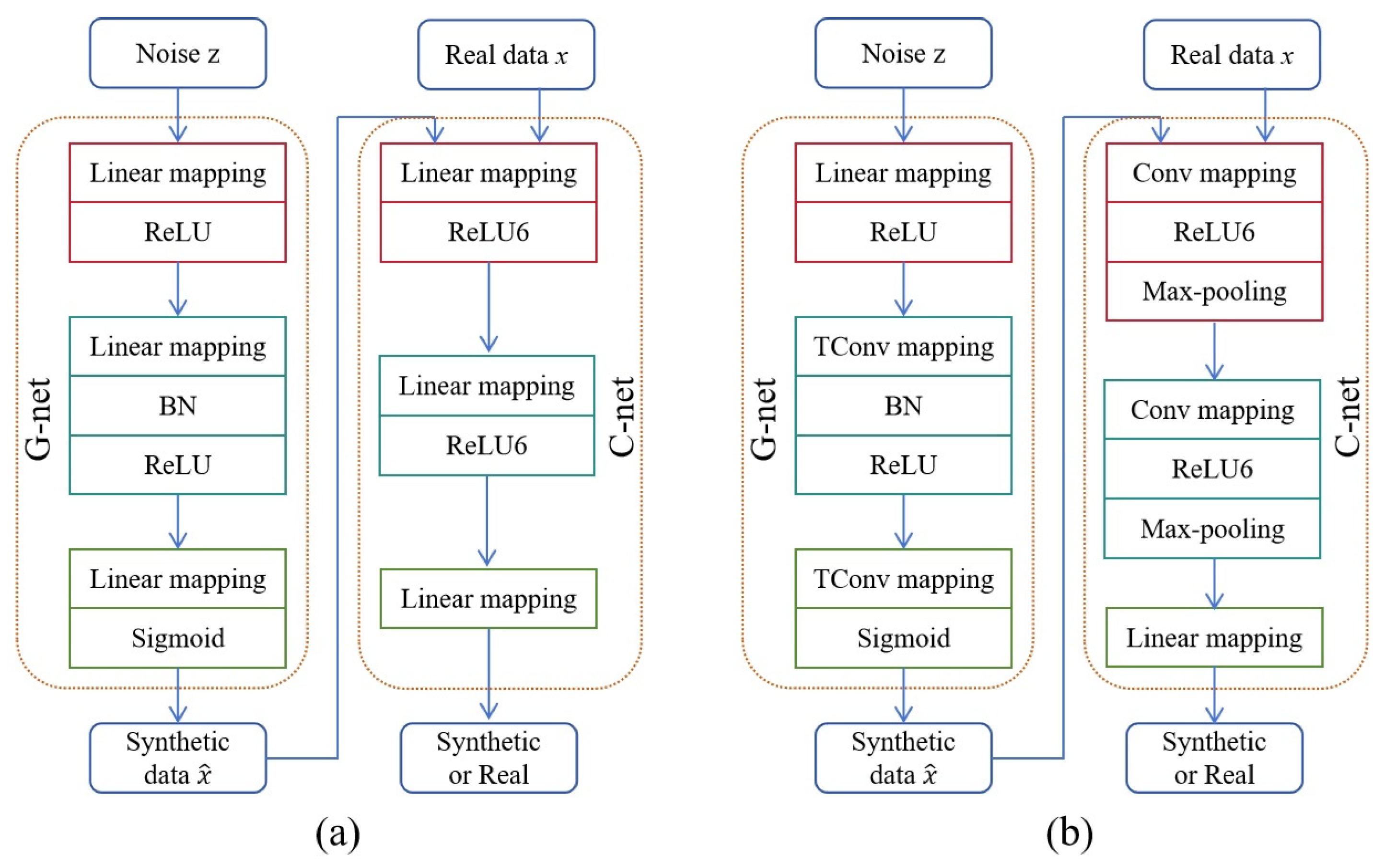
(1) WGAN-FC. For this version, both G-net and C-net are built via FC components, as exhibited in Figure 3a. G-net performs via a three-phase up-sampling process. Its inputs are Gaussian-distributed latent tensors. The architecture of G-net integrates sequential operations of linear mapping and nonlinear activation operations within each up-sampling layer. Following the dimensional expansion of latent variables via multi-layer linear mapping, G-net transforms random noises into high-dimensional representations. One-dimensional batch normalization (BN) is implemented in the second linear layer to enhance training consistency and ease initialization. Nonlinear activation modules increase model depth while maintaining computational efficiency and lowering parameters simultaneously. C-net has a structure similar to that of a multi-layer perceptron (MLP). It employs linear projection coupled with activation modules. The adopted ReLU6 activation function facilitates gradient diffusion to a limited extent, which decreases accuracy loss and promotes the convergence speed of C-net.

Figure 3. Framework of (a) WGAN-FC and (b) WGAN-Conv.

(2) WGAN-Conv. This variant is equipped with convolutional elements. Its framework is illustrated in Figure 3b. Convolution (Conv) and transposed convolution (TConv) use distinct strides in 1-D convolutional networks, enhancing training stability via selecting an appropriate stride size and preserving the crucial visual features. Max-pooling (MP) reduces the parameters of C-net and increases the computational speed and the robustness of extracted convolutional features. G-net implements linear projection once and 1-D TConv calculation twice. Nonlinear activation follows these operations. BN is employed behind the first TConv operation to avoid the network vibration. C-net consecutively uses a group of 1-D Conv, ReLU6 activation, and MP twice.

(3) Model training. WGAN training is made up of forward propagation and backpropagation. In the first stage, G-net takes 1-D noise $z$ as input and produces synthetic data $\widehat{x}$ that closely matches real samples $x$, which can be formulated by the transformation $\widehat{x}=G\left(z\right)=g(W_i^{l-1}\ast x_i^{l-1}+b)$, where $g$ is the Sigmoid function, $l$ represents the number of layers, $i$ indicates the $i$th feature tensor, and $x$ indicates the input of the ($l$ − 1)th layer. The aim is to deceive C-net by synthesizing highly authentic data. C-net acts as a quality critic, learning to point out the differences between real and generated samples through continuous adversarial training. It introduces both synthetic data $\widehat{x}$ and real data $x$ and exports their respective scores $C\left(\widehat{x}\right)= W_i^{l-1}\times {\widehat{x}}_i^{l-1}+b$ and $C\left(x\right)= W_i^{l-1}\times x_i^{l-1}+b$. In the backpropagation stage, the optimized strategy of G-net is maximizing $C\left(\widehat{x}\right)$, which is the equivalent of minimizing $-C\left(\widehat{x}\right)=-C\left(G\left(z\right)\right)$. The parameter update of G-net is then expressed as

$$\underset{G}{\mathrm{m}\mathrm{i}\mathrm{n}} L_G=-{\sum }_{z}C\left(G\left(z\right)\right),$$

(7)

The training of C-net is performed via minimality of $C\left(\widehat{x}\right)$ and maximization of $C\left(x\right)$ concurrently.

$$\underset{C}{\mathrm{m}\mathrm{i}\mathrm{n}} L_C=-{\sum }_{x}C\left(x\right)+{\sum }_{\widehat{x}}C\left(\widehat{x}\right),$$

(8)

Parameter update of WGAN is performed by optimizing Equations (7) and (8) successively using the RMSprop algorithm. As proved by Arjovsky et al. [57], Equation (8) is applied to compute the EM distance from $P_r$ to $P_g$ during training, which is then decreased by the optimization of Equation (7). Optimization ceases once the loss of C-net reaches a given threshold.

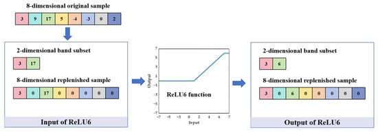
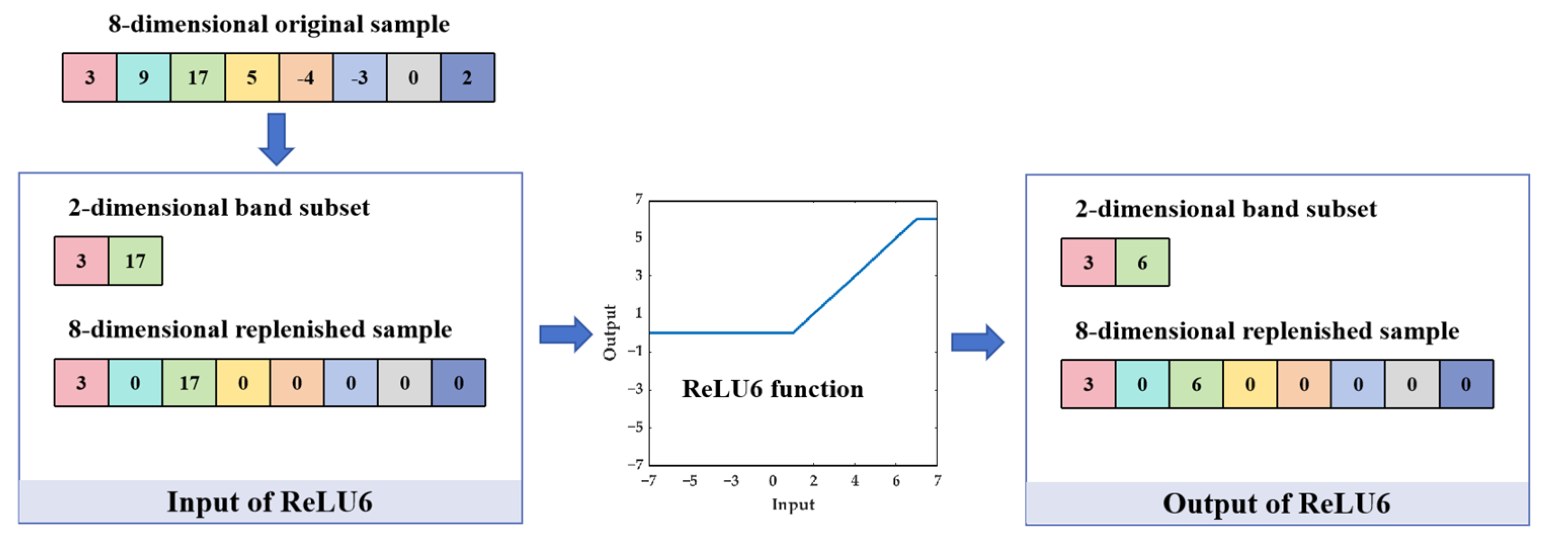
(4) Band scoring. The training samples of C-net are full-spectrum, and scoring needs the structure of input samples to match that of the training samples. To guarantee valid scoring, a replenished strategy is applied here. It utilizes the working mechanism of ReLU6, which only reacts to positive values. This strategy resets the positions of unsearched bands to zero while immobilizing the searched band values. In Figure 1, reset bands are represented by white rectangular boxes. As shown in Figure 4, if we assume that two bands are selected from an eight-dimensional set, and the unselected bands are reset to zero, it can be found that the results of the two-dimensional band subset and eight-dimensional replenished set are identical, indicating that the reset components have no effect upon scoring performance with the benefit of ReLU6. Based on this strategy, a set that can be scored is synthesized, which prevents the model from being trained multiple times. Consequently, the RE between the searched bands and the primordial data set is transformed to the EM distance from the synthesized band combination to all bands, and Equation (8) is rewritten as

$$RE=\left|{\displaystyle \frac{1}{U}}{\sum }_{i=1}^U\left[C\left(x_i^s\right)-C\left(x_i\right)\right]\right|,$$

(9)

where $x$ and $x^s$ are samples from the real and synthesized data sets, respectively; $U$ is the sample number utilized in subset scoring; and $\left|·\right|$ is the absolute operator. A smaller RE means that the searched bands are more representative and should be retained. Conversely, bands with a larger RE will be discarded.

Figure 4. Visual illustration of the reset strategy.

2.3. Implemented Procedure

The procedure implemented for DW-WUBS is listed in Algorithm 1. It primarily consists of data preprocessing, model training, DSS, and RESS. In the first stage, HSIs are normalized within a range of 0 to 1, which strengthens the reflection spectrum of objects. Subsequently, DD is computed using pixel-level samples. In the next stage, G-net and C-net are alternately trained using 1-D samples by optimizing the corresponding objective functions. The completely trained C-net is saved and subsequently applied as the predictor. In the third stage, DSS applies DD to determine the recommended band group and employs FFS to generate the suggested subset by combining a band from the recommended group with the optimal bands derived in the previous iteration. The RE of the suggested subset is computed in the final stage using RESS. The presented predictor effectively addresses the typicality of the retrieved subset. After a few iterations of the third and fourth stages, the subset with minimal RE is established, which results in the best band combination.

Algorithm 1 Procedure of DW-WUBS

Input:

- HSI:$X$;

- Terminated threshold for WGAN: $\theta$;

- Parameters of G-net and C-net: $Y_G$ and $Y_C$;

- Number of band groups: $r$;

- Target subset dimensionality: $q$;

1: Stage 1

SubStep1: Normalize the HSI $X$ and derive pixel-level samples $x$;

SubStep2: Group $X$ and compute DD via Equations (2)–(4).

2: Stage 2

SubStep1: Update $Y_G$ via Equation (7) for one time;

SubStep2: Update $Y_C$ via Equation (8) for five times;

3: Stage 3

SubStep1: Compute $q_i^b$ via Equation (5);

SubStep2: Determine the recommended band group;

SubStep3: Use FFS to search a band from recommended group.

4: Stage 4

SubStep1: Embed searched band to previous candidate subset

SubStep2: Replenish the positions of unsearched bands with zero;

SubStep3: Score the replenished set via Equation (9).

5: Primary procedure

Step1: Execute Stage1;

Step2: Repeat Stage2 until convergence and $L_C$ < $\theta$;

Step3: Save $Y_C$;

Step4: Repeat Stage3 and Stage4 until candidate subset dimensionality = $q$;

Output: Band subset with the minimal RE

2.4. Complexity Analysis

The complexity of DW-WUBS is mainly contributed to by the steps of band combination search and scoring. DD calculation (i.e., Equation (4)) is the core of the first step, providing $O\left(Q-1\right)$ complexity. Regarding band combination scoring, computation of $RE$ (i.e., Equation (9)) leads to a complexity of $O\left(2U\right)$. Each search corresponds to a scoring, but DD merely needs to be calculated once. In consequence, the time complexity of our DW-WUBS is $O\left[Q-1+2U{C}_{DSS}\right]=O[Q-1+{\displaystyle \frac{2U\sum _{j=0}^{q-1}\left(Q-j\right)}{r}}]$.

3. Experiments

3.1. Data Set

This paper presents the experimental validation of our DW-WUBS utilizing three noted HSI data sets via image classification tasks. Detailed information regarding the number of labeled samples is listed in Table 2.

Table 2. Number of labeled samples in different HSI band sets.

No.	PaviaU		Botswana		Pavia Center
	Class	Number	Class	Number	Class	Number
C1	Asphalt	6631	Water	270	Water	65,971
C2	Meadows	18,649	Hippo grass	102	Forests	7598
C3	Gravel	2099	Floodplain grass l	251	Asphalt	3090
C4	Forests	3064	Floodplain grass 2	215	Bricks	2685
C5	Sheets	1345	Reeds	269	Bitumen	6584
C6	Bare area	5029	Riparian	269	Tiles	9248
C7	Bitumen	1330	Firescar	259	Shadows	7287
C8	Bricks	3682	Island interior	203	Meadows	42,826
C9	Shadows	947	Acacia woodlands	314	Bare area	2803
C10			Acacia shrub lands	248
C11			Acacia grasslands	305
C12			Short mopani	181
C13			Mixed mopani	268
C14			Expose soils	95
Totality		42,776		3249		148,152

(1)

PaviaU data set. The first data set is composed of ROSIS images acquired at Pavia University in Italy, with dimensions of 610 × 340 pixels. The covered area comprises nine types of interest. Following the elimination of useless components, 103 channels are retained.

(2)

Botswana data set. The second data set comprises Hyperion images of the Okavango Delta region of Botswana, taken by NASA EO-1. It has 800 × 700 pixels and 145 bands.

(3)

Pavia Center data set. The third HSI is of the Pavia Center region of Italy, collected by the ROSIS system. This HSI, with dimensions of 1096 × 715 pixels and 102 channels after noise elimination, contains nine land cover categories.

3.2. Competitor

The proposed DW-WUBS is competed with ten unsupervised BS methods, including the four reconstruction-based methods introduced in Section 1, i.e., AEFS [44], S-AEBS [11], BS-Net [46], and REFS [15], and six state-of-the-art methods, i.e., feature dependency-based unsupervised feature selection (DUFS) [58], spectral–spatial cross-dimensional attention network (SSANet) [59], neighborhood grouping normalized matched filter (NGNMF) [60], dual attention reconstruction network (DARecNet) [61], sample latent feature associated low-rank subspace clustering (SLFLRSC) [62], and low-rank tensor based smooth representation learning (LTSRL) [63]. AEFS, S-AEBS, and BS-Net are DL-based methods as well. DUFS explores the pairwise dependence of features to select bands based on information theory. In SSANet, interactions between spectral and spatial dimensions are applied to measure the discrimination of subsets. NGNMF selects a band group via a novel matched filter to save spectral information. DARecNet presents a dual attention mechanism to explore the long-range nonlinear contextual information in spatial and spectral dimensions. SLFLRSC combines entropy rate segmentation and Laplacian eigenmaps to express sample–spatial consistency. LTSRL uses a self-representation matrix and a weighted low-rank tensor restriction to learn higher-level information. Moreover, classification results from all bands are considered as the baseline. The parameters of the aforesaid methods are derived via the primordial theses, which are shown in Table 3. As for our method, the RMSprop algorithm is utilized to train WGAN-GP with a 3 × 10⁻⁴ -learning rate and 128-batch size. The termination θ is 2 × 10⁻⁴ for all data sets. The number of band groups r is searched from {2, 3, …, 10, 15}. Moreover, FCN- and CNN-based predictors lead to two editions of the BS algorithm, which are referred to as DW-WUBS-FC and DW-WUBS-Conv, respectively. Any arguments are gained on Pavia Center data set and applied to other data sets. All the samples are applied to generate a band subset for various BS algorithms.

Table 3. Parameters used in different UBS methods.

Method	Parameter	Value
AEFS	Size of hidden layer $\epsilon$, and regularization factors $\alpha$ and $\beta$	128, 10−1, 10
S-AEBS	Size of hidden layer $\epsilon$, regularization factors $\alpha$ and $\beta$, and the number of groups $r$	Half the size of the input layer, 10−4, 10−1, 4
BS-Net	Regularization factor $\alpha$, learning rate $\eta$, and iteration number $n$	10−2, 2 $\times$ 10−3, 102
REFS	Feature coeficient $s$ and graph coeficient $p$	10−4, 0.5
DUFS	Regularization factors $\alpha$, $\beta$, and $\lambda$	1, 10, 10
SSANet	Regularization parameter $\lambda$	10−1
NGNMF	-	-
DARecNet	-	-
SLFLRSC	Regularization factors $\alpha$, $\beta$, $\lambda$, and $\tau$	102, 1, 102, 102
LTSRL	Regularization factors $\alpha$, $\beta ,$ and $\lambda$	10−3, 10−1, 20
DW-WUBS-FC	The number of groups $r$	2
DW-WUBS-Conv	The number of groups $r$	3

3.3. Setting

The use of retrieved bands for classification serves as the principal pattern to assess the performance of BS. In the experiments, we apply support vector machine (SVM) and k-nearest neighbors (KNN) classifiers on three distinguishing data sets, with their parameters derived via four-fold cross-validation. We randomly choose 15% of the samples for training and use the remainder for testing. Each method experiences twelve repeated assessments to guarantee reliability, with the ultimate results calculated as the average. We employ three classical assessment indicators to analyze the algorithmic performance, i.e., overall accuracy (OA), kappa coefficient (KC), and mean accuracy (MA). The number of chosen bands is set according to {3, 6, …, 30} to investigate the effects of varied spectral quantities. Algorithm assessment is implemented in MATLAB R2022b operating on an AMD Ryzen-7-7840H processor running at 3.80 GHz with 16 GB of RAM. The parameters of WGAN-FC and WGAN-Conv designed in this paper are listed in Table 4. DW-WUBS is carried out on PyTorch 2.1.2, and an NVIDIA GeForce 4060 GPU with 8 GB of memory is adopted for acceleration.

Table 4. Parameters of WGAN-FC and WGAN-Conv for PaviaU data set.

Model	WGAN-FC			WGAN-Conv
Module	Layer	Hidden Size	Activation	Layer	Kernel	Activation
G-net	Input	25	-	Input	51	ReLU
	FC1	64	ReLU	FC1	800	ReLU
	FC2	128	ReLU (BN)	View1	25 $\times$ 1 $\times$ 32	-
	FC3	103	Sigmoid	TConv1	3 $\times$ 1 $\times$ 32	ReLU (BN)
	-	-	-	TConv2	3 $\times$ 1 $\times$ 1	Sigmoid
C-net	Input	103	-	Input	103
	FC1	256	ReLU6	Conv1	3 $\times$ 1 $\times$ 32	ReLU6
	FC2	128	ReLU6	MP1	2 $\times$ 1	-
	FC3	1	-	Conv2	3 $\times$ 1 $\times$ 16	ReLU6
				MP2	2 $\times$ 1	-
	-	-	-	FC1	1	-

3.4. Analysis of Classification Results

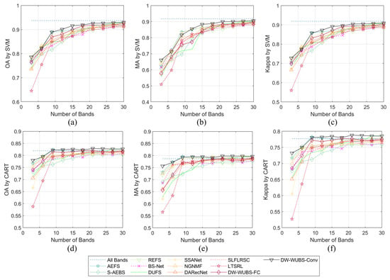
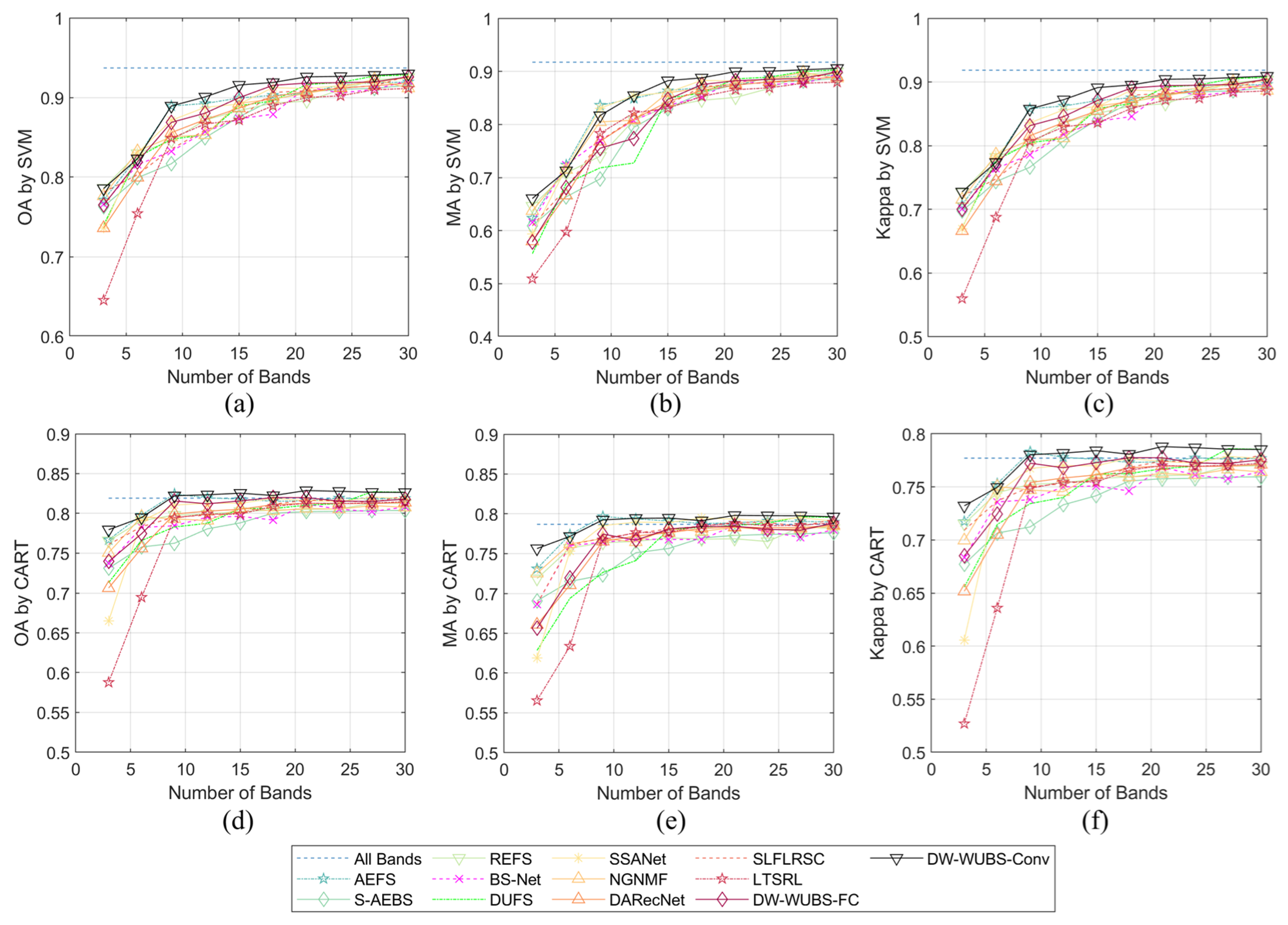
Using SVM and CART classifiers and ten advanced UBS algorithms, the proposed DW-WUBS is examined in two ways: OA, MA, and KC curves in opposition to diverse band amounts and the average of OA, MA, and KC values within the scope of 3 to 30 bands.

(1) Accuracy curves for the Pavia University region. The accuracy curves of Pavia University employing two classifiers are demonstrated in Figure 5. These curves show that the classification accuracy of all methods gradually becomes steady as the dimensionality of chosen subsets is augmented, testifying to the redundancy of HSIs and the necessity of BS. Moreover, the proposed DW-WUBS obtains preferable classification results with both classifiers. When the CART classifier is applied, only the accuracies of DW-WUBS-Conv and AEFS surpass those of the baseline. For DW-WUBS-FC, its performance is weaker than that of DW-WUBS-Conv, but it outperforms the remaining algorithms. For the OAs of the CART classifier, if nine-dimensional band subsets are selected, our DW-WUBS-Conv exceeds REFS, LTSRL, and DUFS by 3.02%, 0.34%, and 4.83%, respectively. This is due to the proposed method taking advantage of nonlinear spectral characteristics. Moreover, despite both S-AEBS and DW-WUBS-Conv using DD to optimize subset retrieval, their classification performance differs significantly, which may be attributed to two factors. One is the powerful scoring ability of the designed C-net, and the other is the robustness of DW-WUBS to hyperparameters. Another phenomenon is that DW-WUBS attains the optimal OA, MA, and KC on both SVM and CART—for instance, 92.98% OA on SVM and 82.87% OA on CART. Whole BS algorithms are inferior to the baseline on SVM, but our method takes a leadership role in almost all cases. All situations show that DW-WUBS is effective in choosing a reliable subset.

Figure 5. Classification results on PaviaU scene with various numbers of bands. (a) OA gained by SVM. (b) MA gained by SVM. (c) KC gained by SVM. (d) OA gained by CART. (e) MA gained by CART. (f) KC gained by CART.

(2) Accuracy curves for Botswana Region. The accuracy tendencies of all BS algorithms on this scene with varied amounts of chosen bands are displayed in Figure 6. As we can conclude from Figure 6d–f, when CART is used, DW-WUBS-FC gains preferable results to the baseline via choosing fewer bands, i.e., 81.88% OA, 83.09% MA, and 80.87% KC with 15, 9, and 15 chosen bands, respectively. As shown in Figure 6a–c, S-AEBS ranks first on SVM when the dimensionality of the chosen subsets surpasses 24. But its results gradually decrease as the number of recommended bands decreases, whereas our DW-WUBS-FC achieves better performance. This testifies to the fact that the proposed method chooses bands without losing key information, even when only a small number of bands are required, which demonstrates the potential of the proposed algorithm to significantly reduce storage requirements. When the CART classifier is applied, it is found that the designed algorithms generally achieve higher classification performance when more bands are selected. Because DW-WUBS is a search-based framework, a larger solution space with more features tends to yield superior performance. In consequence, our method is apt to retrieve the top bands from the incremental dimensionality of band subsets. This demonstrates the retrieval capability of the presented DSS.

Figure 6. Classification results on Botswana scene with various numbers of bands. (a) OA gained by SVM. (b) MA gained by SVM. (c) KC gained by SVM. (d) OA gained by CART. (e) MA gained by CART. (f) KC gained by CART.

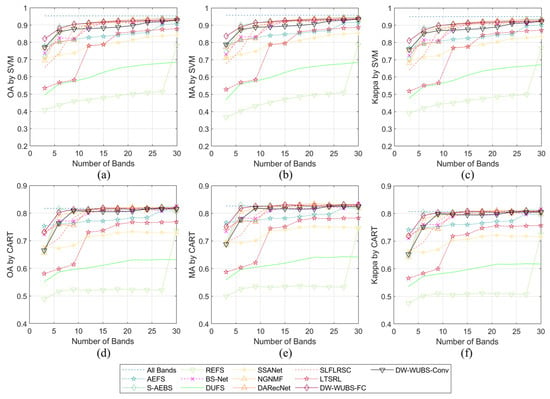
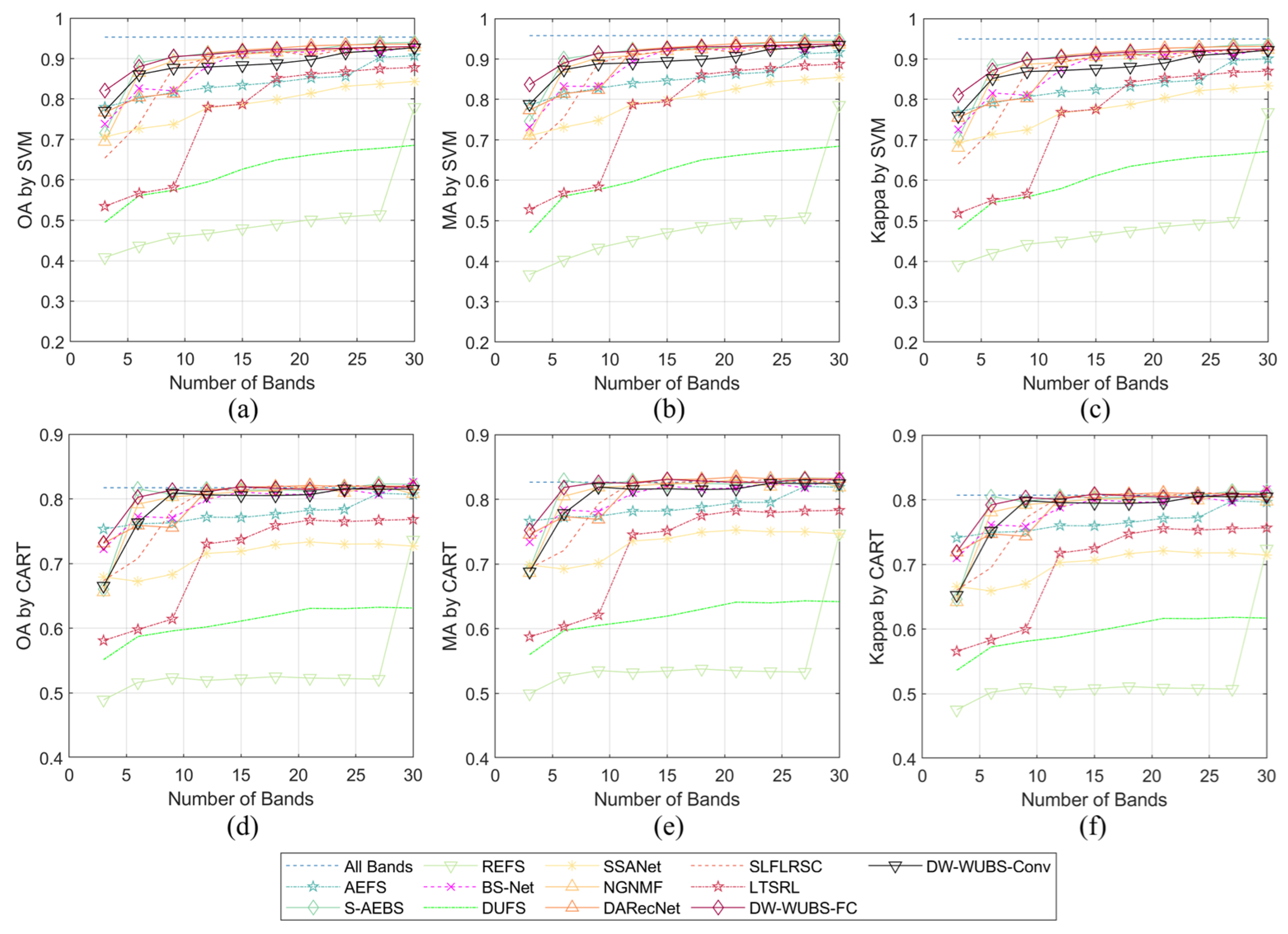
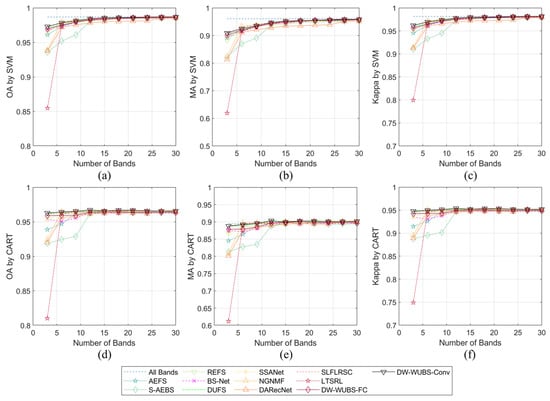
(3) Accuracy curves for the Pavia Center region. The classification performance evaluated via SVM and CART using different bands is exhibited in Figure 7. By observing the figures, two phenomena can be summarized. Firstly, the majority of BS methods obtain almost identical OA, MA, and KC values. One possible interpretation for this matter is that the hyperparameters of BS methods are determined using this data set, and all methods show their best performance when valuable bands are selected with optimal parameterization. Even so, our DW-WUBS achieves the preferred classification results, although the discrepancy is not very evident. Secondly, the classification accuracies produced by our approach are relatively stable across varying numbers of bands on both classifiers, which should be attributed to its ability to recognize underlying band-combining information. As for the results of the CART classifier, the peak mean accuracy using the 12 bands chosen via DW-WUBS-Conv exceeds the baseline (i.e., all bands) by 0.92% in the classification task. Under the same subset dimension, DW-WUBS-Conv, BS-net, and SSANet also overmatch the baseline because they identify effective spectral information from complex HSI via a specific deep network architecture. To sum up, the findings presented herein indicate that DW-WUBS is consistent in achieving stabilized and outstanding results across various HSIs. This shows the robustness of our approach to BS.

Figure 7. Classification results on Pavia Center scene with various numbers of bands. (a) OA gained by SVM. (b) MA gained by SVM. (c) KC gained by SVM. (d) OA gained by CART. (e) MA gained by CART. (f) KC gained by CART.

(4) Averaged classification indicators. Table 5 lists the averaged OA, MA, and KC of various UBS approaches on the three HSIs. The classification indicators, which are marked in bold font, represent the top performance. As shown in the table, DW-WUBS outperforms other advanced BS algorithms in OA, MA, and KC. As DW-WUBS incorporates RE into band importance analysis to reject redundancy, it is superior to DUFS, NGNMF, SSANet, SLFLRSC, and LTSRL via retrieving a greater number of typical bands from the original HSIs in classification. Unlike REFS, which uses a linear RE criterion, the proposed method considers both linear and nonlinear characteristics in data reconstruction. This leads to a preferable classification performance for our method. For S-AEBS, it individually applies DD to perform a deep examination of changes in the spectrum. But our method combines DD and a sequential search to accomplish more detailed retrieval, which is more valid when handling noisy bands and choosing the most promising bands. AEFS, DARecNet, and BS-net explore the best weight factors for diverse band combinations by applying an embedded data reconstruction module. In contrast, our DW-WUBS unifies data reconstruction, DD, and band search in a wrapped architecture whose performance outperforms the two above DL algorithms. Furthermore, Table 5 shows that DW-WUBS-Conv performs slightly worse than DW-WUBS-FC on the Botswana data set. The differences between DW-WUBS-Conv and DW-WUBS-FC are reflected in two aspects: the architecture of the evaluators and the number of segmented groups $r$. In our study, all arguments are achieved based on the Pavia Center data set and are applied to other data sets for a fair comparison of the various methods. The number of segmented groups is set to 2 and 3 for DW-WUBS-FC and DW-WUBS-Conv, respectively. We hypothesize that the discrepancy between DW-WUBS-Conv and DW-WUBS-FC on the Botswana data set is possibly due to the number of segmented groups $r$, as the ability of the DSS and WGAN-FC or WGAN-Conv to cooperate is slightly influenced by the number of segmented groups.

Table 5. Averaged classification indicators within the scope of 3 to 30 bands.

Scene	Indicator	AEFS	S-AEBS	REFS	BS-Net	DUFS	SSANet	NGNMF	DARecNet	SLFLRSC	LTSRL	DW- WUBS-FC	DW- WUBS-Conv
SVM classifier
PaviaU	OA	88.40	86.45	87.62	86.74	87.42	88.00	87.55	87.17	87.21	85.00	88.30	89.44 1
	MA	83.12	79.78	80.95	81.35	79.77	82.94	82.42	80.79	81.15	78.87	80.64	84.24
	KC	85.13	82.66	84.12	83.02	83.89	84.70	84.07	83.55	83.59	80.95	84.98	86.43
Botswana	OA	84.20	89.88	50.45	87.86	61.99	78.61	88.78	88.83	86.84	75.85	90.62	88.17
	MA	85.28	90.95	49.08	88.56	61.75	79.61	89.75	89.57	87.91	76.43	91.54	89.28
	KC	83.28	89.24	48.88	87.12	60.48	77.48	88.09	88.14	86.09	74.72	90.00	87.43
Pavia center	OA	98.09	97.35	98.20	98.13	98.27	98.16	98.00	97.56	98.31	97.12	98.18	98.36
	MA	94.00	92.12	94.03	94.01	94.25	94.08	93.63	92.22	94.47	91.47	94.21	94.50
	KC	97.31	96.21	97.46	97.36	97.55	97.41	97.18	96.56	97.62	95.98	97.43	97.68
CART classifier
PaviaU	OA	81.14	78.33	79.97	79.15	79.38	79.81	79.70	80.13	80.18	77.37	80.46	81.77
	MA	78.34	75.05	76.42	76.29	75.19	77.02	77.09	77.40	77.14	74.53	76.15	78.91
	KC	76.84	73.61	75.44	74.56	74.77	75.36	75.19	75.33	75.73	72.69	75.98	77.54
Botswana	OA	77.79	80.00	54.00	79.38	60.93	71.20	79.41	79.76	78.88	70.87	80.60	79.07
	MA	78.93	81.35	55.14	80.40	61.90	73.15	80.80	81.07	80.00	72.11	81.93	80.22
	KC	76.64	78.94	52.61	78.29	59.49	69.93	78.33	78.69	77.79	69.59	79.55	77.98
Pavia Center	OA	95.94	95.16	96.32	96.07	96.51	96.31	96.04	95.75	96.41	94.97	96.24	96.57
	MA	88.68	87.28	89.46	89.03	89.77	89.28	88.89	88.26	89.64	87.04	89.29	89.87
	KC	94.31	93.24	94.83	94.48	95.09	94.82	94.45	94.05	94.96	93.09	94.72	95.18

¹ The classification indicators marked in bold font represent the top performance.

Overall, DW-WUBS performs best on all data sets. The classification indicators demonstrate that DW-WUBS is able to access a group of representative and informative bands. This is in conformity with the objective of BS.

3.5. Ablation Study

DW-WUBS integrates DSS with RESS to retrieve the top subset. DSS is implemented via the collaborative employment of DD and FFS. In RESS, RE is computed via C-net. Ablation studies were conducted to evaluate the contributions of the distinct components in the proposed architecture. The valid configurations of module interactions in DW-WUBS are expressed as follows:

(1)

Basic algorithm (B). The variant without DD and C-net is considered the basic algorithm. This version employs FFS to search bands, which are subsequently scored via a fundamental mean bias error (MBE) loss function. In this case, the scoring criteria, i.e., Equation (9), is converted to

$$RE=\left|{\displaystyle \frac{1}{U}}{\sum }_{i=1}^U\left(x_i^s-x_i\right)\right|,$$

(10)

(2)

B + FCC and B + ConvC. The variants consist of a basic algorithm and FC C-net (FCC) and Conv C-net (ConvC), respectively.

(3)

B + D. The variant consists of a basic algorithm and DD.

(4)

DW-WUBS. The developed algorithm.

Table 6 exhibits the classification performance of variants of DW-WUBS-FC and DW-WUBS-Conv provided by the SVM. The dimensionalities of the band subsets q are set to {3, 9, 18, 30}. The parametric settings are identical to those of the preceding experiment. The classified difference of B + D between DW-WUBS-FC-related and DW-WUBS-Conv-related methods is caused by the different numbers of groups. As we can see in the results, the OAs of the basic algorithm across all data sets are absolutely mediocre. Nevertheless, B + FCC, B + ConvC, and B + D show enhanced classification performance across three HSIs when DD and C-net are applied, compared with the basic algorithm. For example, B + ConvC performs best on the Botswana scene if 18 bands are chosen. B + D outperforms the other algorithms on the PaviaU scene with three chosen bands. This demonstrates the importance of recognizing the recommended band group and capturing the underlying and higher-level structure. For our DW-WUBS, it obtains the best performance in most cases, which illustrates that the proposed algorithm strikes the best balance between the different modules via combining them to achieve optimal results in various scenes. Depending on the aforesaid findings, the diverse constituents work best with each other in the designed DW-WUBS architecture.

Table 6. OAs of ablation study for DW-WUBS on different HSI cubes.

Scene	$\mathit{q}$	DW-WUBS-FC-Related Method				DW-WUBS-Conv-Related Method
		B	B + FCC	B + D	DW- WUBS-FC	B	B + ConvC	B + D	DW- WUBS-Conv
PaviaU	3	66.32	75.96	77.55 2	77.11	66.32	67.11	79.30	78.99
	9	75.64	87.29	79.68	87.55	75.64	85.20	83.00	89.59
	18	79.65	90.64	84.70	92.22	79.65	89.61	87.22	92.56
	30	88.09	93.00	90.31	93.28	88.09	93.54	90.28	93.57
Botswana	3	43.83	67.28	60.48	82.04	43.83	67.73	67.71	77.02
	9	82.27	86.51	84.89	90.49	82.27	85.24	82.26	87.69
	18	86.06	86.93	88.39	92.27	86.06	90.36	87.39	88.78
	30	91.25	89.51	91.53	92.98	91.25	92.36	88.85	92.71
Pavia Center	3	85.50	88.18	93.84	96.97	85.50	95.59	97.09	97.31
	9	87.51	97.63	96.25	97.97	87.51	97.54	98.04	98.14
	18	89.90	98.19	97.78	98.50	89.90	97.69	98.27	98.60
	30	94.05	98.44	98.19	98.59	94.05	98.24	98.38	98.70

² The OAs marked in bold font represent the top performance.

3.6. Analysis for Hyperparameter Sensitivity

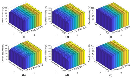
The hyperparameter r is responsible for significant band group identification in the feature search term. Its effect on DW-WUBS is explored in this section. The values of the hyper-parameter r and the number of chosen bands q are changed from the sets of {2, 3, …, 10, 15} and {3, 6, …, 30}, respectively. Figure 8 shows the OAs processed via SVM on the three scenes. It can be observed that the OAs of DW-WUBS remain relatively stationary on the first and the third data sets as the parameter r is varied. Striking differences arise in the results of the Botswana data set when a small number of bands is chosen. As shown in Figure 8a,b, the OA values are apt to reduce with the increased parameter r. This may be because a greater value of r makes the SFS term more susceptible to a local optimal solution, which brings about an attenuation in classification accuracy.

Figure 8. Over-accuracy variations of DW-WUBS versus various r values. (a) OA of DW-WUBS-FC on PaviaU scene. (b) OA of DW-WUBS-Conv on PaviaU scene. (c) OA of DW-WUBS-FC on Botswana scene. (d) OA of DW-WUBS-Conv on Botswana scene. (e) OA of DW-WUBS-FC on Pavia Center scene. (f) OA of DW-WUBS-Conv on Pavia Center scene.

In brief, the parameter r does not significantly affect our approach for the majority of data sets. However, because DW-WUBS-FC obtains optimal classification results on PaviaU, Botswana, and Pavia Center data sets if r is 7, 2, and 2, respectively, and for DW-WUBS-Conv, its top OAs are achieved on the three scenes with r values of 6, 7, and 3, respectively, a smaller value of r is recommended when applying our method.

4. Conclusions

In this paper, a new WUBS algorithm is proposed from the standpoint of image reconstruction. It starts by employing a coarse partitioning strategy for HSI to divide it into several band groups. Next, a DD technique is incorporated into a sequential search framework for local density calculation. The combination of DD and SFS minimizes the number of evaluations of band combinations, thereby decreasing computational complexity. Then, two versions of 1-D WGAN are designed and trained via pixel-scale samples. Finally, the RE obtained by the well-trained critic is proposed as a scoring criterion to explore higher-level and underlying features between bands. Experiments on three real HSIs illustrate the effectiveness of DW-WUBS over state-of-the-art algorithms.

References

- Zhang, Z.; Ni, W.; Quegan, S.; Chen, J.; Gong, P.; Rodriguez, L.C.E.; Guo, H.; Shi, J.; Liu, L.; Li, Z.; et al. Deforestation in Latin America in the 2000s predominantly occurred outside of typical mature forests. Innovation 2024, 5, 100610. [Google Scholar] [CrossRef] [Scilit]
- Meng, S.L.; Pang, Y.; Zhang, Z.J.; Jia, W.; Li, Z.Y. Mapping Aboveground Biomass using Texture Indices from Aerial Photos in a Temperate Forest of Northeastern China. Remote Sens. 2016, 8, 230. [Google Scholar] [CrossRef] [Scilit]
- Guo, A.T.; Huang, W.J.; Qian, B.X.; Ye, H.C.; Jiao, Q.J.; Cheng, X.Z.; Ruan, C. A hybrid model coupling PROSAIL and continuous wavelet transform based on multi-angle hyperspectral data improves maize chlorophyll retrieval. Int. J. Appl. Earth Obs. Geoinf. 2024, 132, 104076. [Google Scholar] [CrossRef] [Scilit]
- Zhang, M.Y.; Gong, M.G.; Mao, Y.S.; Li, J.; Wu, Y. Unsupervised Feature Extraction in Hyperspectral Images Based on Wasserstein Generative Adversarial Network. IEEE Trans. Geosci. Remote Sens. 2019, 57, 2669–2688. [Google Scholar] [CrossRef] [Scilit]
- Hennessy, A.; Clarke, K.; Lewis, M. Generative Adversarial Network Synthesis of Hyperspectral Vegetation Data. Remote Sens. 2021, 13, 2243. [Google Scholar] [CrossRef] [Scilit]
- Huan, R.; Pan, Y. Decision fusion strategies for SAR image target recognition. IET Radar Sonar Navig. 2011, 5, 747–755. [Google Scholar] [CrossRef] [Scilit]
- Liu, F.; Jiao, L.; Tang, X. Task-Oriented GAN for PolSAR Image Classification and Clustering. IEEE Trans. Neural Netw. Learn. Syst. 2019, 30, 2707–2719. [Google Scholar] [CrossRef] [Scilit]
- Chang, C.I.; Du, Q.; Sun, T.L.; Althouse, M.L.G. A joint band prioritization and band-decorrelation approach to band selection for hyperspectral image classification. IEEE Trans. Geosci. Remote Sens. 1999, 37, 2631–2641. [Google Scholar] [CrossRef] [Scilit]
- Li, S.Y.; Peng, B.D.; Fang, L.; Zhang, Q.; Cheng, L.; Li, Q. Hyperspectral Band Selection via Difference Between Intergroups. IEEE Trans. Geosci. Remote Sens. 2023, 61, 5503310. [Google Scholar] [CrossRef] [Scilit]
- Sun, H.; Ren, J.; Zhao, H.; Yuen, P.; Tschannerl, J. Novel Gumbel-Softmax Trick Enabled Concrete Autoencoder With Entropy Constraints for Unsupervised Hyperspectral Band Selection. IEEE Trans. Geosci. Remote Sens. 2021, 60, 5506413. [Google Scholar] [CrossRef] [Scilit]
- Tschannerl, J.; Ren, J.; Zabalza, J.; Marshall, S. Segmented Autoencoders for Unsupervised Embedded Hyperspectral Band Selection. In Proceedings of the 7th European Workshop on Visual Information Processing (EUVIP), Tampere, Finland, 26–28 November 2018. [Google Scholar]
- Wang, Q.; Zhang, F.; Li, X. Hyperspectral Band Selection via Optimal Neighborhood Reconstruction. IEEE Trans. Geosci. Remote Sens. 2020, 58, 8465–8476. [Google Scholar] [CrossRef] [Scilit]
- Zhao, Z.; He, X.F.; Cai, D.; Zhang, L.J.; Ng, W.; Zhuang, Y.T. Graph Regularized Feature Selection with Data Reconstruction. IEEE Trans. Knowl. Data Eng. 2016, 28, 689–700. [Google Scholar] [CrossRef] [Scilit]
- Wen, J.; Han, N.; Fang, X.Z.; Fei, L.K.; Yan, K.; Zhan, S.H. Low-Rank Preserving Projection Via Graph Regularized Reconstruction. IEEE Trans. Cybern. 2019, 49, 1279–1291. [Google Scholar] [CrossRef] [Scilit]
- Li, J.; Tang, J.; Liu, H. Reconstruction-based Unsupervised Feature Selection: An Embedded Approach. In Proceedings of the 26th International Joint Conference on Artificial Intelligence, Melbourne, Australia, 19–25 August 2017; pp. 2159–2165. [Google Scholar]
- Yang, S.; Zhang, R.; Nie, F.; Li, X. Unsupervised Feature Selection Based on Reconstruction Error Minimization. In Proceedings of the IEEE International Conference on Acoustics, Speech and Signal Processing (ICASSP), Brighton, UK, 12–17 May 2019. [Google Scholar]
- Zhang, X.; Xie, W.Y.; Li, Y.S.; Lei, J.; Du, Q.; Yang, G. Rank-Aware Generative Adversarial Network for Hyperspectral Band Selection. IEEE Trans. Geosci. Remote Sens. 2022, 60, 5521812. [Google Scholar] [CrossRef] [Scilit]
- Wang, D.Y.; Vinson, R.; Holmes, M.; Seibel, G.; Bechar, A.; Nof, S.; Tao, Y. Early Detection of Tomato Spotted Wilt Virus by Hyperspectral Imaging and Outlier Removal Auxiliary Classifier Generative Adversarial Nets (OR-AC-GAN). Sci. Rep. 2019, 9, 4377. [Google Scholar] [CrossRef] [Scilit] [PubMed]
- Geng, X.; Sun, K.; Ji, L.; Zhao, Y. A Fast Volume-Gradient-Based Band Selection Method for Hyperspectral Image. IEEE Trans. Geosci. Remote Sens. 2014, 52, 7111–7119. [Google Scholar] [CrossRef] [Scilit]
- Ji, L.; Zhu, L.; Wang, L.; Xi, Y.; Geng, X. FastVGBS: A Fast Version of the Volume-Gradient-Based Band Selection Method for Hyperspectral Imagery. IEEE Geosci. Remote Sens. Lett. 2020, 18, 514–517. [Google Scholar] [CrossRef] [Scilit]
- Zhu, G.; Huang, Y.; Li, S.; Tang, J.; Liang, D. Hyperspectral Band Selection via Rank Minimization. IEEE Geosci. Remote Sens. Lett. 2017, 14, 2320–2324. [Google Scholar] [CrossRef] [Scilit]
- He, W.; Zhang, H.; Shen, H.; Zhang, L. Hyperspectral Image Denoising Using Local Low-Rank Matrix Recovery and Global Spatial–Spectral Total Variation. IEEE J. Sel. Top. Appl. Earth Obs. Remote Sens. 2018, 11, 713–729. [Google Scholar] [CrossRef] [Scilit]
- Martinez-Uso, A.; Pla, F.; Sotoca, J.M.; García-Sevilla, P. Clustering-Based Hyperspectral Band Selection Using Information Measures. IEEE Trans. Geosci. Remote Sens. 2007, 45, 4158–4171. [Google Scholar] [CrossRef] [Scilit]
- Zhang, M.; Ma, J.; Gong, M. Unsupervised Hyperspectral Band Selection by Fuzzy Clustering With Particle Swarm Optimization. IEEE Geosci. Remote Sens. Lett. 2017, 14, 773–777. [Google Scholar] [CrossRef] [Scilit]
- Wang, Q.; Li, Q.; Li, X. A Fast Neighborhood Grouping Method for Hyperspectral Band Selection. IEEE Trans. Geosci. Remote Sens. 2020, 59, 5028–5039. [Google Scholar] [CrossRef] [Scilit]
- Guo, J.; Guo, Y.; Kong, X.; He, R.; Quo, Y. Unsupervised feature selection with ordinal locality. In Proceedings of the IEEE International Conference on Multimedia and Expo (ICME), Hong Kong, China, 10–14 July 2017. [Google Scholar]
- Wang, Q.; Li, Q.; Li, X. Hyperspectral Band Selection via Adaptive Subspace Partition Strategy. IEEE J. Sel. Top. Appl. Earth Obs. Remote Sens. 2019, 12, 4940–4950. [Google Scholar] [CrossRef] [Scilit]
- Jia, S.; Tang, G.; Zhu, J.; Li, Q. A Novel Ranking-Based Clustering Approach for Hyperspectral Band Selection. IEEE Trans. Geosci. Remote Sens. 2015, 54, 88–102. [Google Scholar] [CrossRef] [Scilit]
- Wang, Q.; Zhang, F.; Li, X. Optimal Clustering Framework for Hyperspectral Band Selection. IEEE Trans. Geosci. Remote Sens. 2018, 56, 5910–5922. [Google Scholar] [CrossRef] [Scilit]
- Yang, C.; Hou, B.; Guo, X.; Ren, B.; Chanussot, J.; Wang, S.; Jiao, L. Reconstruction Error-Based Decomposition Feature Selection for PolSAR Image. IEEE Trans. Geosci. Remote. Sens. 2022, 60, 5216719. [Google Scholar] [CrossRef] [Scilit]
- Gao, H.; Zhang, Q.K. Alpha evolution: An efficient evolutionary algorithm with evolution path adaptation and matrix generation. Eng. Appl. Artif. Intell. 2024, 137, 109202. [Google Scholar] [CrossRef] [Scilit]
- Sekara, T.B.; Matausek, M. Optimization of PID Controller Based on Maximization of the Proportional Gain Under Constraints on Robustness and Sensitivity to Measurement Noise. IEEE Trans. Autom. Control. 2009, 54, 184–189. [Google Scholar] [CrossRef] [Scilit]
- Lakshmipathy, M.; Shanthi, P.M.J.; Kodandaramaiah, G. Advanced ambient air quality prediction through weighted feature selection and improved reptile search ensemble learning. Knowl. Inf. Syst. 2024, 66, 267–305. [Google Scholar] [CrossRef] [Scilit]
- Rashedi, E.; Nezamabadi-Pour, H. Feature subset selection using improved binary gravitational search algorithm. J. Intell. Fuzzy Syst. 2014, 26, 1211–1221. [Google Scholar] [CrossRef] [Scilit]
- Garg, H. A hybrid PSO-GA algorithm for constrained optimization problems. Appl. Math. Comput. 2016, 274, 292–305. [Google Scholar] [CrossRef] [Scilit]
- Zhan, Y.; Tian, H.; Liu, W.; Yang, Z.; Wu, K.; Wang, G.; Chen, P.; Yu, X. A new hyperspectral band selection approach based on convolutional neural network. In Proceedings of the International Geoscience and Remote Sensing Symposium, Fort Worth, TX, USA, 23–28 July 2017. [Google Scholar]
- Zhan, Y.; Hu, D.; Xing, H.; Yu, X. Hyperspectral Band Selection Based on Deep Convolutional Neural Network and Distance Density. IEEE Geosci. Remote Sens. Lett. 2017, 14, 2365–2369. [Google Scholar] [CrossRef] [Scilit]
- Whitney, A.W. A Direct Method of Nonparametric Measurement Selection. IEEE Trans. Comput. 1971, 20, 1100–1103. [Google Scholar] [CrossRef] [Scilit]
- Cassotti, M.; Grisoni, F.; Todeschini, R. Reshaped Sequential Replacement algorithm: An efficient approach to variable selection. Chemom. Intell. Lab. Syst. 2014, 133, 136–148. [Google Scholar] [CrossRef] [Scilit]
- Liu, X.D.; Li, T.; Zhang, R.Z.; Wu, D.; Liu, Y.H.; Yang, Z. Oversampling Technique for Intrusion Detection. Secur. Commun. Netw. 2021, 2021, 9947059. [Google Scholar]
- Nakariyakul, S.; Casasent, D. An improvement on floating search algorithms for feature subset selection. Pattern Recognit. 2009, 42, 1932–1940. [Google Scholar] [CrossRef] [Scilit]
- Somol, P.; Pudil, P.; Novovicova, J.; Paclík, P. Adaptive floating search methods in feature selection. Pattern Recognit. Lett. 1999, 20, 1157–1163. [Google Scholar] [CrossRef] [Scilit]
- Jordon, J.; Yoon, J.; Schaar, M. KnockoffGAN: Generating Knockoffs for Feature Selection using Generative Adversarial Networks. In Proceedings of the International Conference on Learning Representations, Vancouver, BC, Canada, 30 April–3 May 2018. [Google Scholar]
- Han, K.; Wang, Y.; Zhang, C.; Li, C.; Xu, C. AutoEncoder Inspired Unsupervised Feature Selection. In Proceedings of the IEEE International Conference on Acoustics, Speech and Signal Processing (ICASSP), Calgary, AB, Canada, 15–20 April 2018. [Google Scholar]
- Yang, C.; Hou, B.; Ren, B.; Hu, Y.; Jiao, L.C. CNN-Based Polarimetric Decomposition Feature Selection for PolSAR Image Classification. IEEE Trans. Geosci. Remote Sens. 2019, 57, 8796–8812. [Google Scholar] [CrossRef] [Scilit]
- Cai, Y.M.; Liu, X.B.; Cai, Z.H. BS-Nets: An End-to-End Framework for Band Selection of Hyperspectral Image. IEEE Trans. Geosci. Remote Sens. 2019, 58, 1969–1984. [Google Scholar] [CrossRef] [Scilit]
- Liu, Y.; Li, X.; Xu, Z.; Hua, Z. BSFormer: Transformer-based reconstruction network for hyperspectral band selection. IEEE Geosci. Remote Sens. Lett. 2023, 20, 5507305. [Google Scholar] [CrossRef] [Scilit]
- Goodfellow, I.J.; Pouget-Abadie, J.; Mirza, M.; Xu, B.; Warde-Farley, D.; Ozair, S.; Courville, A.C.; Bengio, Y. Generative Adversarial Nets. In Proceedings of the Neural Information Processing Systems, Montreal, QC, Canada, 8–13 December 2014. [Google Scholar]
- Li, X.; Liu, Y.; Hua, Z.; Chen, S. An unsupervised band selection method via contrastive learning for hyperspectral images. Remote Sens. 2023, 15, 5495. [Google Scholar] [CrossRef] [Scilit]
- Guo, Y.; Wang, Q.; Hu, B.; Qian, X.; Ye, H. Two-Stage Unsupervised Hyperspectral Band Selection Based on Deep Reinforcement Learning. Remote Sens. 2025, 17, 586. [Google Scholar] [CrossRef] [Scilit]
- Soydan, H.; Koz, A.D.; Düzgün, H. Identification of hydrocarbon microseepage induced alterations with spectral target detection and unmixing algorithms. Int. J. Appl. Earth Obs. Geoinf. 2019, 74, 209–221. [Google Scholar] [CrossRef] [Scilit]
- Yu, R.; Luo, Y.; Zhou, Q.; Zhang, X.; Ren, L. A machine learning algorithm to detect pine wilt disease using UAV-based hyperspectral imagery and LiDAR data at the tree level. Int. J. Appl. Earth Obs. Geoinf. 2021, 101, 102363. [Google Scholar] [CrossRef] [Scilit]
- Tu, L.; Huang, X.; Li, J.; Yang, J.; Gong, J. A multi-task learning method for extraction of newly constructed areas based on bi-temporal hyperspectral images. ISPRS J. Photogramm. Remote Sens. 2024, 208, 308–323. [Google Scholar] [CrossRef] [Scilit]
- Ji, Y.H.; Zheng, H. Configuration of public transportation stations in Hong Kong based on population density prediction by machine learning. Int. J. Appl. Earth Obs. Geoinf. 2025, 136, 104339. [Google Scholar] [CrossRef] [Scilit]
- Jin, H.A.; Qiao, Y.T.; Liu, T.; Xie, X.Y.; Fang, H.L.; Guo, Q.C.; Zhao, W. A hierarchical downscaling scheme for generating fine-resolution leaf area index with multisource and multiscale observations via deep learning. Int. J. Appl. Earth Obs. Geoinf. 2024, 133, 104152. [Google Scholar] [CrossRef] [Scilit]
- Zhu, C.Y.; Zhang, T.H.; Wu, Q.; Li, Y.C.; Zhong, Q. An Implicit Transformer-based Fusion Method for Hyperspectral and Multispectral Remote Sensing Image. Int. J. Appl. Earth Obs. Geoinf. 2024, 131, 103955. [Google Scholar] [CrossRef] [Scilit]
- Arjovsky, M.; Chintala, S.; Bottou, L. Wasserstein GAN. In Proceedings of the 34th International Conference on Machine Learning, Sydney, Australia, 6–11 August 2017; Volume 70, pp. 214–223. [Google Scholar]
- Ren, Z.L.; Zhang, Q.S.; Gao, X.Y.; Hao, P.Y.; Cheng, J. Multi-modality learning for human action recognition. Multimed. Tools Appl. 2021, 80, 16185–16203. [Google Scholar] [CrossRef] [Scilit]
- Cui, C.; Sun, X.; Fu, B.; Shang, X. SSANet-BS: Spectral–spatial cross-dimensional attention network for hyperspectral band selection. Remote Sens. 2024, 16, 2848. [Google Scholar] [CrossRef] [Scilit]
- Fu, H.; Zhang, A.Z.; Sun, G.Y.; Ren, J.C.; Jia, X.P.; Pan, Z.J.; Ma, H.Z. A Novel Band Selection and Spatial Noise Reduction Method for Hyperspectral Image Classification. IEEE Trans. Geosci. Remote Sens. 2022, 60, 5535713. [Google Scholar] [CrossRef] [Scilit]
- Roy, S.K.; Das, S.; Song, T.; Chanda, B. DARecNet-BS: Unsupervised dual-attention reconstruction network for hyperspectral band selection. IEEE Geosci. Remote Sens. Lett. 2020, 18, 2152–2156. [Google Scholar] [CrossRef] [Scilit]
- Guo, Y.; Zhao, X.; Sun, X.; Zhang, J.; Shang, X. Sample Latent Feature-Associated Low-Rank Subspace Clustering for Hyperspectral Band Selection. IEEE J. Sel. Top. Appl. Earth Obs. Remote Sens. 2024, 17, 14050–14063. [Google Scholar] [CrossRef] [Scilit]
- Wang, C.; Song, P.; Duan, M.; Zhou, S.; Cheng, Y. Low-rank tensor based smooth representation learning for multi-view unsupervised feature selection. Knowl.-Based Syst. 2025, 309, 112902. [Google Scholar] [CrossRef] [Scilit]
Disclaimer/Publisher’s Note: The statements, opinions and data contained in all publications are solely those of the individual author(s) and contributor(s) and not of MDPI and/or the editor(s). MDPI and/or the editor(s) disclaim responsibility for any injury to people or property resulting from any ideas, methods, instructions or products referred to in the content. |
© 2026 by the authors. Licensee MDPI, Basel, Switzerland. This article is an open access article distributed under the terms and conditions of the Creative Commons Attribution (CC BY) license.