Localization of Buried Ferromagnetic Targets Using a Rotating Magnetic Sensor Array with a Joint Optimization Algorithm

Highlights

What are the main findings?

• Rotating scan measurement can obtain better quality data than the common line-scan method thanks to its more stable movement and smaller sensor position error.
• The joint optimization algorithm can accurately estimate target positions with fast convergence, global search capability, and strong robustness.

What are the implications of the main findings?

• Rotable magnetic senor arrays may constitute an efficient and effective approach for data acquisition over an area.
• Using a few optimization algorithms successively may achieve better results than using a single optimization algorithm.

Abstract

Buried ferromagnetic targets such as unexploded ordnance generate an additional magnetic field to the main geomagnetic field, which manifests as a magnetic anomaly signal for localization. This paper presents an alternative scheme for localization by using a rotating magnetic sensor array and a joint optimization algorithm. Multiple magnetic sensors are integrated into an automated rotating measurement platform to achieve efficient and convenient data acquisition. To solve the target’s position coordinates, we combine quantum particle swarm optimization (QPSO) with the genetic algorithm (GA) to develop a joint optimization algorithm, which we name QPSO-GA. The proposed algorithm incorporates QPSO’s advantages of rapid convergence and local refined search with the advantages of global exploration and diversity preservation from the GA. Field experiments demonstrate that the proposed measurement system and algorithm achieve an average localization error of less than ten centimeters in a scenario with multiple sensors for multiple targets within a survey area of 4 m by 4 m, meeting general application requirements.

1. Introduction

Buried ferromagnetic targets such as unexploded bombs, mines, and artillery shells pose a severe and multi-dimensional threat to human safety, ecological systems, and economic development due to their long-term latent presence and unpredictable risk of detonation [1,2]. Magnetic detection technology based on passive operation is highly sensitive to ferromagnetic materials and remains unaffected by hydrological conditions. These advantages make it particularly suitable for locating ferromagnetic objects [3,4,5,6]. To achieve the localization, one or multiple magnetic sensors can be deployed or a magnetic gradient tensor (MGT) system can be utilized.

An MTG system is composed of fixed sensor arrays in two or three dimensions. These arrays acquire magnetic field data through row scanning. In [7], a closed-form solution for location of a magnetic dipole was derived based on the measured vector magnetic field and magnetic gradient tensor. A magnetic dipole inversion approach based on the geometric invariants of the MGT was proposed in [8]. To avoid errors caused by attitude variations, a localization model was constructed utilizing the rotation-invariant property of MGTs in [9]. In [10], a second-order MGT system integrated with the Euler deconvolution algorithm was presented to estimate the coordinates of a magnetic dipole source. For more accurate target localization, an improved magnetic field tilt angle estimate along with an adaptive fuzzy c-mean clustering algorithm was reported in [11]. MGT systems can acquire rich magnetic field structural information and possesses strong anti-noise ability, which are conducive to target localization. However, MGT systems are relatively high-cost because of the need to integrate many sensors, and are usually hard to calibrate. MGTs are commonly used to detect relatively nearby targets, as the spacing of sensor elements should be comparable with the distance to the target.

There are many detection methods based on using data from single or multiple magnetic sensors mounted on airborne or ground platforms [12,13,14,15]. The parameters to be estimated usually include the target’s position and the magnetic moment. Both direct solution approaches and optimization-based algorithms have been developed. Direct methods realize target parameter inversion by constructing and solving linear equations. Based on total field data, a fast linear algorithm was implemented in [16], while Euler deconvolution methods were employed in [17,18]. However, direct methods involving differential operations or matrix inversions are typically sensitive to noise, potentially causing reduced solution accuracy. In contrast, optimization algorithms estimate parameters by constructing and minimizing an objective function related to the magnetic anomaly field associated with the target location and magnetic moment. Commonly used optimization algorithms include particle swarm optimization [19,20], the Levenberg–Marquardt algorithm [21], genetic algorithms [22], and simulated annealing [23]. The choice of optimization algorithm also affects the accuracy of the estimated parameters. In addition, the aforementioned direct and optimization methods solve the target’s positions and magnetic moments simultaneously. If the magnetic moments can be eliminated from the linear equations, the position parameters can be estimated more accurately. Using multiple sensors, it is possible to adjust their spacing for detection of targets at different distances in order to achieve distinguishable magnetic anomaly signals.

In this study, we present an alternative measurement setting and optimization algorithm for localization of buried magnetic targets. Considering the low efficiency and poor stability of row scanning by moving the sensors on uneven ground, we adopt rotating scanning measurement. To reduce the number of unknowns and extract more accurate target’s position, we eliminate the magnetic moments and geomagnetic field from the modeling equations. A joint optimization algorithm is developed to solve the target’s coordinates by combining quantum particle swarm optimization (QPSO) with a genetic algorithm (GA); we name this combination QPSO-GA. The proposed approach incorporates QPSO’s advantages of rapid convergence and local refined search of with the global exploration and diversity preservation advantages of GAs. We conduct field experiments to demonstrate the feasibility of the proposed algorithm.

The rest of this paper is organized as follows: Section 2 describes the specific details of the magnetic anomaly signal model and joint QPSO-GA algorithm; Section 3 presents validation results from the simulation and field experiments; finally, Section 4 provides some concluding remarks.

2. Positioning Method

2.1. Magnetic Anomaly Signal Model

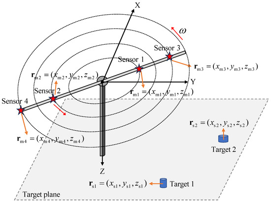
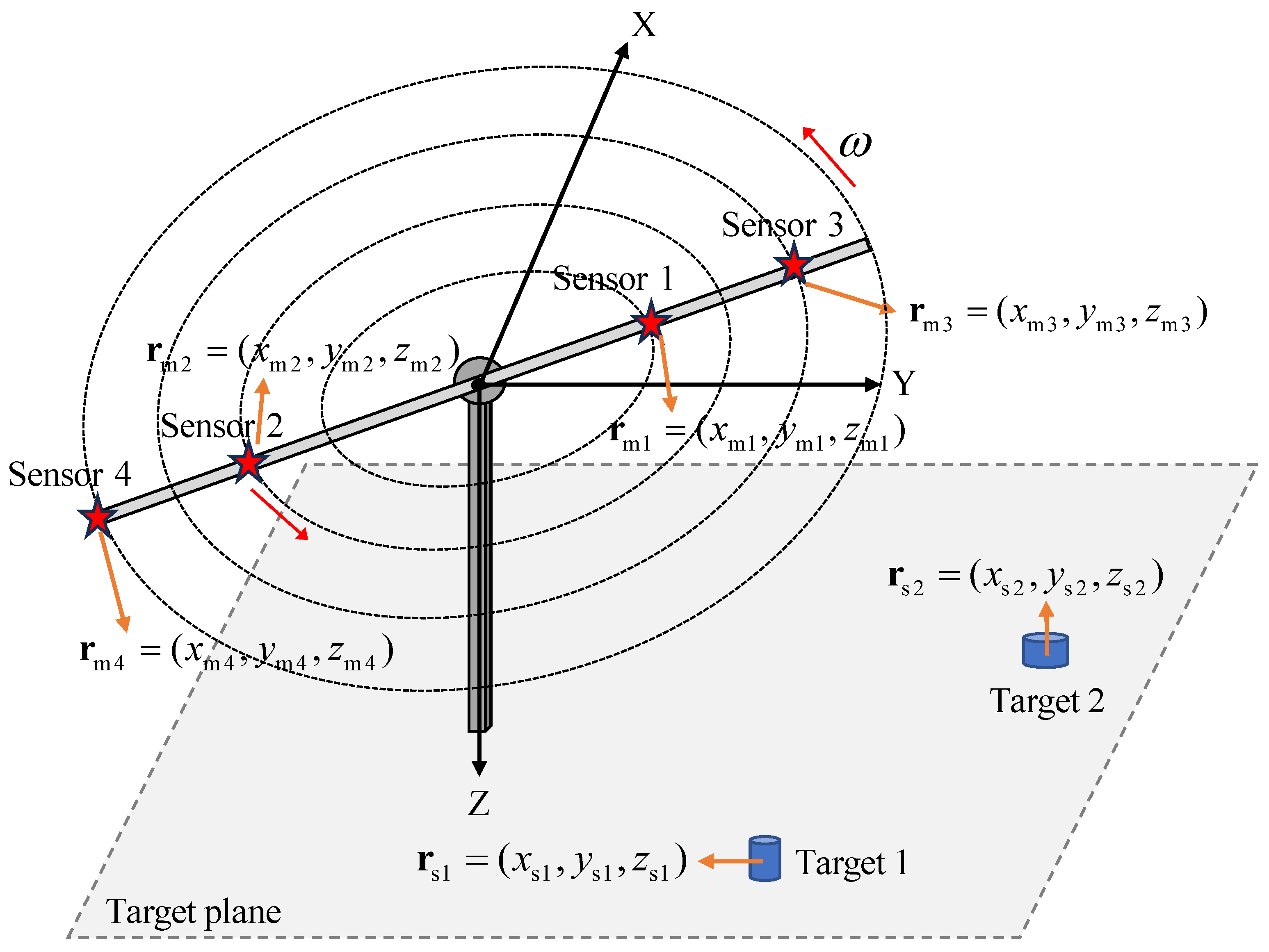
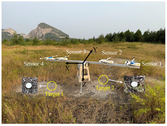
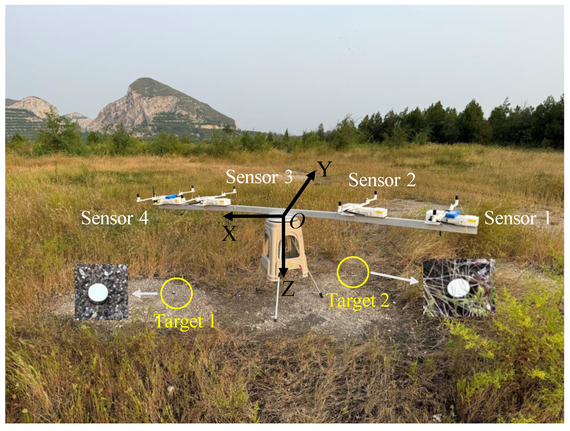
Our measurement setting utilizes an automatic rotating track made of non-magnetic material as the sensor platform. Multiple fluxgate sensors are integrated into this platform to acquire magnetic field data through a rotating scanning approach. Figure 1 illustrates four sensors and two targets for localization. A coordinate system is established, with the center of the rotating platform as the origin. The x-axis is aligned with geographic north, the y-axis points eastward, and the z-axis is perpendicular downward. If the distance between the sensor and the target exceeds three times the target’s dimensions, the target can be regarded as a magnetic dipole [24]. Assuming that there are L sensors and Q targets to be detected, the vector magnetic anomaly signal generated by the jth target at the nth measurement point measured by the ith sensor is

$${\mathbf{B}}_{\mathrm{S}ij}^{\left(n\right)}={\displaystyle \frac{\mu }{4\pi }}\left[{\displaystyle \frac{3{\mathbf{R}}_{ij}^{\left(n\right)}({\mathbf{R}}_{ij}^{\left(n\right)}·{\mathbf{M}}_j)}{{\left|{\mathbf{R}}_{ij}^{\left(n\right)}\right|}^5}}-{\displaystyle \frac{{\mathbf{M}}_j}{{\left|{\mathbf{R}}_{ij}^{\left(n\right)}\right|}^3}}\right]=\overline{\overline{\mathbf{F}}}\left({\mathbf{R}}_{ij}^{\left(n\right)}\right)·{\mathbf{M}}_j$$

(1)

$$\overline{\overline{\mathbf{F}}}\left({\mathbf{R}}_{ij}^{\left(n\right)}\right)={\displaystyle \frac{\mu }{4\pi }}{\displaystyle \frac{3{\mathbf{R}}_{ij}^{\left(n\right)}{\mathbf{R}}_{ij}^{\left(n\right)}-{\left|{\mathbf{R}}_{ij}^{\left(n\right)}\right|}^2\mathbf{I}}{{\left|{\mathbf{R}}_{ij}^{\left(n\right)}\right|}^5}},$$

(2)

where $\mu =4\pi \times {10}^{-7}$ H/m is the vacuum permeability, ${\mathbf{M}}_j$ is the jth target magnetic moment, ${\mathbf{R}}_{ij}^{\left(n\right)}={\mathbf{r}}_{\mathrm{m}i}^{\left(n\right)}-{\mathbf{r}}_{\mathrm{s}j}$ is the distance vector between jth target and ith sensor at the nth measurement point, ${\mathbf{r}}_{\mathrm{m}i}^{\left(n\right)}$ is the nth measurement point coordinate of the ith sensor provided by the GPS module, ${\mathbf{r}}_{\mathrm{s}j}$ is the jth unknown target coordinate to be solved, and $\mathbf{I}$ is the unit dyad.

Figure 1. Schematic of four magnetic sensors used for ferromagnetic target detection.

The scalar magnetic field generated by the magnetic anomaly target can be defined as the projection of the vector magnetic field onto the direction of the geomagnetic field, expressed as follows:

$$B_{\mathrm{S}ij}^{\left(n\right)}=\left|\mathbf{T}+{\mathbf{B}}_{\mathrm{S}ij}^{\left(n\right)}\right|-\left|\mathbf{T}\right|\approx \widehat{\mathbf{T}}·{\mathbf{B}}_{\mathrm{S}ij}^{\left(n\right)},(i=1,\dots L,j=1,\dots Q)$$

(3)

where $\mathbf{T}$ is the local geomagnetic field and $\widehat{\mathbf{T}}$ is its directional vector with respect to the platform measured by the sensor.

The magnetic anomaly signal sequence measured by L sensors at the nth measurement point can be expressed as follows:

$${\mathit{B}}_{\mathrm{S}}^{\left(n\right)}=\left[\begin{array}{c}{B}_{\mathrm{S}1}^{\left(n\right)}\\ ⋮\\ B_{\mathrm{S}L}^{\left(n\right)}\end{array}\right]={\overline{\overline{\mathbf{F}}}}_{\mathrm{S}}({\mathbf{r}}_{\mathrm{m}}^{\left(n\right)},{\mathbf{r}}_{\mathrm{s}})·{\mathit{M}}_{\mathrm{S}}$$

(4)

$${\overline{\overline{\mathbf{F}}}}_{\mathrm{S}}({\mathbf{r}}_{\mathrm{m}}^{\left(n\right)},{\mathbf{r}}_{\mathrm{s}})={\overline{\overline{\mathbf{T}}}}_{\mathrm{all}}·\left[\begin{array}{ccc}\overline{\overline{\mathbf{F}}}({\mathbf{r}}_{\mathrm{m}1}^{\left(n\right)},{\mathbf{r}}_{\mathrm{s}1})& \dots & \overline{\overline{\mathbf{F}}}({\mathbf{r}}_{\mathrm{m}1}^{\left(n\right)},{\mathbf{r}}_{\mathrm{s}Q})\\ ⋮& & ⋮\\ \overline{\overline{\mathbf{F}}}({\mathbf{r}}_{\mathrm{m}L}^{\left(n\right)},{\mathbf{r}}_{\mathrm{s}1})& \dots & \overline{\overline{\mathbf{F}}}({\mathbf{r}}_{\mathrm{m}L}^{\left(n\right)},{\mathbf{r}}_{\mathrm{s}Q})\end{array}\right]$$

(5)

$${\mathit{M}}_{\mathrm{S}}={[{\mathbf{M}}_1,\dots ,{\mathbf{M}}_Q]}^{\mathrm{T}}$$

(6)

where $B_{\mathrm{S}i}^{\left(n\right)}={\sum }_{j=1}^Q{B}_{\mathrm{S}ij}^{\left(n\right)}$$(i=1,\dots L)$ is the sum of the magnetic anomaly signals generated by all targets measured by the ith sensor and ${\overline{\overline{\mathbf{T}}}}_{\mathrm{all}}$ is an L × 3L block diagonal matrix, where each diagonal block is the 1 × 3 vector $\widehat{\mathbf{T}}$.

In real-world environments, the total magnetic field measured by sensors at the nth measurement point includes not only magnetic anomaly signals ${\mathit{B}}_{\mathrm{S}}^{\left(n\right)}$ but also the local geomagnetic field $\mathit{T}$ and other magnetic noise ${\mathit{B}}_{\mathrm{noi}}^{\left(n\right)}$. Therefore, the total magnetic field sequence containing all measurement points can be expressed as

$${\mathit{B}}_{\mathrm{total}}={\mathit{B}}_{\mathrm{S}}+\mathit{T}+{\mathit{B}}_{\mathrm{noi}}.$$

(7)

To reduce the number of parameters to be estimated and improve the accuracy of target position estimation, we employ an odd/even separation method to eliminate the influence of the target’s magnetic moment and the geomagnetic field. Based on parity of the sampling point indices, ${\mathit{B}}_{\mathrm{total}}$ is divided into two subsets: the magnetic field measured at odd-indexed points is denoted as ${\mathit{B}}_{\mathrm{odd}}$, while that measured at even-indexed points is denoted as ${\mathit{B}}_{\mathrm{even}}$:

$${\mathit{B}}_{\mathrm{odd}}={\overline{\overline{\mathbf{F}}}}_{\mathrm{S}}({\mathbf{r}}_{\mathrm{m}\mathrm{o}},{\mathbf{r}}_{\mathrm{s}})·{\mathit{M}}_{\mathrm{S}}+\mathit{T}+{\mathit{B}}_{\mathrm{noi}\_\mathrm{o}}$$

(8)

$${\mathit{B}}_{\mathrm{even}}={\overline{\overline{\mathbf{F}}}}_{\mathrm{S}}({\mathbf{r}}_{\mathrm{m}\mathrm{e}},{\mathbf{r}}_{\mathrm{s}})·{\mathit{M}}_{\mathrm{S}}+\mathit{T}+{\mathit{B}}_{\mathrm{noi}\_\mathrm{e}}$$

(9)

where ${\mathbf{r}}_{\mathrm{mo}}$ is the coordinate sequence corresponding to the odd measurement points and ${\mathbf{r}}_{\mathrm{me}}$ corresponds to the even measurement points. To make the anomaly signal and geomagnetic field comparable in magnitude, we intentionally introduce a reference value $B_{\mathrm{ref}}=\mathrm{50,000}$ nT with $\mathit{T}=(B_{\mathrm{ref}}+\mathsf{\Delta }T)\mathit{E}$, where $\mathit{E}$ is a unit column vector; thus, (8) can be written as

$$\begin{array}{cc}\hfill {\mathit{B}}_{\mathrm{odd}}-B_{\mathrm{ref}}\mathit{E}& ={\overline{\overline{\mathbf{F}}}}_{\mathrm{S}}({\mathbf{r}}_{\mathrm{m}\mathrm{o}},{\mathbf{r}}_{\mathrm{s}})·{\mathit{M}}_{\mathrm{S}}+\mathsf{\Delta }T\mathit{E}+{\mathit{B}}_{\mathrm{noi}\_\mathrm{o}},\hfill \end{array}$$

(10)

$$\begin{array}{cc}\hfill \mathsf{\Delta }{\mathit{B}}_{\mathrm{odd}}& ={\overline{\overline{\mathbf{F}}}}_{\mathrm{total}}({\mathbf{r}}_{\mathrm{m}\mathrm{o}},{\mathbf{r}}_{\mathrm{s}})·\left[\begin{array}{c}{\mathit{M}}_{\mathrm{S}}\\ \mathsf{\Delta }T\end{array}\right]+{\mathit{B}}_{\mathrm{noi}\_\mathrm{o}},\hfill \end{array}$$

(11)

where ${\overline{\overline{\mathbf{F}}}}_{\mathrm{total}}({\mathbf{r}}_{\mathrm{m}\mathrm{o}},{\mathbf{r}}_{\mathrm{s}})=\left[\begin{array}{cc}{\overline{\overline{\mathbf{F}}}}_{\mathrm{S}}({\mathbf{r}}_{\mathrm{m}\mathrm{o}},{\mathbf{r}}_{\mathrm{s}})& \mathit{E}\end{array}\right]$. Similarly,

$$\mathsf{\Delta }{\mathit{B}}_{\mathrm{even}}={\overline{\overline{\mathbf{F}}}}_{\mathrm{total}}({\mathbf{r}}_{\mathrm{m}\mathrm{e}},{\mathbf{r}}_{\mathrm{s}})·\left[\begin{array}{c}{\mathit{M}}_{\mathrm{S}}\\ \mathsf{\Delta }T\end{array}\right]+{\mathit{B}}_{\mathrm{noi}\_\mathrm{e}}.$$

(12)

From (11), we get

$$\left[\begin{array}{c}{\mathit{M}}_{\mathrm{S}}\\ \mathsf{\Delta }T\end{array}\right]\approx {\left[{\overline{\overline{\mathbf{F}}}}_{\mathrm{total}}{({\mathbf{r}}_{\mathrm{mo}},{\mathbf{r}}_{\mathrm{s}})}^{\mathrm{T}}·{\overline{\overline{\mathbf{F}}}}_{\mathrm{total}}({\mathbf{r}}_{\mathrm{mo}},{\mathbf{r}}_{\mathrm{s}})\right]}^{-1}·\left[{\overline{\overline{\mathbf{F}}}}_{\mathrm{total}}{({\mathbf{r}}_{\mathrm{mo}},{\mathbf{r}}_{\mathrm{s}})}^{\mathrm{T}}·\mathsf{\Delta }{\mathit{B}}_{\mathrm{odd}}\right].$$

(13)

Then, substituting (13) into (12), we obtain an expression that only contains the target coordinates:

$$\mathsf{\Delta }{\mathit{B}}_{\mathrm{even}}\approx \overline{\overline{\mathbf{G}}}·\mathsf{\Delta }{\mathit{B}}_{\mathrm{odd}}$$

(14)

$$\overline{\overline{\mathbf{G}}}={\overline{\overline{\mathbf{F}}}}_{\mathrm{total}}({\mathbf{r}}_{\mathrm{m}\mathrm{e}},{\mathbf{r}}_{\mathrm{s}})·{\left[{\overline{\overline{\mathbf{F}}}}_{\mathrm{total}}{({\mathbf{r}}_{\mathrm{m}\mathrm{o}},{\mathbf{r}}_{\mathrm{s}})}^{\mathrm{T}}·{\overline{\overline{\mathbf{F}}}}_{\mathrm{total}}({\mathbf{r}}_{\mathrm{m}\mathrm{o}},{\mathbf{r}}_{\mathrm{s}})\right]}^{-1}·{\overline{\overline{\mathbf{F}}}}_{\mathrm{total}}{({\mathbf{r}}_{\mathrm{m}\mathrm{o}},{\mathbf{r}}_{\mathrm{s}})}^{\mathrm{T}}$$

(15)

2.2. QPSO-GA Joint Algorithm

The magnetic target localization problem exhibits characteristics such as multiple local minima and susceptibility to noise interference. To solve the target’s coordinates, we propose a joint QPSO-GA algorithm that integrates the strengths of quantum-behavior particle swarm optimization (QPSO) [25,26] and a genetic algorithm (GA) [27,28]. In the proposed joint strategy, QPSO is first employed to achieve rapid convergence and local optimization. Subsequently, genetic operators (selection, crossover, and mutation) from GAs are introduced to reorganize and optimize the particle swarm. This operation helps the algorithm escape local optima, further ensuring that the more precise global optimum solution is obtained. Additionally, the population diversity mechanism of the GA effectively prevents the joint algorithm from over-reliance on a single search path, while the quantum characteristics of QPSO significantly reduce dependence on initial population settings. The combination of both ensures that the algorithm maintains strong robustness in magnetic field environments contaminated by noise. A detailed description of this algorithm is provided below.

(1) Fitness Function: In optimization problems, it is necessary to construct a fitness function to evaluate the quality of solutions. According to Equation (15), the residual vector $\mathit{e}$ is defined as the difference between the actual value $\mathsf{\Delta }{\mathit{B}}_{\mathrm{even}}$ and the predicted value $\overline{\overline{\mathbf{G}}}·\mathsf{\Delta }{\mathit{B}}_{\mathrm{odd}}$. This residual is used to quantify the prediction error, thereby guiding the optimization process. The optimization algorithm uses the standard deviation (STD) of $\mathit{e}$ as the fitness function, and its expression is as follows:

$$\mathrm{Fit}=\sqrt{{\displaystyle \frac{1}{N-1}}\Vert \mathsf{\Delta }{\mathit{B}}_{\mathrm{even}}-\overline{\overline{\mathbf{G}}}·\mathsf{\Delta }{\mathit{B}}_{\mathrm{odd}}{\Vert }_2^2}$$

(16)

where N is the total number of measurement points in the odd/even sequence. We need to search for the target’s coordinates ${\mathbf{r}}_{\mathrm{s}}$ within the specified range to minimize the fitness value.

(2) Algorithm Update Strategy: During the iterative process of the joint algorithm, the implementation steps are as follows. In each iteration, particle positions are first updated using the quantum leap operation from QPSO to enable efficient optimization, as described in (17)–(22). Subsequently, genetic operations from the GA (including selection, crossover, and mutation) are introduced to reorganize and perturb the population, as specified in (23)–(25). Let $N_{\mathrm{p}}$ denote the number of particles, $N_{\mathrm{ger}}$ the maximum number of iterations, and D the dimensionality of the problem (in this paper, $D=3$); the variables $ub$ and $lb$ represent the upper and lower bounds of the search range, respectively, the position of the ith particle in the kth generation is denoted as ${\mathbf{x}}_i^k\in {\mathbb{R}}^D$, and the individual best position ($p_{best}$) is denoted as ${\mathbf{p}}_i^k$, while the population best ($g_{best}$) is ${\mathbf{g}}^k$.

First, we employ the parameter update strategy of QPSO. The particle positions are updated by

$${\mathbf{x}}_i^{k+1}={\mathbf{x}}_i^k+{\mathbf{v}}_i^{k+1},$$

(17)

$${\mathbf{v}}_i^{k+1}=w_t{\mathbf{v}}_i^k+c_p{\mathbf{b}}_1·({\mathbf{p}}_i^k-{\mathbf{x}}_i^k)+c_g{\mathbf{b}}_2·({\mathbf{g}}^k-{\mathbf{x}}_i^k),$$

(18)

where ${\mathbf{v}}_i^k\in {\mathbb{R}}^D$ is the velocity of the ith particle at the kth generation, ${\mathbf{b}}_1,{\mathbf{b}}_2\in {[0,1]}^D$ are random vectors, $c_p$ and $c_g$ are the individual learning factor and group learning factor, respectively, and $w_t$ is a constant linear descent used to balance global or local search:

$$w_t=w_{max}-(w_{max}-w_{min})·{\displaystyle \frac{k}{N_{\mathrm{ger}}}}.$$

(19)

The particle potential well-center attractor is then calculated:

$${\mathbf{P}}_i^k=\varphi {\mathbf{p}}_i^k+(1-\varphi ){\mathbf{g}}^k,\varphi \in (0,1).$$

(20)

Quantum leap operation further updates the location parameters:

$${\mathrm{mbest}}^k={\displaystyle \frac{1}{N_p}}\sum _{j=1}^{N_p}{\mathbf{p}}_j^k,$$

(21)

$${\mathbf{x}}_i^{k+1}={\mathbf{P}}_i^k\pm {\alpha }_k|{\mathrm{mbest}}^k-{\mathbf{x}}_i^k|·ln\left(1./\mathbf{u}\right),$$

(22)

where $\mathbf{u}\in {(0,1)}^D$. Here, ${\alpha }_k$ has an initial value of 1 and decays generation-by-generation.

Subsequently, the elite crossover and mutation operations of the GA are employed to enhance diversity; $N_e$ elite individuals are selected and ranked according to the fitness values of their personal best positions ($p_{best}$). These undergo arithmetic crossover operations in randomly assigned pairs:

$${\mathrm{child}}_1=\beta ·{\mathbf{p}}_a+(1-\beta )·{\mathbf{p}}_b,$$

(23)

$${\mathrm{child}}_2=\beta ·{\mathbf{p}}_b+(1-\beta )·{\mathbf{p}}_a,$$

(24)

where $\beta \in {[0,1]}^D$ is a randomly generated weighting vector and where ${\mathbf{p}}_a$ and ${\mathbf{p}}_b$ represent two parent generations. Gaussian perturbation is then applied to each dimension of the offspring with mutation probability $p_{\mathrm{mut}}$:

$$\mathrm{child}\leftarrow \mathrm{child}+\mathcal{N}\left(0,{(\sigma ·(ub-lb))}^2\right)$$

(25)

where $\sigma$ is the standard deviation of the mutation. The newly generated offspring then replace the worst-performing individuals in the current population ${\mathbf{x}}_i^{k+1}$, thereby preserving high-quality solutions while enhancing diversity.

The pseudocode for the joint algorithm is shown in the Algorithm 1. In this study, the dimension D is 3, the number of particles $N_p$ is 500, the number of iterations $N_{\mathrm{ger}}$ is 30, $w_{max}$ is 0.9, $w_{min}$ is 0.4, $c_p$ and $c_g$ are both 0.5, $p_{\mathrm{mut}}$ is 0.15, and $\sigma$ is 0.05. These key hyperparameters were obtained through a series of experiments. First, reasonable boundary values were set for each hyperparameter based on the existing literature. Subsequently, Bayesian optimization was employed to search for and obtain the optimal key hyperparameters. Finally, evaluation was conducted on the test set.

3. Experiment Validation

3.1. Simulation Experiments

To verify the effectiveness of the proposed method, we conducted some numerical experiments. In the simulation experiments, the rotational measurement plane is defined at $z=0$, with the z-axis oriented vertically downward. Each experiment generated four full rotation cycles, with 200 measurement points per cycle. The magnetic anomaly signal is simulated using (4), with Gaussian white noise added at a specified signal-to-noise ratio (SNR). The SNR is defined as $\mathrm{SNR}=20\ast \log 10(\mathrm{S}/\mathrm{N})$ dB, where S and N are the peak-to-peak values of the signal and noise. The inclination and declination angles of the target vary uniformly within the ranges $[0°,180°]$ and $[0°,360°]$, respectively, while the magnetic moment magnitude ranges from 5 to 15 A·m². The detection region is bounded by $x\in [-2,2]$ m, $y\in [-2,2]$ m, and $z\in [0,2]$ m. The set of target coordinates is randomly and uniformly distributed within this area.

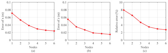
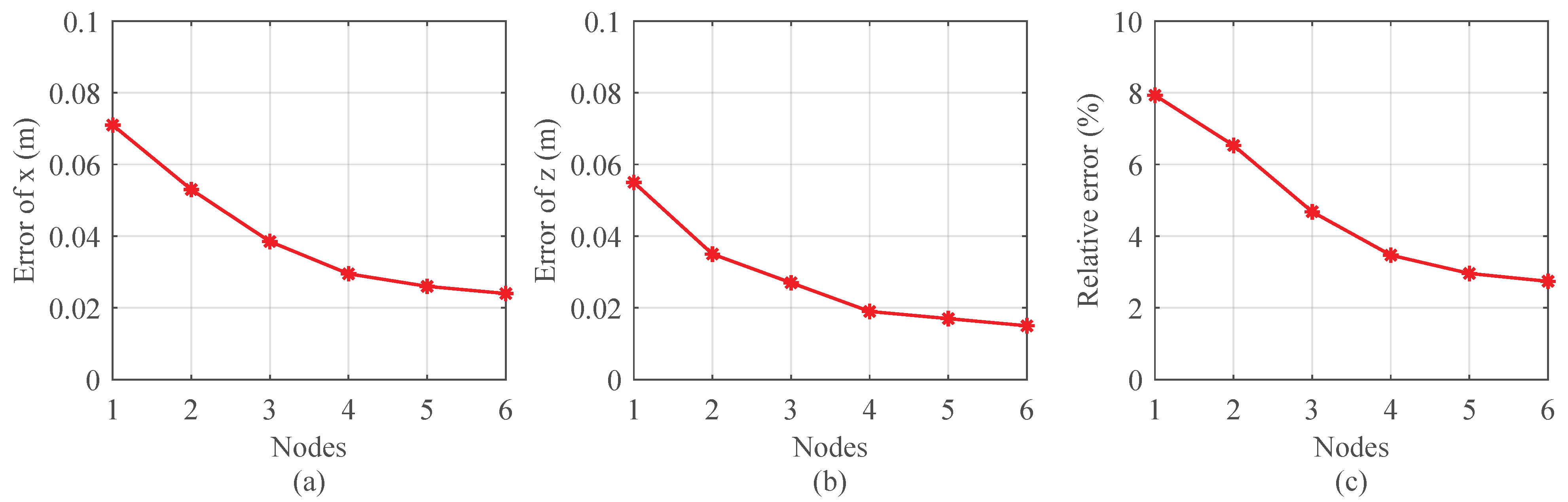
To evaluate the impact of the number of sensor nodes on the localization accuracy of a single target, a series of Monte Carlo simulations were conducted at SNR of 5 dB, as shown in Figure 2. In the experiment, sensors were uniformly distributed along radial lines extending from the rotation center within a 4 m × 4 m area. Figure 2a,b presents the positioning errors averaged over 1000 trials in the x-direction and z-direction, respectively. Because the error distribution in the y-direction was similar to that in the x-direction, the y-direction error is not displayed. Figure 2c shows the relative magnetic moment error calculated by inversion based on the positioning results. The results indicate that as the number of sensor nodes increases, both the localization error and the magnetic moment error gradually decrease. We tested the runtime with varying numbers of sensors. The positioning time results using one, two, three, and four sensors are 15.693 s, 24.312 s, 35.569 s, and 48.902 s respectively, all within an acceptable range. With four sensor nodes, the average positioning errors in the x-direction and z-direction are 0.03 m and 0.02 m, respectively, and a relative magnetic moment error of 3.47%. The errors decrease rapidly before the number of nodes reaches four, after which the error decreases slowly. Therefore, in a 4 m × 4 m area, using four nodes for localizing the target is most appropriate.

Figure 2. Average errors with different quantities of sensor nodes for single-target positioning in a 4 m × 4 m survey area: (a) localization errors in the x-direction, (b) localization errors in the z-direction, and (c) relative errors of the estimated target magnetic moment.

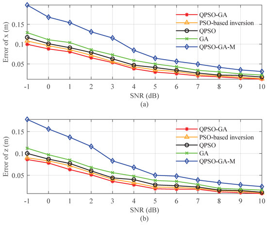
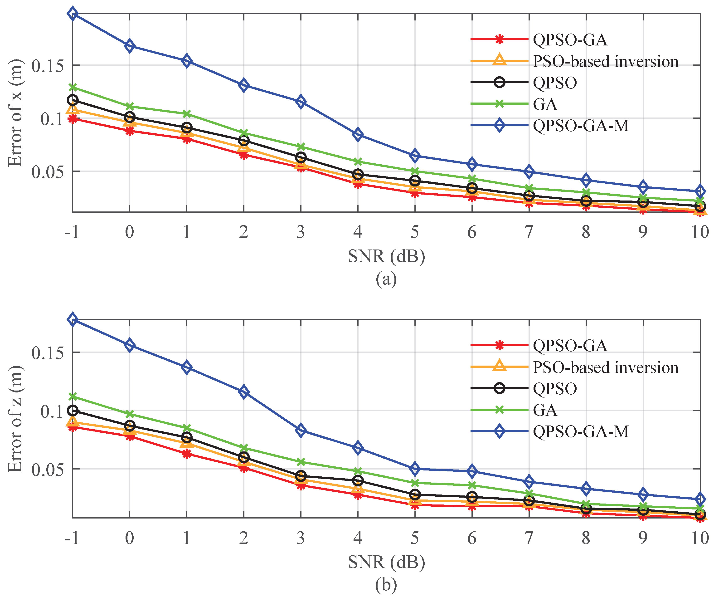
Figure 3, shows the results of 1000 Monte Carlo simulations performed at each SNR to compare the performance of our algorithm with other algorithms.

Figure 3. Average errors of different algorithms for single-target positioning using four sensors at varying SNRs in a 4 m × 4 m survey area. (a) Localization errors in the x-direction. (b) Localization errors in the z-direction.

The algorithms used for comparison are: the gradient parameters inversion algorithm based on particle swarm optimization (PSO) [19]; quantum particle swarm optimization (QPSO) and the genetic algorithm (GA), both of which estimate target coordinates with the proposed fitness function; and a variant of the QPSO-GA algorithm that simultaneously estimates both the magnetic moments and target coordinates without eliminating the magnetic moments, denoted as QPSO-GA-M. In this setup, four sensors are used to detect a single target, respectively positioned at distances of 0.5 m, 1 m, 1.5 m, and 2 m from the center of rotation; the average positioning errors in the x-direction and z-direction are shown in Figure 3a,b. Experimental results show that the proposed algorithm achieves smaller estimation errors compared to the latest PSO-based inversion algorithm, particularly at low SNRs. Compared to the QPSO-GA-M algorithm, the proposed method significantly reduces errors, demonstrating the benefit of reducing the number of unknowns by eliminating the magnetic moment. Furthermore, the proposed algorithm consistently outperforms both QPSO and GA algorithms across all SNR levels, confirming its effective integration of the strengths of both QPSO and GA to achieve higher estimation accuracy and stronger robustness.

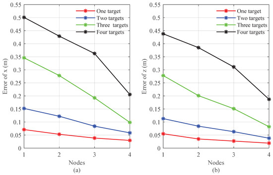
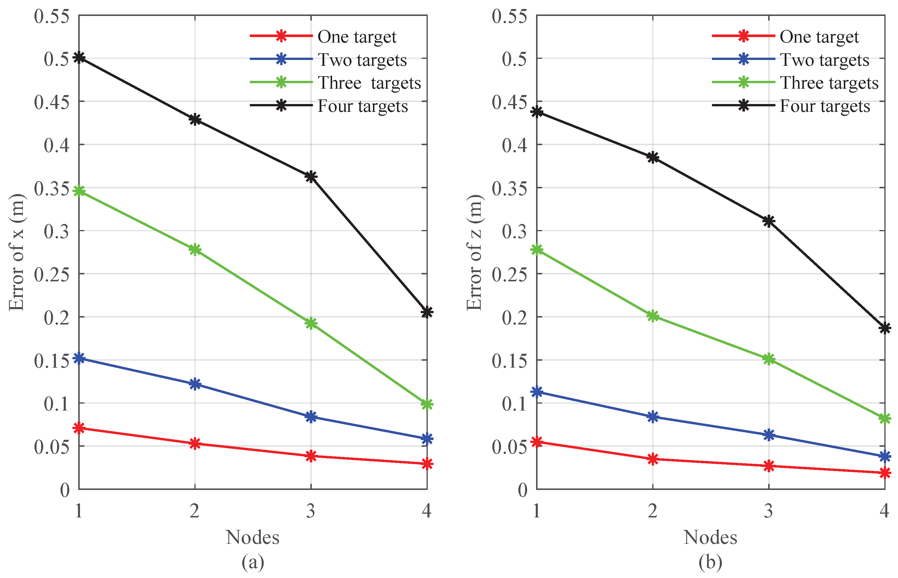
In multi-target localization tasks, the number of sensors and targets are both critical factors influencing localization accuracy. To systematically investigate the relationship between these factors, we designed the simulation experiment shown in Figure 4. This experiment includes multiple configuration schemes, such as one sensor detecting one to four targets, two sensors detecting one to four targets, and so forth. For each sensor–target configuration, 1000 Monte Carlo experiments were conducted. Figure 4a,b presents the average localization errors in the x- and z-directions, respectively. The results indicate that when the number of sensors is fixed, the localization error increases with the number of targets; conversely, when the number of targets is fixed, the error decreases as the number of sensors increases. Overall, higher localization accuracy is achieved when the number of sensors exceeds the number of targets. To ensure optimal performance, it is recommended to use at least two more sensors than the number of targets. We also analyzed the computational costs. When using four sensors to locate one, two, and three targets the required times were 48.902 s, 70.843 s, and 102.176 s, respectively. Our measurement method is similar to the point-by-point measurement. The time allocated for each relocation and measurement is fully reserved for processing the data acquired from the previous set.

Figure 4. Average localization errors using the proposed algorithm for varying numbers of sensor nodes and targets in a 4 m × 4 m area: (a) localization errors in the x-direction and (b) localization errors in the z-direction.

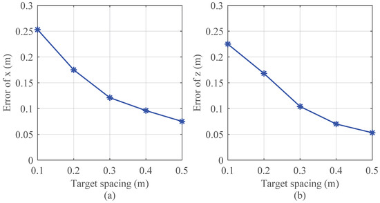
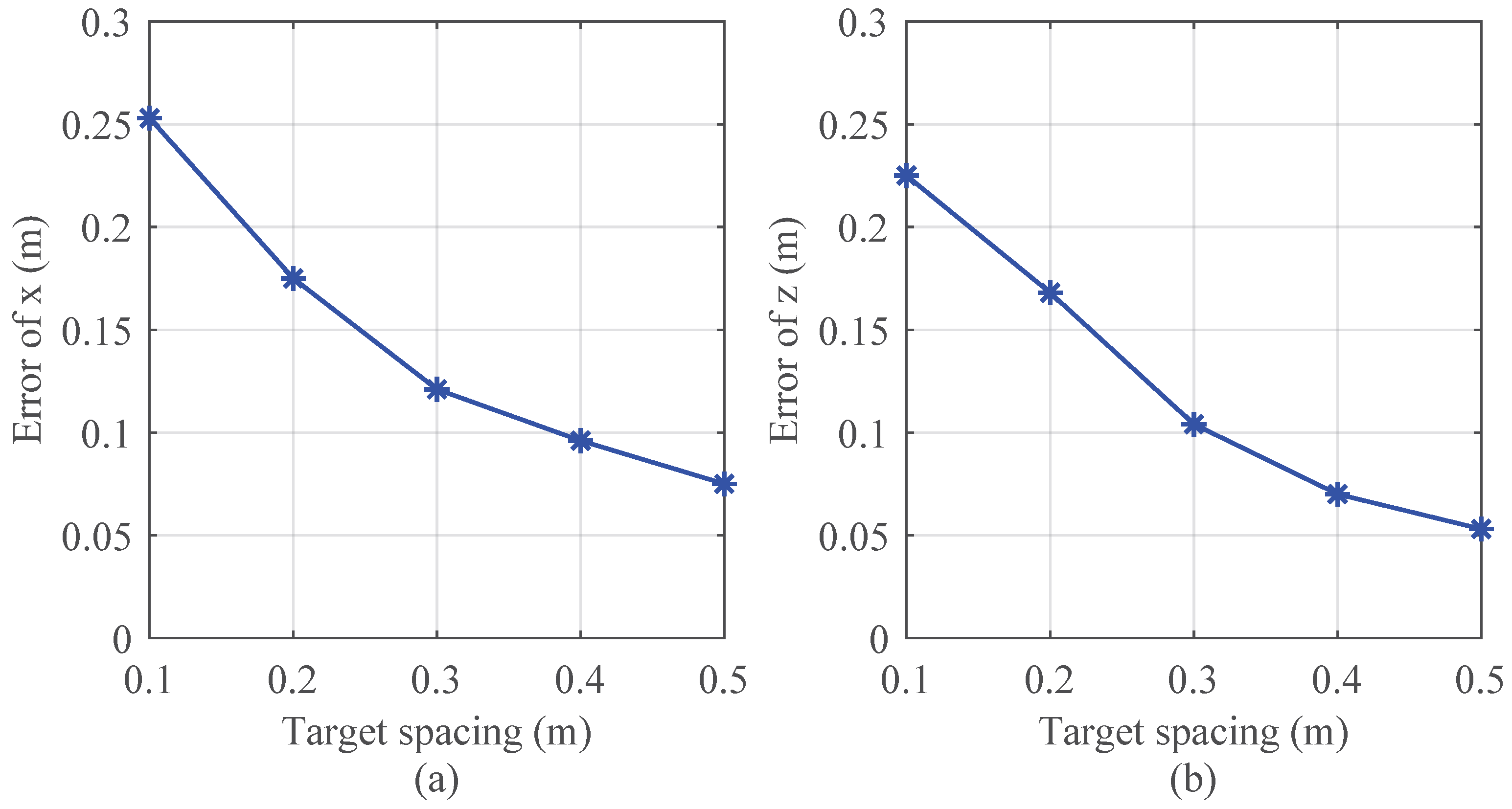
To investigate the impact of target spacing on positioning accuracy in multi-target localization, we carried out a series of simulation experiments. The experiments employed four sensors to detect two targets, evaluating positioning performance by adjusting the spacing between targets (ranging from 0.1 m to 0.5 m). We calculated the average positioning error to quantify the effect of spacing variation on accuracy. As shown in the Figure 5, the positioning error increases as the target spacing decreases. This is because when targets are too close, their magnetic fields overlap and interfere with each other, potentially causing nonlinear amplification or cancellation that degrades positioning accuracy. We also conducted a simulation experiment using four sensors to detect four targets. Two of the targets were placed relatively close together, with a spacing of 0.3 m, while the other two targets were placed farther apart. Fifty trials were performed in total. The results indicate that the average positioning error for the two closely spaced targets is 0.314 m in the x-direction and 0.291 m in the z-direction. For the two more distant targets, the average positioning errors are 0.223 m in the x-direction and 0.206 m in the z-direction. The positioning error for the distant target aligns with the simulation results in Figure 4, while the positioning error for the closer target is increased.

Figure 5. Average localization errors using the proposed algorithm for varying target spacing in a 4 m × 4 m area: (a) localization errors in the x-direction and (b) localization errors in the z-direction.

3.2. Field Experiments

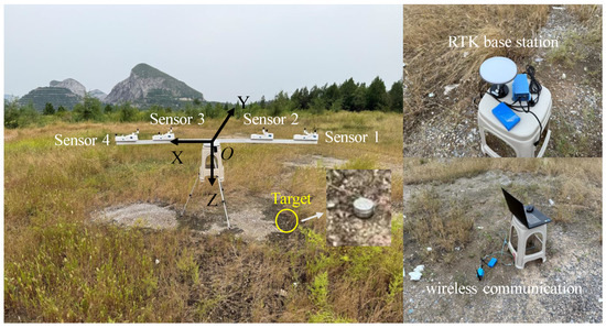
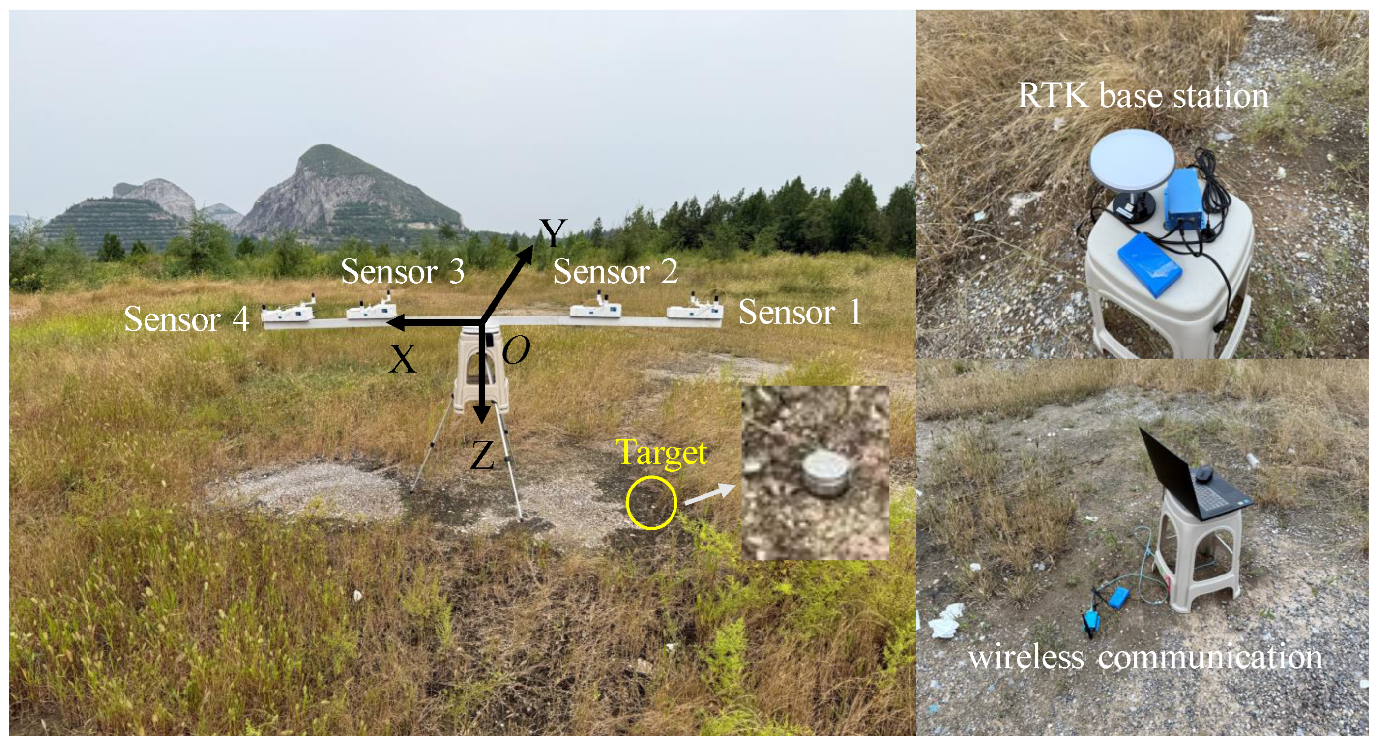
A field experiment was carried out in the suburbs of Beijing. The location is shown in Figure 6, and was selected for its minimal environmental electromagnetic interference. The measurement platform consisted of four core components: an automatically rotating non-magnetic track, four Bartington Mag649FLL fluxgate sensors, a real-time kinematic (RTK) base station, and a wireless communication module. The sensors were mounted on the track to collect three-axis magnetic field data, attitude angles, and GPS positioning information. The RTK base station provided reference coordinates with millimeter-level accuracy, and positioning errors from the sensors had minimal impact on target positioning precision. The wireless communication module facilitated data transmission and command distribution between the host computer and the sensors. During rotation, the magnetic field data and GPS information collected by the sensors at different positions were transmitted in real-time to the host computer, ensuring data synchronization and integrity.

Figure 6. Scene photograph of the field experiment for localizing a single target.

First, we performed an experiment for localizing a single target. The experimental setup is illustrated in Figure 6. The target was a circular iron block with a diameter of approximately 5 cm, placed directly on a flat ground surface for ease of placement and positioning. A coordinate system was established with the rotation center as the origin O, the x-axis aligned with geographic north, the y-axis pointing east, and the z-axis is perpendicular downward, with the rotational measurement plane corresponding to $z=0$. The measurement area was set to $x\in [-2,2]$ m, $y\in [-2,2]$ m, and $z\in [0,2]$ m. The target was located at coordinates (−1.1, 0, 0.85) m. The true coordinates of the target were derived from the latitude and longitude measurements collected by the high-precision real-time kinematic (RTK) GPS system as raw data and converted using proven formulas [29], achieving a reference position with millimeter-level accuracy. Magnetic field data were collected through six rotations to support subsequent localization analysis.

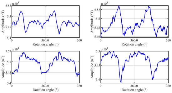
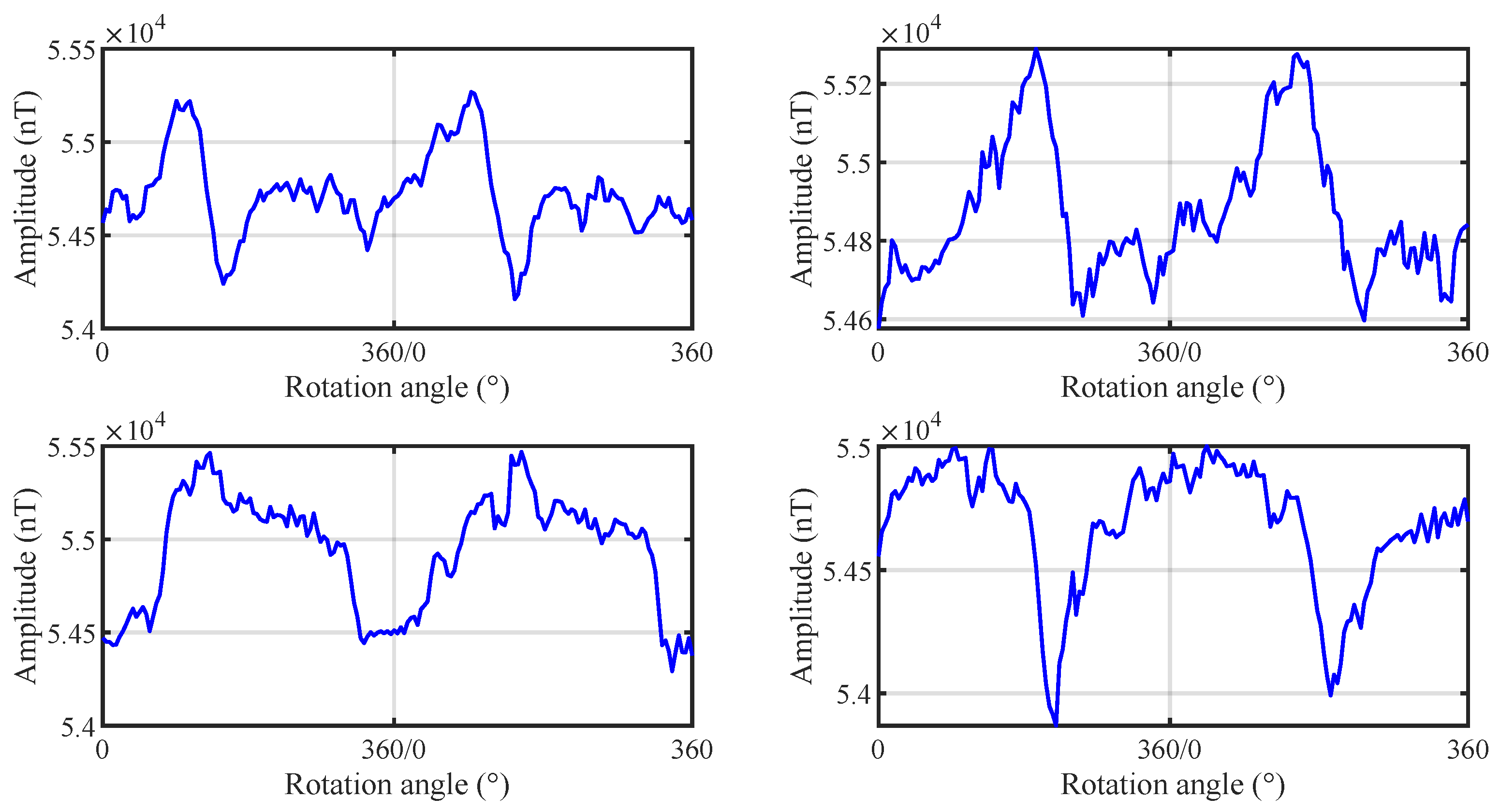
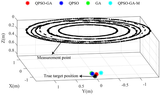
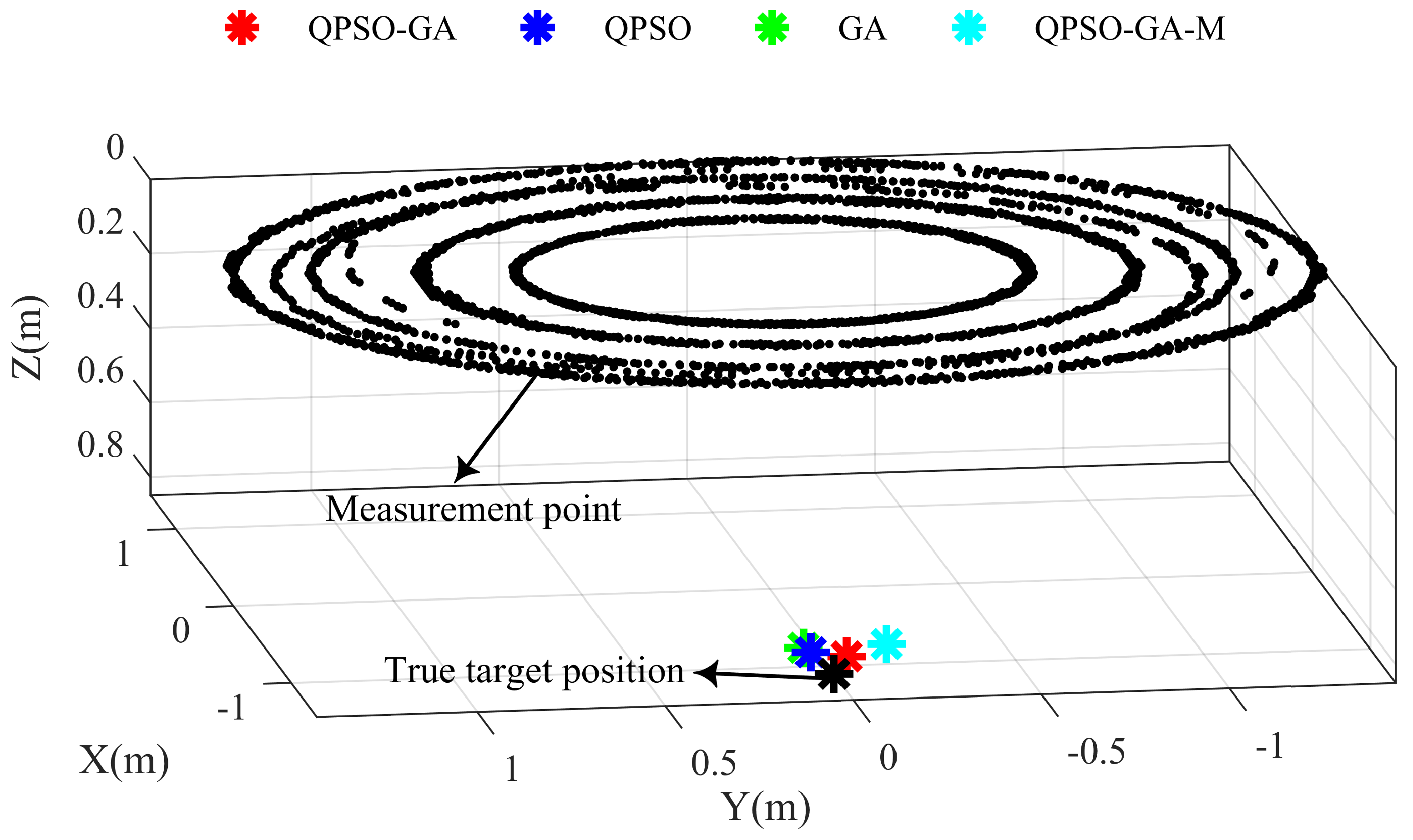
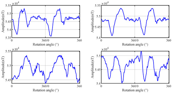
Figure 7 shows a segment of the total magnetic field measured by four sensor nodes in the single-target localization experiment, containing two complete cycles; the measured magnetic field exhibits distinct periodic variations with relatively clear anomaly signals. Figure 8 illustrates the estimated target positions obtained by different algorithms. It can be observed that the coordinates estimated by the proposed algorithm are closest to the true target position compared to other algorithms. The corresponding localization errors are summarized in Table 1. Our algorithm achieves localization errors of less than 0.06 m in the x-, y-, and z-directions, outperforming the other compared algorithms and highlighting the effectiveness and advantages of the joint algorithm in real-world detection. Furthermore, the target magnetic moment obtained through inversion is 10.519 A·m², and its relative error can be evaluated with reference to the error statistics of magnetic moment estimation from the simulation experiments. We also analyzed the computational complexity for locating a single real target. The results indicate that the proposed algorithm requires 50.743 s of runtime and converges to a stable state after 25 iterations.

Figure 7. The real total magnetic fields measured by four sensor nodes in the single-target localization experiment.

Figure 8. Localization results by different algorithms for a single target in the real-world field experiment. Black points denote measurement points of sensors. The black asterisk marks the true target position, the red asterisk indicates the estimated position using the proposed QPSO-GA algorithm, the light blue asterisk shows the result of the QPSO-GA-M algorithm, and the blue and green asterisks represent estimates from the QPSO and GA algorithms, respectively.

Table 1. Positioning errors for a real target using different algorithms in a 4 m × 4 m area.

Algorithms	Position Estimation (Unit: m)			Positioning Error (Unit: m)
	x	y	z	$\mathsf{\Delta }\mathbf{x}$	$\mathsf{\Delta }\mathbf{y}$	$\mathsf{\Delta }\mathbf{z}$
QPSO-GA	−1.048	−0.043	0.815	−0.052	0.043	0.035
QPSO	−1.037	0.051	0.804	−0.063	−0.051	0.046
GA	−1.024	0.068	0.793	−0.076	−0.068	0.057
QPSO-GA-M	−1.236	−0.120	0.746	0.136	0.120	0.104

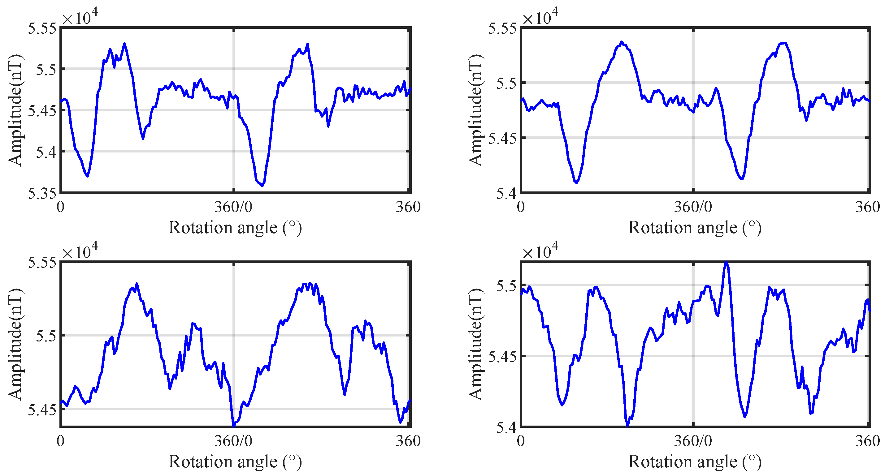
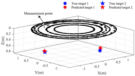
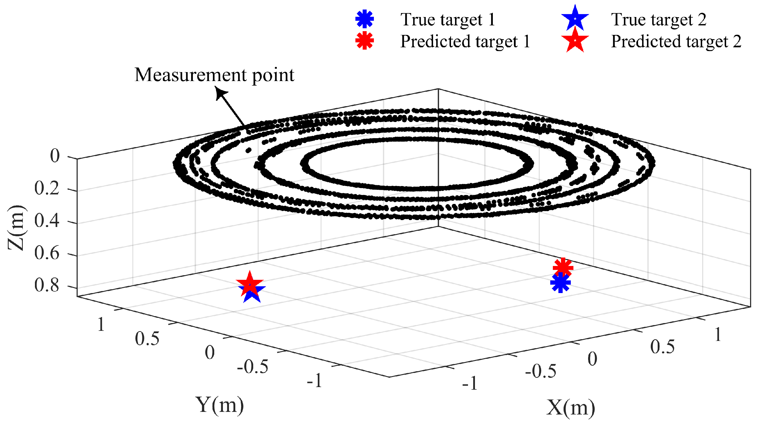
Subsequently, we carried out an experiment for localization of two targets. Figure 9 shows the experimental scene, where the coordinates of the two targets are (1.0, −0.2, 0.85) m and (−0.55, 0.85, 0.85) m, respectively. Figure 10 displays a segment of the measured total magnetic field, containing two cycles. Compared to the single-target case, the magnetic field within each cycle exhibits multiple superimposed peak characteristics. Figure 11 presents the corresponding localization results, indicating that the estimated positions are close to the true target positions. The localization errors for the two targets are summarized in Table 2. In the 4 m × 4 m measurement area, the average localization errors in the x-, y-, and z-directions are all less than 10 cm, demonstrating that the proposed algorithm can accurately estimate target positions in practical multi-target localization tasks. The error increases slightly compared to the single-target localization case, primarily due to the increased number of unknown parameters to be estimated.

Figure 9. Scene photograph of the field experiment for localizing two targets.

Figure 10. The real measured total magnetic fields by four sensor nodes in the two target localization experiment.

Figure 11. Localization results for two targets using the proposed algorithm in the real-world field experiment. Black points denote measurement points of sensors, the blue asterisk and pentagram mark the true target positions of targets, and the red asterisk and pentagram indicate the estimated positions.

Table 2. Positioning errors for two real targets using the proposed algorithm in a 4 m × 4 m area.

Targets	True Position (Unit: m)			Estimated Position (Unit: m)			Estimated Magnetic Moment
	x	y	z	x	y	z	(Unit: A·m2)
Magnet 1	1.000	−0.200	0.850	1.087	−0.121	0.785	10.687
Magnet 2	−0.550	0.850	0.850	−0.639	0.768	0.782	10.803
Average error				0.088	0.081	0.067	-

4. Concluding Remarks

This paper proposes an alternative scheme for locating buried magnetic targets based on a rotating magnetic sensor array and a joint optimization algorithm. Given the instability and inefficiency of row scanning mode on rugged terrain, we adopt a rotating scanning measurement approach. To reduce the number of unknown parameters and improve positioning accuracy, the magnetic moment and the geomagnetic field are eliminated during the modeling process. To further enhance the accuracy of target position estimation, we integrate the quantum particle swarm optimization (QPSO) algorithm with the genetic algorithm (GA), proposing a joint optimization algorithm named QPSO-GA. This algorithm combines the fast convergence and local refinement capabilities of QPSO with the global exploration and population diversity advantages of GA. Simulations and field experiments are conducted to comprehensively evaluate the localization performance of the proposed scheme. The results demonstrate that within a 4 m × 4 m measurement area, the proposed measurement setting and algorithm achieve an average localization error of less than 10 cm in multi-sensor multi-target scenarios, meeting general application requirements. Furthermore, the measurement setting can be deployed on low-magnetic unmanned platforms, making it suitable for large-scale rapid scanning and mapping tasks. For high-precision detection of small targets, replacing fluxgate sensors with optical pump magnetometers can further enhance measurement accuracy.

References

- Owen, M.; McNamara, A.; Panchal, J. The risk of unexploded ordnance on construction sites in London, UK. Environ. Geotech. 2021, 8, 116–123. [Google Scholar] [CrossRef] [Scilit]
- Taylor, S.; Bigl, S.; Packer, B. Condition of in situ unexploded ordnance. Sci. Total Environ. 2015, 505, 762–769. [Google Scholar] [CrossRef] [Scilit]
- Zhao, Y.; Zhang, J.; Li, J.; Liu, S.; Miao, P.; Shi, Y.; Zhao, E. A brief review of magnetic anomaly detection. Meas. Sci. Technol. 2021, 32, 042002. [Google Scholar] [CrossRef] [Scilit]
- Liu, H.; Zhang, X.; Dong, H.; Liu, Z.; Hu, X. Theories, applications, and expectations for magnetic anomaly detection technology: A review. IEEE Sens. J. 2023, 23, 17868–17882. [Google Scholar] [CrossRef] [Scilit]
- Chen, L.; Feng, Y.; Wu, P.; Zhu, W.; Fang, G. An innovative magnetic anomaly detection algorithm based on signal modulation. IEEE Trans. Magn. 2020, 56, 6200609. [Google Scholar] [CrossRef] [Scilit]
- Yu, J.; Li, J.; Du, C.; Peng, X.; Guo, H. An unmanned aerial vehicle magnetic detection system for archaeological exploration. Electromagn. Sci. 2025, 3, 0110122. [Google Scholar] [CrossRef] [Scilit]
- Yin, G.; Zhang, L.; Jiang, H.; Wei, Z.; Xie, Y. A closed-form formula for magnetic dipole localization by measurement of its magnetic field vector and magnetic gradient tensor. J. Magn. Magn. Mater. 2020, 499, 166274. [Google Scholar] [CrossRef] [Scilit]
- Zhi, H.; Ma, T.; Pei, D.; Sun, H. A novel magnetic dipole inversion method based on tensor geometric invariants. AIP Adv. 2020, 10, 045131. [Google Scholar] [CrossRef] [Scilit]
- Liu, G.; Zhang, Y.; Wang, C.; Li, Q.; Li, F.; Liu, W. A new magnetic target localization method based on two-point magnetic gradient tensor. Remote Sens. 2022, 14, 6088. [Google Scholar] [CrossRef] [Scilit]
- Wang, X.; Liu, H.; Wang, H.; Ge, J.; Dong, H.; Liu, Z. Quantitative analysis of the measurable areas of differential magnetic gradient tensor systems for unexploded ordnance detection. IEEE Sens. J. 2021, 21, 5952–5960. [Google Scholar] [CrossRef] [Scilit]
- Li, Q.; Li, Z.; Shi, Z.; Fan, H. Multi-target magnetic positioning using SAFCM clustering and invariants-improved tilt angle. IEEE Trans. Geosci. Remote Sens. 2022, 60, 5924015. [Google Scholar] [CrossRef] [Scilit]
- Doll, W.E.; Gamey, T.J.; Bell, D.T.; Beard, L.P.; Sheehan, J.R.; Norton, J.; Holladay, J.S.; Lee, J.L.C. Historical development and performance of airborne magnetic and electromagnetic systems for mapping and detection of unexploded ordnance. J. Environ. Eng. Geophys. 2012, 17, 1–17. [Google Scholar] [CrossRef] [Scilit]
- Du, C.; Xia, M.; Huang, S.; Xu, Z.; Peng, X.; Guo, H. Detection of a moving magnetic dipole target using multiple scalar magnetometers. IEEE Geosci. Remote Sens. Lett. 2017, 14, 1166–1170. [Google Scholar] [CrossRef] [Scilit]
- Dassot, G.; Blanpain, R.; Flament, B.; Jauffret, C. Process for Determining the Position of a Moving Object Using Magnetic Gradientmetric Measurements. U.S. Patent 6,539,327, 25 March 2003. [Google Scholar]
- Hu, S.; Tang, J.; Ren, Z.; Chen, C.; Zhou, C.; Xiao, X.; Zhao, T. Multiple underwater objects localization with magnetic gradiometry. IEEE Geosci. Remote Sens. Lett. 2019, 16, 296–300. [Google Scholar] [CrossRef] [Scilit]
- Fan, L.; Kang, X.; Zheng, Q.; Zhang, X.; Liu, X.; Chen, C.; Kang, C. A fast linear algorithm for magnetic dipole localization using total magnetic field gradient. IEEE Sens. J. 2018, 18, 1032–1038. [Google Scholar] [CrossRef] [Scilit]
- Melo, F.F.; Barbosa, V.C. Reliable Euler deconvolution estimates throughout the vertical derivatives of the total-field anomaly. Comput. Geosci. 2020, 138, 104436. [Google Scholar] [CrossRef] [Scilit]
- Davis, K.; Li, Y.; Nabighian, M. Automatic detection of UXO magnetic anomalies using extended Euler deconvolution. Geophysics 2010, 75, G13–G20. [Google Scholar] [CrossRef] [Scilit]
- Chen, Z.; Shen, Y.; Yang, X.; Gao, J.; Zhang, P.; Li, X.; Gao, Z.; Wang, X. High-Precision Depth and Magnetic Moment Inversion of Buried Unexploded Ordnance Based on Particle Swarm Optimization Algorithm. IEEE Trans. Geosci. Remote Sens. 2025, 63, 5921809. [Google Scholar] [CrossRef] [Scilit]
- Ge, J.; Wang, S.; Dong, H.; Liu, H.; Zhou, D.; Wu, S.; Luo, W.; Zhu, J.; Yuan, Z.; Zhang, H. Real-time detection of moving magnetic target using distributed scalar sensor based on hybrid algorithm of particle swarm optimization and Gauss–Newton method. IEEE Sens. J. 2020, 20, 10717–10723. [Google Scholar] [CrossRef] [Scilit]
- Alimi, R.; Geron, N.; Weiss, E.; Ram-Cohen, T. Ferromagnetic mass localization in check point configuration using a levenberg marquardt algorithm. Sensors 2009, 9, 8852–8862. [Google Scholar] [CrossRef] [Scilit]
- Alimi, R.; Weiss, E.; Ram-Cohen, T.; Geron, N.; Yogev, I. A dedicated genetic algorithm for localization of moving magnetic objects. Sensors 2015, 15, 23788–23804. [Google Scholar] [CrossRef] [Scilit]
- Sheinker, A.; Lerner, B.; Salomonski, N.; Ginzburg, B.; Frumkis, L.; Kaplan, B.Z. Localization and magnetic moment estimation of a ferromagnetic target by simulated annealing. Meas. Sci. Technol. 2007, 18, 3451. [Google Scholar] [CrossRef] [Scilit]
- Yarotskii, V.A. Optimum detection of magnetic dipoles. Meas. Tech. 1992, 35, 1190–1194. [Google Scholar] [CrossRef] [Scilit]
- Agrawal, R.; Kaur, B.; Agarwal, P. Quantum inspired particle swarm optimization with guided exploration for function optimization. Appl. Soft Comput. 2021, 102, 107122. [Google Scholar] [CrossRef] [Scilit]
- Ho, S.L.; Yang, S.; Ni, G.; Huang, J. A quantum-based particle swarm optimization algorithm applied to inverse problems. IEEE Trans. Magn. 2013, 49, 2069–2072. [Google Scholar] [CrossRef] [Scilit]
- Bansal, A.; Cannings, C.; Sheehan, N. An evaluation of the application of the genetic algorithm to the problem of ordering genetic loci on human chromosomes using radiation hybrid data. Math. Med. Biol. J. IMA 1997, 14, 161–187. [Google Scholar] [CrossRef]
- Krishna, K.; Narasimha Murty, M. Genetic K-means algorithm. IEEE Trans. Syst. Man Cybern. Part B (Cybern.) 1999, 29, 433–439. [Google Scholar] [CrossRef] [Scilit]
- Jo, K.; Lee, M.; Sunwoo, M. Fast GPS-DR Sensor Fusion Framework: Removing the Geodetic Coordinate Conversion Process. IEEE Trans. Intell. Transp. Syst. 2016, 17, 2008–2013. [Google Scholar] [CrossRef]
Disclaimer/Publisher’s Note: The statements, opinions and data contained in all publications are solely those of the individual author(s) and contributor(s) and not of MDPI and/or the editor(s). MDPI and/or the editor(s) disclaim responsibility for any injury to people or property resulting from any ideas, methods, instructions or products referred to in the content. |
© 2026 by the authors. Licensee MDPI, Basel, Switzerland. This article is an open access article distributed under the terms and conditions of the Creative Commons Attribution (CC BY) license.